Galactic model with a phase transition
from dark matter to dark energy

Abstract

This work continues the construction of a recently proposed model of dark matter stars. In this model, dark matter quanta are sterile massless particles that are emitted from the central regions of the galaxy in the radial direction. As a result, at large distances $r$ from the center of the galaxy, the mass density of dark matter has the form $\rho\sim r^{-2}$, in contrast to the homogeneous model $\rho=Const$. In the cosmological context, the homogeneous model with massless particles corresponds to the radiation epoch of the expansion of the universe, while the proposed inhomogeneous model turns out to be equivalent to $\Lambda$CDM. In this paper, scenarios will be considered in which the radial emission of dark matter is brought into hydrostatic equilibrium with a uniform background. It is shown that solutions exist if the uniform background has an equation of state typical for dark energy. Thus, this model describes a phase transition from dark matter inside the galaxy to dark energy outside of it. The specific mechanism for such a transition could be Bose-Einstein condensation. In addition, the question of what happens if dark matter particles are not sterile, for example, are photons of the Standard Model, is considered.

Keywords: Planck stars, RDM-stars, dark matter, dark energy

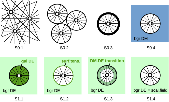
Figure 1: The considered scenarios for a connection of galactic dark matter halo with uniform background, at the top – rejected, at the bottom – accepted ones.

1 Introduction

This work continues the construction of the model [1] presented at Bled 2020 Workshop “What Comes Beyond the Standard Models?”. In this model, the sources of dark matter are Planck cores, Planck density objects located inside black holes. These objects are permanently emitting particles of dark matter, of originally Planck energy and Planck flux density. In this work, massless particles will be considered as quanta of dark matter, that are also sterile, which means that they do not enter into any interactions except gravitational. Radiation occurs in a T-symmetric way, into the future and into the past, so no energy is spent during the radiation, and such objects retain their mass. The radiation occurs in the radial direction; therefore, the considered flows have no transverse pressure. We denote this type of matter as null radial dark matter (NRDM).

The solution of Einstein’s field equations with such matter term has a structure different from the Schwarzschild’s one. This explains the designation of such compact massive objects as quasi-black holes, dark stars, Planck stars [2, 3, 4, 5]. These solutions do not have an event horizon; instead, a deep gravitational well is formed at the gravitational radius. In our model, calculations for realistic astrophysical scenarios show the redshift value $z\sim 10^{49}$, which leads to a shift of the emitted dark matter from the Planck’s $\lambda_{in}\sim 10^{-35}$m to the ultrahigh wavelengths $\lambda_{out}\sim 10^{14}$m, respectively, ultralow energies $E_{out}\sim 10^{-20}$eV. Such extreme values complicate direct detection of isolated dark matter particles. Nevertheless, the total number of emitted quanta corresponds to the initially high Planck values. The energy density and radial pressure of such radiation creates a hidden mass distribution corresponding to the observed rotation curves of galaxies. The total mass contained in such radiation, due to its extension, significantly exceeds the mass of the emitting object within its gravitational radius. The geometric mass density profile $\rho\sim r^{-2}$ typical for the radial radiation creates a linearly growing mass profile $M\sim r$ and flat rotation curves $v^{2}=GM/r=Const$. Taking into account the contributions of all black holes in the galaxy, supermassive and stellar mass ones, the distributions are modulated, and the observed nonflat rotation curves of galaxies are reproduced with good accuracy. In addition, consideration of the astrophysical scenario with the fall of an asteroid onto the Planck core leads to electromagnetic radiation with the characteristics of Fast Radio Bursts.

In this work, the main attention will be paid to the following question. If we count the massless dark matter as homogeneous (hot dark matter, HDM), then the solution of the Friedmann equations will correspond to the radiation epoch and will not coincide with the current evolution, which in the standard model corresponds to a mixture of contributions from uniform cold dark matter (CDM) and dark energy (DE). However, in the model under consideration, the distribution of matter is inhomogeneous, and, as we will see, it allows the construction of models that are in agreement with the experiment. Thus, within the framework of this model, NRDM mimics CDM at the cosmological level. The CDM macro-particles are galaxies with massive halos surrounding them.

In more detail, we will consider several scenarios for the connection of galaxies in NRDM configuration with a uniform background. The backgrounds considered are vacuum, CDM and matter with DE equation of state. In the first two cases, totally uniform DE contribution can be also added. The hydrostatic equilibrium of the system and the correspondence of the densities to the observed $\Omega$-parameters will be used as selection criteria. As a result of the analysis, it turned out that of the considered scenarios, only NRDM-DE connections meet the selection criteria. Such scenarios can be interpreted as a phase transition of dark matter from the NRDM state inside galaxies to the DE state outside. The specific mechanism for such a transition can be Bose-Einstein condensation (BEC).

In addition, we will consider the question of what happens if the dark matter particles are not exactly sterile, for example, are photons of the Standard Model.

Phase transitions between dark matter and dark energy have been addressed in a number of recent works. In [6], a phase transition in a system of two scalar fields was considered, with a massive phase of dark matter condensing around galaxies, while outside one of the fields was absent, and the other turned into an exponentially rolling mode corresponding to dark energy. Conceptually, this model expands the cosmons theory [7], in which there is only one scalar field representing dark energy in the exponentially rolling mode, while its fluctuations represent dark matter. In the works [8, 9], a phase transition similar to the Ising model of ferromagnetism was considered, effectively generating two cosmological constants during the evolution of the universe. In the works [10, 11, 12, 13] various scenarios of phase transitions at an early stage of the evolution of the universe, with the formation of bubbles of a new vacuum – dark energy were considered. In these scenarios, there was a transfer and filtration of dark matter through the walls of the bubbles, which in specific calculations reproduces its present abundance. In earlier works [14, 15], bubbles of a different vacuum after the phase transition were stabilized and led to the formation of massive compact objects – dark energy stars.

More general scenarios of the interaction of dark energy and dark matter were considered in a number of works [16, 17, 18, 19], in the framework of the so-called $Q$-phenomenology. In this approach, the components of the dark sector are considered as two massive fluids, in which, in the absence of interaction, the energies are conserved separately. When interaction is enabled between components, energy exchange occurs, parameterized by a single scalar function $Q$. For this function, one chooses linear dependencies of elementary densities, products of their degrees – by analogy with the kinetics of chemical reactions, and various other model forms. The calculation results were then compared with the cosmological observables. In works [20, 21, 22, 23, 24, 25, 26, 27, 28, 29, 30, 31, 32, 33] the interaction of dark matter and dark energy was considered in relation to cosmological tensions. These are the discrepancies between the Hubble parameter and other cosmological properties, found in different types of observations, in particular, for the early and late stages of the evolution of the universe. The direct relation of the dark matter – dark energy interaction models with cosmological tensions can be explained. In the absence of the interaction, the components of the dark sector evolve independently, being bound only by the common gravitational field. From here it is easy to obtain the individual dependences of the component densities on the scale factor of the universe. This makes directly observable variables (such as distribution of CMB inhomogeneities, luminosity-distance-redshift dependence, etc.) related with model parameters (such as Hubble parameter today, linear fluctuation of the matter density field, etc.). When the interaction is turned on, the components begin to pump into each other; as a result, the relationship of the model parameters with the observed variables is modified. A similar approach is used in the models of dynamical dark energy [34, 35, 36], where the equation of state or the density of dark energy are modified directly. The resulting changes manifest themselves as tensions between the values of the Hubble parameter, deduced from different types of measurements without model modification. Within this framework, with the right model modification, the cosmological tensions should disappear.

The idea that dark matter and/or energy are associated with Bose-Einstein condensation, are represented by a superfluid liquid, was considered in a number of works [37, 38, 39, 40, 41, 42, 43]. In particular, [43] considered a complex scalar field with a potential equivalent to Chaplygin gas. While the specific form of the potential is not important, the presence of a minimum in it is significant. In this model, the dark energy is the state of Bose-Einstein condensate, asymptotically attained by the scalar field at this minimum. Dark matter was viewed as an excited state described by a gas of quasiparticles. In our work, a similar model will be considered, in which the outer zone of the galactic halo will also be occupied by Bose-Einstein condensate, while the distribution of dark matter in the inner part of the halo will be associated with the emission of particles from RDM stars.

First, in Section 2, we will recall the structure of the RDM model, then consider a number of scenarios for its connection with a uniform background. Not all of the scenarios will be successful, but we will describe all in detail to rule out unsuccessful options. Section 3 considers separately the photon case. The details of the constructions are given in the Appendix.

2 Estimations for various scenarios

The model [1] considers three cases: massive, null or tachyon radial dark matter (M/N/T-RDM). The tachyon case is too exotic and will not be considered here. On the other hand, the massive case is similar to the commonly considered uniform cold dark matter (CDM). In this paper, we focus on the intermediate case, null or light-like dark matter. The quanta of such dark matter are massless sterile particles of an unspecified type.

The main formulas that determine the distribution of masses and pressures of dark matter in the model under consideration are

$$\rho=p_{r}=\epsilon/(8\pi r^{2}),\ p_{t}=0,\ \rho_{grav}=\rho+p_{r}+2p_{t},$$ (1)

where $\rho$ is the mass density, $p_{r}$ is the radial pressure, $p_{t}$ is the transverse pressure, $\rho_{grav}$ is the gravitating mass density, $r$ is the radius, $\epsilon$ is constant scaling parameter, in the geometric system of units $G=c=1$. Such dependence’s are established at large distances from the center of the galaxy, when all sources of dark matter (RDM stars), distributed over the galaxy in proportion to the density of the luminous matter, can be considered as concentrated in one center. The integrated gravitating mass for such a distribution is linear in the radius: $M_{grav}=\epsilon r$, and the square of the orbital velocity is constant and equal to $v^{2}=M_{grav}/r=\epsilon$.

In relation to the $\epsilon$-parameter for the Milky Way (MW) galaxy, [1] provides several estimates. The simplest, if one places a single RDM star in the center of the galaxy and completely neglect the contribution of the luminous matter, leads to a flat rotation curve with an orbital velocity $v\sim 200$km/s, $\epsilon=(v/c)^{2}\sim 4\cdot 10^{-7}$. A more accurate estimate is obtained from the fit of the MW rotation curve, the so-called Grand Rotation Curve (GRC, [44, 45, 46, 47, 48]). From this fit it can be seen, [1] Fig.2, that on an approximately flat portion of the rotation curve at the position of the Sun $r\sim 8$kpc there is a significant contribution of luminous matter, as a result of which the contribution of dark matter to $v^{2}$ is less than the trivial estimate. Further, with increasing radius, the contribution of luminous matter decreases, while the contribution of dark matter remains constant up to $R_{cut}\sim 50$kpc. This contribution corresponds to the galactic $\epsilon=M_{dm}(R_{cut})/R_{cut}$, in geometric units, being averaged over the scenarios considered in [1]: $M_{dm}(R_{cut})\sim 2.6\cdot 10^{11}M_{\odot}$, $\epsilon\sim 2.5\cdot 10^{-7}$. In this work, we will carry out estimates in order of magnitude, so it is not so important which definition of the galactic $\epsilon$ will be chosen. We prefer the latter, more precise definition and the corresponding value $M_{dm}(R_{cut})$.

When the contribution of individual black holes (identified with RDM stars) is considered, [1] Fig.5 gives estimates for the central supermassive and peripheral stellar black holes: $\epsilon_{smbh}\sim 10^{-10}-10^{-7}$, $r_{s,smbh}\sim 1.2\cdot 10^{10}$m; $\epsilon_{sbh}\sim 10^{-16}-10^{-12}$, $r_{s,sbh}\sim 3\cdot 10^{4}$m. This gives a floating estimate for the external wavelength of DM particles: $\lambda_{out}=r_{s}(8\pi/\epsilon)^{1/2}$, $\lambda_{out,smbh}\sim 10^{14}-10^{16}$m, $\lambda_{out,sbh}\sim 10^{11}-10^{13}$m. This wavelength is highly dependent on the model used to describe the internal structure of RDM stars. In this work, for estimations, we prefer to use the value of the external wavelength $\lambda_{out}$ and the corresponding redshift factor $A_{QG}^{1/2}=l_{P}/\lambda_{out}$ as phenomenological parameters.

The considered scenarios for the connection of galaxies in the NRDM configuration with a uniform background are schematically shown in Fig.1.

2.1 Rejected scenarios

Scenario S0.1: superposition of galactic halos without cutting.

In this scenario, the dark matter halo of each galaxy extends to the radius of the visible universe $R_{uni}\sim 14$Gpc, dark matter from different halos does not interact and gives an additive contribution to the total mass density. If this scenario was valid, then it would be different from the radiation epoch, due to the following reasons. For the radiation epoch, the Big Bang (more precisely, the moment of recombination) is the initial flash, after which the homogeneous photon gas cools down as the universe expands. The energy of the photons changes with the scale factor as $a^{-1}$, and their numerical density as $a^{-3}$, which gives the dependence $a^{-4}$ for the mass density. For the RDM model, despite the expansion of the universe and the separation of RDM stars from each other, the energy of DM particles near RDM stars is fixed, related to the above-mentioned parameter $\lambda_{out}$. It is important that this energy does not fall over time. The number density of RDM stars falls as $a^{-3}$, and as a result the average mass density also falls as $a^{-3}$, just like for CDM.

The scenario is prohibited due to the following evaluation. According to calculations for the Milky Way galaxy [1], the cutoff radius and halo mass are $R_{cut}\sim 50$kpc, $M_{dm}(R_{cut})\sim 2.6\cdot 10^{11}M_{\odot}$, and the mass of the disk and other emitting structures can be neglected in the order estimate. If one does not use the cutoff and continues the halo to the border of the universe, $M_{dm}(R_{uni})=M_{dm}(R_{cut})R_{uni}/R_{cut}\sim 7.3\cdot 10^{16}M_{\odot}$. If the result is multiplied by the estimated number of galaxies in the universe $N_{gal}\sim 2\cdot 10^{12}$, we get $M_{dm}\sim 1.5\cdot 10^{29}M_{\odot}$. Compared to the estimated mass of dark matter in the universe $M_{dm,uni}\sim 4.5\cdot 10^{23}M_{\odot}$, this value is overestimated by the factor $\sim 3.2\cdot 10^{5}$. The mass density averaged over the volume of the universe for the obtained value of $M_{dm}$ will be $\rho_{dm}\sim 8.6\cdot 10^{-22}kg/m^{3}$, which in $\sim 3.2\cdot 10^{5}$ more than the estimate from the critical density $\Omega_{dm}\rho_{crit}=2.7\cdot 10^{-27}kg/m^{3}$.

The following corrections can be made to this calculation. The geometric cutoff by $R_{uni}$ for the galaxies located far from the center (which we locate in the MW) can reduce the halo mass, but the factor is small, at most $2$. The mass density is everywhere understood as the gravitating mass density, which also includes the pressure $\rho_{grav}=\rho+p_{r}$. At cosmological distances, the energy of DM particles is redshifted, but considering distances up to $0.03R_{uni}\sim 420$Mpc, the mass density decrease factor will not exceed 20% (for the Hubble parameter $H_{0}=72$km/s/Mpc such distances correspond to $z\sim 0.1$, 10% decrease in energy and 10% slowdown in time, affecting 20% decrease in flux density). This can be used to estimate the mass from below, as a result the $>7.6\cdot 10^{3}$ discrepancy will remain unexplained.

Further, the estimate is based on the assumption that all galaxies have masses of the order of the MW. This, of course, is not the case, there is a distribution of galaxies by masses. An accurate account of the distribution of galaxies will be given in the Appendix, and a similar result will be obtained, within the accuracy of modeling the distribution of galaxies.

Now we assume that all galaxies are copies of the MW, the halo of each galaxy is extended to the radius $R_{gal}$ and the relation $N_{gal}M_{dm}(R_{cut})/R_{cut}\cdot R_{gal}=M_{dm,uni}$ holds, at which all the necessary mass relations are joined. Substituting the known data, we get $R_{gal}=44$kpc, which almost coincides with the value of $R_{cut,MW}$. An exact match of $R_{gal}=R_{cut,MW}$ can be achieved by slightly adjusting the estimated number of galaxies to $N^{\prime}_{gal}=1.7\cdot 10^{12}$. Thus, according to this estimate, if we imagine that the universe consists of copies of the MW galaxy, the halo of which is cut off by $R_{cut}\sim 50$kpc, then the total mass of dark matter in the universe will coincide in order of magnitude with its cosmological estimate. With this configuration, dark matter is entirely concentrated in galaxies and is absent in the intergalactic environment.

Let’s find out what happens if the $R_{cut}$ parameter is increased to 1Mpc. This is possible when the estimated number of galaxies is reduced to $N^{\prime}_{gal}\sim 8.7\cdot 10^{10}$. It is known that the mass-to-light ratio of galaxies stops changing at distances of this order of magnitude, see [49] Fig.2.5. Moreover, this value is of the order of intergalactic distances. Thus, a scenario is theoretically possible in which galaxies touch each other in the outer zones of their halos, although it may require tensions of the $N_{gal}$ parameter.

Finally, for the original scenario in which the halos overlap and reach the size of the universe, it would be $N^{\prime}_{gal}\sim 6.2\cdot 10^{6}$, a too strong deviation from the observed value. Therefore, this scenario can be considered as excluded.

Scenario S0.2: touching halos in dynamic equilibrium.

The above variant with halos touching each other in the outer region, with the refinement that galaxies can exchange dark matter. Null dark matter leaking from one galaxy is absorbed by neighboring galaxies, and vice versa. In fact, the world lines of dark matter form a network connecting the galaxies, and the concept of a spherical halo is only an approximation.

The problem here is as follows. As a result of the expansion of galaxies, DM particles coming from neighboring galaxies are subject to a small redshift $z$ and decrease their energy and flux density by the corresponding factor. We consider RDM stars in a stationary T-symmetric scenario. The parameters of dark matter, in particular, its energy and flux density, coincide for the incoming and outgoing flows. Therefore, the exiting particles also have a reduced energy and flux density. With multiple reflections between galaxies, the redshift of DM particles accumulates, exactly as it would in a homogeneous environment. RDM stars act as spherical mirrors, changing the direction of the DM particles, but not their energy characteristics. Such an environment turns out to be equivalent to HDM, its evolution coincides with the era of radiation, which is different from the observed evolution of the universe today.

In fact, the stationary state of RDM stars requires T-symmetry only for the energy flux density $\epsilon$, the individual energies of incoming and outgoing DM particles can be different, compensated by different number flux densities. This will not help, since it is energy density that governs cosmological evolution. Note also that in the equation $\rho_{P}=\epsilon/(8\pi r_{s}^{2}A_{QG})$, which determines conditions on the surface of the Planck core, in the considered scenario the factors $\epsilon$ and $A_{QG}$ are scaled equally so that the gravitational radius $r_{s}$ can remain unchanged. Strictly speaking, changing $\epsilon$ and $A_{QG}$ in stationary scenarios is also unacceptable, but we consider this change as performed rather slowly, quasi-statically. What happens in fast scenarios, as well as with T-asymmetric $\epsilon$ and variable $r_{s}$, can be found out only after solving the dynamic RDM problem, which goes beyond the scope of this work.

Scenario S0.3: a halo surrounded by a massive thin shell.

We now look at a few scenarios from the termination shock type. This phenomenon occurs at the edge of the solar system when the radially directed solar wind meets the isotropic interstellar medium. Similar phenomena can occur with dark matter at the edge of the galaxy when the radial flow of dark matter meets the intergalactic environment. First, we will consider a scenario in which an NRDM galaxy at radius $R_{cut}$ is surrounded by a thin CDM layer, and there is a vacuum outside. The CDM layer is held in equilibrium by the NRDM pressure force and the force of gravity. If such a scenario was possible, the galaxies would be isolated from each other and would be massive balls floating in a vacuum. On a cosmological level, such matter is equivalent to CDM.

The equilibrium condition of forces can be written as $\epsilon/(8\pi r^{2})\cdot 4\pi r^{2}=\epsilon/r\cdot m$ for $r=R_{cut}$, whence the mass of the CDM layer $m=R_{cut}/2$, in geometric units. This is a huge mass, exceeding the mass of the galaxy $M_{dm}(R_{cut})=\epsilon R_{cut}$, where $\epsilon\ll 1$, for MW $\epsilon=2.5\cdot 10^{-7}$. Formally, with such a mass, the galaxy is covered by its event horizon, becoming a black hole. More precisely, the calculation uses Newtonian equations and only shows that there is no solution in weak fields. The interpretation of this result is that the relativistic pressure at the boundary of the NRDM galaxy can be compensated only by relativistic gravitational forces.

The distribution of matter in the CDM layer obeys the Tolman-Oppenheimer-Volkoff (TOV) equation, the solution of which in weak fields and for a thin layer is described by the one-dimensional hydrostatic equation $\rho=\rho_{0}\exp(-gh/w)$, where $w$ - parameter of the equation of state (EOS) $p=w\rho$, for CDM $w=kT/m\ll 1$, all equations are written in geometric units. The pressure equilibrium at the boundary of the layer leads to $\epsilon/(8\pi R_{cut}^{2})=w\rho_{0}$, also $g=\epsilon/R_{cut}$, whence $\rho=\epsilon/(8\pi R_{cut}^{2}w)\cdot\exp(-\epsilon h/(wR_{cut}))$. Integrating this value, we get $m=4\pi R_{cut}^{2}\int\rho dh=R_{cut}/2$. The result is independent of $w$ and coincides with the estimate above.

Scenario S0.4: halo surrounded by homogeneous dark matter.

A variation of the previous scenario, where instead of vacuum there is a homogeneous dark matter with isotropic EOS outside: $p_{bgr}=w\rho_{bgr}$. Here we will consider two options: CDM $w\ll 1$, HDM $w=1/3$. Pressure equilibrium at the halo boundary: $\epsilon/(8\pi R_{cut}^{2})=w\rho_{bgr}$, gravitating masses: $M_{dm,gal}=N_{gal}\epsilon R_{cut}$, $M_{dm,bgr}=(1+3w)\rho_{bgr}\cdot(4\pi/3)(R_{uni}^{3}-N_{gal}R_{cut}^{3})$, an estimate of the total mass of dark matter in the universe: $M_{dm,uni}=M_{dm,gal}+M_{dm,bgr}=N_{gal}\epsilon R_{cut}+\epsilon(1+3w)/(6wR_{cut}^{2})(R_{uni}^{3}-N_{gal}R_{cut}^{3})$. Note that, according to earlier calculations, the first term already corresponds in order to the cosmological estimate for the mass of dark matter. Only if the second term is small, this correspondence could be preserved. However, if we assume that the intergalactic distances significantly exceed the size of the halo, and the estimate $R_{uni}^{3}\gg N_{gal}R_{cut}^{3}$ holds, then the second term $M_{dm,uni}\sim\epsilon R_{uni}^{3}/R_{cut}^{2}\cdot(1+3w)/(6w)$, which for $\epsilon=2.5\cdot 10^{-7}$, $R_{uni}\sim 14$Gpc and $R_{cut}\sim 50$kpc matches $M_{dm,uni}/M_{\odot}\sim 5.7\cdot 10^{27}(1+3w)/(6w)$. It can be seen that already for $w=1/3$ and even more so for $w\ll 1$ the result significantly exceeds the value $M_{dm,uni}/M_{\odot}\sim 4.5\cdot 10^{23}$, obtained from cosmological estimates. Also for the above option with tension, $R_{cut}=1$Mpc, $N^{\prime}_{gal}=8.7\cdot 10^{10}$ the resulting formula is $M_{dm,uni}/M_{\odot}=4.5\cdot 10^{23}+1.4\cdot 10^{25}(1+3w)/(6w)$ does not allow CDM/HDM as background matter, for continuous matching with NRDM pressure at halo boundaries.

2.2 Accepted scenarios

Next, we’ll look at scenarios involving dark energy. We will represent dark energy as a kind of matter, perhaps a kind of dark matter or its other phase state, which has an isotropic EOS $p_{de}=-\rho_{de}$, that is, $w=-1$, with positive $\rho_{de}$, constant within each phase. The density of the gravitating mass for such matter is negative and is equal to $\rho_{de,grav}=\rho_{de}+3p_{de}=-2\rho_{de}$. The negativity of this density, provided that it prevails over other components, is the driving mechanism for the accelerated expansion of the universe.

Scenario S1.1: jump in the dark energy density at the halo boundary.

Let there be two different dark energy densities, outside the halo $\rho_{de,bgr}$, inside the halo $\rho_{de,gal}$, with a jump at $R_{cut}$. Equilibrium pressure condition $\epsilon/(8\pi R_{cut}^{2})=p_{de,bgr}-p_{de,gal}=\rho_{de,gal}-\rho_{de,bgr}$, gravitating masses: $M_{dm,gal}=N_{gal}\epsilon R_{cut}$, $M_{de,gal}=-2\rho_{de,gal}N_{gal}\cdot(4\pi/3)R_{cut}^{3}$, $M_{de,bgr}=-2\rho_{de,bgr}\cdot(4\pi/3)(R_{uni}^{3}-N_{gal}R_{cut}^{3})$, an estimate of the total mass of dark matter and dark energy in the universe: $M_{dm+de,uni}=M_{dm,gal}+M_{de,gal}+M_{de,bgr}=(2/3)\epsilon N_{gal}R_{cut}-(8\pi/3)\rho_{de,bgr}R_{uni}^{3}$. The second term here describes the total gravitating mass of dark energy, as if it uniformly filled the entire universe, including galactic halos. The first term is the gravitating mass of the galactic halo reduced by the factor $(2/3)$. In general, the model behaves like a mixture of uniform cold dark matter and uniform dark energy, like $\Lambda$CDM. In order of magnitude, for $R_{cut}=50$kpc, the CDM mass corresponds to cosmological estimates. Fine tuning is also possible similar to scenario S0.1, the factor $(2/3)$ can be compensated for by a small increase in the estimated number of galaxies $N^{\prime}_{gal}=2.6\cdot 10^{12}$.

Let us also analyze the expression for the gravitating mass of one galaxy: $M(r)=\epsilon r-2\rho_{de,gal}(4\pi/3)r^{3}$. In the expression for the internal dark energy density $\rho_{de,gal}=\epsilon/(8\pi R_{cut}^{2})+\rho_{de,bgr}$ for the selected value $R_{cut}=50$kpc, after conversion to natural units, the first term is $5.6\cdot 10^{-24}kg/m^{3}$, the second $\rho_{de,bgr}=\Omega_{de}\rho_{crit}=6.8\cdot 10^{-27}kg/m^{3}$, the first term dominates. Thus, continuous matching of pressures at the galactic boundary requires a jump in the dark energy density by a factor of $\sim 10^{3}$. Note that this jump can be reduced by adjusting the $R_{cut}$ parameter.

Further, the expression for the mass function at the selected parameters becomes $M(r)/M_{\odot}=2.6\cdot 10^{11}(r/R_{cut})-8.7\cdot 10^{10}(r/R_{cut})^{3}$. In the inner part of the rotation curve, for example, up to the position of the Sun $r\sim 8$kpc, the first term dominates. Thus, the interior of the rotation curve is unaffected by the dark energy introduced into the model. In the outer part of the curve, the contribution of the enhanced internal dark energy density becomes noticeable, finally, it is this contribution that leads to the factor $(2/3)$ in the mass formulas. The term proportional to the external dark energy density for the chosen parameters of the model makes a negligible contribution within the galaxy. It begins to dominate in the formula $M(r>R_{cut})=(2/3)\epsilon R_{cut}-(8\pi/3)\rho_{de,bgr}r^{3}$ at distances $r>0.6$Mpc, at which the effects of cosmological expansion become noticeable.

It becomes clear that in the considered scenario the rotation curve undergoes a change only in its outer part, where it decreases by $\sqrt{2/3}$ factor, about $18\%$. As we will see later, the measurement errors in this range significantly exceed this variation, which makes it impossible to distinguish this solution from the reference profile.

Thus, we have obtained the first scenario, which connects null matter in galactic halos with a cosmological background of dark energy and turns out to be equivalent to the uniform $\Lambda$CDM model. A calculation based on a simple equilibrium of pressures does not provide any indication for the possible nature of the increased density of dark energy within the galaxy. Phenomenologically, dark energy can be described as a medium in which its constituent particles experience mutual attraction. This attraction corresponds to negative pressure, while the work of external forces $-pdV$ is used to increase the internal energy $\rho dV$, in accordance with EOS $-p=\rho$. The presence of two phases with different pressures suggests two varieties for such media. An analogy can be drawn here with the string model. The energy of a string is proportional to its length, just like the total mass for dark energy is proportional to its volume. The strings have a fixed tension, which is a constant in the model. One can consider strings with different tensions as separate varieties of the same model. The considered scenario demonstrates a fundamental possibility; further possible alternatives will be considered.

Scenario S1.2: surface tension at the boundary between the halo and the background from dark energy.

Let inside $R_{cut}$ be NRDM, outside – dark energy with density $\rho_{de,bgr}$, and surface tension with coefficient $\sigma$ acts on the boundary. Equilibrium pressure condition $\epsilon/(8\pi R_{cut}^{2})=2\sigma/R_{cut}+p_{de,bgr}=2\sigma/R_{cut}-\rho_{de,bgr}$, gravitating masses: $M_{dm,gal}=N_{gal}\epsilon R_{cut}$, $M_{de,surf}=-N_{gal}\sigma\cdot 4\pi R_{cut}^{2}$, $M_{de,bgr}=-2\rho_{de,bgr}\cdot(4\pi/3)(R_{uni}^{3}-N_{gal}R_{cut}^{3})$, an estimate of the total mass of dark matter and dark energy in the universe: $M_{dm+de,uni}=M_{dm,gal}+M_{de,surf}+M_{de,bgr}=(3/4)\epsilon N_{gal}R_{cut}+(2\pi/3)\cdot N_{gal}R_{cut}^{3}\rho_{de,bgr}-(8\pi/3)\rho_{de,bgr}R_{uni}^{3}$. Here the third term corresponds to the cosmological contribution of dark energy, it grows in the negative direction in proportion to the volume of the expanding universe. The first and second terms are preserved in the expansion and represent CDM. At $R_{cut}=50$kpc, the first term significantly exceeds the second, and, as in the previous scenario, allows fine tuning of the parameters to the cosmological value of CDM density.

In the above formulas, the gravitating mass corresponding to the boundary layer is calculated as follows. Surface tension is related to negative transverse pressure and positive energy density as $-p_{t}=\rho=\sigma/dr$, where $dr$ is the layer thickness. The gravitating mass of the spherical layer is $M=(\rho+2p_{t})Sdr=-\sigma\cdot 4\pi R_{cut}^{2}$. There is also a radial pressure $p_{r}$ inside the layer, which continuously interpolates the boundary values, remains bounded, and makes a vanishing contribution at $dr\to 0$.

When choosing $R_{cut}=50$kpc, the density jump between external dark matter and NRDM is still $\sim 10^{3}$ times, but here it is compensated by surface tension. As in the previous scenario, the pressure jump can be reduced by adjusting the $R_{cut}$ parameter. The mass function for $r<R_{cut}$ coincides with the NRDM dependence $M(r<R_{cut})=\epsilon r$, thus the inner rotation curve does not change. When passing through $R_{cut}$, the mass function undergoes a jump $M(R_{cut}+0)=(3/4)\epsilon R_{cut}-2\pi R_{cut}^{3}\rho_{de,bgr}$, the coefficient $(3/4)$ appears in the first term, and the second term also appears. With the chosen parameters, the first term is $1.9\cdot 10^{11}M_{\odot}$, the second $-7.9\cdot 10^{7}M_{\odot}$, the first term dominates. Further, the mass function includes the cosmological term $M(r>R_{cut})=(3/4)\epsilon R_{cut}+(2\pi/3)R_{cut}^{3}\rho_{de,bgr}-(8\pi/3)\rho_{de,bgr}r^{3}$, which dominates for $r>0.6$Mpc.

The resulting scenario is very close to the previous one, only a different mechanism is used to compensate for the pressure jump at the edge of the galaxy. Phenomenologically, if we consider dark energy as a medium consisting of interacting particles, the presence of a boundary can lead to the appearance of a surface term in the equations, as for classical media. The jump in the mass function that appears in this scenario corresponds to a jump in the rotation curve by the factor $\sqrt{3/4}$, about 13%. This jump also occurs in the outer region, where the scatter of experimental data is large, so that it can be unnoticed. Also, this jump can be an idealization of a more complex scenario in which the transition layer has a finite thickness. The possibility of a gradual change of EOS will be explored in the following scenario.

Scenario S1.3: phase transition of dark matter to dark energy.

In this scenario, we assume that dark energy is a form of dark matter, and with the increasing radius, there is a continuous transition between the corresponding EOS: $p_{r}=w_{r}\rho$, $p_{t}=w_{t}\rho$, $(w_{r},w_{t})$ change from $(1,0)$ for $r=R_{cut1}$ to $(-1,-1)$ for $r=R_{cut2}>R_{cut1}$. The result depends on the transition path, which we fix from physical considerations as follows. Initially, from $r=R_{cut1}$ to the intermediate point $r=R_{cut1b}$, only $w_{t}$ changes, from $0$ to $-1$. The inclusion of transverse attraction between flows of dark matter leads to the Joule-Thomson effect known in gas dynamics, cooling of flows, which in our case manifests itself in a rapid decrease in the mass density $\rho$. Further, from $r=R_{cut1b}$ to $r=R_{cut2}$ only $w_{r}$ changes, from $1$ to $-1$. In this range, the contributions of dark matter from different sources are mixed, the matter becomes isotropic. Further, the matter obeys isotropic EOS for dark energy, and its density and pressure become constant.

It is convenient to solve the problem in logarithmic variables $x=\log r$, $\xi=\log\rho$, with the restriction $\rho>0$. To interpolate $w_{t,r}$ in the corresponding intervals, we choose functions linear in $x$, and the positions of the endpoints $\{x_{1},x_{1b},x_{2}\}=\log\{R_{cut1},R_{cut1b},R_{cut2}\}$ will be chosen from the correspondence of the model to the cosmological parameters.

The stationary spherically symmetric solutions considered here satisfy the hydrostatic equation for anisotropic medium, see Appendix for details: $r(p_{r}+\rho)A^{\prime}_{r}+2A(r(p_{r})^{\prime}_{r}+2p_{r}-2p_{t})=0$. The first term describes the gravitational interaction, which in our problems can be neglected. The reason for this is that in the weak field limit $A\sim 1+2\phi$, $A^{\prime}_{r}\sim 2g$, where $\phi$ is the gravitational potential, $g=\phi^{\prime}_{r}=M_{grav}(r)/r^{2}$ is gravitational field in the used system of units, $|\phi|\ll 1$, $rg\ll 1$. In our models, the density and pressure are controlled by a small common factor $\epsilon$, and the first term turns out to be of the next smallness order compared to the second one. This property of the weak-field regime can also be verified on the exact solutions of the hydrostatic equation, given in Appendix.

Thus, we can concentrate on the second term: $r(p_{r})^{\prime}_{r}+2p_{r}-2p_{t}=0$. Let’s go to logarithmic variables and substitute EOS: $w_{r}\xi^{\prime}_{x}+(w_{r})^{\prime}_{x}+2(w_{r}-w_{t})=0$. The solution is: $\xi=-\int dx((w_{r})^{\prime}_{x}+2(w_{r}-w_{t}))/w_{r}$. In the following, we will consider regular solutions in which the denominator and the numerator in the integrand vanish simultaneously: $w_{r}=0$, $(w_{r})^{\prime}_{x}=2w_{t}$. Note that, with our choice of the interpolation order, the condition $w_{r}=0$ can be satisfied only at the second stage, in the interval $[x_{1b},x_{2}]$, while, due to the linearity of the interpolation, the condition $(w_{r})^{\prime}_{x}=2w_{t}=-2$ holds on this entire interval.

At the first stage $[x_{1},x_{1b}]$, $(w_{r},w_{t})=(1,-q)$, $q=(x-x_{1})/(x_{1b}-x_{1})$, calculating the integral, we get $\xi_{1b}-\xi_{1}=-3(x_{1b}-x_{1})$. At the second stage $[x_{1b},x_{2}]$, $(w_{r},w_{t})=(1-2q,-1)$, $q=(x-x_{1b})/(x_{2}-x_{1b})$, from the condition $(w_{r})^{\prime}_{x}=-2$ we get $q^{\prime}_{x}=1$, that is, $x_{2}=x_{1b}+1$. Calculating the integral, we get $\xi_{2}-\xi_{1b}=-2$. Hence $\log(\rho_{1}/\rho_{2})=\xi_{1}-\xi_{2}=3(x_{1b}-x_{1})+2$. Choosing $\rho_{1}=\epsilon/(8\pi R_{cut1}^{2})$, $R_{cut1}=R_{cut}=50$kpc, $\epsilon=2.5\cdot 10^{-7}$, $\rho_{2}=\rho_{de,bgr}=\Omega_{de}\rho_{crit}=6.8\cdot 10^{-27}kg/m^{3}$, and also converting all values into the natural system of units, we get: $\rho_{1}/\rho_{2}=824$, $R_{cut1b}=0.24$Mpc, $R_{cut2}=0.65$Mpc. Thus, the required density variation from NRDM to the background dark energy in the considered scenario fixes the halo cutoff parameters to reasonable values.

Next, consider the contribution of the galaxy to the cosmological mass density. The gravitating mass density is $\rho_{grav}=(1+w_{r}+2w_{t})\rho$, and the gravitating mass of the spherical layer is $\Delta M_{grav}=4\pi\int\rho_{grav}r^{2}dr$. After the transition to logarithmic variables, the integrals over two interpolation intervals can be taken analytically. Omitting cumbersome expressions, we will immediately give the numerical answer $\{M_{1},\Delta M_{1},\Delta M_{2},M_{vac}\}=\{2.60,2.67,-2.60,2.35\}\cdot 10^{11}M_{\odot}$. Here $M_{1}=\epsilon R_{cut}$ is the mass of the NRDM halo, $\Delta M_{1,2}$ are the masses of the spherical layers for two interpolation intervals, $M_{vac}=(8\pi/3)\rho_{de,bgr}R_{cut2}^{3}$ is the compensation mass of the vacuole arising from the rearrangement of the terms $M_{dm+de,uni}=N_{gal}M_{dm+de,gal}-(8\pi/3)\rho_{de,bgr}(R_{uni}^{3}-N_{gal}R_{cut2}^{3})=N_{gal}(M_{dm+de,gal}+M_{vac})-(8\pi/3)\rho_{de,bgr}R_{uni}^{3}$. The $M_{vac}$ term should be taken into account in cosmological calculations, when reducing to the parameters of a homogeneous medium, while when calculating the rotation curves only the actually present masses should be taken, and $M_{vac}$ should be omitted. Interestingly, there is an identity $M_{1}+\Delta M_{2}=0$, which holds exactly, at the analytical level, but is probably a coincidence due to a special choice of interpolating functions. Also of interest is the approximate equality of all mass contributions in their absolute value. The cosmological mass per galaxy is the sum of all these contributions and is equal to $M_{dm+de,gal}+M_{vac}=5\cdot 10^{11}M_{\odot}$. This gives a coincidence with the cosmological CDM mass $M_{dm,uni}=4.5\cdot 10^{23}M_{\odot}$ in order of magnitude, for exact coincidence the estimated number of galaxies should be reduced to $N^{\prime}_{gal}=9\cdot 10^{11}$, 2.2 times less than the nominal value. One can also adjust the $\epsilon$ parameter, but since our estimates of the halo cutoff parameters were tied to MW values, these estimates must be repeated when $\epsilon$ changes.

The constructed scenario, obviously, contains wide arbitrariness in the choice of interpolating functions and is rather a proof of the existence of a solution satisfying cosmological estimates. This existence in itself is non-trivial. Recall that in standard cosmology, null, hot dark matter leads to a different rate of cosmological expansion today and is forbidden. The possibility of joining hot dark matter with dark energy within the galactic halo, at a cosmological level equivalent to $\Lambda$CDM, is the main result of this work. The specific way of joining may be different, in the Appendix we will discuss the possibility of narrowing this arbitrariness.

For now, note that the interpolation order selected in the model is significant. The reverse order when $(w_{r},w_{t})$ changes from $(1,0)$ to $(-1,0)$ for $r\in[R_{cut1},R_{cut1b}]$ leads to the condition $(w_{r})^{\prime}_{x}=2w_{t}=0$, not feasible for linear functions. If we interpolate both terms at the same time, $(w_{r},w_{t})=(1-2q,-q)$, $q=(x-x_{1})/(x_{2b}-x_{1})$, from the conditions $w_{r}=0$ , $(w_{r})^{\prime}_{x}=2w_{t}$ we get $q=1/2$, $q^{\prime}_{x}=1/2$, that is, $x_{2b}=x_{1}+2$. Moreover, $\xi_{2b}=\xi_{1}-2$, which for $R_{cut1}=50$kpc gives $R_{cut2b}=e^{2}R_{cut1}=0.37$Mpc, $\rho_{1}/\rho_{2b}=e^{2}\sim 7.4$, far from the experimental value of $\rho_{1}/\rho_{2}\sim 824$. The physical rationale with the initial cooling of dark matter due to the Joule-Thomson effect and the subsequent transition to the isotropic phase for the cooled gas was important for obtaining the strong density drop observed in real galaxies.

Here are some graphs showing the behavior of the main physical profiles in the considered scenario. Fig.2 left shows the dependence of $\xi=\log\rho$ on $x=\log r$. Initially, the graph contains an NRDM line with a slope of $-2$, which corresponds to the $\rho\sim r^{-2}$ dependence. Further, at point 1, the transverse interaction between the flows turns on, and the Joule-Thomson effect is superimposed on the continuing radial drop in density. Here, the slope of the graph $d\xi/dx$ is continuously changing from $-2$ to $-4$. Further, in the interval from 1b to 2, a transition to the isotropic phase follows, the slope in this case being equal to $-2$. After point 2, there is isotropic dark energy with constant density, slope $0$. The resulting density variation between points 1 and 2 corresponds to the experimentally observed factor of $\rho_{1}/\rho_{2}\sim 824$.

For comparison, the option shown in gray when $(w_{r},w_{t})$ are linearly interpolated at the same time. The slope between points 1 and 2b is $-1$. After 2b, there is an isotropic phase with a slope of $0$. Due to these changes, the graph goes much higher than the previous one, the density variation does not correspond to the observed value.

Fig.2 right shows the dependence of $M_{grav}(r)$. Initially, there is an NRDM part with a characteristic linear dependence, then at point 1b, the dependence passes through a maximum and, after point 2, is described by a negative cubic term corresponding to the contribution of dark energy.

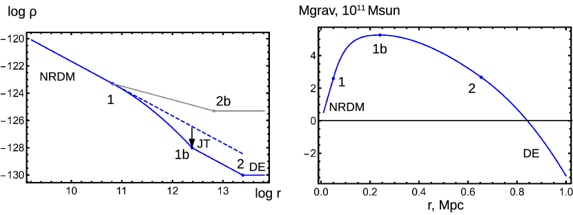
Figure 2: Physical profiles for scenario S1.3.

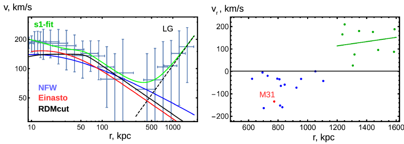
Figure 3: Left: an external part of the Milky Way rotation curve, according to [48]. A variety of profiles are shown, including the RDMcut scenario from [1]. Right: outer part of the dependence of radial velocity on the distance, according to [46]. The position of the galaxy M31 is marked, the outer part of the graph is fitted with a Hubble-alike dependence.

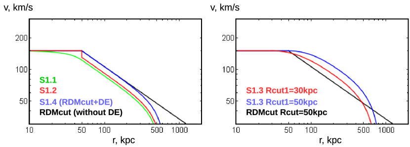
Figure 4: Profiles built in the scenarios of this work, compared with the RDMcut profile.

Scenario S1.4: Bose-Einstein condensation.

In this scenario, two phases are also considered: the internal NRDM phase, described by the classical particle model, and the external phase, described by a complex scalar field. This field theory is used in phenomenological models of Bose-Einstein condensation, as well as in cosmological models of quintessence and its variants (k-essence, quartessence, Chaplygin gas), see [43] and references therein. Therefore, this scenario assumes that dark matter particles are emitted by RDM stars in the galaxy and undergo Bose-Einstein condensation at large distances. Alternatively, these can be particles of different types that are in contact equilibrium at the edge of the galactic halo.

In the field theory under consideration, the Lagrangian, the energy-momentum tensor, and the equations of motion have the form [50] Chap.6.3,7.5:

$$L=-(\partial_{\mu}\phi^{*}\partial^{\mu}\phi)/2-V(|\phi|^{2}),$$ (2)

$$T_{\mu\nu}=(\partial_{\mu}\phi^{*}\partial_{\nu}\phi+\partial_{\nu}\phi^{*}\partial_{\mu}\phi)/2+g_{\mu\nu}L,$$ (3)

$$(-\partial^{2}/\partial t^{2}+\Delta)\phi=2V^{\prime}(|\phi|^{2})\phi.$$ (4)

Here the equations of motion are written in a flat background, and the rest of the expressions are valid for an arbitrary metric. We also remind that for a scalar field the covariant and coordinate derivatives are equal: $\nabla_{\mu}\phi=\partial_{\mu}\phi$. The field equations belong to the well-known nonlinear Klein-Gordon type with the potential. For $V(|\phi|^{2})=Const+m^{2}|\phi|^{2}/2$ the equations become linear and describe the behavior of a free massive scalar field. We neglect the influence of gravity on the scalar field, assuming that the gravitational fields are weak and the corresponding solutions are relativistic.

We will use a smooth potential $V(s^{2})$, which has a minimum for a nonzero value of the argument $V(s_{1}^{2})=V_{min}$, $s_{1}^{2}>0$. For this minimum, the constant function $\phi=s_{1}$ is the exact solution to the problem. For such a function, using a spherical coordinate system and a metric of signature $(-+++)$, we write out the mixed components of the energy-momentum tensor:

$$T_{\mu}^{\nu}=\mathop{\mbox{diag}}(-\rho,p_{r},p_{t},p_{t})=-V_{min}\cdot\mathop{\mbox{diag}}(1,1,1,1),$$ (5)

$$\rho=V_{min},\ p_{r}=p_{t}=-V_{min},$$ (6)

$$\rho_{grav}=\rho+p_{r}+2p_{t}=-2V_{min}.$$ (7)

The result coincides with the standard EOS of dark energy, which explains the interest to this model in the cosmological context. We will fix $V_{min}>0$, and for simplicity we will assume $V>0$ everywhere.

In this paper, we consider stationary spherically symmetric problems for which there are particular solutions of the form $\phi=e^{iEt}s(r)$, with real $E,s(r)$. With this substitution, the dimension is reduced $(E^{2}+\Delta)s=2V^{\prime}(s^{2})s$. Next, we will consider stationary solutions $E=0$, $\phi=s(r)$. The uniqueness of solutions with stationary boundary conditions is demonstrated in the Appendix. Thus, all solutions that can be attached to the constant $\phi=s_{1}$ are globally stationary and have the form $\phi=s(r)$.

Calculating EOS for stationary solutions

$$T_{\mu}^{\nu}=\mathop{\mbox{diag}}(0,s^{\prime 2},0,0)-\mathop{\mbox{diag}}(1,1,1,1)\cdot(s^{\prime 2}/2+V(s^{2})),$$ (8)

$$\rho=-p_{t}=s^{\prime 2}/2+V(s^{2})>0,\ p_{r}=s^{\prime 2}/2-V(s^{2}),$$ (9)

$$\rho_{grav}=\rho+p_{r}+2p_{t}=-2V(s^{2}).$$ (10)

If the potential is shallow, then $\rho_{grav}\sim-2V_{min}$, as for DE. This result is quite remarkable. As a consequence, the scenario can be configured in such a way that the gravitating density profile immediately after the NRDM phase $\rho_{grav}=\epsilon/(4\pi r^{2})>0$ drops sharply to the DE phase $\rho_{grav}\sim-2V_{min}$. This reproduces the phenomenological RDMcut scenario discussed in [1], with a sharp cutoff of the density to almost zero at the $R_{cut}$ radius. The DE contribution begins to be felt at much larger distances and reproduces the observed effect of accelerated cosmological expansion there.

Technically, the condition of connection for the radial pressure component at the boundary between the phases must still be met. This condition can be satisfied if the model has enough degrees of freedom to ensure that in $p_{r}$, the first term $s^{\prime 2}/2$ dominates over the second $-V(s^{2})$. In this case, it is possible to ensure the continuous connection with the positive $p_{r}$ from the NRDM phase, no matter how large this value may be. Physical manifestations are defined only by $\rho_{grav}$ and do not depend on the details of this connection.

We will make such a connection for a particular choice of the potential. First of all, we write the right-hand side of the equations of motion in the form $2V^{\prime}(s^{2})s=V(s^{2})^{\prime}_{s}$. Next, using the reparametrization of the argument $V(s^{2})=V_{1}(s)$, we choose the potential as given below. The remarkable properties of such a potential are the linearity of the equation of motion, the existence of an analytical solution, and also the fact that any potential in the vicinity of the minimum can be written as follows:

$$V_{1}(s)=V_{min}+a/2\,(s-s_{1})^{2},\ a>0,\ s_{1}>0,$$ (11)

$$s^{\prime\prime}+2s^{\prime}/r=a(s-s1),$$ (12)

$$s=s_{1}+(e^{-\sqrt{a}r}C_{1})/r+(e^{\sqrt{a}r}C_{2})/(2\sqrt{a}r).$$ (13)

Selecting a branch with finite $s\to s_{1}$ at $r\to\infty$, we get $C_{2}=0$. We also impose the condition $C_{1}>0$ in order to ensure $s>s_{1}$ on the solutions. For $s>s_{1}$, the ascending branch of $V_{1}(s)$ corresponds to the positive square of the mass, normal particles. At that time, for $s<s_{1}$, the descending branch of $V_{1}(s)$ formally corresponds to the negative square of the mass, the tachyon case, but this branch is not used in the solutions we have considered. Calculating the components

$$p_{r}=e^{-2\sqrt{a}r}C_{1}^{2}(1+2\sqrt{a}r)/(2r^{4})-V_{min},$$ (14)

$$\rho_{grav}=-aC_{1}^{2}e^{-2\sqrt{a}r}/r^{2}-2V_{min},$$ (15)

we see that by choosing $C_{1}$ it is always possible to achieve a connection with positive $p_{r}$ from the NRDM phase. At the same time, choosing small $a$, one can reach $\rho_{grav}\sim-2V_{min}$. With such a choice of parameters, the solution comes arbitrarily close to the RDMcut+DE profile shown in Fig.3, thereby providing a deeper physical foundation for it.

As before, exact matching with cosmological estimates can be achieved by comparing $N^{\prime}_{gal}(M_{dm,gal}+M_{vac})$, $M_{dm,gal}=\epsilon R_{cut}c^{2}/G$, $M_{vac}=(8\pi/3)\rho_{de,bgr}R_{cut}^{3}$, with known $M_{dm,uni}\sim 4.5\cdot 10^{23}M_{\odot}$. Exact matching is ensured, in particular, when choosing $R_{cut}=50$kpc, $N^{\prime}_{gal}=1.7\cdot 10^{12}$, or $R_{cut}=44$kpc, $N^{\prime}_{gal}=2\cdot 10^{12}$, or $R_{cut}=0.6$Mpc, $N^{\prime}_{gal}=1.4\cdot 10^{11}$.

3 Addition: photon case

Since the photons of the Standard Model are not sterile, corrections are required to use them in the described scenarios. Specifically, an analysis of three questions is required:

• generation of longwave photons by compact massive objects;

• the passage of such photons through the interstellar medium;

• Bose-Einstein condensation of photons.

In this article, we will only consider in detail the question of photon generation. The main difference from the sterile case is the interaction of photons at high energies, leading to the production of $e^{+}e^{-}$ pairs and other particles. We will assume that these particles are localized in the ultrarelativistic plasma layer between the NRDM phase and the Planck core. Fortunately, the EOS of ultrarelativistic plasma is independent of its actual composition and even its temperature. Such a plasma is described by the universal TOV equation with a factor $w=1/3$, as if the plasma consisted entirely of radiation. In this case, it is only important that the kinetic energies of plasma particles significantly exceed their rest masses, and also that the EOS is isotropic and has equal components of radial and transverse pressure.

The second question, about the possible passage of photons through the ISM, imposes a limitation on their frequency. Electromagnetic waves can propagate in the ISM only if their frequency exceeds Langmuir’s value, which varies from a few kHz in the central regions of the galaxy to some Hz in the outer regions. On the other hand, if the wavelength becomes comparable to the size of galactic structures, then, presumably, waves can penetrate them without absorption, similar to long radio waves penetrating the walls of buildings and other structures. That is, it can be expected that the ISM transparency window, which closes at Langmuir’s frequency, reopens at ultra-low frequencies.

Finally, the third question, about the possibility of Bose-Einstein condensation of photons, has been intensively discussed recently. In a complete vacuum, photons cannot condense, because they are massless, and the state of minimum energy for them coincides with the vacuum. At the same time, in [51] and references therein it was noted that in ISM/IGM photons have a dispersion relation equivalent to the presence of a nonzero mass of a photon. As a result, there is a theoretical possibility that the photons in medium can undergo Bose-Einstein condensation.

Now we will consider the question of photon generation by the NRDM|TOV system. The required equations are listed in the Appendix. The equations are formulated for the metric profiles $A$ and $B$, in the logarithmic representation: $x=\log r$, $a=\log A$, $b=\log B$. Hereinafter, $A=-g_{tt}$ and $B=g_{rr}$ denote the temporal and radial components of the metric tensor, which completely describe the structure of the gravitational field for stationary spherically symmetric problems.

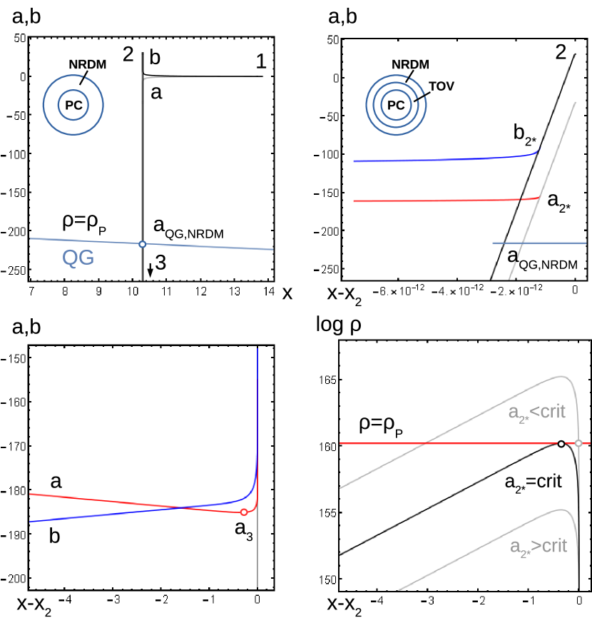
Figure 5: Solutions with NRDM, TOV and PC (Planck core) phases. See text for details.

Table 1: NRDM|TOV-star, stellar mass, critical case

model parameters	$M=10M_{\odot}$, $r_{s}=29532.4$m, $\epsilon=10^{-14}$
starting point	$a_{1}=0$, $b_{1}=0.0299773$,
of integration	$r_{1}=10^{6}$m, $L_{1}=1.05738\cdot 10^{6}$m
supershift	$a_{2}=-32.2362$, $b_{2}=30.8799$,
begins	$r_{2}/r_{s}-1=5.26127\cdot 10^{-7}$, $L_{2}=5.819\cdot 10^{-3}$m
NRDM|TOV	$a_{2*}=-154.936$, $b_{2*}=-90.434$,
transition	$r_{2*}/r_{2}-1=-1.2\cdot 10^{-12}$, $L_{2*}=1.32074\cdot 10^{-29}$m
supershift	$a_{3}=-185.052$, $b_{3}=-182.216$,
ends	$r_{3}=20638$m, $L_{3}=3.01835\cdot 10^{-36}$m
minimal radius,	$a_{4}=-95.1895$, $b_{4}=-272.808$,
end of integration	$r_{4}=l_{P}=1.62\cdot 10^{-35}$m, $L_{4}=0$

Table 2: various scenarios, global parameters

NRDM, $E_{in}=E_{P}$, $\lambda_{in}=l_{P}$
$M=10M_{\odot}$, $\epsilon=10^{-12}$	$A_{QG}=1.2\cdot 10^{-92}$, $\lambda_{out}=4.8\cdot 10^{-6}$pc
$M=10M_{\odot}$, $\epsilon=10^{-16}$	$A_{QG}=1.2\cdot 10^{-96}$, $\lambda_{out}=4.8\cdot 10^{-4}$pc
$M=4.06\cdot 10^{6}M_{\odot}$, $\epsilon=10^{-7}$	$A_{QG}=7.2\cdot 10^{-99}$, $\lambda_{out}=6.2\cdot 10^{-3}$pc
$M=4.06\cdot 10^{6}M_{\odot}$, $\epsilon=10^{-10}$	$A_{QG}=7.2\cdot 10^{-102}$, $\lambda_{out}=0.2$pc
NRDM|TOV critical, $E_{in}=0.512$MeV, $\lambda_{in}=2.42\cdot 10^{-12}$m
$M=10M_{\odot}$, $\epsilon=10^{-12}$	$A_{2*}=5.15\cdot 10^{-70}$, $\lambda_{out}=3.46$Mpc
$M=10M_{\odot}$, $\epsilon=10^{-14}$	$A_{2*}=5.15\cdot 10^{-68}$, $\lambda_{out}=0.346$Mpc
$M=10M_{\odot}$, $\epsilon=10^{-16}$	$A_{2*}=5.15\cdot 10^{-66}$, $\lambda_{out}=0.0346$Mpc
$M=4.06\cdot 10^{6}M_{\odot}$, $\epsilon=10^{-7}$	$A_{2*}=2.97\cdot 10^{-86}$, $\lambda_{out}=4.56\cdot 10^{5}$Gpc$\gg R_{uni}$
$M=4.06\cdot 10^{6}M_{\odot}$, $\epsilon=10^{-10}$	$A_{2*}=2.94\cdot 10^{-83}$, $\lambda_{out}=1.45\cdot 10^{4}$Gpc$\gg R_{uni}$

We numerically solve these equations using Mathematica NDSolve algorithm. As noted in [1], TOV systems are characterized by critical phenomena, abrupt changes in the solution with continuous change in parameters. As a result, the NRDM|TOV system has a richer solution structure than a pure NRDM.

Fig.5 shows the solution for a compact object of stellar mass $M=10M_{\odot}$. At the same time, as the study of the rotation curves [1] shows, the parameter $\epsilon$ for the external NRDM phase can be chosen in the interval $10^{-12...-16}$, and here we choose it in the center of this interval : $\epsilon=10^{-14}$.

The top left image shows the behavior of a pure NRDM solution, similar to the graphs from [1] for a supermassive solution. The solution starts at point 1, located at a large distance from the object, in the weak field region. Then, near the gravitational radius, the solution tries to enter the Schwarzschild mode with symmetrically diverging $a$ and $b$ profiles. The $b$ profile reaches its maximum at point 2, which is very close to the Schwarzschild radius $r_{s}$. After passing point 2, the solution goes into the supershift or mass inflation mode [52]. In a thin layer near this point, the $a$ and $b$ profiles rapidly decrease with decreasing $x$, while the mass density rapidly increases. At the point $a_{QG}$, the mass density reaches the Planck value. At this point, the NRDM phase joins the Planck core (PC). We recall that in the models under consideration, the Planck core has a large effectively negative mass due to quantum effects. This mass produces a force of gravitational repulsion, which maintains in equilibrium a coat of large positive mass located in the supershift region. These two masses almost cancel each other out, so that the object as a whole has an initial stellar mass.

The top right image shows the modification of the solution when it is connected with the TOV phase. The $a$ and $b$ profiles rapidly falling in a thin $x$-layer of the NRDM phase, before passing the Planck boundary and after crossing the $2*$ phase boundary, are replaced by more slowly falling TOV phase profiles. In the figure at the bottom left, the TOV solution is continued into a wider $x$-layer. At point 3, the solution passes through the minimum of the $a$ profile. Further, the profiles $a$ and $b$ diverge symmetrically in the region of large negative values, which is typical for the Schwarzschild singularity of negative mass [50] Sec.28.5. Unlike other known solutions, this singularity is not naked, it is covered with a massive coat and remains in the superstrong redshift zone until the integration stops at the Planck radius.

The figure at the bottom right shows the behavior of the mass density of the solution in the TOV phase. The maximum density is reached at the minimum point $a_{3}$. The critical solution, which touches the Planck density line, is specially highlighted. For this solution, all the other TOV graphs in this figure are shown. The key parameters for this solution are also listed in Table 1.

Upon reaching the Planck density, the solution joins the Planck core. In supercritical mode, that is, when the point of joining of the phases $a_{2*}$ is selected below the critical position, the density reaches the Planck value earlier, the boundary of the Planck core shifts accordingly.

In subcritical mode, the Planck density is not reached at all, and the solution continues until the central singularity. This singularity is quite similar to the Planck core, since it also has a large negative mass, and its repulsive force keeps the system in equilibrium. The singularity can be smeared over the $r\sim l_{P}$ neighborhood to obtain a regular core. One can also expand the core to larger radius values. We will call such solutions the Planck core of type II, in contrast to the previously considered solutions, to which we assign the type I. Their difference is that core I arises when the NRDM or TOV matter reaches the Planck density, while for core II the density of this matter remains sub-Planckian, and the core consists of other matter exceeding the Planck density. NRDM solutions for the physically relevant selection of parameters necessarily exceed the Planck density, so a type I core is formed there. For the TOV phase, both types of solutions are possible.

Wavelengths

of photons in the resulting gravitational field are easy to calculate. The initial wavelength, which was equal to $\lambda_{in}=l_{P}$ on the surface of the Planck core for the NRDM solution, is replaced by $E_{in}=0.512$MeV, $\lambda_{in}=2.42\cdot 10^{-12}$m at the interface for the NRDM|TOV solution. This choice corresponds to the threshold for the production of $e^{+}e^{-}$ pairs in the collision of incoming and outgoing photon fluxes. An ultrarelativistic TOV plasma is composed of these pairs and other higher-energy particles. Applying the redshift to this wavelength for the critical case $A_{2*}=5.15\cdot 10^{-68}$ from Table 1, we get $\lambda_{out}=\lambda_{in}/\sqrt{A_{2*}}=1.07\cdot 10^{22}$m $=0.346$Mpc. In the supercritical mode, longer wavelengths are obtained, in the subcritical mode, shorter ones. Note the coincidence of the obtained wavelength with the characteristic size of the MW galaxy. This coincidence is even more surprising if we note that the metric coefficients appearing in the intermediate calculations vary in the considered solutions by a hundred orders of magnitude.

L-integral.

Table 1 also lists the values of the invariant length integral measured in the radial direction: $L=\int dr\sqrt{B}$. Integration starts from the minimum radius $r=l_{P}$. The integral up to point 3 turns out to be less than the Planck length, which does not pose a problem, since this region contains a Planck core with unknown properties, and the integration over this region should not be carried out at all. The integral up to point $2*$ represents the thickness of the TOV layer. It is noteworthy that in the $r$-coordinate this thickness is about 9km, while in the $L$-coordinate this thickness is microscopic: $L_{2*}=8\cdot 10^{5}l_{P}$. This difference is an indicator of a strong deformation of the radial direction in the solution, which manifests itself in an extremely small $B$-factor. Note that the “aerial” $r$-coordinate is related to the area of the corresponding sphere (always equal to $4\pi r^{2}$), while the $L$-coordinate is the more appropriate local thickness characteristic. The resulting thin layer corresponds to a superdense TOV plasma sandwiched between the Planck core and NRDM coat under tremendous pressure. We remind that in our calculations we consider all the media to be continuous, disregarding their microscopic structure. Apparently, a quantum calculation should be carried out in this region, after which the results obtained here should be revised. In this work, we restrict ourselves to classical calculations. Further, up to point 2, the coordinate $r$ changes microscopically by $\sim 3.5\cdot 10^{-8}$m, while the change in $L$ is about 6mm. In this region, the deformation becomes inverse, due to the large $B$-factor near point 2. Finally, in the outer region, an $L$-integral is accumulated, comparable to the change in $r$, since the region of weak fields prevails here, and the space becomes flat.

The picture obtained in the analysis of the $L$-integral coincides with the structure of compact massive objects and the presence of a “shrinking volume” [3] inside them. In the region shallow in the $L$-coordinate, thin superdense layers of matter are localized, creating strong deformations of space, strong gravitational fields that determine the structure of the solution as a whole.

Sensitivity to model parameters.

Table 2 shows the calculation results for different scenarios. For a pure NRDM model, the value of $\lambda_{out}$ varies in the range of $10^{11...16}$m or $10^{-6...-1}$pc. If the DM particles in this scenario were photons, their propagation in the ISM would be prohibited, since their frequency is significantly less than Langmuir’s value and the wavelength is significantly less than the size of the galaxy. However, this scenario is limited to the sterile case and does not consider photons as DM particles. The photon case assumes an NRDM|TOV combination, and here, for compact objects of stellar mass, wavelengths are obtained in the range of 34.6kpc-3.46Mpc, that is, comparable to galactic sizes. We assume that such waves can propagate in ISM and condense in BEC, thereby providing a logical closure for the considered model. For the supermassive case, typical for central black holes in galaxies, $\lambda_{out}$ values are obtained that are much larger than the size of the universe $R_{uni}\sim 14$Gpc. This means that either supermassive black holes in this scenario do not participate in the formation of dark matter, or cosmological processes must be taken into account for their analysis. Note also that in the case of a pure NRDM for the described parameters there are exact formulas: $A_{QG}=\epsilon(l_{P}/r_{s})^{2}/(8\pi)$, $\lambda_{out}=r_{s}(8\pi/\epsilon)^{1/2}$. For the NRDM|TOV combination, we currently have only empirical relationships. Namely, for the data in Table 2, with fixed $r_{s}$ and variable $\epsilon$, the relations hold $A_{2*}\sim\epsilon^{-1}$, $B_{2*}\sim\epsilon^{-3}$, $\lambda_{out}\sim\epsilon^{1/2}$, which are the sign of hidden symmetries in the considered system.

Qualitative analysis.

At the first glance, the presented results are relevant only to the model of NRDM|TOV stars studied here. Now we will show that many features of the described solution are typical for a wider class of models, possibly for all compact massive objects [2, 3, 4, 5]. First of all, erasure of the event horizon is associated with the T-symmetry of solutions, which results in a grid of the intersecting flows of incoming and outgoing particles. For true black holes, there are only incoming flows, and for T-conjugated white holes, only outgoing flows. In the solutions under consideration, there can be no horizons that could prevent the entry or exit of the particles. Another explanation for the horizon erasure effect arises when observing the mass function $M(r)$. The region below the horizon corresponds to $2M(r)/r>1$. In the presence of distributed positive mass density, the function $M(r)$ decreases with decreasing $r$ (one can imagine how positive mass layers are removed from the solution). If the density is high enough, then $2M(r)$ decreases faster than $r$, so no horizon is formed. High density arises from the phenomenon of mass inflation [52]. This phenomenon occurs due to the positive feedback between pressure and gravity. In strong gravitational fields, in equilibrium systems, the pressure increases rapidly with decreasing radius, due to the hydrostatic equation. At high pressure, it begins to contribute to gravity on the same basis as mass density, which also increases due to EOS. As a result, the gravitational field is strengthened, which leads to a further increase in pressure and density. As a result, a thin layer is formed in the solution, in which pressure, density and gravitational field increase very rapidly. Further, the rapid decrease in the mass function $M(r)$ does not stop at zero crossing, the mass becomes negative. While the local density is still positive, the value of the central mass located under a certain radius $r$ is negative. A successful closure of the model is the concept of the Planck core, according to which, when the Planck density is exceeded, the quantum corrections make the mass effectively negative [4, 5]. We described another possibility in this work, when a central singularity or a superdense core, consisting of matter other than the surrounding massive coat, has a negative mass. Next, we observe the behavior of the metric profiles $A$ and $B$, where the first describes the time dilation and redshift, and the second describes the deformation of the radial coordinate. The mass function is directly related to the $B$-profile by the formula $B=(1-2M/r)^{-1}$. Large negative masses correspond to a small positive $B$. As a result, the integral of length $L=\int dr\sqrt{B}$ in this region becomes small, the region becomes shallow in $L$, although in $r$ it can occupy an essential part of the solution. Together with the coefficient $B$, $A$ also becomes small in the region of mass inflation, which is typical for strong gravitational fields. This leads to a strong time dilation and redshift, as a result, from the point of view of an external observer, the object is dark, almost like a black hole. At the same time, high energies inside the object can result in high density radiation. The redshift does not affect the flux density in the transverse direction and shifts the radiation to the low-energy region. In the models under consideration, the superstrong redshift stretches photons into ultra-long wave packets that can reach the size of a galaxy, while a large number of such photons, after taking into account all sources, leads to a significant contribution to the mass of the galaxy. Thus, microscopically thin high-energetic layers inside compact objects appear to be conjugated with galactic-scale structures. At large distances from the center, the radiation density decreases as $\rho\sim r^{-2}$, which leads to flat rotation curves of galaxies. The distribution of black holes in the galaxy modulates these dependencies and allows to describe the observed rotation curves with their deviations from the flat shape [1]. These calculations do not depend on the nature of the emitting objects, only on the assumption that their distribution is proportional to the luminous matter. Thus, radiation from compact massive objects, be they photons or other particles, may be directly unobservable due to long wavelengths. However, it can determine the rotation curves of galaxies and produce other gravitational effects that are usually associated with dark matter. If this type of radiation can pass the interstellar medium and become Bose-Einstein condensate outside the galaxy, one will simultaneously obtain the description of dark energy.

4 Conclusion

This work continued the construction of a recently proposed model of NRDM-stars. In this model, the quanta dark of matter are sterile massless particles that are emitted from quasi-black holes located mainly in the central regions of the galaxy. At large distances from the center of the galaxy, the emission is directed radially and the mass density has the form $\rho\sim r^{-2}$, in contrast to the homogeneous model $\rho=Const$. In the cosmological context, the homogeneous model with massless particles corresponds to the radiation epoch of the expansion of the universe, while the proposed inhomogeneous model turns out to be equivalent to $\Lambda$CDM.

Specifically, several scenarios were considered in which the radial emission of dark matter is brought into hydrostatic equilibrium with a uniform background:

• a jump in the dark energy density at the edge of the galactic halo;

• a surface tension at the boundary between the halo and the dark energy background;

• a phase transition of dark matter into dark energy, accompanied by the Joule-Thomson effect;

• Bose-Einstein condensation of dark matter inside the galaxy into dark energy outside of it.

From the junction conditions, the density correspondence to the observed $\Omega$-parameters and mass functions typical for $\Lambda$CDM model were obtained. In these scenarios, CDM macro-particles are galaxies with massive halos surrounding them, floating in a homogeneous medium with the dark energy equation of state.

Additionally, the question of what happens if dark matter particles are not sterile, for example, are photons of the Standard Model, is considered. When high-energy photons collide inside NRDM stars, as a result of the production of $e^{+}e^{-}$ pairs and other particles, a thin layer of ultrarelativistic plasma appears. The performed classical calculation shows that the photons emitted from this layer, after applying the gravitational redshift, acquire a wavelength comparable to the galactic sizes. For the logical closure of the photon scenario in this model, it is also necessary to study the questions of the passage of such longwave photons through the interstellar medium and Bose-Einstein condensation of the photons in the intergalactic medium. The study of these questions will be continued.

References

- [1] I. Nikitin: On dark stars, Planck cores and the nature of dark matter, Bled Workshops in Physics 21, 221-246 (2020); arXiv:2102.07769.
- [2] M. Visser, C. Barceló, S. Liberati, S. Sonego: Small, dark, and heavy: But is it a black hole?, Proc. of Science 075, Black Holes in General Relativity and String Theory, 010 (2008); arXiv:0902.0346.
- [3] B. Holdom, J. Ren: Not quite a black hole, Phys. Rev. D95, 084034 (2017); arXiv:1612.04889.
- [4] C. Rovelli, F. Vidotto: Planck stars, Int. J. Mod. Phys. D23, 1442026 (2014); arXiv:1401.6562.
- [5] C. Barceló, R. Carballo-Rubio, L. J. Garay, G. Jannes: The lifetime problem of evaporating black holes: mutiny or resignation, Class. Quantum Grav. 32, 035012 (2015); arXiv:1409.1501.
- [6] R. Brandenberger, J. Fröhlich, R. Namba: Unified dark matter, dark energy and baryogenesis via a “cosmological wetting transition”, J. of Cosmology and Astroparticle Phys. 2019, 069 (2019); arXiv:1907.06353.
- [7] C. Wetterich: Cosmon dark matter?, Phys. Rev. D65, 123512 (2002); arXiv:hep-ph/0108266.
- [8] A. Banihashemi, N. Khosravi, A. H. Shirazi: Ups and downs in dark energy: phase transition in dark sector as a proposal to lessen cosmological tensions, Phys. Rev. D101, 123521 (2020); arXiv:1808.02472.
- [9] A. Banihashemi, N. Khosravi, A. Shafieloo: Dark energy as a critical phenomenon: a hint from Hubble tension, J. of Cosmology and Astroparticle Phys. 2021, 003 (2021); arXiv:2012.01407.
- [10] J.-P. Hong, S. Jung, K.-P. Xie: Fermi-ball dark matter from a first-order phase transition, Phys. Rev. D102, 075028 (2020); arXiv:2008.04430.
- [11] M. J. Baker, J. Kopp, A. J. Long: Filtered dark matter at a first order phase transition, Phys. Rev. Lett. 125, 151102 (2020); arXiv:1912.02830.
- [12] E. Hall, T. Konstandin, R. McGehee, H. Murayama: Asymmetric matters from a dark first-order phase transition, Report IPMU19-0171, DESY19-209; arXiv:1911.12342.
- [13] K. Ghorbani, P. H. Ghorbani: A simultaneous study of dark matter and phase transition: two-scalar scenario, J. of High Energy Phys, 2019, 77 (2019); arXiv:1906.01823.
- [14] G. Chapline: Dark energy stars, Proc. of the Texas Conference on Relativistic Astrophysics, Stanford, CA, December, 2004; arXiv:astro-ph/0503200.
- [15] G. Chapline, E. Hohlfeld, R. B. Laughlin, D. I. Santiago: Quantum phase transitions and the breakdown of classical general relativity, Int. J. Mod. Phys. A18, 3587-3590 (2003); arXiv:gr-qc/0012094.
- [16] A. B. Balakin, A. S. Ilin: Dark energy and dark matter interaction: kernels of Volterra type and coincidence problem, Symmetry 10, 411 (2018); arXiv:1809.05678.
- [17] W. Yang, N. Banerjee, A. Paliathanasis, S. Pan: Reconstructing the dark matter and dark energy interaction scenarios from observations, Phys. Dark Univ. 26, 100383 (2019); arXiv:1812.06854.
- [18] G. Cheng, Y.-Z. Ma, F. Wu, J. Zhang, X. Chen: Testing interacting dark matter and dark energy model with cosmological data, Phys. Rev. D102, 043517 (2020); arXiv:1911.04520.
- [19] A. Paliathanasis, S. Pan, W. Yang: Dynamics of nonlinear interacting dark energy models, Int. J. Mod. Phys. D28, 1950161 (2019); arXiv:1903.02370.
- [20] Z. Rezaei: Dark matter – dark energy interaction and the shape of cosmic voids, The Astrophys. J. 902, 102 (2020); arXiv:2010.10823.
- [21] M. Lucca, D. C. Hooper: Tensions in the dark: shedding light on dark matter – dark energy interactions, Phys. Rev. D102, 123502 (2020); arXiv:2002.06127.
- [22] W. Yang, S. Pan, A. Paliathanasis: Cosmological constraints on an exponential interaction in the dark sector, Mon. Not. Roy. Astron. Soc. 482, 1007-1016 (2019); arXiv:1804.08558.
- [23] V. H. Cárdenas, D. Grandón, S. Lepe: Dark energy and dark matter interaction in light of the second law of thermodynamics, The European Phys. J. C79, 357 (2019); arXiv:1812.03540.
- [24] S. Pan, W. Yang, E. Di Valentino, A. Shafieloo, S. Chakraborty: Reconciling tension in a six parameter space?, J. of Cosmology and Astroparticle Phys. 2020, 062 (2020); arXiv:1907.12551.
- [25] X. Li, A. Shafieloo: Evidence for emergent dark energy, The Astrophys. J. 902, 58 (2020); arXiv:2001.05103.
- [26] E. Di Valentino, A. Melchiorri, O. Mena, S. Vagnozzi: Interacting dark energy in the early 2020s: a promising solution to the and cosmic shear tensions, Phys. Dark Univ. 30, 100666 (2020); arXiv:1908.04281.
- [27] E. Di Valentino, A. Melchiorri, O. Mena, S. Vagnozzi: Non-minimal dark sector physics and cosmological tensions, Phys. Rev. D101, 063502 (2020); arXiv:1910.09853.
- [28] E. Di Valentino, O. Mena: A fake interacting dark energy detection?, Mon. Not. Roy. Astron. Soc. Lett. 500, L22-L26 (2021); arXiv:2009.12620.
- [29] K. L. Pandey, T. Karwal, S. Das: Alleviating the and anomalies with a decaying dark matter model, J. of Cosmology and Astroparticle Phys. 2020, 026 (2020); arXiv:1902.10636.
- [30] S. Ghosh, R. Khatri, T. S. Roy: Dark neutrino interactions phase out the Hubble tension, Phys. Rev. D102, 123544 (2020); arXiv:1908.09843.
- [31] S. Pan, W. Yang, A. Paliathanasis: Nonlinear interacting cosmological models after Planck 2018 legacy release and the tension, Mon. Not. Roy. Astron. Soc. 493, 3114-3131 (2020); arXiv:2002.03408.
- [32] S. Panpanich, P. Burikham, S. Ponglertsakul, L. Tannukij: Resolving Hubble tension with quintom dark energy model, Chin. Phys. C45 (2021) 015108; arXiv:1908.03324.
- [33] M. Archidiacono, D. C. Hooper, R. Murgia, S. Bohr, J. Lesgourgues, M. Viel: Constraining dark matter – dark radiation interactions with CMB, BAO, and Lyman-, J. of Cosmology and Astroparticle Phys. 2019, 055 (2019); arXiv:1907.01496.
- [34] M. Martinelli, I. Tutusaus: CMB Tensions with low-redshift and measurements: impact of a redshift-dependent type-Ia supernovae intrinsic luminosity, Symmetry 11, 986 (2019); arXiv:1906.09189.
- [35] G.-B. Zhao et al.: Dynamical dark energy in light of the latest observations, Nature Astronomy 1, 627-632 (2017); arXiv:1701.08165.
- [36] Y. Wang, L. Pogosian, G.-B. Zhao, A. Zucca: Evolution of dark energy reconstructed from the latest observations, The Astrophys. J. Lett. 869, L8 (2018); arXiv:1807.03772.
- [37] E. Castellanos, C. Escamilla-Rivera: Dark energy as generalised superfluid excitations; arXiv:2006.06129.
- [38] E. G. M. Ferreira: Unified superfluid dark sector, in: Quantum Theory and Symmetries, CRM Series in Mathematical Physics, Springer 2021; arXiv:1911.07371.
- [39] K. Huang: Dark energy and dark matter in a superfluid universe, Int. J. Mod. Phys. A28, 1330049 (2013); arXiv:1309.5707.
- [40] J.-W. Lee, I.-G. Koh: Galactic halos as boson stars, Phys. Rev. D53, 2236-2239 (1996); arXiv:hep-ph/9507385.
- [41] E. Braaten, A. Mohapatra, H. Zhang: Dense axion stars; Phys. Rev. Lett. 117, 121801 (2016); arXiv:1512.00108.
- [42] L. Visinelli, S. Baum, J. Redondo, K. Freese, F. Wilczek: Dilute and dense axion stars, Phys. Lett. B777, 64-72 (2018); arXiv:1710.08910.
- [43] V. A. Popov: Dark energy and dark matter unification via superfluid Chaplygin gas, Phys. Lett. B686, 211-215 (2010); arXiv:0912.1609.
- [44] Y. Sofue, V. C. Rubin: Rotation curves of spiral galaxies, Ann. Rev. Astron. Astrophys. 39, 137-174 (2001); arXiv:astro-ph/0010594.
- [45] Y. Sofue, M. Honma, T. Omodaka: Unified rotation curve of the Galaxy – decomposition into de Vaucouleurs bulge, disk, dark halo, and the 9-kpc rotation dip, Publications of the Astronomical Society of Japan 61, 227-236 (2009); arXiv:0811.0859.
- [46] Y. Sofue: Pseudo rotation curve connecting the Galaxy, dark halo, and Local Group, Publications of the Astronomical Society of Japan 61, 153-161 (2009); arXiv:0811.0860.
- [47] Y. Sofue: A grand rotation curve and dark matter halo in the Milky Way galaxy, Publications of the Astronomical Society of Japan 64, 75 (2012); arXiv:1110.4431.
- [48] Y. Sofue: Rotation curve and mass distribution in the Galactic Center – from black hole to entire Galaxy, Publications of the Astronomical Society of Japan 65, 118 (2013); arXiv:1307.8241.
- [49] S. Dodelson: Modern Cosmology, Elsevier, 2003.
- [50] M. Blau: Lecture Notes on General Relativity, University of Bern, 2021, www.blau.itp.unibe.ch/newlecturesGR.pdf
- [51] A. Kruchkov, Yu. Slyusarenko: Bose-Einstein condensation of photons in an ideal atomic gas, Phys. Rev. A88, 013615 (2013); arXiv:1305.1210.
- [52] A. J. S. Hamilton, S. E. Pollack: Inside charged black holes: II. Baryons plus dark matter, Phys. Rev. D71, 084032 (2005), arXiv:gr-qc/0411062.
- [53] F. Sylos Labini, M. Montuori, L. Pietronero: Scale-invariance of galaxy clustering, Phys. Rep. 293, 61-226 (1998); arXiv:astro-ph/9711073.
- [54] J. Peñarrubia, Yin-Zhe Ma, M. G. Walker, A. McConnachie: A dynamical model of the local cosmic expansion, Mon. Not. Roy. Astron. Soc. 443, 2204-2222 (2014); arXiv:1405.0306.
- [55] J. Barranco, A. Bernal, D. Nunez: Dark matter equation of state from rotational curves of galaxies, Mon. Not. Roy. Astron. Soc. 449, 403 (2015), arXiv:1301.6785.
- [56] C. J. Conselice, A. Wilkinson, K. Duncan, A. Mortlock: The evolution of galaxy number density at and its implications, The Astrophys. J. 830, 83 (2016); arXiv:1607.03909.
- [57] T. C. Licquia, J. A. Newman: Improved estimates of the Milky Way’s stellar mass and star formation rate from hierarchical Bayesian meta-analysis, The Astrophys. J. 806, 96 (2015); arXiv:1407.1078.
- [58] A. G. Bedregal, A. Aragón-Salamanca, M. R. Merrifield: The Tully-Fisher relation for S0 galaxies, Mon. Not. Roy. Astron. Soc. 373, 1125-1140 (2006); arXiv:astro-ph/0609076.
- [59] R. Schaeffer, S. Maurogordato, A. Cappi, F. Bernardeau: The fundamental plane of galaxy clusters, Mon. Not. Roy. Astron. Soc. 263, L21-L26 (1993); arXiv:astro-ph/9304018.
- [60] M. Girardi, P. Manzato, M. Mezzetti, G. Giuricin, F. Limboz: Observational mass-to-light ratio of galaxy systems from poor groups to rich clusters, The Astrophys. J. 569, 720 (2002).
- [61] P. Salucci et al.: The universal rotation curve of spiral galaxies. II. The dark matter distribution out to the virial radius, Mon. Not. Roy. Astron. Soc. 378, 41-47 (2007); arXiv:astro-ph/0703115.
- [62] E. V. Karukes, P. Salucci: The universal rotation curve of dwarf disk galaxies, Mon. Not. Roy. Astron. Soc. 465, 4703-4722 (2017); arXiv:1609.06903.
- [63] M. Visser: Lorentzian Wormholes: from Einstein to Hawking, Springer, 1996.
- [64] J. B. Hartle: Gravity: An Introduction to Einstein’s General Relativity, Addison-Wesley, 2003.