Divergence-Regularized Multi-Agent Actor-Critic

Abstract

Entropy regularization is a popular method in reinforcement learning (RL). Although it has many advantages, it alters the RL objective of the original Markov Decision Process (MDP). Though divergence regularization has been proposed to settle this problem, it cannot be trivially applied to cooperative multi-agent reinforcement learning (MARL). In this paper, we investigate divergence regularization in cooperative MARL and propose a novel off-policy cooperative MARL framework, divergence-regularized multi-agent actor-critic (DMAC). Theoretically, we derive the update rule of DMAC which is naturally off-policy and guarantees monotonic policy improvement and convergence in both the original MDP and divergence-regularized MDP. We also give a bound of the discrepancy between the converged policy and optimal policy in the original MDP. DMAC is a flexible framework and can be combined with many existing MARL algorithms. Empirically, we evaluate DMAC in a didactic stochastic game and StarCraft Multi-Agent Challenge and show that DMAC substantially improves the performance of existing MARL algorithms.

1 Introduction

Regularization is a common method for single-agent reinforcement learning (RL). The optimal policy learned by traditional RL algorithms is always deterministic (Sutton & Barto, 2018). This property may result in the inflexibility of the policy facing unknown environments (Yang et al., 2019). Entropy regularization is proposed to settle this problem by learning a policy according to the maximum-entropy principle (Haarnoja et al., 2017). Moreover, entropy regularization is beneficial to exploration and robustness for RL algorithms (Haarnoja et al., 2018). However, entropy regularization is imperfect. Eysenbach & Levine (2019) pointed out that maximum-entropy RL modifies the original RL objective because of the entropy regularizer. Maximum-entropy RL is actually learning an optimal policy for the entropy-regularized Markov Decision Process (MDP) rather than the original MDP, i.e., the converged policy may be biased. Nachum et al. (2017) analyzed a more general case for regularization in RL and proposed what we call divergence regularization. Divergence regularization is beneficial to exploration and may be helpful to the bias issue.

Regularization can also be applied to cooperative multi-agent reinforcement learning (MARL) (Agarwal et al., 2020; Zhang et al., 2021). However, most cooperative MARL algorithms do not use regularizers (Lowe et al., 2017; Foerster et al., 2018; Rashid et al., 2018; Son et al., 2019; Jiang et al., 2020; Wang et al., 2021a). Only few cooperative MARL algorithms such as FOP (Zhang et al., 2021) use entropy regularization, which may suffer from the drawback aforementioned. Divergence regularization, on the other hand, could potentially benefit cooperative MARL. In addition to its advantages mentioned above, divergence regularization can also help to control the step size of policy update which is similar to conservative policy iteration (Kakade & Langford, 2002) in single-agent RL. Conservative policy iteration and its successive methods such as TRPO (Schulman et al., 2015) and PPO (Schulman et al., 2017) can stabilize policy improvement (Touati et al., 2020). These methods use a surrogate objective for policy update, but the policies in centralized training with decentralized execution (CTDE) paradigm may not preserve the properties of the surrogate objective. Moreover, DAPO (Wang et al., 2019), a single-agent RL algorithm using divergence regularizer, cannot be trivially extended to cooperative MARL settings. Even with some tricks like V-trace (Espeholt et al., 2018) for off-policy correction, DAPO is essentially an on-policy algorithm and thus may not be sample-efficient in cooperative MARL settings.

In the paper, we propose divergence-regularized multi-agent actor-critic (DMAC), a novel off-policy cooperative MARL framework. We analyze the general iteration of DMAC and theoretically show that DMAC guarantees the monotonic policy improvement and convergence in both the original MDP and the divergence-regularized MDP. We also derive a bound of the discrepancy between the converged policy and the optimal policy in the original MDP. Besides, DMAC is beneficial to exploration and stable policy improvement by applying our update rule of target policy. We also propose and analyze divergence policy iteration in general cooperative MARL settings and a special case combined with value decomposition. Based on divergence policy iteration, we derive the off-policy update rule for the critic, policy, and target policy. Moreover, DMAC is a flexible framework and can be combined with many existing cooperative MARL algorithms to substantially improve their performance.

We empirically investigate DMAC in a didactic stochastic game and StarCraft Multi-Agent Challenge (Samvelyan et al., 2019). We combine DMAC with five representative MARL methods, i.e., COMA (Foerster et al., 2018) for on-policy multi-agent policy gradient, MAAC (Iqbal & Sha, 2019) for off-policy multi-agent actor-critic, QMIX (Rashid et al., 2018) for value decomposition, DOP (Wang et al., 2021b) for the combination of value decomposition and policy gradient, and FOP (Zhang et al., 2021) for the combination of value decomposition and entropy regularization. Experimental results show that DMAC indeed induces better performance, faster convergence, and better stability in most tasks, which verifies the benefits of DMAC and demonstrates the advantages of divergence regularization over entropy regularization in cooperative MARL.

2 Related Work

MARL. MARL has been a hot topic in the field of RL. In this paper, we focus on cooperative MARL. Cooperative MARL is usually modeled as Dec-POMDP (Oliehoek et al., 2016), where all agents share a reward and aim to maximize the long-term return. Centralized training with decentralized execution (CTDE) (Lowe et al., 2017) paradigm is widely used in cooperative MARL. CTDE usually utilizes a centralized value function to address the non-stationarity for multi-agent settings and decentralized policies for scalability. Many MARL algorithms adopt CTDE paradigm such as COMA, MAAC, QMIX, DOP, and FOP. COMA (Foerster et al., 2018) employs the counterfactual baseline which can reduce the variance as well as settle the credit assignment problem. MAAC (Iqbal & Sha, 2019) uses self-attention mechanism to integrate local observation and action of each agent and provides structured information for the centralized critic. Value decomposition (Sunehag et al., 2018; Rashid et al., 2018; Son et al., 2019; Yang et al., 2020; Wang et al., 2021a, b; Zhang et al., 2021; Sun et al., 2021; Pan et al., 2021; Peng et al., 2021) is a popular class of cooperative MARL algorithms. These methods express the global Q-function as a function of individual Q-functions to satisfy Individual-Global-Max (IGM), which means the optimal actions of individual Q-functions are corresponding to the optimal joint action of the global Q-function. QMIX (Rashid et al., 2018) is a representative of value decomposition methods. It uses a hypernet to ensure the monotonicity of the global Q-function in terms of individual Q-functions, which is a sufficient condition of IGM. DOP (Wang et al., 2021b) is a method that combines value decomposition with policy gradient. DOP uses a linear value decomposition which is another sufficient condition of IGM and the linear value decomposition helps the compute of policy gradient. FOP (Zhang et al., 2021) is a method that combines value decomposition with entropy regularization and uses a more general condition, Individual-Global-Optimal, to replace IGM. In this paper, we will combine DMAC with these algorithms and show its improvement. MAPPO (Yu et al., 2021) is a CTDE version of PPO (Schulman et al., 2017), where a centralized state-value function is learned. However, the update rule of policy of MAPPO contradicts DMAC, so DMAC cannot be combined with MAPPO.

Regularization. Entropy regularization was first proposed in single-agent RL. Nachum et al. (2017) analyzed the entropy-regularized MDP and revealed the properties about the optimal policy and the corresponding Q-function and V-function. They also showed the equivalence of value-based methods and policy-based methods in entropy-regularized MDP. Haarnoja et al. (2018) pointed out maximum-entropy RL can achieve better exploration and stability facing the model and estimation error. Although entropy regularization has many advantages, Eysenbach & Levine (2019) showed entropy regularization modifies the MDP and results in the bias of the convergent policy. Yang et al. (2019) revealed the drawbacks of the convergent policy of general RL and maximum-entropy RL. The former is usually a deterministic policy (Sutton & Barto, 2018) that is not flexible enough for unknown situations, while the latter is a policy with non-zero probability for all actions which may be dangerous in some scenarios. Neu et al. (2017) analyzed the entropy regularization method from several views. They revealed a more general form of regularization which is actually divergence regularization and showed entropy regularization is just a special case of divergence regularization. Wang et al. (2019) absorbed previous results and proposed an on-policy algorithm, i.e., DAPO. However, DAPO cannot be trivially applied to MARL. Moreover, its on-policy learning is not sample-efficient for MARL settings, and its off-policy correction trick V-trace (Espeholt et al., 2018) is also intractable in MARL. There are some previous studies in single-agent RL which use similar target policy to ours, but their purposes are quite different. Trust-PCL (Nachum et al., 2018) introduces a target policy as a trust-region constraint for maximum-entropy RL, but the policy is still biased by entropy regularizer. MIRL (Grau-Moya et al., 2019) uses a distribution that is only related to actions as the target policy to compute a mutual-information regularizer, but it still changes the objective of the original RL.

3 Preliminaries

Dec-POMDP is a general model for cooperative MARL. A Dec-POMDP is a tuple $M=\left\{S,A,P,Y,O,I,n,r,\gamma\right\}$. $S$ is the state space, $n$ is the number of agents, $\gamma$ is the discount factor, and $I=\{1,2\cdots n\}$ is the set of all agents. $A=A_{1}\times A_{2}\times\cdots\times A_{n}$ represents the joint action space where $A_{i}$ is the individual action space for agent $i$. $P(s^{\prime}|s,\bm{a}):S\times A\times S\to[0,1]$ is the transition function, and $r(s,\bm{a}):S\times A\to\mathbb{R}$ is the reward function of state $s$ and joint action $\bm{a}$. $Y$ is the observation space, and $O(s,i):S\times I\to Y$ is a mapping from state to observation for each agent. The objective of Dec-POMDP is to maximize $J({\bm{\pi}})=\mathbb{E}_{\bm{\pi}}\left[\sum_{t=0}\gamma^{t}r(s_{t},\bm{a}_{t})\right],$ and thus we need to find the optimal joint policy ${\bm{\pi}}^{*}=\arg\max_{{\bm{\pi}}}J({\bm{\pi}})$. To settle the partial observable problem, history $\tau_{i}\in\mathcal{T}_{i}=(Y\times A_{i})^{*}$ is often used to replace observation $o_{i}\in Y$. As for policies in CTDE, each agent $i$ has an individual policy $\pi_{i}(a_{i}|\tau_{i})$ and the joint policy $\bm{\pi}$ is the product of each $\pi_{i}$. Though we calculate individual policy as $\pi_{i}(a_{i}|\tau_{i})$ in practice, we will use $\pi_{i}(a_{i}|s)$ in analysis and proofs for simplicity.

Entropy regularization adds the logarithm of the probability of the sampled action according to current policy to the reward function. It modifies the optimization objective as $J_{\operatorname{ent}}(\bm{\pi})=\mathbb{E}_{\bm{\pi}}\left[\sum_{t=0}\gamma^{t}\left(r(s_{t},\bm{a}_{t})-\omega\log\bm{\pi}(\bm{a}_{t}|s_{t})\right)\right].$ We also have the corresponding Q-function $Q_{\operatorname{ent}}^{\bm{\pi}}(s,\bm{a})=r(s,\bm{a})+\gamma\mathbb{E}\left[V_{\operatorname{ent}}^{\bm{\pi}}(s^{\prime})\right]$ and V-function $V_{\operatorname{ent}}^{\bm{\pi}}(s)=\mathbb{E}_{\bm{\pi}}\left[\sum_{t=0}\gamma^{t}\left(r(s_{t},\bm{a}_{t})-\omega\log\bm{\pi}(\bm{a}_{t}|s_{t})\right)|s_{0}=s\right]$. Given these definitions, we can deduce an interesting property $V_{\operatorname{ent}}^{\bm{\pi}}(s)=\mathbb{E}\left[Q_{\operatorname{ent}}^{\bm{\pi}}(s,\bm{a})\right]+\omega\mathcal{H}\left(\bm{\pi}(\cdot|s)\right)$, where $\mathcal{H}\left(\bm{\pi}(\cdot|s)\right)$ represents the entropy of policy $\bm{\pi}(\cdot|s)$. $V_{\operatorname{ent}}^{\bm{\pi}}(s)$ includes an entropy term which is the reason it is called entropy regularization.

4 Method

In this section, we first give the definition of divergence regularization. Then we propose the selection of target policy and derive its theoretical properties. Next we propose and analyze divergence policy iteration. Finally, we derive the update rules of the critic and actors and obtain the algorithm of DMAC. Note that all proofs are given in Appendix A.

4.1 Divergence Regularization

We maintain a target policy $\rho_{i}$ for each agent $i$, which is different from the agent policy $\pi_{i}$. Together we have a joint target policy ${\bm{\rho}}=\prod_{i=1}^{n}\rho_{i}$. This joint target policy ${\bm{\rho}}$ modifies the objective function as $J_{\bm{\rho}}({\bm{\pi}})=\mathbb{E}_{\bm{\pi}}\left[\sum_{t=0}\gamma^{t}\left(r(s_{t},\bm{a}_{t})-\omega\log\frac{{\bm{\pi}}(\bm{a}_{t}|s_{t})}{{\bm{\rho}}(\bm{a}_{t}|s_{t})}\right)\right].$ That is, a regularizer $\log\frac{{\bm{\pi}}(\bm{a}_{t}|s_{t})}{{\bm{\rho}}(\bm{a}_{t}|s_{t})}$, which describes the discrepancy between policy ${\bm{\pi}}$ and target policy ${\bm{\rho}}$, is added to the reward function just like entropy regularization.

Given $\bm{\rho}$, we can define the corresponding V-function and Q-function for divergence regularization as follows,

$$V_{\bm{\rho}}^{{\bm{\pi}}}(s)=\mathbb{E}_{\bm{\pi}}\left[\sum_{t=0}\gamma^{t}(r(s_{t},\bm{a}_{t})-\omega\log\frac{{\bm{\pi}}(\bm{a}_{t}|s_{t})}{{\bm{\rho}}(\bm{a}_{t}|s_{t})})|s_{0}=s\right]$$

$$Q_{\bm{\rho}}^{{\bm{\pi}}}(s,\bm{a})=r(s,\bm{a})+\gamma\mathbb{E}_{s^{\prime}\sim P(\cdot|s,a)}\left[V_{\bm{\rho}}^{\bm{\pi}}(s^{\prime})\right].$$

Further, by simple deduction, we have

$$V_{\bm{\rho}}^{\bm{\pi}}(s) =\mathbb{E}_{\bm{a}\sim\bm{\pi}(\cdot|s)}\left[Q_{\bm{\rho}}^{{\bm{\pi}}}(s,\bm{a})-\omega\log\frac{{\bm{\pi}}(\bm{a}|s)}{{\bm{\rho}}(\bm{a}|s)}\right]$$

$$=\mathbb{E}_{\bm{a}\sim\bm{\pi}(\cdot|s)}\left[Q_{\bm{\rho}}^{\bm{\pi}}(s,\bm{a})\right]-\omega D_{\operatorname{KL}}\left({\bm{\pi}}(\cdot|s)\|{\bm{\rho}}(\cdot|s)\right).$$

$V_{\bm{\rho}}^{\bm{\pi}}(s)$ includes an extra term which is the KL divergence between ${\bm{\pi}}$ and ${\bm{\rho}}$, and thus this regularizer is referred to as divergence regularization.

4.2 Target Policy

Intuitively, this regularizer $\log\frac{{\bm{\pi}}(\bm{a}_{t}|s_{t})}{{\bm{\rho}}(\bm{a}_{t}|s_{t})}$ could help to balance exploration and exploitation. For example, for some action $\bm{a}$, if ${\bm{\rho}}(\bm{a}|s)>{\bm{\pi}}(\bm{a}|s)$, then the regularizer is equivalent to adding a positive value to the reward and vice versa. Therefore, if we choose previous policy as target policy, the regularizer will encourage agents to take actions whose probability has decreased and discourage agents to take actions whose probability has increased. Additionally, the regularizer actually controls the discrepancy between current policy and previous policy, which could stabilize the policy improvement (Kakade & Langford, 2002; Schulman et al., 2015, 2017).

We further analyze the selection of target policy theoretically. Let $\mu_{\bm{\pi}}$ denote the state-action distribution given a policy $\bm{\pi}$. That is, $\mu_{\bm{\pi}}(s,\bm{a})=d^{\bm{\pi}}(s){\bm{\pi}}(\bm{a}|s)$, where $d^{\bm{\pi}}(s)=\sum_{t=0}\gamma^{t}\operatorname{Pr}(s_{t}=s|{\bm{\pi}})$ is the stationary distribution of states given ${\bm{\pi}}$. With $\mu_{\bm{\pi}}$, we can rewrite the optimization objective $J_{\bm{\rho}}({\bm{\pi}})$ as follows,

$$J_{\bm{\rho}}({\bm{\pi}}) =\sum_{s,\bm{a}}\mu_{\bm{\pi}}(s,\bm{a})r(s,\bm{a})-\omega\sum_{s,\bm{a}}\mu_{\bm{\pi}}(s,\bm{a})\log\frac{{\bm{\pi}}(\bm{a}|s)}{{\bm{\rho}}(\bm{a}|s)}$$

$$=\sum_{s,\bm{a}}\mu_{\bm{\pi}}(s,\bm{a})r(s,\bm{a})-\omega D_{\operatorname{C}}\left(\mu_{\bm{\pi}}\|\mu_{\bm{\rho}}\right),$$ (1)

where $D_{\operatorname{C}}\left(\mu_{\bm{\pi}}\|\mu_{\bm{\rho}}\right)=\sum_{s,\bm{a}}\mu_{\bm{\pi}}(s,\bm{a})\log\frac{{\bm{\pi}}(\bm{a}|s)}{{\bm{\rho}}(\bm{a}|s)}$ is a Bregman divergence (Neu et al., 2017). Therefore, the objective of the divergence-regularized MDP can be expressed as

$${\bm{\pi}}_{\bm{\rho}}^{*}=\arg\max_{{\bm{\pi}}}\sum_{s,\bm{a}}\mu_{\bm{\pi}}(s,\bm{a})r(s,\bm{a})-\omega D_{\operatorname{C}}\left(\mu_{\bm{\pi}}\|\mu_{\bm{\rho}}\right).$$ (2)

With this property, similar to Neu et al. (2017) and Wang et al. (2019), we can use the following iterative process,

$$\bm{\pi}^{t+1}=\arg\max_{{\bm{\pi}}}\sum_{s,\bm{a}}\mu_{\bm{\pi}}(s,\bm{a})r(s,\bm{a})-\omega D_{\operatorname{C}}\left(\mu_{\bm{\pi}}\|\mu_{{\bm{\pi}}^{t}}\right).$$ (3)

In this iteration, by taking the target policy $\bm{\rho}$ as the previous policy $\bm{\pi}^{t}$ when updating the policy $\bm{\pi}^{t+1}$, we can obtain the following inequalities,

$$J(\bm{\pi}^{t+1}) \geq J(\bm{\pi}^{t+1})-\omega D_{\operatorname{C}}\left(\mu_{\bm{\pi}^{t+1}}\|\mu_{{\bm{\pi}}^{t}}\right)=J_{{\bm{\pi}}^{t}}(\bm{\pi}^{t+1})$$

$$\geq J(\bm{\pi}^{t})-\omega D_{\operatorname{C}}\left(\mu_{\bm{\pi}^{t}}\|\mu_{{\bm{\pi}}^{t}}\right)$$

$$=J(\bm{\pi}^{t})\geq J_{{\bm{\pi}}^{t-1}}(\bm{\pi}^{t}).$$

The first and the third inequalities are from $D_{\operatorname{C}}\left(\mu_{\bm{\pi}}\|\mu_{{\bm{\rho}}}\right)\geq 0$, and the second inequality is from the definition of $\bm{\pi}^{t+1}$. This indicates the policy sequence obtained by this iteration improves monotonically in both the divergence-regularized MDP (i.e., $J_{{\bm{\pi}}^{t}}(\bm{\pi}^{t+1})\geq J_{{\bm{\pi}}^{t-1}}(\bm{\pi}^{t})$) and the original MDP (i.e., $J(\bm{\pi}^{t+1})\geq J(\bm{\pi}^{t})$). Moreover, as the sequences $\{J_{{\bm{\pi}}^{t}}(\bm{\pi}^{t+1})\}$ and $\{J(\bm{\pi}^{t+1})\}$ are both bounded, these two sequences will converge. With these deductions, we can obtain the following proposition.

Proposition 1.

By iteratively applying the iteration (3) and taking $\bm{\pi}^{k}$ as $\bm{\rho}^{k}$, the policy sequence $\{\bm{\pi}^{k}\}$ converges and improves monotonically in both the divergence-regularized MDP and the original MDP.

For the sake of simplicity, we denote the converged policy of iteration (3) and its corresponding Q-function and V-function as $\tilde{\bm{\pi}}^{*}$, $\tilde{Q}^{*}$ and $\tilde{V}^{*}$, respectively. Then we further discuss the property of $\tilde{\bm{\pi}}^{*}$, $\tilde{Q}^{*}$ and $\tilde{V}^{*}$. Actually, the expression of $\tilde{\bm{\pi}}^{*}$ is decided by the initial policy $\bm{\pi}^{0}$ and the action that obtains the optimal value of $\tilde{Q}^{*}$. We define the set containing the optimal actions as $U_{s}=\{\bm{a}^{\prime}\in A|\bm{a}^{\prime}=\arg\max_{\bm{a}}\tilde{Q}^{*}(s,\bm{a})\}$. Without loss of generality, we suppose that $\bm{\pi}^{0}(\bm{a}|s)>0$ for all state-action pairs. Then we have the following proposition about $\tilde{\bm{\pi}}^{*}$.

Proposition 2.

All the probabilities of $\tilde{\bm{\pi}}^{*}$ lie in the optimal actions of $\tilde{Q}^{*}$ and are proportional to their probabilities in the initial policy $\bm{\pi}^{0}$,

$$\tilde{\bm{\pi}}^{*}(\bm{a}|s)=\mathbbm{1}{(\bm{a}\in U_{s})}\frac{\bm{\pi}^{0}(\bm{a}|s)}{\sum_{\bm{a}^{\prime}\in U_{s}}\bm{\pi}^{0}(\bm{a}^{\prime}|s)}.$$

As for the property of the $\tilde{Q}^{*}$ and $\tilde{V}^{*}$, by the definition of $\tilde{Q}^{*}$ and $\tilde{V}^{*}$, we have the following proposition.

Proposition 3.

$\tilde{Q}^{*}$ is the same as $Q^{\tilde{\bm{\pi}}^{*}}$, the Q-function of the policy $\tilde{\bm{\pi}}^{*}$ in the original MDP, while $\tilde{V}^{*}$ is the same as $V^{\tilde{\bm{\pi}}^{*}}$, the V-function of the policy $\tilde{\bm{\pi}}^{*}$ in the original MDP.

With all these results above, we can further derive the discrepancy between the policy $\tilde{\bm{\pi}}^{*}$ and the optimal policy $\bm{\pi}^{*}$ in the original MDP in terms of their V-functions, and have the following theorem.

Theorem 1.

If the initial policy $\bm{\pi}^{0}$ is a uniform distribution, then we have

$$\|V^{\tilde{\bm{\pi}}^{*}}-V^{*}\|_{\infty}\leq\frac{\omega}{1-\gamma}\log|A|,$$ (4)

where $V^{*}$ is the optimal V-function in the original MDP and $|A|$ is the number of actions in $A$.

This theorem tells us that the discrepancy between $\tilde{\bm{\pi}}^{*}$ and $\bm{\pi}^{*}$ can be controlled by the coefficient of the regularization term, $\omega$.

At this stage, we can partly conclude the benefits of the divergence regularization or the target policy. The divergence regularization is beneficial to exploration which can be witnessed from the empirical results later. The policy sequence obtained by our selection of target policy converges and monotonically improves not just in the regularized MDP, but also in the original MDP. Moreover, the V-function of the converged policy in the original MDP can be sufficiently approximate to that of the optimal policy with a proper $\omega$.

4.3 Divergence Policy Iteration

To complete the update in the iteration (3), we need to study the divergence-regularized MDP, given a fixed target policy $\bm{\rho}$.

From the perspective of policy evaluation, we can define an operator $\Gamma^{\operatorname{\bm{\pi}}}_{\operatorname{\bm{\rho}}}$ as

$$\Gamma^{\operatorname{\bm{\pi}}}_{\operatorname{\bm{\rho}}}Q(s,\bm{a})=r(s,\bm{a})+\gamma\mathbb{E}\left[Q(s^{\prime},\bm{a^{\prime}})-\omega\log\frac{{\bm{\pi}}(\bm{a^{\prime}}|s^{\prime})}{{\bm{\rho}}(\bm{a^{\prime}}|s^{\prime})}\right]$$

and have the following lemma.

Lemma 1 (Divergence Policy Evaluation).

For any initial Q-function $Q^{0}(s,\bm{a}):S\times A\to\mathbb{R}$, we define a sequence $\left\{Q^{k}\right\}$ given operator $\Gamma^{\operatorname{\bm{\pi}}}_{\operatorname{\bm{\rho}}}$ as $Q^{k+1}=\Gamma^{\operatorname{\bm{\pi}}}_{\operatorname{\bm{\rho}}}Q^{k}$. Then, the sequence will converge to $Q_{\bm{\rho}}^{\bm{\pi}}$ as $k\to\infty$.

After the evaluation of the policy, we need a way to improve the policy. We have the following lemma about policy improvement.

Lemma 2 (Divergence Policy Improvement).

If we define ${\bm{\pi}}_{\operatorname{new}}$ satisfying

$${\bm{\pi}}_{\operatorname{new}}(\cdot|s)=\arg\min_{\bm{\pi}}D_{\operatorname{KL}}\left({\bm{\pi}}(\cdot|s)\|\bm{u}(\cdot|s)\right),$$ (5)

where $\bm{u}(\cdot|s)={\bm{\rho}}(\cdot|s)\frac{\exp\left(Q^{{\bm{\pi}}_{\operatorname{old}}}_{\bm{\rho}}(s,\cdot)/\omega\right)}{Z^{{\bm{\pi}}_{\operatorname{old}}}(s)}$ and $Z^{{\bm{\pi}}_{\operatorname{old}}}(s)$ is a normalization term, then for all actions $\bm{a}$ and all states $s$ we have $Q^{{\bm{\pi}}_{\operatorname{new}}}_{\bm{\rho}}(s,\bm{a})\geq Q^{{\bm{\pi}}_{\operatorname{old}}}_{\bm{\rho}}(s,\bm{a})$.

Lemma 1 and 2 can be seen as corollaries of the conclusion of Haarnoja et al. (2018). Lemma 2 indicates that given a policy ${\bm{\pi}}_{\operatorname{old}}$, if we find a policy ${\bm{\pi}}_{\operatorname{new}}$ according to (5), then the policy ${\bm{\pi}}_{\operatorname{new}}$ is better than ${\bm{\pi}}_{\operatorname{old}}$.

Lemma 2 does not make any assumption and is for general settings. Further, the policy improvement can be established and simplified based on value decomposition. In the following, we give an example for linear value decomposition (LVD) like DOP (i.e., $Q(s,\bm{a})=\sum_{i}k_{i}(s)Q_{i}(s,a_{i})+b(s)$) (Wang et al., 2021b).

Lemma 3 (Divergence Policy Improvement with LVD).

If Q-functions satisfy $Q^{{\bm{\pi}}}_{\bm{\rho}}(s,\bm{a})=\sum_{i}k_{i}(s)Q^{\pi_{i}}_{\bm{\rho}}(s,a_{i})+b(s)$ and we define ${\pi}_{\operatorname{new}}^{i}$ satisfying

$$\pi^{i}_{\operatorname{new}}(\cdot|s)=\arg\min_{\pi_{i}}D_{\operatorname{KL}}\left(\pi_{i}(\cdot|s)\|u_{i}(\cdot|s)\right)\quad\forall i\in I,$$

where $u_{i}(\cdot|s)={\rho_{i}}(\cdot|s)\frac{\exp\big{(}k_{i}(s)Q^{{\pi}^{i}_{\operatorname{old}}}_{\bm{\rho}}(s,\cdot)/\omega\big{)}}{Z^{{\pi}^{i}_{\operatorname{old}}}(s)}$ and $Z^{{\pi}^{i}_{\operatorname{old}}}(s)$ is a normalization term, then for all actions $\bm{a}$ and all states $s$, we have $Q^{{\bm{\pi}}_{\operatorname{new}}}_{\bm{\rho}}(s,\bm{a})\geq Q^{{\bm{\pi}}_{\operatorname{old}}}_{\bm{\rho}}(s,\bm{a})$.

Lemma 3 further tells us that if the MARL setting satisfies the condition of linear value decomposition, then each agent can optimize its individual policy with an objective of its own individual Q-function, which immediately improves the joint policy. By combining divergence policy evaluation and divergence policy improvement, we have the following theorem of divergence policy iteration.

Theorem 2 (Divergence Policy Iteration).

By iteratively using Divergence Policy Evaluation and Divergence Policy Improvement, we will get a sequence $\left\{Q^{k}\right\}$ and this sequence will converge to the optimal Q-function $Q_{\bm{\rho}}^{*}$ and the corresponding policy sequence will converge to the optimal policy $\bm{\pi}^{*}_{\bm{\rho}}$.

Theorem 2 shows that with repeated application of divergence policy improvement and divergence policy evaluation, the policy can monotonically improve and converge to the optimal policy. We use ${\bm{\pi}}^{*}_{\bm{\rho}}$, $V_{\bm{\rho}}^{*}(s)$, and $Q_{\bm{\rho}}^{*}(s,\bm{a})$ to denote the optimal policy, Q-function, and V-function, respectively, given a target policy ${\bm{\rho}}$.

With all these results above, we have enough tools to obtain the practical update rule of the critic and actors of DMAC.

4.4 Divergence-Regularized Critic

For the update of the critic, we have the following proposition.

Proposition 4.

$$Q^{*}_{\bm{\rho}}(s,\bm{a})=r(s,\bm{a})+\gamma\mathbb{E}\left[Q^{*}_{\bm{\rho}}(s^{\prime},\bm{a}^{\prime})-\omega\log\frac{{\bm{\pi}^{*}_{\bm{\rho}}}(\bm{a}^{\prime}|s^{\prime})}{{\bm{\rho}}(\bm{a}^{\prime}|s^{\prime})}\right]$$

is tenable for all actions $\bm{a}^{\prime}\in A$.

Proposition 4 gives an iterative formula for $Q^{*}_{\bm{\rho}}(s,\bm{a})$, with which we can have a loss function and update rule for learning the critic,

$$\mathcal{L}_{Q}=\mathbb{E}\left[\left(Q_{\phi}(s,\bm{a})-y\right)^{2}\right],$$

$$\text{ where }y=r(s,\bm{a})+\gamma\left(Q_{\tilde{\phi}}\left(s^{\prime},\bm{a}^{\prime}\right)-\omega\log\frac{\bm{\pi}\left(\bm{a}^{\prime}|s^{\prime}\right)}{\bm{\rho}\left(\bm{a}^{\prime}|s^{\prime}\right)}\right),$$

where $\phi$ and $\tilde{\phi}$ are respectively the weights of Q-function and target Q-function.The update of Q-function is similar to that in general MDP, except that the action for next state could be chosen arbitrarily while it must be the action that maximizes Q-function for next state in general MDP. This property greatly enhances the flexibility of learning Q-function, e.g., we can easily extend it to TD($\lambda$).

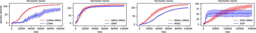
Figure 1: Learning curves in terms of episode rewards of COMA, MAAC, QMIX and DOP groups in randomly generated stochastic game.

4.5 Divergence-Regularized Actors

DAPO (Wang et al., 2019) analyzes the divergence-regularized MDP from the perspective of policy gradient theorem (Sutton et al., 2000) and gives an on-policy update rule for single-agent RL. Unlike existing work, we focus on a different perspective and derive an off-policy update rule by taking into consideration the characteristics of MARL.

From Lemma 2, we can obtain an optimization target for policy improvement,

$$\arg\min_{\bm{\pi}}D_{\operatorname{KL}}\bigg{(}{\bm{\pi}}(\cdot|s)\|{\bm{\rho}}(\cdot|s)\frac{\exp\left(Q^{{\bm{\pi}}_{\operatorname{old}}}_{\bm{\rho}}(s,\cdot)/\omega\right)}{Z^{\bm{\pi}_{\operatorname{old}}}(s)}\bigg{)}$$

$$\quad=\arg\max_{\bm{\pi}}\sum_{\bm{a}}{\bm{\pi}}(\bm{a}|s)\left(Q^{{\bm{\pi}}_{\operatorname{old}}}_{\bm{\rho}}(s,\bm{a})-\omega\log\frac{{\bm{\pi}}(\bm{a}|s)}{{\bm{\rho}}(\bm{a}|s)}\right).$$

Then, we can define the objective of the actors,

$$\mathcal{L}_{\bm{\pi}}=\mathbb{E}_{s\sim\mathcal{D}}\left[\sum_{\bm{a}}{\bm{\pi}}(\bm{a}|s)\left(Q^{{\bm{\pi}}_{\operatorname{old}}}_{\bm{\rho}}(s,\bm{a})-\omega\log\frac{{\bm{\pi}}(\bm{a}|s)}{{\bm{\rho}}(\bm{a}|s)}\right)\right],$$

where $\mathcal{D}$ is the replay buffer. Suppose each individual policy $\pi_{i}$ has a corresponding parameterization $\theta_{i}$. We can obtain the following policy gradient for each agent with some derivations given in Appendix A.9,

$$\begin{split}&\nabla_{\theta_{i}}\mathcal{L}_{\bm{\pi}}\\ &=\mathbb{E}\bigg{[}\nabla_{\theta_{i}}\log\pi_{i}(a_{i}|s)\Big{(}Q^{{\bm{\pi}}_{\operatorname{old}}}_{\bm{\rho}}(s,\bm{a})-\omega\log\frac{{\bm{\pi}}(\bm{a}|s)}{{\bm{\rho}}(\bm{a}|s)}-\omega\Big{)}\bigg{]}.\end{split}$$

We need to point out that the key to off-policy update is that Lemma 2 does not limit the state distribution. It only requires the condition is satisfied for each state. Therefore, we can maintain a replay buffer to cover different states as much as possible, which is a common practice in off-policy learning. DAPO uses a similar formula to ours, but it obtains the formula from policy gradient theorem, which requires the state distribution of the current policy.

Further, we can add a counterfactual baseline to the gradient. First, we have the following equation about the counterfactual baseline (Foerster et al., 2018),

$$\mathbb{E}_{s\sim\mathcal{D},\bm{a}\sim\bm{\pi}}\left[\nabla_{\theta_{i}}\log{\pi}_{i}(a_{i}|s)b(s,a_{-i})\right]=0,$$

where $a_{-i}$ denotes the joint action of all agents except agent $i$. Next, we take the baseline as

$$b(s,a_{-i})=\mathbb{E}_{a_{i}\sim\pi_{i}}[(Q^{{\bm{\pi}}_{\operatorname{old}}}_{\bm{\rho}}(s,\bm{a})-\omega\log\frac{{\bm{\pi}}(\bm{a}|s)}{{\bm{\rho}}(\bm{a}|s)}-\omega)].$$

Then, the gradient for each agent $i$ can be modified as follows,

$$\begin{split}\nabla_{\theta_{i}}\mathcal{L}_{\bm{\pi}}&=\mathbb{E}\bigg{[}\nabla_{\theta_{i}}\log\pi_{i}(a_{i}|s)(Q^{{\bm{\pi}}_{\operatorname{old}}}_{\bm{\rho}}(s,\bm{a})-\omega\log\frac{\pi_{i}(a_{i}|s)}{\rho_{i}(a_{i}|s)}\\ &-\mathbb{E}_{a_{i}\sim\pi_{i}}[Q^{{\bm{\pi}}_{\operatorname{old}}}_{\bm{\rho}}(s,\bm{a})]+\omega D_{\operatorname{KL}}(\pi_{i}(\cdot|s)\|\rho_{i}(\cdot|s)))\bigg{]}.\end{split}$$

In addition to variance reduction and credit assignment, this counterfactual baseline eliminates the policies of other agents from the gradient. This property makes it convenient to calculate the gradient and easy to select the target policy for each agent. Moreover, if the linear value decomposition condition is satisfied, we have the following gradient formula,

$$\nabla_{\theta_{i}}\mathcal{L}_{\bm{\pi}}=\mathbb{E}\bigg{[}\nabla_{\theta_{i}}\log\pi_{i}(a_{i}|s)\big{(}k_{i}(s)A^{{\pi^{i}_{\operatorname{old}}}}_{\bm{\rho}}(s,a_{i})\\ \qquad-\omega\log\frac{\pi_{i}(a_{i}|s)}{\rho_{i}(a_{i}|s)}+\omega D_{\operatorname{KL}}(\pi_{i}(\cdot|s)\|\rho_{i}(\cdot|s))\big{)}\bigg{]},$$

$$\text{where }A^{\pi^{i}_{\operatorname{old}}}_{\bm{\rho}}(s,a_{i})=Q^{\pi^{i}_{\operatorname{old}}}_{\bm{\rho}}(s,a_{i})-\mathbb{E}_{\tilde{a}_{i}\sim\pi_{i}}\left[Q^{\pi^{i}_{\operatorname{old}}}_{\bm{\rho}}(s,\tilde{a}_{i})\right].$$

4.6 Algorithm

Every iteration of (3) needs a converged policy. However, it is intractable to perform this update rule precisely in practice. Thus, we propose an alternative approximate method. For each agent, we update the policy $\pi_{i}$ and the target policy $\rho_{i}$ respectively as $\theta_{i}=\theta_{i}+\beta\nabla_{\theta_{i}}\mathcal{L}_{\bm{\pi}}$ and $\tilde{\theta}_{i}=(1-\tau)\tilde{\theta}_{i}+\tau\theta_{i}$, where $\beta$ is the learning rate, $\tilde{\theta}_{i}$ is the weights of $\rho_{i}$, and $\tau$ is the hyperparameter for soft update. Here we use one gradient step to replace the $\max$ operator in (3). From Theorem 2 and previous discussion, we know that optimizing $\mathcal{L}_{\bm{\pi}}$ can maximize $J_{\bm{\rho}}({\bm{\pi}})$, so we use $\nabla_{\theta_{i}}\mathcal{L}_{\bm{\pi}}$ in the gradient step for off-policy training instead of the gradient step directly optimizing $J_{\bm{\rho}}({\bm{\pi}})$ in (1).

Moreover, even if we take the target policies $\{\bm{\rho}^{k}\}$ as the moving average of the policies $\{\bm{\pi}^{k}\}$, the properties such as monotonic improvements, convergences of value functions and policies, and the bound of the biases, will be still conserved. The details of these results are included in Appendix A.10.

Now we have all the update rules of DMAC. The training of DMAC is a typical off-policy learning process, which is given in Appendix B for completeness.

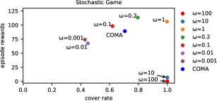
Figure 2: The scatter plot of the converged COMA and COMA+DMAC with different $\omega$ in terms of the episode rewards and cover rate in the randomly generated stochastic game.

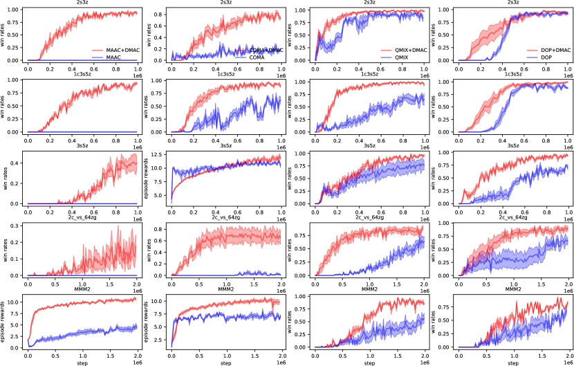
Figure 3: Learning curves in terms of win rates or episode rewards of COMA, MAAC, QMIX and DOP groups in five SMAC maps (each row corresponds to a map and each column corresponds to a group).

5 Experiments

In this section, we first empirically study the benefits of DMAC and investigate how DMAC improves the performance of existing MARL algorithms in a didactic stochastic game and five SMAC maps. Then, we demonstrate the advantages of divergence regularizer over entropy regularizer.

5.1 Improvements of Existing Methods

DMAC is a flexible framework and can be combined with many existing MARL algorithms. In the experiments, we choose four representative algorithms for different types of methods: COMA (Foerster et al., 2018) for on-policy multi-agent policy gradients, MAAC (Iqbal & Sha, 2019) for off-policy multi-agent actor-critic, QMIX (Rashid et al., 2018) for value decomposition, DOP (Wang et al., 2021b) for the combination of value decomposition and policy gradient. These algorithms need minor modifications to fit the framework of DMAC. We denote these modified algorithms as COMA+DMAC, MAAC+DMAC, QMIX+DMAC, and DOP+DMAC. Generally, our modification is limited and tries to keep the original architecture so as to fairly demonstrate the improvement of DMAC. The details of the modifications and hyperparameters are included in Appendix C. All the curves in our plots correspond to the mean value of five training runs with different random seeds, and shaded regions indicate 95% confidence interval.

A Didactic Example

We first test the four groups of methods in a stochastic game where agents share the reward. The stochastic game is generated randomly for the reward function and transition probabilities with 30 states, 3 agents and 5 actions for each agent. Each episode contains 30 timesteps in this game. The performance of these methods is illustrated in Figure 1. We can find that DMAC performs better than the baseline at the end of the training in all the four groups. Moreover, COMA+DMAC, QMIX+DMAC and MAAC+DMAC learn faster than their baselines. Though DOP learns faster than DOP+DMAC at the start, it falls into a sub-optimal policy and DOP+DMAC finds a better policy in the end.

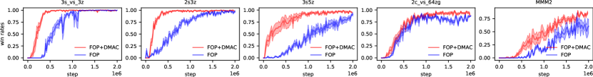
Figure 4: Learning curves in terms of win rates of FOP and FOP+DMAC in five SMAC maps.

We also show the benefit of exploration in this stochastic game for the convenience of statistics. We evaluate the exploration in terms of the cover rate of all state-action pairs, i.e., the ratio of the explored state-action pairs to all state-action pairs. The cover rates of COMA and COMA+DMAC with different $\omega$ are illustrated in Figure 2. We first study the effect of $\omega$ for the tradeoff between exploration and exploitation. From our previous analysis, a smaller $\omega$ gives a tighter bound for the converged performance of DMAC, but it also means that the benefits of the regularizer for exploration is smaller which will also affect the performance. So we need to choose a proper $\omega$ in practice. We can find in Figure 2 that when $\omega$ is large such as the case $\omega=10$ and $\omega=100$, the exploration is guaranteed but the performance is quite low since the regularizer is much larger than the environmental reward, and when $\omega$ is small such as the case $\omega=0.001$ and $\omega=0.01$, the performance is limited by the ability of exploration. Only when $\omega$ lies in a proper interval such as $\omega=0.1$, $\omega=0.2$ and $\omega=1$, the agents of DMAC can obtain a good balance between exploration and exploitation in this task.

We use COMA here as a representation of the traditional policy gradient method in cooperative MARL. In practice, we choose the $\omega=0.2$ for COMA+DMAC. We can find that the cover rate of COMA+DMAC ($\omega=0.2$) is higher than COMA, which can be an evidence for the benefit of exploration of DMAC. The cover rates of other three groups of algorithms and the learning curves for methods in Figure 2 are available in Appendix D.

SMAC

We test all the methods in five tasks of SMAC (Samvelyan et al., 2019). The introduction of the SMAC environment and the training details are included in Appendix C. The learning curves in terms of win rate (or episode rewards) of all the methods in the five SMAC maps are illustrated in Figure 3 (four columns for four groups of algorithms and five rows for five different maps in SMAC). For the case that both the baseline and DMAC can hardly win such as 3s5z and MMM2 for the COMA group and MMM2 for the MAAC group, we use the episode rewards to show the difference. In addition, the learning curves in terms of episode rewards are available in Appendix D, including two additional maps, 3m and 8m. We show the empirical result of DAPO in the map of 3m in the first figure of the second column in Figure 8 in Appendix D. It can be seen that DAPO cannot obtain a good performance in the simple task of SMAC, so we skip it in other SMAC tasks. The reason for the low performance of DAPO may be that DAPO omits the correction for $d_{\pi}(s)/d_{\pi_{t}}(s)$ in policy update which introduces bias in the gradient of policy, and uses V-trace as off-policy correction which however is biased. These drawbacks may be magnified in MARL settings. The superiority of our naturally off-policy method over the biased off-policy correction method can be partly seen from the large performance gap between COMA+DMAC and DAPO.

In all the five tasks, MAAC+DMAC outperforms MAAC significantly, but MAAC+DMAC does not change the network architecture of MAAC, which shows the benefits of divergence regularizer. As for the result of COMA and COMA+DMAC. We find that COMA+DMAC has higher win rates than COMA in most cases at the end of the training, which can be attributed to the benefits of off-policy learning and exploration of divergence regularizer. Though in some cases COMA learns faster than COMA+DMAC, it falls into sub-optimal in the end. This phenomenon can be observed more clearly in the plots of episode rewards in the hard tasks like 3s5z. This can be an evidence for the advantage of divergence regularizer which helps the agents find a better policy.

The stable policy improvement of divergence regularizer can be manifested by the small variance of the learning curves especially in the comparison between QMIX and QMIX+DMAC. In most tasks, we find that QMIX+DMAC learns substantially faster than QMIX and gets higher win rates in harder tasks. The results of DOP groups are illustrated in the fourth column of Figure 3. DOP+DMAC learns faster than DOP in most cases and finally obtains a better performance. The difference of DOP and DOP+DMAC can also partly show the advantage of naturally off-policy method to the off-policy correction method, as DOP+DMAC replaces the tree backup loss with off-policy TD($\lambda$).

DMAC improves the performance and/or convergence speed of the evaluated algorithms in most tasks. This empirically demonstrates the benefits of divergence regularizer. Moreover, the superiority of our naturally off-policy learning over the biased off-policy correction method can be partly witnessed from the empirical results.

5.2 Comparison with Entropy Regularization

FOP (Zhang et al., 2021) combines value decomposition with entropy regularization, which obtained the state-of-the-art performance in SMAC tasks. FOP has a well-tuned scheme for the temperature parameter of the entropy, so we take FOP as a strong baseline for entropy-regularized methods in cooperative MARL. We compare FOP and FOP+DMAC in five SMAC tasks, 3s_vs_3z, 2s3z, 3s5z, 2c_vs_64zg and MMM2, which respectively correspond to the three levels of difficulties (i.e., easy, hard, and super hard) for SMAC tasks. Three of these tasks are taken from the original paper of FOP. The modifications of FOP+DMAC are also included in Appendix C. The win rates of FOP and FOP+DMAC are illustrated in Figure 4. We can find that FOP+DMAC learns much faster than FOP in 3s_vs_3z, while it performs better than FOP in other four tasks. These results can be an evidence for the advantages of DMAC which could guarantee the monotonic improvement in the original MDP.

6 Conclusion

We propose a multi-agent actor-critic framework, DMAC, for cooperative MARL. We investigate divergence regularization, derive divergence policy iteration, and deduce the update rules for the critic, policy, and target policy in multi-agent settings. DMAC is a naturally off-policy framework and the divergence regularizer is beneficial to exploration and stable policy improvement. DMAC is also a flexible framework and can be combined with many existing MARL algorithms. It is empirically demonstrated that combining DMAC with existing MARL algorithms can improve the performance and convergence speed in a stochastic game and SMAC tasks.

Appendix A Proofs

A.1 Proposition 2

Proof.

For the sake of simplicity, we define $\tilde{Q}^{k}=Q^{*}_{\bm{\pi}^{k-1}}$ and $\tilde{V}^{k}=V^{*}_{\bm{\pi}^{k-1}}$. From the definition of iteration (3), we have $\bm{\pi}^{k}=\bm{\pi}^{*}_{\bm{\pi}^{k-1}}$. Then from Proposition 1, we also have $\tilde{Q}^{k}\to\tilde{Q}^{*}$ and $\tilde{V}^{k}\to\tilde{V}^{*}$.

From Proposition 5, we have $\bm{\pi}^{k}(\bm{a}|s)\propto\bm{\pi}^{k-1}(\bm{a}|s)\exp(\frac{\tilde{Q}^{k}(s,\bm{a})}{\omega})$. We define $f^{k}(s,\bm{a})=\exp(\frac{\tilde{Q}^{k}(s,\bm{a})}{\omega})$ and $f^{*}(s,\bm{a})=\exp(\frac{\tilde{Q}^{*}(s,\bm{a})}{\omega})$, then we have $f^{k}(s,\bm{a})\to f^{*}(s,\bm{a})$. Next we will show that $\bm{\pi}^{k}(\bm{a}|s)\propto\bm{\pi}^{0}(\bm{a}|s)\Pi_{i=1}^{k}f^{i}(s,\bm{a})$ or $\bm{\pi}^{k}(\bm{a}|s)=\frac{\bm{\pi}^{0}(\bm{a}|s)\Pi_{i=1}^{k}f^{i}(s,\bm{a})}{Z^{k}(s)}$ by induction, where $Z^{k}(s)=\sum_{\bm{a}^{\prime}}\bm{\pi}^{0}(\bm{a}^{\prime}|s)\Pi_{i=1}^{k}f^{i}(s,\bm{a}^{\prime})$ .

$$\bm{\pi}^{k}(\bm{a}|s) =\frac{\bm{\pi}^{k-1}(\bm{a}|s)f^{k}(s,\bm{a})}{\sum_{\bm{a}^{\prime}}\bm{\pi}^{k-1}(\bm{a}^{\prime}|s)f^{k}(s,\bm{a}^{\prime})}$$

$$=\frac{\frac{\bm{\pi}^{0}(\bm{a}|s)\Pi_{i=1}^{k-1}f^{i}(s,\bm{a})}{Z^{k-1}(s)}f^{k}(s,\bm{a})}{\sum_{\bm{a}^{\prime}}\frac{\bm{\pi}^{0}(\bm{a}^{\prime}|s)\Pi_{i=1}^{k-1}f^{i}(s,\bm{a}^{\prime})}{Z^{k-1}(s)}f^{k}(s,\bm{a}^{\prime})}\quad\text{(By induction)}$$

$$=\frac{\bm{\pi}^{0}(\bm{a}|s)\Pi_{i=1}^{k}f^{i}(s,\bm{a})}{\sum_{\bm{a}^{\prime}}\bm{\pi}^{0}(\bm{a}^{\prime}|s)\Pi_{i=1}^{k}f^{i}(s,\bm{a}^{\prime})}$$

$$=\frac{\bm{\pi}^{0}(\bm{a}|s)\Pi_{i=1}^{k}f^{i}(s,\bm{a})}{Z^{k}(s)}$$

We define $f^{*}_{s}=\max_{\bm{a}}f^{*}(s,\bm{a})$, then we will consider $\tilde{\pi}^{*}(\bm{a}|s)=\lim_{k\to\infty}\pi^{k}(\bm{a}|s)$.

$$\lim_{k\to\infty}\pi^{k}(\bm{a}|s) =\lim_{k\to\infty}\frac{\bm{\pi}^{0}(\bm{a}|s)\Pi_{i=1}^{k}f^{i}(s,\bm{a})}{\sum_{\bm{a}^{\prime}}\bm{\pi}^{0}(\bm{a}^{\prime}|s)\Pi_{i=1}^{k}f^{i}(s,\bm{a}^{\prime})}$$

$$=\lim_{k\to\infty}\frac{\bm{\pi}^{0}(\bm{a}|s)\frac{\Pi_{i=1}^{k}f^{i}(s,\bm{a})}{f^{*}(s,\bm{a})^{k}}\frac{f^{*}(s,\bm{a})^{k}}{(f^{*}_{s})^{k}}}{\sum_{\bm{a}^{\prime}}\bm{\pi}^{0}(\bm{a}^{\prime}|s)\frac{\Pi_{i=1}^{k}f^{i}(s,\bm{a}^{\prime})}{f^{*}(s,\bm{a}^{\prime})^{k}}\frac{f^{*}(s,\bm{a}^{\prime})^{k}}{(f^{*}_{s})^{k}}}$$

$$=\frac{\bm{\pi}^{0}(\bm{a}|s)\lim_{k\to\infty}\frac{\Pi_{i=1}^{k}f^{i}(s,\bm{a})}{f^{*}(s,\bm{a})^{k}}\frac{f^{*}(s,\bm{a})^{k}}{(f^{*}_{s})^{k}}}{\sum_{\bm{a}^{\prime}}\bm{\pi}^{0}(\bm{a}^{\prime}|s)\lim_{k\to\infty}\frac{\Pi_{i=1}^{k}f^{i}(s,\bm{a}^{\prime})}{f^{*}(s,\bm{a}^{\prime})^{k}}\frac{f^{*}(s,\bm{a^{\prime}})^{k}}{(f^{*}_{s})^{k}}}$$

$$=\mathbbm{1}{(\bm{a}\in U_{s})}\frac{\bm{\pi}^{0}(\bm{a}|s)}{\sum_{\bm{a}^{\prime}\in U_{s}}\bm{\pi}^{0}(\bm{a}^{\prime}|s)}$$

The last equation is actually from two simple conclusion: (1) If a sequence $\{a_{k}\}>0$ and $a_{k}\to A>0$, then $\lim_{n\to\infty}\frac{\Pi_{k=1}^{n}a_{k}}{A^{n}}=1$ ; (2) For $A>B>0$, $\lim_{n\to\infty}\frac{B^{n}}{A^{n}}=0$. So $\lim_{k\to\infty}\frac{\Pi_{i=1}^{k}f^{i}(s,\bm{a})}{f^{*}(s,\bm{a})^{k}}\frac{f^{*}(s,\bm{a})^{k}}{(f^{*}_{s})^{k}}=\mathbbm{1}{(\bm{a}\in U_{s})}$. ∎

A.2 Theorem 1

We define two operator $\Gamma$ and $\Gamma_{\omega}$ as

$$\Gamma V(s)=\max_{\bm{\pi}}\sum_{\bm{a}}\pi(\bm{a}|s)(r(s,\bm{a})+\gamma\mathbb{E}[V(s^{\prime})])$$

$$\Gamma_{\omega}V(s)=\max_{\bm{\pi}}\sum_{\bm{a}}\pi(\bm{a}|s)(r(s,\bm{a})+\gamma\mathbb{E}[V(s^{\prime})])-\omega D_{\operatorname{KL}}(\bm{\pi}(\cdot|s)||\tilde{\bm{\pi}}^{*}(\cdot|s))$$

From the result of traditional Q-learning (Sutton & Barto, 2018), we know that $\Gamma$ is a $\gamma$-contraction and the unique fixed point is the global optimal V-function $V^{*}$.

As for $\Gamma_{\omega}$, we have the following lemma from Yang et al. (2019):

Lemma 4.

• $\Gamma_{\omega}$ is a $\gamma$-contraction.

• If $V_{1}(s)\leq V_{2}(s)$ for all state $s$, then $\Gamma_{\omega}V_{1}(s)\leq\Gamma_{\omega}V_{2}(s)$ for all state $s$

• For any constant $c$, we define $(V+c)(s)=V(s)+c$, then $\Gamma_{\omega}(V+c)(s)=\Gamma_{\omega}V(s)+\gamma c$

Moreover, from the definition we know that $\tilde{V}^{k}(s)=\max_{\bm{\pi}}\sum_{\bm{a}}\pi(\bm{a}|s)(r(s,\bm{a})+\gamma\mathbb{E}[\tilde{V}^{k}(s^{\prime})])-\omega D_{\operatorname{KL}}(\bm{\pi}(\cdot|s)||{\bm{\pi}}^{k-1}(\cdot|s)$ and $\tilde{V}^{k}\to\tilde{V}^{*},\bm{\pi}^{k}\to\tilde{\bm{\pi}}^{*}$, then we have:

$$\tilde{V}^{*}(s)=\max_{\bm{\pi}}\sum_{\bm{a}}\pi(\bm{a}|s)(r(s,\bm{a})+\gamma\mathbb{E}[\tilde{V}^{*}(s^{\prime})])-\omega D_{\operatorname{KL}}(\bm{\pi}(\cdot|s)||\tilde{\bm{\pi}}^{*}(\cdot|s))$$

This means that $\tilde{V}^{*}$ is the unique fix point of $\Gamma_{\omega}$. Now we have all the tools for the proof of proposition 1. And this proof is inspired by Yang et al. (2019).

Proof.

Given that the initial policy is a uniform distribution, we know from Proposition 2 that:

$$\tilde{\bm{\pi}}^{*}(\bm{a}|s)=\mathbbm{1}(\bm{a}\in U_{s})\frac{1}{|U_{s}|},$$ (6)

where $|U_{s}|$ is the number of actions contained in the set $U_{s}$. Then we consider $D_{\operatorname{KL}}(\bm{\pi}(\cdot|s)||\tilde{\bm{\pi}}^{*}(\cdot|s))$ and have:

$$D_{\operatorname{KL}}(\bm{\pi}(\cdot|s)||\tilde{\bm{\pi}}^{*}(\cdot|s)) =\sum_{\bm{a}\in U_{s}}\bm{\pi}(\bm{a}|s)\log\frac{\bm{\pi}(\bm{a}|s)}{\tilde{\bm{\pi}}^{*}(\bm{a}|s)}$$ (7)

$$=\sum_{\bm{a}\in U_{s}}\bm{\pi}(\bm{a}|s)\log\bm{\pi}(\bm{a}|s)-\sum_{\bm{a}\in U_{s}}\bm{\pi}(\bm{a}|s)\log\tilde{\bm{\pi}}^{*}(\bm{a}|s)$$ (8)

$$\leq-\sum_{\bm{a}\in U_{s}}\bm{\pi}(\bm{a}|s)\log\tilde{\bm{\pi}}^{*}(\bm{a}|s)\quad(\bm{\pi}(\bm{a}|s)\leq 1)$$ (9)

$$=\log|U_{s}|\sum_{\bm{a}\in U_{s}}\bm{\pi}(\bm{a}|s)$$ (10)

$$\leq\log|U_{s}|\quad(\sum_{\bm{a}\in U_{s}}\bm{\pi}(\bm{a}|s)\leq\sum_{\bm{a}\in A}\bm{\pi}(\bm{a}|s)=1)$$ (11)

$$\leq\log|A|$$ (12)

Next we will consider the relation between $\Gamma_{\omega}$ and $\Gamma$:

$$\begin{split}\Gamma_{\omega}V(s)&=\max_{\bm{\pi}}\sum_{\bm{a}}\pi(\bm{a}|s)(r(s,\bm{a})+\gamma\mathbb{E}[V(s^{\prime})])-\omega D_{\operatorname{KL}}(\bm{\pi}(\cdot|s)||\tilde{\bm{\pi}}^{*}(\cdot|s))\\ &\leq\max_{\bm{\pi}}\sum_{\bm{a}}\pi(\bm{a}|s)(r(s,\bm{a})+\gamma\mathbb{E}[V(s^{\prime})])\\ &=\Gamma V(s)\end{split}$$ (13)

$$\begin{split}\Gamma_{\omega}V(s)&=\max_{\bm{\pi}}\sum_{\bm{a}}\pi(\bm{a}|s)(r(s,\bm{a})+\gamma\mathbb{E}[V(s^{\prime})])-\omega D_{\operatorname{KL}}(\bm{\pi}(\cdot|s)||\tilde{\bm{\pi}}^{*}(\cdot|s))\\ &\geq\max_{\bm{\pi}}\sum_{\bm{a}}\pi(\bm{a}|s)(r(s,\bm{a})+\gamma\mathbb{E}[V(s^{\prime})])-\max_{\bm{\pi}}D_{\operatorname{KL}}(\bm{\pi}(\cdot|s)||\tilde{\bm{\pi}}^{*}(\cdot|s))\\ &\geq\Gamma V(s)-\omega\log|A|\quad(\text{From the inequality \eqref{KL-bound}})\end{split}$$ (14)

We will show that $\Gamma^{k}V(s)-\omega\log|A|\sum_{t=0}^{k-1}\gamma^{t}\leq\Gamma_{\omega}^{k}V(s)\leq\Gamma^{k}V(s)$ for any $V$ and state $s$ by induction.

LHS:

$$\Gamma_{\omega}^{k+1}V(s) =\Gamma_{\omega}(\Gamma_{\omega}^{k}V(s))$$

$$\geq\Gamma_{\omega}(\Gamma^{k}V(s)-\omega\log|A|\sum_{t=0}^{k-1}\gamma^{t})\quad(\text{From the induction and the monotonicity in lemma \ref{reg-lemma}})$$

$$=\Gamma_{\omega}(\Gamma^{k}V(s))-\omega\log|A|\sum_{t=0}^{k-1}\gamma^{t+1}\quad(\text{From the conclusion about constant in lemma \ref{reg-lemma}})$$

$$\geq\Gamma^{k+1}V(s)-\omega\log|A|-\omega\log|A|\sum_{t=0}^{k-1}\gamma^{t+1}\quad(\text{From the inequality \ref{gamma-lower} })$$

$$=\Gamma^{k+1}V(s)-\omega\log|A|\sum_{t=0}^{k}\gamma^{t}$$

RHS:

$$\Gamma_{\omega}^{k+1}V(s) =\Gamma_{\omega}(\Gamma_{\omega}^{k}V(s))$$

$$\leq\Gamma_{\omega}(\Gamma^{k}V(s))\quad(\text{From the induction and the monotonicity in lemma \ref{reg-lemma}})$$

$$\leq\Gamma^{k+1}V(s)\quad(\text{From the inequality \ref{gamma-upper} })$$

Finally, with all these results above, let $k\to\infty$. As both $\Gamma_{\omega}$ and $\Gamma$ are $\gamma$-contraction, $\Gamma_{\omega}^{k}V\to\tilde{V}^{*},\Gamma^{k}V\to V^{*}$ for any $V$. We have:

$$\|\tilde{V}^{*}-V^{*}\|_{\infty}\leq\omega\log|A|\sum_{t=0}^{\infty}\gamma^{t}=\frac{\omega}{1-\gamma}\log|A|$$

∎

A.3 Lemma 1

Proof.

We define a new reward function

$$r_{\bm{\rho}}^{\bm{\pi}}(s,\bm{a})=r(s,\bm{a})-\omega\mathbb{E}_{s^{\prime}\sim P(\cdot|s,\bm{a})}\left[D_{\operatorname{KL}}\left({\bm{\pi}}(\cdot|s^{\prime})\|{\bm{\rho}}(\cdot|s^{\prime})\right)\right],$$

then we can rewrite the definition of operator $\Gamma^{\operatorname{\bm{\pi}}}_{\operatorname{\bm{\rho}}}$ as

$$\Gamma^{\operatorname{\bm{\pi}}}_{\operatorname{\bm{\rho}}}Q(s,\bm{a})=r_{\bm{\rho}}^{\bm{\pi}}(s,\bm{a})+\gamma\mathbb{E}_{s^{\prime}\sim P(\cdot|s,\bm{a}),\bm{a^{\prime}}\sim\bm{\pi}(\cdot|s^{\prime})}\left[Q(s^{\prime},\bm{a^{\prime}})\right].$$

With this formula, we can apply the traditional convergence result of policy evaluation in Sutton & Barto (2018). ∎

A.4 Lemma 2

For the proof of Lemma 2, we need the following lemma (Haarnoja et al., 2018) about improving policy in entropy-regularized MDP.

Lemma 5.

If we have a new policy ${\bm{\pi}}_{\operatorname{new}}$ and

$${\bm{\pi}}_{\operatorname{new}}=\arg\min_{\bm{\pi}}D_{\operatorname{KL}}\left({\bm{\pi}}(\cdot|s)\|\frac{\exp\left(Q^{{\bm{\pi}}_{\operatorname{{old}}}}_{\operatorname{ent}}(s,\cdot)/\omega\right)}{Z^{{\bm{\pi}}_{\operatorname{{old}}}}(s)}\right),$$

where $Z^{{\bm{\pi}}_{\operatorname{{old}}}}(s)$ represents the normalization term, then we have

$$Q^{{\bm{\pi}}_{\operatorname{{new}}}}_{\operatorname{ent}}(s,a)\geq Q^{{\bm{\pi}}_{\operatorname{{old}}}}_{\operatorname{ent}}(s,a),\quad\forall s\in S,a\in A.$$

With Lemma 5, we have the following proof of Lemma 2.

Proof.

Let $\hat{Q}$ be the same as the definition in Proof A.7. Then we have $\hat{Q}^{{\bm{\pi}}}(s,\bm{a})=Q^{{\bm{\pi}}}_{\bm{\rho}}(s,\bm{a})+\omega\log{\bm{\rho}}(\bm{a}|s),\,\forall{\bm{\pi}}$.

According to Lemma 5,

$$\hat{{\bm{\pi}}}_{\operatorname{{new}}}(s,\cdot)=\arg\min_{\bm{\pi}}D_{\operatorname{KL}}\left({\bm{\pi}}(\cdot|s)\|\frac{\exp\left(\hat{Q}^{{\bm{\pi}}_{\operatorname{{old}}}}(s,\cdot)/\omega\right)}{Z^{{\bm{\pi}}_{\operatorname{{old}}}}(s)}\right)$$

$$\hat{Q}^{\hat{{\bm{\pi}}}_{\operatorname{{new}}}}(s,\bm{a})\geq\hat{Q}^{{\bm{\pi}}_{\operatorname{{old}}}}(s,\bm{a}),\quad\forall\bm{a}\in A.$$

With the definition, we have

$$D_{\operatorname{KL}}\left({\bm{\pi}}(\cdot|s)\|\frac{\exp(\hat{Q}^{{\bm{\pi}}_{\operatorname{{old}}}}(s,\cdot)/\omega)}{Z^{{\bm{\pi}}_{\operatorname{{old}}}}(s)}\right)=D_{\operatorname{KL}}\left({\bm{\pi}}(\cdot|s)\|{\bm{\rho}}(\cdot|s)\frac{\exp(Q^{{\bm{\pi}}_{\operatorname{{old}}}}_{\bm{\rho}}(s,\cdot)/\omega)}{Z^{{\bm{\pi}}_{\operatorname{{old}}}}(s)}\right)$$

$${\bm{\pi}}_{\operatorname{{new}}}=\hat{{\bm{\pi}}}_{\operatorname{{new}}}$$

$$Q^{{\bm{\pi}}_{\operatorname{{new}}}}_{\bm{\rho}}(s,\bm{a})=\hat{Q}^{{\bm{\pi}}_{\operatorname{{new}}}}(s,\bm{a})-\omega\log{\bm{\rho}}(\bm{a}|s)\geq\hat{Q}^{{\bm{\pi}}_{\operatorname{{old}}}}(s,\bm{a})-\omega\log{\bm{\rho}}(\bm{a}|s)=Q^{{\bm{\pi}}_{\operatorname{old}}}_{\bm{\rho}}(s,\bm{a}).$$

∎

A.5 Lemma 3

Proof.

From the equation

$$\pi_{\operatorname{new}}^{i}=\arg\max_{\pi_{i}}\sum_{a_{i}}\pi_{i}(a_{i}|s)\left(k_{i}(s)Q_{\operatorname{\rho}}^{\pi^{i}_{\operatorname{old}}}(s,a_{i})-\omega\log\frac{\pi_{i}(a_{i}|s)}{\rho_{i}(a_{i}|s)}\right),$$

we can obtain

$$\begin{split}&\sum_{a_{i}}\pi_{\operatorname{new}}^{i}(a_{i}|s)\left(k_{i}(s)Q_{\operatorname{\rho}}^{\pi^{i}_{\operatorname{old}}}(s,a_{i})-\omega\log\frac{\pi_{\operatorname{new}}^{i}(a_{i}|s)}{\rho_{i}(a_{i}|s)}\right)\\ &\geq\sum_{a_{i}}\pi_{\operatorname{old}}^{i}(a_{i}|s)\left(k_{i}(s)Q_{\operatorname{\rho}}^{\pi^{i}_{\operatorname{old}}}(s,a_{i})-\omega\log\frac{\pi_{\operatorname{old}}^{i}(a_{i}|s)}{\rho_{i}(a_{i}|s)}\right).\\ \end{split}$$ (15)

By taking expectation on the both side of (15), we can obtain the followings.

$$\begin{split}&\sum_{a_{-i}}\tilde{\pi}_{-i}(a_{-i}|s)\sum_{a_{i}}\pi_{\operatorname{new}}^{i}(a_{i}|s)\left(k_{i}(s)Q_{\operatorname{\rho}}^{\pi^{i}_{\operatorname{old}}}(s,a_{i})-\omega\log\frac{\pi_{\operatorname{new}}^{i}(a_{i}|s)}{\rho_{i}(a_{i}|s)}\right)\\ &\geq\sum_{a_{-i}}\tilde{\pi}_{-i}(a_{-i}|s)\sum_{a_{i}}\pi_{\operatorname{old}}^{i}(a_{i}|s)\left(k_{i}(s)Q_{\operatorname{\rho}}^{\pi^{i}_{\operatorname{old}}}(s,a_{i})-\omega\log\frac{\pi_{\operatorname{old}}^{i}(a_{i}|s)}{\rho_{i}(a_{i}|s)}\right)\\ &\forall i\in I\quad\forall\tilde{\pi}_{-i}\\ \end{split}$$ (16)

Moreover, we can easily have the following derivation,

$$\begin{split}&\sum_{a_{i}}\pi^{i}_{\operatorname{new}}(a_{i}|s)\left(k_{i}(s)Q_{\operatorname{\rho}}^{\pi^{i}_{\operatorname{old}}}(s,a_{i})+b(s)-\omega\log\frac{\pi_{\operatorname{new}}^{i}(a_{i}|s)}{\rho_{i}(a_{i}|s)}\right)\\ &=\sum_{a_{-i}}u_{1}(a_{-i}|s)\sum_{a_{i}}\pi^{i}_{\operatorname{new}}(a_{i}|s)\left(k_{i}(s)Q_{\operatorname{\rho}}^{\pi^{i}_{\operatorname{old}}}(s,a_{i})+b(s)-\omega\log\frac{\pi_{\operatorname{new}}^{i}(a_{i}|s)}{\rho_{i}(a_{i}|s)}\right)\\ &=\sum_{a_{-i}}u_{2}(a_{-i}|s)\sum_{a_{i}}\pi^{i}_{\operatorname{new}}(a_{i}|s)\left(k_{i}(s)Q_{\operatorname{\rho}}^{\pi^{i}_{\operatorname{old}}}(s,a_{i})+b(s)-\omega\log\frac{\pi_{\operatorname{new}}^{i}(a_{i}|s)}{\rho_{i}(a_{i}|s)}\right)\\ &\forall u_{1},u_{2}.\end{split}$$ (17)

Then we have

$$\begin{split}&\mathbb{E}_{\bm{a}\sim\bm{\pi}_{\operatorname{new}}}\left[Q^{\bm{\pi}_{\operatorname{old}}}_{\bm{\rho}}(s,\bm{a})-\log\frac{{\bm{\pi}_{\operatorname{new}}}(\bm{a}|s)}{{\bm{\rho}}(\bm{a}|s)}\right]\\ &=\sum_{\bm{a}}\bm{\pi}_{\operatorname{new}}(\bm{a}|s)\sum_{i}\left(k_{i}(s)Q_{\operatorname{\rho}}^{\pi^{i}_{\operatorname{old}}}(s,a_{i})+b(s)-\omega\log\frac{\pi_{\operatorname{new}}^{i}(a_{i}|s)}{\rho_{i}(a_{i}|s)}\right)\\ &=\sum_{\bm{a}}\bm{\pi}_{\operatorname{new}}(\bm{a}|s)\sum_{i}\left(k_{i}(s)Q_{\operatorname{\rho}}^{\pi^{i}_{\operatorname{old}}}(s,a_{i})+b(s)-\omega\log\frac{\pi_{\operatorname{new}}^{i}(a_{i}|s)}{\rho_{i}(a_{i}|s)}\right)\\ &=\sum_{i}\sum_{a_{-i}}\pi^{-i}_{\operatorname{new}}(a_{-i}|s)\sum_{a_{i}}\pi^{i}_{\operatorname{new}}(a_{i}|s)\left(k_{i}(s)Q_{\operatorname{\rho}}^{\pi^{i}_{\operatorname{old}}}(s,a_{i})+b(s)-\omega\log\frac{\pi_{\operatorname{new}}^{i}(a_{i}|s)}{\rho_{i}(a_{i}|s)}\right)\\ &=\sum_{i}\sum_{a_{-i}}\pi^{-i}_{\operatorname{old}}(a_{-i}|s)\sum_{a_{i}}\pi^{i}_{\operatorname{new}}(a_{i}|s)\left(k_{i}(s)Q_{\operatorname{\rho}}^{\pi^{i}_{\operatorname{old}}}(s,a_{i})+b(s)-\omega\log\frac{\pi_{\operatorname{new}}^{i}(a_{i}|s)}{\rho_{i}(a_{i}|s)}\right)\\ &\geq\sum_{i}\sum_{a_{-i}}\pi^{-i}_{\operatorname{old}}(a_{-i}|s)\sum_{a_{i}}\pi^{i}_{\operatorname{old}}(a_{i}|s)\left(k_{i}(s)Q_{\operatorname{\rho}}^{\pi^{i}_{\operatorname{old}}}(s,a_{i})+b(s)-\omega\log\frac{\pi_{\operatorname{old}}^{i}(a_{i}|s)}{\rho_{i}(a_{i}|s)}\right)\\ &=V^{\bm{\pi}_{\operatorname{old}}}_{\bm{\rho}}(s)\end{split}$$ (18)

The fourth equation is from (17) and the fifth inequality is from (16).

By repeatedly applying (18) and the relation $Q^{\bm{\pi}_{\operatorname{old}}}_{\bm{\rho}}(s,\bm{a})=r(s,\bm{a})+\gamma\mathbb{E}_{s^{\prime}}\left[V^{\bm{\pi}_{\operatorname{old}}}_{\bm{\rho}}(s^{\prime})\right]$, we can complete the proof as followings.

$$\begin{split}Q^{\bm{\pi}_{\operatorname{old}}}_{\bm{\rho}}(s,\bm{a})&=r(s,\bm{a})+\gamma\mathbb{E}_{s^{\prime}}\left[V^{\bm{\pi}_{\operatorname{old}}}_{\bm{\rho}}(s^{\prime})\right]\\ &\leq r(s,\bm{a})+\gamma\mathbb{E}_{s^{\prime}}\left[\mathbb{E}_{\bm{a}^{\prime}\sim\bm{\pi}_{\operatorname{new}}}\left[Q^{\bm{\pi}_{\operatorname{old}}}_{\bm{\rho}}(s^{\prime},,\bm{a}^{\prime})-\log\frac{{\bm{\pi}_{\operatorname{new}}}(\bm{a}^{\prime}|s^{\prime})}{{\bm{\rho}}(\bm{a^{\prime}}|s^{\prime})}\right]\right]\\ &=r(s,\bm{a})+\gamma\mathbb{E}_{s^{\prime}}\left[\mathbb{E}_{\bm{a}^{\prime}\sim\bm{\pi}_{\operatorname{new}}}\left[r(s^{\prime},\bm{a}^{\prime})+\gamma\mathbb{E}_{s^{\prime\prime}}\left[V^{\bm{\pi}_{\operatorname{old}}}_{\bm{\rho}}(s^{\prime\prime})\right]-\log\frac{{\bm{\pi}_{\operatorname{new}}}(\bm{a}^{\prime}|s^{\prime})}{{\bm{\rho}}(\bm{a}^{\prime}|s^{\prime})}\right]\right]\\ &\cdots\\ &\leq Q^{\bm{\pi}_{\operatorname{new}}}_{\bm{\rho}}(s,\bm{a})\\ \end{split}$$

∎

A.6 Theorem 2

Proof.

First, we will show that Divergence Policy Iteration will monotonically improve the policy. From Lemma 2, we know that

$$V^{\bm{\pi}_{\operatorname{new}}}_{\bm{\rho}}(s) =\mathbb{E}_{\bm{a}\sim\bm{\pi}_{\operatorname{new}}(\cdot|s)}\left[Q^{\bm{\pi}_{\operatorname{new}}}_{\bm{\rho}}(s,\bm{a})-\omega\log\frac{{\bm{\pi}_{\operatorname{new}}}(\bm{a}|s)}{{\bm{\rho}}(\bm{a}|s)}\right]$$

$$\geq\mathbb{E}_{\bm{a}\sim\bm{\pi}_{\operatorname{new}}(\cdot|s)}\left[Q^{\bm{\pi}_{\operatorname{old}}}_{\bm{\rho}}(s,\bm{a})-\omega\log\frac{{\bm{\pi}_{\operatorname{new}}}(\bm{a}|s)}{{\bm{\rho}}(\bm{a}|s)}\right]$$

$$\geq\mathbb{E}_{\bm{a}\sim\bm{\pi}_{\operatorname{old}}(\cdot|s)}\left[Q^{\bm{\pi}_{\operatorname{old}}}_{\bm{\rho}}(s,\bm{a})-\omega\log\frac{{\bm{\pi}_{\operatorname{old}}}(\bm{a}|s)}{{\bm{\rho}}(\bm{a}|s)}\right]$$

$$=V^{\bm{\pi}_{\operatorname{old}}}_{\bm{\rho}}(s).$$

The first inequality is from the conclusion of Lemma 2 that

$$Q^{\bm{\pi}_{\operatorname{new}}}_{\bm{\rho}}(s,\bm{a})\geq Q^{\bm{\pi}_{\operatorname{old}}}_{\bm{\rho}}(s,\bm{a})\quad\forall\bm{a}\in A,$$

and the second inequality is from the definition of $\bm{\pi}_{\operatorname{new}}$ that

$${\bm{\pi}}_{\operatorname{new}}=\arg\min_{\bm{\pi}}D_{\operatorname{KL}}\left({\bm{\pi}}(\cdot|s)\|\frac{\exp\left(Q^{{\bm{\pi}}_{\operatorname{{old}}}}_{\bm{\rho}}(s,\cdot)/\omega\right)}{Z^{{\bm{\pi}}_{\operatorname{{old}}}}(s)}\right).$$

Here we have $V^{\bm{\pi}_{\operatorname{new}}}(s)\geq V^{\bm{\pi}_{\operatorname{old}}}(s),\,\forall s\in S$, and thus $J_{\bm{\rho}}(\bm{\pi}_{\operatorname{new}})\geq J_{\bm{\rho}}(\bm{\pi}_{\operatorname{old}})$. So, Divergence Policy Iteration will monotonically improve the policy.

Since the $Q^{\bm{\pi}}_{\bm{\rho}}$ is bounded above (the reward function is bounded), the sequence of Q-function $\left\{Q^{k}\right\}$ of Divergence Policy Iteration will converge and the corresponding policy sequence will also converge to some policy $\bm{\pi}_{\operatorname{conv}}$. We need to show $\bm{\pi}_{\operatorname{conv}}=\bm{\pi}^{*}_{\bm{\rho}}$.

$$V^{\bm{\pi}_{\operatorname{conv}}}_{\bm{\rho}}(s) =\mathbb{E}_{\bm{a}\sim\bm{\pi}_{\operatorname{conv}}(\cdot|s)}\left[Q^{\bm{\pi}_{\operatorname{conv}}}_{\bm{\rho}}(s,\bm{a})-\omega\log\frac{{\bm{\pi}_{\operatorname{conv}}}(\bm{a}|s)}{{\bm{\rho}}(\bm{a}|s)}\right]$$

$$\geq\mathbb{E}_{\bm{a}\sim\bm{\pi}(\cdot|s)}\left[Q^{\bm{\pi}_{\operatorname{conv}}}_{\bm{\rho}}(s,\bm{a})-\omega\log\frac{{\bm{\pi}}(\bm{a}|s)}{{\bm{\rho}}(\bm{a}|s)}\right]$$

$$\geq\mathbb{E}_{\bm{a}\sim\bm{\pi}(\cdot|s)}\bigg{[}r(s,\bm{a})+\gamma\mathbb{E}_{\bm{a^{\prime}}\sim\bm{\pi}(\cdot|s^{\prime})}\bigg{[}Q^{\bm{\pi}_{\operatorname{conv}}}_{\bm{\rho}}(s^{\prime},\bm{a}^{\prime})-\omega\log\frac{{\bm{\pi}}(\bm{a}^{\prime}|s^{\prime})}{{\bm{\rho}}(\bm{a}^{\prime}|s^{\prime})}\bigg{]}-\omega\log\frac{{\bm{\pi}}(\bm{a}|s)}{{\bm{\rho}}(\bm{a}|s)}\bigg{]}$$

$$\cdots$$

$$\geq V^{\bm{\pi}}_{\bm{\rho}}(s).$$

The first inequality is from the definition of $\bm{\pi}_{\operatorname{conv}}$ that

$${\bm{\pi}}_{\operatorname{conv}}=\arg\min_{\bm{\pi}}D_{\operatorname{KL}}\left({\bm{\pi}}(\cdot|s)\|\frac{\exp\left(Q^{{\bm{\pi}}_{\operatorname{{conv}}}}_{\bm{\rho}}(s,\cdot)/\omega\right)}{Z^{{\bm{\pi}}_{\operatorname{{conv}}}}(s)}\right)$$

and all the other inequalities are just iteratively using the first inequality and the relation of $Q^{\bm{\pi}}_{\bm{\rho}}$ and $V^{\bm{\pi}}_{\bm{\rho}}$. With iterations, we replace all the $\bm{\pi}_{\operatorname{conv}}$ with $\bm{\pi}$ in the expression of $V^{\bm{\pi}_{\operatorname{conv}}}_{\bm{\rho}}(s)$ and finally we get $V^{\bm{\pi}}_{\bm{\rho}}(s)$. Therefore, we have

$$V_{\bm{\rho}}^{\bm{\pi}_{\operatorname{conv}}}(s)\geq V_{\bm{\rho}}^{\bm{\pi}}(s)\quad\forall s\in S\quad\forall\bm{\pi}\in\Pi$$

$$J_{\bm{\rho}}(\bm{\pi}_{\operatorname{conv}})\geq J_{\bm{\rho}}(\bm{\pi})\quad\forall\bm{\pi}\in\Pi$$

$$\bm{\pi}_{\operatorname{conv}}=\bm{\pi}^{*}_{\bm{\rho}}.$$

∎

A.7 Proposition 5

We have the following proposition.

Proposition 5.

If ${\bm{\pi}}^{*}_{\bm{\rho}}=\arg\max_{\bm{\pi}}J_{\bm{\rho}}({\bm{\pi}})$, and $V_{\bm{\rho}}^{*}(s)=V_{\bm{\rho}}^{{\bm{\pi}}^{*}_{\bm{\rho}}}(s)$ and $Q_{\bm{\rho}}^{*}(s,\bm{a})=Q_{\bm{\rho}}^{{\bm{\pi}}^{*}_{\bm{\rho}}}(s,\bm{a})$ are respectively the corresponding Q-function and V-function of ${\bm{\pi}}^{*}_{\bm{\rho}}$, then they satisfy the following properties:

$${\bm{\pi}}^{*}_{\bm{\rho}}(\bm{a}|s)\propto{\bm{\rho}}(\bm{a}|s)\exp\left(\frac{r(s,\bm{a})+\gamma\mathbb{E}\left[V^{*}_{\bm{\rho}}(s^{\prime})\right]}{\omega}\right)$$ (19)

$$V^{*}_{\bm{\rho}}(s)=\omega\log\sum_{\bm{a}}{\bm{\rho}}(\bm{a}|s)\exp\left(\frac{r(s,\bm{a})+\gamma\mathbb{E}\left[V^{*}_{\bm{\rho}}(s^{\prime})\right]}{\omega}\right)$$ (20)

$$Q_{\bm{\rho}}^{*}(s,\bm{a})=r(s,\bm{a})+\gamma\omega\mathbb{E}\Big{[}V^{*}_{\bm{\rho}}(s^{\prime})\Big{]}.$$ (21)

Before the proof of Proposition 5, we need some results about the optimal Q-function $Q^{*}_{\operatorname{ent}}$, the optimal V-function $V^{*}_{\operatorname{ent}}$, and the optimal policy ${\bm{\pi}}^{*}_{\operatorname{ent}}$ in entropy-regularized MDP. We have the following lemma (Nachum et al., 2017).

Lemma 6.

$${\bm{\pi}}^{*}_{\operatorname{ent}}(s,a)\propto\exp\left(\left(r(s,a)+\gamma\mathbb{E}_{s^{\prime}\sim P(\cdot|s,a)}\left[V^{*}_{\operatorname{ent}}(s^{\prime})\right]\right)/\omega\right)$$

$$V^{*}_{\operatorname{ent}}(s)=\omega\log\sum_{a}\exp\left(\left(r(s,a)+\gamma\mathbb{E}_{s^{\prime}\sim P(\cdot|s,a)}\left[V^{*}_{\operatorname{ent}}(s^{\prime})\right]\right)/\omega\right)$$

$$Q^{*}_{\operatorname{ent}}(s,a)=r(s,a)+\gamma\omega\mathbb{E}_{s^{\prime}\sim P(\cdot|s,a)}\left[\log\sum_{a^{\prime}}\exp\left(Q^{*}_{\operatorname{ent}}(s^{\prime},a^{\prime})/\omega\right)\right]$$

With Lemma 6, we can complete the proof of Proposition 5.

Proof.

Let $\hat{r}(s,\bm{a})=r(s,\bm{a})+\omega\log{\bm{\rho}}(\bm{a}|s)$, we consider the objective function

$$\hat{J}({\bm{\pi}})=\mathbb{E}_{\bm{\pi}}\left[\sum_{t=0}\gamma^{t}\left(\hat{r}(s_{t},\bm{a}_{t})-\omega\log{\bm{\pi}}(\bm{a}_{t}|s_{t})\right)\right].$$

Let $\hat{{\bm{\pi}}}^{*}(\bm{a}|s)$,$\hat{V}^{*}(s)$ and $\hat{Q}^{*}(s,\bm{a})$ be the corresponding optimal policy, V-function and Q-function of $\hat{J}({\bm{\pi}})$. By definition we can obtain

$$\hat{{\bm{\pi}}}^{*}(\bm{a}|s)={\bm{\pi}}_{\bm{\rho}}^{*}(\bm{a}|s)$$

$$\hat{V}^{*}(s)=\mathbb{E}_{\ \bm{a}\sim\hat{{\bm{\pi}}}^{*}(\cdot|s),s^{\prime}\sim P(\cdot|s,a)}\left[\hat{r}(s,\bm{a})+\gamma\hat{V}^{*}(s^{\prime})-\omega\log\hat{{\bm{\pi}}}^{*}(\bm{a}|s)\right]$$

$$\qquad\ \ =\mathbb{E}_{\ \bm{a}\sim{\bm{\pi}}_{\bm{\rho}}^{*}(\cdot|s),s^{\prime}\sim P(\cdot|s,a)}\left[r(s,\bm{a})+\gamma\hat{V}^{*}(s^{\prime})-\omega\log\frac{{\bm{\pi}}_{\bm{\rho}}^{*}(\bm{a}|s)}{{\bm{\rho}}(\bm{a}|s)}\right]$$

$$\qquad\ \ =V^{*}_{\bm{\rho}}(s)$$

$$\hat{Q}^{*}(s,\bm{a})=\hat{r}(s,\bm{a})+\mathbb{E}_{s^{\prime}\sim P(\cdot|s,a)}\left[\hat{V}^{*}(s^{\prime})\right]$$

$$\qquad\quad\ \ =r(s,\bm{a})+\mathbb{E}_{s^{\prime}\sim P(\cdot|s,a)}\left[V_{\bm{\rho}}^{*}(s^{\prime})\right]+\omega\log{\bm{\rho}}(\bm{a}|s)$$

$$\qquad\quad\ \ =Q^{*}_{\bm{\rho}}(s,\bm{a})+\omega\log{\bm{\rho}}(\bm{a}|s).$$

According to Lemma 6, we have

$${\bm{\pi}}^{*}_{\bm{\rho}}(\bm{a}|s)=\hat{{\bm{\pi}}}^{*}(\bm{a}|s)\propto\exp\left(\left(\hat{r}(s,\bm{a})+\gamma\mathbb{E}_{s^{\prime}\sim P(\cdot|s,a)}\left[\hat{V}^{*}(s^{\prime})\right]\right)/\omega\right)$$

$$\qquad\quad\,\,\,\,={\bm{\rho}}(\bm{a}|s)\exp\left(\left(r(s,\bm{a})+\gamma\mathbb{E}_{s^{\prime}\sim P(\cdot|s,a)}\left[V^{*}_{\bm{\rho}}(s^{\prime})\right]\right)/\omega\right)$$

$$V^{*}_{\bm{\rho}}(s)=\hat{V}^{*}(s)$$

$$\qquad\,\,\,\,=\omega\log\sum_{\bm{a}}\exp\left(\left(\hat{r}(s,\bm{a})+\gamma\mathbb{E}_{s^{\prime}\sim P(\cdot|s,a)}\left[\hat{V}^{*}(s^{\prime})\right]\right)/\omega\right)$$

$$\qquad\,\,\,\,=\omega\log\sum_{\bm{a}}{\bm{\rho}}(\bm{a}|s)\exp\left(\left(r(s,\bm{a})+\gamma\mathbb{E}_{s^{\prime}\sim P(\cdot|s,a)}\left[V^{*}_{\bm{\rho}}(s^{\prime})\right]\right)/\omega\right)$$

$$Q_{\bm{\rho}}^{*}(s,\bm{a})=\hat{Q}^{*}(s,\bm{a})-\omega\log{\bm{\rho}}(\bm{a}|s)$$

$$\qquad\quad\,\,\,\,=\hat{r}(s,\bm{a})+\gamma\omega\mathbb{E}_{s^{\prime}\sim P(\cdot|s,a)}\left[\log\sum_{\bm{a^{\prime}}}\exp\left(\hat{Q}^{*}(s^{\prime},\bm{a}^{\prime})/\omega\right)\right]-\omega\log{\bm{\rho}}(\bm{a}|s)$$

$$\qquad\quad\,\,\,\,=r(s,\bm{a})+\gamma\omega\mathbb{E}_{s^{\prime}\sim P(\cdot|s,a)}\left[\log\sum_{\bm{a^{\prime}}}{\bm{\rho}}(\bm{a}|s)\exp\left(Q^{*}_{\bm{\rho}}(s^{\prime},\bm{a}^{\prime})/\omega\right)\right].$$

∎

A.8 Proposition 4

Proof.

From Proposition 5, we can obtain

$${\bm{\pi}}^{*}_{\bm{\rho}}(\bm{a}|s) =\frac{{\bm{\rho}}(\bm{a}|s)\exp\left(\left(r(s,\bm{a})+\gamma\mathbb{E}\left[V^{*}_{\bm{\rho}}(s^{\prime})\right]\right)/\omega\right)}{\sum_{\bm{b}}{\bm{\rho}}(\bm{b}|s)\exp\left(\left(r(s,\bm{b})+\gamma\mathbb{E}\left[V^{*}_{\bm{\rho}}(s^{\prime})\right]\right)/\omega\right)}$$

$$=\frac{{\bm{\rho}}(\bm{a}|s)\exp\left(Q^{*}_{\bm{\rho}}(s,\bm{a})/\omega\right)}{\exp\left(V^{*}_{\bm{\rho}}(s)/\omega\right)}$$

$$={\bm{\rho}}(\bm{a}|s)\exp\left(\left(Q^{*}_{\bm{\rho}}(s,\bm{a})-V^{*}_{\bm{\rho}}(s)\right)/\omega\right).$$ (22)

By rearranging the equation, we have

$$V^{*}_{\bm{\rho}}(s)=Q^{*}_{\bm{\rho}}(s,\bm{a})-\omega\log\frac{{\bm{\pi}^{*}_{\bm{\rho}}}(\bm{a}|s)}{{\bm{\rho}}(\bm{a}|s)},$$ (23)

which is tenable for all actions $\bm{a}\in A$. ∎

A.9 Derivation of Gradient

$$\begin{split}\nabla_{\theta_{i}}\mathcal{L}_{\bm{\pi}}&=\mathbb{E}_{s\sim\mathcal{D}}\left[\sum_{\bm{a}}\nabla_{\theta_{i}}{\bm{\pi}}(\bm{a}|s)\left(Q^{{\bm{\pi}_{\operatorname{old}}}}_{\bm{\rho}}(s,\bm{a})-\omega\log\frac{{\bm{\pi}}(\bm{a}|s)}{{\bm{\rho}}(\bm{a}|s)}\right)+{\bm{\pi}}(\bm{a}|s)\nabla_{\theta_{i}}(-\omega\log\frac{{\bm{\pi}}(\bm{a}|s)}{{\bm{\rho}}(\bm{a}|s)})\right]\\ &=\mathbb{E}_{s\sim\mathcal{D}}\left[\sum_{\bm{a}}{\bm{\pi}}(\bm{a}|s)\nabla_{\theta_{i}}\log\pi_{i}(a_{i}|s)\left(Q^{{\bm{\pi}_{\operatorname{old}}}}_{\bm{\rho}}(s,\bm{a})-\omega\log\frac{{\bm{\pi}}(\bm{a}|s)}{{\bm{\rho}}(\bm{a}|s)}\right)-\omega{\bm{\pi}}(\bm{a}|s)\nabla_{\theta_{i}}\log\pi_{i}(a_{i}|s)\right]\\ &=\mathbb{E}_{s\sim\mathcal{D},a\sim\bm{\pi}}\bigg{[}\nabla_{\theta_{i}}\log\pi_{i}(a_{i}|s)\bigg{(}Q^{{\bm{\pi}_{\operatorname{old}}}}_{\bm{\rho}}(s,\bm{a})-\omega\log\frac{{\bm{\pi}}(\bm{a}|s)}{{\bm{\rho}}(\bm{a}|s)}-\omega\bigg{)}\bigg{]}\\ \end{split}$$

A.10 Theoretical Results for the Moving Average Case.

In the case where we take the target policies $\{\bm{\rho}^{t}\}$ as the moving average of the policies $\{\bm{\pi}^{t}\}$, we will formulate the iterations as followings:

$$\bm{\rho^{t}}=(1-\tau)\bm{\rho^{t-1}}+\tau\bm{\pi^{t-1}}$$

$$\bm{\pi}^{t}=\arg\max_{{\bm{\pi}}}\sum_{s,\bm{a}}\mu_{\bm{\pi}}(s,\bm{a})r(s,\bm{a})-\omega D_{\operatorname{C}}\left(\mu_{\bm{\pi}}\|\mu_{{\bm{\rho}}^{t}}\right).$$

Then we have:

$$J(\bm{\pi}^{t+1}) \geq J(\bm{\pi}^{t+1})-\omega D_{\operatorname{C}}\left(\mu_{\bm{\pi}^{t+1}}\|\mu_{{\bm{\rho}}^{t+1}}\right)=J_{{\bm{\rho}}^{t+1}}(\bm{\pi}^{t+1})$$

$$\geq J(\bm{\pi}^{t})-\omega D_{\operatorname{C}}\left(\mu_{\bm{\pi}^{t}}\|\mu_{{\bm{\rho}}^{t+1}}\right)$$

$$\geq J(\bm{\pi}^{t})-(1-\tau)\omega D_{\operatorname{C}}\left(\mu_{\bm{\pi}^{t}}\|\mu_{{\bm{\rho}}^{t}}\right)$$

$$\geq J(\bm{\pi}^{t})-\omega D_{\operatorname{C}}\left(\mu_{\bm{\pi}^{t}}\|\mu_{{\bm{\rho}}^{t}}\right)=J_{{\bm{\rho}}^{t}}(\bm{\pi}^{t}).$$

The third inequality could be obtained as following:

$$D_{\operatorname{C}}\left(\mu_{\bm{\pi}^{t}}\|\mu_{{\bm{\rho}}^{t+1}}\right)=\sum_{s,\bm{a}}\mu_{\bm{\pi}}(s,\bm{a})\log\frac{{\bm{\pi}}^{t}(\bm{a}|s)}{{\bm{\rho}}^{t+1}(\bm{a}|s)}$$

$$=\sum_{s,\bm{a}}\mu_{\bm{\pi}}(s,\bm{a})\log\frac{{\bm{\pi}}^{t}(\bm{a}|s)}{\tau{\bm{\pi}}^{t}(\bm{a}|s)+(1-\tau){\bm{\rho}}^{t}(\bm{a}|s)}$$

$$\leq\sum_{s,\bm{a}}\mu_{\bm{\pi}}(s,\bm{a})\bigg{[}\log{\bm{\pi}}^{t}(\bm{a}|s)-\left(\tau\log{\bm{\pi}}^{t}(\bm{a}|s)+(1-\tau)\log{\bm{\rho}}^{t}(\bm{a}|s)\right)\bigg{]}\qquad\text{from the concavity of $\log(\cdot)$}$$

$$=(1-\tau)\sum_{s,\bm{a}}\mu_{\bm{\pi}}(s,\bm{a})\log\frac{{\bm{\pi}}^{t}(\bm{a}|s)}{{\bm{\rho}}^{t}(\bm{a}|s)}$$

$$=(1-\tau)D_{\operatorname{C}}\left(\mu_{\bm{\pi}^{t}}\|\mu_{{\bm{\rho}}^{t}}\right).$$

So the sequence $\{J_{{\bm{\rho}}^{t}}(\bm{\pi}^{t})\}$ is still bounded and improving monotonically and will converge. With this result, we have $\tilde{Q}^{k}=Q^{*}_{\bm{\rho}^{k}}$ and $\tilde{V}^{k}=V^{*}_{\bm{\rho}^{k}}$ will converge to $\tilde{Q}^{*}$ and $\tilde{V}^{*}$.

Next we will consider the convergence of the sequence $\{\bm{\rho}^{t}\}$ and $\{\bm{\pi}^{t}\}$. From Proposition 5, we have the formulation that

$$\bm{\pi}^{t}(\bm{a}|s)=\frac{\bm{\rho}^{t}(\bm{a}|s)f^{t}(s,\bm{a})}{\sum_{\bm{b}}\bm{\rho}^{t}(\bm{b}|s)f^{t}(s,\bm{b})}$$ (24)

where $f^{t}(s,\bm{a})=\exp(\frac{\tilde{Q}^{t}(s,\bm{a})}{\omega})$ and $f^{t}(s,\bm{a})\to f^{*}(s,\bm{a})=\exp(\frac{\tilde{Q}^{*}(s,\bm{a})}{\omega})$.

We define $Z^{t}(s)=\sum_{\bm{b}}\bm{\rho}^{t}(\bm{b}|s)f^{t}(s,\bm{b})$ and will show that $\{Z^{t}(s)\}$ will converge for each state $s$. Actually, we will show that $\{Z^{t}(s)\}$ monotonically improves and is bounded.

With $Z^{t}(s)$, we could rewrite the the relation between $\bm{\rho}^{t+1}$ and $\bm{\rho}^{t}$ as followings:

$$\bm{\rho}^{t+1}(\bm{a}|s)=\left(1-\tau+\tau\frac{f^{t}(s,\bm{a})}{Z^{t}(s)}\right)\bm{\rho}^{t}(\bm{a}|s).$$ (25)

Then we have:

$$Z^{t+1}(s)-Z^{t}(s)=\sum_{\bm{b}}\bm{\rho}^{t+1}(\bm{b}|s)f^{t+1}(s,\bm{b})-\sum_{\bm{b}}\bm{\rho}^{t}(\bm{b}|s)f^{t}(s,\bm{b})$$

$$\geq\sum_{\bm{b}}\bm{\rho}^{t+1}(\bm{b}|s)f^{t}(s,\bm{b})--\sum_{\bm{b}}\bm{\rho}^{t}(\bm{b}|s)f^{t}(s,\bm{b})\quad\text{($f^{t+1}(s,\bm{b})\geq f^{t}(s,\bm{b})$ from $\{\tilde{Q}^{t}\}$ improve monotonically.) }$$

$$=\tau\sum_{\bm{b}}\frac{f^{t}(s,\bm{b})-Z^{t}(s)}{Z^{t}(s)}\bm{\rho}^{t}(\bm{b}|s)f^{t}(s,\bm{b})\qquad\text{from iteration \eqref{eq:rho-iteration}}$$

$$=\tau\frac{\sum_{\bm{b}}\bm{\rho}^{t}(\bm{b}|s)f^{t}(s,\bm{b})^{2}-Z^{t}(s)^{2}}{Z^{t}(s)}$$

$$=\tau\frac{\operatorname{Var}_{\bm{b}\sim\bm{\rho}^{t}(\cdot|s)}\left[f^{t}(s,\bm{b})\right]}{Z^{t}(s)}$$

$$\geq 0.$$

Moreover, let $M^{*}=\max_{s,\bm{a}}f^{*}(s,\bm{a})$. When $t$ is sufficiently large we have $f^{t}(s,\bm{a})\leq f^{*}(s,\bm{a})+1\leq M^{*}+1$. So $Z^{t}(s)\leq M^{*}+1$ when $t$ is sufficiently large. With all the above discussions, we show that $Z^{t}(s)$ converge to $Z^{*}(s)$.

Next we will divide the actions into three classes according to the relation between $f^{*}(s,\bm{a})$ and $Z^{*}(s)$,given any fixed state $s$. Let $I^{+}_{s}=\{\bm{a}\in A|f^{*}(s,\bm{a})>Z^{*}(s)\}$, $I^{-}_{s}=\{\bm{a}\in A|f^{*}(s,\bm{a})<Z^{*}(s)\}$, and $I^{0}_{s}=\{\bm{a}\in A|f^{*}(s,\bm{a})=Z^{*}(s)\}$. We will show three properties about these sets:

• $\forall\bm{a}\in I^{-}_{s},\quad\bm{\rho}^{t}(\bm{a}|s)\to 0$.

• $I^{+}_{s}=\emptyset$.

• $\sum_{\bm{a}\in I^{0}_{s}}\rho^{t}(\bm{a}|s)\to 1$.

It is obvious that the property (3) is an corollary of property (1) and (2). So we will focus on property (1) and (2).

As for property (1), consider any action $\bm{a}\in I^{-}_{s}$. Let $\epsilon=\frac{Z^{*}(s)-f^{*}(s,\bm{a})}{4}>0$, when $t$ is sufficiently large, we have $f^{t}(s,\bm{a})<f^{*}(s,\bm{a})+\epsilon=Z^{*}(s)-3\epsilon$ and $Z^{t}(s)>Z^{*}(s)-\epsilon$. Then we have

$$\bm{\rho}^{t+1}(\bm{a}|s) =\left(1-\tau+\tau\frac{f^{t}(s,\bm{a})}{Z^{t}(s)}\right)\bm{\rho}^{t}(\bm{a}|s)$$

$$<\left(1-\tau+\tau\frac{Z^{*}(s)-3\epsilon}{Z^{*}(s)+\epsilon}\right)\bm{\rho}^{t}(\bm{a}|s)$$

$$=\left(1-\frac{4\epsilon\tau}{Z^{*}(s)+\epsilon}\right)\bm{\rho}^{t}(\bm{a}|s).$$

Since the constant $1-\frac{4\epsilon\tau}{Z^{*}(s)+\epsilon}<1$, we know that $\bm{\rho}^{t}(\bm{a}|s)\to 0$ for action $\bm{a}$.

As for property (2), suppose that $I^{+}_{s}\not=\emptyset$. Then, we could take some action $\bm{a}\in I^{+}_{s}$. Let $\epsilon=\frac{f^{*}(s,\bm{a})-Z^{*}(s)}{4}>0$, when $t$ is sufficiently large, we have $f^{t}(s,\bm{a})>f^{*}(s,\bm{a})-\epsilon$ and $Z^{t}(s)<Z^{*}(s)+\epsilon=f^{*}(s,\bm{a})-3\epsilon$. Then we have

$$\bm{\rho}^{t+1}(\bm{a}|s) =\left(1-\tau+\tau\frac{f^{t}(s,\bm{a})}{Z^{t}(s)}\right)\bm{\rho}^{t}(\bm{a}|s)$$

$$>\left(1-\tau+\tau\frac{f^{*}(s,\bm{a})-\epsilon}{f^{*}(s,\bm{a})-3\epsilon}\right)\bm{\rho}^{t}(\bm{a}|s)$$

$$=\left(1+\frac{2\epsilon\tau}{f^{*}(s,\bm{a})-3\epsilon}\right)\bm{\rho}^{t}(\bm{a}|s).$$

Since the constant $1+\frac{2\epsilon\tau}{f^{*}(s,\bm{a})-3\epsilon}>1$, we know that $\bm{\rho}^{t}(\bm{a}|s)\to\infty$ for action $\bm{a}$. But we know that $\bm{\rho}^{t}(\bm{a}|s)\leq 1$ which is a contradiction.

From these three properties we actually know that $Z^{*}(s)=\max_{\bm{a}}f^{*}(s,\bm{a})$. The proof is as followings: from property (2) we know that $f^{*}(s,\bm{a})\leq Z^{*}(s),\forall\bm{a}\in A$; suppose that $f^{*}(s,\bm{a})<Z^{*}(s),\forall\bm{a}\in A$, then from property (1) we know that $\sum_{\bm{a}}\bm{\rho}^{t}(\bm{a}|s)\to 0$ which contradicts to $\sum_{\bm{a}}\bm{\rho}^{t}(\bm{a}|s)=1$. This fact could also be written as $I^{0}_{s}=U_{s}$, where $U_{s}$ is the same definition as the proof for Proposition 2 in Appendix A.1

Finally, with all these preparations above, we could discuss the convergence of $\bm{\pi}^{t}$.

From iteration (25), we could obtain the following formula:

$$\bm{\rho}^{t}(\bm{a}|s)=\bm{\rho}^{0}(\bm{a}|s)f^{t}(s,\bm{a})\Pi_{k=0}^{t}\left(1-\tau+\tau\frac{f^{k}(s,\bm{a})}{Z^{k}(s)}\right)=\bm{\pi}^{0}(\bm{a}|s)f^{t}(s,\bm{a})\Pi_{k=0}^{t}\left(1-\tau+\tau\frac{f^{k}(s,\bm{a})}{Z^{k}(s)}\right).$$ (26)

Combining this with (24), we have

$$\bm{\pi}^{t}(\bm{a}|s) =\frac{\bm{\pi}^{0}(\bm{a}|s)f^{t}(s,\bm{a})\Pi_{k=0}^{t-1}\left(1-\tau+\tau\frac{f^{k}(s,\bm{a})}{Z^{k}(s)}\right)}{\sum_{\bm{b}}\bm{\pi}^{0}(\bm{b}|s)f^{t}(s,\bm{b})\Pi_{k=0}^{t-1}\left(1-\tau+\tau\frac{f^{k}(s,\bm{b})}{Z^{k}(s)}\right)}$$

$$=\frac{\bm{\pi}^{0}(\bm{a}|s)f^{t}(s,\bm{a})\Pi_{k=0}^{t-1}\left((1-\tau)Z^{k}(s)+\tau f^{k}(s,\bm{a})\right)}{\sum_{\bm{b}}\bm{\pi}^{0}(\bm{b}|s)f^{t}(s,\bm{b})\Pi_{k=0}^{t-1}\left((1-\tau)Z^{k}(s)+\tau f^{k}(s,\bm{b})\right)}$$

$$=\frac{\bm{\pi}^{0}(\bm{a}|s)\frac{f^{t}(s,\bm{a})\Pi_{k=0}^{t-1}\left((1-\tau)Z^{k}(s)+\tau f^{k}(s,\bm{a})\right)}{\left(Z^{*}(s)\right)^{t+1}}}{\sum_{\bm{b}}\bm{\pi}^{0}(\bm{b}|s)\frac{f^{t}(s,\bm{b})\Pi_{k=0}^{t-1}\left((1-\tau)Z^{k}(s)+\tau f^{k}(s,\bm{b})\right)}{\left(Z^{*}(s)\right)^{t+1}}}.$$

We also have

$$\lim_{t\to\infty}\left((1-\tau)Z^{t}(s)+\tau f^{t}(s,\bm{a})\right)=\begin{cases}Z^{*}(s)&\bm{a}\in I^{0}_{s}\\ (1-\tau)Z^{*}(s)+\tau f^{*}(s,\bm{a})<Z^{*}(s)&\bm{a}\in I^{-}_{s}\end{cases}.$$ (27)

Similarly to the proof for Proposition 2, we have

$$\lim_{t\to\infty}\frac{f^{t}(s,\bm{a})\Pi_{k=0}^{t-1}\left((1-\tau)Z^{k}(s)+\tau f^{k}(s,\bm{a})\right)}{\left(Z^{*}(s)\right)^{t+1}}=\begin{cases}1&\bm{a}\in I^{0}_{s}\\ 0&\bm{a}\in I^{-}_{s}\end{cases}.$$ (28)

Finally we obtain

$$\tilde{\bm{\pi}}^{*}(\bm{a}|s)=\lim_{t\to\infty}\bm{\pi}^{t}(\bm{a}|s)=\mathbbm{1}{(\bm{a}\in I^{0}_{s})}\frac{\bm{\pi}^{0}(\bm{a}|s)}{\sum_{\bm{b}\in I^{0}_{s}}\bm{\pi}^{0}(\bm{b}|s)}=\mathbbm{1}{(\bm{a}\in U_{s})}\frac{\bm{\pi}^{0}(\bm{a}|s)}{\sum_{\bm{b}\in U_{s}}\bm{\pi}^{0}(\bm{b}|s)}.$$ (29)

This conclusion is actually the same as Proposition 2.

Moreover, as $\bm{\rho}^{t}$ is the moving average of $\bm{\pi}^{t}$, it is obvious that $\bm{\rho}^{t}\to\tilde{\bm{\pi}}^{*}$. With this result, we could define the same operator $\Gamma_{\omega}$ as the proof for Theorem 1 in Appendix A.2 and use the same proof to show that $\tilde{V}^{*}$ is the fixed point of $\Gamma_{\omega}$ and finally obtain the same conclusion of Theorem 1.

Appendix B Algorithm

Algorithm 1 gives the training procedure of DMAC.

Algorithm 1 DMAC

1:  for episode = $1$ to $m$ do

2:     Initialize the environment and receive initial state $s$  

3:     for $t=1$ to max-episode-length do

4:        For each agent $i$, select action $a_{i}\sim\pi_{i}(\cdot|s)$  

5:        Execute joint-action $\bm{a}=(a_{1},a_{2},\cdots,a_{n})$ and observe reward $r$ and next state $s^{\prime}$ 

6:        Store $(s,\bm{a},r,s^{\prime})$ in replay buffer $\mathcal{D}$  

7:     end for

8:     Sample a random minibatch of $K$ samples from $\mathcal{D}$, $\{(s_{k},\bm{a}_{k},r_{k},s^{\prime}_{k})\}_{K}$  

9:     for agent $i=1$ to $n$ do

10:        Update policy $\pi_{i}$: $\theta_{i}=\theta_{i}+\beta\nabla_{\theta_{i}}\mathcal{L}_{\bm{\pi}}$  

11:        Update target policy $\rho_{i}$: $\tilde{\theta}_{i}=(1-\tau)\tilde{\theta}_{i}+\tau\theta_{i}$  

12:     end for

13:     Update critic: $\phi=\phi-\alpha\nabla_{\phi}\mathcal{L}_{Q}$ 

14:     Update target critic: $\tilde{\phi}=(1-\tau)\tilde{\phi}+\tau\phi$  

15:  end for

Appendix C Implementation Details

SMAC is an MARL environment based on the game StarCraft II (SC2). Agents control different units in SC2 and can attack, move or take other actions. The general mode of SMAC tasks is that agents control a team of units to counter another team controlled by built-in AI. The target of agents is to wipe out all the enemy units and agents will gain rewards when hurting or killing enemy units. Agents have an observation range and can only observe information of units in this range, but the information of all the units can be accessed in training. We test all the methods in totally 8 tasks/maps: 3m, 2s3z, 3s5z, 8m, 1c3s5z, 3s_vs_3z, 2c_vs_64zg, and MMM2.

C.1 Modifications of the Baseline Methods

The modifications of the baseline methods, COMA, MAAC, QMIX, DOP, and FOP, are as follows:

• COMA. We keep the original critic and actor networks and add a target policy network with the same architecture as the actor. As COMA is on-policy but COMA+DMAC is off-policy, we add a replay buffer for experience replay.

• MAAC already has a target policy for stability, so we do not need to modify the network architecture. We only change the update rule for the critic and actors.

• QMIX is a value-based method, so we need to add a policy network and a target policy network for each agent. We keep the original individual Q-functions to learn the critic in QMIX+DMAC. In divergence-regularized MDP, the $\max$ operator is not needed in the critic update, so we abandon the hypernet and use an MLP, which takes individual Q-values and state as input and produces the joint Q-value. This architecture is simple and its expressive capability is not limited by QMIX’s IGM condition.

• DOP. We keep the original critic and actor networks and add a target policy network with the same architecture as the actor. We keep the value decomposition structure and use off-policy TD($\lambda$) for all samples in training to replace the tree backup loss and on-policy TD($\lambda$) loss.

• FOP. We replace the entropy regularizers with divergence regularizers in FOP and use the update rules of DMAC. We keep the original architecture of FOP.

C.2 Hyperparameters

As all tasks in our experiments are cooperative with shared reward, so we use parameter-sharing policy network and critic network for MAAC and MAAC+DMAC to accelerate training. Besides, we add a RNN layer to the policy network and critic network in MAAC and MAAC+DMAC to settle the partial observability.

All the policy networks are the same as two linear layers and one GRUCell layer with ReLU activation and the number of hidden units is 64. The individual Q-networks for QMIX group is the same as the policy network mentioned before. The critic network for COMA group is a MLP with three 128-unit hidden layers and ReLU activation. The attention dimension in the critic networks of MAAC group is 32. The number of hidden units of mixer network in QMIX group is 32. The learning rate for critic is $10^{-3}$ and the learning rate for actor is $10^{-4}$. We train all networks with RMSprop optimizer. The discouted factor is $\gamma=0.99$. The coefficient of regularizer is $\omega=0.01$ for SMAC tasks and $\omega=0.2$ for the stochastic game. The td_lambda factor used in COMA group is $0.8$. The parameter used for soft updating target policy is $\tau=0.01$. Our code is based on the implementation of PyMARL (Samvelyan et al., 2019), MAAC (Iqbal & Sha, 2019), DOP (Wang et al., 2021b), FOP (Zhang et al., 2021) and an open source code for algorithms in SMAC (https://github.com/starry-sky6688/StarCraft).

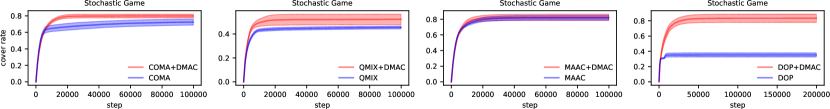
Figure 5: Learning curves in terms of cover rates of COMA, MAAC, QMIX and DOP groups in the randomly generated stochastic game.

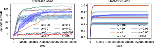
Figure 6: Learning curves in terms of cover rates of COMA and COMA+DMAC with different $\omega$ in the randomly generated stochastic game.

C.3 Experiment Settings

We trained each algorithms for five runs with different random seeds. In SMAC tasks, we train each algorithm for one million steps in each run for COMA, QMIX, MAAC, and DOP groups (except 2c_vs_64zg and MMM2) and two million steps for FOP groups. We evaluate 20 episodes in every 10000 training steps in the one million steps training procedure and in every 20000 steps in the two million steps training procedure. In evaluation, we select greedy actions for QMIX and FOP (following the setting in the FOP paper) and sample actions according to action distribution for stochastic policy (COMA, MAAC, DOP and divergence-regularized methods). We do all the experiments by a server with 2 NVIDIA A100 GPUs.

Appendix D Additional Results

Figure 5 shows the learning curves in terms of cover rates of COMA, QMIX, MAAC and DOP groups in the randomly generated stochastic game.

Figure 6 shows learning curves in terms of cover rates and episode rewards of COMA and COMA+DMAC with different $\omega$ in the randomly generated stochastic game.

Figure 7 and Figure 8 shows the learning curves of COMA, MAAC, QMIX and DOP groups in terms of mean episode rewards and win rates in seven SMAC maps.

Figure 9 shows the learning curves of FOP+DMAC and FOP in terms of mean episode rewards in 3s_vs_3z,2s3z,3s5z, 2c_vs_64zg and MMM2.

Figure 10 shows the learning curves in terms of mean episode rewards of COMA and DOP groups in the CDM environment used by the DOP paper.

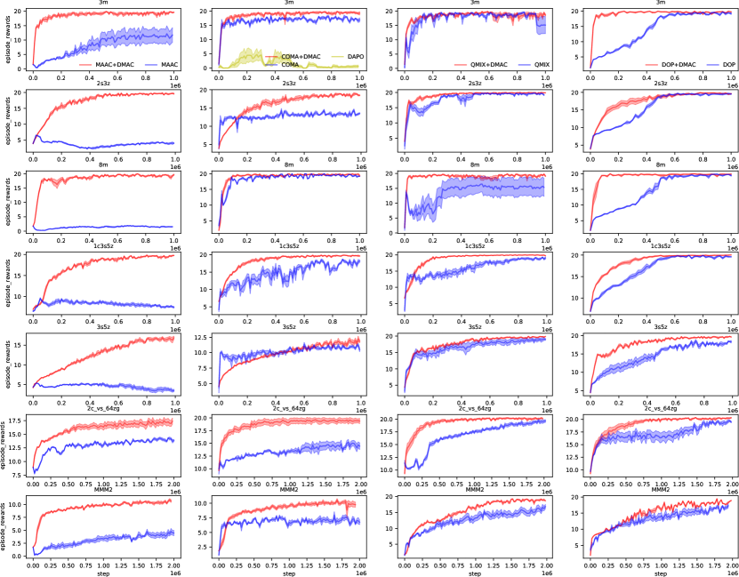
Figure 7: Learning curves in terms of mean episode reward of COMA, MAAC, QMIX, and DOP groups in seven SMAC maps (each row corresponds to a map and each column corresponds to a group).

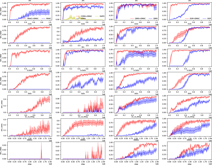
Figure 8: Learning curves in terms of win rate of COMA, MAAC, QMIX, and DOP groups in seven SMAC maps (each row corresponds to a map and each column corresponds to a group).

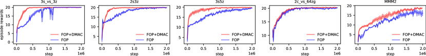
Figure 9: Learning curves in terms of mean episode rewards of FOP+DMAC and FOP in five SMAC maps (each column corresponds to a map).

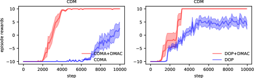
Figure 10: Learning curves in terms of mean episode rewards of COMA and DOP groups in the CDM environment used by the DOP paper.

References

• Agarwal et al. (2020) Agarwal, A., Kumar, S., Sycara, K., and Lewis, M. Learning Transferable Cooperative Behavior in Multi-Agent Team. In International Conference on Autonomous Agents and Multiagent Systems (AAMAS), 2020.
• Espeholt et al. (2018) Espeholt, L., Soyer, H., Munos, R., Simonyan, K., Mnih, V., Ward, T., Doron, Y., Firoiu, V., Harley, T., Dunning, I., et al. Impala: Scalable Distributed Deep-Rl with Importance Weighted Actor-Learner Architectures. In International Conference on Machine Learning (ICML), 2018.
• Eysenbach & Levine (2019) Eysenbach, B. and Levine, S. If MaxEnt RL Is The Answer, What Is The Question? arXiv preprint arXiv:1910.01913, 2019.
• Foerster et al. (2018) Foerster, J. N., Farquhar, G., Afouras, T., Nardelli, N., and Whiteson, S. Counterfactual Multi-Agent Policy Gradients. In AAAI Conference on Artificial Intelligence (AAAI), 2018.
• Grau-Moya et al. (2019) Grau-Moya, J., Leibfried, F., and Vrancx, P. Soft Q-Learning with Mutual-Information Regularization. In International Conference on Learning Representations (ICLR), 2019.
• Haarnoja et al. (2017) Haarnoja, T., Tang, H., Abbeel, P., and Levine, S. Reinforcement Learning with Deep Energy-Based Policies. In International Conference on Machine Learning (ICML), 2017.
• Haarnoja et al. (2018) Haarnoja, T., Zhou, A., Abbeel, P., and Levine, S. Soft Actor-Critic: Off-Policy Maximum Entropy Deep Reinforcement Learning with A Stochastic Actor. In International Conference on Machine Learning (ICML), 2018.
• Iqbal & Sha (2019) Iqbal, S. and Sha, F. Actor-Attention-Critic for Multi-Agent Reinforcement Learning. In International Conference on Machine Learning (ICML), 2019.
• Jiang et al. (2020) Jiang, J., Dun, C., Huang, T., and Lu, Z. Graph Convolutional Reinforcement Learning. In International Conference on Learning Representations (ICLR), 2020.
• Kakade & Langford (2002) Kakade, S. and Langford, J. Approximately Optimal Approximate Reinforcement Learning. In International Conference on Machine Learning (ICML), 2002.
• Lowe et al. (2017) Lowe, R., Wu, Y. I., Tamar, A., Harb, J., Abbeel, O. P., and Mordatch, I. Multi-Agent Actor-Critic for Mixed Cooperative-Competitive Environments. In Advances in Neural Information Processing Systems (NeurIPS), 2017.
• Nachum et al. (2017) Nachum, O., Norouzi, M., Xu, K., and Schuurmans, D. Bridging The Gap Between Value and Policy Based Reinforcement Learning. In Advances in Neural Information Processing Systems (NeurIPS), 2017.
• Nachum et al. (2018) Nachum, O., Norouzi, M., Xu, K., and Schuurmans, D. Trust-Pcl: An Off-Policy Trust Region Method for Continuous Control. In International Conference on Learning Representations (ICLR), 2018.
• Neu et al. (2017) Neu, G., Jonsson, A., and Gómez, V. A Unified View of Entropy-Regularized Markov Decision Processes. arXiv preprint arXiv:1705.07798, 2017.
• Oliehoek et al. (2016) Oliehoek, F. A., Amato, C., et al. A Concise Introduction To Decentralized POMDPs, volume 1. Springer, 2016.
• Pan et al. (2021) Pan, L., Rashid, T., Peng, B., Huang, L., and Whiteson, S. Regularized Softmax Deep Multi-Agent Q-Learning. Advances in Neural Information Processing Systems (NeurIPS), 2021.
• Peng et al. (2021) Peng, B., Rashid, T., de Witt, C. A. S., Kamienny, P.-A., Torr, P. H., Böhmer, W., and Whiteson, S. FACMAC: Factored Multi-Agent Centralised Policy Gradients. In Advances in Neural Information Processing Systems (NeurIPS), 2021.
• Rashid et al. (2018) Rashid, T., Samvelyan, M., De Witt, C. S., Farquhar, G., Foerster, J., and Whiteson, S. QMIX: Monotonic Value Function Factorisation for Deep Multi-Agent Reinforcement Learning. In International Conference on Machine Learning (ICML), 2018.
• Samvelyan et al. (2019) Samvelyan, M., Rashid, T., de Witt, C. S., Farquhar, G., Nardelli, N., Rudner, T. G., Hung, C.-M., Torr, P. H., Foerster, J. N., and Whiteson, S. The StarCraft Multi-Agent Challenge. In AAMAS, 2019.
• Schulman et al. (2015) Schulman, J., Levine, S., Abbeel, P., Jordan, M., and Moritz, P. Trust Region Policy Optimization. In International Conference on Machine Learning (ICML), 2015.
• Schulman et al. (2017) Schulman, J., Wolski, F., Dhariwal, P., Radford, A., and Klimov, O. Proximal Policy Optimization Algorithms. arXiv preprint arXiv:1707.06347, 2017.
• Son et al. (2019) Son, K., Kim, D., Kang, W. J., Hostallero, D. E., and Yi, Y. QTRAN: Learning To Factorize with Transformation for Cooperative Multi-Agent Reinforcement Learning. In International Conference on Machine Learning (ICML), 2019.
• Sun et al. (2021) Sun, W.-F., Lee, C.-K., and Lee, C.-Y. DFAC Framework: Factorizing The Value Function Via Quantile Mixture for Multi-Agent Distributional Q-Learning. In International Conference on Machine Learning (ICML), 2021.
• Sunehag et al. (2018) Sunehag, P., Lever, G., Gruslys, A., Czarnecki, W. M., Zambaldi, V. F., Jaderberg, M., Lanctot, M., Sonnerat, N., Leibo, J. Z., Tuyls, K., et al. Value-Decomposition Networks For Cooperative Multi-Agent Learning Based On Team Reward. In International Conference on Autonomous Agents and MultiAgent Systems (AAMAS), 2018.
• Sutton & Barto (2018) Sutton, R. S. and Barto, A. G. Reinforcement Learning: An Introduction. MIT press, 2018.
• Sutton et al. (2000) Sutton, R. S., McAllester, D. A., Singh, S. P., and Mansour, Y. Policy Gradient Methods for Reinforcement Learning with Function Approximation. In Advances in Neural Information Processing Systems (NeurIPS), 2000.
• Touati et al. (2020) Touati, A., Zhang, A., Pineau, J., and Vincent, P. Stable Policy Optimization Via Off-Policy Divergence Regularization. In Conference on Uncertainty in Artificial Intelligence (UAI), 2020.
• Wang et al. (2021a) Wang, J., Ren, Z., Liu, T., Yu, Y., and Zhang, C. QPLEX: Duplex Dueling Multi-Agent Q-Learning. In International Conference on Learning Representations (ICLR), 2021a.
• Wang et al. (2019) Wang, Q., Li, Y., Xiong, J., and Zhang, T. Divergence-Augmented Policy Optimization. In Advances in Neural Information Processing Systems (NeurIPS), 2019.
• Wang et al. (2021b) Wang, Y., Han, B., Wang, T., Dong, H., and Zhang, C. DOP: Off-Policy Multi-Agent Decomposed Policy Gradients. In International Conference on Learning Representations (ICLR), 2021b.
• Yang et al. (2019) Yang, W., Li, X., and Zhang, Z. A Regularized Approach To Sparse Optimal Policy in Reinforcement Learning. In Advances in Neural Information Processing Systems (NeurIPS), 2019.
• Yang et al. (2020) Yang, Y., Hao, J., Liao, B., Shao, K., Chen, G., Liu, W., and Tang, H. Qatten: A General Framework for Cooperative Multiagent Reinforcement Learning. arXiv preprint arXiv:2002.03939, 2020.
• Yu et al. (2021) Yu, C., Velu, A., Vinitsky, E., Wang, Y., Bayen, A. M., and Wu, Y. The Surprising Effectiveness of PPO in Cooperative, Multi-Agent Games. arXiv preprint arXiv:2103.01955, 2021.
• Zhang et al. (2021) Zhang, T., Li, Y., Wang, C., Xie, G., and Lu, Z. FOP: Factorizing Optimal Joint Policy of Maximum-Entropy Multi-Agent Reinforcement Learning. In International Conference on Machine Learning (ICML), 2021.