Timelike Transition Form Factor for
CP-odd Higgs Boson Production

15th International Symposium on Radiative Corrections:
Applications of Quantum Field Theory to Phenomenology,
FSU, Tallahasse, FL, USA, 17-21 May 2021 10.21468/SciPostPhysProc.?

Abstract

We investigate the production of CP-odd Higgs boson $A^{0}$ associated with a real $\gamma$ in $e^{+}e^{-}$ collisions. Because of the properties of $A^{0}$ coupling to the other fields, the main contribution comes from the top-quark triangle loop diagrams. We obtain the “timelike”transition form factor which describes the production amplitude of $A^{0}$ in the $e^{+}e^{-}$ collisions. This timelike transition form factor is related to the spacelike transition form factor relevant for the $A^{0}$ production in $e^{-}\gamma$ collisions. It turns out that the possible extra contributions from chargino-sneutrino and neutralino-selectron box diagrams do not give sizable effects.

 

Contents

1. 1 Introduction
2. 2 Spacelike and timelike transition form factors
3. 3 CP-odd Higgs $A^{0}$ production in $e^{+}e^{-}$ collisions
4. 4 Numerical analysis of the cross sections
5. 5 Box diagram contributions
6. 6 Conclusion

 

1 Introduction

The Higgs boson with mass about 125 GeV was discovered by ATLAS and CMS at LHC [1] and its spin, parity and couplings were examined [2]. Now it would be intriguing to study its nature in $e^{+}e^{-}$ collisions provided by linear colliders [3], which would offer much cleaner experimental data. In our previous works, we have studied the production of the SM Higgs boson ($H_{\rm SM}$) [4, 5] and the CP-odd Higgs boson ($A^{0}$) [6, 7] in $e\gamma$ collisions at one-loop level in the electroweak interaction, where $A^{0}$ appears in the type-II 2HDM or in the MSSM [8]. There we have particularly focused on the transition form factor (TFF) of the production of $H_{\rm SM}$ and $A^{0}$ bosons which is the analog of the TFF of the $\pi^{0}$ production in $e^{+}e^{-}$ collisions.

In the present talk, we investigate the production of the CP-odd Higgs boson $A^{0}$ associated with a real $\gamma$ in $e^{+}e^{-}$ collisions. It turns out that the main contribution, at one-loop level, comes from the top-quark triangle loop diagrams, because of the properties of $A^{0}$ coupling to the other fields. We obtain the “timelike”TFF which describes the production amplitude of $A^{0}$ in $e^{+}e^{-}$ collisions. We show that this timelike TFF is related to the spacelike TFF appearing in the $A^{0}$ production in the $e\gamma$ collisions. We find that the possible extra contributions from chargino-sneutrino and neutralino-selectron box diagrams do not give sizable effects, within the parameter space we consider.

2 Spacelike and timelike transition form factors

Let us consider two processes of $A^{0}$ production mediated by virtual $\gamma^{*}/Z^{*}$ exchanges in $e\gamma$ and $e^{+}e^{-}$ collisions, which are related to each other by exchanging Mandelstam variables $s$ and $t$ as shown in Fig.1. The contributions of the top-quark loop diagrams to the amplitudes for these processes are written in terms of $A^{t}_{\mu\nu}$ which is expressed as follows:

$$A^{t}_{\mu\nu}=-\frac{e^{2}g}{(4\pi)^{2}}N_{C}q_{t}^{2}\frac{\cot\beta}{2m_{W}}F_{t}(\rho,\tau)\varepsilon_{\mu\nu\rho\sigma}q^{\rho}p^{\sigma}~{},$$ (1)

where $e$ and $g$ are the electromagnetic and weak gauge couplings, respectively, and $m_{W}$ is the $W$ boson mass, $q_{t}$ is the charge of top-quark, $N_{c}$ is the number of colors, and $\cot\beta=v_{1}/v_{2}$ is the ratio of the vacuum expectation values of the two Higgs doublets in the type-II 2HDM or in the MSSM. The function $F_{t}(\rho,\tau)$ corresponds to the relevant TFF which arises from the top-quark loop.

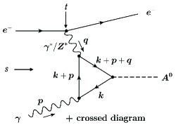
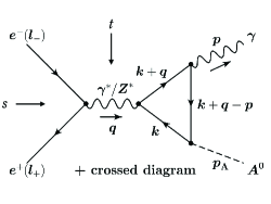
(a)                                                (b)

Figure 1: CP-odd Higgs $A^{0}$ production in (a) $e\gamma$ and (b) $e^{+}e^{-}$ collisions.

In our previous work on $e\gamma\to eA^{0}$ process [6], we introduced the spacelike TFF which is given by

$$F_{t}^{\ e\gamma\rightarrow eA^{0}}(\rho,\tau)=\frac{\tau}{1+\rho\tau}[g^{e\gamma}(\rho)+4f(\tau)]~{},$$ (2)

where the scaling variables $\rho$ and $\tau$ are defined as

$$\rho\equiv\frac{-q^{2}}{4m_{t}^{2}},\quad\tau\equiv\frac{4m_{t}^{2}}{m_{A}^{2}}\quad(q^{2}<0)~{},$$ (3)

with $m_{t}$ ($m_{A}$) being the top-quark ($A^{0}$ boson) mass, and the function $g^{e\gamma}(\rho)$ is given by

$$g^{e\gamma}(\rho) = \left[\log\frac{\sqrt{\rho+1}+\sqrt{\rho}}{\sqrt{\rho+1}-\sqrt{\rho}}\right]^{2}~{},$$ (4)

and $f(\tau)$ is the well-known function which appears in the Higgs decay process $H_{\rm SM}\rightarrow\gamma\gamma$ [8].

For $e\gamma\to eA^{0}$ process, $q^{2}$ is negative, while $q^{2}(=\sqrt{s})$ is positive for the process of $e^{+}e^{-}\to A^{0}\gamma$. For the latter case we introduce a timelike TFF as follows:

$$F_{t}^{\ e^{+}e^{-}\rightarrow\gamma A^{0}}(\rho,\tau)=\frac{\tau}{1-\rho\tau}[-g^{e^{+}e^{-}}(\rho)+4f(\tau)]~{},$$ (5)

where $g^{e^{+}e^{-}}(\rho)$ turns out to be

$$g^{e^{+}e^{-}}(\rho)=-\left[\log\frac{\sqrt{\rho}+\sqrt{\rho-1}}{\sqrt{\rho}-\sqrt{\rho-1}}-i\pi\right]^{2}~{},$$ (6)

and the scaling variables $\rho$ and $\tau$ are now defined as

$$\rho\equiv\frac{q^{2}}{4m_{t}^{2}},\quad\tau\equiv\frac{4m_{t}^{2}}{m_{A}^{2}}\quad(q^{2}>0)~{}.$$ (7)

In the expressions of (4) and (6), we make an analytic continuation by putting $+i\epsilon$ to $q^{2}$.

$$g^{e\gamma}\left(\frac{-q^{2}}{4m_{t}^{2}}-i\epsilon\right)=-g^{e^{+}e^{-}}\left(\frac{q^{2}}{4m_{t}^{2}}+i\epsilon\right)~{},$$ (8)

which leads to the following relation between the timelike and spacelike TTFs given as

$$F_{t}^{\ e\gamma\rightarrow eA^{0}}(-\rho,\tau) = \frac{\tau}{1-\rho\tau}[g^{e\gamma}(-\rho)+4f(\tau)]=\frac{\tau}{1-\rho\tau}[-g^{e^{+}e^{-}}(\rho)+4f(\tau)]$$ (9)

$$= F_{t}^{\ e^{+}e^{-}\rightarrow\gamma A^{0}}(\rho,\tau)~{}.$$

In Fig.2(a) we plot the real and imaginary parts of the TFF in the whole region from spacelike $q^{2}<0$ to timelike $q^{2}>0$ as a function of $\rho=q^{2}/4m_{t}^{2}$. As can be seen from the figure, the imaginary part (orange line) exhibits a cusp structure at $\rho=1$, which corresponds to the $t\bar{t}$ threshold, i.e, $q^{2}=(2m_{t})^{2}$, while the real part (blue line) changes sign at $\rho=1$.

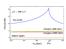
(a)                                                         (b)

Figure 2: Transition form factor for $A^{0}$ production in $e^{+}e^{-}$ collisions:(a) Real and imaginary parts of $F_{t}^{e^{+}e^{-}}(\rho,\tau)$ , and (b) Absolute value of $F_{f}^{e^{+}e^{-}}(\rho,\tau)$ for various fermion loops; top-quark, bottom-quark, chargino with mass 300 GeV and 1000 GeV.

The production cross section depends on the absolute square of the TFF and thus it shows a cusp structure at $\rho=1$ (see Fig.4(a) and (b)). In Fig.2(b), we show contributions to the absolute value of transition form factor $|F_{f}(s,m_{A}^{2},m_{f}^{2})|$ from the triangle one-loop diagram of fermion $f$; top-quark, bottom-quark and chargino with mass 300 GeV and 1000 GeV. As seen from the figure, the chargino and bottom-quark do not give sizable effects. The main contribution comes from the top-quark loop diagram. We also note that squarks do not contribute, since the trilinear $A^{0}$ coupling to mass-eigenstate squark pairs vanishes [6].

3 CP-odd Higgs $A^{0}$ production in $e^{+}e^{-}$ collisions

As a minimal extension of the Higgs sector of the SM, we consider the type-II 2HDM which includes the MSSM as a special case [8]. After the spontaneous symmetry breaking, there appear two charged $H^{\pm}$ and three neutral $h^{0}$, $H^{0}$ (CP-even), $A^{0}$ (CP-odd) Higgs bosons. The characteristics of $A^{0}$ couplings to other fields are as follows : 1) In contrast to the CP-even Higgs bosons $h^{0}$ and $H^{0}$, $A^{0}$ does not couple to $W^{+}W^{-}$ and $ZZ$ pairs at tree level. Hence $W$- and $Z$-boson one-loop diagrams do not contribute to the $A^{0}$ production. 2) $A^{0}$ does not couple to other two physical Higgs bosons in cubic interactions. 3) The couplings of $A^{0}$ to quarks and leptons are proportional to their masses. Therefore, we only consider the top-quark for the charged fermion loop diagrams. The $A^{0}$ coupling to the top-quark with mass $m_{t}$ is given by $\lambda\gamma_{5}$ with $\lambda=-gm_{t}\cot\beta/(2m_{W})$.

We investigate the $A^{0}$ production process: $e^{-}(l_{-})+e^{+}(l_{+})\rightarrow\gamma(p)+A^{0}(p_{A})$, where we detect the produced real photon in the final state. This process has been studied already in the literature [9]. Here we reconsider the process in the light of transition form factors. The one-loop diagrams which contribute to the reaction are classified into two groups: $\gamma^{*}$-exchange and $Z^{*}$-exchange diagrams (see Fig.1(b)). As we will see later, the contribution of the former is far more dominant over that of the latter. The scattering amplitude for each process turns out to be

$$\langle\gamma A^{0}|T|e^{-}e^{+}\rangle^{t}_{\gamma^{*}}=[\overline{v}(l_{+})(-ie\gamma^{\mu})u(l_{-})]\frac{-i}{q^{2}+i\epsilon}A_{\mu\nu}^{t}\epsilon^{\nu}(p)~{},$$ (10)

$$\langle\gamma A^{0}|T|e^{-}e^{+}\rangle^{t}_{Z^{*}}=\frac{g}{4\cos\theta_{W}}[\overline{v}(l_{+})(i\gamma^{\mu})(f_{Ze}+\gamma_{5})u(l_{-})]\frac{-i}{q^{2}-m_{Z}^{2}+i\epsilon}\widetilde{A}^{t}_{\mu\nu}\epsilon^{\nu}(p)~{},$$ (11)

with

$$A_{\mu\nu}^{t}=-\frac{e^{2}g}{(4\pi)^{2}}N_{C}q_{t}^{2}\frac{\cot\beta}{2m_{W}}F_{t}(\rho,\tau)\varepsilon_{\mu\nu\rho\sigma}q^{\rho}p^{\sigma}~{},$$ (12)

$$\widetilde{A}_{\mu\nu}^{t}=-\frac{eg^{2}}{(4\pi)^{2}}\frac{N_{C}q_{t}f_{Zt}}{4\cos\theta_{W}}\frac{\cot\beta}{2m_{W}}F_{t}(\rho,\tau)\varepsilon_{\mu\nu\rho\sigma}q^{\rho}p^{\sigma}~{},$$ (13)

where $u(l_{-})$ and $\overline{v}(l_{+})$ are the spinors for the electron and positron with momentum $l_{-}$ and $l_{+}$, respectively, $\epsilon^{\nu}(p)$ is the produced photon polarization vector with $p_{\nu}\epsilon^{\nu}(p)=0$, and $f_{Ze}=-1+4\sin^{2}\theta_{W}$ and $f_{Zt}=1-(8/3)\sin^{2}\theta_{W}$ are the strength of vector part of the $Z$-boson coupling to electron and top-quark, respectively, with $\theta_{W}$ being the Weinberg angle.

Adding two amplitudes given in Eqs.(10) and (11), we calculate the differential cross section for the $A^{0}$ production in $e^{+}e^{-}$ collisions with unpolarized initial beams, which is expressed by the sum of three terms:

$$\left(\frac{d\sigma}{dt}\right)_{\gamma^{*}}=\frac{\alpha_{\rm em}^{3}}{64\pi}\frac{g^{2}}{4\pi}\Bigl{(}\frac{\cot\beta}{2m_{W}}\Bigr{)}^{2}\frac{1}{s}\left(\frac{t^{2}+u^{2}}{s^{2}}\right)\Bigl{|}N^{t}_{C}q_{t}^{2}F_{t}(q^{2},m_{A}^{2},m_{t}^{2})\Bigr{|}^{2}~{},$$ (14)

$$\left(\frac{d\sigma}{dt}\right)_{Z^{*}}=\frac{\alpha_{\rm em}}{64\pi}\Bigl{(}\frac{g^{2}}{4\pi}\Bigr{)}^{3}\Bigl{(}\frac{\cot\beta}{2m_{W}}\Bigr{)}^{2}\Bigl{(}\frac{1}{16\cos^{2}\theta_{W}}\Bigr{)}^{2}\frac{s}{(s-m_{Z}^{2})^{2}}$$

$$\times f_{Zt}^{2}(f_{Ze}^{2}+1)\left(\frac{t^{2}+u^{2}}{s^{2}}\right)\Bigl{|}N^{t}_{C}q_{t}F_{t}(q^{2},m_{A}^{2},m_{t}^{2})\Bigr{|}^{2}~{},$$ (15)

$$\left(\frac{d\sigma}{dt}\right)_{\rm int}=-2\times\frac{\alpha^{2}_{\rm em}}{64\pi}\Bigl{(}\frac{g^{2}}{4\pi}\Bigr{)}^{2}\Bigl{(}\frac{\cot\beta}{2m_{W}}\Bigr{)}^{2}\frac{1}{16\cos^{2}\theta_{W}}\frac{1}{s-m_{Z}^{2}}$$

$$\times f_{Zt}f_{Ze}q_{t}\left(\frac{t^{2}+u^{2}}{s^{2}}\right)\Bigl{|}N^{t}_{C}q_{t}F_{t}(q^{2},m_{A}^{2},m_{t}^{2})\Bigr{|}^{2}~{},$$ (16)

where each corresponds to the contribution of the $\gamma^{*}$-exchange diagrams, the $Z^{*}$-exchange diagrams and their interference, respectively, and $\alpha_{\rm em}=e^{2}/4\pi$.

4 Numerical analysis of the cross sections

We analyze numerically the three differential cross sections given in Eqs.(14)-(16). We choose the parameters as follows: $m_{t}=173~{}{\rm GeV}$, $m_{Z}=91~{}{\rm GeV}$, $m_{W}=80~{}{\rm GeV}$, $\cos\theta_{W}={m_{W}}/{m_{Z}}$, $e^{2}=4\pi\alpha_{em}={4\pi}/{128}$, $g={e}/{\sin\theta_{W}}$. The electromagnetic constant $e^{2}$ is chosen to be the value at the scale of $m_{Z}$. For the above choice of parameters, we find $f_{Zt}f_{Ze}<0$ and, therefore, Eq.(16) shows that the interference between the $\gamma^{*}$- and $Z^{*}$-exchange diagrams work constructively and ${d\sigma_{({\rm Int})}}/{dt}$ is positive. For the remaining parameters, we assume $m_{A}$ between 200 GeV and 500 GeV and the moderate values for $\tan\beta$, which fall within the allowed region for the $(m_{A},\tan\beta)$ parameter space [10]. We plot these differential cross sections as a function of $t$ in Fig.3(a) for the case $\sqrt{s}=250$GeV, $m_{A}=200$GeV and $\cot\beta=1$. Note that the cross sections are proportional to $\cot^{2}\beta$. We find that the contribution from the s-channel $\gamma^{*}$-exchange diagrams is far more dominant over the ones from $Z^{*}$-exchange diagrams as well as from the interference term.

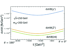
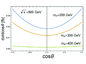
(a)                                                         (b)

Figure 3: Differential cross section for $A^{0}$ production in $e^{+}e^{-}$ collisions:(a) Three components of cross section and (b) $A^{0}$ mass dependence of differential cross section.

We observe that at $\sqrt{s}=250$ GeV, $m_{A}=200$ GeV  ($\sqrt{s}=500$ GeV, $m_{A}=300$ GeV), the ratio of $d\sigma_{Z^{*}}/dt$ to $d\sigma_{\gamma^{*}}/dt$ at $\theta=90^{\circ}$ is $5.94\times 10^{-2}\ (4.98\times 10^{-2})$ and $d\sigma_{{\rm int}}/dt$ to $d\sigma_{\gamma^{*}}/dt$ at $\theta=90^{\circ}$ is $4.43\times 10^{-2}$ $(3.98\times 10^{-2})$. As for the total cross section, for $m_{A}=300$ GeV, the ratio $\sigma_{\rm tot}(Z^{*})/\sigma_{\rm tot}(\gamma^{*})$ ($\sigma_{\rm tot}({\rm int})/\sigma_{\rm tot}(\gamma^{*})$)is $4.97\times 10^{-2}$ ($4.06\times 10^{-2}$) as shown in Fig.4(a). We also show the $m_{A}$ dependence of the differential and total cross sections in Fig.3(b) and in Fig.4(b), respectively.

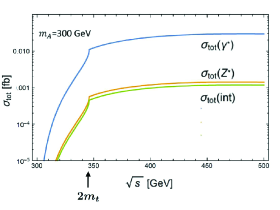
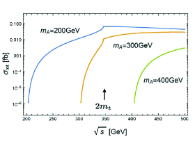
(a)                                                         (b)

Figure 4: Total cross section for $A^{0}$ production in $e^{+}e^{-}$ collisions:(a) Three components of cross section and (b) $A^{0}$ mass dependence of total cross section.

5 Box diagram contributions

Now let us consider under what conditions the TFF interpretation provides a good framework to describe the process. If the contribution from the triangle-loop diagrams is dominant over the one from the box-type diagrams, then the TFF leads to a good description of the process, where the production cross section is proportional to the absolute square of the TFF. The possible contributions coming from the box-type diagrams in the MSSM are the following: (a) Chargino-sneutrino box diagram and (b) Neutralino-selectron process shown in Fig.5. The former is the supersymmetric counterpart of the $W$-$\nu_{e}$ box diagram and the latter is the one of $Z$-electron box diagram, both of which are relevant in the case of $H_{\rm SM}\gamma$ production in $e^{+}e^{-}$ collisions. Of course it is difficult to cover all the parameter spaces for the masses and couplings of charginos and sneutrinos and for those of neutralinos and selectrons.

The one-loop box-diagram amplitude involving chargino $\tilde{\chi}_{i}^{+}$ ($i=1,2$) is given by

$$A_{e^{+}e^{-}\rightarrow\gamma A^{0}}^{(\tilde{\chi}\tilde{\nu})}=\left(\frac{eg^{3}\kappa_{1}|V_{11}|^{2}}{16\pi^{2}}\right)\frac{m_{\tilde{\chi}}}{4}\epsilon^{*}(p)^{\beta}\left[\overline{v}(l_{+})F_{(\tilde{\chi}\tilde{\nu})\beta}(1-\gamma_{5})u(l_{-})\right]~{}.$$ (17)

Since we are only interested in the order of magnitude for the $A^{0}$ production, we assume that the only mass eigenstate $\tilde{\chi}_{1}^{\pm}$ contributes dominantly and take $\kappa_{1}|V_{11}|^{2}\sim{\cal O}(1)$ for the coupling of $\tilde{\chi}_{1}^{\pm}$ to $A^{0}$. We can calculate the form factor $F_{(\tilde{\chi}\tilde{\nu})\beta}$ in terms of Passarino-Veltman’s scalar integrals[11]. This is obtained by interchanging $s$ and $t$ variables for the case of $e\gamma\to eA^{0}$ process [7]. Similar argument holds for the neutralino-selectron box contribution.

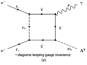
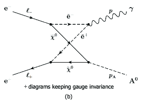
Figure 5: Possible box-diagrams in the MSSM: (a)Chargino($\tilde{\chi}^{-}$)-sneutrino($\tilde{\nu}_{e}$)-box contribution and (b)Neutralino($\tilde{\chi}^{0}$)-selectron($\tilde{e}^{-}$)-box contribution.

We show in Fig.6 the total cross section for the $A^{0}$ production in $e^{+}e^{-}\to A^{0}\gamma$ and compare the contribution from the box diagrams with the one from the top-quark-loop diagrams. For chargino with mass 300 GeV the chargino-sneutrino contribution is smaller than the one from top-quark by two order of magnitude. With chargino mass 1000 GeV the chargino-sneutrino contribution becomes much smaller by four order of magnitude. In addition the interference between top-quark-loop and box diagrams is found to be very small. The similar box-diagram contributions for the case $e\gamma\to eA^{0}$ were studied in [7], and they were found to be small.

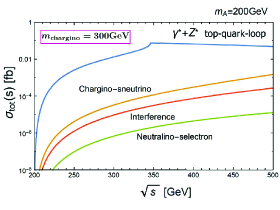
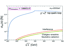
(a)                                                         (b)

Figure 6: Top-quark vs. box-diagrams contributions:(a) mass of chargino 300 GeV and (b)mass of chargino 1000 GeV.

6 Conclusion

In this talk we have studied the production of CP-odd Higgs boson $A^{0}$ associated with a real photon in $e^{+}e^{-}$ collisions in terms of the timelike TFF. The dominant contribution is coming from the top-quark one-loop diagrams. The $\gamma^{*}$ process is far more dominant over $Z^{*}$ process. The box-diagram contributions, from chargino-sneutrino and neutralino-selectron related processes, do not give sizable effects in the parameter space of masses and couplings we have studied. If $\tan\beta$ is not large and chargino is very heavy their contributions are negligible. Then at the electroweak one-loop level, the TFF provides a good description of the process. Finally, what about the QCD radiative corrections to the top-quark one-loop diagram? As is well known, for $m_{t}\gg m_{A}$, though it does not apply to our case, the QCD corrections to the effective $A\gamma\gamma$ coupling are absent. In the case of $e^{+}e^{-}\to H_{\rm SM}\gamma$, the NLO QCD effects are known to be rather small [12], which would suggest that a similar situation occurs in our present case. Of course, more detailed analyses should be carried out.

References

-
[1]
ATLAS Collaboration,Observation of a new particle in the search for
the Standard Model Higgs boson with the ATLAS detector at the LHC,
Phys. Lett. B716, 1 (2012), doi:10.1016/j.physletb.2012.08.020;
CMS Collaboration, Observation of a New Boson at a Mass of 125 GeV with the CMS Experiment at the LHC,Phys. Lett. B716, 30 (2012),doi:10.1016/j.physletb.2012.08.021. -
[2]
ATLAS Collaboration, Measurements of Higgs boson production and couplings
in diboson final states with the ATLAS detector at the LHC,Phys. Lett. B726, 88 (2013), doi:10.1016/j.physletb.2014.05.011;Evidence for the spin-0 nature of the Higgs boson using ATLAS data,
Phys. Lett. B726, 120 (2013),doi:10.1016/j.physletb.2013.08.026.
CMS Collaboration, Study of the mass and spin-parity of the Higgs boson candidate via
its decays to Z boson pairs, Phys. Rev. Lett. 110, 081803(2013),
doi:10.1103/PhysRevLett.110.081803. - [3] http://www.linearcollider.org.
- [4] N. Watanabe, Y. Kurihara, K. Sasaki and T. Uematsu, Higgs Production in Two-Photon Process and Transition Form Factor, Phys. Lett. B728, 202 (2014),doi:10.1016/j.physletb.2013.11.051.
- [5] N. Watanabe, Y. Kurihara, T. Uematsu, and K. Sasaki, Higgs boson production in and real collisions, Phys. Rev. D90, 033015 (2014), doi:10.1103/PhysRevD.90.033015.
- [6] K. Sasaki and T. Uematsu, CP-odd Higgs boson production in collision,Phys. Lett. B781, 290 (2018),doi:10.1016/j.physletb.2018.04.005.
- [7] K. Sasaki and T. Uematsu, CP even and odd Higgs boson production in electron-photon collisions, PoS RADCOR2019 (2019) 021, doi:10.22323/1.375.0021.
- [8] J. F. Gunion, H. E. Haber, G. Kane and S. Dawson, The Higgs Hunter’s Guide (Addison-Wesley, 1990).
- [9] A. Djouadi, V. Driesen, W. Hollik and J. Rosiek, Associated production of Higgs bosons and a photon in high-energy collisions,Nucl. Phys. B491, 68 (1997), doi:10.1016/S0550-3213(96)00711-0.
- [10] Particle Data Group Collaboration (P. A. Zyla et al.), Review of Particle Physics, PTEP2020 no. 8, (2020) 083C01, doi:10.1093/ptep/ptaa104.
- [11] G. Passarino and M. Veltman, One loop corrections for annihilation into in the Weinberg Model, Nucl. Phys. B160, 151 (1979),doi:10.1016/0550-3213(79)90234-7.
- [12] W.-L.Sang, W. Chen, F. Feng, Y. Jia, Q.-F. Sun, Next-to-leading-order QCD corrections to , Phys.Lett. B775, 152 (2017),doi:10.1016/j.physletb.2017.10.044.