Effective Dynamics of Tracer in Active Bath: A Mean-field Theory Study

Abstract

We develop a theoretical framework to study the effective dynamics of a tracer immersed in a nonequilibrium bath consisting of active particles. By using a mean-field approximation and extending the linearized Dean equation to nonequilibrium environment, we derive a generalized Langevin equation for the tracer particle, wherein colored noise terms and a memory kernel reflect the roles of interactions between tracer and bath particles as well as activity of the bath. In particular, we obtain a self-consistent equation to calculate the long time diffusion coefficient and mobility of tracer, finding that they both increase non-linearly with bath activity, in good consistents with direct simulation results.

I Introduction

Tracer dynamics in nonequilibrium baths have attracted great attention in recent decades[1, 2, 3, 4, 5, 6, 7], which is an important topic for understanding many biological processes and artificial active particles systems[1, 8, 9, 10, 11]. For instance, complex intracellular environment can be abstracted as an active bath, since the molecular motors in cytoplasm are similar to active particles. Consequently, biomolecules in living cells often show anomalous behaviors (such as anomalous diffusion) due to this nonequilibrium feature[12]. Besides, the presence of active fluctuations may promote protein folding, which has been observed in a polymer model system[13]. On the other hand, the passive tracers in a bath of swimming bacteria show novel properties such as superdiffusion[1], effective attractive interactions[9], and even targeted delivery[14]. Because of the importance and wide range of applications, developing a general theoretical framework to describe the dynamics of tracer in such nonequilibrium baths is desirable.

In this regard, some important progresses have been made in recent years[15, 16, 17, 18, 19, 20, 21, 22, 23, 24, 25], including density functional theory[15], nonequilibrium linear response theory[23, 16, 19, 18, 22, 24, 25], mean-field theory[20, 17, 26, 27, 28], and even mode-coupling theory[29, 30]. For instance, Speck and Seifert et al established a fluctuation-dissipation theorem (FDT) in nonequilibrium steady state of sheared colloidal suspension system[2, 31], then studied the mobility and diffusivity of a tagged particle in such system[31]. Starting from a different path, Brady et al used Smoluchowski equation to investigate the long-time diffusivity of a tracer submerged in active suspensions[23, 6], and further derived a general relationship between diffusivity and mobility by testing the results with Stokes-Einstein-Sutherland relation[6]. In the fundamental respect, Maes et al obtained a generalized fluctuation-dissipation relation (FDR) for the linear response of driven systems[16, 18], studied the effective dynamics of Brownian particle with strong interaction with the medium, and extended this FDR to non-equilibrium systems with memory [19]. Most recently, they used their method to derive the fluctuation dynamics of a probe in weak coupling with an active environment such as living tissue[24].

In the present article, we propose an alternative theoretical method based on mean-field theory to study the effective dynamics of tracer in active bath. Starting from the Langevin equations (LEs) for the whole system, we achieve the linearized Dean’s equation [32] for the evolution of density fluctuation of bath particles, wherein the interactions between tracer and bath particles are involved explicitly. By substituting the density fluctuation into the tracer’s LE, we derive a generalized Langevin equation (GLE) for tracer, which includes a memory kernel function and complex effective noise terms, of which the correlations of such noises are strongly coupled with tracer dynamics. This GLE facilitates us to calculate the effective diffusion and mobility of the tracer. With an appropriate approximation, these transport coefficients can be conveniently calculated through self-consistent equations, showing good agreements with direct molecular dynamics simulation data.

This article is organized as following. In Sec.II we derive the Dean’s equation for bath density fluctuation and the GLE for tracer. In Sec.III we use the GLE to calculate the effective diffusion coefficient and mobility of the tracer, and compare them with simulation results. Details of the derivations are shown in Appendix A.

II Model and Theory

II.1 Equations of Motion

In the present work, we consider a two-dimensional (2D) system composed of a spherical passive tracer of radius $R_{tr}$ surrounded by $N$ self-propelled active bath particles of radius $R_{b}$, both in a background equilibrium thermal bath with temperature $T$. The tracer position is denoted by ${\bf x}$ and those of the bath particles are given by ${\bf r}_{i=\left(1,...N\right)}$. The dynamics of the tracer are described by the overdamped Langevin equation

$${\rm d}{\bf x}=-\mu_{t}\nabla_{{\bf x}}\sum_{i}U\left(\left|{\bf r}_{i}-{\bf x}\right|\right){\rm d}t+\sqrt{2\mu_{t}T}{\rm d}{\bf W}_{x},$$ (1)

where $\mu_{t}$ is the bare mobility of tracer, $U\left(\left|{\bf r}_{i}-{\bf x}\right|\right)$ is the pair interaction potential between the tracer and bath particle $i$, ${\bf W}_{x}$ denotes a standard Wiener process accounting for thermal noise such that $dW_{x}\left(t\right)=\xi\left(t\right)dt$ with $\left\langle\xi\left(t\right)\right\rangle=0$ and $\left\langle\xi\left(t\right)\xi\left(t^{\prime}\right)\right\rangle=\delta\left(t-t^{\prime}\right)$. For the bath particles, we model the self-propulsion force by the Ornstein-Uhlenbeck (OU) noise [33], therefore the dynamics are given by

$${\rm d}{\bf r}_{i}= -\mu_{b}\nabla_{i}\left[\sum_{j\neq i}V\left(\left|{\bf r}_{i}-{\bf r}_{j}\right|\right)+U\left(\left|{\bf r}_{i}-{\bf x}\right|\right)\right]{\rm d}t$$

$$+{\bf f}_{i}{\rm d}t+\sqrt{2\mu_{b}T}{\rm d}{\bf W}_{i},$$ (2)

where $\mu_{b}$ is the bare mobility of bath particles, $V\left(\left|{\bf r}_{i}-{\bf r}_{j}\right|\right)$ is the interacting potential between bath particles $i$ and $j$, and ${\bf W}_{i}$ accounts for thermal noise for particle $i$. Active force ${\bf f}_{i}$ is the OU-colored noise type, governed by

$$\tau_{b}{\rm d}{\bf f}_{i}=-{\bf f}_{i}{\rm d}t+\sqrt{2D_{b}}{\rm d}{\bf W}_{i}^{f},$$ (3)

where $\tau_{b}$ denotes the persistent time of self-propulsion, $D_{b}$ is an equivalent diffusion coefficient, and ${\bf W}_{i}^{f}$ is also a standard Wiener process. The time correlation of ${\bf f}_{i}$ is then given by

$$\left\langle{\bf f}_{i}\left(t\right){\bf f}_{j}\left(t^{\prime}\right)\right\rangle=\frac{D_{b}}{\tau_{b}}\delta_{ij}e^{-\left|t-t^{\prime}\right|/\tau_{b}}{\bf I}$$ (4)

wherein $i(j)$ stands for particle label and ${\bf I}$ is unit tensor. The model used here for the active particles is known as the AOUP model. Note that in many studies[34, 4, 35], the active Brownian particle(ABP) model is also often used, wherein the active force is realized via a constant velocity $v_{0}$ along a random rotational direction given by ${\bf e}_{\varphi}=\left(\cos\varphi,\sin\varphi\right)$, where $\left\langle\dot{\varphi}\left(t\right)\dot{\varphi}\left(t^{\prime}\right)\right\rangle=2D_{r}\delta\left(t-t^{\prime}\right)$ with $D_{r}$ the rotational diffusion coefficient. It can be shown that the correlation function of the active force of ABP model at a coarse-grained time scale is the same in form as that of AOUP model. To better illustrate our model, we have shown a schematic diagram of the system in Fig. 1.

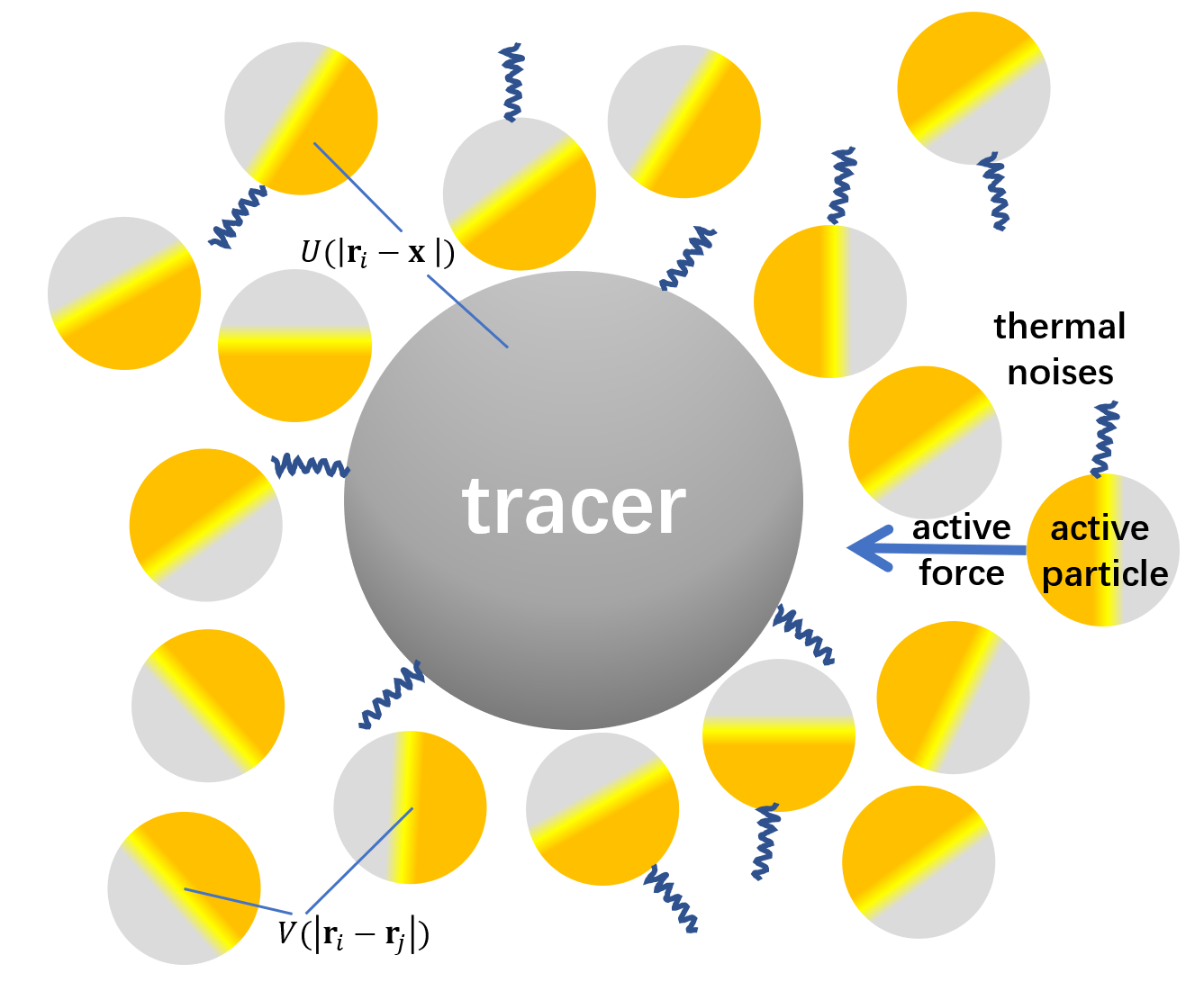
Figure 1: Schematic figure of the model system. The bath particles are active and the tracer is passive and the size is larger than that of the bath particles. Both of them are immersed in the background equilibrium reservoir, therefore influenced by thermal white noises.

II.2 Density Fluctuation of Active Bath: Mean field approximation

The goal of the present work is to obtain an effective (reduced) equation of motion for the tracer particle, by tracing out the degrees of freedom of the bath particles. To this end, one needs to compute the force exerted by the bath particles on the tracer in a mean-field manner. Following the procedures as described in [36], we first describe the bath dynamics at a coarse-grained level, by introducing the bath density field $\rho\left({\bf r},t\right)=\sum_{i}\rho_{i}\left({\bf r},t\right)$ where $\rho_{i}({\bf r},t)=\delta\left({\bf r}-{\bf r}_{i}\left(t\right)\right)$, and using standard techniques [36] to derive the time evolution equation (see appendix for details),

$$\frac{\partial\rho\left({\bf r},t\right)}{\partial t}= \mu_{b}\nabla\cdot\left\{\rho\left({\bf r},t\right)\Big{[}\int{\rm d}{\bf r}^{\prime}\rho\left({\bf r}^{\prime},t\right)\nabla V\left(\left|{\bf r}-{\bf r}^{\prime}\right|\right)+\nabla U\left(\left|{\bf r}-{\bf x}\right|\right)\Big{]}\right\}$$

$$+\mu_{b}T\nabla^{2}\rho\left({\bf r},t\right)+\nabla\cdot\left(\sqrt{\rho\left({\bf r},t\right)}\boldsymbol{\xi}^{T}\right)+\nabla\cdot\left(\sqrt{\rho\left({\bf r},t\right)}\boldsymbol{\xi}^{A}\right)$$ (5)

where $\boldsymbol{\xi}^{T}$ and $\boldsymbol{\xi}^{A}$ are spatiotemporal Gaussian noises, with correlations

$$\left\langle\boldsymbol{\xi}^{T}\left({\bf r},t\right)\boldsymbol{\xi}^{T}\left({\bf r}^{\prime},t^{\prime}\right)\right\rangle=2\mu_{b}T\delta\left(t-t^{\prime}\right)\delta\left({\bf r}-{\bf r}^{\prime}\right){\bf I}$$ (6)

and

$$\left\langle\boldsymbol{\xi}^{A}\left({\bf r},t\right)\boldsymbol{\xi}^{A}\left({\bf r}^{\prime},t^{\prime}\right)\right\rangle=\frac{D_{b}}{\tau_{b}}e^{-\left|t-t^{\prime}\right|/\tau_{b}}\delta\left({\bf r}-{\bf r}^{\prime}\right){\bf I}$$ (7)

respectively.

On the right-hand-side of Eq.(5), the first term describes how the interactions $U$(particle-tracer) and $V$(particle-particle) would influence the density field. The second term is a diffusive one that accounts for the background thermal noise at temperature $T$. In the third term, $\boldsymbol{\xi}^{T}$ (’T’ for thermal) denotes a coarse-grained white noise, which also originates from the thermal background, coupled with the density field itself. $\boldsymbol{\xi}^{A}$ (’A’ for active) in the fourth term denotes a coarse-grained OU-noise resulting from the coupling between the active forces ${\bf f}_{i}$ and the density field, which would be absent for a passive bath.

To proceed further, we assume that the system is nearly homogeneous(i.e. no phase separation or dynamic heterogeneous) and thus the bath dynamics is mainly dependent on the density fluctuation $\delta\rho\left({\bf r},t\right)=\rho\left({\bf r},t\right)-\bar{\rho}$, where $\bar{\rho}$ is the number density of bath particles. Using the methods in Ref.[32, 20](also shown in Appendix A.1), on the condition of weak interaction and high density, the mean-field approximation is applicable and one can solve the linearized equation of bath density fluctuation in Fourier space

$$\partial_{t}\delta\rho_{k}(t)\approx -\mu_{b}k^{2}\left[\bar{\rho}U_{k}e^{i{\bf k}\cdot{\bf x}}+\left(T+\bar{\rho}V_{k}\right)\delta\rho_{k}(t)\right]$$

$$+\sqrt{\bar{\rho}}i{\bf k}\cdot\left[\tilde{\boldsymbol{\xi}}_{k}^{T}\left(t\right)+\tilde{\boldsymbol{\xi}}_{k}^{A}\left(t\right)\right]$$ (8)

where $\delta\rho_{k}\left(t\right)=\int\delta\rho\left({\bf r},t\right)e^{i{\bf k}\cdot{\bf r}}{\rm d}{\bf r}$ is the Fourier mode of density fluctuation $\delta\rho\left({\bf r},t\right)$ (isotropic condition has been used such that $\delta\rho_{{\bf k}}$ only depends on $k=\left|{\bf k}\right|$), and $V_{k}$ , $U_{k}$, $\tilde{\boldsymbol{\xi}}_{k}^{T}\left(t\right)$ and $\tilde{\boldsymbol{\xi}}_{k}^{A}\left(t\right)$ are Fourier modes defined in the same manner for $V\left(r\right)$, $U\left(r\right)$, $\boldsymbol{\xi}^{T}\left(t\right)$ and $\boldsymbol{\xi}^{A}\left(t\right)$ respectively. The formal solution of (8) is then given by

$$\delta\rho_{k}(t)\approx\int_{-\infty}^{t}{\rm d}se^{-(t-s)/a_{k}}\left[-\mu_{b}k^{2}\bar{\rho}U_{k}e^{i{\bf k}\cdot{\bf x}\left(s\right)}\right.\\ \left.+i\sqrt{\bar{\rho}}{\bf k}\cdot\left(\tilde{\boldsymbol{\xi}}_{k}^{T}\left(s\right)+\tilde{\boldsymbol{\xi}}_{k}^{A}\left(s\right)\right)\right],$$ (9)

where $a_{k}=\left[\mu_{b}k^{2}\left(T+\bar{\rho}V_{k}\right)\right]^{-1}$ is a characteristic relaxation time scale depending on $k$ and the interaction potential $V$ among bath particles. Generally, $a_{k}$ scales as $k^{-2}$ so that fluctuations with short wavelength decays very fast.

II.3 Generalized Langevin Equation of Tracer

Now we turn to the tracer dynamics. Using the identity(proceeding the Fourier transform twice)

$$\nabla_{x}\sum_{i}U\left(\left|{\bf r}_{i}-{\bf x}\right|\right)=-\int_{{\bf k}}i{\bf k}e^{-i{\bf k}\cdot{\bf x}}\delta\rho_{k}U_{k}$$ (10)

where $\int_{{\bf k}}=\left(2\pi\right)^{-d}\int{\rm d}k^{d}$ is the integral over entire k-space, and inserting the formal solution of $\delta\rho_{k}$, Eq.(9), into Eq.(1), we can obtain a generalized Langevin equation (GLE) of the tracer

$$\dot{{\bf x}}\left(t\right)= \mu_{t}\int_{-\infty}^{t}{\bf F}\left({\bf x}\left(t\right)-{\bf x}\left(s\right),t-s\right){\rm d}s$$

$$+\boldsymbol{\eta}_{A}\left({\bf x}\left(t\right),t\right)+\boldsymbol{\eta}_{T}\left({\bf x}\left(t\right),t\right)+\sqrt{2\mu_{t}T}\boldsymbol{\xi}_{t},$$ (11)

where

$${\bf F}\left({\bf x}\left(t\right)-{\bf x}\left(s\right),t-s\right)$$

$$= -\mu_{b}\bar{\rho}\int_{{\bf k}}i{\bf k}k^{2}U_{k}^{2}e^{-i{\bf k}\cdot\left[{\bf x}\left(t\right)-{\bf x}\left(s\right)\right]}e^{-\left(t-s\right)/a_{k}}$$ (12)

is a memory kernel term, $\boldsymbol{\xi}_{t}={\rm d}{\bf W}_{x}\left(t\right)/{\rm d}t$ is the original thermal noise of the background equilibrium bath upon the tracer, and $\boldsymbol{\eta}_{A,T}\left({\bf x}(t),t\right)$ are complicated colored noises that account for the effects of active bath particles. In other words, the total force exerted by the bath particles on the tracer now is decomposed into a systematic frictional force with memory and a noise term, similar to that of a Brownian particle in a thermal bath. Nevertheless, now the noise terms $\boldsymbol{\eta}_{A,T}\left({\bf x}(t),t\right)$ are much more complicated than a simple Gaussian white one,

$$\boldsymbol{\eta}_{A,T}\left({\bf x}\left(t\right),t\right)= -\mu_{t}\int_{{\bf k}}{\bf k}e^{-i{\bf k}\cdot{\bf x}_{t}}U_{k}\int_{-\infty}^{t}e^{-\left(t-s\right)/a_{k}}$$

$$\times\left[\sqrt{\bar{\rho}}{\bf k}\cdot\tilde{\boldsymbol{\xi}}_{k}^{A,T}\left(s\right)\right]{\rm d}s$$ (13)

originated further from the coarse-grained thermal noise $\boldsymbol{\xi}^{T}$ or the coarse-grained active OU-noise $\boldsymbol{\xi}^{A}$, respectively (the correlation functions of $\boldsymbol{\xi}^{T}$ and $\boldsymbol{\xi}^{A}$ are given in Eq.(6) and Eq.(7), and $\boldsymbol{\eta}_{A,T}(t)$ can be seen as weighted sum of $\tilde{\boldsymbol{\xi}}_{k}^{A,T}\left(s\right)$ for all $s<t$). It is $\boldsymbol{\eta}_{A}\left({\bf x}\left(t\right),t\right)$ that accounts for the active nature of the bath, which becomes zero when activity is absent. Note that the structure of Eq.(13) is complicated, such that the properties of $\boldsymbol{\eta}_{A,T}$ are quite non-trivial.

Keeping to the lowest order, we can approximately write the memory kernel ${\bf F}\left({\bf x}\left(t\right)-{\bf x}\left(s\right),t-s\right)$ into a more familiar form as

$$\int_{-\infty}^{t}\mu_{t}{\bf F}\left({\bf x}\left(t\right)-{\bf x}\left(s\right),t-s\right){\rm d}s \simeq-\int_{-\infty}^{t}{\rm d}u\zeta(t-u)\dot{{\bf x}}(u)$$ (14)

(see Appendix A.2 for details), wherein the usual memory kernel $\zeta\left(t\right)$ reads,

$$\zeta(t)=\frac{\mu_{t}\mu_{b}\bar{\rho}}{d}\int_{{\bf k}}k^{4}U_{k}^{2}a_{k}e^{-t/a_{k}}$$ (15)

Consequently, the GLE for the tracer dynamics reads

$$\dot{{\bf x}}=-\int_{-\infty}^{t}\zeta(t-u)\dot{{\bf x}}(u){\rm d}u+\boldsymbol{\eta}_{A}\left(t\right)+\boldsymbol{\eta}_{T}\left(t\right)+\sqrt{2\mu_{t}T}\boldsymbol{\xi}_{t}$$ (16)

This equation is one of the main results of the present paper. It allows us to calculate the transport properties of tracer in active bath, such as mobility and diffusivity, and moreover to investigate the nature of active bath itself.

If one wants to investigate the long time behavior of the tracer, such as diffusion dynamics, the memory effect in the GLE could be ignored, such that one may adopt Markovian approximation as[37]

$$\int_{-\infty}^{t}\zeta(t-u)\dot{{\bf x}}(u){\rm d}u\simeq\left(\int_{0}^{\infty}\zeta(u){\rm d}u\right)\dot{{\bf x}}(t)\equiv\lambda\dot{{\bf x}}(t)$$ (17)

with explicitly the effective friction coefficient $\lambda$ reads

$$\lambda =\int_{0}^{\infty}\zeta(u){\rm d}u=\frac{\mu_{t}\mu_{b}\bar{\rho}}{d}\int_{{\bf k}}k^{4}U_{k}^{2}a_{k}$$

$$=\frac{\mu_{t}\bar{\rho}}{\mu_{b}d}\int_{{\bf k}}\frac{U_{k}^{2}}{\left(T+\bar{\rho}V_{k}\right)^{2}}.$$ (18)

Therefore, the GLE reduces to a simple Langevin equation(LE) with colored noise

$$\left(1+\lambda\right)\dot{{\bf x}}=\boldsymbol{\eta}_{A}\left(t\right)+\boldsymbol{\eta}_{T}\left(t\right)+\sqrt{2\mu_{t}T}\boldsymbol{\xi}_{t}$$ (19)

which serves as the working equation to study the diffusion dynamics of the tracer.

II.4 Noise Correlations

Previously, in most studies, the effect of the active bath on the tracer is treated as an additive noise with Ornstein-Uhlenbeck (OU) [1, 7, 38, 10, 39] type, wherein the amplitude and relaxation parameter are obtained through simulation or experimental data. Indeed, in certain aspects such as long-time diffusion and spatial distribution of the tracer in trapping potential, this approximation accords with the experimental or simulation results. However, how interparticle interactions and bath activity enter into such noise explicitly and how to derive the expression for such complex effects are still unclear as far as we know. In other words, the mechanism of noise generation is still unresolved from a theoretical point of view. In this respect, our theory provides an inspired understanding of this issue.

To investigate such noise properties, we use Eq.(16) as the starting point for further studies. Clearly, the dynamics of ${\bf x}$ strongly depends on the correlation property of the colored noises $\boldsymbol{\eta}_{T}\left(t\right)$ and $\boldsymbol{\eta}_{A}\left(t\right)$. After some straightforward calculations(see Appendix(A.3)), we have

$$\left\langle\boldsymbol{\eta}_{T}\left(t\right)\cdot\boldsymbol{\eta}_{T}\left(t^{\prime}\right)\right\rangle$$

$$\approx \mu_{t}^{2}\mu_{b}\bar{\rho}T\int_{{\bf k}}k^{4}U_{k}^{2}a_{k}\left\langle e^{-i{\bf k}\cdot\left[{\bf x}(t)-{\bf x}(t^{\prime})\right]}\right\rangle e^{-\left|t-t^{\prime}\right|/a_{k}}$$ (20)

and

$$\left\langle\boldsymbol{\eta}_{A}\left(t\right)\cdot\boldsymbol{\eta}_{A}\left(t^{\prime}\right)\right\rangle\approx\mu_{t}^{2}D_{b}\bar{\rho}\int_{{\bf k}}k^{4}U_{k}^{2}\left\langle e^{-i{\bf k}\cdot\left[{\bf x}(t)-{\bf x}(t^{\prime})\right]}\right\rangle$$

$$\times\frac{1}{\left(\tau_{b}/a_{k}\right)^{2}-1}\left[\tau_{b}e^{-\left|t-t^{\prime}\right|/\tau_{b}}-a_{k}e^{-\left|t-t^{\prime}\right|/a_{k}}\right]$$ (21)

It is observed that the noise correlations depend on the interactions $U$(between bath and tracer) and $V$(between active bath particles). In addition, they are also coupled with the tracer dynamics ${\bf x}\left(t\right)$.

To proceed, we need to know the information of correlation $\left\langle e^{-i{\bf k}\cdot\left[{\bf x}(t)-{\bf x}(t^{\prime})\right]}\right\rangle$. In the short time limit, one may adopt the so-called “adiabatic approximation” due to the time-scale separation between the tracer motion and bath particle dynamics, such that the tracer motion is not apparent and

$$\left\langle e^{-i{\bf k}\cdot\left({\bf x}_{t}-{\bf x}_{t^{\prime}}\right)}\right\rangle\approx 1.$$ (22)

In this case, we have

$$\left\langle\boldsymbol{\eta}_{A}\left(t\right)\cdot\boldsymbol{\eta}_{A}\left(t^{\prime}\right)\right\rangle\approx\mu_{t}^{2}D_{b}\bar{\rho}\int_{{\bf k}}\frac{k^{4}U_{k}^{2}}{\left(\tau_{b}/a_{k}\right)^{2}-1}$$

$$\times\left[\tau_{b}e^{-\left|t-t^{\prime}\right|/\tau_{b}}-a_{k}e^{-\left|t-t^{\prime}\right|/a_{k}}\right]$$ (23)

and

$$\left\langle\boldsymbol{\eta}_{T}\left(t\right)\cdot\boldsymbol{\eta}_{T}\left(t^{\prime}\right)\right\rangle\approx\mu_{t}^{2}\mu_{b}\bar{\rho}T\int_{{\bf k}}k^{4}U_{k}^{2}a_{k}e^{-\left|t-t^{\prime}\right|/a_{k}}.$$ (24)

Note that the latter one is proportional to the memory kernel in the GLE, Eq.(16), i.e.,

$$\left\langle\boldsymbol{\eta}_{T}\left(t\right)\cdot\boldsymbol{\eta}_{T}\left(t^{\prime}\right)\right\rangle=d\mu_{t}T\zeta\left(t-t^{\prime}\right).$$ (25)

Therefore, in the absence of activity (not considering the active part $\boldsymbol{\eta}_{A}$), fluctuation-dissipation theorem(FDT) holds among the systematic (memory) part and noisy part of the total force exerted by the bath particles on the tracer, reminiscent of the usual Brownian motion. Surely, in the presence of particle activity, $\boldsymbol{\eta}_{A}$ takes effect and the conventional FDT does not hold anymore since the system is far from equilibrium.

Nevertheless, if long time dynamics is involved, such adiabatic approximation is not valid. Noise correlations thus become quite complicated, depending on the behavior of $\left\langle e^{-i{\bf k}\cdot\left[{\bf x}(t)-{\bf x}(t^{\prime})\right]}\right\rangle$. In the next section, we will mainly study the diffusion behavior of the tracer particle. For that purpose, one may use “Gaussian approximation”, i.e., the tracer displacement within a time interval $t-t_{0}$ is Gaussian distributed with variance $2D_{\text{eff}}\left(t-t_{0}\right)$, such that

$$\left\langle e^{-i{\bf k}\cdot\left[{\bf x}(t)-{\bf x}(t_{0})\right]}\right\rangle\approx e^{-\frac{k^{2}}{2}\left\langle\Delta{\bf x}^{2}(t)\right\rangle}=e^{-k^{2}dD_{{\rm eff}}\left(t-t_{0}\right)}$$ (26)

wherein $\left\langle\Delta{\bf x}^{2}(t)\right\rangle=\left\langle\left[{\bf x}\left(t\right)-{\bf x}\left(0\right)\right]^{2}\right\rangle$ is the mean square displacement and $D_{\text{eff}}$ is the effective (long time) diffusion coefficient of the tracer. Note however, $D_{\text{eff}}$ must be calculated from the tracer dynamics, which in turn depends on the noise property and thus $D_{\text{eff}}$ itself. Therefore, $D_{\text{eff}}$ should be calculated in a self-consistent way, which will be discussed in the next section.

III Tracer Diffusion and Mobility

In this section, we will investigate the long-time diffusion coefficient $D_{\text{eff}}$ of the tracer. According to the Green-Kubo relation,

$$D_{{\rm eff}}= \lim_{t\rightarrow\infty}\frac{1}{2dt}\left\langle\Delta{\bf x}^{2}(t)\right\rangle=\frac{1}{d}\int_{0}^{\text{$\infty$}}{\rm d}t\left\langle\dot{{\bf x}}(t)\cdot\dot{{\bf x}}(0)\right\rangle$$ (27)

As already mentioned above, it is feasible to adopt the Markovian approximation and the dynamics of ${\bf x}$ is governed by Eq.(19) $\dot{{\bf x}}_{t}=\left(1+\lambda\right)^{-1}\left(\boldsymbol{\eta}_{A}+\boldsymbol{\eta}_{T}+\sqrt{2\mu_{t}T}\boldsymbol{\xi}_{t}\right)$. Substitute this into Eq.(27), one may calculate $D_{\text{eff}}$ straightforwardly given the noise correlations of $\boldsymbol{\eta}_{A}$ and $\boldsymbol{\eta}_{T}$. Nevertheless, as shown in Eqs.(20) and (21), the noise correlations may depend on the dynamics of ${\bf x}$ itself, thus proper approximations must be employed.

III.1 Adiabatic Approximation

If one simply uses the “naive” adiabatic approximation, Eq.(22), the subsequent noise correlations are given by Eqs.(23) and (24). One can thus obtain that

$$D_{\text{naive}} =\frac{1}{d\left(1+\lambda\right)^{2}}\left(I_{1}^{\text{ad}}+I_{2}^{\text{ad}}+d\mu_{t}T\right)$$

$$=\frac{1}{1+\lambda}\left(\mu_{t}T+\frac{\lambda}{1+\lambda}\mu_{T}\left(\frac{D_{b}}{\mu_{b}}\right)\right)$$ (28)

where

$$I_{1}^{\text{ad}}= \int_{0}^{\infty}\left\langle\boldsymbol{\eta}_{A}\left(0\right)\cdot\boldsymbol{\eta}_{A}\left(t\right)\right\rangle{\rm d}t=\mu_{t}^{2}D_{b}\bar{\rho}\int_{{\bf k}}k^{4}U_{k}^{2}a_{k}$$

$$= d\mu_{t}\lambda\left(D_{b}/\mu_{b}\right)$$ (29)

and

$$I_{2}^{\text{ad}}=\int_{0}^{\infty}\left\langle\boldsymbol{\eta}_{T}\left(0\right)\cdot\boldsymbol{\eta}_{T}\left(t\right)\right\rangle{\rm d}t=d\mu_{t}T\lambda,$$ (30)

and use has been made $\int_{0}^{\infty}\left\langle\boldsymbol{\xi}_{T}\left(0\right)\cdot\boldsymbol{\xi}_{T}\left(t\right)\right\rangle{\rm d}t=d$. The meaning of each term in Eq.(28) is clear. The first term, $\mu_{t}T/\left(1+\lambda\right)$, gives the diffusivity of the particle in a purely passive bath, wherein $\lambda$ accounts for the excess friction that results from the interactions $U$ between tracer and bath particles. The second term, $\left(D_{b}\mu_{t}/\mu_{b}\right)\lambda/\left(1+\lambda\right)^{2}$, arises from the activity of the bath particles. One can see that $D_{b}/\mu_{b}$ acts as an effective temperature of the bath, which contributes an active part to the total diffusion. However, as discussed above, this approximation should only be valid for short time. Therefore, $D_{\text{naive}}$ only serves as the zero-order approximation of the long-time diffusion constant.

III.2 Gaussian Approximation

A better approximation would be the Gaussian one described in Eq.(26), wherein $\left\langle e^{-i{\bf k}\cdot\left[{\bf x}(t)-{\bf x}(0)\right]}\right\rangle\simeq e^{-k^{2}dD_{{\rm eff}}t}$. Using this approximation, one can obtain the noise correlations as follows,

$$\left\langle\boldsymbol{\eta}_{T}\left(0\right)\cdot\boldsymbol{\eta}_{T}\left(t\right)\right\rangle\approx\mu_{t}^{2}\mu_{b}\bar{\rho}T\int_{{\bf k}}k^{4}U_{k}^{2}a_{k}e^{-t\left(a_{k}^{-1}+k^{2}dD_{{\rm eff}}\right)}$$ (31)

and

$$\left\langle\boldsymbol{\eta}_{A}\left(0\right)\cdot\boldsymbol{\eta}_{A}\left(t\right)\right\rangle\approx \mu_{t}^{2}D_{b}\bar{\rho}\int_{{\bf k}}\frac{k^{4}U_{k}^{2}e^{-k^{2}dD_{{\rm eff}}t}}{(\tau_{b}/a_{k})^{2}-1}$$

$$\times\left[\tau_{b}e^{-t/\tau_{b}}-a_{k}e^{-t/a_{k}}\right].$$ (32)

Accordingly, the integral

$$I_{1}^{\text{g}}= \int_{0}^{\infty}\left\langle\boldsymbol{\eta}_{A}\left(0\right)\cdot\boldsymbol{\eta}_{A}\left(t\right)\right\rangle{\rm d}t$$

$$= \mu_{t}^{2}\bar{\rho}D_{b}\int_{{\bf k}}k^{4}U_{k}^{2}a_{k}^{2}F\left(k,D_{\text{eff}}\right),$$ (33)

with the factor

$$F\left(k,D_{\text{eff}}\right)=\frac{1+\frac{\tau_{b}a_{k}}{\tau_{b}+a_{k}}k^{2}dD_{\text{eff}}}{\left(1+a_{k}k^{2}dD_{{\rm eff}}\right)\left(1+\tau_{b}k^{2}dD_{{\rm eff}}\right)},$$ (34)

and

$$I_{2}^{\text{g}} =\int_{0}^{\infty}\left\langle\boldsymbol{\eta}_{T}\left(0\right)\cdot\boldsymbol{\eta}_{T}\left(t\right)\right\rangle{\rm d}t$$

$$=\mu_{t}^{2}\bar{\rho}\left(\mu_{b}T\right)\int_{{\bf k}}k^{4}U_{k}^{2}a_{k}^{2}G\left(k,D_{\text{eff}}\right),$$ (35)

with

$$G\left(k,D_{\text{eff}}\right)=\frac{1}{1+a_{k}k^{2}dD_{{\rm eff}}}.$$ (36)

It is instructive to discuss more about these integrals of noise correlations. Note that the time scale $a_{k}=\left[\mu_{b}k^{2}\left(T+\bar{\rho}V_{k}\right)\right]^{-1}$ characterizes the $k$-mode density fluctuation of the bath that exerts on the tracer particle, which decays fast ($\sim k^{-2}$) with increasing $k$. On the other hand, $\tau_{b}$ gives the persistence time of the bath particle, which results from the active feature of the bath. Within $\tau_{b}$, an isolated bath particle will move a persistence length given approximately by $\sqrt{D_{b}\tau_{b}}$. Identifying $\tau_{b}=a_{k_{b}}$ gives us a characteristic wave factor $k_{b}$, which determines the length scale ($k_{b}^{-1}$) that approximately matches the persistence length.

One may then divide the range of $k$ into three ranges: (i) $k\ll k_{b}$, (ii) $k\sim k_{b}$ and (iii) $k\gg k_{b}$, where $F\left(k\right)/G\left(k\right)$ behaves differetly. In range (i) for very small $k$ (long wave-length) , $a_{k}\gg\tau_{b}$, such that $F\left(k\right)/G\left(k\right)=1$. In this range, $I_{1}^{g}/I_{2}^{g}=D_{b}/\left(\mu_{b}T\right)$, i.e, the effect of acvitity is reflected by an effective temperature $D_{b}/\mu_{b}$, same as that in the adiabatic approximation. In range (iii) for large $k$, $a_{k}\ll\tau_{b}$ and $F\left(k\right)/G\left(k\right)=\left(1+\tau_{b}k^{2}dD_{\text{eff}}\right)^{-1}\ll 1$. Note that in this range, both integrals $I_{1}^{g}$ and $I_{2}^{g}$ are very small and can be neglected($U_{k\to\infty}\to 0$). Some complexity arises in range (ii), wherein $a_{k}\sim\tau_{b}$ and $F\left(k\right)/G\left(k\right)\simeq\left(1+\frac{1}{2}k^{2}dD_{\text{eff}}\right)/\left(1+\frac{1}{2}k^{2}dD_{\text{eff}}\right)\sim\frac{1}{2}$. In this moderate range of $k$, $I_{1}^{g}/I_{2}^{g}\simeq D_{b}/2\mu_{b}T$.

III.3 Self-Consistent Equatoin for Diffusivity

Finally, we can obtain a self-consistent equation for the effective diffusion constant

$$\left(1+\lambda\right)^{2}D_{\text{eff}}= \frac{1}{d}\left(I_{\text{1}}^{g}+I_{2}^{g}+d\mu_{t}T\right)$$ (37)

$$= \frac{\mu_{t}^{2}\bar{\rho}}{d}\int_{{\bf k}}k^{4}U_{k}^{2}a_{k}^{2}\Big{[}D_{b}F\left(k,D_{\text{eff}}\right)$$

$$+\mu_{b}TG\left(k,D_{\text{eff}}\right)\Big{]}+\mu_{t}T$$

which is the second main result of the present work, serves as a starting point for numerical calculation of $D_{\text{eff}}$. If one simply sets $F\left(k,D_{\text{eff}}\right)\simeq G\left(k,D_{\text{eff}}\right)\simeq 1$, it recovers the result from adiabatic approximation, Eq.(28). As discussed in the last paragraph, generally $F\left(k,D_{\text{eff}}\right)\leq G\text{$\left(k,D_{\text{eff}}\right)$}<1$, thus $D_{\text{eff}}$ will be smaller than the naive value $D_{\text{naive}}$.

Compare $I_{1,2}^{g}$ with $I_{1,2}^{\text{ad}}$, one can see that the self-consistent correction amounts to the factors $F\left(k,D_{\text{eff}}\right)$ or $G\left(k,D_{\text{eff}}\right)$. Generally, such a correction becomes more apparent if $D_{\text{eff}}$ is larger. Roughly, if $D_{b}$ is very small, $I_{1}^{g}\simeq I_{1}^{\text{ad}}\propto D_{b}$, such that $D_{\text{eff}}$ increases linearly with $D_{b}$. Nevertheless, for large $D_{b}$, $I_{2}^{g}$(or $I_{2}^{\text{ad}}$) would be approximately proportional to $1/D_{\text{eff}}$. As a consequence, $D_{\text{eff}}\propto\left(D_{b}+c\right)/D_{\text{eff}}$ ($c$ is a parameter not dependent on $D_{b}$), indicating that $D_{\text{eff}}$ scales approximately as $\sqrt{D_{b}}$. If mapping to an active Brownian particle(ABP) model, $D_{b}$ here would be proportional to $v_{0}^{2}$ (or ${\rm Pe}^{2}$) with $v_{0}$ the self-propulsion velocity of ABP and ${\rm Pe}$ the Péclet number. Therefore, our theory predicts that $D_{\text{eff}}\propto{\rm Pe}^{2}$ for small ${\rm Pe}$ and $D_{\text{eff}}\propto{\rm Pe}$ for large ${\rm Pe}$. In Burkholder and Brady’s work[23], they studied the tracer diffusion in a dilute dispersion of active particles by using Smoluchowski-level analysis. They also found that the diffusivity scales as ${\rm Pe^{2}}$ when activity is weak and as ${\rm Pe}$ when activity is strong, consistent with our result here.

On the relationship between effective diffusion coefficient $D_{{\rm eff}}$ and bath density $\bar{\rho}$, in the early experimental works, Wu et al[1] found that the tracer diffusion in bacterial bath increases linearly with the bacterial density at dilute region, which is also supported by the works of Kim [38], Lepto and coworkers[40].In our model, as shown in Eq.(28), $D_{{\rm naive}}$ increases with $\bar{\rho}$ firstly and then decreases, due to the $\frac{\lambda}{\left(1+\lambda\right)^{2}}$ term and $\lambda\propto\bar{\rho}$. Therefore, the leading order of effective diffusion indeed increases with $\bar{\rho}$ when it is very small, in consistent with previous researches. It can also be shown easily that $D_{{\rm eff}}\propto\bar{\rho}$ when $\bar{\rho}$ is small.

III.4 Effective Mobility

Another important property of the tracer is the mobility, characterizing the response of the tracer velocity to external forces. Note that in equilibrium systems, mobility $\mu$ and diffusion coefficient $D$ are related to each other via the Einstein relation, $D=\mu k_{B}T$, which is also known as fluctuation-dissipation theorem for a Brownian particle. Nevertheless, for nonequilibrium systems, such a FDT may not hold. In fact, there have been some recent studies about generalized linear-response or FDT in nonequilibrium active systems. However, the mobility of the tracer has not been calculated explicitly so far.

Here we would like to calculate the tracer mobility by using the GLE, Eq.(11). According to the definition, we apply a small external constant force ${\bf f}$ on the tracer and then calculate the averaged velocity $\left\langle\dot{x}^{\shortparallel}\right\rangle$ (without external force, $\left\langle\dot{x}^{\shortparallel}\right\rangle$ would be zero) along the force direction(denoted by ’$\shortparallel$’). The mobility $\mu_{{\rm eff}}$ is then obtained as

$$\mu_{{\rm eff}}=\lim_{f\rightarrow 0}\frac{\left\langle\dot{x}_{t}^{\shortparallel}\right\rangle}{\text{{\hbox{\left|{\bf f}\right|}}}}$$ (38)

Adding a dragging force term $\mu_{t}{\bf f}$ to the right-hand side of Eq.((11)) and then taking the long time average (the noise terms all vanish), we get the equation for averaged velocity at the direction of ${\bf f}$ as

$$\left\langle\dot{x}_{t}^{\shortparallel}\right\rangle= \mu_{t}f-\mu_{t}\int_{-\infty}^{t}\mu_{b}\bar{\rho}\int_{{\bf k}}ik_{\shortparallel}k^{2}U_{k}^{2}$$

$$\times\left\langle e^{-i{\bf k}\cdot\left[{\bf x}\left(t\right)-{\bf x}\left(s\right)\right]}\right\rangle e^{-\left(t-s\right)/a_{k}}{\rm d}s$$ (39)

Again, one needs to make approximations to the term $\left\langle e^{-i{\bf k}\cdot\left[{\bf x}\left(t\right)-{\bf x}\left(s\right)\right]}\right\rangle$. In the above sections, we have argued that the Gaussian approximation, i.e, $\left\langle e^{-i{\bf k}\cdot\left[{\bf x}\left(t\right)-{\bf x}\left(s\right)\right]}\right\rangle\simeq e^{-k^{2}dD_{{\rm eff}}\left|t-s\right|}$, is appropriate for long time dynamics. Here we may use the same spirit for mobility calculation. Note however, the deterministic motion caused by the dragging force ${\bf f}$ must be taken out. Therefore, we apply the Gaussian approximation to the remaining dynamics apart from the dragging motion(for $t>s$), i.e.,

$$\left\langle e^{-i{\bf k}\cdot\left[{\bf x}\left(t\right)-{\bf x}\left(s\right)\right]}\right\rangle\simeq e^{-ik_{\shortparallel}\mu_{f}f\left(t-s\right)}e^{-k^{2}dD_{{\rm eff}}(t-s)}$$ (40)

wherein $\mu_{f}$ denotes the $f$-dependent mobility, which is related to the target $\mu_{\text{eff}}$ via $\mu_{\text{eff}}=\lim_{f\to 0}\mu_{f}$. Substituting this correlation back into Eq.(39) and integrating over time, we can get a self-consistent equation for $\mu_{f}$ as ,

$$\mu_{f}=\mu_{t}-\mu_{t}\mu_{b}\bar{\rho}\int_{{\bf k}}\frac{k_{\shortparallel}^{2}\mu_{f}k^{2}U_{k}^{2}}{k^{4}\left[\mu_{b}\left(T+\bar{\rho}V_{k}\right)+dD_{{\rm eff}}\right]^{2}+k_{\shortparallel}^{2}\mu_{f}^{2}f^{2}}$$ (41)

Then taking the limit $f\rightarrow 0$, we obtain a self-consistent equation for the effective mobility (using $k^{2}=dk_{\shortparallel}^{2}$)

$$\mu_{{\rm eff}}=\mu_{t}-\frac{\mu_{t}\mu_{b}\bar{\rho}}{d}\int_{{\bf k}}\frac{U_{k}^{2}\mu_{{\rm eff}}}{\left[\mu_{b}\left(T+\bar{\rho}V_{k}\right)+dD_{{\rm eff}}\right]^{2}}$$ (42)

which is the third main result of the present work. Notice that we have to calculate $D_{\text{eff}}$ first to calculate $\mu_{\text{eff}}$.

With both $D_{\text{eff}}$ and $\mu_{\text{eff}}$ calculated, one may thus define an effective temperature through Stokes-Einstein-Sutherland relation, i.e.,

$$T_{\text{eff}}=D_{\text{eff}}/\mu_{\text{eff}}$$ (43)

It is interesting to investigate how such a defined effective temperature depends on the bath properties.

III.5 Numerical Simulation

In above sections, we have derived self-consistent equations for the effective (long time) diffusion constant and mobility of the tracer particle, which can be easily calculated numerically. Herein, we would like to compare the numerical results with direct simulations of the original system. The simulations proceed in a two dimensional square box with length $L$ and periodic boundaries. We set the size of bath particles $R_{b}$ as the unit of length, $T$ as the unit of energy, and $R_{b}^{2}/(\mu_{b}T)$ as the unit of time. The interaction between particles are given by the soft harmonic potential, i.e., $U(r)=\epsilon_{U}|r-\sigma_{tb}|^{2}$ and $V(r)=\epsilon_{V}|r-\sigma_{bb}|^{2}$, where $\epsilon_{U}$($\epsilon_{V}$) denotes potential strength, $\sigma_{bb}=R_{b},$ and $\sigma_{tb}=(R_{tr}+R_{b})/2$ with $R_{tr}$ the tracer radius. In simulations, tracer diffusivity is calculated with standard method, i.e. time derivative of the mean square displacement in the long time limit. For mobility, we apply a small force to the tracer and calculate the velocity change directly according to the definition.

In Fig.2(a), the dependence of tracer diffusivity is shown as a function of bath activity $D_{b}$, for typical parameter settings. Symbols with error bars are obtained from direct simulations, and the blue line is obtained from Eq.(37). Clearly, our theory is in good agreement with simulations. If instead, one just use the naive approximation for the diffusivity, which is given by the red line for $D_{\text{naive}}$, the discrepancy becomes larger and larger with increasing $D_{b}$. Therefore, our self-consistent equation for $D_{\text{eff}}$ is necessary to account for the nonlinear feedback effects of bath activity. As discussed above, $D_{\text{eff}}$ scales linearly with $D_{b}$ for small $D_{b}$, while $D_{\text{eff}}\sim D_{b}^{1/2}$ for large $D_{b}$, which is evidently shown in the figure. In 2(b), data for the effective temperature $T_{\text{eff}}=D_{\text{eff}}/\mu_{\text{eff}}$ is also shown as a function of the bath activity $D_{b}$. Again, good agreements between the simulation (symbols) and numerical (line) results are also evident. We have also performed simulations with other parameter settings and other soft potential such as Gaussian potential, and good quantitative agreements between our self-consistent equations, (37) and (43), and simulation results are also observed, while numerical calculations are much much faster than direct simulations.

(a)

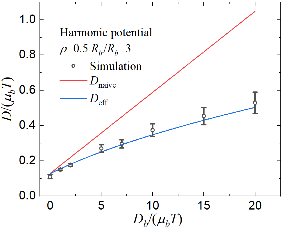
(b)

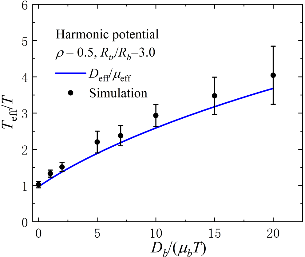
Figure 2: Effective diffusion coefficient with bath activity for different conditions: (a)harmonic potentials and number density of active bath is $\rho=0.5$ , red line shows the linearly dependent of $D_{{\rm naive}}$ on $D_{b}$, and blue line is the effective diffusivity $D_{{\rm eff}}$ with the self-consistent correction. Round circles are simulation data in the same parameters. (b) Effective temperature defined as $T_{{\rm eff}}=D_{{\rm eff}}/\mu_{{\rm eff}}$, the parameters are the same as (a). Simulation details: in this case, we choose $L=50R_{b}$, $\epsilon_{U}:\epsilon_{V}:T=20:100:1$, $\mu_{tr}/\mu_{b}=0.2$, $\tau_{p}=0.5R_{b}^{2}/(\mu_{b}T)$.

IV Conclusion

Motivated by a series of works about tracer in nonequilibrium baths, we presented a theoretical method to investigate the transport properties of the tracer in such environments, including effective diffusion and mobility. The theory begins with the equations of motion for tracer and driven bath particles. Using the procedure of linearized Dean’s equation and the mean-field theory approximation, we derived a generalized Langevin equation for the tracer, wherein a memory kernel and two nontrivial colored noises are involved. To understand the relationships of mobility and diffusivity with the properties of the driven bath, we firstly introduced an adiabatic approximation to calculate these transport coefficients. However, these results are only valid when time-scales of tracer and bath particles are clearly separated. For more general situations, we considered the associated long-time behavior and introduced the Gaussian approximation. As a result, self-consistent equations for effective diffusion and mobility are derived. Numerical calculation shows good conformance with simulation data. We also defined an effective temperature through the quotient of diffusivity and mobility, the theoretical result also agrees with the simulation.

For future works, we wish to study more statistical properties of the system such as linear response and fluctuation theorem. For more in-depth research, we also want to study the relationship between transport properties and the bath properties, such as density, persistent time of particle, or other kinds of active particles. Further we want to reform the system to a Brownian heat engine in active bath. We also notice that the non-Gaussian distribution behavior of a tracer in active baths [40, 11], and hope our theory can bring theoretical understanding about this issue. We may also use this theoretical framework to study multi tracers system and investigate the effective interactions between tracers.

This work is supported by MOST(2018YFA0208702), NSFC (32090044, 21973085, 21833007, 21790350, 21521001), Anhui Initiative in Quantum Information Technologies (AHY090200), and the Fundamental Research Funds for the Central Universities (WK2340000104).

Appendix A Derivation Details

A.1 Derivation of Linearized Dean’s equation

Firstly, we address the one-dimensional model to briefly illustrate the derivation of Eq.(48). The generalization to higher dimensional system is trivial. Consider a stochastic differential equation(SDE), $\frac{{\rm d}x}{{\rm d}t}=a(x,t)+b(x,t)\eta(t)$ where $\left\langle\eta(t)\right\rangle=0$ and $\left\langle\eta(t)\eta(t^{\prime})\right\rangle=\delta(t-t^{\prime})$ denote the Gaussian white noise. Using the It${\rm\hat{o}}$ calculus, for any well behaved function $f(x)$, one has

$$\frac{{\rm d}f(x)}{{\rm d}t}=\left[a(x,t)\partial_{x}f+\frac{b^{2}(x,t)}{2}\partial_{x}^{2}f\right]+\left(\partial_{x}f\right)b(x,t)\eta(t)$$ (44)

Now substituting the Langevin equation (2) of bath particles for the SDE above, using the It${\rm\hat{o}}$ calculus, we have an evolution equation for arbitrary function $g({\bf r}_{i})$

$$\frac{{\rm d}g\left({\bf r}_{i}\right)}{{\rm d}t}= \sqrt{2\mu_{b}T}\boldsymbol{\xi}_{i}\cdot\nabla_{i}g+\left(\nabla_{i}g\right)\left[-\mu_{b}\nabla_{i}\left(\sum_{j\neq i}V+U\right)+{\bf f}_{i}\right]+\mu_{b}T\nabla_{i}^{2}g$$

$$= \int{\rm d}{\bf r}\rho_{i}({\bf r},t)\left\{\sqrt{2\mu_{b}T}\boldsymbol{\xi}_{i}\cdot\nabla g+\left(\nabla g\right)\left[-\mu_{b}\nabla\left(\int{\rm d}{\bf r}^{\prime}\rho({\bf r}^{\prime},t)V\left(\left|{\bf r}-{\bf r}^{\prime}\right|\right)+U\left(\left|{\bf r}-{\bf x}\right|\right)\right)+{\bf f}_{i}\right]+\mu_{b}T\nabla^{2}g\right\}$$

$$= \int{\rm d}{\bf r}g({\bf r})\left\{-\sqrt{2\mu_{b}T}\nabla\rho_{i}\cdot\boldsymbol{\xi}_{i}-\nabla\cdot\left[{\bf f}_{i}\rho_{i}({\bf r},t)\right]+\mu_{b}\nabla\rho_{i}({\bf r},t)\right.$$

$$\cdot\left.\left[\nabla\left(\int{\rm d}{\bf r}^{\prime}\rho({\bf r}^{\prime},t)V\left(\left|{\bf r}-{\bf r}^{\prime}\right|\right)+U\left(\left|{\bf r}-{\bf x}\right|\right)\right)\right]+\mu_{b}T\nabla^{2}\rho_{i}({\bf r},t)\right\}$$ (45)

wherein the bath density $\rho\left({\bf r},t\right)=\sum_{i}\rho_{i}\left({\bf r},t\right)=\sum_{i}\delta\left({\bf r}-{\bf r}_{i}\left(t\right)\right)$ is applied. On the other hand, we can also write $\frac{{\rm d}g({\bf r}_{i})}{{\rm d}t}=\int\frac{\partial\rho_{i}({\bf r},t)}{\partial t}g({\bf r}){\rm d}{\bf r}$. Considering the arbitrariness of function $g({\bf r})$, we have

$$\frac{\partial\rho_{i}\left({\bf r},t\right)}{\partial t}=-\sqrt{2\mu_{b}T}\nabla\rho_{i}\cdot\boldsymbol{\xi}_{i}-\nabla\cdot\left[{\bf f}_{i}\rho_{i}\right]+\mu_{b}\nabla\rho_{i}\cdot\left[\nabla\left(\int{\rm d}{\bf r}^{\prime}\rho({\bf r}^{\prime},t)V\left(\left|{\bf r}-{\bf r}^{\prime}\right|\right)+U\left(\left|{\bf r}-{\bf x}\right|\right)\right)\right]+\mu_{b}T\nabla^{2}\rho_{i}$$ (46)

and the collective density

$$\frac{\partial\rho\left({\bf r},t\right)}{\partial t}=-\sum_{i}\sqrt{2\mu_{b}T}\nabla\cdot\left[\boldsymbol{\xi}_{i}\rho_{i}\right]-\sum_{i}\nabla\cdot\left[{\bf f}_{i}\rho_{i}\right]+\mu_{b}\nabla\rho\cdot\left[\nabla\left(\int{\rm d}{\bf r}^{\prime}\rho({\bf r}^{\prime},t)V\left(\left|{\bf r}-{\bf r}^{\prime}\right|\right)+U\left(\left|{\bf r}-{\bf x}\right|\right)\right)\right]+\mu_{b}T\nabla^{2}\rho$$ (47)

notice that this equation is not closed for the moment, due to the first two noise terms. To achieve Eq.(5), we need to introduce the noise field to replace these terms, meanwhile keeping the correlation properties invariant. Let $\chi_{1}(t)=-\sum_{i}\sqrt{2\mu_{b}T}\nabla\cdot\left[\boldsymbol{\xi}_{i}(t)\rho_{i}({\bf r},t)\right]$, $\chi_{2}(t)=-\sum_{i}\nabla\cdot\left[{\bf f}_{i}(t)\rho_{i}({\bf r},t)\right]$, the time correlation function of these terms are

$$\left\langle\chi_{1}(t)\chi_{1}(t^{\prime})\right\rangle= 2\mu_{b}T\delta(t-t^{\prime})\sum_{i=1}^{N}\nabla_{r}\cdot\nabla_{r^{\prime}}\left[\rho_{i}({\bf r},t)\rho_{i}({\bf r}^{\prime},t^{\prime})\right]$$

$$= 2\mu_{b}T\delta(t-t^{\prime})\nabla_{r}\cdot\nabla_{r^{\prime}}\left[\sum_{i=1}^{N}\rho_{i}({\bf r},t)\delta({\bf r}-{\bf r}^{\prime})\right]$$

$$= 2\mu_{b}T\delta(t-t^{\prime})\nabla_{r}\cdot\nabla_{r^{\prime}}\left[\rho\left({\bf r},t\right)\delta\left({\bf r}-{\bf r}^{\prime}\right)\right]$$

$$\left\langle\chi_{2}(t)\chi_{2}(t^{\prime})\right\rangle= \frac{D_{b}}{\tau_{b}}e^{-\left|t-t^{\prime}\right|/\tau_{b}}\sum_{i=1}^{N}\nabla_{r}\cdot\nabla_{r^{\prime}}\left[\rho_{i}({\bf r},t)\rho_{i}({\bf r}^{\prime},t^{\prime})\right]$$

$$= \frac{D_{b}}{\tau_{b}}e^{-\left|t-t^{\prime}\right|/\tau_{b}}\nabla_{r}\cdot\nabla_{r^{\prime}}\left[\sum_{i=1}^{N}\rho_{i}({\bf r},t)\delta({\bf r}-{\bf r}^{\prime})\right]$$

$$= \frac{D_{b}}{\tau_{b}}e^{-\left|t-t^{\prime}\right|/\tau_{b}}\nabla_{r}\cdot\nabla_{r^{\prime}}\left[\rho\left({\bf r},t\right)\delta\left({\bf r}-{\bf r}^{\prime}\right)\right]$$

Now we introduce two global noise fields, $\chi_{1}^{\prime}\left({\bf r},t\right)=\nabla\cdot\left[\sqrt{\rho\left({\bf r},t\right)}\boldsymbol{\xi}^{T}\right]$ and $\chi_{2}^{\prime}\left({\bf r},t\right)=\nabla\cdot\left[\sqrt{\rho\left({\bf r},t\right)}\boldsymbol{\eta}_{f}\right]$, where the correlations are $\left\langle\boldsymbol{\xi}^{T}\left({\bf r},t\right)\boldsymbol{\xi}^{T}\left({\bf r}^{\prime},t^{\prime}\right)\right\rangle=2\mu_{b}T\delta\left(t-t^{\prime}\right)\delta\left({\bf r}-{\bf r}^{\prime}\right){\bf 1}$ and $\left\langle\boldsymbol{\xi}^{A}\left({\bf r},t\right)\boldsymbol{\xi}^{A}\left({\bf r}^{\prime},t^{\prime}\right)\right\rangle=\frac{D_{b}}{\tau_{b}}\delta\left({\bf r}-{\bf r}^{\prime}\right){\bf 1}$ respectively. It is easy to find out the $\chi_{1}$and $\chi_{1}^{\prime}$ have the same time correlation function, also true for $\chi_{2}$ and $\chi_{2}^{\prime}$. Now we find the replacement and Eq.(47) becomes

$$\frac{\partial\rho\left({\bf r},t\right)}{\partial t}=\nabla\cdot\left[\sqrt{\rho\left({\bf r},t\right)}\boldsymbol{\xi}^{T}\right]+\nabla\cdot\left[\sqrt{\rho\left({\bf r},t\right)}\boldsymbol{\xi}^{A}\right]+\mu_{b}\nabla\rho\cdot\left[\nabla\left(\int{\rm d}{\bf r}^{\prime}\rho({\bf r}^{\prime},t)V\left(\left|{\bf r}-{\bf r}^{\prime}\right|\right)+U\left(\left|{\bf r}-{\bf x}\right|\right)\right)\right]+\mu_{b}T\nabla^{2}\rho$$ (48)

i.e. Eq.(5), which is a self-consistent equation.

Although we use this mean-field approximation to simply the time evolution equation of collective density, this equation is still to hard to solve. For a system that the density fluctuation is small, we can further assume that $\sqrt{\rho\left({\bf r},t\right)}\approx\sqrt{\bar{\rho}}$ where $\bar{\rho}=N/V$ is the averaged number density. This approximation is also used to simplify the interaction terms, $\rho({\bf r})\int{\rm d}{\bf r}^{\prime}\rho({\bf r}^{\prime})\nabla V\left(\left|{\bf r}-{\bf r}^{\prime}\right|\right)\approx\bar{\rho}\rho({\bf r})*\nabla_{r}V({\bf r})$ and $\rho({\bf r})\nabla U\left(\left|{\bf r}-{\bf x}\right|\right)\approx\bar{\rho}\nabla U\left(\left|{\bf r}-{\bf x}\right|\right)$, which is $i{\bf k}e^{i{\bf k}\cdot{\bf x}}\bar{\rho}U_{k}$ in Fourier space. Using the Fourier transform $\delta\rho_{k}(t)=\int e^{i{\bf k}\cdot{\bf r}}\left[\rho\left({\bf r},t\right)-\bar{\rho}\right]{\rm d}{\bf r}$, we have

$$\frac{\partial\delta\rho_{k}\left(t\right)}{\partial t}=-\mu_{b}k^{2}\left[\left(T+\bar{\rho}V_{k}\right)\delta\rho_{k}\left(t\right)+\bar{\rho}U_{k}e^{i{\bf k}\cdot{\bf x}}\right]+\sqrt{\bar{\rho}}i{\bf k}\cdot\left[\tilde{\boldsymbol{\xi}}_{k}^{T}\left(t\right)+\tilde{\boldsymbol{\xi}}_{k}^{A}\left(t\right)\right]$$ (49)

where $V_{k}$ , $U_{k}$, $\tilde{\boldsymbol{\xi}}_{k}^{T}$ and $\tilde{\boldsymbol{\xi}}_{k}^{A}$ are Fourier transforms of $V(r)$, $U(r)$, $\boldsymbol{\xi}^{T}$ and $\boldsymbol{\xi}^{A}$ respectively. This is the Eq.(8) in the main text.

A.2 Derivation of generalized Langevin equation

From equation (11),

$$\mu_{t}\int_{-\infty}^{t}{\bf F}\left({\bf x}\left(t\right)-{\bf x}\left(s\right),t-s\right){\rm d}s$$

$$= -\mu_{t}\mu_{b}\bar{\rho}\int_{-\infty}^{t}{\rm d}s\int_{{\bf k}}i{\bf k}k^{2}U_{k}^{2}e^{-i{\bf k}\cdot\left[{\bf x}\left(t\right)-{\bf x}(s)\right]}e^{-\left(t-s\right)/a_{k}}$$

$$\approx -\frac{\mu_{t}\mu_{b}\bar{\rho}}{d}\int_{-\infty}^{t}{\rm d}s\int_{{\bf k}}k^{4}U_{k}^{2}e^{-\left(t-s\right)/a_{k}}\left[\int_{s}^{t}{\rm d}u\dot{{\bf x}}(u)\right]$$

$$= -\frac{\mu_{t}\mu_{b}\bar{\rho}}{d}\int_{-\infty}^{t}{\rm d}u\int_{-\infty}^{u}{\rm d}s\dot{{\bf x}}(u)\int_{{\bf k}}k^{4}U_{k}^{2}e^{-\left(t-s\right)/a_{k}}$$

$$= -\frac{\mu_{t}\mu_{b}\bar{\rho}}{d}\int_{-\infty}^{t}{\rm d}u\dot{{\bf x}}(u)\int_{{\bf k}}k^{4}U_{k}^{2}a_{k}e^{-\left(t-u\right)/a_{k}}$$ (50)

The approximation is about the term $e^{-i{\bf k}\cdot\left[{\bf x}\left(t\right)-{\bf x}(s)\right]}$. According to the symmetry properties of $U_{k}$ and $a_{k}$ in ${\bf k}$-space, only odd terms of $k$ in $e^{-i{\bf k}\cdot\left[{\bf x}\left(t\right)-{\bf x}(s)\right]}$ contribute to the integral. Using the Taylor expansion and omitting the $O(k^{3})$ terms, we write $e^{-i{\bf k}\cdot\left[{\bf x}\left(t\right)-{\bf x}(s)\right]}\rightarrow-i{\bf k}\cdot\left[{\bf x}\left(t\right)-{\bf x}(s)\right]=-i{\bf k}\cdot\int_{s}^{t}{\rm d}u\dot{{\bf x}}(u)$. With this approximation, and then exchange the order of integrals over $u$ and $s$, we get the finial result.

A.3 Derivation of correlation function of colored noise

Firstly we emphasis that the size of the tracer particle is apparently large than that of the bath particles. This leads to a shorter characteristic time scale for the evolution of the tracer than the bath particles as well. This understanding helps us in the following derivation. The correlations of noise $\boldsymbol{\eta}_{A,T}(t)$ is written as

$$\left\langle\boldsymbol{\eta}_{A,T}\left(t\right)\cdot\boldsymbol{\eta}_{A,T}\left(t^{\prime}\right)\right\rangle$$

$$= \mu_{t}^{2}\bar{\rho}\int_{{\bf k}}\int_{{\bf q}}{\bf k}\cdot{\bf q}U_{k}U_{q}\int_{-\infty}^{t}{\rm d}s\int_{-\infty}^{t^{\prime}}{\rm d}s^{\prime}e^{-\left(t-s\right)/a_{k}-\left(t^{\prime}-s^{\prime}\right)/a_{q}}\left\langle e^{-i{\bf k}\cdot{\bf x}(t)-i{\bf q}\cdot{\bf x}(t^{\prime})}{\bf k}\cdot\tilde{\boldsymbol{\xi}}_{k}^{A,T}(s){\bf q}\cdot\tilde{\boldsymbol{\xi}}_{q}^{A,T}(s^{\prime})\right\rangle$$

$$\approx \mu_{t}^{2}\bar{\rho}\int_{{\bf k}}\int_{{\bf q}}{\bf k}\cdot{\bf q}U_{k}U_{q}\int_{-\infty}^{t}{\rm d}s\int_{-\infty}^{t^{\prime}}{\rm d}s^{\prime}e^{-\left(t-s\right)/a_{k}-\left(t^{\prime}-s^{\prime}\right)/a_{q}}\left\langle e^{-i{\bf k}\cdot{\bf x}(t)-i{\bf q}\cdot{\bf x}(t^{\prime})}\right\rangle\left\langle{\bf k}\cdot\tilde{\boldsymbol{\xi}}_{k}^{A,T}(s){\bf q}\cdot\tilde{\boldsymbol{\xi}}_{q}^{A,T}(s^{\prime})\right\rangle$$ (51)

Herein, the reason why the correlation can be divided into two parts is that ${\bf x}(t)$ can be seen as a slow variable and $\tilde{\boldsymbol{\xi}}_{k}^{A,T}(s)$ are fast variables, i.e. there is a time scale separation between ${\bf x}(t)$ and $\tilde{\boldsymbol{\xi}}_{k}^{A,T}(s)$. At the typical time scale of ${\bf x}(t)$ evolution, noise $\tilde{\boldsymbol{\xi}}_{k}^{A,T}(s)$ has been sufficiently averaged, which is zero. Finally we have the form above.

Notice that the Fourier transform of a white noise herein is actually firstly calculating the correlation and then proceeding the transform. Therefore,

$$\left\langle{\bf k}\cdot\tilde{\boldsymbol{\xi}}_{k}^{T}(s){\bf q}\cdot\tilde{\boldsymbol{\xi}}_{q}^{T}(s^{\prime})\right\rangle$$

$$= {\bf k}\cdot\iint{\rm d}{\bf r}{\rm d}{\bf r}^{\prime}e^{i{\bf k}\cdot{\bf r}}e^{i{\bf q}\cdot{\bf r}^{\prime}}\left\langle\boldsymbol{\xi}^{T}({\bf r},s)\boldsymbol{\xi}^{T}({\bf r}^{\prime},s^{\prime})\right\rangle\cdot{\bf q}$$

$$= 2\mu_{b}T\delta(s-s^{\prime})(2\pi)^{d}\delta({\bf k}+{\bf q}){\bf k}\cdot{\bf I}\cdot{\bf q}$$

$$= -2\mu_{b}Tk^{2}\delta(s-s^{\prime})(2\pi)^{d}\delta({\bf k}+{\bf q})$$ (52)

this demands ${\bf k}=-{\bf q}$. Similarly, we also have

$$\left\langle{\bf k}\cdot\tilde{\boldsymbol{\xi}}_{k}^{A}(s){\bf q}\cdot\tilde{\boldsymbol{\xi}}_{q}^{A}(s^{\prime})\right\rangle=\frac{D_{b}}{\tau_{b}}e^{-|s-s^{\prime}|/\tau_{b}}k^{2}(2\pi)^{d}\delta({\bf k}+{\bf q})$$ (53)

Bringing these into Eq.(51), we have Eqs.(21) and (20) in the main text.

References

- [1] Xiao-Lun Wu and Albert Libchaber. Particle diffusion in a quasi-two-dimensional bacterial bath. Physical Review Letters, 84(13):3017, 2000.
- [2] U. Seifert and T. Speck. Fluctuation-dissipation theorem in nonequilibrium steady states. EPL (Europhysics Letters), 89(1):10007, 2010.
- [3] Christian Maes and Stefano Steffenoni. Friction and noise for a probe in a nonequilibrium fluid. Phys. Rev. E, 91:022128, Feb 2015.
- [4] Clemens Bechinger, Roberto Di Leonardo, Hartmut Löwen, Charles Reichhardt, Giorgio Volpe, and Giovanni Volpe. Active particles in complex and crowded environments. Reviews of Modern Physics, 88(4):045006, 2016.
- [5] Johannes Berner, Boris Müller, Juan Ruben Gomez-Solano, Matthias Krüger, and Clemens Bechinger. Oscillating modes of driven colloids in overdamped systems. Nature Communications, 9(1):999, 2018.
- [6] Eric W. Burkholder and John F. Brady. Fluctuation-dissipation in active matter. The Journal of Chemical Physics, 150(18):184901, 2019.
- [7] Peng Liu, Simin Ye, Fangfu Ye, Ke Chen, and Mingcheng Yang. Constraint dependence of active depletion forces on passive particles. Phys. Rev. Lett., 124:158001, Apr 2020.
- [8] Daniel TN Chen, AWC Lau, Lawrence A Hough, Mohammad F Islam, Mark Goulian, Thomas C Lubensky, and Arjun G Yodh. Fluctuations and rheology in active bacterial suspensions. Physical Review Letters, 99(14):148302, 2007.
- [9] L. Angelani, C. Maggi, M. L. Bernardini, A. Rizzo, and R. Di Leonardo. Effective interactions between colloidal particles suspended in a bath of swimming cells. Phys. Rev. Lett., 107:138302, Sep 2011.
- [10] Claudio Maggi, Matteo Paoluzzi, Nicola Pellicciotta, Alessia Lepore, Luca Angelani, and Roberto Di Leonardo. Generalized energy equipartition in harmonic oscillators driven by active baths. Physical review letters, 113(23):238303, 2014.
- [11] Claudio Maggi, Matteo Paoluzzi, Luca Angelani, and Roberto Di Leonardo. Memory-less response and violation of the fluctuation-dissipation theorem in colloids suspended in an active bath. Scientific reports, 7(1):17588, 2017.
- [12] G. M. Wang, E. M. Sevick, Emil Mittag, Debra J. Searles, and Denis J. Evans. Experimental demonstration of violations of the second law of thermodynamics for small systems and short time scales. Phys. Rev. Lett., 89:050601, Jul 2002.
- [13] J. Harder, C. Valeriani, and A. Cacciuto. Activity-induced collapse and reexpansion of rigid polymers. Phys. Rev. E, 90:062312, Dec 2014.
- [14] N Koumakis, A Lepore, C Maggi, and R Di Leonardo. Targeted delivery of colloids by swimming bacteria. Nature communications, 4(1):1–6, 2013.
- [15] Markus Rauscher, Alvaro Domínguez, Matthias Krüger, and Florencia Penna. A dynamic density functional theory for particles in a flowing solvent. The Journal of Chemical Physics, 127(24):244906, 2007.
- [16] Marco Baiesi, Christian Maes, and Bram Wynants. Fluctuations and response of nonequilibrium states. Phys. Rev. Lett., 103:010602, Jul 2009.
- [17] Vincent Démery and David S. Dean. Perturbative path-integral study of active- and passive-tracer diffusion in fluctuating fields. Phys. Rev. E, 84:011148, Jul 2011.
- [18] Juan Ruben Gomez-Solano, Artyom Petrosyan, Sergio Ciliberto, and Christian Maes. Fluctuations and response in a non-equilibrium micron-sized system. Journal of Statistical Mechanics: Theory and Experiment, 2011(01):P01008, jan 2011.
- [19] C. Maes, S. Safaverdi, P. Visco, and F. van Wijland. Fluctuation-response relations for nonequilibrium diffusions with memory. Phys. Rev. E, 87:022125, Feb 2013.
- [20] Vincent Démery, Olivier Bénichou, and Hugo Jacquin. Generalized langevin equations for a driven tracer in dense soft colloids: construction and applications. New Journal of Physics, 16(5):053032, may 2014.
- [21] Grzegorz Szamel. Self-propelled particle in an external potential: Existence of an effective temperature. Physical Review E, 90(1):012111, 2014.
- [22] Matthias Krüger and Christian Maes. The modified langevin description for probes in a nonlinear medium. Journal of Physics: Condensed Matter, 29(6):064004, dec 2016.
- [23] Eric W Burkholder and John F Brady. Tracer diffusion in active suspensions. Physical Review E, 95(5):052605, 2017.
- [24] Christian Maes. Fluctuating motion in an active environment. Phys. Rev. Lett., 125:208001, Nov 2020.
- [25] Christian Maes. Response theory: A trajectory-based approach. Frontiers in Physics, 8:229, 2020.
- [26] Vincent Démery and Étienne Fodor. Driven probe under harmonic confinement in a colloidal bath. Journal of Statistical Mechanics: Theory and Experiment, 2019(3):033202, mar 2019.
- [27] Olivier Dauchot and Vincent Démery. Dynamics of a self-propelled particle in a harmonic trap. Phys. Rev. Lett., 122:068002, Feb 2019.
- [28] Vincent Démery and David S. Dean. Drag forces in classical fields. Phys. Rev. Lett., 104:080601, Feb 2010.
- [29] I. Gazuz, A. M. Puertas, Th. Voigtmann, and M. Fuchs. Active and nonlinear microrheology in dense colloidal suspensions. Phys. Rev. Lett., 102:248302, Jun 2009.
- [30] I. Gazuz and M. Fuchs. Nonlinear microrheology of dense colloidal suspensions: A mode-coupling theory. Phys. Rev. E, 87:032304, Mar 2013.
- [31] B. Lander, U. Seifert, and T. Speck. Mobility and diffusion of a tagged particle in a driven colloidal suspension. EPL (Europhysics Letters), 92(5):58001, 2011.
- [32] David S Dean and Vincent Démery. Diffusion of active tracers in fluctuating fields. Journal of Physics: Condensed Matter, 23(23):234114, may 2011.
- [33] L. L. Bonilla. Active ornstein-uhlenbeck particles. Phys. Rev. E, 100:022601, Aug 2019.
- [34] Michael E. Cates and Julien Tailleur. Motility-induced phase separation. Annual Review of Condensed Matter Physics, 6(1):219–244, 2015.
- [35] Gerhard Gompper, Roland G Winkler, Thomas Speck, Alexandre Solon, Cesare Nardini, Fernando Peruani, Hartmut Löwen, Ramin Golestanian, U Benjamin Kaupp, Luis Alvarez, et al. The 2020 motile active matter roadmap. Journal of Physics: Condensed Matter, 32(19):193001, 2020.
- [36] David S Dean. Langevin equation for the density of a system of interacting langevin processes. Journal of Physics A: Mathematical and General, 29(24):L613–L617, dec 1996.
- [37] David Chandler. Introduction to modern statistical mechanics, volume 40. Oxford University Press, Oxford, UK, 1987.
- [38] Min Jun Kim and Kenneth S Breuer. Enhanced diffusion due to motile bacteria. Physics of fluids, 16(9):L78–L81, 2004.
- [39] Claudio Maggi, Umberto Marini Bettolo Marconi, Nicoletta Gnan, and Roberto Di Leonardo. Multidimensional stationary probability distribution for interacting active particles. Scientific reports, 5, 2015.
- [40] Kyriacos C Leptos, Jeffrey S Guasto, Jerry P Gollub, Adriana I Pesci, and Raymond E Goldstein. Dynamics of enhanced tracer diffusion in suspensions of swimming eukaryotic microorganisms. Physical Review Letters, 103(19):198103, 2009.