SALSA: Spatial Cue-Augmented
Log-Spectrogram Features for Polyphonic
Sound Event Localization and Detection

Abstract

Sound event localization and detection (SELD) consists of two subtasks, which are sound event detection and direction-of-arrival estimation. While sound event detection mainly relies on time-frequency patterns to distinguish different sound classes, direction-of-arrival estimation uses amplitude and/or phase differences between microphones to estimate source directions. As a result, it is often difficult to jointly optimize these two subtasks. We propose a novel feature called Spatial cue-Augmented Log-SpectrogrAm (SALSA) with exact time-frequency mapping between the signal power and the source directional cues, which is crucial for resolving overlapping sound sources. The SALSA feature consists of multichannel log-spectrograms stacked along with the normalized principal eigenvector of the spatial covariance matrix at each corresponding time-frequency bin. Depending on the microphone array format, the principal eigenvector can be normalized differently to extract amplitude and/or phase differences between the microphones. As a result, SALSA features are applicable for different microphone array formats such as first-order ambisonics (FOA) and multichannel microphone array (MIC). Experimental results on the TAU-NIGENS Spatial Sound Events 2021 dataset with directional interferences showed that SALSA features outperformed other state-of-the-art features. Specifically, the use of SALSA features in the FOA format increased the F1 score and localization recall by $6\text{\,}\mathrm{\char 37\relax}$ each, compared to the multichannel log-mel spectrograms with intensity vectors. For the MIC format, using SALSA features increased F1 score and localization recall by $16\text{\,}\mathrm{\char 37\relax}$ and $7\text{\,}\mathrm{\char 37\relax}$, respectively, compared to using multichannel log-mel spectrograms with generalized cross-correlation spectra.

I Introduction

Sound event localization and detection (SELD) has many applications in urban sound sensing [1], wildlife monitoring [2], surveillance [3], autonomous driving, and robotics [4]. SELD is an emerging research field that unifies the tasks of sound event detection (SED) and direction-of-arrival estimation (DOAE) by jointly recognizing the sound classes, and estimating the directions of arrival (DOA), the onsets, and the offsets of detected sound events [5]. Because of a need for source localization, SELD typically requires multichannel audio inputs from a microphone array, which has several formats in current use, such as first-order ambisonics (FOA) and multichannel microphone array (MIC).

I-A Existing methods

TABLE I: Comparison of the proposed method with some existing deep learning-based methods for polyphonic SELD.

Approach		Format	Input Features	Network Architecture	Output
Adavanne et al.	[5]	FOA/MIC	Magnitude & phase spectrograms	End-to-end CRNN	class-wise
Cao et al.	[7]	FOA/MIC	Log-mel spectrograms, GCC-PHAT	Two-stage CRNNs	class-wise
Nguyen et al.	[9]	FOA	Log-mel spectrograms, directional SS histograms	Sequence matching CRNN	track-wise
Xue et al.	[Xue2020SoundLearning]	MIC	Log-mel spectrograms, IV, pair-wise phase differences	Modified two-stage CRNNs	class-wise
Cao et al.	[12]	FOA	Log-mel spectrograms, IV	EINv2	track-wise
Shimada et al.	[Shimada2021ACCDOA:Detection]	FOA	Linear amplitude spectrograms, IPD	CRNN with D3Net	class-wise
Sato et al.	[13]	FOA	Complex spectrograms	Invariant CRNN	class-wise
Phan et al.	[14]	FOA/MIC	Log-mel spectrograms, IV, GCC-PHAT	CRNN with self attention	class-wise
Park et al.	[Park2020SoundFunctions]	FOA	Log-mel spectrograms, IV, harmonic percussive separation	CRNN with feature pyramid	class-wise
Emmanuel et al.	[Emmanuel2021Multi-scaleDetection]	FOA	Constant-Q spectrograms, log-mel spectrograms, IV	Multi-scale network with MHSA	track-wise
Lee et al.	[Lee2021SoundChallenge]	FOA	Log-mel spectrograms, IV	EINv2 with cross-model attention	track-wise
(Top’19) Kapka et al.	[Kapka2019SoundModels]	FOA	Log-mel spectrograms, IV	Ensemble of CRNNs	class-wise
(Top’20) Wang et al.	[Wang2020TheChallenge]	FOA+MIC	Log-mel spectrograms, IV, GCC-PHAT	Ensemble of CRNNs & CNN-TDNNs	class-wise
(Top’21) Shimada et al.	[Shimada2021EnsembleDetection]	FOA	Linear amplitude spectrograms, IPD, cosIPD, sinIPD	Ensemble of CRNNs & EINv2	class-wise
Proposed method		FOA/MIC	SALSA: Log-linear spectrograms & normalized eigenvectors	End-to-end CRNN	class-wise

IV and GCC-PHAT features follow the frequency scale (linear, mel, constant-Q) of the spectrograms. TDNN stands for time delay neural networks. IPD stands for interchannel phase differences. Top’YY denotes the top ranked systems for the respective DCASE SELD Challenges.

Over the past few years, there have been many major developments for SELD in the areas of data augmentation, feature engineering, model architectures, and output formats. In 2015, an early monophonic SELD work by Hirvonen [6] formulated SELD as a classification task. In 2018, Adavanne et al. [5] pioneered a seminal polyphonic SELD work that used an end-to-end convolutional recurrent neural network (CRNN), SELDnet, to jointly detect sound events and estimate the corresponding DOAs. In 2019, SELD task was introduced in the Challenge on Detection and Classification of Acoustic Scenes and Events (DCASE). Cao et al. [7] proposed a two-stage strategy by training separate SED and DOAE models. Mazzon et al. [8] proposed a spatial augmentation method by swapping channels of FOA format. Nguyen et al. [9, 10] explored a hybrid approach called a Sequence Matching Network (SMN) that matched the SED and DOAE output sequences using a bidirectional gated recurrent unit (BiGRU).

In 2020, moving sound sources were introduced in the DCASE SELD Challenge. Cao et al. [11] proposed Event Independent Network (EIN) that used soft parameter sharing between the SED and DOAE encoder branches and output track-wise predictions. An improved version of this network, EINv2, replaced the biGRUs with multi-head self-attention (MHSA) [12]. Sato et al. [13] designed a CRNN that is invariant to rotation, scale, and time translation for FOA signals. Phan et al. [14] formulated SELD as regression problems for both SED and DOAE to improve training convergence. Wang et al. [15] focused on several data augmentation methods to overcome the data sparsity problem in SELD. Shimada et al. [Shimada2021ACCDOA:Detection] unified SED and DOAE losses into one regression loss using a representation technique called Activity-Coupled Cartesian Direction of Arrival (ACCDOA). In 2021, unknown interferences were introduced in the DCASE SELD challenge. Lee et al. [Lee2021SoundChallenge] enhanced EINv2 by adding cross-modal attention between the SED and DOAE branches. Table I summarizes some notable and state-of-the-art deep learning methods for SELD.

I-B Input features for SELD

In this paper, we focus on input features for SELD. When SELDnet was first introduced, it was trained on multichannel magnitude and phase spectrograms [5]. Subsequently, different features, such as multichannel log-spectrograms and intensity vector (IV) for the FOA format, and generalized cross-correlation with phase transform (GCC-PHAT) for the MIC format in the mel scale were shown to be more effective for SELD [Politis2020ADetection, Politis2021, 7, 12, Shimada2021ACCDOA:Detection, 15, Wang2020TheChallenge, Shimada2021EnsembleDetection].

Due to the smaller dimension size and stronger emphasis on the lower frequency bands, where signal contents are mostly populated, the mel frequency scale has been used more frequently than the linear frequency scale for SELD. However, combining the IV or GCC-PHAT features with the mel spectrograms is not trivial and the implicit DOA information stored in the former features are often compromised. In practice, the IVs are also passed through the mel filters which merge DOA cues in different narrow bands into one mel band, making it more difficult to resolve different DOAs in multi-source scenarios. Likewise, in order to stack the GCC-PHAT with the mel spectrograms, longer time-lags on the GCC-PHAT have to be truncated. Since the linear scale has the advantage of preserving the directional information at each frequency band, several works have attempted to use spectrogram, inter-channel phase differences (IPD), and IVs in linear scale [Shimada2021ACCDOA:Detection] or the constant-Q scale [Emmanuel2021Multi-scaleDetection]. However, there is lack of experimental results that directly compare these features over different scales.

Referring to Table I, more SELD algorithms have been developed for the FOA format compared to the MIC format, even though the MIC format is more common in practice. The baselines for three DCASE SELD challenges so far have indicated that using FOA inputs performs slightly better than that with MIC inputs [Adavanne2019ADetection, Politis2020ADetection, Politis2021]. In addition, it is more straightforward to stack IVs with the spectrograms in the FOA format compared to stacking GCC-PHAT with spectrograms. When IVs are stacked with spectrograms, there is a direct frequency correspondence between the IVs and the spectrograms. This frequency correspondence is crucial for networks to associate the sound classes and the DOAs of multiple sound events, where signals of different sound sources are often distributed differently along the frequency dimension. On the other hand, the time-lag dimension of the GCC-PHAT features does not have a local linear one-to-one mapping with the frequency dimension of the spectrograms. As a result, all of the DOA information is aggregated at the frame level, making it difficult to assign correct DOAs to different sound events. Furthermore, when there are multiple sound sources, GCC-PHAT features are known to be noisy, and the directional cues at overlapping TF bins of IVs are merged. In order to solve SELD more effectively in noisy, reverberant, and multi-source scenarios, a better feature is needed for both audio formats, but especially for the MIC format where feature engineering has largely been lacking compared to the FOA format.

I-C Our Contributions

We propose a novel feature for SELD called Spatial Cue-Augmented Log-Spectrogram (SALSA) with exact spectrotemporal mapping between the signal power and the source DOA for both FOA and MIC formats. The feature consists of multichannel log-magnitude linear-frequency spectrograms stacked with a normalized version of the principal eigenvector of the spatial covariance matrix at each TF bin on the spectrograms. The principal eigenvector is normalized such that it represents the inter-channel intensity difference (IID) for the FOA format, and/or inter-channel phase difference (IPD) for the MIC format.

To further improve the performance, only eigenvectors from approximately single-source TF bins are included in the features since these directional cues are less noisy. A TF bin is considered a single-source bin when it contains energy mostly from only one source [Nguyen2014RobustSources, Nguyen2020RobustNetwork]. We evaluated the effectiveness of the proposed feature on both the FOA and the MIC formats using the TAU-NIGENS Spatial Sound Events (TNSSE) 2021 dataset used in DCASE 2021 SELD Challenge. Experimental results showed that the SALSA feature outperformed, for the FOA format, both mel- and linear-frequency log-magnitude spectrograms with IV, and for the MIC format, the log-magnitude spectrogram with GCC-PHAT.

In addition, SALSA features bridged the performance gap between the FOA and the MIC formats, and achieved the state-of-the-art performance for a single (non-ensemble) model on the TNSSE 2021 development dataset for both formats. Similarly, when evaluated on the TNSSE 2020 dataset, SALSA also achieved the top performance for a single model for both formats on both the development and the evaluation datasets. Our ensemble model trained on an early version of SALSA features ranked second in the team category of the DCASE 2021 SELD challenge [Nguyen2021DCASEDetection].

Our paper offers several contributions, as follows:

1. a novel and effective feature for SELD that works for both FOA and MIC formats,

2. an improvement to the proposed feature by utilizing signal processing-based methods to select single-source TF bins,

3. a comprehensive analysis of feature importance of each components in SALSA for SELD, and,

4. an extensive ablation study of different data augmentation methods for the newly proposed SALSA feature, as well as for the log-magnitude spectrograms with IV and GCC-PHAT in both linear- and mel-frequency scales.

The rest of the paper is organized as follows. Section II presents the proposed SALSA features for both the FOA and the MIC formats. Section III briefly describes common SELD features used as benchmarks. Section IV presents the network architecture employed in all of the experiments. Section V elaborates the experimental settings. Section VI presents the experimental results and discussion with extensive ablation study. Finally, we conclude the paper in Section VII. The source code for reproducing our work can be found at https://github.com/thomeou/SALSA.

II Spatial Cue-Augmented Log-Spectrogram Features for SELD

The proposed SALSA features consist of two major components: multichannel log-linear spectrograms and normalized principal eigenvectors. For the rest of this paper, spectrograms refer to multichannel spectrograms unless otherwise stated.

II-A Signal Model

Let $M$ be the number of microphones and $L$ be the number of sound sources. The short-time Fourier transform (STFT) signal observed by an $M$-channel microphone array of arbitrary geometry in the TF domain is given by

$$\mathbf{X}(t,f)=\sum_{i=1}^{L}S_{i}(t,f)\mathbf{H}(f,\phi_{i},\theta_{i})+\mathbf{V}(t,f)\in\mathbb{C}^{M},$$ (1)

where $t$ and $f$ are time and frequency indices, respectively; $S_{i}$ is the $i$th source signal; $\mathbf{H}(f,\phi_{i},\theta_{i})$ is the frequency-domain steering vector corresponding to the DOA ($\phi_{i},\theta_{i}$) of the $i$th source, where $\phi_{i}$ and $\theta_{i}$ are the azimuth and elevation angles, respectively; and $\mathbf{V}$ is the noise vector. For moving sources, $\phi_{i}=\phi_{i}(t)$ and $\theta_{i}=\theta_{i}(t)$ are functions of time. For brevity, the time variable is omitted in $\phi_{i}$ and $\theta_{i}$ for some equations. Note that Eq. 1 is applicable for TF bins that have relatively low reverberation, which can be absorbed into the $\mathbf{V}$ term. TF bins with relative high direct-to-reverberant energy ratios would be preferably excluded from the estimation in this work.

II-B Multichannel log-linear spectrograms

The log-linear spectrograms are computed from the complex spectrograms $\mathbf{X}(t,f)$ by

$$\textsc{LinSpec}(t,f)=\log\left(\left\lvert\mathbf{X}(t,f)\right\rvert^{2}\right)\in\mathbb{R}^{M\times T\times F},$$ (2)

where $\lvert\cdot\rvert$, is the elementwise complex modulus, $T$ is the number of time frames and $F$ is the number of frequency bins.

II-C Normalized principal eigenvectors

Assuming the signal and noise are zero-mean and uncorrelated, the true covariance matrix, $\mathbf{R}(t,f)\in\mathbb{C}^{M\times M}$, is a linear combination of rank-one outer products of the steering vectors weighted by signal powers $\sigma_{i}^{2}(t,f)$ of the $i$th source at the TF bin $(t,f)$, that is,

$$\mathbf{R}(t,f)=\mathbb{E}[\mathbf{X}(t,f)\mathbf{X}^{\mathsf{H}}(t,f)]$$ (3)

$$=\sum_{i=1}^{L}\sigma_{i}^{2}(t,f)\mathbf{H}(f,\phi_{i},\theta_{i})\mathbf{H}^{\mathsf{H}}(f,\phi_{i},\theta_{i})+\mathbf{R}_{\text{n}}(t,f),$$ (4)

where $\mathbf{R}_{\text{n}}(t,f)$ is the noise covariance matrix, and $(\cdot)^{\mathbf{\mathsf{H}}}$ denotes the Hermitian transpose. Note that although the reverberation is also absorbed into the noise vector, the uncorrelated noise assumption can generally hold if the reverberation level is sufficiently low.

In practice, under the assumption that the sources are slow-moving within a small time window, Eq. 3 can be approximated using

$$\mathbf{\hat{R}}(t,f)=\frac{1}{2T_{\text{r}}+1}\sum_{\tau=-T_{\text{r}}}^{T_{\text{r}}}\mathbf{X}(t+\tau,f)\mathbf{X}^{\mathsf{H}}(t+\tau,f)$$ (5)

where $2T_{\text{r}}+1$ is the window size. In this work, we use $T_{\text{r}}=3$.

Eq. 4 shows that at single-source TF bins, where only one sound source is dominant over other sources and reverberation, the theoretical steering vector $\mathbf{H}(f,\phi,\theta)$ can be approximated by the principal eigenvector $\mathbf{U}(t,f)$ of the covariance matrix, a technique previously utilized in multichannel speech separation [Asano2007DetectionArray], as well as in our previous works [Nguyen2014RobustSources, Nguyen2020RobustNetwork]. Therefore, we can reliably extract directional cues from these principal eigenvectors at these bins. For TF bins which are not single-source, the values of the directional cues can be set to a predefined default value such as zero. In the next sections, we elaborate on how to normalize the principal eigenvectors to extract directional cues, which are encoded in the IID and IPD for FOA arrays and far-field microphone arrays, respectively.

II-C1 Eigenvector-based intensity vector for FOA arrays

FOA arrays have four channels and the directional cues are encoded in the IID. A typical steering vector for an FOA array can be defined by

$$\mathbf{H}^{\text{FOA}}(t,\phi,\theta)=\begin{bmatrix}H_{\text{W}}(t,\phi,\theta)\\ H_{\text{X}}(t,\phi,\theta)\\ H_{\text{Y}}(t,\phi,\theta)\\ H_{\text{Z}}(t,\phi,\theta)\end{bmatrix}=\begin{bmatrix}1\\ \cos(\phi)\cos(\theta)\\ \sin(\phi)\cos(\theta)\\ \sin(\theta)\end{bmatrix}\in\mathbb{R}^{4},$$ (6)

where $\phi=\phi(t)$ and $\theta=\theta(t)$ are the time-dependent azimuth and elevation angles of a sound source with respect to the array, respectively.

We can compute an eigenvector-based intensity vector (EIV) to approximate $[H_{\text{X}},H_{\text{Y}},H_{\text{Z}}]^{\mathsf{T}}$ from the principle eigenvector ${\mathbf{U}=\mathbf{U}(t,f)}$ as follows. First, we normalize $\mathbf{U}$ by its first element, which corresponds to the omni-directional channel, then discard the first element to obtain $\mathbf{\bar{U}}$. Afterwards, we take the real part of $\mathbf{\bar{U}}$ and normalize it to obtain unit-norm EIV $\mathbf{\widetilde{U}}=\Re(\mathbf{\bar{U}})/\|\Re(\mathbf{\bar{U}})\|$. SALSA features for the FOA format are formed by stacking the four-channel spectrograms with the three-channel EIV $\mathbf{\widetilde{U}}$.

Fig. 1 illustrates SALSA features of a $16$-second audio segment in multi-source cases for an FOA array with an EIV cutoff frequency of $9\text{\,}\mathrm{kHz}$. The three EIV channels are visually discriminant for different sources originating from different directions. The green areas in the EIV channels correspond to zeroed-out TF bins. Moreover, due to the spectrotemporal alignment properties of SALSA, it can be observed that the TF patterns of the sources in the spectrogram channels, and the patterns of the corresponding directional cues share similar activation patterns, facilitating multichannel feature extraction that is also spectrotemporally meaningful when used as an input to convolutional layers.

II-C2 Eigenvector-based phase vector for microphone arrays

Figure 1: SALSA features of a 16-second audio segment of FOA format in a multi-source scenario. The vertical axis represents frequency in kHz. In the spectrogram channels, the colormap represents the signal log-magnitude in each TF bin. In the EIV channels, the colormap represents the values of the computed EIV features.

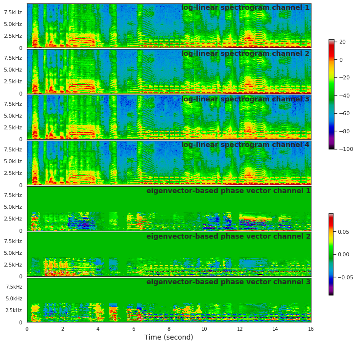
Figure 2: SALSA features of a 16-second audio segment of a four-channel microphone array (MIC format) in a multi-source scenario. The vertical axis represents frequency in kHz. In the spectrogram channels, the colormap represents the signal log-magnitude in each TF bin. In the EPV channels, the colormap represents the values of the computed EPV features.

For a far-field microphone array, the directional cues are encoded in the IPD. The steering vector of an $M$-channel far-field array of an arbitrary geometry can be modelled by $\mathbf{H}^{\text{MIC}}(t,f,\phi,\theta)\in\mathbb{C}^{M}$, whose elements are given by

$$H_{m}^{\text{MIC}}(t,f,\phi,\theta)=\exp\left(-\jmath 2\pi fd_{1m}(\phi(t),\theta(t))/c\right),$$ (7)

where $\jmath$ is the imaginary unit, $c\approx$343\text{\,}\mathrm{m}\text{\,}{\mathrm{s}}^{-1}$$ is the speed of sound; $d_{1m}(\phi(t),\theta(t))$ is the distance of arrival, in metres, travelled by a sound source, between the $m$th microphone and the reference ($m=1$) microphone. In theory, the distance of arrival is given by

$$d_{1m}(\phi(t),\theta(t))=(\bm{\zeta}_{1}-\bm{\zeta}_{m})^{\mathsf{T}}\begin{bmatrix}\cos(\phi(t))\cos(\theta(t))\\ \sin(\phi(t))\cos(\theta(t))\\ \sin(\theta(t))\end{bmatrix}\in\mathbb{R},$$ (8)

where $\bm{\zeta}_{1}$ and $\bm{\zeta}_{m}$ are the Cartesian coordinates of the reference and the $m$th microphones, respectively. $\tau_{1m}(\phi(t),\theta(t))=d_{1m}(\phi(t),\theta(t))/c$ is the time difference of arrival (TDOA), travelled by the sound source, between the $m$th and the reference microphones.

The directional cues of a far-field microphone array can be presented in several forms such as the relative distance of arrival (RDOA) and TDOA. In this study, we choose to extract the directional cues in the form of RDOA. One advantage of RDOA is that we do not need to know the exact coordinates of the individual microphones, since spatial information of the microphones are already implicitly encoded in the RDOA. We can compute an eigenvector-based phase vector (EPV) to approximate $[d_{12},\ldots,d_{1M}]^{T}$ from the principle eigenvector $\mathbf{U}$ as follows. First we normalize $\mathbf{U}$ by its first element, which is chosen arbitrarily as the reference microphone, then discard the first element to obtain $\mathbf{\bar{U}}$. After that, we take the phase of $\mathbf{\bar{U}}$ and normalize it by $-2\pi f/c$ to obtain the EPV $\mathbf{\widetilde{U}}=-c\angle\mathbf{\bar{U}}/(2\pi f)$. The SALSA features for far-field microphone arrays are formed by stacking the $M$-channel spectrograms with the $(M-1)$-channel EPV. To avoid spatial aliasing, the values of $\mathbf{\widetilde{U}}$ are set to zero for all TF bins above aliasing frequency.

Fig. 2 illustrates the SALSA feature of a $16$-second audio segment in multi-source cases for a four-channel microphone array with an EPV cutoff frequency of $4\text{\,}\mathrm{kHz}$. Similar to the FOA counterpart, the three EPV channels are visually discriminant for different sources originating from different directions. The directional cues in the EPV channels also similarly display patterns corresponding to the sources. The green areas in the EPV channels corresponds to zeroed-out TF bins that are not single-source or above aliasing frequency.

The proposed method to extract spatial cues can also be extended to near-field and baffled microphone arrays, where directional cues are encoded in both IID and IPD. For those arrays, we can approximate their array response model using the far-field model, or we can compute both EIV and EPV as shown in Section II-C1 and Section II-C2, respectively.

II-D Single-source time-frequency bin selection

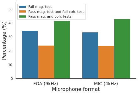
Figure 3: Distributions of TF bins that (a) fail magnitude test, (b) pass magnitude test but fail coherence test, and (c) pass both tests, for the FOA and MIC formats. The distributions shown are independent of the true number of sources.

The selection of single-source TF bins have been shown to be effective for DOAE in noisy, reverberant and multi-source cases [Nguyen2014RobustSources, 9, Nguyen2020RobustNetwork]. There are several methods to select single-source TF bins [Mohan2008LocalizationTest, Pavlidi2013Real-TimeArray, Nguyen2014RobustSources]. In this paper, we apply two tests to select single-source TF bins, namely, the magnitude and coherence tests. The magnitude test aims to select only TF bins that contain signal from foreground sound sources [Nguyen2014RobustSources]. A TF bin passes the magnitude test if its signal-to-noise ratio (SNR) with respect to the adaptive noise floor $\eta[t,f]$ is above a threshold $\alpha_{\text{SNR}}$ [Nguyen2014RobustSources]. In practice, the magnitude test indicator is given by

$$\textsc{MagTest}[t,f]=\mathbb{I}\left[\widetilde{X}_{1}[t,f]>\alpha_{\text{SNR}}\cdot\eta[t,f]\right]\in\{0,1\},$$ (9)

where $\mathbb{I}\left[\cdot\right]$ is the Iverson bracket, and $\widetilde{X}_{1}[t,f]$ is a running root-mean-square of the magnitude of $X_{1}[t,f]$ over a 3-frame window. We set the threshold $\alpha_{\text{SNR}}=1.5$ based on past experiments across several DOAE [Nguyen2014RobustSources, Nguyen2020RobustNetwork, Zhao2015RobustReduction], and SELD [9, Nguyen2020EnsembleTracking, Nguyen2019DCASEDetection] tasks. We used a fast and simple method to estimate the frequency-wise noise floor $\eta[t,f]$ as follows [Nguyen2014RobustSources]. The noise floor is initialized using the first few audio frames, which are assumed to contain only noise. After that, the noise floor is slightly increased or decreased if the magnitude of $X_{1}[t,f]$ is above or below the previous noise floor, respectively. The noise floor can also be computed using other estimators such as the one proposed in [Gerkmann2012UnbiasedDelay].

The coherence test aims to find TF bins that contain signal from mostly one source [Mohan2008LocalizationTest]. Specifically, consider an eigendecomposition, which in practice can be equivalently performed by the more numerically stable SVD,

$$\mathbf{R}(t,f)=\mathbf{U}(t,f)\mathbf{\Sigma}(t,f)\mathbf{U}^{\mathsf{H}}(t,f)$$ (10)

where $\mathbf{\Sigma}(t,f)=\operatorname{diag}\left([\sigma_{1}(t,f),\sigma_{2}(t,f),\cdots,\sigma_{M}(t,f)]\right)$, and $\sigma_{1}(t,f)\geq\sigma_{2}(t,f)\geq\dots\geq\sigma_{M}(t,f)$. The direct-to-reverberant ratio (DRR) is given by

$$\rho(t,f)=\dfrac{\sigma_{1}(t,f)}{\sigma_{2}(t,f)}.$$ (11)

Since the DRR can be interpreted as the relative strength between the paths of signals arriving at the microphone array, the DRR can be also interpreted as a measure of source dominance. When the DRR is low, it is likely that there are either multiple dominant sources at the TF bin, or the reverberation is high even if there is only one source. A TF bin passes the coherence test if its DRR is above a coherence threshold $\beta_{\text{DRR}}$ [Rafaely2017SpeakerStatistics]. In this work, we used $\beta_{\text{DRR}}=5$ which obtained the best performance on the validation based on a grid search.

Fig. 3 shows the distribution of TF bins that fail magnitude test, pass magnitude test but fail coherence test, and pass both tests for the FOA and MIC formats from the TNSSE 2021 development dataset [Politis2021]. The lower cutoff frequency for both formats is $50\text{\,}\mathrm{Hz}$ while the upper cutoff frequency for the FOA and MIC formats are $9\text{\,}\mathrm{kHz}$ and $4\text{\,}\mathrm{kHz}$, respectively. For both formats, around $40\text{\,}\mathrm{\char 37\relax}$ of TF bins in the passband pass both tests. The two tests significantly reduce the number of EIVs or EPVs to be computed.

III Common input features for SELD

TABLE II: Feature names and descriptions

Name	Format	Components	# channels
MelSpecIV	FOA	MelSpec + IV	$7$
LinSpecIV	FOA	LinSpec + IV	$7$
MelSpecGCC	MIC	MelSpec + GCC-PHAT	$10$
LinSpecGCC	MIC	LinSpec + GCC-PHAT	$10$
SALSA	FOA	LinSpec + EIV	$7$
SALSA	MIC	LinSpec + EPV	$7$

The number of channels are calculated based on four-channel inputs.

We compare the proposed SALSA features with log-spectrograms and IV for the FOA format, and log-spectrograms and GCC-PHAT for the MIC format in both mel- and linear-frequency scales, of which the mel-scale features are the more popular for SELD. The log-mel spectrograms are computed from the complex spectrograms $\mathbf{X}$ by

$$\textsc{MelSpec}(t,k)=\log\left(\left\lvert\mathbf{X}(t,f)\right\rvert^{2}\cdot\mathbf{W}_{\text{mel}}(f,k)\right),$$ (12)

where $k$ is the mel index, and $\mathbf{W}_{\text{mel}}$ is the mel filter.

III-A Log-spectrograms and IV for FOA format

The four channels of the FOA format consist of the omni-, X-, Y-, and Z-directional components. The IV expresses intensity differences of the X, Y, and Z components with respect to the omni-directional component, and thus carries the DOA cues [Zhao2014UnderdeterminedSensor, Cao2019Two-StageCross-Correlation]. The active IV is computed in the TF domain by

$$\mathbf{\Lambda}(t,f)=-\frac{1}{\epsilon_{0}c}\Re\left[X_{\text{W}}^{*}(t,f)\begin{pmatrix}X_{\text{X}}(t,f)\\ X_{\text{Y}}(t,f)\\ X_{\text{Z}}(t,f)\end{pmatrix}\right],$$ (13)

where $\epsilon_{0}$ is the sound density [11]. Physically, the active IV corresponds to the flow of acoustic energy thus the directional cues of the location(s) of sound source(s) can be extracted [Delikaris-Manias2017DOAVectors]. The IV features are then normalized [11] to have unit norm via $\mathbf{\bar{\Lambda}}(f,t)=\mathbf{\Lambda}(f,t)/\|\mathbf{\Lambda}(f,t)\|$. In order to combine IVs and the multichannel log-mel spectrograms, the IVs are passed through the same set of mel filters $\mathbf{W}_{\text{mel}}$ used to compute the log-mel spectrograms; we refer to this feature as MelSpecIV. Linear-scale IV can also be stacked with log-linear spectrograms, referred to as LinSpecIV. The dimensions of MelSpecIV and LinSpecIV are $7\times T\times K$ and $7\times T\times F$, respectively, where $K$ is the number of mel filters.

III-B Log-spectrograms and GCC-PHAT for MIC format

GCC-PHAT is computed for each audio frame for each of the microphone pairs $(i,j)$ by [7]

$$\text{GCC-PHAT}_{i,j}(t,\tau)=\mathcal{F}^{-1}_{f\rightarrow\tau}\left[\frac{X_{i}(t,f)X_{j}^{\mathsf{H}}(t,f)}{\|X_{i}(t,f)X^{\mathsf{H}}_{j}(t,f)\|}\right],$$ (14)

where $\tau$ is the time lag, $\mathcal{F}^{-1}$ is the inverse Fourier transform. The maximum time lag of the GCC-PHAT spectrum is $f_{\text{s}}d_{\text{max}}/c$, where $f_{\text{s}}$ is the sampling rate, and $d_{\text{max}}$ is the largest distance between two microphones. When the GCC-PHAT features are stacked with mel- or linear-scale spectrograms, the ranges of time lags to be included in the GCC-PHAT spectrum are $(-K/2,K/2]$ or $(-F/2,F/2]$, respectively. We refer to these two features as MelSpecGCC and LinSpecGCC, respectively. The dimensions of the MelSpecGCC and LinSpecGCC feature are $(M+M(M-1)/2)\times T\times K$ and ${(M+M(M-1)/2)\times T\times F}$, respectively. Table II summarizes all features of interest in this work.

IV Network Architecture and Pipeline

Figure 4 shows the SELD network architecture that is used for all the experiments in this paper. Since the CRNN structure is arguably the most commonly used architecture in SELD [5, 7, 9, Xue2020SoundLearning, Shimada2021ACCDOA:Detection, 13, 14, Park2020SoundFunctions, Emmanuel2021Multi-scaleDetection, Kapka2019SoundModels, Wang2020TheChallenge, Shimada2021EnsembleDetection, Nguyen2021DCASEDetection], we constructed the network as a CRNN, consisting of a CNN based on the PANN ResNet22 model for audio tagging [Kong2020PANNs:Recognition], a two-layer BiGRU, and fully connected (FC) output layers. We opted to use a CNN backbone based on the PANNs [Kong2020PANNs:Recognition] given its common usage across many audio-related applications.

The network can be adapted for different input features in Table II by setting the number of input channels in the first convolutional layer to that of the input features. During inference, sound classes whose probabilities are above the SED threshold are considered active classes. The DOAs corresponding to these classes are selected accordingly.

IV-A Loss function

We use the class-wise output format for SELD, in which the SED is formulated as a multilabel multiclass classification and the DOAE as a three-dimensional Cartesian regression. The loss function used is given by

$$\begin{split}\mathcal{L}(\hat{\mathbf{Y}},\mathbf{Y})&=\lambda\mathcal{L}_{\textsc{bce}}(\hat{\mathbf{Y}}_{\textsc{sed}},\mathbf{Y}_{\textsc{sed}})\\ &\quad+\gamma\mathbbm{1}_{\text{active}}\mathcal{L}_{\textsc{mse}}(\hat{\mathbf{Y}}_{\textsc{doa}},\mathbf{Y}_{\textsc{doa}}),\end{split}$$ (15)

where $T_{\text{o}}$ is the number of output frames; and $N$ is the number of target sound classes; $\hat{\mathbf{Y}},\mathbf{Y}\in\mathbb{R}^{T_{\text{o}}\times N\times 4}$ are the SELD prediction and target tensors, respectively; $\hat{\mathbf{Y}}_{\text{SED}},\mathbf{Y}_{\text{SED}}\in\mathbb{R}^{T_{\text{o}}\times N}$ are the SED prediction and target tensors, respectively; $\hat{\mathbf{Y}}_{\text{DOA}},\mathbf{Y}_{\text{DOA}}\in\mathbb{R}^{T_{\text{o}}\times N\times 3}$ are the DOA prediction and target tensors, respectively. The DOA loss is only computed for the active classes in each frame.

IV-B Feature normalization

The four features MelSpecIV, LinSpecIV, MelSpecGCC, and LinSpecGCC are globally normalized for zero mean and unit standard deviation vectors per channel [Adavanne2021DCASEInterference]. For the SALSA features, only the spectrogram channels are similarly normalized.

IV-C Data augmentation

To tackle the problem of small datasets in SELD, we investigate the effectiveness of three data augmentation techniques for all features listed in Table II: channel swapping (CS) [8, 15], random cutout (RC) [Zhong2020RandomAugmentation, Park2019SpecAugment:Recognition], and frequency shifting (FS). All the three augmentation techniques can be performed in the STFT domain on the fly during training. Only channel swapping changes the ground truth, while random cutout and frequency shifting do not alter the ground truth. Each training sample has an independent $50\text{\,}\mathrm{\char 37\relax}$ chance to be augmented by each of the three techniques.

In channel swapping, there are $16$ and $8$ ways to swap channels for the FOA [8] and MIC [15] formats, respectively. The IV, GCC-PHAT, EIV, EPV, and target labels are altered accordingly when channels are swapped. channel swapping augmentation technique greatly increases the variation of DOAs in the dataset.

In random cutout, we either apply random cutout [Zhong2020RandomAugmentation] or TF masking via SpecAugment [Park2019SpecAugment:Recognition] on all the channels of the input features. Random cutout produces a rectangular mask on the spectrograms while SpecAugment produces a cross-shaped mask. For the LinSpec and MelSpec channels, the value of the mask is set to a random value within these channels’ value range. For the IV, GCC-PHAT, EIV and EPV channels, the value of the mask is set to zero. All the channels share the same mask. The random cutout technique aims to improve network redundancy.

We also introduce frequency shifting as a new data augmentation for SELD. frequency shifting in the frequency domain is similar to pitch shift in the time domain [1]. We randomly shift all the channels input features up or down along the frequency dimension by up to $10$ bands. For MelSpecGCC and LinSpecGCC features, the GCC-PHAT channels are not shifted. The frequency shifting augmentation technique increases the variation of frequency patterns of sound events.

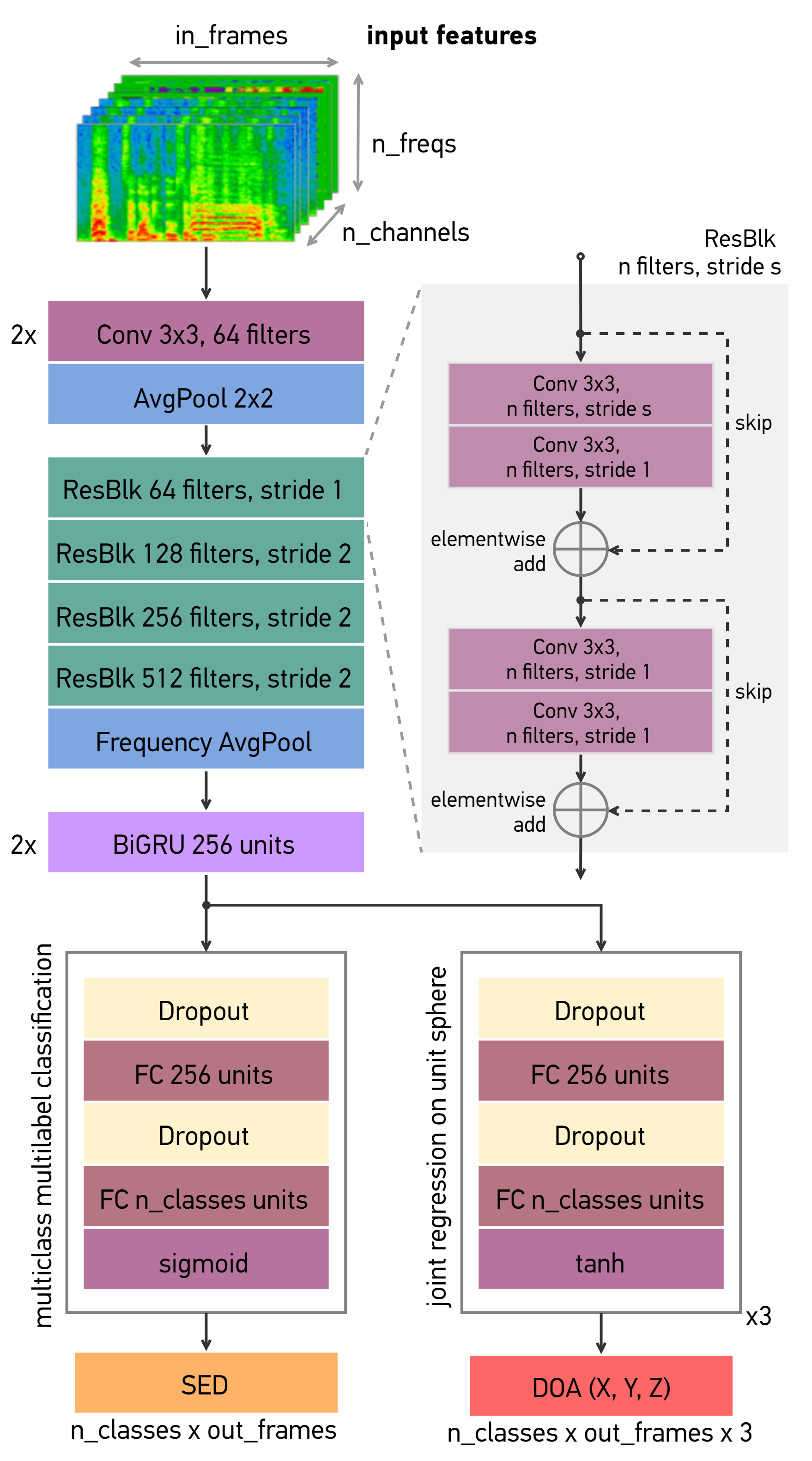
Figure 4: Block diagram of the SELD network, which is a CRNN. This network can be adapted for different input features such as SALSA, MelSpecIV, MelSpecGCC, etc. by changing the number of input channels in the first convolutional layer of the network.

V Experimental Settings

V-A Dataset

The main dataset used in the majority of our experiments is the TNSSE 2021 dataset [Politis2021]. Since this dataset is relatively new, we also use the TNSSE 2020 dataset [Politis2020ADetection] to compare our models with state-of-the-art methods. The development subset of each TNSSE dataset consists of $400$, $100$, and $100$ one-minute audio recordings for the train, validation, and test split, respectively. The evaluation subset of each dataset consists of $200$ one-minute audio recording. Unless otherwise stated, the validation set was used for model selection while the test set was used for evaluation. Table III summarizes some key characteristics of the two datasets. The azimuth and elevation ranges of both datasets are $[$-180\text{\,}\mathrm{\SIUnitSymbolDegree}$,$180\text{\,}\mathrm{\SIUnitSymbolDegree}$)$ and $[$-45\text{\,}\mathrm{\SIUnitSymbolDegree}$,$45\text{\,}\mathrm{\SIUnitSymbolDegree}$]$, respectively.

TABLE III: Characteristics of TNSSE 2020 and 2021 datasets

Characteristics	2020	2021
Channel format	FOA, MIC	FOA, MIC
Moving sources	$\checkmark$	$\checkmark$
Ambiance noise	$\checkmark$	$\checkmark$
Reverberation	$\checkmark$	$\checkmark$
Unknown interferences	$\times$	$\checkmark$
Maximum degree of polyphony	2	3
Number of target sound classes	14	12

Both TNSSE datasets were recorded using a $32$-microphone Eigenmike spherical array with a radius of $4.2\text{\,}\mathrm{cm}$. The $32$-channel signals were converted into FOA format, whose array response is approximately frequency-independent up to around $9\text{\,}\mathrm{kHz}$. Therefore, we compute EIV for SALSA features between $50\text{\,}\mathrm{Hz}$ and $9\text{\,}\mathrm{kHz}$. Out of the $32$ microphones, four microphones that form a tetrahedron are used for the MIC format. Since the radius of the spherical array corresponds to an aliasing frequency of $4\text{\,}\mathrm{kHz}$, we computed EPV for MIC format between $50\text{\,}\mathrm{Hz}$ and $4\text{\,}\mathrm{kHz}$. Even though the microphones are mounted on an acoustically-hard spherical baffle, we found that the far-field array model in Section II-C2 is sufficient to extract the spatial cues for the MIC format.

V-B Evaluation

To evaluate SELD performance, we used the official evaluation metrics [Politis2020Overview2019] that were introduced in the 2021 DCASE Challenge as our default metrics. A sound event is considered a correct detection only if it has correct class prediction and its estimated DOA is less than $D$\mathrm{\SIUnitSymbolDegree}$$ away from the DOA ground truth, where $D=$20\text{\,}\mathrm{\SIUnitSymbolDegree}$$ is the most commonly used value. The DOAE metrics are class-dependent, that is, the detected sound class will have to be correct in order for the corresponding localization predictions to count. Since some state-of-the-art SELD systems only reported the 2020 version of the DCASE evaluation metrics [Mesaros2019JointEvents], we also used these metrics in some experiments to fairly compare the results.

Both the 2020 and 2021 SELD evaluation metrics consist of four metrics: location-dependent error rate ($\text{ER}_{\leq$20\text{\,}\mathrm{\SIUnitSymbolDegree}$}$) and F1 score ($\text{F}_{\leq$20\text{\,}\mathrm{\SIUnitSymbolDegree}$}$) for SED; and class-dependent localization error ($\text{LE}_{\text{CD}}$), and localization recall ($\text{LR}_{\text{CD}}$) for DOAE. We also computed an aggregated SELD error metric that was used as the ranking metric for the 2019 and 2020 DCASE Challenges as follows,

$$\mathcal{E}_{\textsc{seld}}=\dfrac{1}{4}\left[\text{ER}_{\leq$20\text{\,}\mathrm{\SIUnitSymbolDegree}$}+(1-\text{F}_{\leq$20\text{\,}\mathrm{\SIUnitSymbolDegree}$})+\dfrac{\text{LE}_{\textsc{cd}}}{$180\text{\,}\mathrm{\SIUnitSymbolDegree}$}+(1-\text{LR}_{\textsc{cd}})\right].$$ (16)

$\mathcal{E}_{\text{SELD}}$ was used for model and hyperparameter selection. A good SELD system should have low $\text{ER}_{\leq$20\text{\,}\mathrm{\SIUnitSymbolDegree}$}$, high $\text{F}_{\leq$20\text{\,}\mathrm{\SIUnitSymbolDegree}$}$, low $\text{LE}_{\text{CD}}$, high $\text{LR}_{\text{CD}}$, and low aggregated error metric $\mathcal{E}_{\text{SELD}}$.

V-C Hyperparameters

We used a sampling rate of $24\text{\,}\mathrm{kHz}$, window length of $512\text{\,}\mathrm{s}\mathrm{a}\mathrm{m}\mathrm{p}\mathrm{l}\mathrm{e}\mathrm{s}$, hop length of $300\text{\,}\mathrm{s}\mathrm{a}\mathrm{m}\mathrm{p}\mathrm{l}\mathrm{e}\mathrm{s}$, Hann window, $512$ FFT points, and $128$ mel bands. As a result, the input frame rate of all the features was $80\text{\,}\mathrm{f}\mathrm{p}\mathrm{s}$. Since the model temporally downsampled the input by a factor of $16$, we temporally upsampled the final outputs by a factor of $2$ to match the label frame rate of $10\text{\,}\mathrm{f}\mathrm{p}\mathrm{s}$. To reduce the feature dimensions to speed up the training time, we linearly compressed frequency bands above $9\text{\,}\mathrm{kHz}$, which correspond to frequency bin index $192$ and above, by a factor of $8$, i.e., $8$ consecutive bands will be averaged into a single band. As the results, the frequency dimension is $F=200$ for all linear-scale features. Unless stated otherwise, $8$-second audio chunks were used for model training. The loss weights for SED and DOAE were set to $\lambda=0.3$ and $\gamma=0.7$, respectively. Adam optimizer was used for all training. The learning rate was initially set to $3\text{\times}{10}^{-4}$ and linearly decreased to ${10}^{-4}$ over last $15$ epochs of the total $50$ training epochs. A threshold of $0.3$ was used to binarize active class predictions in the SED outputs.

VI Results and discussion

We performed a series of experiments to compare the performances of each input feature with and without data augmentation. Afterwards, the effect of data augmentation on each feature was examined in details. We analyzed the effects of the magnitude and coherence tests on the performance of SELD systems running on SALSA features. Next, we studied the feature importance of LinSpec, EIV and EPV that constitute SALSA features. In addition, effect of different segment lengths on SALSA performance was investigated. For the MIC format, we examined effect of spatial aliasing on the SELD performance with SALSA features. Finally, we compared the performance of models trained on the proposed SALSA features with several state-of-the-art SELD systems on both the 2020 and 2021 TNSSE datasets.

VI-A Comparison between SALSA and other SELD features

TABLE IV: Baseline SELD performances of different features without data augmentation.

Feature	Data Aug.	FOA format					MIC format
		$\downarrow$ $\text{ER}_{\leq$20\text{\,}\mathrm{\SIUnitSymbolDegree}$}$	$\uparrow$ $\text{F}_{\leq$20\text{\,}\mathrm{\SIUnitSymbolDegree}$}$	$\downarrow$ $\text{LE}_{\text{CD}}$	$\uparrow$ $\text{LR}_{\text{CD}}$	$\downarrow$ $\mathcal{E}_{\text{SELD}}$	$\downarrow$ $\text{ER}_{\leq$20\text{\,}\mathrm{\SIUnitSymbolDegree}$}$	$\uparrow$ $\text{F}_{\leq$20\text{\,}\mathrm{\SIUnitSymbolDegree}$}$	$\downarrow$ $\text{LE}_{\text{CD}}$	$\uparrow$ $\text{LR}_{\text{CD}}$	$\downarrow$ $\mathcal{E}_{\text{SELD}}$
MelSpecIV	None	0.555	0.584	15.9$\mathrm{\SIUnitSymbolDegree}$	0.625	0.358	-	-	-	-	-
LinSpecIV	None	0.527	0.609	15.6$\mathrm{\SIUnitSymbolDegree}$	0.642	0.341	-	-	-	-	-
MelSpecGCC	None	-	-	-	-	-	0.660	0.455	21.1$\mathrm{\SIUnitSymbolDegree}$	0.521	0.450
LinSpecGCC	None	-	-	-	-	-	0.622	0.506	19.6$\mathrm{\SIUnitSymbolDegree}$	0.583	0.410
FOA SALSA	None	0.543	0.592	15.4$\mathrm{\SIUnitSymbolDegree}$	0.627	0.352	-	-	-	-	-
MIC SALSA	None	-	-	-	-	-	0.528	0.601	15.9$\mathrm{\SIUnitSymbolDegree}$	0.644	0.343

TABLE V: SELD performances of different features with best combination of data augmentation techniques.

Feature	Data Aug.	FOA format					MIC format
		$\downarrow$ $\text{ER}_{\leq$20\text{\,}\mathrm{\SIUnitSymbolDegree}$}$	$\uparrow$ $\text{F}_{\leq$20\text{\,}\mathrm{\SIUnitSymbolDegree}$}$	$\downarrow$ $\text{LE}_{\text{CD}}$	$\uparrow$ $\text{LR}_{\text{CD}}$	$\downarrow$ $\mathcal{E}_{\text{SELD}}$	$\downarrow$ $\text{ER}_{\leq$20\text{\,}\mathrm{\SIUnitSymbolDegree}$}$	$\uparrow$ $\text{F}_{\leq$20\text{\,}\mathrm{\SIUnitSymbolDegree}$}$	$\downarrow$ $\text{LE}_{\text{CD}}$	$\uparrow$ $\text{LR}_{\text{CD}}$	$\downarrow$ $\mathcal{E}_{\text{SELD}}$
MelSpecIV	CS + FS	0.444	0.686	11.8$\mathrm{\SIUnitSymbolDegree}$	0.686	0.284	-	-	-	-	-
LinSpecIV	CS + FS + RC	0.410	0.710	10.5$\mathrm{\SIUnitSymbolDegree}$	0.702	0.264	-	-	-	-	-
MelSpecGCC	CS + FS + RC	-	-	-	-	-	0.507	0.614	17.9$\mathrm{\SIUnitSymbolDegree}$	0.679	0.328
LinSpecGCC	CS + FS + RC	-	-	-	-	-	0.514	0.606	17.8$\mathrm{\SIUnitSymbolDegree}$	0.676	0.333
FOA SALSA	CS + FS	0.404	0.724	12.5$\mathrm{\SIUnitSymbolDegree}$	0.727	0.255	-	-	-	-	-
MIC SALSA	CS + FS + RC	-	-	-	-	-	0.408	0.715	12.6$\mathrm{\SIUnitSymbolDegree}$	0.728	0.259
CS: channel swapping; FS: frequency shifting; RC: random cutout.

Table IV shows benchmark performances of all considered features without data augmentation. Linear-scale features (LinSpec-based) appear to perform better than their mel-scale counterparts (MelSpec-based) for both audio formats. For the ‘traditional’ features, the performance gap between the FOA and MIC formats is large, with both IV-based features outperforming GCC-based features. Without data augmentation, FOA SALSA performed better than MelSpecIV but slightly worse than LinSpecIV, while MIC SALSA performed much better than both GCC-based features.

Table V shows the performance of all features with their respective best combination of the three data augmentation techniques investigated. For the FOA format, the experimental results, again, showed that linear-scale features achieved better performance than mel-scale features. For the MIC format, the mel-scale features performed slightly better than linear-scale features. The large performance gap between the FOA and MIC formats still remained with data augmentation applied. IV-based features significantly outperform GCC-based features across all the evaluation metrics. With data augmentation, the proposed SALSA features achieved the best overall performances for both the FOA and MIC formats. SALSA scored the highest in $\text{F}_{\leq$20\text{\,}\mathrm{\SIUnitSymbolDegree}$}$ and $\text{LR}_{\text{CD}}$; and the lowest in $\text{ER}_{\leq$20\text{\,}\mathrm{\SIUnitSymbolDegree}$}$ and $\mathcal{E}_{\text{SELD}}$ among the setups investigated in Table V. It is expected that a high $\text{LR}_{\text{CD}}$ often leads to a high $\text{LE}_{\text{CD}}$. With a higher $\text{LR}_{\text{CD}}$, SALSA also has a higher $\text{LE}_{\text{CD}}$ than LinSpecIV by $2\text{\,}\mathrm{\SIUnitSymbolDegree}$. SALSA outperformed both GCC-based features by a large margin. Compared to MelSpecGCC, SALSA feature substantially reduced $\text{ER}_{\leq$20\text{\,}\mathrm{\SIUnitSymbolDegree}$}$ by $20\text{\,}\mathrm{\char 37\relax}$, increased $\text{F}_{\leq$20\text{\,}\mathrm{\SIUnitSymbolDegree}$}$ by $16\text{\,}\mathrm{\char 37\relax}$, reduced $\text{LE}_{\text{CD}}$ by $5.3\text{\,}\mathrm{\SIUnitSymbolDegree}$, and increased $\text{LR}_{\text{CD}}$ by $7\text{\,}\mathrm{\char 37\relax}$. The overall $\mathcal{E}_{\text{SELD}}$ was impressively reduced by $21\text{\,}\mathrm{\char 37\relax}$.

The performance gap between the IV- and GCC-based features, and the similar performances of SALSA for both array formats indicated that the exact TF mapping between the signal power and the directional cues, as per SALSA, MelSpecIV, and LinSpecIV, are much better for SELD than simply stacking spectrograms and GCC-PHAT spectra as per MelSpecGCC and LinSpecGCC. This exact TF mapping also facilitates the learning of CNNs, as the filters can more conveniently learn the multichannel local patterns on the image-like input features. Most importantly, the results showed that the extracted spatial cues for SALSA features are effective for both FOA and MIC formats. Therefore, SALSA can be considered as a unified SELD feature regardless of the array format. The outstanding performance gains in models trained with SALSA features shown in both Table IV and V indicate that SALSA as a very effective feature for deep learning-based SELD.

VI-B Effect of data augmentation

We report the effect of different data augmentation techniques on each feature in Table VI. The experimental results clearly demonstrated that channel swapping significantly improved the performance for all features across all metrics. On average, $\text{ER}_{\leq$20\text{\,}\mathrm{\SIUnitSymbolDegree}$}$ decreased by $14.8\text{\,}\mathrm{\char 37\relax}$, $\text{F}_{\leq$20\text{\,}\mathrm{\SIUnitSymbolDegree}$}$ increased by $13.8\text{\,}\mathrm{\char 37\relax}$, $\text{LE}_{\text{CD}}$ decreased by $2.3\text{\,}\mathrm{\SIUnitSymbolDegree}$, and $\text{LR}_{\text{CD}}$ increased by $7.8\text{\,}\mathrm{\char 37\relax}$. Channel swapping reduced the aggregated error metric $\mathcal{E}_{\text{SELD}}$ by between $13\text{\,}\mathrm{\char 37\relax}$ and $16\text{\,}\mathrm{\char 37\relax}$, where the larger reductions are observed for MIC features such as MelSpecGCC, LinSpecGCC, and MIC SALSA.

When frequency shifting was used together with channel swapping, the performance was improved further for all features. Compared to channel swapping alone, the combination of channel swapping and frequency shifting on average reduced $\text{ER}_{\leq$20\text{\,}\mathrm{\SIUnitSymbolDegree}$}$ by a further $7.3\text{\,}\mathrm{\char 37\relax}$, increased $\text{F}_{\leq$20\text{\,}\mathrm{\SIUnitSymbolDegree}$}$ by $5.8\text{\,}\mathrm{\char 37\relax}$, reduced $\text{LE}_{\text{CD}}$ by $1.2\text{\,}\mathrm{\SIUnitSymbolDegree}$, increased $\text{LR}_{\text{CD}}$ by $5.3\text{\,}\mathrm{\char 37\relax}$, and reduced $\mathcal{E}_{\text{SELD}}$ by $8.6\text{\,}\mathrm{\char 37\relax}$. These results showed that varying the SED and DOA patterns by frequency shifting and channel swapping helped the models learn more effectively.

When random cutout was used together with channel swapping and frequency shifting, the performance was further improved for LinSpecIV and all MIC features; but not for MelSpecIV and FOA SALSA. For subsequent experiments, the best combinations of data augmentation techniques for each feature, as shown in boldface in Table VI, are used.

TABLE VI: Performance of MelSpecIV, LinSpecIV, MelSpecGCC, LinSpecGCC, and SALSA with different data augmentation.

Data Aug.	$\downarrow\text{ER}_{\leq$20\text{\,}\mathrm{\SIUnitSymbolDegree}$}$	$\uparrow\text{F}_{\leq$20\text{\,}\mathrm{\SIUnitSymbolDegree}$}$	$\downarrow\text{LE}_{\text{CD}}$	$\uparrow\text{LR}_{\text{CD}}$	$\downarrow\mathcal{E}_{\text{SELD}}$
MelSpecIV
None	0.555	0.584	15.9$\mathrm{\SIUnitSymbolDegree}$	0.625	0.358
CS	0.472	0.655	12.0$\mathrm{\SIUnitSymbolDegree}$	0.653	0.308
CS+FS	0.444	0.686	11.8$\mathrm{\SIUnitSymbolDegree}$	0.686	0.284
CS+FS+RC	0.440	0.683	10.2$\mathrm{\SIUnitSymbolDegree}$	0.668	0.286
LinSpecIV
None	0.527	0.609	15.6$\mathrm{\SIUnitSymbolDegree}$	0.642	0.341
CS	0.459	0.669	12.3$\mathrm{\SIUnitSymbolDegree}$	0.678	0.295
CS+FS	0.423	0.700	10.8$\mathrm{\SIUnitSymbolDegree}$	0.692	0.273
CS+FS+RC	0.410	0.710	10.5$\mathrm{\SIUnitSymbolDegree}$	0.702	0.264
FOA SALSA
None	0.543	0.592	15.4$\mathrm{\SIUnitSymbolDegree}$	0.627	0.352
SC	0.462	0.655	14.9$\mathrm{\SIUnitSymbolDegree}$	0.666	0.306
CS+FS	0.404	0.724	12.5$\mathrm{\SIUnitSymbolDegree}$	0.727	0.255
CS+FS+RC	0.413	0.713	11.5$\mathrm{\SIUnitSymbolDegree}$	0.713	0.263
MelSpecGCC
None	0.660	0.455	21.1$\mathrm{\SIUnitSymbolDegree}$	0.521	0.450
CS	0.552	0.556	18.1$\mathrm{\SIUnitSymbolDegree}$	0.583	0.378
CS+FS	0.507	0.609	17.0$\mathrm{\SIUnitSymbolDegree}$	0.646	0.337
CS+FS+RC	0.507	0.614	17.9$\mathrm{\SIUnitSymbolDegree}$	0.679	0.328
LinSpecGCC
None	0.622	0.506	19.6$\mathrm{\SIUnitSymbolDegree}$	0.583	0.410
CS	0.532	0.589	18.6$\mathrm{\SIUnitSymbolDegree}$	0.658	0.347
CS+FS	0.514	0.604	17.7$\mathrm{\SIUnitSymbolDegree}$	0.666	0.336
CS+FS+RC	0.514	0.606	17.8$\mathrm{\SIUnitSymbolDegree}$	0.676	0.333
MIC SALSA
None	0.528	0.601	15.9$\mathrm{\SIUnitSymbolDegree}$	0.644	0.343
CS	0.447	0.675	13.7$\mathrm{\SIUnitSymbolDegree}$	0.683	0.291
CS+FS	0.431	0.696	12.3$\mathrm{\SIUnitSymbolDegree}$	0.709	0.274
CS+FS+RC	0.408	0.715	12.6$\mathrm{\SIUnitSymbolDegree}$	0.728	0.259
CS: channel swapping; FS: frequency shifting; RC: random cutout.

VI-C Effect of magnitude and coherence tests

TABLE VII: Effect of magnitude and coherence tests on SALSA features.

Test	$\downarrow$ $\text{ER}_{\leq$20\text{\,}\mathrm{\SIUnitSymbolDegree}$}$	$\uparrow$ $\text{F}_{\leq$20\text{\,}\mathrm{\SIUnitSymbolDegree}$}$	$\downarrow$ $\text{LE}_{\text{CD}}$	$\uparrow$ $\text{LR}_{\text{CD}}$	$\downarrow$ $\mathcal{E}_{\text{SELD}}$
FOA SALSA
None	0.418	0.706	12.0$\mathrm{\SIUnitSymbolDegree}$	0.710	0.267
Magnitude	0.434	0.698	11.9$\mathrm{\SIUnitSymbolDegree}$	0.701	0.275
Magnitude + Coherence	0.404	0.724	12.5$\mathrm{\SIUnitSymbolDegree}$	0.727	0.255
MIC SALSA
None	0.414	0.701	12.1$\mathrm{\SIUnitSymbolDegree}$	0.700	0.270
Magnitude	0.407	0.716	12.3$\mathrm{\SIUnitSymbolDegree}$	0.721	0.260
Magnitude + Coherence	0.408	0.715	12.6$\mathrm{\SIUnitSymbolDegree}$	0.728	0.259
CS: channel swapping; FS: frequency shifting; RC: random cutout.

Table VII shows the effect of magnitude and coherence tests on the performance of models trained on SALSA features. Fig. 3 indicates that around $33\text{\,}\mathrm{\char 37\relax}$ of all TF bins are removed after the magnitude test, and an additional $20\text{\,}\mathrm{\char 37\relax}$ of bins are removed after the coherence test. These tests aim to only include approximately single-source TF bins with reliable directional cues. The magnitude test improved the performance of the MIC format but not the FOA format. On the other hand, using both the magnitude and coherence tests significantly improved the performance of the FOA format. Overall, when both tests are applied to compute SALSA features, the performances were improved compared to when no test was applied. For subsequent experiments, both tests were applied to compute SALSA features.

VI-D Feature importance

TABLE VIII: Feature importance of FOA and MIC SALSA.

Components	$\downarrow\text{ER}_{\leq$20\text{\,}\mathrm{\SIUnitSymbolDegree}$}$	$\uparrow\text{F}_{\leq$20\text{\,}\mathrm{\SIUnitSymbolDegree}$}$	$\downarrow\text{LE}_{\text{CD}}$	$\uparrow\text{LR}_{\text{CD}}$	$\downarrow\mathcal{E}_{\text{SELD}}$
FOA SALSA
LinSpec	0.835	0.123	87.2$\mathrm{\SIUnitSymbolDegree}$	0.608	0.647
EIV	0.577	0.557	14.1$\mathrm{\SIUnitSymbolDegree}$	0.571	0.382
Mono-SALSA	0.421	0.705	12.8$\mathrm{\SIUnitSymbolDegree}$	0.723	0.266
SALSA	0.404	0.724	12.5$\mathrm{\SIUnitSymbolDegree}$	0.727	0.255
MIC SALSA
LinSpec	0.506	0.616	18.1$\mathrm{\SIUnitSymbolDegree}$	0.698	0.323
EPV	0.629	0.502	17.4$\mathrm{\SIUnitSymbolDegree}$	0.547	0.419
Mono-SALSA	0.443	0.680	14.7$\mathrm{\SIUnitSymbolDegree}$	0.710	0.284
SALSA	0.408	0.715	12.6$\mathrm{\SIUnitSymbolDegree}$	0.728	0.259

Table VIII reports the feature importance of each component in SALSA feature: multichannel log-linear spectrogram LinSpec, as well as spatial features EIV and EPV for FOA and MIC formats, respectively. Mono-SALSA is an ablation feature formed by stacking the log-linear spectrogram of only the first microphone with the corresponding spatial features. For both formats, SALSA achieved the best performance, followed by Mono-SALSA.

For the FOA format, LinSpec alone could not meaningfully estimate DOAs. One possible reason is that the spatial cues of FOA format are encoded in the signed amplitude differences between microphones, but LinSpec retains only the unsigned magnitude differences. The sign ambiguity caused the confusion between the input features and the target labels. Therefore, the model trained on LinSpec feature failed to detect the correct DOAs. On the other hand, the model trained on only the EIV feature performed reasonably well. The EIV feature preserved some coarse spatiotemporal patterns of each sound class (see Fig. 1), thus the model was able to distinguish different sound classes. SALSA feature significantly outperformed its constituent features, LinSpec and EIV. In the absence of the X, Y, and Z channels of the linear spectrograms, Mono-SALSA performed slightly worse than SALSA on the SED metrics but similarly on the DOAE metrics. These results suggest that the main contribution of the X, Y, and Z channels in the linear spectrograms is to distinguish different sound classes.

For the MIC format, LinSpec alone performed reasonably well for SELD. Referring to Section V-A, the MIC format of the DCASE SELD dataset is not a true far-field array, but rather a baffled microphone array, where some spatial cues are also encoded in the magnitude differences between microphones. Therefore, not only is the model trained on LinSpec feature able to classify sound sources, but it is also able to estimate DOAs. The EPV feature alone returned a lower SELD performance compared to the EIV feature of the FOA format, likely because the EPV feature is computed with an upper cutoff frequency of $4\text{\,}\mathrm{kHz}$, which is much lower than that of EIV at $9\text{\,}\mathrm{kHz}$. The model trained on only EPV also has the highest $\text{ER}_{\leq$20\text{\,}\mathrm{\SIUnitSymbolDegree}$}$ and lowest $\text{F}_{\leq$20\text{\,}\mathrm{\SIUnitSymbolDegree}$}$ among all ablation models of the MIC format. SALSA feature significantly outperformed its individual feature component across all the metrics. The performance gap between SALSA and Mono-SALSA is larger for the MIC format than the FOA format. The reason is likely that the spatial cues are also encoded in the magnitude of different input channels, and the EPV is all zeroed out above the upper cutoff frequency. Therefore, the multichannel nature of the spectrograms play an important role in both sound class recognition and DOA estimation.

VI-E Effect of spatial aliasing on SELD for microphone array

TABLE IX: Effect of spatial aliasing on SALSA feature of MIC format.

Cutoff frequency	$\downarrow\text{ER}_{\leq$20\text{\,}\mathrm{\SIUnitSymbolDegree}$}$	$\uparrow\text{F}_{\leq$20\text{\,}\mathrm{\SIUnitSymbolDegree}$}$	$\downarrow\text{LE}_{\text{CD}}$	$\uparrow\text{LR}_{\text{CD}}$	$\downarrow\mathcal{E}_{\text{SELD}}$
$2.0\text{\,}\mathrm{kHz}$	0.403	0.714	12.5$\mathrm{\SIUnitSymbolDegree}$	0.707	0.261
$4.0\text{\,}\mathrm{kHz}$	0.408	0.715	12.6$\mathrm{\SIUnitSymbolDegree}$	0.728	0.259
$9.0\text{\,}\mathrm{kHz}$	0.425	0.698	12.8$\mathrm{\SIUnitSymbolDegree}$	0.720	0.270

For narrow band signals, spatial aliasing occurs at high frequency bins, where half of the signal wavelength is less than the distance between two microphones. To investigate the effect of spatial aliasing when SALSA features for MIC format are used, we report the performances of SALSA with different upper cutoff frequencies in Table IX. The upper cutoff frequencies were computed using the spatial aliasing formula for narrow band signals, $f_{\text{alias}}=c/(2d_{\text{max}})$, where $d_{\text{max}}$ is the maximum distance between any two microphones in the array. The investigated values of $d_{\text{max}}$ are the arc length between any two microphones ($8.0\text{\,}\mathrm{cm}$) and the radius of the Eigenmike array ($4.2\text{\,}\mathrm{cm}$), which correspond to aliasing frequencies of $2\text{\,}\mathrm{kHz}$, and $4\text{\,}\mathrm{kHz}$, respectively. In addition, we also tested a cutoff frequency of $9\text{\,}\mathrm{kHz}$ to investigate the case where spatial aliasing is ignored. Table IX shows that cutoff frequencies at $2\text{\,}\mathrm{kHz}$ and $4\text{\,}\mathrm{kHz}$ result in similar performances. One possible reason is that the spatial aliasing might not significantly occur in all of the microphone pairs beyond $2\text{\,}\mathrm{kHz}$ for some DOAs. On the other hand, with the $9\text{\,}\mathrm{kHz}$ cutoff frequency, spatial aliasing has occurred in too many high-frequency bins, resulting in a slightly lower performance than a loose cutoff frequency at $4\text{\,}\mathrm{kHz}$. However, the impact of spatial aliasing appears to be mild, with the model trained on a loose aliasing frequency at $4\text{\,}\mathrm{kHz}$ achieving the best $\mathcal{E}_{\text{SELD}}$. This result is agreeable with the finding in [Dmochowski2009OnArrays], where broadband signals were shown to not experience spatial aliasing unless they contain strong harmonic components.

VI-F Effect of segment length for training

TABLE X: Effect of segment length during training on SELD performance using SALSA.

Length	$\downarrow$ $\text{ER}_{\leq$20\text{\,}\mathrm{\SIUnitSymbolDegree}$}$	$\uparrow$ $\text{F}_{\leq$20\text{\,}\mathrm{\SIUnitSymbolDegree}$}$	$\downarrow$ $\text{LE}_{\text{CD}}$	$\uparrow$ $\text{LR}_{\text{CD}}$	$\downarrow$ $\mathcal{E}_{\text{SELD}}$
FOA SALSA
$4\text{\,}\mathrm{s}$	0.468	0.658	13.4$\mathrm{\SIUnitSymbolDegree}$	0.646	0.310
$8\text{\,}\mathrm{s}$	0.404	0.724	12.5$\mathrm{\SIUnitSymbolDegree}$	0.727	0.255
$12\text{\,}\mathrm{s}$	0.414	0.717	11.8$\mathrm{\SIUnitSymbolDegree}$	0.720	0.261
MIC SALSA
$4\text{\,}\mathrm{s}$	0.449	0.664	14.1$\mathrm{\SIUnitSymbolDegree}$	0.678	0.297
$8\text{\,}\mathrm{s}$	0.408	0.715	12.6$\mathrm{\SIUnitSymbolDegree}$	0.728	0.259
$12\text{\,}\mathrm{s}$	0.413	0.714	12.7$\mathrm{\SIUnitSymbolDegree}$	0.730	0.260

Different sound events often have different duration. Thus the segment length that is used during training may affect the model performance. The sound event lengths from the TNSSE 2021 dataset are between $0.2\text{\,}\mathrm{s}$ and $40.0\text{\,}\mathrm{s}$, with a median of $3.2\text{\,}\mathrm{s}$, and a mean of $8.3\text{\,}\mathrm{s}$. We present the SELD performances on models trained with different input segment lengths, as per Table X. Models trained with a segment length of $8\text{\,}\mathrm{s}$ significantly outperformed models trained with a segment length of $4\text{\,}\mathrm{s}$ for both the FOA and MIC formats. However, increasing the segment length to $12\text{\,}\mathrm{s}$ did not further improve the overall performance. Thus, it appears that the model requires a certain minimum sequence length to sufficiently learn the temporal dependency, although this temporal dependency does not need to be very long, since the model would likely rely more on recent frames than older frames.

VI-G Comparisons with state-of-the-art methods for SELD

We compared models trained with the proposed SALSA features with state-of-the-art (SOTA) methods on three datasets: the test and evaluation splits of the TNSSE 2020 dataset [Politis2020ADetection] and the test split of the TNSSE 2021 dataset [Politis2021]. Some of the SOTA methods used single models while others used ensemble models. We used the same single-model SELD network shown in Section IV to train all of the models reported, i.e., no ensembling was used. To further improve the performance of our models, we applied test-time augmentation (TTA) during inference [Shimada2021ACCDOA:Detection]. TTA swaps the channels of the SALSA features in a manner similar to the channel swapping augmentation technique that was employed during training. The estimated DOA outputs were rotated back to the original axes, then averaged to produce the final results. During inference, the whole $60$-second features were passed into the models without being split into smaller chunks. Since the SOTA results on the TNSSE 2020 dataset were evaluated using the 2020 SELD evaluation metrics, we evaluated our models using both the 2020 and 2021 metrics, the former for fair comparison with past works, and the latter for ease of comparison with future works.

VI-G1 Performance on the test split of the TNSSE 2020 dataset

TABLE XI: SELD performances of SOTA systems and SALSA-based models on test split of the TNSSE 2020 dataset.

System	Format	$\text{ER}_{\leq$20\text{\,}\mathrm{\SIUnitSymbolDegree}$}$	$\text{F}_{\leq$20\text{\,}\mathrm{\SIUnitSymbolDegree}$}$	$\text{LE}_{\text{CD}}$	$\text{LR}_{\text{CD}}$
2020 Metrics
DCASE baseline [Politis2020ADetection]	FOA	0.72	0.374	22.8$\mathrm{\SIUnitSymbolDegree}$	0.607
Shimada et al. [Shimada2021ACCDOA:Detection] w/o TTA	FOA	0.36	0.730	10.2$\mathrm{\SIUnitSymbolDegree}$	0.791
Shimada et al. [Shimada2021ACCDOA:Detection] w/ TTA	FOA	0.32	0.768	7.9$\mathrm{\SIUnitSymbolDegree}$	0.805
Wang et al. [Wang2020TheChallenge]	FOA+MIC	0.29	0.764	9.4$\mathrm{\SIUnitSymbolDegree}$	0.828
(’20 #1) Wang et al. [Wang2020TheChallenge] $\star$	FOA+MIC	0.26	0.800	7.4$\mathrm{\SIUnitSymbolDegree}$	0.847
FOA SALSA w/o TTA	FOA	0.338	0.748	7.9$\mathrm{\SIUnitSymbolDegree}$	0.784
MIC SALSA w/o TTA	MIC	0.379	0.717	8.2$\mathrm{\SIUnitSymbolDegree}$	0.762
FOA SALSA w/ TTA	FOA	0.318	0.761	7.4$\mathrm{\SIUnitSymbolDegree}$	0.797
MIC SALSA w/ TTA	MIC	0.341	0.741	7.8$\mathrm{\SIUnitSymbolDegree}$	0.783
2021 Metrics
FOA SALSA w/o TTA	FOA	0.344	0.755	8.1$\mathrm{\SIUnitSymbolDegree}$	0.755
MIC SALSA w/o TTA	MIC	0.383	0.727	8.3$\mathrm{\SIUnitSymbolDegree}$	0.738
FOA SALSA w/ TTA	FOA	0.323	0.768	7.5$\mathrm{\SIUnitSymbolDegree}$	0.763
MIC SALSA w/ TTA	MIC	0.342	0.749	7.9$\mathrm{\SIUnitSymbolDegree}$	0.744
$\star$ denotes an ensemble model.

Table XI shows the performances on the test split of the TNSSE 2020 dataset of SOTA systems, and our SALSA models for both the FOA and MIC formats. FOA SALSA models performed slightly better than the MIC counterparts. The TTA significantly improved location dependent SED metrics $\text{ER}_{\leq$20\text{\,}\mathrm{\SIUnitSymbolDegree}$}$ and $\text{F}_{\leq$20\text{\,}\mathrm{\SIUnitSymbolDegree}$}$. The model by Wang et al. [Wang2020TheChallenge] used both the FOA and MIC data as input features and achieved the best performance for $\text{ER}_{\leq$20\text{\,}\mathrm{\SIUnitSymbolDegree}$}$, $\text{F}_{\leq$20\text{\,}\mathrm{\SIUnitSymbolDegree}$}$, and $\text{LR}_{\text{CD}}$ for single models. However, it is considerably more expensive to have both FOA and MIC data available in real-life applications due to the more specialized recording setup required. Our FOA SALSA model outperformed the DCASE baseline [Politis2020ADetection] by a large margin, and performed better than [Shimada2021ACCDOA:Detection] in term of $\text{ER}_{\leq$20\text{\,}\mathrm{\SIUnitSymbolDegree}$}$, $\text{F}_{\leq$20\text{\,}\mathrm{\SIUnitSymbolDegree}$}$, and $\text{LE}_{\text{CD}}$. Our FOA SALSA model with TTA also performed on-par with the TTA version of [Shimada2021ACCDOA:Detection]. On average, the 2021 evaluation metrics return similar $\text{ER}_{\leq$20\text{\,}\mathrm{\SIUnitSymbolDegree}$}$, $\text{F}_{\leq$20\text{\,}\mathrm{\SIUnitSymbolDegree}$}$ and $\text{LE}_{\text{CD}}$ compared to the 2020 metrics, but stricter $\text{LR}_{\text{CD}}$ than the 2020 metrics.

VI-G2 Performance on the evaluation split of the TNSSE 2020 dataset

TABLE XII: SELD performances of SOTA systems and SALSA-based models on evaluation split of TNSSE 2020 dataset.

System	Format	$\text{ER}_{\leq$20\text{\,}\mathrm{\SIUnitSymbolDegree}$}$	$\text{F}_{\leq$20\text{\,}\mathrm{\SIUnitSymbolDegree}$}$	$\text{LE}_{\text{CD}}$	$\text{LR}_{\text{CD}}$
2020 Metrics
DCASE’21 baseline [Politis2020ADetection]	MIC	0.69	0.413	23.1$\mathrm{\SIUnitSymbolDegree}$	0.624
Cao et al. [12]	FOA	0.233	0.832	6.8$\mathrm{\SIUnitSymbolDegree}$	0.861
(’20 #2) Nguyen et al. [Nguyen2020EnsembleTracking] $\star$	FOA	0.23	0.820	9.3$\mathrm{\SIUnitSymbolDegree}$	0.900
(’20 #1) Wang et al. [Wang2020TheChallenge] $\star$	FOA+MIC	0.20	0.849	6.0$\mathrm{\SIUnitSymbolDegree}$	0.885
FOA SALSA w/o TTA	FOA	0.237	0.823	6.9$\mathrm{\SIUnitSymbolDegree}$	0.858
MIC SALSA w/o TTA	MIC	0.227	0.836	6.7$\mathrm{\SIUnitSymbolDegree}$	0.869
FOA SALSA w/ TTA	FOA	0.219	0.840	6.5$\mathrm{\SIUnitSymbolDegree}$	0.869
MIC SALSA w/ TTA	MIC	0.202	0.854	6.0$\mathrm{\SIUnitSymbolDegree}$	0.884
2021 Metrics
FOA SALSA w/o TTA	FOA	0.244	0.830	7.0$\mathrm{\SIUnitSymbolDegree}$	0.831
MIC SALSA w/o TTA	MIC	0.234	0.842	6.7$\mathrm{\SIUnitSymbolDegree}$	0.849
FOA SALSA w/ TTA	FOA	0.225	0.844	6.6$\mathrm{\SIUnitSymbolDegree}$	0.838
MIC SALSA w/ TTA	MIC	0.208	0.858	6.0$\mathrm{\SIUnitSymbolDegree}$	0.856
$\star$ denotes an ensemble model.

Table XII shows the performances on the evaluation split of the TNSSE 2020 dataset of SOTA systems, and our SALSA models for both the FOA and MIC formats. Our models were trained using all $600$ audio clips from the development split of the TNSSE 2020 dataset. Interestingly, when more data are available for training, models trained on MIC SALSA features performed better than models trained on FOA SALSA features across all metrics. The FOA SALSA model has competitive performance compared to [12] while the MIC SALSA model performed slightly better. The MIC SALSA model with TTA achieved comparable performance as the top ensemble model [Wang2020TheChallenge] from the 2020 DCASE Challenge, with similar $\text{ER}_{\leq$20\text{\,}\mathrm{\SIUnitSymbolDegree}$}$, $\text{LE}_{\text{CD}}$, $\text{LR}_{\text{CD}}$ and higher $\text{F}_{\leq$20\text{\,}\mathrm{\SIUnitSymbolDegree}$}$. The 2021 metrics again returned similar $\text{ER}_{\leq$20\text{\,}\mathrm{\SIUnitSymbolDegree}$}$, $\text{F}_{\leq$20\text{\,}\mathrm{\SIUnitSymbolDegree}$}$, $\text{LE}_{\text{CD}}$ results and stricter $\text{LR}_{\text{CD}}$ than the 2020 metrics.

VI-G3 Performance on the test split of the TNSSE 2021 dataset

TABLE XIII: SELD performances of SOTA systems and SALSA-based models on test split of TNSSE 2021 dataset.

System	Format	$\text{ER}_{\leq$20\text{\,}\mathrm{\SIUnitSymbolDegree}$}$	$\text{F}_{\leq$20\text{\,}\mathrm{\SIUnitSymbolDegree}$}$	$\text{LE}_{\text{CD}}$	$\text{LR}_{\text{CD}}$
2021 Metrics
DCASE baseline [Politis2021]	FOA	0.73	0.307	24.5$\mathrm{\SIUnitSymbolDegree}$	0.448
(’21 #1) Shimada et al. [Shimada2021EnsembleDetection] $\star$	FOA	0.43	0.699	11.1$\mathrm{\SIUnitSymbolDegree}$	0.732
(’21 #4) Lee et al. [Lee2021SoundChallenge] $\star$	FOA	0.46	0.609	14.4$\mathrm{\SIUnitSymbolDegree}$	0.733
FOA SALSA w/o TTA	FOA	0.404	0.724	12.5$\mathrm{\SIUnitSymbolDegree}$	0.727
MIC SALSA w/o TTA	MIC	0.408	0.715	12.6$\mathrm{\SIUnitSymbolDegree}$	0.728
FOA SALSA w/ TTA	FOA	0.376	0.744	11.1$\mathrm{\SIUnitSymbolDegree}$	0.722
MIC SALSA w/ TTA	MIC	0.376	0.735	11.2$\mathrm{\SIUnitSymbolDegree}$	0.722
(’21 #2) Nguyen et al. [Nguyen2021DCASEDetection] $\star$	FOA	0.37	0.737	11.2$\mathrm{\SIUnitSymbolDegree}$	0.741
$\star$ denotes an ensemble model.

Table XIII shows the performances on the test split of the TNSSE 2021 dataset of SOTA systems, and our SALSA models for both the FOA and MIC formats. The FOA SALSA models performed similarly in $\text{ER}_{\leq$20\text{\,}\mathrm{\SIUnitSymbolDegree}$}$, $\text{LE}_{\text{CD}}$, $\text{LR}_{\text{CD}}$ as and higher $\text{F}_{\leq$20\text{\,}\mathrm{\SIUnitSymbolDegree}$}$ compared to the MIC SALSA models. The TTA significantly improved their $\text{ER}_{\leq$20\text{\,}\mathrm{\SIUnitSymbolDegree}$}$, $\text{F}_{\leq$20\text{\,}\mathrm{\SIUnitSymbolDegree}$}$, and $\text{LE}_{\text{CD}}$ but not $\text{LR}_{\text{CD}}$. The models trained on SALSA features of both formats outperformed the DCASE baseline by the large margin, and performed better than the highest-ranked system from the 2021 DCASE Challenge [Shimada2021EnsembleDetection] in terms of $\text{ER}_{\leq$20\text{\,}\mathrm{\SIUnitSymbolDegree}$}$ and $\text{F}_{\leq$20\text{\,}\mathrm{\SIUnitSymbolDegree}$}$. With TTA, the models trained on SALSA features achieved much better $\text{ER}_{\leq$20\text{\,}\mathrm{\SIUnitSymbolDegree}$}$ and $\text{F}_{\leq$20\text{\,}\mathrm{\SIUnitSymbolDegree}$}$, similar $\text{LE}_{\text{CD}}$, and slightly lower $\text{LR}_{\text{CD}}$ compared to [Shimada2021EnsembleDetection]. An ensemble model trained on a variant of our proposed SALSA features [Nguyen2021DCASEDetection] officially ranked second in the team category of the SELD taks in the 2021 DCASE Challenge. The SALSA variant in [Nguyen2021DCASEDetection] included an additional channel for the estimated DRR at each TF bin.

Compared to the TNSSE 2020 dataset, the TNSSE 2021 dataset is more challenging since it has more overlapping sound events and unknown directional interferences. Overall, the performances of models listed in Table XIII are lower than those of the models listed in Table XI across all metrics.

The results in Tables XI to XIII consistently show that the proposed SALSA features for both the FOA and MIC formats are very effective for SELD. Simple CRNN models trained on SALSA features surpassed or performed comparably to many SOTA systems, both single models and ensembles, on different datasets across all evaluation metrics.

VI-H Qualitative evaluation

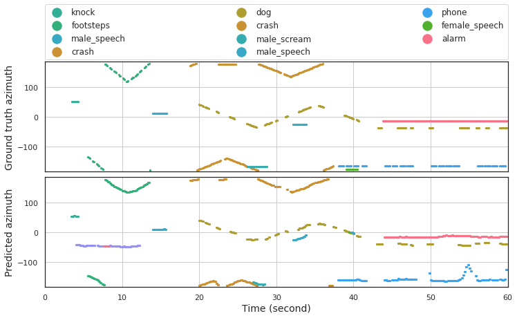
Figure 5: Visualization of ground truth and predicted azimuth for test clip fold6_room2_mix041 of the TNSSE 2021 dataset. Legend lists the ground truth events in chronological order. Sound classes are color-coded. piano event (purple) and an alarm event (pink) were misclassified between the $4$^th and the $12$^th seconds

Fig. 5 shows the plots of ground truth and predicted azimuth angles for a audio clip from the test set of the TNSSE 2021 dataset. The angles were predicted by a CRNN model trained on FOA SALSA features. Overall, the trajectories of predicted events were smooth and followed the ground truths closely. The model was able to correctly detect the sound classes and estimate DOAs across different numbers of overlapping sound sources (up to three overlapping sources). An unknown interference was misclassified as a piano event (purple) and an alarm event (pink) between the $4$th and the $12$th seconds. Since we used the class-wise output format to train the model, when there were two overlapping crash events between the $22$nd and the $24$th seconds, the model only predicted one crash event.

VII Conclusion

In conclusion, we proposed a novel and effective feature for polyphonic SELD named Spatial cue-Augmented Log-SpectrogrAm (SALSA), which consists of multichannel log-spectrograms and normalized principal eigenvector of the spatial covariance matrix at each TF bin of the spectrograms. There are two key characteristics that contribute to the effectiveness of the proposed feature. Firstly, SALSA spectrotemporally aligns the signal power and the source directional cues, which aids in resolving overlapping sound sources. This locally linear alignment works well with CNNs, where the filters learn the multichannel local pattern of the image-like input features. Secondly, SALSA includes helpful directional cues extracted from the principal eigenvectors of the spatial covariance matrices. Depending on the array type, where the directional cues might be encoded as interchannel amplitude and/or phase differences, the principal eigenvectors can be easily normalized to extract these cues. Therefore, SALSA features are versatile to use with different microphone array formats, such as FOA and MIC.

The proposed SALSA features can be further enhanced by incorporating signal processing-based methods such as magnitude and coherence tests to select more reliable directional cues and improve SELD performance. In addition, for multichannel arrays, spatial aliasing has little effect on the performance of models trained on SALSA. More importantly, the training segment length must be sufficient long for the model to capture the temporal dependency in the data.

In addition, data augmentation techniques such as channel swapping, frequency shifting, and random cutout can be readily applied to SALSA on the fly during training. These data augmentation techniques mitigated the problem of small datasets and significantly improved the performance of models trained on SALSA features. Simple CRNN models trained on the SALSA features achieved similar or even better SELD performance than many state-of-the-art systems on the TNSSE 2020 and 2021 datasets.

References

- [1] J. Salamon and J. P. Bello, “Deep Convolutional Neural Networks and Data Augmentation for Environmental Sound Classification,” IEEE Signal Processing Letters, vol. 24, no. 3, pp. 279–283, 2017.
- [2] D. Stowell, M. Wood, Y. Stylianou, and H. Glotin, “Bird detection in audio: A survey and a challenge,” in Proc. IEEE International Workshop Machine Learning Signal Processing, 2016.
- [3] P. Foggia, N. Petkov, A. Saggese, N. Strisciuglio, and M. Vento, “Audio Surveillance of Roads: A System for Detecting Anomalous Sounds,” IEEE Trans. Intelligent Transportation Systems, vol. 17, no. 1, pp. 279–288, 2016.
- [4] J. M. Valin, F. Michaud, B. Hadjou, and J. Rouat, “Localization of simultaneous moving sound sources for mobile robot using a frequency-domain steered beamformer approach,” in Proc. IEEE International Conference Robotics Automation, 2004, pp. 1033–1038.
- [5] S. Adavanne, A. Politis, J. Nikunen, and T. Virtanen, “Sound Event Localization and Detection of Overlapping Sources Using Convolutional Recurrent Neural Networks,” IEEE J. Selected Topics Signal Processing, vol. 13, no. 1, pp. 34–48, 2019.
- [6] T. Hirvonen, “Classification of spatial audio location and content using Convolutional neural networks,” in Proc. 138th Audio Engineering Society Conv. , 2015, pp. 622–631.
- [7] Y. Cao, Q. Kong, T. Iqbal, F. An, W. Wang, and M. D. Plumbley, “Polyphonic Sound Event Detection and Localization using a Two-Stage Strategy,” in Proc. 4th Workshop Detection Classification Acoustic Scenes Events, 2019.
- [8] L. Mazzon, Y. Koizumi, M. Yasuda, and N. Harada, “First Order Ambisonics Domain Spatial Augmentation for DNN-based Direction of Arrival Estimation,” in Proc. 4th Workshop Detection Classification Acoustic Scenes Events, 2019, pp. 154–158.
- [9] T. N. T. Nguyen, D. L. Jones, and W. Gan, “A Sequence Matching Network for Polyphonic Sound Event Localization and Detection,” in Proc. IEEE International Conference Acoustics, Speech Signal Processing, 2020, pp. 71–75.
- [10] T. N. T. Nguyen, N. K. Nguyen, H. Phan, L. Pham, K. Ooi, D. L. Jones, and W.-S. Gan, “A General Network Architecture for Sound Event Localization and Detection Using Transfer Learning and Recurrent Neural Network,” in Proc. IEEE International Conference Acoustics, Speech Signal Processing, 2021, pp. 935–939.
- [11] Y. Cao, T. Iqbal, Q. Kong, Y. Zhong, W. Wang, and M. D. Plumbley, “Event-independent Network for Polyphonic Sound Event Localization and Detection,” in Proc. 5th Workshop Detection Classification Acoustic Scenes Events, 2020.
- [12] Y. Cao, T. Iqbal, Q. Kong, F. An, W. Wang, and M. D. Plumbley, “An Improved Event-Independent Network for Polyphonic Sound Event Localization and Detection,” in Proc. IEEE International Conference Acoustics, Speech Signal Processing, 2021, pp. 885–889.
- [13] R. Sato, K. Niwa, and K. Kobayashi, “Ambisonic Signal Processing DNNs Guaranteeing Rotation, Scale and Time Translation Equivariance,” IEEE/ACM Trans. Audio Speech Language Processing, vol. 29, pp. 1449–1462, 2021.
- [14] H. Phan, L. Pham, P. Koch, N. Q. K. Duong, I. Mcloughlin, and A. Mertins, “On Multitask Loss Function for Audio Event Detection and Localization,” in Proc. 5th Workshop Detection Classification Acoustic Scenes Events, 2020.
- [15] Q. Wang, J. Du, H.-X. Wu, J. Pan, F. Ma, and C.-H. Lee, “A Four-Stage Data Augmentation Approach to ResNet-Conformer Based Acoustic Modeling for Sound Event Localization and Detection,”