Universal construction of decoders from encoding black boxes

Satoshi Yoshida Email: satoshi.yoshida@phys.s.u-tokyo.ac.jp Affiliation: Department of Physics, Graduate School of Science, The University of Tokyo, Hongo 7-3-1, Bunkyo-ku, Tokyo 113-0033, Japan OrcID: 0000-0002-0521-5209    Akihito Soeda Affiliation: Department of Physics, Graduate School of Science, The University of Tokyo, Hongo 7-3-1, Bunkyo-ku, Tokyo 113-0033, Japan Affiliation: Principles of Informatics Research Division, National Institute of Informatics, 2-1-2 Hitotsubashi, Chiyoda-ku, Tokyo 101-8430, Japan Affiliation: Department of Informatics, School of Multidisciplinary Sciences, SOKENDAI (The Graduate University for Advanced Studies), 2-1-2 Hitotsubashi, Chiyoda-ku, Tokyo 101-8430, Japan OrcID: 0000-0002-7502-5582    Mio Murao Affiliation: Department of Physics, Graduate School of Science, The University of Tokyo, Hongo 7-3-1, Bunkyo-ku, Tokyo 113-0033, Japan Affiliation: Trans-scale Quantum Science Institute, The University of Tokyo, Bunkyo-ku, Tokyo 113-0033, Japan OrcID: 0000-0001-7861-1774
Abstract

Isometry operations encode the quantum information of the input system to a larger output system, while the corresponding decoding operation would be an inverse operation of the encoding isometry operation. Given an encoding operation as a black box from a dd-dimensional system to a DD-dimensional system, we propose a universal protocol for isometry inversion that constructs a decoder from multiple calls of the encoding operation. This is a probabilistic but exact protocol whose success probability is independent of DD. For a qubit (d=2d=2) encoded in nn qubits, our protocol achieves an exponential improvement over any tomography-based or unitary-embedding method, which cannot avoid DD-dependence. We present a quantum operation that converts multiple parallel calls of any given isometry operation to random parallelized unitary operations, each of dimension dd. Applied to our setup, it universally compresses the encoded quantum information to a DD-independent space, while keeping the initial quantum information intact. This compressing operation is combined with a unitary inversion protocol to complete the isometry inversion. We also discover a fundamental difference between our isometry inversion protocol and the known unitary inversion protocols by analyzing isometry complex conjugation and isometry transposition. General protocols including indefinite causal order are searched using semidefinite programming for any improvement in the success probability over the parallel protocols. We find a sequential “success-or-draw” protocol of universal isometry inversion for d=2d=2 and D=3D=3, thus whose success probability exponentially improves over parallel protocols in the number of calls of the input isometry operation for the said case.

1 Introduction

Universal transformations of quantum states have played an essential role in the fundamental understanding of quantum information theory and its applications [1]. Recently, higher-order quantum transformations, namely, universal transformations of quantum operations given as black boxes, have been studied in the contexts of processing unitary operations [2, 3, 4, 5, 6, 7, 8, 9, 10, 11, 12, 13, 14, 15, 16, 17, 18, 19, 20, 21, 22, 23, 24], non-Markovian quantum process [25, 26, 27, 28, 29, 30, 31, 32, 33, 34, 35, 36, 37], and dynamical resource theory [38, 39, 40, 41, 42, 43, 44, 45, 46, 47, 48, 49, 50, 51, 52]. They can also be interpreted as quantum functional programming [53, 54]. The concept of higher-order quantum transformation was initially introduced as single-input quantum supermaps [55], and a multiple-input version was introduced as quantum combs [56], which are realizable by quantum circuits with a fixed ordering of input operations. A similar concept was studied as channels with memory [57] and quantum strategies [58].

In particular, higher-order quantum transformations of unitary operations have been extensively studied for aiming to utilize in quantum information processing (e.g., estimation of group transformations [2], quantum learning of unitary operations [3, 4, 5, 6], cloning of unitary operations [7, 8, 9, 10, 11, 12], process tomography [13, 14], unitary complex conjugation [15], unitary inversion [16, 17, 18, 19, 20] and unitary controllization [22, 23, 24]). Isometry operations are also frequently used in quantum protocols, as they preserve information of the input state similarly to unitary operations. For instance, encoding of quantum information is represented by an isometry operation [1]. In addition, many quantum algorithms use fixed auxiliary states and such algorithms can also be considered to be utilizing isometry operations (e.g., Harrow-Hassidim-Lloyd (HHL) algorithm [59]). Despite their importance, higher-order quantum transformations of isometry operations are not well investigated yet.

In this work, we study one of the fundamental higher-order quantum transformation tasks for isometry operations, namely, isometry inversion. Isometry inversion is a task to implement the inverse map of an input isometry operation, interpreted as retrieving quantum information encoded by the isometry operation. Such a retrieval of quantum information is widely studied in the context of quantum error correction [1], quantum secret sharing [60], quantum communication [61], and uncomputation [62, 63]. Such studies usually assume that the complete descriptions of encoding operations are given. Contrary, this work considers a universal protocol without knowing the descriptions except for the dimensions of the input system and the output system. The universal protocol implements the inverse operation probabilistically but exactly.

The special case of probabilistic exact isometry inversion, namely probabilistic exact unitary inversion [18, 19], is known. This implementation relies on the existence of two protocols: (deterministic exact) unitary complex conjugation [15] and (probabilistic exact) unitary transposition [19]. However, this strategy is not directly applicable for isometry inversion. The key idea for unitary complex conjugation protocol presented in Ref. [15] is to utilize the knowledge of representation theory of the unitary group, but this idea cannot be applied to isometry complex conjugation since the set of isometry operations does not form a group. In fact, we show below a no-go theorem for isometry complex conjugation.

The most trivial way to implement isometry inversion in the black box setting is to obtain a classical description of the isometry operation by quantum process tomography [1] and then implement the inverse map based on the description, namely, using the “measure-and-prepare” strategy [64, 3]. However, known quantum process tomography protocols [65] require a DD-dependent number of experiments to obtain an approximate description of an isometry operation 𝒱~d,D\widetilde{\mathcal{V}}_{d,D} from a dd-dimensional system to a DD-dimensional system (see the discussion in Section 3.4). Another straightforward way is to embed an isometry operation 𝒱~d,D\widetilde{\mathcal{V}}_{d,D} in a DD-dimensional unitary operation and then apply a universal probabilistic exact unitary inversion protocol [18]. However, the success probability of such a protocol cannot avoid the dependence on DD, either. In particular, for isometry operations encoding quantum information of a qudit (a dd-dimensional system) into nn qudits (a dnd^{n}-dimensional system), the exponential cost in nn due to the dimensionality of D=dnD=d^{n} may seem to be inevitable for implementing isometry inversion.

Nevertheless, we present a probabilistic but exact protocol for isometry inversion of which success probability does not depend on DD. Due to this property, our protocol can significantly outperform the protocols based on the two strategies mentioned above. To compare with the protocol based on unitary inversion, we consider an isometry operation that encodes a qubit into five qubits, i.e., d=2d=2 and D=25D=2^{5}. The unitary inversion requires at least D1=31D-1=31 calls to obtain a non-zero success probability [18], but our protocol achieves a success probability p=87%p=87\% by 2020 calls. Compared with the protocol based on quantum process tomography, our protocol can implement isometry inversion approximately within a fixed error ϵ\epsilon by a DD-independent number of calls. This comparison exhibits the potential power of a higher-order quantum transformation that directly transforms a black box operation without evaluating its classical description.

We also clarify a crucial difference between the unitary inversion protocols presented in Ref. [18] and the isometry inversion protocol. Reference [18] presents a systematic construction of unitary inversion protocols concatenating unitary transposition [19] and unitary complex conjugation [15]. The unitary complex conjugation protocol utilizes the fact that the complex conjugate representation of the unitary group is unitarily equivalent to the antisymmetric subspace of the tensor representation of the unitary group [15]. The unitary transposition protocol presented in Ref. [19] uses a variant of the gate teleportation [66] or the probabilistic port-based teleportation [67, 68]. However, we show that isometry inversion cannot be implemented by concatenating the corresponding tasks since no probabilistic exact isometry complex conjugation is possible for D2dD\geq 2d. We also show that any isometry inversion protocol transposing a “pseudo complex conjugate” map (see Section 4.2) of an isometry operation by a variant of gate teleportation [66] is less efficient than our protocol.

The key idea of our isometry inversion protocol is a quantum operation that universally compresses the DD-dimensional output spaces of the isometry operations into dd-dimensional quantum systems. We first extend the irreducible decomposition of the tensor product of unitary operators known as the Schur-Weyl duality to isometry operators. We show that the tensor product of isometry operators also admits a block diagonal decomposition, despite the isometry operators not forming a group. This decomposition identifies relevant and irrelevant components to retrieve quantum information encoded by the isometry operation. The compressing quantum operation discards the irrelevant component. We utilize the compressing quantum operation to convert unitary inversion protocols to isometry inversion protocols avoiding the DD-dependence of the success probability and the no-go theorem for isometry complex conjugation.

Our isometry inversion protocol uses input operations in parallel. Such parallel protocols form an essential class of higher-order quantum transformation because parallelization is a common technique to reduce the circuit depth [69]. However, more general protocols than parallel ones can be helpful to improve the success probability. In this work, we consider sequential protocols using input operations in a fixed ordering and general protocols including indefinite causal order [70, 71, 72, 73, 74, 75, 76] in addition to parallel ones. To see the performance improvement in our setting, we conduct semidefinite programming (SDP) to obtain the optimal success probability of parallel, sequential, and general protocols.

The rest of this paper is organized as follows. Section 2 states the problem setting for implementing isometry transposition, isometry complex conjugation, and isometry inversion. Section 3 presents the main result of this paper, constructing a parallel protocol for isometry inversion by investigating the compressing quantum operation. Section 4 discusses the difference between our isometry inversion protocol and the previous work on unitary inversion. Section 5 shows numerical results on the optimal success probability of parallel, sequential, and general protocols including indefinite causal order for isometry inversion, isometry (pseudo) complex conjugation, and isometry transposition. Section 6 concludes the paper.

2 Problem Setting

2.1 Inverse maps of isometry operations

A dd-dimensional quantum system is represented by a Hilbert space =d\mathcal{H}=\mathbb{C}^{d} and a state of the system is represented by a density operator (a positive semi-definite operator with unit trace) ρ\rho on \mathcal{H}. A state is called pure if its density operator has rank 1, i.e., ρ=|ψψ|\rho=|{\psi}\rangle\!\langle{\psi}| for |ψ|{\psi}\rangle\in\mathcal{H}. The set of linear operators on \mathcal{H} is denoted by ()\mathcal{L}(\mathcal{H}) and the set of linear operators from \mathcal{H} to \mathcal{H^{\prime}} is denoted by ()\mathcal{L}(\mathcal{H}\to\mathcal{H}^{\prime}). When we explicitly specify the dimension of the set of linear operators, we denote the corresponding sets by (d)\mathcal{L}(\mathbb{C}^{d}) and (dD)\mathcal{L}(\mathbb{C}^{d}\to\mathbb{C}^{D}), respectively, for =d\mathcal{H}=\mathbb{C}^{d} and =d\mathcal{H}^{\prime}=\mathbb{C}^{d}. We only consider quantum systems represented by finite-dimensional Hilbert spaces in this paper.

An isometry operation transforms a pure input state in a dd-dimensional system =d\mathcal{H}=\mathbb{C}^{d} to a pure output state in a DD-dimensional system =D\mathcal{H}^{\prime}=\mathbb{C}^{D} with DdD\geq d where the transformation preserves the inner product of two input states. An isometry operation is regarded to encode (and spread for the case of d<Dd<D) quantum information represented by a dd-dimensional quantum state into a DD-dimensional state. Unitary operations are special cases of isometry operations with d=Dd=D.

Formally, an isometry operation 𝒱~:()()\widetilde{\mathcal{V}}:\mathcal{L}(\mathcal{H})\to\mathcal{L}(\mathcal{H}^{\prime}) for =d\mathcal{H}=\mathbb{C}^{d} and =D\mathcal{H}^{\prime}=\mathbb{C}^{D} is a completely positive trace preserving (CPTP) map given as 𝒱~(ρ)=VρV\widetilde{\mathcal{V}}(\rho)=V\rho V^{\dagger} in terms of an isometry operator V:V:\mathcal{H}\to\mathcal{H}^{\prime}, an element of the set of isometry operators 𝕍iso(d,D)\mathbb{V}_{\mathrm{iso}}(d,D) defined by

𝕍iso(d,D)\displaystyle\mathbb{V}_{\mathrm{iso}}(d,D) {V(dD)|VV=𝟙d},\displaystyle\coloneqq\{V\in\mathcal{L}{(\mathbb{C}^{d}\to\mathbb{C}^{D})}|V^{\dagger}V=\mathds{1}_{d}\}, (1)

where 𝟙d\mathds{1}_{d} is the identity operator on =d\mathcal{H}=\mathbb{C}^{d}, and V:V^{\dagger}:\mathcal{H}^{\prime}\to\mathcal{H} is the adjoint of VV. In this notation, the tilde symbol on top of 𝒱\mathcal{V} represents a linear map11 1 This convention is adopted from Ref. [19].. We denote a set of dd-dimensional unitary operators by 𝕌(d)\mathbb{U}(d), which is equivalent to 𝕍iso(d,d)\mathbb{V}_{\mathrm{iso}}(d,d), and a unitary operation corresponding to a unitary operator UU by 𝒰~\widetilde{\mathcal{U}}.

We define the most general map which can decode the states encoded by an isometry operation 𝒱~\widetilde{\mathcal{V}}. We consider a completely positive (CP) map 𝒱~inv:()()\widetilde{\mathcal{V}}_{\mathrm{inv}}:\mathcal{L}(\mathcal{H}^{\prime})\to\mathcal{L}(\mathcal{H}) that satisfies

𝒱~inv𝒱~=𝟙~d,\displaystyle\widetilde{\mathcal{V}}_{\mathrm{inv}}\circ\widetilde{\mathcal{V}}=\widetilde{\mathds{1}}_{d}, (2)

for an isometry operation 𝒱~\widetilde{\mathcal{V}} corresponding to V𝕍iso(d,D)V\in\mathbb{V}_{\mathrm{iso}}(d,D), where 𝟙~d\widetilde{\mathds{1}}_{d} is the identity operation on ()\mathcal{L}(\mathcal{H}), which is defined by 𝟙~d(ρ)=ρ\widetilde{\mathds{1}}_{d}(\rho)=\rho for all density matrices ρ\rho of a dd-dimensional system. We refer to a map 𝒱~inv\widetilde{\mathcal{V}}_{\mathrm{inv}} satisfying Eq. (2) as an inverse map of 𝒱~\widetilde{\mathcal{V}}. Note that 𝒱~inv\widetilde{\mathcal{V}}_{\mathrm{inv}} is not necessarily a trace preserving map, while the composition of 𝒱~inv\widetilde{\mathcal{V}}_{\mathrm{inv}} and 𝒱~\widetilde{\mathcal{V}} is trace preserving. An inverse map is not necessarily the adjoint map 𝒱~\widetilde{\mathcal{V}}^{\dagger} defined as 𝒱~(ρ)=VρV\widetilde{\mathcal{V}}^{\dagger}(\rho)=V^{\dagger}\rho V, either. For instance, a CP map 𝒱~α\widetilde{\mathcal{V}}^{\prime}_{\alpha} defined by

𝒱~α(ρ)VρV+αIddTr[Π(ImV)ρ]\displaystyle\widetilde{\mathcal{V}}^{\prime}_{\alpha}(\rho)\coloneqq V^{\dagger}\rho V+\alpha\frac{I_{d}}{d}{\mathrm{Tr}}\left[\Pi_{({\mathrm{Im}}V)^{\perp}}\rho\right] (3)

is also an inverse map of 𝒱~\widetilde{\mathcal{V}} for α0\alpha\geq 0, where Π(ImV)\Pi_{({\mathrm{Im}}V)^{\perp}} is a projector onto the orthogonal subspace of the image of V:V:\mathcal{H}\to\mathcal{H^{\prime}} denoted by ImVV(){\mathrm{Im}}V\coloneqq V(\mathcal{H}). The map 𝒱~α\widetilde{\mathcal{V}}^{\prime}_{\alpha} is not trace preserving for α1\alpha\neq 1, but the composition of 𝒱~\widetilde{\mathcal{V}} and 𝒱~α\widetilde{\mathcal{V}}^{\prime}_{\alpha} is trace preserving because the second term of Eq. (3) vanishes for all ρ(ImV)\rho\in\mathcal{L}({\mathrm{Im}}V).

2.2 Higher-order quantum transformations of isometry operations: parallel protocols for probabilistic exact tasks

In this paper, we present a probabilistic but universal and exact protocol to construct an inverse map 𝒱~inv\widetilde{\mathcal{V}}_{\mathrm{inv}} from finite calls of an unknown isometry operation 𝒱~\widetilde{\mathcal{V}} given as a black box. Such a protocol can be regarded as implementing a higher-order quantum transformation of an isometry operation, similarly to the preceding works considered higher-order quantum transformations of a unitary operation [18, 19], of which formulation is based on the notion of quantum supermaps and superinstrument [55].

We first introduce the notations of quantum supermaps [55] describing higher-order deterministic quantum transformations. A quantum supermap is a linear completely CPTP preserving transformation from an input map to an output map. We consider a kk-input supermap 𝒞~~{\mathchoice{\widetilde{\hbox{$\displaystyle\widetilde{\mathcal{C}}$}}}{\widetilde{\hbox{$\textstyle\widetilde{\mathcal{C}}$}}}{\widetilde{\hbox{$\scriptstyle\widetilde{\mathcal{C}}$}}}{\widetilde{\hbox{$\scriptscriptstyle\widetilde{\mathcal{C}}$}}}} that transforms kk input maps Λ~in(i):(i)(𝒪i)\widetilde{\Lambda}^{(i)}_{\mathrm{in}}:\mathcal{L}(\mathcal{I}_{i})\to\mathcal{L}(\mathcal{O}_{i}) for i{1,,k}i\in\{1,\cdots,k\}, where i\mathcal{I}_{i} and 𝒪i\mathcal{O}_{i} represent the input Hilbert space and the output Hilbert space of the ii-th input map Λ~in(i)\widetilde{\Lambda}^{(i)}_{\mathrm{in}}, respectively, to an output map Λ~out:(𝒫)()\widetilde{\Lambda}_{\mathrm{out}}:\mathcal{L}(\mathcal{P})\to\mathcal{L}(\mathcal{F}), where 𝒫\mathcal{P} and \mathcal{F} represent the input Hilbert space (also referred to as the past space) and the output Hilbert space (also referred to as the future space), respectively, of Λ~out\widetilde{\Lambda}_{\mathrm{out}}. The double tilde symbol on top of 𝒞\mathcal{C} represents a linear supermap (or a linear superinstrument, which will be introduced in the next paragraph)22 2 This convention is also adopted from Ref. [19]..
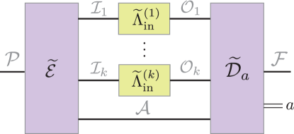
Figure 1: A quantum circuit representation of a parallel superinstrument {𝒞~~a}\{{\mathchoice{\widetilde{\hbox{$\displaystyle\widetilde{\mathcal{C}}$}}}{\widetilde{\hbox{$\textstyle\widetilde{\mathcal{C}}$}}}{\widetilde{\hbox{$\scriptstyle\widetilde{\mathcal{C}}$}}}{\widetilde{\hbox{$\scriptscriptstyle\widetilde{\mathcal{C}}$}}}}_{a}\} defined in Eq. (4), where Λ~in(i)(i{1,,k})\widetilde{\Lambda}_{\mathrm{in}}^{(i)}\;(i\in\{1,\cdots,k\}) are input maps, ~\widetilde{\mathcal{E}} is a CPTP map, and {𝒟~a}\{\widetilde{\mathcal{D}}_{a}\} is a quantum instrument. A wire corresponds to a Hilbert space and a box corresponds to an operation. The double line in this figure represents the classical outcome of the measurement.

Since we mainly focus on probabilistic parallel protocols, we introduce the notions of a parallel superinstrument representing a higher-order probabilistic quantum transformation where all input maps are called in parallel [19]. For a parallel protocol, it is convenient to define the joint input Hilbert space i=1ki\mathcal{I}\coloneqq\bigotimes_{i=1}^{k}\mathcal{I}_{i} and the joint output Hilbert space as 𝒪i=1k𝒪i\mathcal{O}\coloneqq\bigotimes_{i=1}^{k}\mathcal{O}_{i}, as well as the joint input map Λ~ini=1kΛ~in(i)\widetilde{\Lambda}_{\mathrm{in}}\coloneqq\bigotimes_{i=1}^{k}\widetilde{\Lambda}^{(i)}_{\mathrm{in}}. Using these notations, a parallel superinstrument is a set of kk-input supermaps {𝒞~~a}:[()(𝒪)][(𝒫)()]\{{\mathchoice{\widetilde{\hbox{$\displaystyle\widetilde{\mathcal{C}}$}}}{\widetilde{\hbox{$\textstyle\widetilde{\mathcal{C}}$}}}{\widetilde{\hbox{$\scriptstyle\widetilde{\mathcal{C}}$}}}{\widetilde{\hbox{$\scriptscriptstyle\widetilde{\mathcal{C}}$}}}}_{a}\}:[\mathcal{L}(\mathcal{I})\to\mathcal{L}(\mathcal{O})]\to[\mathcal{L}(\mathcal{P})\to\mathcal{L}(\mathcal{F})] given by

𝒞~~a(Λ~in)=𝒟~a(Λ~in𝟙~𝒜)~,\displaystyle{\mathchoice{\widetilde{\hbox{$\displaystyle\widetilde{\mathcal{C}}$}}}{\widetilde{\hbox{$\textstyle\widetilde{\mathcal{C}}$}}}{\widetilde{\hbox{$\scriptstyle\widetilde{\mathcal{C}}$}}}{\widetilde{\hbox{$\scriptscriptstyle\widetilde{\mathcal{C}}$}}}}_{a}(\widetilde{\Lambda}_{\mathrm{in}})=\widetilde{\mathcal{D}}_{a}\circ\left(\widetilde{\Lambda}_{\mathrm{in}}\otimes\widetilde{\mathds{1}}_{\mathcal{A}}\right)\circ\widetilde{\mathcal{E}}, (4)

where ~:(𝒫)(𝒜)\widetilde{\mathcal{E}}:\mathcal{L}(\mathcal{P})\to\mathcal{L}(\mathcal{I}\otimes\mathcal{A}) is a CPTP map, {𝒟~a}:(𝒪𝒜)()\{\widetilde{\mathcal{D}}_{a}\}:\mathcal{L}(\mathcal{O}\otimes\mathcal{A})\to\mathcal{L}(\mathcal{F}) is a quantum instrument33 3 A quantum instrument {Ψ~a}\{\widetilde{\Psi}_{a}\} is a set of CP maps such that aΨ~a\sum_{a}\widetilde{\Psi}_{a} is a CPTP map [61]. and 𝒜\mathcal{A} is an auxiliary Hilbert space (see Figure 1). We note that a parallel protocol using kk copies of an input isometry operation does not require the kk copies to be available simultaneously during the protocol. We may substitute by using a single black box isometry operation repeatedly kk times.

This work also considers constructions of probabilistic exact parallel protocols for the complex conjugate map and the transposition map of an isometry operation to compare the protocol with that of unitary inversion. For this sake, we introduce a notation of general higher-order probabilistic quantum transformation of an isometry operation 𝒱~\widetilde{\mathcal{V}} to another map which is a function of 𝒱~\widetilde{\mathcal{V}} denoted as f(V)~\widetilde{f(V)} 44 4 We write the argument of the function ff as VV instead of 𝒱~\widetilde{\mathcal{V}} to avoid a duplicate use of a tilde.. Note that the function ff is not necessarily linear in terms of a single 𝒱~\widetilde{\mathcal{V}} , but has to be linear in terms of 𝒱~k\widetilde{\mathcal{V}}^{\otimes k}, and not necessary to be trace preserving either.

A probabilistic exact parallel protocol of a higher-order quantum transformation of kk calls of an unknown isometry operation 𝒱~\widetilde{\mathcal{V}} to f(V)~\widetilde{f(V)} is formulated as follows. Let {𝒮~~,~~}:[()(𝒪)][(𝒫)()]\{{\mathchoice{\widetilde{\hbox{$\displaystyle\widetilde{\mathcal{S}}$}}}{\widetilde{\hbox{$\textstyle\widetilde{\mathcal{S}}$}}}{\widetilde{\hbox{$\scriptstyle\widetilde{\mathcal{S}}$}}}{\widetilde{\hbox{$\scriptscriptstyle\widetilde{\mathcal{S}}$}}}},{\mathchoice{\widetilde{\hbox{$\displaystyle\widetilde{\mathcal{F}}$}}}{\widetilde{\hbox{$\textstyle\widetilde{\mathcal{F}}$}}}{\widetilde{\hbox{$\scriptstyle\widetilde{\mathcal{F}}$}}}{\widetilde{\hbox{$\scriptscriptstyle\widetilde{\mathcal{F}}$}}}}\}:[\mathcal{L}(\mathcal{I})\to\mathcal{L}(\mathcal{O})]\to[\mathcal{L}(\mathcal{P})\to\mathcal{L}(\mathcal{F}{)]} be a parallel superinstrument, where 𝒮~~{\mathchoice{\widetilde{\hbox{$\displaystyle\widetilde{\mathcal{S}}$}}}{\widetilde{\hbox{$\textstyle\widetilde{\mathcal{S}}$}}}{\widetilde{\hbox{$\scriptstyle\widetilde{\mathcal{S}}$}}}{\widetilde{\hbox{$\scriptscriptstyle\widetilde{\mathcal{S}}$}}}} denotes the successful transformation and ~~{\mathchoice{\widetilde{\hbox{$\displaystyle\widetilde{\mathcal{F}}$}}}{\widetilde{\hbox{$\textstyle\widetilde{\mathcal{F}}$}}}{\widetilde{\hbox{$\scriptstyle\widetilde{\mathcal{F}}$}}}{\widetilde{\hbox{$\scriptscriptstyle\widetilde{\mathcal{F}}$}}}} denotes the failure transformation. We say that a parallel protocol 𝒮~~{\mathchoice{\widetilde{\hbox{$\displaystyle\widetilde{\mathcal{S}}$}}}{\widetilde{\hbox{$\textstyle\widetilde{\mathcal{S}}$}}}{\widetilde{\hbox{$\scriptstyle\widetilde{\mathcal{S}}$}}}{\widetilde{\hbox{$\scriptscriptstyle\widetilde{\mathcal{S}}$}}}} is a probabilistic exact protocol to implement f(V)~\widetilde{f(V)} from kk calls of 𝒱~\widetilde{\mathcal{V}} if

𝒮~~(𝒱~k)=psuccf(V)~(V𝕍iso(d,D))\displaystyle{\mathchoice{\widetilde{\hbox{$\displaystyle\widetilde{\mathcal{S}}$}}}{\widetilde{\hbox{$\textstyle\widetilde{\mathcal{S}}$}}}{\widetilde{\hbox{$\scriptstyle\widetilde{\mathcal{S}}$}}}{\widetilde{\hbox{$\scriptscriptstyle\widetilde{\mathcal{S}}$}}}}(\widetilde{\mathcal{V}}^{\otimes k})=p_{\mathrm{succ}}\widetilde{f(V)}\;\;\;(\forall V\in\mathbb{V}_{\mathrm{iso}}(d,D)) (5)

holds. We require that psuccp_{\mathrm{succ}} is independent of the input isometry operation 𝒱~\widetilde{\mathcal{V}} and the input quantum state ρin\rho_{\mathrm{in}}, and call it the success probability of f(V)~\widetilde{f(V)} for the following reasons. Note that the probability to obtain the successful measurement outcome is psuccTr[f(V)~(ρin)]p_{\text{succ}}{\mathrm{Tr}}[\widetilde{f(V)}(\rho_{\mathrm{in}})], where ρin\rho_{\mathrm{in}} is the input state. The probability to obtain the successful measurement can be divided into two terms; one is the success probability of the protocol denoted by psuccp_{\text{succ}}, and the other is the success probability of the map f(V)~\widetilde{f(V)} denoted by Tr[f(V)~(ρin)]{\mathrm{Tr}}[\widetilde{f(V)}(\rho_{\mathrm{in}})]. For the case of f(V)~=𝒱~inv\widetilde{f(V)}=\widetilde{\mathcal{V}}_{\mathrm{inv}} (isometry inversion), psuccp_{\mathrm{succ}} coincides with the probability to obtain the successful measurement outcome when the input quantum state is in the image Im𝒱~{\mathrm{Im}}\widetilde{\mathcal{V}}, since 𝒱~inv𝒱~\widetilde{\mathcal{V}}_{\mathrm{inv}}\circ\widetilde{\mathcal{V}} is trace preserving. Then, the success probability psuccp_{\mathrm{succ}} for isometry inversion represents the probability to obtain the quantum state ρ\rho when the input state is 𝒱~(ρ)\widetilde{\mathcal{V}}(\rho).

We summarize a list of f(V)~\widetilde{f(V)} discussed in this paper. Isometry inversion (1) is the main topic of this work, and other tasks (2, 3, 4) are analyzed to compare isometry inversion with the previous works [19, 18] on unitary inversion.

  1. 1.

    Isometry inversion: f(V)~=𝒱~inv,\widetilde{f(V)}=\widetilde{\mathcal{V}}_{\mathrm{inv}},
    such that 𝒱~inv𝒱~=𝟙~d\widetilde{\mathcal{V}}_{\mathrm{inv}}\circ\widetilde{\mathcal{V}}=\widetilde{\mathds{1}}_{d}.

  2. 2.

    Isometry complex conjugation: f(V)~=𝒱~,\widetilde{f(V)}=\widetilde{\mathcal{V}}^{*},
    where 𝒱~(ρ)=Vρ(V)\widetilde{\mathcal{V}}^{*}(\rho)=V^{*}\rho(V^{*})^{\dagger}. Here, VV^{*} denotes the complex conjugate of VV in the computational basis.

  3. 3.

    Isometry pseudo complex conjugation (see Section 4.2): f(V)~=𝒱~pcc,\widetilde{f(V)}=\widetilde{\mathcal{V}}_{\mathrm{pcc}},
    such that 𝒱~pccT𝒱~=𝟙~d\widetilde{\mathcal{V}}_{\mathrm{pcc}}^{T}\circ\widetilde{\mathcal{V}}=\widetilde{\mathds{1}}_{d}, where the transposed map Λ~T\widetilde{\Lambda}^{T} for a CP map Λ~\widetilde{\Lambda} given by its action as Λ~(ρ)=kKkρKk\widetilde{\Lambda}(\rho)=\sum_{k}K_{k}\rho K_{k}^{\dagger} in terms of the Kraus operators {Kk}\{K_{k}\} is defined as Λ~T(ρ)kKkTρ(KkT)\widetilde{\Lambda}^{T}(\rho)\coloneqq\sum_{k}K_{k}^{T}\rho(K_{k}^{T})^{\dagger}.

  4. 4.

    Isometry transposition: f(V)~=𝒱~T,\widetilde{f(V)}=\widetilde{\mathcal{V}}^{T},
    where 𝒱~T(ρ)=VTρ(VT)\widetilde{\mathcal{V}}^{T}(\rho)=V^{T}\rho(V^{T})^{\dagger}. Here, VTV^{T} denotes the transpose of VV in the computational basis.

In quantum circuits shown in the figures in the rest of the paper, we sometimes write V𝕍iso(d,D)V\in\mathbb{V}_{\mathrm{iso}}(d,D) as Vd,DV_{d,D} to represent the dimensions of its input and output Hilbert spaces explicitly in quantum circuits. To illustrate the dimensions of the Hilbert spaces represented by the wires of quantum circuits in the figures, we use the following color coding of wires: a red wire corresponds to a dd-dimensional Hilbert space, a blue wire corresponds to a DD-dimensional Hilbert space, and a black wire corresponds to a Hilbert space with an arbitrary dimension. The dual lines in the quantum circuits represent classical information transmissions.

3 The parallel isometry inversion protocol

3.1 Main result: Parallel isometry inversion with DD-independent success probability

We present our main theorem on the optimal success probability of the probabilistic exact parallel protocol for isometry inversion. The success probability only depends on the dimension of the input Hilbert space of the isometry, and thus significantly outperforms the probabilistic exact parallel protocols based on unitary inversion (see Figure 6 (b)).

Theorem 1.

The optimal success probability of probabilistic parallel protocols that transform kk calls of an isometry operation 𝒱~:(d)(D)\widetilde{\mathcal{V}}:\mathcal{L}(\mathbb{C}^{d})\to\mathcal{L}(\mathbb{C}^{D}) into its inverse map 𝒱~inv\widetilde{\mathcal{V}}_{\mathrm{inv}} does not depend on DD. Moreover, a parallel protocol shown in Figure 2 (a) achieves a success probability psucc=k/(d1)/[d2+k/(d1)1]p_{\mathrm{succ}}=\lfloor k/(d-1)\rfloor/[d^{2}+\lfloor k/(d-1)\rfloor-1], which is optimal for d=2d=2.

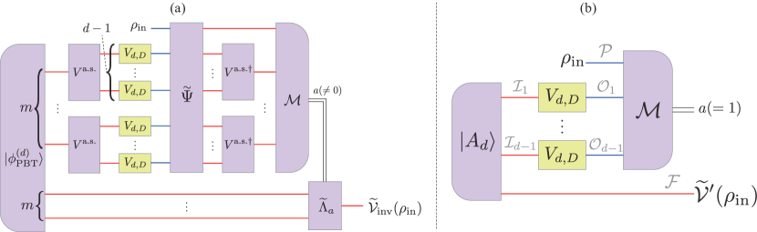
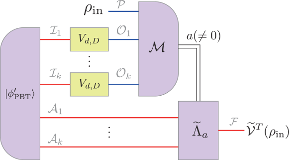
Before proceeding the proof of Theorem 1 and showing the detail of the protocol shown in Figure 2 (a), we show how an isometry inversion protocol is implemented in the case of k=d1k=d-1 calls, as the protocol is shown by a quantum circuit represented in Figure 2 (b). In the quantum circuit, |Ad=(d)d|{A_{d}}\rangle\in\mathcal{I}\otimes\mathcal{F}=(\mathbb{C}^{d})^{\otimes d} is the totally antisymmetric state defined by

|Adj{1,,d}dϵjd!|j1j2jd,\displaystyle|{A_{d}}\rangle\coloneqq\sum_{\vec{j}\in\{1,\cdots,d\}^{d}}\frac{\epsilon_{\vec{j}}}{\sqrt{d!}}|{j_{1}j_{2}\cdots j_{d}}\rangle, (6)

where {|ji}(i=1,,d)\{|{j_{i}}\rangle\}\;(i=1,\cdots,d) is an orthonormal basis of d\mathbb{C}^{d} and ϵj\epsilon_{\vec{j}} is the antisymmetric tensor with rank dd. The POVM \mathcal{M} is a projective measurement {Π1=Πa.s.,Π0=I𝒫𝒪Πa.s.}\{\Pi_{1}=\Pi^{\mathrm{a.s.}},\Pi_{0}=I_{\mathcal{P}\mathcal{O}}-\Pi^{\mathrm{a.s.}}\}, where Πa.s.\Pi^{\mathrm{a.s.}} is the orthogonal projector on 𝒫𝒪1𝒪d1=(D)d\mathcal{P}\otimes\mathcal{O}_{1}\otimes\cdots\otimes\mathcal{O}_{d-1}=(\mathbb{C}^{D})^{\otimes d} onto the subspace spanned by the totally antisymmetric states. This protocol succeeds when the measurement outcome of ={Πa}\mathcal{M}=\{\Pi_{a}\} is a=1a=1. This quantum circuit implements an isometry inversion protocol as shown in the following theorem. See Appendix G for the proof.

Theorem 2.

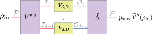
A parallel protocol shown in Figure 2 (b) transforms d1d-1 calls of an isometry operation 𝒱~\widetilde{\mathcal{V}} corresponding to V𝕍iso(d,D)V\in\mathbb{V}_{\mathrm{iso}}(d,D) into its inverse map 𝒱~inv\widetilde{\mathcal{V}}_{\mathrm{inv}} with a success probability psucc=1/d2p_{\mathrm{succ}}=1/d^{2}. Moreover, this protocol implements the inverse map 𝒱~inv=𝒱~\widetilde{\mathcal{V}}_{\mathrm{inv}}=\widetilde{\mathcal{V}}^{\prime} given by

𝒱~(ρin)VρinV+𝟙dTr[Π(ImV)ρin],\displaystyle\widetilde{\mathcal{V}}^{\prime}(\rho_{\mathrm{in}})\coloneqq V^{\dagger}\rho_{\mathrm{in}}V+\mathds{1}_{d}{\mathrm{Tr}}\left[\Pi_{({\mathrm{Im}}V)^{\perp}}\rho_{\mathrm{in}}\right], (7)

where Π(ImV)\Pi_{({\mathrm{Im}}V)^{\perp}} is the orthogonal projector onto the orthogonal complement (ImV)({\mathrm{Im}}V)^{\perp} of ImVD{\mathrm{Im}}V\subset\mathbb{C}^{D}.

Figure 2: (a) A quantum circuit representation of a parallel delayed input-state protocol for isometry inversion that achieves the success probability psucc=k/(d1)/[d2+k/(d1)1]p_{\mathrm{succ}}=\lfloor k/(d-1)\rfloor/[d^{2}+\lfloor k/(d-1)\rfloor-1]. In the quantum circuit, m(d1)m(d-1) calls of the input isometry operation 𝒱~d,D\widetilde{\mathcal{V}}_{d,D} for m=k/(d1)m=\lfloor k/(d-1)\rfloor are used, and the rest km(d1)k-m(d-1) calls of 𝒱~d,D\widetilde{\mathcal{V}}_{d,D} are discarded (not shown in the figure). The CPTP map Ψ~\widetilde{\Psi} is defined in Eq. (22). The quantum state |ϕPBT(d)|{\phi^{(d)}_{\mathrm{PBT}}}\rangle and the POVM ={Γa(d)}a=0k\mathcal{M}=\{\Gamma_{a}^{(d)}\}_{a=0}^{k} are the optimal resource state and the POVM for the probabilistic port-based teleportation [67, 68], which are defined in Eqs. (100) and (101), respectively. The conditional CPTP map Λ~a\widetilde{\Lambda}_{a} is the post-processing operation used in port-based teleportation defined in Eq. (111), which selects the quantum state in 𝒜a\mathcal{A}_{a} corresponding to the measurement outcome aa of \mathcal{M} as the output state for a0a\neq 0. The isometry operator Va.s.V^{\mathrm{a.s.}} represents an encoding of quantum information on a totally antisymmetric state defined in Eq. (62). This protocol succeeds when the measurement outcome aa is a0a\neq 0. (b) The isometry inversion protocol shown in (a) reduces to the circuit shown in this figure for m=1m=1, i.e., k=d1k=d-1. The quantum state |Ad|{A_{d}}\rangle is the totally antisymmetric state defined in Eq. (6) and the POVM \mathcal{M} is a projective measurement {Π1=Πa.s.,Π0=𝟙𝒫𝒪Πa.s.}\{\Pi_{1}=\Pi^{\mathrm{a.s.}},\Pi_{0}=\mathds{1}_{\mathcal{P}\mathcal{O}}-\Pi^{\mathrm{a.s.}}\}, where Πa.s.\Pi^{\mathrm{a.s.}} is the orthogonal projector on 𝒫𝒪1𝒪d1=(D)d\mathcal{P}\otimes\mathcal{O}_{1}\otimes\cdots\otimes\mathcal{O}_{d-1}=(\mathbb{C}^{D})^{\otimes d} onto the subspace spanned by the totally antisymmetric states. This protocol implements the inverse map 𝒱~inv=𝒱~\widetilde{\mathcal{V}}_{\mathrm{inv}}=\widetilde{\mathcal{V}}^{\prime} of VV defined in Eq. (7) when the measurement outcome of ={Πa}\mathcal{M}=\{\Pi_{a}\} is a=1a=1.

Theorem 2 states the existence of a parallel isometry inversion protocol whose success probability does not depend on DD for k=d1k=d-1. Now, we go back to Theorem 1, which is a generalization of Theorem 2. The first part of Theorem 1 states the DD-independence of the optimal success probability of parallel isometry inversion. In general, an isometry operation V𝕍iso(d,D)V\in\mathbb{V}_{\mathrm{iso}}(d,D^{\prime}) can be embedded in 𝕍iso(d,D)\mathbb{V}_{\mathrm{iso}}(d,D) for DDdD\geq D^{\prime}\geq d. Using this embedding, we can show the optimal success probability of parallel isometry inversion using kk calls of the input isometry operation V𝕍iso(d,D)V\in\mathbb{V}_{\mathrm{iso}}(d,D), denoted by popt(d,D,k)p_{\mathrm{opt}}(d,D,k), is monotonically non-increasing in the output dimension DD of VV, i.e.,

popt(d,D,k)popt(d,D,k)\displaystyle p_{\mathrm{opt}}(d,D^{\prime},k)\geq p_{\mathrm{opt}}(d,D,k) (8)

holds for all dd, kk, DD, and DD^{\prime} such that DDdD\geq D^{\prime}\geq d. We present a proof of this statement for D=dD^{\prime}=d in the proof of Theorem 1 (see Figure 5 (b)) and a similar construction is possible for any DDdD\geq D^{\prime}\geq d. Thus, it is enough to show the converse of Eq. (8) given by

popt(d,d,k)popt(d,D,k).\displaystyle p_{\mathrm{opt}}(d,d,k)\leq p_{\mathrm{opt}}(d,D,k). (9)

We show this relation by constructing a CPTP map compressing the output space of isometry operations to dd-dimensional spaces. Using this CPTP map, we show the construction of a parallel isometry inversion protocol of V𝕍iso(d,D)V\in\mathbb{V}_{\mathrm{iso}}(d,D) from a corresponding parallel unitary inversion protocol of U𝕌(d)(=𝕍iso(d,d))U\in\mathbb{U}(d)(=\mathbb{V}_{\mathrm{iso}}(d,d)). The second part shows the series of parallel isometry inversion protocols with DD-independent success probability approaching 1 for kk\to\infty. This asymptotic behavior is natural since one can perform the process tomography of V𝕍iso(d,D)V\in\mathbb{V}_{\text{iso}}(d,D) to construct the inverse operation deterministically for kk\to\infty. We note that the optimality of the success probability shown in Theorem 1 is still open since the optimal parallel protocol for unitary inversion is not analytically known except for the case of d=2d=2.

3.2 Construction of isometry inversion protocol from a given parallel delayed-input state protocol for unitary inversion

We consider a subclass of parallel protocols to proceed the proof of Theorem 1. We say that a superinstrument is realized by a parallel delayed input-state protocol if an input state is inserted after applying black box operations similarly to the one given by the quantum circuit shown in Figure 2 (a) (see Ref. [19] for the detail). As shown in the following Lemma, an isometry inversion protocol can be constructed from a given parallel delayed-input state protocol for unitary inversion.

Since the input quantum state in the Hilbert space 𝒫\mathcal{P} and the output state of 𝒱~d,Dk\widetilde{\mathcal{V}}_{d,D}^{\otimes k} in the Hilbert space 𝒪=i=1k𝒪i\mathcal{O}=\bigotimes_{i=1}^{k}\mathcal{O}_{i} are available at some point of the parallel delayed input-state protocol, we can apply a CPTP map Ψ~\widetilde{\Psi} on 𝒫𝒪\mathcal{P}\otimes\mathcal{O}. Using this idea, we construct an isometry inversion protocol (see the proof of Lemma 3). Note that this construction is not valid for a general (i.e., non delayed input-state) parallel protocol since the input quantum state in the Hilbert space 𝒫\mathcal{P} is not available after applying the input isometry operation (see Figure 1).

Lemma 3.

Suppose we are given a parallel delayed input-state protocol that transforms kk calls of a unitary operation 𝒰~:(d)(d)\widetilde{\mathcal{U}}:\mathcal{L}(\mathbb{C}^{d})\to\mathcal{L}(\mathbb{C}^{d}) into its inverse map 𝒰~\widetilde{\mathcal{U}}^{\dagger} with a success probability psucc{p^{\prime}_{\mathrm{succ}}}. Then, we can construct a parallel delayed input-state protocol that transforms kk calls of an isometry operation 𝒱~:(d)(D)\widetilde{\mathcal{V}}:\mathcal{L}(\mathbb{C}^{d})\to\mathcal{L}(\mathbb{C}^{D}) into its inverse map 𝒱~inv\widetilde{\mathcal{V}}_{\mathrm{inv}} with the same success probability psucc=psuccp_{\mathrm{succ}}={p^{\prime}_{\mathrm{succ}}}.

Proof.

We construct a CPTP map Ψ~\widetilde{\Psi} transforming k+1k+1 parallel calls of isometry V𝕍iso(d,D)V\in\mathbb{V}_{\text{iso}}(d,D) into parallel calls of a random unitary U𝕌(d)U\in\mathbb{U}(d) (see Eq. (23)). This CPTP map Ψ~\widetilde{\Psi} compresses the output state of isometry operations on dd-dimensional systems keeping the relevant component to retrieve the input state, which contributes to the DD- independence of the success probability. Then, we construct an isometry inversion protocol by inserting the CPTP map Ψ~\widetilde{\Psi} into a given unitary inversion protocol (see Figure 5 (a)). In the following, we derive Ψ~\widetilde{\Psi} and show the protocol and the achievability of psuccp_{\mathrm{succ}}.

We first introduce a parallel delayed input-state kk-input superinstrument {𝒮~~,~~}:[()(𝒪)][(𝒫)()]\{{\mathchoice{\widetilde{\hbox{$\displaystyle\widetilde{\mathcal{S}^{\prime}}$}}}{\widetilde{\hbox{$\textstyle\widetilde{\mathcal{S}^{\prime}}$}}}{\widetilde{\hbox{$\scriptstyle\widetilde{\mathcal{S}^{\prime}}$}}}{\widetilde{\hbox{$\scriptscriptstyle\widetilde{\mathcal{S}^{\prime}}$}}}},{\mathchoice{\widetilde{\hbox{$\displaystyle\widetilde{\mathcal{F}^{\prime}}$}}}{\widetilde{\hbox{$\textstyle\widetilde{\mathcal{F}^{\prime}}$}}}{\widetilde{\hbox{$\scriptstyle\widetilde{\mathcal{F}^{\prime}}$}}}{\widetilde{\hbox{$\scriptscriptstyle\widetilde{\mathcal{F}^{\prime}}$}}}}\}:[\mathcal{L}(\mathcal{I})\to\mathcal{L}(\mathcal{O}^{\prime})]\to[\mathcal{L}(\mathcal{P}^{\prime})\to\mathcal{L}(\mathcal{F})] defined by

𝒮~~(Λ~in)()\displaystyle{\mathchoice{\widetilde{\hbox{$\displaystyle\widetilde{\mathcal{S}^{\prime}}$}}}{\widetilde{\hbox{$\textstyle\widetilde{\mathcal{S}^{\prime}}$}}}{\widetilde{\hbox{$\scriptstyle\widetilde{\mathcal{S}^{\prime}}$}}}{\widetilde{\hbox{$\scriptscriptstyle\widetilde{\mathcal{S}^{\prime}}$}}}}(\widetilde{\Lambda}_{\mathrm{in}})(\cdot) =[𝒟~S(𝟙~𝒫Λ~in𝟙~𝒜)](ϕ𝒜),\displaystyle=\left[\widetilde{\mathcal{D}}^{\prime}_{S}\circ\left(\widetilde{\mathds{1}}_{\mathcal{P}^{\prime}}\otimes\widetilde{\Lambda}_{\mathrm{in}}\otimes\widetilde{\mathds{1}}_{\mathcal{A}}\right)\right](\cdot\otimes{\phi^{\prime}}_{\mathcal{IA}}), (10)
~~(Λ~in)()\displaystyle{\mathchoice{\widetilde{\hbox{$\displaystyle\widetilde{\mathcal{F}^{\prime}}$}}}{\widetilde{\hbox{$\textstyle\widetilde{\mathcal{F}^{\prime}}$}}}{\widetilde{\hbox{$\scriptstyle\widetilde{\mathcal{F}^{\prime}}$}}}{\widetilde{\hbox{$\scriptscriptstyle\widetilde{\mathcal{F}^{\prime}}$}}}}(\widetilde{\Lambda}_{\mathrm{in}})(\cdot) =[𝒟~F(𝟙~𝒫Λ~in𝟙~𝒜)](ϕ𝒜),\displaystyle=\left[{\widetilde{\mathcal{D}}^{\prime}_{F}}\circ\left(\widetilde{\mathds{1}}_{\mathcal{P}^{\prime}}\otimes\widetilde{\Lambda}_{\mathrm{in}}\otimes\widetilde{\mathds{1}}_{\mathcal{A}}\right)\right](\cdot\otimes{\phi^{\prime}}_{\mathcal{IA}}), (11)

where the joint Hilbert space are defined by i=1ki\mathcal{I}\coloneqq\bigotimes_{i=1}^{k}\mathcal{I}_{i} and 𝒪i=1k𝒪i\mathcal{O}^{\prime}\coloneqq\bigotimes_{i=1}^{k}\mathcal{O}^{\prime}_{i}, 𝒜\mathcal{A} is an auxiliary system, ϕ𝒜(𝒜){\phi^{\prime}}_{\mathcal{IA}}\in\mathcal{L}(\mathcal{I}\otimes\mathcal{A}) is a quantum state and {𝒟~S,𝒟~F}:(𝒫𝒪𝒜)()\{{{\widetilde{\mathcal{D}}^{\prime}_{S},\widetilde{\mathcal{D}}^{\prime}_{F}}}\}:\mathcal{L}(\mathcal{P}^{\prime}\otimes\mathcal{O}^{\prime}\otimes\mathcal{A})\to\mathcal{L}(\mathcal{F}) is a quantum instrument (see the left panel of Figure 5 (a)). Note that a prime is added on the quantum state ϕ\phi^{\prime}, the quantum instrument {𝒟~S,𝒟~F}\{{{\widetilde{\mathcal{D}}^{\prime}_{S},\widetilde{\mathcal{D}}^{\prime}_{F}}}\}, and the Hilbert spaces 𝒪i\mathcal{O}_{i}^{\prime} and 𝒫\mathcal{P}^{\prime} to distinguish {𝒮~~,~~}\{{\mathchoice{\widetilde{\hbox{$\displaystyle\widetilde{\mathcal{S}^{\prime}}$}}}{\widetilde{\hbox{$\textstyle\widetilde{\mathcal{S}^{\prime}}$}}}{\widetilde{\hbox{$\scriptstyle\widetilde{\mathcal{S}^{\prime}}$}}}{\widetilde{\hbox{$\scriptscriptstyle\widetilde{\mathcal{S}^{\prime}}$}}}},{\mathchoice{\widetilde{\hbox{$\displaystyle\widetilde{\mathcal{F}^{\prime}}$}}}{\widetilde{\hbox{$\textstyle\widetilde{\mathcal{F}^{\prime}}$}}}{\widetilde{\hbox{$\scriptstyle\widetilde{\mathcal{F}^{\prime}}$}}}{\widetilde{\hbox{$\scriptscriptstyle\widetilde{\mathcal{F}^{\prime}}$}}}}\} from another superinstrument {𝒮~~,~~}\{{\mathchoice{\widetilde{\hbox{$\displaystyle\widetilde{\mathcal{S}}$}}}{\widetilde{\hbox{$\textstyle\widetilde{\mathcal{S}}$}}}{\widetilde{\hbox{$\scriptstyle\widetilde{\mathcal{S}}$}}}{\widetilde{\hbox{$\scriptscriptstyle\widetilde{\mathcal{S}}$}}}},{\mathchoice{\widetilde{\hbox{$\displaystyle\widetilde{\mathcal{F}}$}}}{\widetilde{\hbox{$\textstyle\widetilde{\mathcal{F}}$}}}{\widetilde{\hbox{$\scriptstyle\widetilde{\mathcal{F}}$}}}{\widetilde{\hbox{$\scriptscriptstyle\widetilde{\mathcal{F}}$}}}}\} defined later (see Eqs. (13) and (14)). Suppose 𝒫=d\mathcal{P}^{\prime}=\mathbb{C}^{d}, =d\mathcal{F}=\mathbb{C}^{d}, i=d\mathcal{I}_{i}=\mathbb{C}^{d} and 𝒪i=d\mathcal{O}^{\prime}_{i}=\mathbb{C}^{d} for i{1,,k}i\in\{1,\cdots,k\}. We assume that the superinstrument {𝒮~~,~~}\{{\mathchoice{\widetilde{\hbox{$\displaystyle\widetilde{\mathcal{S}^{\prime}}$}}}{\widetilde{\hbox{$\textstyle\widetilde{\mathcal{S}^{\prime}}$}}}{\widetilde{\hbox{$\scriptstyle\widetilde{\mathcal{S}^{\prime}}$}}}{\widetilde{\hbox{$\scriptscriptstyle\widetilde{\mathcal{S}^{\prime}}$}}}},{\mathchoice{\widetilde{\hbox{$\displaystyle\widetilde{\mathcal{F}^{\prime}}$}}}{\widetilde{\hbox{$\textstyle\widetilde{\mathcal{F}^{\prime}}$}}}{\widetilde{\hbox{$\scriptstyle\widetilde{\mathcal{F}^{\prime}}$}}}{\widetilde{\hbox{$\scriptscriptstyle\widetilde{\mathcal{F}^{\prime}}$}}}}\} implements unitary inversion with a success probability psucc{p^{\prime}_{\mathrm{succ}}}, i.e.,

𝒮~~(𝒰~k)=psucc𝒰~(U𝕌(d)).\displaystyle{\mathchoice{\widetilde{\hbox{$\displaystyle\widetilde{\mathcal{S}^{\prime}}$}}}{\widetilde{\hbox{$\textstyle\widetilde{\mathcal{S}^{\prime}}$}}}{\widetilde{\hbox{$\scriptstyle\widetilde{\mathcal{S}^{\prime}}$}}}{\widetilde{\hbox{$\scriptscriptstyle\widetilde{\mathcal{S}^{\prime}}$}}}}(\widetilde{\mathcal{U}}^{\otimes k})={p^{\prime}_{\mathrm{succ}}}\;\widetilde{\mathcal{U}}^{\dagger}\;\;\;(\forall U\in\mathbb{U}(d)). (12)

Next, we consider the condition that a parallel delayed input-state superinstrument {𝒮~~,~~}\{{\mathchoice{\widetilde{\hbox{$\displaystyle\widetilde{\mathcal{S}}$}}}{\widetilde{\hbox{$\textstyle\widetilde{\mathcal{S}}$}}}{\widetilde{\hbox{$\scriptstyle\widetilde{\mathcal{S}}$}}}{\widetilde{\hbox{$\scriptscriptstyle\widetilde{\mathcal{S}}$}}}},{\mathchoice{\widetilde{\hbox{$\displaystyle\widetilde{\mathcal{F}}$}}}{\widetilde{\hbox{$\textstyle\widetilde{\mathcal{F}}$}}}{\widetilde{\hbox{$\scriptstyle\widetilde{\mathcal{F}}$}}}{\widetilde{\hbox{$\scriptscriptstyle\widetilde{\mathcal{F}}$}}}}\} implements isometry inversion. Suppose 𝒫=d\mathcal{P}=\mathbb{C}^{d} and 𝒪i=D\mathcal{O}_{i}=\mathbb{C}^{D} for i{1,,k}i\in\{1,\cdots,k\} and define the joint Hilbert space by 𝒪i=1k𝒪i\mathcal{O}\coloneqq\bigotimes_{i=1}^{k}\mathcal{O}_{i}. We consider a parallel delayed input-state superinstrument {𝒮~~,~~}:[()(𝒪)][(𝒫)()]\{{\mathchoice{\widetilde{\hbox{$\displaystyle\widetilde{\mathcal{S}}$}}}{\widetilde{\hbox{$\textstyle\widetilde{\mathcal{S}}$}}}{\widetilde{\hbox{$\scriptstyle\widetilde{\mathcal{S}}$}}}{\widetilde{\hbox{$\scriptscriptstyle\widetilde{\mathcal{S}}$}}}},{\mathchoice{\widetilde{\hbox{$\displaystyle\widetilde{\mathcal{F}}$}}}{\widetilde{\hbox{$\textstyle\widetilde{\mathcal{F}}$}}}{\widetilde{\hbox{$\scriptstyle\widetilde{\mathcal{F}}$}}}{\widetilde{\hbox{$\scriptscriptstyle\widetilde{\mathcal{F}}$}}}}\}:[\mathcal{L}(\mathcal{I})\to\mathcal{L}(\mathcal{O})]\to[\mathcal{L}(\mathcal{P})\to\mathcal{L}(\mathcal{F})] given by

𝒮~~(Λ~in)()\displaystyle{\mathchoice{\widetilde{\hbox{$\displaystyle\widetilde{\mathcal{S}}$}}}{\widetilde{\hbox{$\textstyle\widetilde{\mathcal{S}}$}}}{\widetilde{\hbox{$\scriptstyle\widetilde{\mathcal{S}}$}}}{\widetilde{\hbox{$\scriptscriptstyle\widetilde{\mathcal{S}}$}}}}(\widetilde{\Lambda}_{\mathrm{in}})(\cdot) =[𝒟~S(𝟙~𝒫Λ~in𝟙~𝒜)](ϕ𝒜),\displaystyle=\left[{\widetilde{\mathcal{D}}_{S}}\circ\left(\widetilde{\mathds{1}}_{\mathcal{P}}\otimes\widetilde{\Lambda}_{\mathrm{in}}\otimes\widetilde{\mathds{1}}_{\mathcal{A}}\right)\right](\cdot\otimes\phi_{\mathcal{IA}}), (13)
~~(Λ~in)()\displaystyle{\mathchoice{\widetilde{\hbox{$\displaystyle\widetilde{\mathcal{F}}$}}}{\widetilde{\hbox{$\textstyle\widetilde{\mathcal{F}}$}}}{\widetilde{\hbox{$\scriptstyle\widetilde{\mathcal{F}}$}}}{\widetilde{\hbox{$\scriptscriptstyle\widetilde{\mathcal{F}}$}}}}(\widetilde{\Lambda}_{\mathrm{in}})(\cdot) =[𝒟~F(𝟙~𝒫Λ~in𝟙~𝒜)](ϕ𝒜),\displaystyle=\left[{\widetilde{\mathcal{D}}_{F}}\circ\left(\widetilde{\mathds{1}}_{\mathcal{P}}\otimes\widetilde{\Lambda}_{\mathrm{in}}\otimes\widetilde{\mathds{1}}_{\mathcal{A}}\right)\right](\cdot\otimes\phi_{\mathcal{IA}}), (14)

where 𝒜\mathcal{A} is an auxiliary system, ϕ𝒜(𝒜)\phi_{\mathcal{IA}}\in\mathcal{L}(\mathcal{I}\otimes\mathcal{A}) is a quantum state and {𝒟~S,𝒟~F}:(𝒫𝒪𝒜)()\{{{\widetilde{\mathcal{D}}_{S},\widetilde{\mathcal{D}}_{F}}}\}:\mathcal{L}(\mathcal{P}\otimes\mathcal{O}\otimes\mathcal{A})\to\mathcal{L}(\mathcal{F}) is a quantum instrument (see the left panel of Figure 3). The condition that superinstrument {𝒮~~,~~}\{{\mathchoice{\widetilde{\hbox{$\displaystyle\widetilde{\mathcal{S}}$}}}{\widetilde{\hbox{$\textstyle\widetilde{\mathcal{S}}$}}}{\widetilde{\hbox{$\scriptstyle\widetilde{\mathcal{S}}$}}}{\widetilde{\hbox{$\scriptscriptstyle\widetilde{\mathcal{S}}$}}}},{\mathchoice{\widetilde{\hbox{$\displaystyle\widetilde{\mathcal{F}}$}}}{\widetilde{\hbox{$\textstyle\widetilde{\mathcal{F}}$}}}{\widetilde{\hbox{$\scriptstyle\widetilde{\mathcal{F}}$}}}{\widetilde{\hbox{$\scriptscriptstyle\widetilde{\mathcal{F}}$}}}}\} implements isometry inversion with the success probability psuccp_{\mathrm{succ}} is given by

𝒮~~(𝒱~)=psucc𝒱~inv(V𝕍iso(d,D)).\displaystyle{\mathchoice{\widetilde{\hbox{$\displaystyle\widetilde{\mathcal{S}}$}}}{\widetilde{\hbox{$\textstyle\widetilde{\mathcal{S}}$}}}{\widetilde{\hbox{$\scriptstyle\widetilde{\mathcal{S}}$}}}{\widetilde{\hbox{$\scriptscriptstyle\widetilde{\mathcal{S}}$}}}}(\widetilde{\mathcal{V}})=p_{\mathrm{succ}}\widetilde{\mathcal{V}}_{\mathrm{inv}}\;\;\;(\forall V\in\mathbb{V}_{\mathrm{iso}}(d,D)). (15)

By definition of the inverse map 𝒱~inv\widetilde{\mathcal{V}}_{\mathrm{inv}}, this condition is equivalent to the condition given by

𝒮~~(𝒱~)𝒱~=psucc𝟙~d,\displaystyle{\mathchoice{\widetilde{\hbox{$\displaystyle\widetilde{\mathcal{S}}$}}}{\widetilde{\hbox{$\textstyle\widetilde{\mathcal{S}}$}}}{\widetilde{\hbox{$\scriptstyle\widetilde{\mathcal{S}}$}}}{\widetilde{\hbox{$\scriptscriptstyle\widetilde{\mathcal{S}}$}}}}(\widetilde{\mathcal{V}})\circ\widetilde{\mathcal{V}}=p_{\mathrm{succ}}\widetilde{\mathds{1}}_{d}, (16)

i.e.,

[𝒟~S(𝒱~𝒫′′𝒫𝒪k+1𝟙~𝒜)](ρ𝒫′′ϕ𝒜)=psuccρ\displaystyle\left[{\widetilde{\mathcal{D}}_{S}}\circ\left(\widetilde{\mathcal{V}}^{\otimes k+1}_{\mathcal{P}^{\prime\prime}\mathcal{I}\to\mathcal{P}\mathcal{O}}\otimes\widetilde{\mathds{1}}_{\mathcal{A}}\right)\right](\rho_{\mathcal{P}^{\prime\prime}}\otimes\phi_{\mathcal{IA}})=p_{\mathrm{succ}}\rho_{\mathcal{F}} (17)

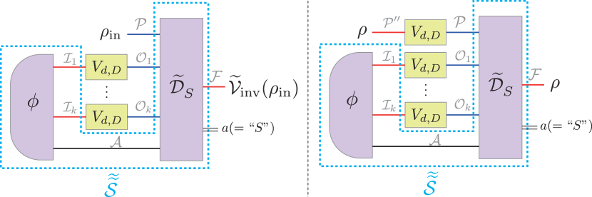
for all V𝕍iso(d,D)V\in\mathbb{V}_{\mathrm{iso}}(d,D) and ρ(𝒫′′)\rho\in\mathcal{L}(\mathcal{P}^{\prime\prime}) (see the right panel of Figure 3). Here, the Hilbert space 𝒫′′\mathcal{P}^{\prime\prime} is given by 𝒫′′=d\mathcal{P}^{\prime\prime}=\mathbb{C}^{d}. This condition means that we have to retrieve the quantum state ρ\rho after applying the tensor product of an isometry operation 𝒱~k+1\widetilde{\mathcal{V}}^{\otimes k+1}.

Figure 3: Left panel: A quantum circuit representation of a parallel delayed input-state protocol {𝒮~~,~~}\{{\mathchoice{\widetilde{\hbox{$\displaystyle\widetilde{\mathcal{S}}$}}}{\widetilde{\hbox{$\textstyle\widetilde{\mathcal{S}}$}}}{\widetilde{\hbox{$\scriptstyle\widetilde{\mathcal{S}}$}}}{\widetilde{\hbox{$\scriptscriptstyle\widetilde{\mathcal{S}}$}}}},{\mathchoice{\widetilde{\hbox{$\displaystyle\widetilde{\mathcal{F}}$}}}{\widetilde{\hbox{$\textstyle\widetilde{\mathcal{F}}$}}}{\widetilde{\hbox{$\scriptstyle\widetilde{\mathcal{F}}$}}}{\widetilde{\hbox{$\scriptscriptstyle\widetilde{\mathcal{F}}$}}}}\}. This protocol succeeds when the successful measurement outcome is obtained (a=Sa=\text{``}S\text{''}). Right panel: The condition that the parallel delayed input-state protocol {𝒮~~,~~}\{{\mathchoice{\widetilde{\hbox{$\displaystyle\widetilde{\mathcal{S}}$}}}{\widetilde{\hbox{$\textstyle\widetilde{\mathcal{S}}$}}}{\widetilde{\hbox{$\scriptstyle\widetilde{\mathcal{S}}$}}}{\widetilde{\hbox{$\scriptscriptstyle\widetilde{\mathcal{S}}$}}}},{\mathchoice{\widetilde{\hbox{$\displaystyle\widetilde{\mathcal{F}}$}}}{\widetilde{\hbox{$\textstyle\widetilde{\mathcal{F}}$}}}{\widetilde{\hbox{$\scriptstyle\widetilde{\mathcal{F}}$}}}{\widetilde{\hbox{$\scriptscriptstyle\widetilde{\mathcal{F}}$}}}}\} shown in the left panel implements isometry inversion with the success probability psuccp_{\mathrm{succ}} is equivalent to the condition that the output state of the quantum circuit shown in the right panel retrieves the input state ρ\rho with the success probability psuccp_{\mathrm{succ}}. This protocol succeeds when the successful measurement outcome is obtained (a=Sa=\text{``}S\text{''}).

We show the decomposition of the tensor product Vk+1V^{\otimes k+1} of an isometry operator VV to consider how to retrieve the quantum state ρ\rho after the application of Vk+1V^{\otimes k+1}. The joint Hilbert spaces 𝒫′′=(d)k+1\mathcal{P}^{\prime\prime}\otimes\mathcal{I}=(\mathbb{C}^{d})^{\otimes k+1}, 𝒫𝒪=(d)k+1\mathcal{P}^{\prime}\otimes\mathcal{O}^{\prime}=(\mathbb{C}^{d})^{\otimes k+1} and 𝒫𝒪=(D)k+1\mathcal{P}\otimes\mathcal{O}=(\mathbb{C}^{D})^{\otimes k+1} can be decomposed as

𝒫′′\displaystyle{\mathcal{P}^{\prime\prime}\otimes\mathcal{I}} =μk+1𝒰μ,𝒫′′(d)𝒮μ,𝒫′′(k+1),\displaystyle={\bigoplus_{\mu\vdash k+1}\mathcal{U}_{\mu,\mathcal{P}^{\prime\prime}\mathcal{I}}^{(d)}\otimes\mathcal{S}_{\mu,\mathcal{P}^{\prime\prime}\mathcal{I}}^{(k+1)},} (18)
𝒫𝒪\displaystyle\mathcal{P}^{\prime}\otimes\mathcal{O}^{\prime} =μk+1𝒰μ,𝒫𝒪(d)𝒮μ,𝒫𝒪(k+1),\displaystyle=\bigoplus_{\mu\vdash k+1}\mathcal{U}_{\mu,\mathcal{P}^{\prime}\mathcal{O}^{\prime}}^{(d)}\otimes\mathcal{S}_{\mu,\mathcal{P}^{\prime}\mathcal{O}^{\prime}}^{(k+1)}, (19)
𝒫𝒪\displaystyle\mathcal{P}\otimes\mathcal{O} =μk+1𝒰μ,𝒫𝒪(D)𝒮μ,𝒫𝒪(k+1).\displaystyle=\bigoplus_{\mu\vdash k+1}\mathcal{U}_{\mu,\mathcal{P}\mathcal{O}}^{(D)}\otimes\mathcal{S}_{\mu,\mathcal{P}\mathcal{O}}^{(k+1)}. (20)

by the Schur-Weyl duality , where μ\mu is a Young diagram with k+1k+1 boxes, denoted by μk+1\mu\vdash k+1 (see Appendix B for the detail). Let {|μ,uμ,sμ}\{|{\mu,u_{\mu},s_{\mu}}\rangle\} be the orthonormal basis of 𝒰μ,𝒫𝒪(d)𝒮μ,𝒫𝒪(k+1)\mathcal{U}_{\mu,\mathcal{P}^{\prime}\mathcal{O}^{\prime}}^{(d)}\otimes\mathcal{S}_{\mu,\mathcal{P}^{\prime}\mathcal{O}^{\prime}}^{(k+1)} for each μ\mu and we call {|μ,uμ,sμ}\{|{\mu,u_{\mu},s_{\mu}}\rangle\} the Schur basis (see also Appendix B). We define the change of basis U𝒫𝒪SchU^{\mathrm{Sch}}_{\mathcal{P}^{\prime}\mathcal{O}^{\prime}} transforming the computational basis for 𝒫𝒪\mathcal{P}^{\prime}\otimes\mathcal{O}^{\prime} to the Schur basis, and suppose |μ|{\mu}\rangle, |uμ|{u_{\mu}}\rangle and |sμ|{s_{\mu}}\rangle are stored in the Hilbert spaces 𝒫𝒪\mathcal{M}_{\mathcal{P}^{\prime}\mathcal{O}^{\prime}}, 𝒰𝒫𝒪\mathcal{U}_{\mathcal{P}^{\prime}\mathcal{O}^{\prime}} and 𝒮𝒫𝒪\mathcal{S}_{\mathcal{P}^{\prime}\mathcal{O}^{\prime}}, respectively. The unitary operator U𝒫𝒪SchU^{\mathrm{Sch}}_{\mathcal{P}^{\prime}\mathcal{O}^{\prime}} is called the quantum Schur transform [77, 78, 79]. Using the decomposition of Hilbert spaces given by Eqs. (18) and (20), we can decompose the tensor product Vk+1:𝒫′′𝒫𝒪V^{\otimes k+1}:\mathcal{P}^{\prime\prime}\otimes\mathcal{I}\to\mathcal{P}\otimes\mathcal{O} of an isometry operator V𝕍iso(d,D)V\in\mathbb{V}_{\mathrm{iso}}(d,D) as

Vk+1=μk+1l(μ)dVμI𝒮μ,𝒫′′(k+1)𝒮μ,𝒫𝒪(k+1),\displaystyle V^{\otimes k+1}=\bigoplus_{\begin{subarray}{c}\mu\vdash k+1\\ l(\mu)\leq d\end{subarray}}V_{\mu}\otimes I_{\mathcal{S}_{\mu,\mathcal{P}^{\prime\prime}\mathcal{I}}^{(k+1)}\to\mathcal{S}_{\mu,\mathcal{P}\mathcal{O}}^{(k+1)}}, (21)

where l(μ)l(\mu) is the number of rows of a Young diagram μ\mu, Vμ(𝒰μ,𝒫′′(d)𝒰μ,𝒫𝒪(D))V_{\mu}\in\mathcal{L}(\mathcal{U}_{\mu,\mathcal{P}^{\prime\prime}\mathcal{I}}^{(d)}\to\mathcal{U}_{\mu,\mathcal{P}\mathcal{O}}^{(D)}) is an isometry operator depending on the isometry VV and I𝒮μ,𝒫′′(k+1)𝒮μ,𝒫𝒪(k+1)I_{\mathcal{S}_{\mu,\mathcal{P}^{\prime\prime}\mathcal{I}}^{(k+1)}\to\mathcal{S}_{\mu,\mathcal{PO}}^{(k+1)}} is the isomorphism between irreducible representations 𝒮μ,𝒫𝒪(k+1)\mathcal{S}_{\mu,\mathcal{P}^{\prime}\mathcal{O}^{\prime}}^{(k+1)} and 𝒮μ,𝒫𝒪(k+1)\mathcal{S}_{\mu,\mathcal{PO}}^{(k+1)}. We prove this decomposition in Appendix B (see Eq. (89)). This decomposition shows that the quantum information encoded in 𝒮μ,𝒫′′(k+1)\mathcal{S}^{(k+1)}_{\mu,\mathcal{P}^{\prime\prime}\mathcal{I}} is unchanged by the action of the parallel calls of any isometry operator V𝕍iso(d,D)V\in\mathbb{V}_{\mathrm{iso}}(d,D), while the quantum information encoded in 𝒰μ,𝒫′′(d)\mathcal{U}_{\mu,\mathcal{P}^{\prime\prime}\mathcal{I}}^{(d)} is affected by a VV-dependent action. In addition, the Hilbert space 𝒰μ,𝒫𝒪(D)𝒮μ,𝒫𝒪(k+1)\mathcal{U}_{\mu,\mathcal{P}\mathcal{O}}^{(D)}\otimes\mathcal{S}_{\mu,\mathcal{P}\mathcal{O}}^{(k+1)} for l(μ)>dl(\mu)>d is out of the image ImVk+1{\mathrm{Im}}V^{\otimes k+1}. From these observations, the quantum information relevant to retrieve the quantum state ρ\rho after the application of 𝒱~k+1\widetilde{\mathcal{V}}^{\otimes k+1} is considered to be encoded in the Hilbert space 𝒮μ,𝒫𝒪(k+1)\mathcal{S}_{\mu,\mathcal{P}\mathcal{O}}^{(k+1)} for l(μ)dl(\mu)\leq d. Then, we can “compress” the output state of 𝒱~k+1\widetilde{\mathcal{V}}^{\otimes k+1} to a smaller Hilbert space whose dimension is independent of DD by a CPTP map Ψ~\widetilde{\Psi} defined in the next paragraph.

We define a key element for constructing an isometry inversion protocol, a CPTP map Ψ~:(𝒫𝒪)(𝒫𝒪)\widetilde{\Psi}:\mathcal{L}(\mathcal{P}\otimes\mathcal{O})\to\mathcal{L}(\mathcal{P}^{\prime}\otimes\mathcal{O}^{\prime}), by

Ψ~𝒫𝒪𝒫𝒪(ρ)\displaystyle\widetilde{\Psi}_{\mathcal{P}\mathcal{O}\to\mathcal{P}^{\prime}\mathcal{O}^{\prime}}(\rho)
μk+1l(μ)d𝟙𝒰μ,𝒫𝒪(d)d𝒰μ(d)[~𝒮μ,𝒫𝒪(k+1)𝒮μ,𝒫𝒪(k+1)Tr𝒰μ,𝒫𝒪(D)(Πμ,𝒫𝒪ρ)]+𝟙𝒫𝒪d𝒫𝒪×μk+1l(μ)>dTr(Πμ,𝒫𝒪ρ),\displaystyle\coloneqq\bigoplus_{\begin{subarray}{c}\mu\vdash k+1\\ l(\mu)\leq d\end{subarray}}\frac{\mathds{1}_{\mathcal{U}^{(d)}_{\mu,\mathcal{P}^{\prime}\mathcal{O}^{\prime}}}}{d_{\mathcal{U}_{\mu}^{(d)}}}\otimes\left[\widetilde{\mathcal{I}}_{{\mathcal{S}^{(k+1)}_{\mu,\mathcal{PO}}\to\mathcal{S}^{(k+1)}_{\mu,\mathcal{P}^{\prime}\mathcal{O}^{\prime}}}}{\mathrm{Tr}}_{\mathcal{U}_{\mu,\mathcal{P}\mathcal{O}}^{(D)}}(\Pi_{\mu,\mathcal{PO}}\rho)\right]+\frac{\mathds{1}_{\mathcal{P}^{\prime}\mathcal{O}^{\prime}}}{d_{\mathcal{P}^{\prime}\mathcal{O}^{\prime}}}\times\sum_{\begin{subarray}{c}\mu\vdash k+1\\ l(\mu)>d\end{subarray}}{\mathrm{Tr}}(\Pi_{\mu,\mathcal{PO}}\rho), (22)

where Πμ,𝒫𝒪\Pi_{\mu,\mathcal{PO}} is a projector on the Hilbert space 𝒫𝒪\mathcal{P}\otimes\mathcal{O} onto its subspace 𝒰μ,𝒫𝒪(D)𝒮μ,𝒫𝒪(k+1)\mathcal{U}_{\mu,\mathcal{P}\mathcal{O}}^{(D)}\otimes\mathcal{S}_{\mu,\mathcal{P}\mathcal{O}}^{(k+1)}. The CPTP map Ψ~\widetilde{\Psi} “extracts” the quantum information encoded in 𝒮μ,𝒫𝒪(k+1)\mathcal{S}^{(k+1)}_{\mu,\mathcal{P}\mathcal{O}} for l(μ)dl(\mu)\leq d from 𝒫𝒪\mathcal{P}\otimes\mathcal{O} by “discarding” 𝒰μ,𝒫𝒪(D)\mathcal{U}_{\mu,\mathcal{P}\mathcal{O}}^{(D)} and “embeds” it onto 𝒫𝒪\mathcal{P}^{\prime}\otimes\mathcal{O}^{\prime}. More precisely, the CPTP map Ψ~\widetilde{\Psi} can be implemented by using the quantum Schur transform and the “measure-and-prepare” strategy [64, 3] as follows (see Figure 4). First, we apply the quantum Schur transform U𝒫𝒪SchU^{\mathrm{Sch}}_{\mathcal{P}\mathcal{O}} on 𝒫𝒪\mathcal{P}\otimes\mathcal{O} and measure |μ|{\mu}\rangle. If l(μ)dl(\mu)\leq d, we replace |uμ|{u_{\mu}}\rangle by the d𝒰μ(d)d_{\mathcal{U}_{\mu}^{(d)}}-dimensional maximally mixed state and apply the inverse of the quantum Schur transform USch𝒫𝒪U^{\mathrm{Sch}\dagger}_{\mathcal{P}^{\prime}\mathcal{O}^{\prime}} on 𝒫𝒪\mathcal{P}^{\prime}\otimes\mathcal{O}^{\prime} to obtain the output state. Otherwise, we replace the entire quantum state by the d𝒫𝒪d_{\mathcal{P}^{\prime}\mathcal{O}^{\prime}}-dimensional maximally mixed state to obtain the output state.
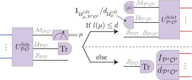
Figure 4: Implementation of the CPTP map Ψ~\widetilde{\Psi} by using the quantum Schur transform [77, 78, 79] and the “measure-and-prepare” strategy [64, 3]. The projective measurement is applied on the Hilbert space 𝒫𝒪\mathcal{M}_{\mathcal{PO}} after the quantum Schur transform. Depending on the measurement outcome μ\mu, we replace a quantum state by a fixed quantum state and apply the inverse of quantum Schur transform to obtain the output state. The wire between 𝒮𝒫𝒪\mathcal{S}_{\mathcal{PO}} and 𝒮𝒫𝒪\mathcal{S}_{\mathcal{P}^{\prime}\mathcal{O}^{\prime}} represents the identity map.

The CPTP map Ψ~\widetilde{\Psi} satisfies the following lemma, which will play a crucial role to construct a parallel isometry inversion protocol.

Lemma 4.

For any isometry operation 𝒱~\widetilde{\mathcal{V}} corresponding to V𝕍iso(d,D)V\in\mathbb{V}_{\mathrm{iso}}(d,D),

Ψ~𝒱~k+1=dU𝒰~k+1\displaystyle\widetilde{\Psi}\circ\widetilde{\mathcal{V}}^{\otimes k+1}=\int{\mathrm{d}}U\widetilde{\mathcal{U}}^{\otimes k+1} (23)

holds, where 𝒰~\widetilde{\mathcal{U}} is a unitary operation corresponding to U𝕌(d)U\in\mathbb{U}(d), and dU{\mathrm{d}}U is the Haar measure on 𝕌(d)\mathbb{U}(d).

This Lemma shows the transformation from k+1k+1 parallel calls of an isometry operation 𝒱~\widetilde{\mathcal{V}} corresponding to V𝕍iso(d,D)V\in\mathbb{V}_{\mathrm{iso}}(d,D) into k+1k+1 parallel calls of a dd-dimensional randomly (and independently of the isometry operator VV) chosen unitary operation. Note that, for D=dD=d, the action of the CPTP map Ψ~\widetilde{\Psi} matches parallel calls of a randomly chosen unitary operation, i.e.,

Ψ~=dU𝒰~k+1.\displaystyle\widetilde{\Psi}=\int{\mathrm{d}}U\widetilde{\mathcal{U}}^{\otimes k+1}. (24)

Then, Lemma 4 reduces to a well-known relation for the Haar measure dU{\mathrm{d}}U on the unitary group 𝕌(d)\mathbb{U}(d) given by

(dU𝒰~k+1)𝒰~k+1=dU𝒰~k+1\displaystyle\left(\int{\mathrm{d}}U\widetilde{\mathcal{U}}^{\otimes k+1}\right)\circ\widetilde{\mathcal{U}}^{\prime\otimes k+1}=\int{\mathrm{d}}U\widetilde{\mathcal{U}}^{\otimes k+1} (25)

for all U𝕌(d)U^{\prime}\in\mathbb{U}(d). In a sense, the CPTP map Ψ~\widetilde{\Psi} extends this relation to an arbitrary DD while keeping the independence on DD on the right hand side, which may be of independent interest. See Appendix H for the proof of Lemma 4.
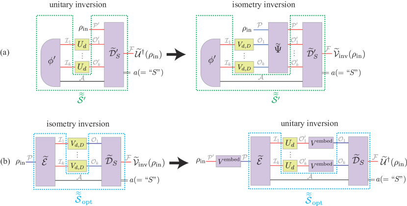
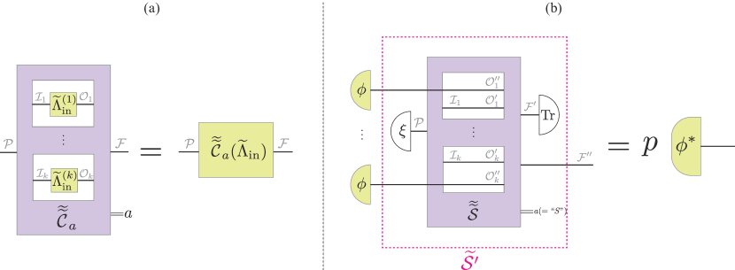
Figure 5: (a) Left panel: Parallel delayed input-state protocol 𝒮~~{\mathchoice{\widetilde{\hbox{$\displaystyle\widetilde{\mathcal{S}^{\prime}}$}}}{\widetilde{\hbox{$\textstyle\widetilde{\mathcal{S}^{\prime}}$}}}{\widetilde{\hbox{$\scriptstyle\widetilde{\mathcal{S}^{\prime}}$}}}{\widetilde{\hbox{$\scriptscriptstyle\widetilde{\mathcal{S}^{\prime}}$}}}} for unitary inversion of Ud𝕌(d)U_{d}\in\mathbb{U}(d) using a quantum state ϕ\phi^{\prime} and a quantum instrument {𝒟~S,𝒟~F}\{\widetilde{\mathcal{D}}^{\prime}_{S},\widetilde{\mathcal{D}}^{\prime}_{F}\} (see also Eq. (10)). Right panel: Construction of a parallel protocol for isometry inversion of Vd,D𝕍iso(d,D)V_{d,D}\in\mathbb{V}_{\mathrm{iso}}(d,D) using a parallel delayed input-state protocol 𝒮~~{\mathchoice{\widetilde{\hbox{$\displaystyle\widetilde{\mathcal{S}^{\prime}}$}}}{\widetilde{\hbox{$\textstyle\widetilde{\mathcal{S}^{\prime}}$}}}{\widetilde{\hbox{$\scriptstyle\widetilde{\mathcal{S}^{\prime}}$}}}{\widetilde{\hbox{$\scriptscriptstyle\widetilde{\mathcal{S}^{\prime}}$}}}} for unitary inversion of Ud𝕌(d)U_{d}\in\mathbb{U}(d) and the CPTP map Ψ~\widetilde{\Psi} defined in Eq. (22). This protocol achieves the same success probability as the parallel delayed-input state protocol for unitary inversion of Ud𝕌(d)U_{d}\in\mathbb{U}(d) shown in the left panel. (b) Left panel: The parallel protocol 𝒮~~opt{\mathchoice{\widetilde{\hbox{$\displaystyle\widetilde{\mathcal{S}}$}}}{\widetilde{\hbox{$\textstyle\widetilde{\mathcal{S}}$}}}{\widetilde{\hbox{$\scriptstyle\widetilde{\mathcal{S}}$}}}{\widetilde{\hbox{$\scriptscriptstyle\widetilde{\mathcal{S}}$}}}}_{\mathrm{opt}} for isometry inversion of Vd,D𝕍iso(d,D)V_{d,D}\in\mathbb{V}_{\mathrm{iso}}(d,D) achieving the optimal success probability can be implemented using a CPTP map ~\widetilde{\mathcal{E}} and a quantum instrument {𝒟~S,𝒟~F}\{\widetilde{\mathcal{D}}_{S},\widetilde{\mathcal{D}}_{F}\} (see also Eq. (36)). Right panel: Construction of a parallel protocol for unitary inversion of Ud𝕌(d)U_{d}\in\mathbb{U}(d) using the optimal parallel protocol 𝒮~~opt{\mathchoice{\widetilde{\hbox{$\displaystyle\widetilde{\mathcal{S}}$}}}{\widetilde{\hbox{$\textstyle\widetilde{\mathcal{S}}$}}}{\widetilde{\hbox{$\scriptstyle\widetilde{\mathcal{S}}$}}}{\widetilde{\hbox{$\scriptscriptstyle\widetilde{\mathcal{S}}$}}}}_{\mathrm{opt}} for isometry inversion of Vd,D𝕍iso(d,D)V_{d,D}\in\mathbb{V}_{\mathrm{iso}}(d,D) and the embedding isometry operator VembedV^{\mathrm{embed}} defined in Eq. (38). This protocol achieves the same success probability as the optimal parallel protocol for isometry inversion shown in the left panel.

Using the CPTP map Ψ~\widetilde{\Psi}, we derive a parallel delayed input-state protocol for isometry inversion protocol as follows. We define a parallel delayed input-state superinstrument {𝒮~~,~~}:[()(𝒪)][(𝒫)()]\{{\mathchoice{\widetilde{\hbox{$\displaystyle\widetilde{\mathcal{S}}$}}}{\widetilde{\hbox{$\textstyle\widetilde{\mathcal{S}}$}}}{\widetilde{\hbox{$\scriptstyle\widetilde{\mathcal{S}}$}}}{\widetilde{\hbox{$\scriptscriptstyle\widetilde{\mathcal{S}}$}}}},{\mathchoice{\widetilde{\hbox{$\displaystyle\widetilde{\mathcal{F}}$}}}{\widetilde{\hbox{$\textstyle\widetilde{\mathcal{F}}$}}}{\widetilde{\hbox{$\scriptstyle\widetilde{\mathcal{F}}$}}}{\widetilde{\hbox{$\scriptscriptstyle\widetilde{\mathcal{F}}$}}}}\}:[\mathcal{L}(\mathcal{I})\to\mathcal{L}(\mathcal{O})]\to[\mathcal{L}(\mathcal{P})\to\mathcal{L}(\mathcal{F})] by inserting the CPTP map Ψ~\widetilde{\Psi} to the parallel delayed input-state superinstrument {𝒮~~,~~}\{{\mathchoice{\widetilde{\hbox{$\displaystyle\widetilde{\mathcal{S}^{\prime}}$}}}{\widetilde{\hbox{$\textstyle\widetilde{\mathcal{S}^{\prime}}$}}}{\widetilde{\hbox{$\scriptstyle\widetilde{\mathcal{S}^{\prime}}$}}}{\widetilde{\hbox{$\scriptscriptstyle\widetilde{\mathcal{S}^{\prime}}$}}}},{\mathchoice{\widetilde{\hbox{$\displaystyle\widetilde{\mathcal{F}^{\prime}}$}}}{\widetilde{\hbox{$\textstyle\widetilde{\mathcal{F}^{\prime}}$}}}{\widetilde{\hbox{$\scriptstyle\widetilde{\mathcal{F}^{\prime}}$}}}{\widetilde{\hbox{$\scriptscriptstyle\widetilde{\mathcal{F}^{\prime}}$}}}}\} for unitary inversion as

𝒮~~(Λ~in)()\displaystyle{\mathchoice{\widetilde{\hbox{$\displaystyle\widetilde{\mathcal{S}}$}}}{\widetilde{\hbox{$\textstyle\widetilde{\mathcal{S}}$}}}{\widetilde{\hbox{$\scriptstyle\widetilde{\mathcal{S}}$}}}{\widetilde{\hbox{$\scriptscriptstyle\widetilde{\mathcal{S}}$}}}}(\widetilde{\Lambda}_{\mathrm{in}})(\cdot) =[𝒟~S(Ψ~𝟙~𝒜)(𝟙~𝒫𝒜Λ~in)](ϕ𝒜),\displaystyle=\left[{\widetilde{\mathcal{D}}^{\prime}_{S}}\circ\left(\widetilde{\Psi}\otimes\widetilde{\mathds{1}}_{\mathcal{A}}\right)\circ\left(\widetilde{\mathds{1}}_{\mathcal{PA}}\otimes\widetilde{\Lambda}_{\mathrm{in}}\right)\right](\cdot\otimes{\phi^{\prime}}_{\mathcal{IA}}), (26)
~~(Λ~in)()\displaystyle{\mathchoice{\widetilde{\hbox{$\displaystyle\widetilde{\mathcal{F}}$}}}{\widetilde{\hbox{$\textstyle\widetilde{\mathcal{F}}$}}}{\widetilde{\hbox{$\scriptstyle\widetilde{\mathcal{F}}$}}}{\widetilde{\hbox{$\scriptscriptstyle\widetilde{\mathcal{F}}$}}}}(\widetilde{\Lambda}_{\mathrm{in}})(\cdot) =[𝒟~F(Ψ~𝟙~𝒜)(𝟙~𝒫𝒜Λ~in)](ϕ𝒜),\displaystyle=\left[{\widetilde{\mathcal{D}}^{\prime}_{F}}\circ\left(\widetilde{\Psi}\otimes\widetilde{\mathds{1}}_{\mathcal{A}}\right)\circ\left(\widetilde{\mathds{1}}_{\mathcal{PA}}\otimes\widetilde{\Lambda}_{\mathrm{in}}\right)\right](\cdot\otimes{\phi^{\prime}}_{\mathcal{IA}}), (27)

where the quantum state ϕ\phi^{\prime} and the quantum instrument {𝒟~S,𝒟~F}\{\widetilde{\mathcal{D}}^{\prime}_{S},\widetilde{\mathcal{D}}^{\prime}_{F}\} are in the superinstrument {𝒮~~,~~}\{{\mathchoice{\widetilde{\hbox{$\displaystyle\widetilde{\mathcal{S}^{\prime}}$}}}{\widetilde{\hbox{$\textstyle\widetilde{\mathcal{S}^{\prime}}$}}}{\widetilde{\hbox{$\scriptstyle\widetilde{\mathcal{S}^{\prime}}$}}}{\widetilde{\hbox{$\scriptscriptstyle\widetilde{\mathcal{S}^{\prime}}$}}}},{\mathchoice{\widetilde{\hbox{$\displaystyle\widetilde{\mathcal{F}^{\prime}}$}}}{\widetilde{\hbox{$\textstyle\widetilde{\mathcal{F}^{\prime}}$}}}{\widetilde{\hbox{$\scriptstyle\widetilde{\mathcal{F}^{\prime}}$}}}{\widetilde{\hbox{$\scriptscriptstyle\widetilde{\mathcal{F}^{\prime}}$}}}}\} for unitary inversion (see Eqs. (10), (11), and Figure 5 (a)). Note that the CPTP map Ψ~\widetilde{\Psi} can be inserted since {𝒮~~,~~}\{{\mathchoice{\widetilde{\hbox{$\displaystyle\widetilde{\mathcal{S}^{\prime}}$}}}{\widetilde{\hbox{$\textstyle\widetilde{\mathcal{S}^{\prime}}$}}}{\widetilde{\hbox{$\scriptstyle\widetilde{\mathcal{S}^{\prime}}$}}}{\widetilde{\hbox{$\scriptscriptstyle\widetilde{\mathcal{S}^{\prime}}$}}}},{\mathchoice{\widetilde{\hbox{$\displaystyle\widetilde{\mathcal{F}^{\prime}}$}}}{\widetilde{\hbox{$\textstyle\widetilde{\mathcal{F}^{\prime}}$}}}{\widetilde{\hbox{$\scriptstyle\widetilde{\mathcal{F}^{\prime}}$}}}{\widetilde{\hbox{$\scriptscriptstyle\widetilde{\mathcal{F}^{\prime}}$}}}}\} is a parallel delayed-input state protocol. If the input state of the parallel delayed-input state protocol 𝒮~~{\mathchoice{\widetilde{\hbox{$\displaystyle\widetilde{\mathcal{S}}$}}}{\widetilde{\hbox{$\textstyle\widetilde{\mathcal{S}}$}}}{\widetilde{\hbox{$\scriptstyle\widetilde{\mathcal{S}}$}}}{\widetilde{\hbox{$\scriptscriptstyle\widetilde{\mathcal{S}}$}}}} is ρin=𝒱~(ρ)\rho_{\mathrm{in}}=\widetilde{\mathcal{V}}(\rho), the output state is calculated as

𝒮~~(𝒱~k)(ρin)\displaystyle{{\mathchoice{\widetilde{\hbox{$\displaystyle\widetilde{\mathcal{S}}$}}}{\widetilde{\hbox{$\textstyle\widetilde{\mathcal{S}}$}}}{\widetilde{\hbox{$\scriptstyle\widetilde{\mathcal{S}}$}}}{\widetilde{\hbox{$\scriptscriptstyle\widetilde{\mathcal{S}}$}}}}(\widetilde{\mathcal{V}}^{\otimes k})(\rho_{\mathrm{in}})} =[𝒮~~(𝒱~k)𝒱~](ρ)\displaystyle={[}{\mathchoice{\widetilde{\hbox{$\displaystyle\widetilde{\mathcal{S}}$}}}{\widetilde{\hbox{$\textstyle\widetilde{\mathcal{S}}$}}}{\widetilde{\hbox{$\scriptstyle\widetilde{\mathcal{S}}$}}}{\widetilde{\hbox{$\scriptscriptstyle\widetilde{\mathcal{S}}$}}}}(\widetilde{\mathcal{V}}^{\otimes k})\circ\widetilde{\mathcal{V}}{]}({\rho}) (28)
=[𝒟~S(Ψ~𝒱~k+1𝟙~𝒜)](ρϕ𝒜)\displaystyle=\left[{\widetilde{\mathcal{D}}^{\prime}_{S}}\circ\left(\widetilde{\Psi}\circ\widetilde{\mathcal{V}}^{\otimes k+1}\otimes\widetilde{\mathds{1}}_{\mathcal{A}}\right)\right]({\rho}\otimes{\phi^{\prime}}_{\mathcal{IA}}) (29)
=dU[𝒟~S(𝒰~k+1𝟙~𝒜)](ρϕ𝒜)\displaystyle=\int{\mathrm{d}}U\left[{\widetilde{\mathcal{D}}^{\prime}_{S}}\circ\left(\widetilde{\mathcal{U}}^{\otimes k+1}\otimes\widetilde{\mathds{1}}_{\mathcal{A}}\right)\right]({\rho}\otimes{\phi^{\prime}}_{\mathcal{IA}}) (30)
=dU[𝒮~~(𝒰~k)𝒰~](ρ)\displaystyle=\int{\mathrm{d}}U\left[{\mathchoice{\widetilde{\hbox{$\displaystyle\widetilde{\mathcal{S}^{\prime}}$}}}{\widetilde{\hbox{$\textstyle\widetilde{\mathcal{S}^{\prime}}$}}}{\widetilde{\hbox{$\scriptstyle\widetilde{\mathcal{S}^{\prime}}$}}}{\widetilde{\hbox{$\scriptscriptstyle\widetilde{\mathcal{S}^{\prime}}$}}}}(\widetilde{\mathcal{U}}^{\otimes k})\circ\widetilde{\mathcal{U}}\right]({\rho}) (31)
=psuccdU(𝒰~𝒰~)(ρ)\displaystyle={p^{\prime}_{\mathrm{succ}}}\int{\mathrm{d}}U\left(\widetilde{\mathcal{U}}^{\dagger}\circ\widetilde{\mathcal{U}}\right)({\rho}) (32)
=psuccρ\displaystyle={p^{\prime}_{\mathrm{succ}}}{\rho} (33)
=psucc𝒱~inv(ρin).\displaystyle={p^{\prime}_{\mathrm{succ}}\widetilde{\mathcal{V}}_{\mathrm{inv}}(\rho_{\mathrm{in}})}. (34)

from Eqs. (12) and (23). Therefore, the quantum superinstrument {𝒮~~,~~}\{{\mathchoice{\widetilde{\hbox{$\displaystyle\widetilde{\mathcal{S}}$}}}{\widetilde{\hbox{$\textstyle\widetilde{\mathcal{S}}$}}}{\widetilde{\hbox{$\scriptstyle\widetilde{\mathcal{S}}$}}}{\widetilde{\hbox{$\scriptscriptstyle\widetilde{\mathcal{S}}$}}}},{\mathchoice{\widetilde{\hbox{$\displaystyle\widetilde{\mathcal{F}}$}}}{\widetilde{\hbox{$\textstyle\widetilde{\mathcal{F}}$}}}{\widetilde{\hbox{$\scriptstyle\widetilde{\mathcal{F}}$}}}{\widetilde{\hbox{$\scriptscriptstyle\widetilde{\mathcal{F}}$}}}}\} implements an isometry inversion protocol and its success probability is psucc{p^{\prime}_{\mathrm{succ}}} when the input quantum state ρin\rho_{\mathrm{in}} is in the image Im𝒱~\mathrm{Im}\widetilde{\mathcal{V}} of the input isometry operation 𝒱~\widetilde{\mathcal{V}}. ∎

3.3 Proof of the main result

Proof of Theorem 1.

We show the first part of Theorem 1, i.e., the optimal success probability of parallel isometry inversion of V𝕍iso(d,D)V\in\mathbb{V}_{\text{iso}}(d,D) coincides with the optimal success probability of parallel unitary inversion of U𝕌(d)U\in\mathbb{U}(d). The achievability is shown by constructing an isometry inversion protocol using Lemma 3. The optimality is shown by constructing a dd-dimensional unitary inversion protocol from a given isometry inversion protocol by embedding 𝕌(d)\mathbb{U}(d) to 𝕍iso(d,D)\mathbb{V}_{\text{iso}}(d,D). The second part of Theorem 1 states the existence of a parallel isometry inversion protocol achieving the success probability psucc=k/(d1)/[d2+k/(d1)1]p_{\mathrm{succ}}=\lfloor k/(d-1)\rfloor/[d^{2}+\lfloor k/(d-1)\rfloor-1] and its optimality for d=2d=2. The existence is shown by constructing an isometry inversion protocol from a corresponding parallel delayed input-state protocol for unitary inversion of U𝕌(d)U\in\mathbb{U}(d) with a success probability psucc=k/(d1)/[d2+k/(d1)1]p_{\mathrm{succ}}=\lfloor k/(d-1)\rfloor/[d^{2}+\lfloor k/(d-1)\rfloor-1] using Lemma 3. Since this parallel unitary inversion protocol is known to be optimal for d=2d=2, this success probability of parallel isometry inversion protocol is optimal for d=2d=2 (see Appendix D and Ref. [18]). We prove the achievability and the optimality of the success probability of isometry inversion as follows.

(Achievability) The optimal success probability popt=popt(d,d,k)p^{\prime}_{\mathrm{opt}}=p_{\mathrm{opt}}(d,d,k) of parallel unitary inversion of U𝕌(d)U\in\mathbb{U}(d) is shown to be achieved by a delayed input-state protocol in Ref. [19]. Using the delayed input-state protocol achieving the optimal success probability poptp^{\prime}_{\mathrm{opt}} with Lemma 3, we show the existence of a parallel protocol for isometry inversion of V𝕍iso(d,D)V\in\mathbb{V}_{\mathrm{iso}}(d,D) with the success probability poptp^{\prime}_{\mathrm{opt}}.

(Optimality) We show the existence of a parallel protocol for unitary inversion of U𝕌(d)U\in\mathbb{U}(d) with the same success probability as the optimal parallel protocol for isometry inversion of V𝕍iso(d,D)V\in\mathbb{V}_{\mathrm{iso}}(d,D) to complete the proof of the first part of Theorem 1. We consider Hilbert spaces 𝒫=D\mathcal{P}=\mathbb{C}^{D}, =d\mathcal{F}=\mathbb{C}^{d}, i=d\mathcal{I}_{i}=\mathbb{C}^{d} and 𝒪i=D\mathcal{O}_{i}=\mathbb{C}^{D} for i{1,,k}i\in\{1,\cdots,k\} and the joint Hilbert spaces \mathcal{I} and 𝒪\mathcal{O} defined as i=1ki\mathcal{I}\coloneqq\bigotimes_{i=1}^{k}\mathcal{I}_{i} and 𝒪i=1k𝒪i\mathcal{O}\coloneqq\bigotimes_{i=1}^{k}\mathcal{O}_{i}, respectively. Suppose {𝒮~~opt,~~opt}:[()(𝒪)][(𝒫)()]\{{\mathchoice{\widetilde{\hbox{$\displaystyle\widetilde{\mathcal{S}}$}}}{\widetilde{\hbox{$\textstyle\widetilde{\mathcal{S}}$}}}{\widetilde{\hbox{$\scriptstyle\widetilde{\mathcal{S}}$}}}{\widetilde{\hbox{$\scriptscriptstyle\widetilde{\mathcal{S}}$}}}}_{\mathrm{opt}},{\mathchoice{\widetilde{\hbox{$\displaystyle\widetilde{\mathcal{F}}$}}}{\widetilde{\hbox{$\textstyle\widetilde{\mathcal{F}}$}}}{\widetilde{\hbox{$\scriptstyle\widetilde{\mathcal{F}}$}}}{\widetilde{\hbox{$\scriptscriptstyle\widetilde{\mathcal{F}}$}}}}_{\mathrm{opt}}\}:[\mathcal{L}(\mathcal{I})\to\mathcal{L}(\mathcal{O})]\to[\mathcal{L}(\mathcal{P})\to\mathcal{L}(\mathcal{F})] be a kk-input parallel superinstrument implementing isometry inversion of V𝕍iso(d,D)V\in\mathbb{V}_{\mathrm{iso}}(d,D) with the optimal success probability popt=popt(d,D,k)p_{\mathrm{opt}}=p_{\mathrm{opt}}(d,D,k), i.e.,

𝒮~~opt(𝒱~k)(ρin)=popt𝒱~inv(ρin)(V𝕍iso(d,D),ρin(ImV)).\displaystyle{\mathchoice{\widetilde{\hbox{$\displaystyle\widetilde{\mathcal{S}}$}}}{\widetilde{\hbox{$\textstyle\widetilde{\mathcal{S}}$}}}{\widetilde{\hbox{$\scriptstyle\widetilde{\mathcal{S}}$}}}{\widetilde{\hbox{$\scriptscriptstyle\widetilde{\mathcal{S}}$}}}}_{\mathrm{opt}}(\widetilde{\mathcal{V}}^{\otimes k})(\rho_{\mathrm{in}})=p_{\mathrm{opt}}\widetilde{\mathcal{V}}_{\mathrm{inv}}(\rho_{\mathrm{in}})\;\;\;(\forall V\in\mathbb{V}_{\mathrm{iso}}(d,D),\forall\rho_{\mathrm{in}}\in\mathcal{L}(\mathrm{Im}V)). (35)

The parallel superinstrument {𝒮~~opt,~~opt}\{{\mathchoice{\widetilde{\hbox{$\displaystyle\widetilde{\mathcal{S}}$}}}{\widetilde{\hbox{$\textstyle\widetilde{\mathcal{S}}$}}}{\widetilde{\hbox{$\scriptstyle\widetilde{\mathcal{S}}$}}}{\widetilde{\hbox{$\scriptscriptstyle\widetilde{\mathcal{S}}$}}}}_{\mathrm{opt}},{\mathchoice{\widetilde{\hbox{$\displaystyle\widetilde{\mathcal{F}}$}}}{\widetilde{\hbox{$\textstyle\widetilde{\mathcal{F}}$}}}{\widetilde{\hbox{$\scriptstyle\widetilde{\mathcal{F}}$}}}{\widetilde{\hbox{$\scriptscriptstyle\widetilde{\mathcal{F}}$}}}}_{\mathrm{opt}}\} can be written as

𝒮~~opt(Λ~in)\displaystyle{\mathchoice{\widetilde{\hbox{$\displaystyle\widetilde{\mathcal{S}}$}}}{\widetilde{\hbox{$\textstyle\widetilde{\mathcal{S}}$}}}{\widetilde{\hbox{$\scriptstyle\widetilde{\mathcal{S}}$}}}{\widetilde{\hbox{$\scriptscriptstyle\widetilde{\mathcal{S}}$}}}}_{\mathrm{opt}}(\widetilde{\Lambda}_{\mathrm{in}}) =𝒟~S(Λ~in𝟙~𝒜)~,\displaystyle=\widetilde{\mathcal{D}}_{S}\circ\left(\widetilde{\Lambda}_{\mathrm{in}}\otimes\widetilde{\mathds{1}}_{\mathcal{A}}\right)\circ\widetilde{\mathcal{E}}, (36)
~~opt(Λ~in)\displaystyle{\mathchoice{\widetilde{\hbox{$\displaystyle\widetilde{\mathcal{F}}$}}}{\widetilde{\hbox{$\textstyle\widetilde{\mathcal{F}}$}}}{\widetilde{\hbox{$\scriptstyle\widetilde{\mathcal{F}}$}}}{\widetilde{\hbox{$\scriptscriptstyle\widetilde{\mathcal{F}}$}}}}_{\mathrm{opt}}(\widetilde{\Lambda}_{\mathrm{in}}) =𝒟~F(Λ~in𝟙~𝒜)~,\displaystyle=\widetilde{\mathcal{D}}_{F}\circ\left(\widetilde{\Lambda}_{\mathrm{in}}\otimes\widetilde{\mathds{1}}_{\mathcal{A}}\right)\circ\widetilde{\mathcal{E}}, (37)

where 𝒜\mathcal{A} is an auxiliary Hilbert space, ~:(𝒫)(𝒜)\widetilde{\mathcal{E}}:\mathcal{L}(\mathcal{P})\to\mathcal{L}(\mathcal{I}\otimes\mathcal{A}) is a CPTP map, and {𝒟~S,𝒟~F}\{\widetilde{\mathcal{D}}_{S},\widetilde{\mathcal{D}}_{F}\} is a quantum instrument (see the left panel of Figure 5 (b)).

We construct a parallel protocol for unitary inversion of U𝕌(d)U\in\mathbb{U}(d) with the same success probability poptp_{\mathrm{opt}} as the parallel protocol for isometry inversion of Vd,D𝕍iso(d,D)V_{d,D}\in\mathbb{V}_{\mathrm{iso}}(d,D) as follows. We consider Hilbert spaces 𝒫=d\mathcal{P}^{\prime}=\mathbb{C}^{d} and 𝒪i=d\mathcal{O}^{\prime}_{i}=\mathbb{C}^{d} for i{1,,k}i\in\{1,\cdots,k\} and the joint Hilbert space 𝒪i=1k𝒪i\mathcal{O}^{\prime}\coloneqq\bigotimes_{i=1}^{k}\mathcal{O}^{\prime}_{i}. We define the embedding isometry operator Vembed:dDV^{\mathrm{embed}}:\mathbb{C}^{d}\to\mathbb{C}^{D} as

Vembedi=0d1|iDi|d,\displaystyle V^{\mathrm{embed}}\coloneqq\sum_{i=0}^{d-1}|{i}\rangle_{\mathbb{C}^{D}}\langle{i}|_{\mathbb{C}^{d}}, (38)

where {|i}i=0d1\{|{i}\rangle\}_{i=0}^{d-1} and {|i}i=0D1\{|{i}\rangle\}_{i=0}^{D-1} are the computational bases of d\mathbb{C}^{d} and D\mathbb{C}^{D}, respectively. By defining {𝒮~~,~~}:[()(𝒪)][(𝒫)()]\{{\mathchoice{\widetilde{\hbox{$\displaystyle\widetilde{\mathcal{S}^{\prime}}$}}}{\widetilde{\hbox{$\textstyle\widetilde{\mathcal{S}^{\prime}}$}}}{\widetilde{\hbox{$\scriptstyle\widetilde{\mathcal{S}^{\prime}}$}}}{\widetilde{\hbox{$\scriptscriptstyle\widetilde{\mathcal{S}^{\prime}}$}}}},{\mathchoice{\widetilde{\hbox{$\displaystyle\widetilde{\mathcal{F}^{\prime}}$}}}{\widetilde{\hbox{$\textstyle\widetilde{\mathcal{F}^{\prime}}$}}}{\widetilde{\hbox{$\scriptstyle\widetilde{\mathcal{F}^{\prime}}$}}}{\widetilde{\hbox{$\scriptscriptstyle\widetilde{\mathcal{F}^{\prime}}$}}}}\}:[\mathcal{L}(\mathcal{I})\to\mathcal{L}(\mathcal{O}^{\prime})]\to[\mathcal{L}(\mathcal{P}^{\prime})\to\mathcal{L}(\mathcal{F})] as

𝒮~~(Λ~in)\displaystyle{\mathchoice{\widetilde{\hbox{$\displaystyle\widetilde{\mathcal{S}^{\prime}}$}}}{\widetilde{\hbox{$\textstyle\widetilde{\mathcal{S}^{\prime}}$}}}{\widetilde{\hbox{$\scriptstyle\widetilde{\mathcal{S}^{\prime}}$}}}{\widetilde{\hbox{$\scriptscriptstyle\widetilde{\mathcal{S}^{\prime}}$}}}}(\widetilde{\Lambda}_{\mathrm{in}})\coloneqq 𝒟~S[(i=1k𝒱~𝒪i𝒪iembedΛ~in)𝟙~𝒜]~𝒱~𝒫𝒫embed,\displaystyle\widetilde{\mathcal{D}}_{S}\circ\left[\left(\bigotimes_{i=1}^{k}\widetilde{\mathcal{V}}^{\mathrm{embed}}_{\mathcal{O}^{\prime}_{i}\to\mathcal{O}_{i}}\circ\widetilde{\Lambda}_{\mathrm{in}}\right)\otimes\widetilde{\mathds{1}}_{\mathcal{A}}\right]\circ\widetilde{\mathcal{E}}\circ\widetilde{\mathcal{V}}^{\mathrm{embed}}_{\mathcal{P}^{\prime}\to\mathcal{P}}, (39)
~~(Λ~in)\displaystyle{\mathchoice{\widetilde{\hbox{$\displaystyle\widetilde{\mathcal{F}^{\prime}}$}}}{\widetilde{\hbox{$\textstyle\widetilde{\mathcal{F}^{\prime}}$}}}{\widetilde{\hbox{$\scriptstyle\widetilde{\mathcal{F}^{\prime}}$}}}{\widetilde{\hbox{$\scriptscriptstyle\widetilde{\mathcal{F}^{\prime}}$}}}}(\widetilde{\Lambda}_{\mathrm{in}})\coloneqq 𝒟~F[(i=1k𝒱~𝒪i𝒪iembedΛ~in)𝟙~𝒜]~𝒱~𝒫𝒫embed,\displaystyle\widetilde{\mathcal{D}}_{F}\circ\left[\left(\bigotimes_{i=1}^{k}\widetilde{\mathcal{V}}^{\mathrm{embed}}_{\mathcal{O}^{\prime}_{i}\to\mathcal{O}_{i}}\circ\widetilde{\Lambda}_{\mathrm{in}}\right)\otimes\widetilde{\mathds{1}}_{\mathcal{A}}\right]\circ\widetilde{\mathcal{E}}\circ\widetilde{\mathcal{V}}^{\mathrm{embed}}_{\mathcal{P}^{\prime}\to\mathcal{P}}, (40)

{𝒮~~,~~}\{{\mathchoice{\widetilde{\hbox{$\displaystyle\widetilde{\mathcal{S}^{\prime}}$}}}{\widetilde{\hbox{$\textstyle\widetilde{\mathcal{S}^{\prime}}$}}}{\widetilde{\hbox{$\scriptstyle\widetilde{\mathcal{S}^{\prime}}$}}}{\widetilde{\hbox{$\scriptscriptstyle\widetilde{\mathcal{S}^{\prime}}$}}}},{\mathchoice{\widetilde{\hbox{$\displaystyle\widetilde{\mathcal{F}^{\prime}}$}}}{\widetilde{\hbox{$\textstyle\widetilde{\mathcal{F}^{\prime}}$}}}{\widetilde{\hbox{$\scriptstyle\widetilde{\mathcal{F}^{\prime}}$}}}{\widetilde{\hbox{$\scriptscriptstyle\widetilde{\mathcal{F}^{\prime}}$}}}}\} is a parallel superinstrument as shown in Figure 5 (b). Since VembedUV^{\mathrm{embed}}U is an isometry operator for all U𝕌(d)U\in\mathbb{U}(d), we obtain

𝒮~~(𝒰~k)=popt(𝒱~embed𝒰~)inv𝒱~embed\displaystyle{\mathchoice{\widetilde{\hbox{$\displaystyle\widetilde{\mathcal{S}^{\prime}}$}}}{\widetilde{\hbox{$\textstyle\widetilde{\mathcal{S}^{\prime}}$}}}{\widetilde{\hbox{$\scriptstyle\widetilde{\mathcal{S}^{\prime}}$}}}{\widetilde{\hbox{$\scriptscriptstyle\widetilde{\mathcal{S}^{\prime}}$}}}}(\widetilde{\mathcal{U}}^{\otimes k})=p_{\mathrm{opt}}(\widetilde{\mathcal{V}}^{\mathrm{embed}}\circ\widetilde{\mathcal{U}})_{\mathrm{inv}}\circ\widetilde{\mathcal{V}}^{\mathrm{embed}} (41)

for all U𝕌(d)U\in\mathbb{U}(d) from Eq. (35). Since the inverse operation of an isometry operation is defined as Eq. (2),

𝒮~~(𝒰~k)𝒰~\displaystyle{\mathchoice{\widetilde{\hbox{$\displaystyle\widetilde{\mathcal{S}^{\prime}}$}}}{\widetilde{\hbox{$\textstyle\widetilde{\mathcal{S}^{\prime}}$}}}{\widetilde{\hbox{$\scriptstyle\widetilde{\mathcal{S}^{\prime}}$}}}{\widetilde{\hbox{$\scriptscriptstyle\widetilde{\mathcal{S}^{\prime}}$}}}}(\widetilde{\mathcal{U}}^{\otimes k})\circ\widetilde{\mathcal{U}} =popt(𝒱~embed𝒰~)inv𝒱~embed𝒰~\displaystyle=p_{\mathrm{opt}}(\widetilde{\mathcal{V}}^{\mathrm{embed}}\circ\widetilde{\mathcal{U}})_{\mathrm{inv}}\circ\widetilde{\mathcal{V}}^{\mathrm{embed}}\circ\widetilde{\mathcal{U}} (42)
=popt𝟙~d,\displaystyle=p_{\mathrm{opt}}\widetilde{\mathds{1}}_{d}, (43)

i.e.,

𝒮~~(𝒰~k)=popt𝒰~\displaystyle{\mathchoice{\widetilde{\hbox{$\displaystyle\widetilde{\mathcal{S}^{\prime}}$}}}{\widetilde{\hbox{$\textstyle\widetilde{\mathcal{S}^{\prime}}$}}}{\widetilde{\hbox{$\scriptstyle\widetilde{\mathcal{S}^{\prime}}$}}}{\widetilde{\hbox{$\scriptscriptstyle\widetilde{\mathcal{S}^{\prime}}$}}}}(\widetilde{\mathcal{U}}^{\otimes k})=p_{\mathrm{opt}}\widetilde{\mathcal{U}}^{\dagger} (44)

holds for all U𝕌(d)U\in\mathbb{U}(d). Therefore, the parallel superinstrument {𝒮~~,~~}\{{\mathchoice{\widetilde{\hbox{$\displaystyle\widetilde{\mathcal{S}^{\prime}}$}}}{\widetilde{\hbox{$\textstyle\widetilde{\mathcal{S}^{\prime}}$}}}{\widetilde{\hbox{$\scriptstyle\widetilde{\mathcal{S}^{\prime}}$}}}{\widetilde{\hbox{$\scriptscriptstyle\widetilde{\mathcal{S}^{\prime}}$}}}},{\mathchoice{\widetilde{\hbox{$\displaystyle\widetilde{\mathcal{F}^{\prime}}$}}}{\widetilde{\hbox{$\textstyle\widetilde{\mathcal{F}^{\prime}}$}}}{\widetilde{\hbox{$\scriptstyle\widetilde{\mathcal{F}^{\prime}}$}}}{\widetilde{\hbox{$\scriptscriptstyle\widetilde{\mathcal{F}^{\prime}}$}}}}\} implements unitary inversion of U𝕌(d)U\in\mathbb{U}(d) with the success probability poptp_{\mathrm{opt}}. This completes the proof of the first part of Theorem 1. As stated in the first paragraph of the proof, the second part (achievability of the success probability psucc=k/(d1)/[d2+k/(d1)1]p_{\mathrm{succ}}=\lfloor k/(d-1)\rfloor/[d^{2}+\lfloor k/(d-1)\rfloor-1]) of Theorem 1 follows from the combination of the first part and a parallel delayed input-state protocol for unitary inversion shown in Appendix D and Ref. [18]. ∎

Figure 6: (a) Unitary embedding strategy for isometry inversion. By inverting a unitary operation UVU_{V} satisfying V|ψ=UV(|ψ|aux)V|{\psi}\rangle=U_{V}(|{\psi}\rangle\otimes|{\mathrm{aux}}\rangle), we obtain the inverse map of an isometry operation 𝒱~\widetilde{\mathcal{V}}. (b) Comparison of the success probability of the two protocols for isometry inversion using kk calls of V𝕍iso(2,25)V\in\mathbb{V}_{\mathrm{iso}}(2,2^{5}) or UV𝕌(25)U_{V}\in\mathbb{U}(2^{5}): the parallel protocol shown in Figure 2 (a) (blue line) and the strategy based on the embedding of the input isometry operation VV in a unitary operation UVU_{V} (red dotted line).

3.4 Analysis of other related settings

3.4.1 Unitary embedding strategy

for D=ddD=dd^{\prime}, any isometry operator V𝕍iso(d,D)V\in\mathbb{V}_{\mathrm{iso}}(d,D) can be embedded in an appropriate unitary operation UV𝕌(D)U_{V}\in\mathbb{U}(D) by adding a fixed auxiliary system |auxd|{\mathrm{aux}}\rangle\in\mathbb{C}^{d^{\prime}} and seeking UVU_{V} satisfying

V|ψ=UV(|ψ|aux)\displaystyle V|{\psi}\rangle=U_{V}(|{\psi}\rangle\otimes|{\mathrm{aux}}\rangle) (45)

for all |ψd|{\psi}\rangle\in\mathbb{C}^{d} (see Figure 6 (a)). Assuming that the black box implementing UVU_{V} and the fixed auxiliary state are given, we can implement an inverse map of 𝒱~\widetilde{\mathcal{V}} by applying the unitary inversion protocol. Any DD-dimensional unitary inversion protocol needs at least D1D-1 calls of an input unitary operation to be successful with a non-zero probability [18]. In contrast, our direct isometry inversion protocol using kk parallel calls of an input isometry operation 𝒱~\widetilde{\mathcal{V}} corresponding to V𝕍iso(d,D)V\in\mathbb{V}_{\mathrm{iso}}(d,D) implements the inverse map 𝒱~inv\widetilde{\mathcal{V}}_{\mathrm{inv}} with a success probability psucc=k/(d1)/[d2+k/(d1)1]p_{\mathrm{succ}}=\lfloor k/(d-1)\rfloor/[d^{2}+\lfloor k/(d-1)\rfloor-1]. We compare these success probabilities for d=2,D=25d=2,D=2^{5} and 1k201\leq k\leq 20 (see Figure 6 (b)). The isometry inversion protocol achieves a success probability psucc87%p_{\mathrm{succ}}\approx 87\% at k=20k=20, while probabilistic unitary inversion is impossible for any k30k\leq 30.

3.4.2 Process tomography strategy

Approximate isometry inversion can be achieved by approximating the classical description of V𝕍iso(d,D)V\in\mathbb{V}_{\mathrm{iso}}(d,D) by quantum process tomography first [1, 65], and then applying the inverse map calculated from the classical description. Quantum process tomography consists of three steps: preparing a quantum state called a probe state, applying a black box quantum operation to a probe state, and performing a measurement on the output state. By repeating this procedure, we obtain a probability distribution of measurement outcomes to estimate a black box operation. An isometry operator V𝕍iso(d,D)V\in\mathbb{V}_{\mathrm{iso}}(d,D) is uniquely specified by 2Ddd2+d1=Ω(Dd)2Dd-d^{2}+d-1=\Omega(Dd) real parameters55 5 We say f(x)=Ω(g(x))f(x)=\Omega(g(x)) if lim supx|f(x)/g(x)|>0\limsup_{x\to\infty}{|f(x)/g(x)|}>0., and Ω(ϵ2ln(1/(1p)))\Omega(\epsilon^{-2}\ln(1/(1-p))) measurements are necessary to estimate each parameter with at most error ϵ\epsilon and at least probability pp [65]. Therefore, we need Ω(Ddϵ2ln(1/(1p)))\Omega(Dd\epsilon^{-2}\ln(1/(1-p))) calls of an isometry operation 𝒱~\widetilde{\mathcal{V}} for the process tomography of VV. On the other hand, since we can achieve the success probability psucc=k/(d1)/[d2+k/(d1)1]p_{\mathrm{succ}}=\lfloor k/(d-1)\rfloor/[d^{2}+\lfloor k/(d-1)\rfloor-1] by kk parallel calls of an isometry operation 𝒱~\widetilde{\mathcal{V}}, the success probability becomes psuccp_{\text{succ}} for k=(d1)(d21)/(1psucc)=𝒪(d3/(1psucc))k=(d-1)(d^{2}-1)/(1-p_{\text{succ}})=\mathcal{O}(d^{3}/(1-p_{\text{succ}})).66 6 We say f(x)=𝒪(g(x))f(x)=\mathcal{O}(g(x)) if lim supx|f(x)/g(x)|<\limsup_{x\to\infty}{|f(x)/g(x)|}<\infty. The isometry inversion protocol outperforms the strategy based on process tomography at two points. First, the isometry inversion protocol can implement the inverse operation without error (ϵ=0\epsilon=0) using finite calls of 𝒱~\widetilde{\mathcal{V}}, while the process tomography needs Ω(ϵ2)\Omega(\epsilon^{-2}) calls to achieve the error below ϵ\epsilon. Second, the isometry inversion protocol can be done with a DD-independent number of calls of 𝒱~\widetilde{\mathcal{V}}, while the process tomography requires a DD-dependent number of calls. Though the scaling of the number of calls in our protocol with respect to psuccp_{\mathrm{succ}} is polynomial, we also find a protocol with k=𝒪(ln(1/(1psucc)))k=\mathcal{O}(\ln(1/(1-p_{\mathrm{succ}}))) using a “success-or-draw” protocol for d=2d=2 and D=3D=3, whose existence is shown numerically (see Section 5).

4 Difference between isometry inversion protocols and unitary inversion protocols

The parallel unitary inversion protocol presented in Ref. [18] consists of a concatenation of unitary complex conjugation and unitary transposition. The implementation of unitary complex conjugation shown in Ref. [15] relies on the fact that the complex conjugate representation of 𝕌(d)\mathbb{U}(d) is unitarily equivalent to the antisymmetric subspace in the tensor representation of 𝕌(d)\mathbb{U}(d) on (d)d1(\mathbb{C}^{d})^{\otimes d-1}. The unitary transposition protocol presented in Ref. [19] utilizes a variant of gate teleportation [66] or the probabilistic port-based teleportation [67, 68]. In contrast, we show that isometry inversion protocols cannot be decomposed into isometry complex conjugation and isometry transposition. We can consider another similar strategy by considering “isometry pseudo complex conjugation”, but this strategy is shown to be inefficient. We first investigate protocols for isometry complex conjugation and isometry pseudo complex conjugation, and then analyze the difference between isometry inversion and unitary inversion in this section. Isometry transposition is investigated in Appendix E.

4.1 The no-go theorem for isometry complex conjugation

We prove that any isometry inversion protocol cannot be decomposed into isometry complex conjugation and isometry transposition by showing a no-go theorem for isometry complex conjugation.

To state the no-go theorem properly, we introduce the notion of general superinstrument including the ones with an indefinite causal order [70, 71, 72, 73, 74, 75, 76], which describes the most general higher-order probabilistic transformation where the order of the use of the input maps is not pre-determined. Using the same notations of the Hilbert spaces and the input maps introduced for a superinstrument in Section 2.2, a general superinstrument is a set of kk-input supermaps {𝒞~~a}:[()(𝒪)][(𝒫)()]\{{\mathchoice{\widetilde{\hbox{$\displaystyle\widetilde{\mathcal{C}}$}}}{\widetilde{\hbox{$\textstyle\widetilde{\mathcal{C}}$}}}{\widetilde{\hbox{$\scriptstyle\widetilde{\mathcal{C}}$}}}{\widetilde{\hbox{$\scriptscriptstyle\widetilde{\mathcal{C}}$}}}}_{a}\}:[\mathcal{L}(\mathcal{I})\to\mathcal{L}(\mathcal{O})]\to[\mathcal{L}(\mathcal{P})\to\mathcal{L}(\mathcal{F})] such that a set of output maps {𝒞~~a𝟙~~(Λ~in)}a\{{\mathchoice{\widetilde{\hbox{$\displaystyle\widetilde{\mathcal{C}}$}}}{\widetilde{\hbox{$\textstyle\widetilde{\mathcal{C}}$}}}{\widetilde{\hbox{$\scriptstyle\widetilde{\mathcal{C}}$}}}{\widetilde{\hbox{$\scriptscriptstyle\widetilde{\mathcal{C}}$}}}}_{a}\otimes{\mathchoice{\widetilde{\hbox{$\displaystyle\widetilde{\mathds{1}}$}}}{\widetilde{\hbox{$\textstyle\widetilde{\mathds{1}}$}}}{\widetilde{\hbox{$\scriptstyle\widetilde{\mathds{1}}$}}}{\widetilde{\hbox{$\scriptscriptstyle\widetilde{\mathds{1}}$}}}}(\widetilde{\Lambda}_{\mathrm{in}})\}_{a} is a quantum instrument for any set of input CPTP maps {Λ~in(i)}i=1k\{\widetilde{\Lambda}_{\mathrm{in}}^{(i)}\}_{i=1}^{k}, where 𝟙~~{\mathchoice{\widetilde{\hbox{$\displaystyle\widetilde{\mathds{1}}$}}}{\widetilde{\hbox{$\textstyle\widetilde{\mathds{1}}$}}}{\widetilde{\hbox{$\scriptstyle\widetilde{\mathds{1}}$}}}{\widetilde{\hbox{$\scriptscriptstyle\widetilde{\mathds{1}}$}}}} is the identity supermap defined by 𝟙~~(Λ~)=Λ~{\mathchoice{\widetilde{\hbox{$\displaystyle\widetilde{\mathds{1}}$}}}{\widetilde{\hbox{$\textstyle\widetilde{\mathds{1}}$}}}{\widetilde{\hbox{$\scriptstyle\widetilde{\mathds{1}}$}}}{\widetilde{\hbox{$\scriptscriptstyle\widetilde{\mathds{1}}$}}}}(\widetilde{\Lambda})=\widetilde{\Lambda}. This definition of a general superinstrument {𝒞~~a}\{{\mathchoice{\widetilde{\hbox{$\displaystyle\widetilde{\mathcal{C}}$}}}{\widetilde{\hbox{$\textstyle\widetilde{\mathcal{C}}$}}}{\widetilde{\hbox{$\scriptstyle\widetilde{\mathcal{C}}$}}}{\widetilde{\hbox{$\scriptscriptstyle\widetilde{\mathcal{C}}$}}}}_{a}\} states that a set of output maps is a quantum instrument even if the superinstrument acts on a subsystem of input CPTP maps. Note that the condition that 𝒞~~a𝟙~~(Λ~in){\mathchoice{\widetilde{\hbox{$\displaystyle\widetilde{\mathcal{C}}$}}}{\widetilde{\hbox{$\textstyle\widetilde{\mathcal{C}}$}}}{\widetilde{\hbox{$\scriptstyle\widetilde{\mathcal{C}}$}}}{\widetilde{\hbox{$\scriptscriptstyle\widetilde{\mathcal{C}}$}}}}_{a}\otimes{\mathchoice{\widetilde{\hbox{$\displaystyle\widetilde{\mathds{1}}$}}}{\widetilde{\hbox{$\textstyle\widetilde{\mathds{1}}$}}}{\widetilde{\hbox{$\scriptstyle\widetilde{\mathds{1}}$}}}{\widetilde{\hbox{$\scriptscriptstyle\widetilde{\mathds{1}}$}}}}(\widetilde{\Lambda}_{\mathrm{in}}) is a quantum instrument for any input CPTP maps {Λ~in(i)}i=1k\{\widetilde{\Lambda}_{\mathrm{in}}^{(i)}\}_{i=1}^{k}, is strictly stronger than the relaxed condition that (b) 𝒞~~a(Λ~in){\mathchoice{\widetilde{\hbox{$\displaystyle\widetilde{\mathcal{C}}$}}}{\widetilde{\hbox{$\textstyle\widetilde{\mathcal{C}}$}}}{\widetilde{\hbox{$\scriptstyle\widetilde{\mathcal{C}}$}}}{\widetilde{\hbox{$\scriptscriptstyle\widetilde{\mathcal{C}}$}}}}_{a}(\widetilde{\Lambda}_{\mathrm{in}}) is a quantum instrument for any input CPTP maps {Λ~in(i)}i=1k\{\widetilde{\Lambda}_{\mathrm{in}}^{(i)}\}_{i=1}^{k}, which is similar to the distinction between positive maps and completely positive maps.

A general superinstrument {𝒞~~a}\{{\mathchoice{\widetilde{\hbox{$\displaystyle\widetilde{\mathcal{C}}$}}}{\widetilde{\hbox{$\textstyle\widetilde{\mathcal{C}}$}}}{\widetilde{\hbox{$\scriptstyle\widetilde{\mathcal{C}}$}}}{\widetilde{\hbox{$\scriptscriptstyle\widetilde{\mathcal{C}}$}}}}_{a}\} is not necessarily represented by a quantum circuit, which requires to fix a causal ordering of the use of the input maps. To illustrate a protocol using a general supermap in a similar manner of quantum circuits, we use a notation of a general supermap represented by a box with windows for plugging input maps (see Figure 7 (a)). As the windows of the box are not causally ordered, the box represents a general supermap, a transformation of input maps with unspecified order to the output map77 7 This notation is adopted from Ref. [75]..

Using the notion of general superinstrument, we can state the following no-go theorem for isometry complex conjugation.

Theorem 5.

If D2dD\geq 2d, it is impossible to transform finite calls of an isometry operation 𝒱~:(d)(D)\widetilde{\mathcal{V}}:\mathcal{L}(\mathbb{C}^{d})\to\mathcal{L}(\mathbb{C}^{D}) into its complex conjugate map 𝒱~\widetilde{\mathcal{V}}^{*} with a non-zero success probability using any general superinstrument.

Note that this no-go theorem states the impossibility of isometry complex conjugation from finite calls even if we can implement a general superinstrument, which is beyond the quantum circuit model. To prove this no-go theorem, we first show the impossibility for DD is a multiple of dd.

Figure 7: (a) The left hand side shows an illustration of a general superinstrument {𝒞~~a}\{{\mathchoice{\widetilde{\hbox{$\displaystyle\widetilde{\mathcal{C}}$}}}{\widetilde{\hbox{$\textstyle\widetilde{\mathcal{C}}$}}}{\widetilde{\hbox{$\scriptstyle\widetilde{\mathcal{C}}$}}}{\widetilde{\hbox{$\scriptscriptstyle\widetilde{\mathcal{C}}$}}}}_{a}\} as a purple box with windows where input maps Λ~in(i)(i{1,,k})\widetilde{\Lambda}_{\mathrm{in}}^{(i)}\;(i\in\{1,\cdots,k\}) are plugged. The right hand side is the output map of a general superinstrument {𝒞~~a}\{{\mathchoice{\widetilde{\hbox{$\displaystyle\widetilde{\mathcal{C}}$}}}{\widetilde{\hbox{$\textstyle\widetilde{\mathcal{C}}$}}}{\widetilde{\hbox{$\scriptstyle\widetilde{\mathcal{C}}$}}}{\widetilde{\hbox{$\scriptscriptstyle\widetilde{\mathcal{C}}$}}}}_{a}\} for input maps Λ~in(i)\widetilde{\Lambda}_{\mathrm{in}}^{(i)}. (b) A hypothetical protocol using a general superinstrument {𝒮~~,~~}\{{\mathchoice{\widetilde{\hbox{$\displaystyle\widetilde{\mathcal{S}}$}}}{\widetilde{\hbox{$\textstyle\widetilde{\mathcal{S}}$}}}{\widetilde{\hbox{$\scriptstyle\widetilde{\mathcal{S}}$}}}{\widetilde{\hbox{$\scriptscriptstyle\widetilde{\mathcal{S}}$}}}},{\mathchoice{\widetilde{\hbox{$\displaystyle\widetilde{\mathcal{F}}$}}}{\widetilde{\hbox{$\textstyle\widetilde{\mathcal{F}}$}}}{\widetilde{\hbox{$\scriptstyle\widetilde{\mathcal{F}}$}}}{\widetilde{\hbox{$\scriptscriptstyle\widetilde{\mathcal{F}}$}}}}\} for isometry complex conjugation to prove Lemma 6 by contradiction. The wire between i\mathcal{I}_{i} and 𝒪i\mathcal{O}_{i} (i{1,,k}i\in\{1,\cdots,k\}) represent the identity map and ξ\xi is an arbitrary quantum state.
Lemma 6.

Let dd^{\prime} be a natural number greater than 1. If D=ddD=dd^{\prime}, it is impossible to transform finite calls of an isometry operation 𝒱~:(d)(D)\widetilde{\mathcal{V}}:\mathcal{L}(\mathbb{C}^{d})\to\mathcal{L}(\mathbb{C}^{D}) into its complex conjugate map 𝒱~\widetilde{\mathcal{V}}^{*} with a non-zero success probability using any general superinstrument.

Proof.

We prove this Lemma by contradiction. Probabilistic exact state complex conjugation of |ϕ|{\phi}\rangle is shown to be possible by applying probabilistic isometry complex conjugation to an isometry operator V|ϕV_{|{\phi}\rangle}, which joints an auxiliary quantum state |ϕ|{\phi}\rangle to an input state. If probabilistic isometry complex conjugation can be implemented with a non-zero success probability, probabilistic exact state complex conjugation is also possible with a non-zero success probability, which contradicts the no-go theorem of state complex conjugation88 8 The impossibility of probabilistic exact state complex conjugation |ϕk|ϕ|{\phi}\rangle^{\otimes k}\mapsto|{\phi^{*}}\rangle can be easily understood for k=1k=1. Since |ϕϕ|=|ϕϕ|T|{\phi^{*}}\rangle\!\langle{\phi^{*}}|=|{\phi}\rangle\!\langle{\phi}|^{T} holds due to the hermicity of |ϕϕ||{\phi}\rangle\!\langle{\phi}|, a quantum instrument {𝒮~,~}\{\widetilde{\mathcal{S}}^{\prime},\widetilde{\mathcal{F}}^{\prime}\} satisfies 𝒮~(|ϕϕ|)=psucc|ϕϕ|\widetilde{\mathcal{S}}^{\prime}(|{\phi}\rangle\!\langle{\phi}|)=p_{\text{succ}}|{\phi^{*}}\rangle\!\langle{\phi^{*}}| if and only if 𝒮~(ρ)=psuccρT\widetilde{\mathcal{S}}^{\prime}(\rho)=p_{\text{succ}}\rho^{T} for any ρ()\rho\in\mathcal{L}(\mathcal{H}). However, since transposition of a state is not completely positive, any quantum instrument {𝒮~,~}\{\widetilde{\mathcal{S}}^{\prime},\widetilde{\mathcal{F}}^{\prime}\} does not achieve non-zero success probability. [80]. See Figure 7 (b) for a hypothetical protocol using a general superinstrument to prove this Lemma by contradiction.

We consider a kk-input general superinstrument {𝒮~~,~~}:[()(𝒪)][(𝒫)()]\{{\mathchoice{\widetilde{\hbox{$\displaystyle\widetilde{\mathcal{S}}$}}}{\widetilde{\hbox{$\textstyle\widetilde{\mathcal{S}}$}}}{\widetilde{\hbox{$\scriptstyle\widetilde{\mathcal{S}}$}}}{\widetilde{\hbox{$\scriptscriptstyle\widetilde{\mathcal{S}}$}}}},{\mathchoice{\widetilde{\hbox{$\displaystyle\widetilde{\mathcal{F}}$}}}{\widetilde{\hbox{$\textstyle\widetilde{\mathcal{F}}$}}}{\widetilde{\hbox{$\scriptstyle\widetilde{\mathcal{F}}$}}}{\widetilde{\hbox{$\scriptscriptstyle\widetilde{\mathcal{F}}$}}}}\}:[\mathcal{L}(\mathcal{I})\to\mathcal{L}(\mathcal{O})]\to[\mathcal{L}(\mathcal{P})\to\mathcal{L}(\mathcal{F})], where the Hilbert spaces are given by 𝒫=d\mathcal{P}=\mathbb{C}^{d}, i=d\mathcal{I}_{i}=\mathbb{C}^{d}, =D=dd\mathcal{F}=\mathbb{C}^{D}=\mathbb{C}^{dd^{\prime}}, 𝒪i=D=dd\mathcal{O}_{i}=\mathbb{C}^{D}=\mathbb{C}^{dd^{\prime}} for i{1,,k}i\in\{1,\cdots,k\}, and \mathcal{I} and 𝒪\mathcal{O} are the joint Hilbert spaces defined by i=1ki\mathcal{I}\coloneqq\bigotimes_{i=1}^{k}\mathcal{I}_{i} and 𝒪i=1k𝒪i\mathcal{O}\coloneqq\bigotimes_{i=1}^{k}\mathcal{O}_{i}, respectively. We assume that the general superinstrument {𝒮~~,~~}\{{\mathchoice{\widetilde{\hbox{$\displaystyle\widetilde{\mathcal{S}}$}}}{\widetilde{\hbox{$\textstyle\widetilde{\mathcal{S}}$}}}{\widetilde{\hbox{$\scriptstyle\widetilde{\mathcal{S}}$}}}{\widetilde{\hbox{$\scriptscriptstyle\widetilde{\mathcal{S}}$}}}},{\mathchoice{\widetilde{\hbox{$\displaystyle\widetilde{\mathcal{F}}$}}}{\widetilde{\hbox{$\textstyle\widetilde{\mathcal{F}}$}}}{\widetilde{\hbox{$\scriptstyle\widetilde{\mathcal{F}}$}}}{\widetilde{\hbox{$\scriptscriptstyle\widetilde{\mathcal{F}}$}}}}\} implements an isometry complex conjugation protocol with a non-zero success probability psucc>0p_{\mathrm{succ}}>0, i.e.,

𝒮~~(𝒱~k)=psucc𝒱~(V𝕍iso(d,dd)).\displaystyle{\mathchoice{\widetilde{\hbox{$\displaystyle\widetilde{\mathcal{S}}$}}}{\widetilde{\hbox{$\textstyle\widetilde{\mathcal{S}}$}}}{\widetilde{\hbox{$\scriptstyle\widetilde{\mathcal{S}}$}}}{\widetilde{\hbox{$\scriptscriptstyle\widetilde{\mathcal{S}}$}}}}(\widetilde{\mathcal{V}}^{\otimes k})=p_{\mathrm{succ}}\widetilde{\mathcal{V}}^{*}\;\;\;(\forall V\in\mathbb{V}_{\mathrm{iso}}(d,dd^{\prime})). (46)

To construct the hypothetical protocol shown in Figure 7 (b), we decompose the Hilbert space 𝒪i\mathcal{O}_{i} as 𝒪i=𝒪i𝒪i′′\mathcal{O}_{i}=\mathcal{O}^{\prime}_{i}\otimes\mathcal{O}_{i}^{\prime\prime}, where 𝒪i=d\mathcal{O}_{i}^{\prime}=\mathbb{C}^{d} and 𝒪i′′=d\mathcal{O}^{\prime\prime}_{i}=\mathbb{C}^{d^{\prime}}. We take the computational basis of 𝒪i\mathcal{O}_{i} as {|j𝒪i|j′′𝒪i′′}\{|{j^{\prime}}\rangle_{\mathcal{O}^{\prime}_{i}}\otimes|{j^{\prime\prime}}\rangle_{\mathcal{O}^{\prime\prime}_{i}}\}, where {|j𝒪i}\{|{j^{\prime}}\rangle_{\mathcal{O}^{\prime}_{i}}\} and {|j′′𝒪i′′}\{|{j^{\prime\prime}}\rangle_{\mathcal{O}^{\prime\prime}_{i}}\} are the computational basis of 𝒪i\mathcal{O}^{\prime}_{i} and 𝒪i′′\mathcal{O}^{\prime\prime}_{i}, respectively. Similarly, we decompose the Hilbert space \mathcal{F} as =′′\mathcal{F}=\mathcal{F}^{\prime}\otimes\mathcal{F}^{\prime\prime},where =d\mathcal{F}^{\prime}=\mathbb{C}^{d} and ′′=d\mathcal{F}^{\prime\prime}=\mathbb{C}^{d^{\prime}} and choose the computational basis of \mathcal{F} as {|j|j′′′′}\{|{j^{\prime}}\rangle_{\mathcal{F}^{\prime}}\otimes|{j^{\prime\prime}}\rangle_{\mathcal{F}^{\prime\prime}}\}, where {|j}\{|{j^{\prime}}\rangle_{\mathcal{F}^{\prime}}\} and {|j′′′′}\{|{j^{\prime\prime}}\rangle_{\mathcal{F}^{\prime\prime}}\} are the computational basis of \mathcal{F}^{\prime} and ′′\mathcal{F}^{\prime\prime}, respectively.

We define an isometry operator V|ϕ𝕍iso(d,dd)V_{|{\phi}\rangle}\in\mathbb{V}_{\mathrm{iso}}(d,dd^{\prime}) by V|ϕ|ψ|ψ|ϕV_{|{\phi}\rangle}|{\psi}\rangle\coloneqq|{\psi}\rangle\otimes|{\phi}\rangle, where |ϕd|{\phi}\rangle\in\mathbb{C}^{d^{\prime}} and |ψd|{\psi}\rangle\in\mathbb{C}^{d}. Inserting kk calls of the isometry operation 𝒱~|ϕ\widetilde{\mathcal{V}}_{|{\phi}\rangle} corresponding to V|ϕV_{|{\phi}\rangle} into 𝒮~~{\mathchoice{\widetilde{\hbox{$\displaystyle\widetilde{\mathcal{S}}$}}}{\widetilde{\hbox{$\textstyle\widetilde{\mathcal{S}}$}}}{\widetilde{\hbox{$\scriptstyle\widetilde{\mathcal{S}}$}}}{\widetilde{\hbox{$\scriptscriptstyle\widetilde{\mathcal{S}}$}}}}, we obtain

𝒮~~(𝒱~|ϕk)=psucc𝒱~|ϕ.\displaystyle{\mathchoice{\widetilde{\hbox{$\displaystyle\widetilde{\mathcal{S}}$}}}{\widetilde{\hbox{$\textstyle\widetilde{\mathcal{S}}$}}}{\widetilde{\hbox{$\scriptstyle\widetilde{\mathcal{S}}$}}}{\widetilde{\hbox{$\scriptscriptstyle\widetilde{\mathcal{S}}$}}}}(\widetilde{\mathcal{V}}_{|{\phi}\rangle}^{\otimes k})=p_{\mathrm{succ}}\widetilde{\mathcal{V}}_{|{\phi}\rangle^{*}}. (47)

Next, inserting an arbitrary quantum state |ξ𝒫|{\xi}\rangle\in\mathcal{P} into 𝒮~~(𝒱~|ϕk){\mathchoice{\widetilde{\hbox{$\displaystyle\widetilde{\mathcal{S}}$}}}{\widetilde{\hbox{$\textstyle\widetilde{\mathcal{S}}$}}}{\widetilde{\hbox{$\scriptstyle\widetilde{\mathcal{S}}$}}}{\widetilde{\hbox{$\scriptscriptstyle\widetilde{\mathcal{S}}$}}}}(\widetilde{\mathcal{V}}_{|{\phi}\rangle}^{\otimes k}) and discarding \mathcal{F}^{\prime}, we obtain

Tr[𝒮~~(𝒱~|ϕk)(|ξξ|)]\displaystyle{\mathrm{Tr}}_{\mathcal{F}^{\prime}}\left[{\mathchoice{\widetilde{\hbox{$\displaystyle\widetilde{\mathcal{S}}$}}}{\widetilde{\hbox{$\textstyle\widetilde{\mathcal{S}}$}}}{\widetilde{\hbox{$\scriptstyle\widetilde{\mathcal{S}}$}}}{\widetilde{\hbox{$\scriptscriptstyle\widetilde{\mathcal{S}}$}}}}\left(\widetilde{\mathcal{V}}_{|{\phi}\rangle}^{\otimes k}\right)(|{\xi}\rangle\!\langle{\xi}|)\right] =psuccTr[𝒱~|ϕ(|ξξ|)]\displaystyle=p_{\mathrm{succ}}{\mathrm{Tr}}_{\mathcal{F}^{\prime}}\left[\widetilde{\mathcal{V}}_{|{\phi}\rangle^{*}}(|{\xi}\rangle\!\langle{\xi}|)\right] (48)
=psucc|ϕϕ|.\displaystyle=p_{\mathrm{succ}}|{\phi^{*}}\rangle\!\langle{\phi^{*}}|. (49)

We define 𝒮~:i=1k(𝒪i′′)()\widetilde{\mathcal{S}}^{\prime}:\bigotimes_{i=1}^{k}\mathcal{L}(\mathcal{O}^{\prime\prime}_{i})\to\mathcal{L}(\mathcal{F}^{\prime}) by

𝒮~(i=1kρ(i))Tr[𝒮~~(i=1kΛ~ρ(i)(|ξξ|))],\displaystyle\widetilde{\mathcal{S}}^{\prime}\left(\bigotimes_{i=1}^{k}\rho^{(i)}\right)\coloneqq{\mathrm{Tr}}_{\mathcal{F}^{\prime}}\left[{\mathchoice{\widetilde{\hbox{$\displaystyle\widetilde{\mathcal{S}}$}}}{\widetilde{\hbox{$\textstyle\widetilde{\mathcal{S}}$}}}{\widetilde{\hbox{$\scriptstyle\widetilde{\mathcal{S}}$}}}{\widetilde{\hbox{$\scriptscriptstyle\widetilde{\mathcal{S}}$}}}}\left(\bigotimes_{i=1}^{k}\widetilde{\Lambda}_{{\rho^{(i)}}}(|{\xi}\rangle\!\langle{\xi}|)\right)\right], (50)

where Λ~ρ:(d)(dd)\widetilde{\Lambda}_{\rho}:\mathcal{L}(\mathbb{C}^{d})\to\mathcal{L}(\mathbb{C}^{dd^{\prime}}) is a CPTP map defined by Λ~ρ(σ)=σρ\widetilde{\Lambda}_{\rho}(\sigma)=\sigma\otimes\rho. By defining ~:i=1k(𝒪i′′)()\widetilde{\mathcal{F}}^{\prime}:\bigotimes_{i=1}^{k}\mathcal{L}(\mathcal{O}^{\prime\prime}_{i})\to\mathcal{L}(\mathcal{F}^{\prime}) similarly, {𝒮~,~}\{\widetilde{\mathcal{S}}^{\prime},\widetilde{\mathcal{F}}^{\prime}\} is a quantum instrument. From Eq. (49), we obtain

𝒮~(|ϕϕ|k)=psucc|ϕϕ|(|ϕd).\displaystyle\widetilde{\mathcal{S}}^{\prime}(|{\phi}\rangle\!\langle{\phi}|^{\otimes k})=p_{\mathrm{succ}}|{\phi^{*}}\rangle\!\langle{\phi^{*}}|\;\;\;(\forall|{\phi}\rangle\in\mathbb{C}^{d^{\prime}}). (51)

However, this contradicts the fact that probabilistic exact quantum state complex conjugation is impossible using finite copies of quantum states [80]. ∎

Proof of Theorem 5.

We show this no-go theorem by contradiction. We first show that, for any DDdD\geq D^{\prime}\geq d, if probabilistic exact isometry complex conjugation of V𝕍iso(d,D)V\in\mathbb{V}_{\mathrm{iso}}(d,D) is possible, we can implement probabilistic exact isometry complex conjugation of V𝕍iso(d,D)V\in\mathbb{V}_{\mathrm{iso}}(d,D^{\prime}) with the same success probability by embedding 𝕍iso(d,D)\mathbb{V}_{\mathrm{iso}}(d,D^{\prime}) to 𝕍iso(d,D)\mathbb{V}_{\mathrm{iso}}(d,D). Then, if probabilistic exact isometry complex conjugation is possible with a non-zero success probability for D2dD\geq 2d, it is possible for D=2dD=2d, which contradicts Lemma 6.

We consider Hilbert spaces 𝒫=d\mathcal{P}=\mathbb{C}^{d}, =D\mathcal{F}=\mathbb{C}^{D}, i=d\mathcal{I}_{i}=\mathbb{C}^{d} and 𝒪i=D\mathcal{O}_{i}=\mathbb{C}^{D} for i{1,,k}i\in\{1,\cdots,k\} and the joint Hilbert spaces \mathcal{I} and 𝒪\mathcal{O} defined as i=1ki\mathcal{I}\coloneqq\bigotimes_{i=1}^{k}\mathcal{I}_{i} and 𝒪i=1k𝒪i\mathcal{O}\coloneqq\bigotimes_{i=1}^{k}\mathcal{O}_{i}, respectively. Suppose {𝒮~~,~~}:[()(𝒪)][(𝒫)()]\{{\mathchoice{\widetilde{\hbox{$\displaystyle\widetilde{\mathcal{S}}$}}}{\widetilde{\hbox{$\textstyle\widetilde{\mathcal{S}}$}}}{\widetilde{\hbox{$\scriptstyle\widetilde{\mathcal{S}}$}}}{\widetilde{\hbox{$\scriptscriptstyle\widetilde{\mathcal{S}}$}}}},{\mathchoice{\widetilde{\hbox{$\displaystyle\widetilde{\mathcal{F}}$}}}{\widetilde{\hbox{$\textstyle\widetilde{\mathcal{F}}$}}}{\widetilde{\hbox{$\scriptstyle\widetilde{\mathcal{F}}$}}}{\widetilde{\hbox{$\scriptscriptstyle\widetilde{\mathcal{F}}$}}}}\}:[\mathcal{L}(\mathcal{I})\to\mathcal{L}(\mathcal{O})]\to[\mathcal{L}(\mathcal{P})\to\mathcal{L}(\mathcal{F})] be a kk-input general superinstrument implementing isometry inversion of V𝕍iso(d,D)V\in\mathbb{V}_{\mathrm{iso}}(d,D) with a non-zero success probability psucc>0p_{\mathrm{succ}}>0, i.e.,

𝒮~~(𝒱~k)=psucc𝒱~(V𝕍iso).\displaystyle{\mathchoice{\widetilde{\hbox{$\displaystyle\widetilde{\mathcal{S}}$}}}{\widetilde{\hbox{$\textstyle\widetilde{\mathcal{S}}$}}}{\widetilde{\hbox{$\scriptstyle\widetilde{\mathcal{S}}$}}}{\widetilde{\hbox{$\scriptscriptstyle\widetilde{\mathcal{S}}$}}}}(\widetilde{\mathcal{V}}^{\otimes k})=p_{\mathrm{succ}}\widetilde{\mathcal{V}}^{*}\;\;\;(\forall V\in\mathbb{V}_{\mathrm{iso}}). (52)

To construct a parallel protocol of isometry complex conjugation of V𝕍iso(d,D)V\in\mathbb{V}_{\mathrm{iso}}(d,D^{\prime}), we first introduce Hilbert spaces =D\mathcal{F}^{\prime}=\mathbb{C}^{D^{\prime}} and 𝒪i=D\mathcal{O}^{\prime}_{i}=\mathbb{C}^{D^{\prime}} for i{1,,k}i\in\{1,\cdots,k\} and the joint Hilbert space 𝒪i=1k𝒪i\mathcal{O}^{\prime}\coloneqq\bigotimes_{i=1}^{k}\mathcal{O}^{\prime}_{i}. We define the embedding isometry operator Vembed:DDV^{\mathrm{embed}}:\mathbb{C}^{D^{\prime}}\to\mathbb{C}^{D} similarly to Eq. (38) and the CPTP map Ξ~:()()\widetilde{\Xi}:\mathcal{L}(\mathcal{F})\to\mathcal{L}(\mathcal{F}^{\prime}) as

Ξ~(ρ)i,j=0D1|ij|i|ρ|j+i=DD1𝟙DDTr(|ii|ρ),\displaystyle\widetilde{\Xi}(\rho)\coloneqq\sum_{i,j=0}^{D^{\prime}-1}|{i}\rangle\!\langle{j}|_{\mathcal{F}^{\prime}}\langle{i}|\rho|{j}\rangle+\sum_{i=D^{\prime}}^{D-1}\frac{\mathds{1}_{D^{\prime}}}{D^{\prime}}{\mathrm{Tr}}(|{i}\rangle\!\langle{i}|\rho), (53)

where {|i}i=0D1\{|{i}\rangle\}_{i=0}^{D^{\prime}-1} and {|i}i=0D1\{|{i}\rangle\}_{i=0}^{D-1} are the computational bases of \mathcal{F}^{\prime} and \mathcal{F}, respectively. The CPTP map Ξ~\widetilde{\Xi} is an inverse map of VembedV^{\mathrm{embed}}, i.e.,

Ξ~𝒱~embed=~d.\displaystyle\widetilde{\Xi}\circ\widetilde{\mathcal{V}}^{\mathrm{embed}}=\widetilde{\mathcal{I}}_{d}. (54)

By defining {𝒮~~,~~}:[()(𝒪)][(𝒫)()]\{{\mathchoice{\widetilde{\hbox{$\displaystyle\widetilde{\mathcal{S}^{\prime}}$}}}{\widetilde{\hbox{$\textstyle\widetilde{\mathcal{S}^{\prime}}$}}}{\widetilde{\hbox{$\scriptstyle\widetilde{\mathcal{S}^{\prime}}$}}}{\widetilde{\hbox{$\scriptscriptstyle\widetilde{\mathcal{S}^{\prime}}$}}}},{\mathchoice{\widetilde{\hbox{$\displaystyle\widetilde{\mathcal{F}^{\prime}}$}}}{\widetilde{\hbox{$\textstyle\widetilde{\mathcal{F}^{\prime}}$}}}{\widetilde{\hbox{$\scriptstyle\widetilde{\mathcal{F}^{\prime}}$}}}{\widetilde{\hbox{$\scriptscriptstyle\widetilde{\mathcal{F}^{\prime}}$}}}}\}:[\mathcal{L}(\mathcal{I})\to\mathcal{L}(\mathcal{O}^{\prime})]\to[\mathcal{L}(\mathcal{P})\to\mathcal{L}(\mathcal{F}^{\prime})] as

𝒮~~(Λ~in)\displaystyle{\mathchoice{\widetilde{\hbox{$\displaystyle\widetilde{\mathcal{S}^{\prime}}$}}}{\widetilde{\hbox{$\textstyle\widetilde{\mathcal{S}^{\prime}}$}}}{\widetilde{\hbox{$\scriptstyle\widetilde{\mathcal{S}^{\prime}}$}}}{\widetilde{\hbox{$\scriptscriptstyle\widetilde{\mathcal{S}^{\prime}}$}}}}(\widetilde{\Lambda}_{\mathrm{in}}) Ξ~𝒮~~(i=1k𝒱~𝒪i𝒪iembedΛ~in),\displaystyle\coloneqq\widetilde{\Xi}_{\mathcal{F}^{\prime}\to\mathcal{F}}\circ{\mathchoice{\widetilde{\hbox{$\displaystyle\widetilde{\mathcal{S}}$}}}{\widetilde{\hbox{$\textstyle\widetilde{\mathcal{S}}$}}}{\widetilde{\hbox{$\scriptstyle\widetilde{\mathcal{S}}$}}}{\widetilde{\hbox{$\scriptscriptstyle\widetilde{\mathcal{S}}$}}}}\left(\bigotimes_{i=1}^{k}\widetilde{\mathcal{V}}^{\mathrm{embed}}_{\mathcal{O}^{\prime}_{i}\to\mathcal{O}_{i}}\circ\widetilde{\Lambda}_{\mathrm{in}}\right), (55)
~~(Λ~in)\displaystyle{\mathchoice{\widetilde{\hbox{$\displaystyle\widetilde{\mathcal{F}^{\prime}}$}}}{\widetilde{\hbox{$\textstyle\widetilde{\mathcal{F}^{\prime}}$}}}{\widetilde{\hbox{$\scriptstyle\widetilde{\mathcal{F}^{\prime}}$}}}{\widetilde{\hbox{$\scriptscriptstyle\widetilde{\mathcal{F}^{\prime}}$}}}}(\widetilde{\Lambda}_{\mathrm{in}}) Ξ~~~(i=1k𝒱~𝒪i𝒪iembedΛ~in),\displaystyle\coloneqq\widetilde{\Xi}_{\mathcal{F}^{\prime}\to\mathcal{F}}\circ{\mathchoice{\widetilde{\hbox{$\displaystyle\widetilde{\mathcal{F}}$}}}{\widetilde{\hbox{$\textstyle\widetilde{\mathcal{F}}$}}}{\widetilde{\hbox{$\scriptstyle\widetilde{\mathcal{F}}$}}}{\widetilde{\hbox{$\scriptscriptstyle\widetilde{\mathcal{F}}$}}}}\left(\bigotimes_{i=1}^{k}\widetilde{\mathcal{V}}^{\mathrm{embed}}_{\mathcal{O}^{\prime}_{i}\to\mathcal{O}_{i}}\circ\widetilde{\Lambda}_{\mathrm{in}}\right), (56)

{𝒮~~,~~}\{{\mathchoice{\widetilde{\hbox{$\displaystyle\widetilde{\mathcal{S}^{\prime}}$}}}{\widetilde{\hbox{$\textstyle\widetilde{\mathcal{S}^{\prime}}$}}}{\widetilde{\hbox{$\scriptstyle\widetilde{\mathcal{S}^{\prime}}$}}}{\widetilde{\hbox{$\scriptscriptstyle\widetilde{\mathcal{S}^{\prime}}$}}}},{\mathchoice{\widetilde{\hbox{$\displaystyle\widetilde{\mathcal{F}^{\prime}}$}}}{\widetilde{\hbox{$\textstyle\widetilde{\mathcal{F}^{\prime}}$}}}{\widetilde{\hbox{$\scriptstyle\widetilde{\mathcal{F}^{\prime}}$}}}{\widetilde{\hbox{$\scriptscriptstyle\widetilde{\mathcal{F}^{\prime}}$}}}}\} is a kk-input general superinstrument. Since VembedVd,DV^{\mathrm{embed}}V_{d,D^{\prime}} is an isometry operator for all Vd,D𝕍iso(d,D)V_{d,D^{\prime}}\in\mathbb{V}_{\mathrm{iso}}(d,D^{\prime}), we obtain

𝒮~~(𝒱~d,D)=psuccΞ~(𝒱~embed𝒱~d,D)\displaystyle{\mathchoice{\widetilde{\hbox{$\displaystyle\widetilde{\mathcal{S}^{\prime}}$}}}{\widetilde{\hbox{$\textstyle\widetilde{\mathcal{S}^{\prime}}$}}}{\widetilde{\hbox{$\scriptstyle\widetilde{\mathcal{S}^{\prime}}$}}}{\widetilde{\hbox{$\scriptscriptstyle\widetilde{\mathcal{S}^{\prime}}$}}}}(\widetilde{\mathcal{V}}_{d,D^{\prime}})=p_{\mathrm{succ}}\widetilde{\Xi}\circ(\widetilde{\mathcal{V}}^{\mathrm{embed}}\circ\widetilde{\mathcal{V}}_{d,D^{\prime}})^{*} (57)

for all Vd,D𝕍iso(d,D)V_{d,D^{\prime}}\in\mathbb{V}_{\mathrm{iso}}(d,D^{\prime}) from Eq. (52). Since Vembed=VembedV^{\mathrm{embed}*}=V^{\mathrm{embed}} holds (see Eq. (38)) and the CPTP map Ξ~\widetilde{\Xi} is an inverse map of VembedV^{\mathrm{embed}} (see Eq. (54)), we obtain

𝒮~~(𝒱~d,D)\displaystyle{\mathchoice{\widetilde{\hbox{$\displaystyle\widetilde{\mathcal{S}^{\prime}}$}}}{\widetilde{\hbox{$\textstyle\widetilde{\mathcal{S}^{\prime}}$}}}{\widetilde{\hbox{$\scriptstyle\widetilde{\mathcal{S}^{\prime}}$}}}{\widetilde{\hbox{$\scriptscriptstyle\widetilde{\mathcal{S}^{\prime}}$}}}}(\widetilde{\mathcal{V}}_{d,D^{\prime}}) =psuccΞ~𝒱~embed𝒱~d,D\displaystyle=p_{\mathrm{succ}}\widetilde{\Xi}\circ\widetilde{\mathcal{V}}^{\mathrm{embed}}\circ\widetilde{\mathcal{V}}_{d,D^{\prime}}^{*} (58)
=psucc𝒱~d,D\displaystyle=p_{\mathrm{succ}}\widetilde{\mathcal{V}}_{d,D^{\prime}}^{*} (59)

for all Vd,D𝕍iso(d,D)V_{d,D^{\prime}}\in\mathbb{V}_{\mathrm{iso}}(d,D^{\prime}). Thus, the general superinstrument {𝒮~~,~~}\{{\mathchoice{\widetilde{\hbox{$\displaystyle\widetilde{\mathcal{S}^{\prime}}$}}}{\widetilde{\hbox{$\textstyle\widetilde{\mathcal{S}^{\prime}}$}}}{\widetilde{\hbox{$\scriptstyle\widetilde{\mathcal{S}^{\prime}}$}}}{\widetilde{\hbox{$\scriptscriptstyle\widetilde{\mathcal{S}^{\prime}}$}}}},{\mathchoice{\widetilde{\hbox{$\displaystyle\widetilde{\mathcal{F}^{\prime}}$}}}{\widetilde{\hbox{$\textstyle\widetilde{\mathcal{F}^{\prime}}$}}}{\widetilde{\hbox{$\scriptstyle\widetilde{\mathcal{F}^{\prime}}$}}}{\widetilde{\hbox{$\scriptscriptstyle\widetilde{\mathcal{F}^{\prime}}$}}}}\} implements isometry complex conjugation with the success probability psuccp_{\mathrm{succ}}. However, Lemma 6 immediately shows that probabilistic exact isometry complex conjugation with a non-zero success probability is impossible for D=2dD=2d. Therefore, probabilistic exact isometry complex conjugation with a non-zero success probability is impossible for D2dD\geq 2d. ∎

4.2 Any isometry inversion protocol concatenating isometry pseudo complex conjugation and the gate teleportation is inefficient

Due to the no-go theorem for isometry complex conjugation, isometry inversion cannot be decomposed into isometry complex conjugation and isometry transposition. However, we can consider another similar strategy to construct isometry inversion since the inverse map 𝒱~inv\widetilde{\mathcal{V}}_{\mathrm{inv}} of an isometry operation 𝒱~\widetilde{\mathcal{V}} is not necessarily the adjoint map 𝒱~\widetilde{\mathcal{V}}^{\dagger}. We consider “isometry pseudo complex conjugation”, which is a task to implement the transposed map of 𝒱~inv\widetilde{\mathcal{V}}_{\mathrm{inv}}, which we call the pseudo complex conjugate map. In other words, we say that a CP map 𝒱~pcc:(d)(D)\widetilde{\mathcal{V}}_{\text{pcc}}:\mathcal{L}(\mathbb{C}^{d})\to\mathcal{L}(\mathbb{C}^{D}) is a pseudo complex conjugate map of an isometry operation 𝒱~:(d)(D)\widetilde{\mathcal{V}}:\mathcal{L}(\mathbb{C}^{d})\to\mathcal{L}(\mathbb{C}^{D}) if and only if 𝒱~pccT𝒱~(ρ)=ρ\widetilde{\mathcal{V}}_{\text{pcc}}^{T}\circ\widetilde{\mathcal{V}}(\rho)=\rho for all ρ(d)\rho\in\mathcal{L}(\mathbb{C}^{d}). If isometry pseudo complex conjugation is implementable, isometry inversion can be obtained by transposing the pseudo complex conjugate map using the gate teleportation [66]. We show that such a protocol is possible but not as efficient as the protocol proposed in Section 3.

For V𝕍iso(d,D)V\in\mathbb{V}_{\mathrm{iso}}(d,D), we define a CP map 𝒱~′′:(d)(D)\widetilde{\mathcal{V}}^{\prime\prime}:\mathcal{L}(\mathbb{C}^{d})\to\mathcal{L}(\mathbb{C}^{D}) as

𝒱~′′(ρin)=Vρin(V)+Π(ImV)Tr(ρin).\displaystyle\widetilde{\mathcal{V}}^{\prime\prime}(\rho_{\mathrm{in}})=V^{*}\rho_{\mathrm{in}}(V^{*})^{\dagger}+\Pi^{*}_{({\mathrm{Im}}V)^{\perp}}{\mathrm{Tr}}(\rho_{\mathrm{in}}). (60)

Then, 𝒱~′′\widetilde{\mathcal{V}}^{\prime\prime} is a pseudo complex conjugate map of 𝒱~\widetilde{\mathcal{V}} since 𝒱~𝒱~T\widetilde{\mathcal{V}}^{\prime}\coloneqq\widetilde{\mathcal{V}}^{\prime\prime T} is an inverse operation of 𝒱~\widetilde{\mathcal{V}} given by

𝒱~(ρin)=VρinV+𝟙dTr[Π(ImV)ρin].\displaystyle\widetilde{\mathcal{V}}^{\prime}(\rho_{\mathrm{in}})=V^{\dagger}\rho_{\mathrm{in}}V+\mathds{1}_{d}{\mathrm{Tr}}\left[\Pi_{({\mathrm{Im}}V)^{\perp}}\rho_{\mathrm{in}}\right]. (61)

The pseudo complex conjugate map 𝒱~′′\widetilde{\mathcal{V}}^{\prime\prime} is implementable with a certain number of calls of 𝒱~\widetilde{\mathcal{V}} using the protocol shown by Figure 8.

In the protocol shown by Figure 8, the Hilbert spaces are given by 𝒫=d\mathcal{P}=\mathbb{C}^{d}, i=d\mathcal{I}_{i}=\mathbb{C}^{d}, =D\mathcal{F}=\mathbb{C}^{D}, and 𝒪i=D\mathcal{O}_{i}=\mathbb{C}^{D} for i{1,,d1}i\in\{1,\cdots,d-1\}. We also define the joint Hilbert spaces of (d1)(d-1)-input spaces and (d1)(d-1)-output spaces by i=1d1i\mathcal{I}\coloneqq\bigotimes_{i=1}^{d-1}\mathcal{I}_{i} and 𝒪i=1d1𝒪i\mathcal{O}\coloneqq\bigotimes_{i=1}^{d-1}\mathcal{O}_{i}, respectively. The isometry operator Va.s.V^{\mathrm{a.s.}} encodes quantum information of ρin\rho_{\mathrm{in}} on 𝒫=d\mathcal{P}=\mathbb{C}^{d} into the dd-dimensional totally antisymmetric subspace of \mathcal{I} and is given by

Va.s.k{0,,d1}dϵk(d1)!|k1kd1kd|,\displaystyle V^{\mathrm{a.s.}}\coloneqq\sum_{\vec{k}\in\{0,\cdots,d-1\}^{d}}\frac{\epsilon_{\vec{k}}}{\sqrt{(d-1)!}}|{k_{1}\cdots k_{d-1}}\rangle\!\langle{k_{d}}|, (62)

where ϵk\epsilon_{\vec{k}} is the antisymmetric tensor with rank dd and {|k}k=0d1\{|{k}\rangle\}_{k=0}^{d-1} is the computational basis of 𝒫\mathcal{P} and i\mathcal{I}_{i}. The CPTP map Λ~:(𝒪)()\widetilde{\Lambda}:\mathcal{L}(\mathcal{O})\to\mathcal{L}(\mathcal{F}) decodes quantum information encoded in the dd-dimensional subspace of 𝒪\mathcal{O} into =D\mathcal{F}=\mathbb{C}^{D} and given by

Λ~(ρ)1Dd+10j1<<jdD1AjρAj+𝟙DDTr[(𝟙𝒪Π𝒪a.s.)ρ],\displaystyle\widetilde{\Lambda}(\rho)\coloneqq\frac{1}{D-d+1}\sum_{0\leq j_{1}<\cdots<j_{d}\leq D-1}A_{\vec{j}}\rho A_{\vec{j}}^{\dagger}+\frac{\mathds{1}_{D}}{D}{\mathrm{Tr}}[(\mathds{1}_{\mathcal{O}}-\Pi_{\mathcal{O}}^{\text{a.s.}})\rho], (63)

where Aj:𝒪A_{\vec{j}}:\mathcal{O}\to\mathcal{F} is defined by

Ajk{1,d}dϵk(d1)!|jkdjk1jkd1|\displaystyle A_{\vec{j}}\coloneqq\sum_{\vec{k}\in\{1,\cdots d\}^{d}}\frac{\epsilon_{\vec{k}}}{\sqrt{(d-1)!}}|{j_{k_{d}}}\rangle\!\langle{j_{k_{1}}\cdots j_{k_{d-1}}}| (64)

and {|j}j=0D1\{|{j}\rangle\}_{j=0}^{D-1} is the computational basis of \mathcal{F} and 𝒪i\mathcal{O}_{i}. The operator Π𝒪a.s.\Pi_{\mathcal{O}}^{\text{a.s.}} is the orthogonal projector onto the antisymmetric subspace of 𝒪=i=1d1𝒪i\mathcal{O}=\bigotimes_{i=1}^{d-1}\mathcal{O}_{i}.

The protocol presented above implements isometry pseudo complex conjugation as shown in the following Theorem.

Theorem 7.

A parallel protocol shown in Figure 8 transforms d1d-1 calls of an isometry operation 𝒱~\widetilde{\mathcal{V}} corresponding to V𝕍iso(d,D)V\in\mathbb{V}_{\mathrm{iso}}(d,D) into its pseudo complex conjugate map 𝒱~′′\widetilde{\mathcal{V}}^{\prime\prime} with a success probability psucc=1/(Dd+1)p_{\mathrm{succ}}=1/(D-d+1).

Figure 8: A quantum circuit representation of a probabilistic parallel protocol to implement the pseudo complex conjugate map 𝒱~′′\widetilde{\mathcal{V}}^{\prime\prime}. The isometry operator Va.s.V^{\mathrm{a.s.}} and the CPTP map Λ~\widetilde{\Lambda} are defined in Eqs. (62) and (63), respectively.

Note that the success probability psuccp_{\mathrm{succ}} is less than 1 for D>dD>d while the protocol is composed of deterministic operations, because 𝒱~′′\widetilde{\mathcal{V}}^{\prime\prime} is a trace increasing map for D>dD>d (see Eq. (5) for the definition of psuccp_{\mathrm{succ}}). See Appendix I for the proof.

Next, we consider a variant of gate teleportation [66] given by Figure 9, which is able to probabilistically implement the transposed map in terms of the computational basis of any CPTP map Λ~in\widetilde{\Lambda}_{\mathrm{in}}, denoted by Λ~inT\widetilde{\Lambda}^{T}_{\mathrm{in}}. The transposed map Λ~inT\widetilde{\Lambda}^{T}_{\mathrm{in}} for a CPTP map Λ~in\widetilde{\Lambda}_{\mathrm{in}} given by its action as Λ~in(ρ)=kKkρKk\widetilde{\Lambda}_{\mathrm{in}}(\rho)=\sum_{k}K_{k}\rho K_{k}^{\dagger} in terms of the Kraus operators {Kk}\{K_{k}\} is defined as

Λ~inT(ρ)kKkTρ(KkT).\displaystyle\widetilde{\Lambda}^{T}_{\mathrm{in}}(\rho)\coloneqq\sum_{k}K_{k}^{T}\rho(K_{k}^{T})^{\dagger}. (65)

In this variant of the gate teleportation, the Hilbert spaces are given by 𝒫=D\mathcal{P}=\mathbb{C}^{D}, 𝒪1=D\mathcal{O}_{1}=\mathbb{C}^{D}, =d\mathcal{F}=\mathbb{C}^{d}, 1=d\mathcal{I}_{1}=\mathbb{C}^{d}, and |ϕPBT|{\phi^{\prime}_{\mathrm{PBT}}}\rangle in the protocol for general kk is reduced to a maximally entangled state in dd\mathbb{C}^{d}\otimes\mathbb{C}^{d} defined by

|Φd+1di=0d1|i|i1.\displaystyle|{\Phi^{+}_{d}}\rangle\coloneqq\frac{1}{\sqrt{d}}\sum_{i=0}^{d-1}|{i}\rangle\otimes|{i}\rangle\in\mathcal{I}_{1}\otimes\mathcal{F}. (66)

The POVM \mathcal{M} is reduced to the Bell measurement defined as the projective measurement on the basis {(XDiZDj𝟙𝒪1)|ΦD+𝒫𝒪1}i=0,j=0D1,D1\{(X_{D}^{-i}Z_{D}^{-j}\otimes\mathds{1}_{\mathcal{O}_{1}})|{\Phi^{+}_{D}}\rangle_{\mathcal{P}\mathcal{O}_{1}}\}_{i=0,j=0}^{D-1,D-1}, where XDj=0D1|j1j|X_{D}\coloneqq\sum_{j=0}^{D-1}|{j\oplus 1}\rangle\!\langle{j}| is the shift operator and ZDj=0D1e2πj1/D|jj|Z_{D}\coloneqq\sum_{j=0}^{D-1}e^{2\pi j\sqrt{-1}/D}|{j}\rangle\!\langle{j}| is the clock operator. The protocol succeeds only when the outcome is given by (i,j)=(0,0)(i,j)=(0,0). The difference from the standard gate teleportation protocol is the Hilbert space where the input operation is applied, namely on 1\mathcal{I}_{1}, instead of \mathcal{F} in standard gate teleportation [66]. The property of the maximally entangled state given by (𝟙dA)|Φd+=(AT𝟙d)|Φd+(\mathds{1}_{d}\otimes A)|{\Phi^{+}_{d}}\rangle=(A^{T}\otimes\mathds{1}_{d})|{\Phi^{+}_{d}}\rangle for any A(d)A\in\mathcal{L}(\mathbb{C}^{d}) allows teleporting the state transformed by the transposed CPTP map, instead of the CPTP map.
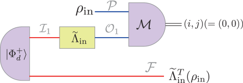
Figure 9: The gate teleportation circuit implements the transposed map Λ~inT\widetilde{\Lambda}_{\mathrm{in}}^{T} for any CPTP map Λ~in\widetilde{\Lambda}_{\mathrm{in}} with a success probability psucc=1/(Dd)p_{\mathrm{succ}}=1/(Dd). The quantum state |Φd+|{\Phi_{d}^{+}}\rangle is a maximally entangled state |Φd+d1/2i=0d1|i|i|{\Phi_{d}^{+}}\rangle\coloneqq d^{-1/2}\sum_{i=0}^{d-1}|{i}\rangle\otimes|{i}\rangle and the POVM \mathcal{M} is the Bell measurement. This protocol succeeds when the measurement outcome of \mathcal{M} is (i,j)=(0,0)(i,j)=(0,0).

Concatenating the protocol for the pseudo complex conjugate map 𝒱~′′\widetilde{\mathcal{V}}^{\prime\prime} and the variant of gate teleportation shown in Figure 9, we obtain an isometry inversion protocol, whose success probability is psucc=1/[Dd(Dd+1)]p_{\mathrm{succ}}=1/[Dd(D-d+1)]. This success probability is less than that of a protocol shown in Figure 2 (c). In general, the success probability of any isometry inversion protocol that is a concatenation of an isometry pseudo complex conjugation protocol and the variant of the gate teleportation shown in Figure 9 is bounded by psucc1/(Dd)p_{\mathrm{succ}}\leq 1/(Dd) since the success probability of the variant of the gate teleportation is 1/(Dd)1/(Dd).

5 Numerical optimization of success probabilities by semidefinite programming

In the preceding sections, we analytically investigated the success probability of parallel protocols for higher-order quantum transformations of isometry operations. Though parallel protocol is efficient in terms of the circuit depth compared to other protocols such as sequential ones, more general strategies than parallel protocols can possibly improve the success probability by utilizing the temporal resource. To analyze this possibility, we perform a numerical optimization of the success probability of isometry inversion, isometry (pseudo) complex conjugation, and isometry transposition by semidefinite programming (SDP) in the same way as presented in Ref. [19] (see Appendix F for the detail). In addition to parallel protocols, we also consider sequential protocols shown in Figure 10 (a) and the most general protocols, which include the cases with an indefinite causal order [70, 71, 72, 73, 74, 75, 76].

To construct efficient sequential protocols for isometry inversion, we also consider the “success-or-draw” version [81] of an isometry inversion protocol shown in Figure 10 (b). As we define in Section 2.2, we say that a superinstrument {𝒮~~,~~}\{{\mathchoice{\widetilde{\hbox{$\displaystyle\widetilde{\mathcal{S}}$}}}{\widetilde{\hbox{$\textstyle\widetilde{\mathcal{S}}$}}}{\widetilde{\hbox{$\scriptstyle\widetilde{\mathcal{S}}$}}}{\widetilde{\hbox{$\scriptscriptstyle\widetilde{\mathcal{S}}$}}}},{\mathchoice{\widetilde{\hbox{$\displaystyle\widetilde{\mathcal{F}}$}}}{\widetilde{\hbox{$\textstyle\widetilde{\mathcal{F}}$}}}{\widetilde{\hbox{$\scriptstyle\widetilde{\mathcal{F}}$}}}{\widetilde{\hbox{$\scriptscriptstyle\widetilde{\mathcal{F}}$}}}}\} implements a probabilistic isometry inversion protocol if the element for the success case 𝒮~~{\mathchoice{\widetilde{\hbox{$\displaystyle\widetilde{\mathcal{S}}$}}}{\widetilde{\hbox{$\textstyle\widetilde{\mathcal{S}}$}}}{\widetilde{\hbox{$\scriptstyle\widetilde{\mathcal{S}}$}}}{\widetilde{\hbox{$\scriptscriptstyle\widetilde{\mathcal{S}}$}}}} satisfies

𝒮~~(𝒱~k)=p𝒱~inv,\displaystyle{\mathchoice{\widetilde{\hbox{$\displaystyle\widetilde{\mathcal{S}}$}}}{\widetilde{\hbox{$\textstyle\widetilde{\mathcal{S}}$}}}{\widetilde{\hbox{$\scriptstyle\widetilde{\mathcal{S}}$}}}{\widetilde{\hbox{$\scriptscriptstyle\widetilde{\mathcal{S}}$}}}}(\widetilde{\mathcal{V}}^{\otimes k})=p\widetilde{\mathcal{V}}_{\mathrm{inv}}, (67)

or equivalently,

𝒮~~(𝒱~k)𝒱~=p𝟙~d\displaystyle{\mathchoice{\widetilde{\hbox{$\displaystyle\widetilde{\mathcal{S}}$}}}{\widetilde{\hbox{$\textstyle\widetilde{\mathcal{S}}$}}}{\widetilde{\hbox{$\scriptstyle\widetilde{\mathcal{S}}$}}}{\widetilde{\hbox{$\scriptscriptstyle\widetilde{\mathcal{S}}$}}}}(\widetilde{\mathcal{V}}^{\otimes k})\circ\widetilde{\mathcal{V}}=p\widetilde{\mathds{1}}_{d} (68)

for all V𝕍iso(d,D)V\in\mathbb{V}_{\mathrm{iso}}(d,D). No extra condition is required for the element for the fail case ~~{\mathchoice{\widetilde{\hbox{$\displaystyle\widetilde{\mathcal{F}}$}}}{\widetilde{\hbox{$\textstyle\widetilde{\mathcal{F}}$}}}{\widetilde{\hbox{$\scriptstyle\widetilde{\mathcal{F}}$}}}{\widetilde{\hbox{$\scriptscriptstyle\widetilde{\mathcal{F}}$}}}} as long as {𝒮~~,~~}\{{\mathchoice{\widetilde{\hbox{$\displaystyle\widetilde{\mathcal{S}}$}}}{\widetilde{\hbox{$\textstyle\widetilde{\mathcal{S}}$}}}{\widetilde{\hbox{$\scriptstyle\widetilde{\mathcal{S}}$}}}{\widetilde{\hbox{$\scriptscriptstyle\widetilde{\mathcal{S}}$}}}},{\mathchoice{\widetilde{\hbox{$\displaystyle\widetilde{\mathcal{F}}$}}}{\widetilde{\hbox{$\textstyle\widetilde{\mathcal{F}}$}}}{\widetilde{\hbox{$\scriptstyle\widetilde{\mathcal{F}}$}}}{\widetilde{\hbox{$\scriptscriptstyle\widetilde{\mathcal{F}}$}}}}\} forms a superinstrument. In general, if the protocol fails, namely, obtaining the outcome corresponding to the fail case ~~{\mathchoice{\widetilde{\hbox{$\displaystyle\widetilde{\mathcal{F}}$}}}{\widetilde{\hbox{$\textstyle\widetilde{\mathcal{F}}$}}}{\widetilde{\hbox{$\scriptstyle\widetilde{\mathcal{F}}$}}}{\widetilde{\hbox{$\scriptscriptstyle\widetilde{\mathcal{F}}$}}}}, the input state ρin\rho_{\mathrm{in}} is destroyed. Therefore this type of “success-or-fail” probabilistic protocols cannot be repeated or sequentially combined with another protocol.
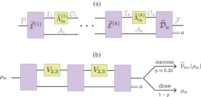
Figure 10: (a) A quantum circuit representation of a sequential superinstrument, where Λ~in(i)(i{1,,k})\widetilde{\Lambda}_{\mathrm{in}}^{(i)}\;(i\in\{1,\cdots,k\}) are input maps, ~(i)(i{1,,k})\widetilde{\mathcal{E}}^{(i)}\;(i\in\{1,\cdots,k\}) are CPTP maps, and {𝒟~a}\{\widetilde{\mathcal{D}}_{a}\} is a quantum instrument. (b) A quantum circuit representation of a sequential “success-or-draw” protocol for isometry inversion of V𝕍iso(2,3)V\in\mathbb{V}_{\mathrm{iso}}(2,3). For the input quantum state ρin(ImV)\rho_{\mathrm{in}}\in\mathcal{L}(\mathrm{Im}V), we obtain the output quantum state given by 𝒱~inv(ρin)\widetilde{\mathcal{V}}_{\mathrm{inv}}(\rho_{\mathrm{in}}) after success or the output quantum state given by ρin\rho_{\mathrm{in}} after a draw. The optimal success probability p0.33p\approx 0.33 is obtained by the SDP for d=2d=2, D=3D=3 and k=2k=2.

For the “success-or-draw” version of an isometry inversion protocol, we impose an additional condition on ~~{\mathchoice{\widetilde{\hbox{$\displaystyle\widetilde{\mathcal{F}}$}}}{\widetilde{\hbox{$\textstyle\widetilde{\mathcal{F}}$}}}{\widetilde{\hbox{$\scriptstyle\widetilde{\mathcal{F}}$}}}{\widetilde{\hbox{$\scriptscriptstyle\widetilde{\mathcal{F}}$}}}} given by

~~(𝒱~k)𝒱~=(1p)𝒱~\displaystyle{\mathchoice{\widetilde{\hbox{$\displaystyle\widetilde{\mathcal{F}}$}}}{\widetilde{\hbox{$\textstyle\widetilde{\mathcal{F}}$}}}{\widetilde{\hbox{$\scriptstyle\widetilde{\mathcal{F}}$}}}{\widetilde{\hbox{$\scriptscriptstyle\widetilde{\mathcal{F}}$}}}}(\widetilde{\mathcal{V}}^{\otimes k})\circ\widetilde{\mathcal{V}}=(1-p)\widetilde{\mathcal{V}} (69)

for all V𝕍iso(d,D)V\in\mathbb{V}_{\mathrm{iso}}(d,D). This condition means that even after the protocol fails, we recover the original input state as the output of the protocol if the input state is in the image ImV\mathrm{Im}V of the input isometry operator V𝕍iso(d,D)V\in\mathbb{V}_{\mathrm{iso}}(d,D). Such a type of failure is called a draw because the protocol can be repeated after failure. By repeating the “success-or-draw” protocol until success at most mm times, we can achieve the probability given by psucc=1(1p)mp_{\mathrm{succ}}=1-(1-p)^{m}. In other words, the failure probability 1psucc1-p_{\mathrm{succ}} decreases exponentially with the number k=mkk^{\prime}=mk of calls of an input isometry operation. Therefore, the number of calls of an input isometry operation scales logarithmically with respect to the success probability, i.e., k=𝒪(ln(1/(1psucc)))k^{\prime}=\mathcal{O}(\ln(1/(1-p_{\mathrm{succ}}))). We perform the SDP to obtain such a “success-or-draw” protocol for isometry inversion in a similar way as presented in Ref. [81] (see Appendix F for the detail).

isometry inversion
d=2,D=3d=2,D=3 parallel sequential general
k=1k=1 0.250.25 0.250.25 0.250.25
k=2k=2 0.40.4 0.42863/70.4286\approx 3/7 0.42863/70.4286\approx 3/7
isometry complex conjugation
d=2,D=3d=2,D=3 parallel sequential general
k3k\leq 3 0 0 0
isometry pseudo complex conjugation
d=2,D=3d=2,D=3 parallel sequential general
k=1k=1 0.50001/20.5000\approx 1/2 0.50001/20.5000\approx 1/2 0.50001/20.5000\approx 1/2
k=2k=2 0.5453 0.5453 0.5453
d=2,D=4d=2,D=4 parallel sequential general
k=1k=1 0.33331/30.3333\approx 1/3 0.33331/30.3333\approx 1/3 0.33331/30.3333\approx 1/3
isometry transposition
d=2,D=3d=2,D=3 parallel sequential general
k=1k=1 1/61/6 1/61/6 1/61/6
k=2k=2 0.28572/70.2857\approx 2/7 0.30770.3077 0.33331/30.3333\approx 1/3
d=2,D=4d=2,D=4 parallel sequential general
k=1k=1 0.1250.125 0.1250.125 0.1250.125
k=2k=2 0.222/90.22\approx 2/9 - -
Table 1: The optimal success probabilities of isometry inversion, (pseudo) complex conjugation, and transposition using kk calls of an input isometry operation 𝒱~\widetilde{\mathcal{V}} corresponding to V𝕍iso(d,D)V\in\mathbb{V}_{\mathrm{iso}}(d,D). The bold values are obtained analytically.
unitary inversion
d=2d=2 parallel sequential general
k=1k=1 0.250.25 0.250.25 0.250.25
k=2k=2 0.40.4 0.42863/70.4286\approx 3/7 0.44444/90.4444\approx 4/9
Table 2: The optimal success probability of unitary inversion using kk calls of an input unitary operation 𝒰~\widetilde{\mathcal{U}} corresponding to U𝕌(d)U\in\mathbb{U}(d) derived in Ref. [18].

Table 1 and Figure 10 (b) show the results of the SDP optimization. Table 2 shows the optimal success probability of unitary inversion, which was already obtained in Ref. [18], for the comparison with that of isometry inversion. We implement the SDP code in MATLAB [82] by modifying the SDP code [83] accompanied Refs. [18, 19], originally designed to obtain the optimal success probability of unitary inversion and unitary transposition. The interpreters CVX [84, 85] and YALMIP [86, 87] are used with the solvers SDPT3 [88, 89, 90], SeDuMi [91], MOSEK [92] and SCS [93] to perform the SDP. The code also uses functions in QETLAB [94]. All codes to obtain the results shown in Table 1 and Figure 10 (b) are available at Ref. [95] under the MIT license [96].

First, we consider isometry inversion. Theorem 1 shows that the optimal success probability of probabilistic parallel isometry inversion protocols using kk calls of an input isometry operation corresponding to V𝕍iso(d,D)V\in\mathbb{V}_{\mathrm{iso}}(d,D) is equal to that of probabilistic parallel unitary inversion protocols using kk calls of an input unitary operation corresponding to U𝕌(d)U\in\mathbb{U}(d). This statement can be also checked numerically for d=2d=2, D=3D=3 and k{1,2}k\in\{1,2\} by comparing Table 1 with Table 2. Comparison of Table 1 with Table 2 also shows that the optimal success probability of sequential isometry inversion is the same as that of sequential unitary inversion for d=2d=2, D=3D=3 and k=2k=2. This numerical result implies the possibility that the optimal success probability of kk-input sequential protocols for isometry inversion of V𝕍iso(d,D)V\in\mathbb{V}_{\mathrm{iso}}(d,D) does not depend on DD.

We also numerically confirmed the existence of a sequential “success-or-draw” protocol for isometry inversion for d=2d=2, D=3D=3 and k=2k=2 by the SDP (see Figure 10 (b)). By repeating this “success-or-draw” protocol, we can implement a sequential protocol for isometry inversion with the success probability scaling as psucc=1exp[𝒪(k)]p_{\mathrm{succ}}=1-\exp[-\mathcal{O}(k)]. In contrast, we can show the upper bound of the success probability of any parallel protocol for isometry inversion given by psucc1𝒪(k1)p_{\mathrm{succ}}\leq 1-\mathcal{O}(k^{-1}) from the same upper bound for unitary inversion presented in Ref. [18]. Thus an exponential improvement of the success probability of a sequential protocol for isometry inversion compared to a parallel protocol for d=2d=2 and D=3D=3 is exhibited. However, a further general protocol does not improve the success probability of isometry inversion compared to a sequential protocol for d=2d=2, D=3D=3 and k=2k=2 as shown numerically in Table 1, whereas an improvement with a general protocol was observed for the case of d=2d=2 and k=2k=2 unitary inversion as shown in Table 2.

Next, we consider isometry complex conjugation. Theorem 5 shows that it is impossible to transform finite calls of an isometry operation 𝒱~:(d)(D)\widetilde{\mathcal{V}}:\mathcal{L}(\mathbb{C}^{d})\to\mathcal{L}(\mathbb{C}^{D}) into its complex conjugate map 𝒱~\widetilde{\mathcal{V}}^{*} with a non-zero success probability for D2dD\geq 2d. In addition to this theorem, the numerical result in Table 1 indicates that it is also impossible for d=2,D=3d=2,D=3 and k{1,2,3}k\in\{1,2,3\}, although D2dD\geq 2d is not satisfied. This result implies the possibility that probabilistic isometry complex conjugation is impossible even for d<D<2dd<D<2d.

Then, we consider isometry pseudo complex conjugation. The numerical result shown in Table 1 indicates that the optimal success probability of isometry pseudo complex conjugation is equal to the success probability psucc=1/(Dd+1)p_{\mathrm{succ}}=1/(D-d+1) of a parallel protocol shown in Figure 8 for d=2d=2, D{3,4}D\in\{3,4\} and k=d1=1k=d-1=1. The numerical result also shows that a parallel protocol achieves the optimal success probability of isometry pseudo complex conjugation among general protocols including indefinite causal order for d=2d=2, D=3D=3 and k=2k=2.

Finally, we consider isometry transposition (see also Appendix E). The numerical result shown in Table 1 indicates that the optimal success probability of parallel isometry transposition is equal to the success probability psucc=k/(Dd+k1)p_{\mathrm{succ}}=k/(Dd+k-1) of a protocol shown in Figure 12 for d=2d=2, D{3,4}D\in\{3,4\} and k=2k=2. This result implies the possibility that a protocol shown in Figure 12 achieves the optimal success probability for any choice of dd, DD and kk. The numerical result also shows that a sequential protocol and a general protocol can improve the success probability of isometry transposition in contrast to the case of isometry inversion.

We present a conjecture and open problems obtained from the discussion for the SDP optimization results.

Conjecture: The optimal success probability of probabilistic parallel protocols that transform kk calls of an isometry operation 𝒱~\widetilde{\mathcal{V}} corresponding to V𝕍iso(d,D)V\in\mathbb{V}_{\mathrm{iso}}(d,D) into its transposed map 𝒱~T\widetilde{\mathcal{V}}^{T} is psucc=k/(Dd+k1)p_{\mathrm{succ}}=k/(Dd+k-1), which is achieved by the protocol shown in Figure 12.

Open problem 1: Does the optimal success probability of sequential isometry inversion depend on DD?

Open problem 2: Does indefinite causal order improve the success probability of isometry inversion?

Open problem 3: Is it possible to transform finite calls of an isometry operation 𝒱~\widetilde{\mathcal{V}} corresponding to V𝕍iso(d,D)V\in\mathbb{V}_{\mathrm{iso}}(d,D) into its complex conjugate map 𝒱~\widetilde{\mathcal{V}}^{*} with a non-zero success probability for d<D<2dd<D<2d?

6 Conclusion

We presented a probabilistic exact parallel protocol for isometry inversion that constructs a decoder from multiple calls of a black box encoder implementing an unknown isometry operation transforming a dd-dimensional system to a DD-dimensional system for D>dD>d. The success probability of this protocol is independent of DD. Thus, this protocol significantly outperforms other isometry inversion protocols that use DD-dimensional unitary inversion protocols or quantum process tomography of isometry operations for DdD\gg d. This shows a potential of our protocol for applications in quantum information processing involving encoding and decoding with black boxes. In particular, we consider a typical example of an encoding black box represented by an isometry operation to spread quantum information of a qudit (a dd-dimensional system) into a nn-qudit system (a dnd^{n}-dimensional system). It may seem that inverting the function from a black box function is difficult due to the exponential dimensionality of dnd^{n} of isometry operations, but our result shows that such an implementation is easy whenever dd is small enough.

We developed a new technique to construct isometry inversion protocols, since the strategy for unitary inversion used in the previous work [18] is not applicable to isometry inversion. This is because the probabilistic exact isometry complex conjugation is impossible for D2dD\geq 2d, and the concatenation of isometry pseudo complex conjugation and a variant of the gate teleportation is inefficient. Then, we showed the decomposition of the tensor product of an isometry and invent a CPTP map Ψ~\widetilde{\Psi} that can be implemented by the quantum Schur transform [77, 78, 79] and the “measure-and-prepare” strategy [64, 3]. This CPTP map transforms k+1k+1 parallel calls of an isometry operation into the Haar integral of k+1k+1 tensor product of unitary operations as shown in Eq. (23) of Lemma 4, which contributes to keeping the dimension dependence of the success probability to dd and independent of DD. This technique provides a new application of the quantum Schur transform, which is known to have various applications to quantum information processing [77].

We also performed the SDP to investigate the improvement of the success probability of a sequential protocol or a protocol with indefinite causal order for isometry inversion, isometry complex conjugation and isometry transposition compared to a parallel protocol. From the numerical calculation, we found a “success-or-draw” isometry inversion protocol for d=2d=2 and D=3D=3. By repeating this protocol, we can obtain a sequential protocol for isometry inversion with a failure probability decreasing exponentially with the number of calls of the input isometry operation. This result exhibits an exponential improvement of the success probability of a sequential protocol for isometry inversion for d=2d=2 and D=3D=3 compared to a parallel protocol.

Acknowledgements.
The authors thank M. T. Quintino for inspiring discussions, especially for pointing out the relationship between the uniqueness of isometry transposition and the optimality of the success probability. We also thank an anonymous reviewer of Quantum for providing a resource evaluation of process tomography of isometry operations. This work was supported by MEXT Quantum Leap Flagship Program (MEXT QLEAP) Grant No. JPMXS0118069605, JPMXS0120351339, Japan Society for the Promotion of Science (JSPS) KAKENHI Grant No. 18K13467, 21H03394 and the Forefront Physics and Mathematics Program to Drive Transformation (FoPM) of the University of Tokyo.

Appendix A Higher-order quantum transformations

Choi-Jamiolkowski (CJ) isomorphism is a useful tool for treating linear maps as operators called Choi operators by “lowering” the order of transformations. Similarly, the CJ isomorphism is used for describing higher-order quantum transformations by Choi operators of higher-order quantum transformation. We summarize the formulation of linear maps and higher-order quantum transformations using the Choi operators.

Any linear map Λ~:()(𝒪)\widetilde{\Lambda}:\mathcal{L}(\mathcal{I})\to\mathcal{L}(\mathcal{O}) can be represented uniquely by the Choi operator defined by

JΛ~i,j|ij|Λ~(|ij|)𝒪(𝒪),\displaystyle J_{\widetilde{\Lambda}}\coloneqq\sum_{i,j}|{i}\rangle\!\langle{j}|_{\mathcal{I}}\otimes\widetilde{\Lambda}(|{i}\rangle\!\langle{j}|)_{\mathcal{O}}\in\mathcal{L}(\mathcal{I}\otimes\mathcal{O}), (70)

where {|i}\{|{i}\rangle\} is an orthonormal basis in \mathcal{I}. The map Λ~\widetilde{\Lambda} can be obtained from JΛ~J_{\widetilde{\Lambda}} as

Λ~(ρ)=Tr[JΛ~(ρT𝟙𝒪)],\displaystyle\widetilde{\Lambda}(\rho_{\mathcal{I}})={\mathrm{Tr}}_{\mathcal{I}}[J_{\widetilde{\Lambda}}(\rho_{\mathcal{I}}^{T}\otimes\mathds{1}_{\mathcal{O}})], (71)

where ρT\rho_{\mathcal{I}}^{T} is the transposition of an input quantum state ρ\rho_{\mathcal{I}} in the computational basis.

A CPTP map Λ~\widetilde{\Lambda} can be characterized in terms of its Choi operator. First, we consider a CP map Λ~\widetilde{\Lambda} and let {Kk}:𝒪\{K_{k}\}:\mathcal{I}\to\mathcal{O} be its Kraus operators, i.e., Λ~(ρ)=kKkρKk\widetilde{\Lambda}(\rho)=\sum_{{k}}K_{k}\rho K_{k}^{\dagger}. Then, its Choi operator is given by

JΛ~=k|KkKk|,\displaystyle J_{\widetilde{\Lambda}}=\sum_{k}|{K_{k}}\rangle\!\rangle\!\langle\!\langle{K_{k}}|, (72)

where |Kk|{K_{k}}\rangle\!\rangle is a vector representing a rank-1 Choi vector defined as |Kki|i(Kk|i)𝒪𝒪|{K_{k}}\rangle\!\rangle\coloneqq\sum_{i}|{i}\rangle_{\mathcal{I}}\otimes(K_{k}|{i}\rangle)_{\mathcal{O}}\in\mathcal{I}\otimes\mathcal{O}, also referred to as a dual ket vector. Since JΛ~J_{\widetilde{\Lambda}} is represented by a sum of rank-1 positive operators, it is a positive operator. Conversely, if JΛ~J_{\widetilde{\Lambda}} is positive, JΛ~J_{\widetilde{\Lambda}} can be written in the form of Eq. (72). Then, Λ~(ρ)=kKkρKk\widetilde{\Lambda}(\rho)=\sum_{{k}}K_{k}\rho K_{k}^{\dagger}, which means that Λ~\widetilde{\Lambda} is a CP map. Therefore, Λ~\widetilde{\Lambda} is CP if and only if its Choi operator JΛ~J_{\widetilde{\Lambda}} is positive. Next, a map Λ~\widetilde{\Lambda} is TP if and only if Tr𝒪Λ~(|ij|)=δi,j{\mathrm{Tr}}_{\mathcal{O}}\widetilde{\Lambda}(|{i}\rangle\!\langle{j}|)=\delta_{i,j} for all i,ji,j. Therefore, Λ~\widetilde{\Lambda} is TP if and only if Tr𝒪JΛ~=I{\mathrm{Tr}}_{\mathcal{O}}J_{\widetilde{\Lambda}}=I_{\mathcal{I}}. Similarly, a quantum instrument is represented by a set of CP maps {Λ~a}\{\widetilde{\Lambda}_{a}\} and it can be also characterized by the corresponding set of Choi operators {JΛ~a}\{J_{\widetilde{\Lambda}_{a}}\}.

The composition of two maps can be represented by a link product denoted by \star. Let X(𝒳𝒴)X\in\mathcal{L}(\mathcal{X}\otimes\mathcal{Y}) and Y(𝒴𝒵)Y\in\mathcal{L}(\mathcal{Y}\otimes\mathcal{Z}). The link product of XX and YY is defined as

YXTr[(𝟙𝒳Y)(XT𝒴𝟙𝒵)],\displaystyle Y\star X\coloneqq{\mathrm{Tr}}_{\mathcal{H}}[(\mathds{1}_{\mathcal{X}}\otimes Y)(X^{T_{\mathcal{Y}}}\otimes\mathds{1}_{\mathcal{Z}})], (73)

where XT𝒴X^{T_{\mathcal{Y}}} is the partial transpose of XX on 𝒴\mathcal{Y}. We consider two maps Λ~1:(1)(2)\widetilde{\Lambda}_{1}:\mathcal{L}(\mathcal{I}_{1})\to\mathcal{L}(\mathcal{I}_{2}) and Λ~2:(2)(𝒪1)\widetilde{\Lambda}_{2}:\mathcal{L}(\mathcal{I}_{2})\to\mathcal{L}(\mathcal{O}_{1}). The Choi operator of Λ~2Λ~1\widetilde{\Lambda}_{2}\circ\widetilde{\Lambda}_{1} is obtained by

JΛ~2Λ~1=JΛ~2JΛ~1.\displaystyle J_{\widetilde{\Lambda}_{2}\circ\widetilde{\Lambda}_{1}}=J_{\widetilde{\Lambda}_{2}}\star J_{\widetilde{\Lambda}_{1}}. (74)

Similarly to CPTP maps and quantum instruments, higher order-quantum transformations can be represented by Choi operators. In particular, we use the Choi operator representation of a single-input superinstrument for the analysis in this paper. A single-input superinstrument {𝒞~~a}\{{\mathchoice{\widetilde{\hbox{$\displaystyle\widetilde{\mathcal{C}}$}}}{\widetilde{\hbox{$\textstyle\widetilde{\mathcal{C}}$}}}{\widetilde{\hbox{$\scriptstyle\widetilde{\mathcal{C}}$}}}{\widetilde{\hbox{$\scriptscriptstyle\widetilde{\mathcal{C}}$}}}}_{a}\} can be characterized by the corresponding set of Choi operators {Ca}\{C_{a}\} as

Ca\displaystyle C_{a} 0,\displaystyle\geq 0, (75)
TrC\displaystyle{\mathrm{Tr}}_{\mathcal{F}}C =Tr𝒪C𝟙𝒪d𝒪,\displaystyle={\mathrm{Tr}}_{\mathcal{FO}}C\otimes\frac{\mathds{1}_{\mathcal{O}}}{d_{\mathcal{O}}}, (76)
Tr𝒪C\displaystyle{\mathrm{Tr}}_{\mathcal{FOI}}C =TrC𝟙𝒫d𝒫,\displaystyle={\mathrm{Tr}}C\otimes\frac{\mathds{1}_{\mathcal{P}}}{d_{\mathcal{P}}}, (77)
TrC\displaystyle{\mathrm{Tr}}C =d𝒫d𝒪,\displaystyle=d_{\mathcal{P}}d_{\mathcal{O}}, (78)

where CC is defined as CaCaC\coloneqq\sum_{{a}}C_{a} [55]. The Choi operators {Ca}\{C_{a}\} are related to the corresponding single-input superinstrument {𝒞~~a}\{{\mathchoice{\widetilde{\hbox{$\displaystyle\widetilde{\mathcal{C}}$}}}{\widetilde{\hbox{$\textstyle\widetilde{\mathcal{C}}$}}}{\widetilde{\hbox{$\scriptstyle\widetilde{\mathcal{C}}$}}}{\widetilde{\hbox{$\scriptscriptstyle\widetilde{\mathcal{C}}$}}}}_{a}\} as

CaJΛ~in=J𝒞~~a(Λ~in).\displaystyle C_{a}\star J_{\widetilde{\Lambda}_{\mathrm{in}}}=J_{{\mathchoice{\widetilde{\hbox{$\displaystyle\widetilde{\mathcal{C}}$}}}{\widetilde{\hbox{$\textstyle\widetilde{\mathcal{C}}$}}}{\widetilde{\hbox{$\scriptstyle\widetilde{\mathcal{C}}$}}}{\widetilde{\hbox{$\scriptscriptstyle\widetilde{\mathcal{C}}$}}}}_{a}(\widetilde{\Lambda}_{\mathrm{in}})}. (79)

See Ref. [97] for the characterization of kk-input superinstruments.

Appendix B Extension of the Schur-Weyl duality to the decomposition of the tensor product of isometry operators

We first review the Schur-Weyl duality. We consider Hilbert spaces 𝒳i=d\mathcal{X}_{i}=\mathbb{C}^{d} for i{1,,k}i\in\{1,\cdots,k\} and define the joint Hilbert space by 𝒳i=1k𝒳i\mathcal{X}\coloneqq\bigotimes_{i=1}^{k}\mathcal{X}_{i}. We consider representations of the unitary group 𝕌(d)\mathbb{U}(d) and the symmetric group 𝔖k\mathfrak{S}_{k} defined as

𝕌(d)\displaystyle\mathbb{U}(d)\to (𝒳);UUk,\displaystyle\mathcal{L}(\mathcal{X});\;\;\;U\mapsto U^{\otimes k}, (80)
𝔖k\displaystyle\mathfrak{S}_{k}\to (𝒳);σPσ,\displaystyle\mathcal{L}(\mathcal{X});\;\;\;\sigma\mapsto P_{\sigma}, (81)

where PσP_{\sigma} is the permutation operator defined by

Pσ(i=1k|ψi)=i=1k|ψσ1(i).\displaystyle P_{\sigma}\left(\bigotimes_{i=1}^{k}|{\psi_{i}}\rangle\right)=\bigotimes_{i=1}^{k}|{\psi_{\sigma^{-1}(i)}}\rangle. (82)

These representations can be decomposed as

𝒳\displaystyle\mathcal{X} =μk𝒰μ,𝒳(d)𝒮μ,𝒳(k),\displaystyle=\bigoplus_{\mu\vdash k}\mathcal{U}_{\mu,\mathcal{X}}^{(d)}\otimes\mathcal{S}_{\mu,\mathcal{X}}^{(k)}, (83)
Uk\displaystyle U^{\otimes k} =μkUμ𝟙𝒮μ,𝒳(k),\displaystyle=\bigoplus_{\mu\vdash k}U_{\mu}\otimes\mathds{1}_{\mathcal{S}_{\mu,\mathcal{X}}^{(k)}}, (84)
Pσ\displaystyle P_{\sigma} =μk𝟙𝒰μ,𝒳(d)Pσ,μ,\displaystyle=\bigoplus_{\mu\vdash k}\mathds{1}_{\mathcal{U}_{\mu,\mathcal{X}}^{(d)}}\otimes P_{\sigma,\mu}, (85)

where the summands are indexed by the Young diagrams μ\mu with kk boxes, 𝕌(d)UUμ(𝒰μ,𝒳(d))\mathbb{U}(d)\ni U\mapsto U_{\mu}\in\mathcal{L}(\mathcal{U}_{\mu,\mathcal{X}}^{(d)}) are irreducible representations of 𝕌(D)\mathbb{U}(D), 𝔖kσPσ,μ(𝒮μ,𝒳(k))\mathfrak{S}_{k}\ni\sigma\mapsto P_{\sigma,\mu}\in\mathcal{L}(\mathcal{S}_{\mu,\mathcal{X}}^{(k)}) are irreducible representations of 𝔖k\mathfrak{S}_{k} and 𝟙𝒮μ,𝒳(k)\mathds{1}_{\mathcal{S}_{\mu,\mathcal{X}}^{(k)}} and 𝟙𝒰μ,𝒳(d)\mathds{1}_{\mathcal{U}_{\mu,\mathcal{X}}^{(d)}} are the identity operators on 𝒮μ,𝒳(k)\mathcal{S}_{\mu,\mathcal{X}}^{(k)} and 𝒰μ,𝒳(d)\mathcal{U}_{\mu,\mathcal{X}}^{(d)}, respectively [98]. The dimension of 𝒰μ,𝒳(d)\mathcal{U}_{\mu,\mathcal{X}}^{(d)} is non-zero if and only if μ\mu has at most kk rows, and 𝒰μ,𝒳(d)\mathcal{U}_{\mu,\mathcal{X}}^{(d)} and 𝒮μ,𝒳(k)\mathcal{S}_{\mu,\mathcal{X}}^{(k)} are spanned by bases called the Gel’fand-Zetlin basis and the Young orthonormal basis [79, 99], respectively. Each element in the Gel’fand-Zetlin basis and the Young orthonormal basis is labeled by a semi-standard tableau uμu_{\mu} and a standard tableau sμs_{\mu} whose frame is μ\mu, respectively. In total, the Hilbert space 𝒳\mathcal{X} is spanned by the set of vectors {|μ,uμ,sμ}\{|{\mu,u_{\mu},s_{\mu}}\rangle\}, which is called the Schur basis.

We extend the Schur-Weyl duality to show the decomposition of the tensor product of isometry operators. We consider Hilbert spaces 𝒴i=D\mathcal{Y}_{i}=\mathbb{C}^{D} for i{1,,k}i\in\{1,\cdots,k\} and define the joint Hilbert space 𝒴\mathcal{Y} by 𝒴i=1k𝒴i\mathcal{Y}\coloneqq\bigotimes_{i=1}^{k}\mathcal{Y}_{i}. We consider the tensor product Vk:𝒳𝒴V^{\otimes k}:\mathcal{X}\to\mathcal{Y} of an isometry operator V𝕍iso(d,D)V\in\mathbb{V}_{\mathrm{iso}}(d,D). We decompose VkV^{\otimes k} in the Schur basis as

Vk=μ,μkl(μ)d,l(μ)DαAμ,μαBμ,μα,\displaystyle V^{\otimes k}=\bigoplus_{\begin{subarray}{c}\mu,\mu^{\prime}\vdash k\\ l(\mu)\leq d,l(\mu^{\prime})\leq D\end{subarray}}\sum_{\alpha}A^{\alpha}_{\mu,\mu^{\prime}}\otimes B^{\alpha}_{\mu,\mu^{\prime}}, (86)

where l(μ)l(\mu) is the number of rows of a Young diagram μ\mu, {Aμ,μα}\{A^{\alpha}_{\mu,\mu^{\prime}}\} is a basis of the set of linear operators (𝒰μ,𝒳(d)𝒰μ,𝒴(D))\mathcal{L}(\mathcal{U}^{(d)}_{\mu,\mathcal{X}}\to\mathcal{U}^{(D)}_{\mu^{\prime},\mathcal{Y}}) and Bμ,μαB^{\alpha}_{\mu,\mu^{\prime}} is a linear operator Bμ,μα:𝒮μ,𝒳(k)𝒮μ,𝒴(k)B^{\alpha}_{\mu,\mu^{\prime}}:\mathcal{S}^{(k)}_{\mu,\mathcal{X}}\to\mathcal{S}^{(k)}_{\mu^{\prime},\mathcal{Y}}. Since VkV^{\otimes k} is invariant under the action of the symmetric group 𝔖k\mathfrak{S}_{k}, i.e.,

Pσ,𝒴VkPσ,𝒳=Vk\displaystyle P_{\sigma,\mathcal{Y}}^{\dagger}V^{\otimes k}P_{\sigma,\mathcal{X}}=V^{\otimes k} (87)

holds for all σ𝔖k\sigma\in\mathfrak{S}_{k},

Pσ,μBμ,μαPσ,μ=Bμ,μα\displaystyle P_{\sigma,\mu^{\prime}}^{\dagger}B^{\alpha}_{\mu,\mu^{\prime}}P_{\sigma,\mu}=B^{\alpha}_{\mu,\mu^{\prime}} (88)

holds for all μ,μk\mu,\mu^{\prime}\vdash k and σ𝔖k\sigma\in\mathfrak{S}_{k}. From Schur’s lemma, if μ=μ\mu=\mu^{\prime} (i.e., the irreducible representations 𝒮μ,𝒳(k)\mathcal{S}^{(k)}_{\mu,\mathcal{X}} and 𝒮μ,𝒴(k)\mathcal{S}^{(k)}_{\mu^{\prime},\mathcal{Y}} are unitarily equivalent), Bμ,μαB^{\alpha}_{\mu,\mu^{\prime}} is the isomorphism between the irreducible representations 𝒮μ,𝒳(k)\mathcal{S}^{(k)}_{\mu,\mathcal{X}} and 𝒮μ,𝒴(k)\mathcal{S}^{(k)}_{\mu^{\prime},\mathcal{Y}}, and if μμ\mu\neq\mu^{\prime}, Bμ,μα=0B^{\alpha}_{\mu,\mu^{\prime}}=0. Note that the isomorphism between the irreducible representations of the symmetric group is unique up to a constant multiplication. Thus, we obtain the decomposition of VkV^{\otimes k} given by

Vk=μkl(μ)dVμI𝒮μ,𝒳(k)𝒮μ,𝒴(k),\displaystyle V^{\otimes k}=\bigoplus_{\begin{subarray}{c}\mu\vdash k\\ l(\mu)\leq d\end{subarray}}V_{\mu}\otimes I_{\mathcal{S}_{\mu,\mathcal{X}}^{(k)}\to\mathcal{S}_{\mu,\mathcal{Y}}^{(k)}}, (89)

where Vμ(𝒰μ,𝒳(d)𝒰μ,𝒴(D))V_{\mu}\in\mathcal{L}(\mathcal{U}_{\mu,\mathcal{X}}^{(d)}\to\mathcal{U}_{\mu,\mathcal{Y}}^{(D)}) is a linear operator and I𝒮μ,𝒳(k)𝒮μ,𝒴(k)I_{\mathcal{S}_{\mu,\mathcal{X}}^{(k)}\to\mathcal{S}_{\mu,\mathcal{Y}}^{(k)}} is the isomorphism between irreducible representations 𝒮μ,𝒳(k)\mathcal{S}_{\mu,\mathcal{X}}^{(k)} and 𝒮μ,𝒴(k)\mathcal{S}_{\mu,\mathcal{Y}}^{(k)}, which transforms a basis vector of 𝒮μ,𝒳(k)\mathcal{S}_{\mu,\mathcal{X}}^{(k)} corresponding to a standard tableau into a basis vector of 𝒮μ,𝒴(k)\mathcal{S}_{\mu,\mathcal{Y}}^{(k)} corresponding to the same standard tableau. Since VkV^{\otimes k} and I𝒮μ,𝒳(k)𝒮μ,𝒴(k)I_{\mathcal{S}_{\mu,\mathcal{X}}^{(k)}\to\mathcal{S}_{\mu,\mathcal{Y}}^{(k)}} are isometry operators, VμV_{\mu} is also an isometry operator.

Note that the decomposition of the tensor product of isometric extension VΛ~:𝒜V_{\widetilde{\Lambda}}:\mathcal{A}\to\mathcal{B}\otimes\mathcal{E} of a quantum channel Λ~:(𝒜)()\widetilde{\Lambda}:\mathcal{L}(\mathcal{A})\to\mathcal{L}(\mathcal{B}) is discussed in Ref. [77]. Reference [77] uses the basis of the input space 𝒜k\mathcal{A}^{\otimes k} as the Schur basis, and the basis of the output space ()k(\mathcal{B}\otimes\mathcal{E})^{\otimes k} as the tensor product of the Schur bases of k\mathcal{B}^{\otimes k} and k\mathcal{E}^{\otimes k} to represent the tensor product VΛ~kV_{\widetilde{\Lambda}}^{\otimes k}. However, the expression of VΛ~kV_{\widetilde{\Lambda}}^{\otimes k} is not block diagonal in that basis. In contrast, we show the block diagonal decomposition of the tensor product VkV^{\otimes k} of an isometry operator VV as shown in Eq. (89).

Appendix C Haar measure on the unitary group

The Haar measure dU{\mathrm{d}}U is the uniform measure defined on the set of unitary operators 𝕌(d)\mathbb{U}(d). More precisely, it is uniquely determined by the following properties [100]:

𝑑U\displaystyle\int{\mathrm{d}}U =1,\displaystyle=1, (90)
d(UUU′′)\displaystyle{\mathrm{d}}(U^{\prime}UU^{\prime\prime}) =dU(U,U′′𝕌(D)).\displaystyle={\mathrm{d}}U\;\;\;(\forall U^{\prime},U^{\prime\prime}\in\mathbb{U}(D)). (91)

We consider the action of the Haar random unitary operations on a quantum state. Suppose 𝒳i=d\mathcal{X}_{i}=\mathbb{C}^{d} for i{1,,k}i\in\{1,\cdots,k\} and define the joint Hilbert space by 𝒳=i=1k𝒳i\mathcal{X}=\bigotimes_{i=1}^{k}\mathcal{X}_{i}. For a quantum state ρ(𝒳)\rho\in\mathcal{L}(\mathcal{X}), we define a quantum state ρ(𝒳)\rho^{\prime}\in\mathcal{L}(\mathcal{X}) by

ρdUUkρUk,\displaystyle\rho^{\prime}\coloneqq\int{\mathrm{d}}UU^{\otimes k}\rho U^{\dagger\otimes k}, (92)

where dU{\mathrm{d}}U is the Haar measure on 𝕌(d)\mathbb{U}(d). From Eq. (91), we obtain

[Uk,ρ]=0(U𝕌(D)),\displaystyle[U^{\otimes k},\rho^{\prime}]=0\;\;\;(\forall U\in\mathbb{U}(D)), (93)

where [A,B]ABBA[A,B]\coloneqq AB-BA is a commutator. By Schur’s lemma, the operator ρ\rho^{\prime} satisfies

ρ=μkI𝒰μ,𝒳(d)d𝒰μ(d)X𝒮μ,𝒳(k),\displaystyle\rho^{\prime}=\bigoplus_{\mu\vdash k}\frac{I_{\mathcal{U}_{\mu,\mathcal{X}}^{(d)}}}{d_{\mathcal{U}_{\mu}^{(d)}}}\otimes X_{\mathcal{S}^{(k)}_{\mu,\mathcal{X}}}, (94)

where X𝒮μ,𝒳(k)X_{\mathcal{S}^{(k)}_{\mu,\mathcal{X}}} is a positive operator on 𝒮μ,𝒳(k)\mathcal{S}^{(k)}_{\mu,\mathcal{X}}. The operator X𝒮μ,𝒳(k)X_{\mathcal{S}^{(k)}_{\mu,\mathcal{X}}} is calculated as

X𝒮μ,𝒳(k)\displaystyle X_{\mathcal{S}^{(k)}_{\mu,\mathcal{X}}} =Tr𝒰μ,𝒳(d)(Πμ,𝒳ρ)\displaystyle={\mathrm{Tr}}_{\mathcal{U}^{(d)}_{\mu,\mathcal{X}}}(\Pi_{\mu,\mathcal{X}}\rho^{\prime}) (95)
=dUTr𝒰μ,𝒳(d){Πμ,𝒳[𝒰~μ𝟙~𝒮μ,𝒳(k)(ρ)]}\displaystyle=\int{\mathrm{d}}U{\mathrm{Tr}}_{\mathcal{U}^{(d)}_{\mu,\mathcal{X}}}\left\{\Pi_{\mu,\mathcal{X}}\left[\widetilde{\mathcal{U}}_{\mu}\otimes\widetilde{\mathds{1}}_{\mathcal{S}^{(k)}_{\mu,\mathcal{X}}}(\rho)\right]\right\} (96)
=dUTr𝒰μ,𝒳(d){[𝒰~μ𝟙~𝒮μ,𝒳(k)(Πμ,𝒳)]ρ}\displaystyle=\int{\mathrm{d}}U{\mathrm{Tr}}_{\mathcal{U}^{(d)}_{\mu,\mathcal{X}}}\left\{\left[\widetilde{\mathcal{U}}^{\dagger}_{\mu}\otimes\widetilde{\mathds{1}}_{\mathcal{S}^{(k)}_{\mu,\mathcal{X}}}(\Pi_{\mu,\mathcal{X}})\right]\rho\right\} (97)
=dUTr𝒰μ,𝒳(d)(Πμ,𝒳ρ)\displaystyle=\int{\mathrm{d}}U{\mathrm{Tr}}_{\mathcal{U}^{(d)}_{\mu,\mathcal{X}}}(\Pi_{\mu,\mathcal{X}}\rho) (98)
=Tr𝒰μ,𝒳(d)(Πμ,𝒳ρ),\displaystyle={\mathrm{Tr}}_{\mathcal{U}^{(d)}_{\mu,\mathcal{X}}}(\Pi_{\mu,\mathcal{X}}\rho), (99)

where Πμ,𝒳\Pi_{\mu,\mathcal{X}} is a projector from the Hilbert space 𝒳\mathcal{X} to its subspace 𝒰μ,𝒳(d)𝒮μ,𝒳(k)\mathcal{U}_{\mu,\mathcal{X}}^{(d)}\otimes\mathcal{S}_{\mu,\mathcal{X}}^{(k)}.

Appendix D The parallel unitary inversion protocol
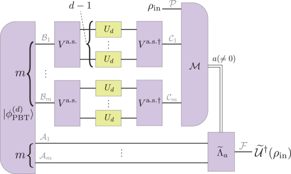
Figure 11: A quantum circuit representation of a parallel protocol for unitary inversion from k=m(d1)k=m(d-1) calls of Ud𝕌(d)U_{d}\in\mathbb{U}(d) [18]. Each wire corresponds to a dd-dimensional system. The quantum state |ϕPBT(d)|{\phi^{(d)}_{\mathrm{PBT}}}\rangle and the POVM ={Γa(d)}a=0k\mathcal{M}=\{\Gamma_{a}^{(d)}\}_{a=0}^{k} are the optimal resource state and the POVM for the probabilistic port-based teleportation [67, 68], which are defined in Eqs. (100) and (101), respectively. The isometry operator Va.s.V^{\mathrm{a.s.}} represents an encoding of quantum information on a totally antisymmetric state defined in Eq. (62). The conditional CPTP map Λ~a\widetilde{\Lambda}_{a} is the operation to select the quantum state in 𝒜a\mathcal{A}_{a} corresponding to the measurement outcome aa of \mathcal{M} as the output state for a0a\neq 0, which is defined in Eq. (111). This protocol succeeds when the measurement outcome aa is a0a\neq 0.

We show a quantum circuit representation of a kk-input unitary inversion protocol presented in Ref. [18] (See Figure 11). This protocol achieves a success probability psucc=k/(d1)/[d2+k/(d1)1]p_{\mathrm{succ}}=\lfloor k/(d-1)\rfloor/[d^{2}+\lfloor k/(d-1)\rfloor-1]. In Figure 11, each wire corresponds to a dd-dimensional system. We define the joint Hilbert spaces by 𝒜i=1m𝒜i\mathcal{A}\coloneqq\bigotimes_{i=1}^{m}\mathcal{A}_{i}, i=1mi\mathcal{B}\coloneqq\bigotimes_{i=1}^{m}\mathcal{B}_{i}, 𝒞i=1m𝒞i\mathcal{C}\coloneqq\bigotimes_{i=1}^{m}\mathcal{C}_{i} and 𝒞¯aia𝒞i\overline{\mathcal{C}}_{a}\coloneqq\bigotimes_{i\neq a}\mathcal{C}_{i} for a{1,,m}a\in\{1,\cdots,m\}. The quantum state |ϕPBT(d)𝒜|{\phi^{(d)}_{\mathrm{PBT}}}\rangle\in\mathcal{A}\otimes\mathcal{B} and the POVM ={Γa(d)}a=0k\mathcal{M}=\{\Gamma_{a}^{(d)}\}_{a=0}^{k} are the optimal resource state and the POVM for the probabilistic port-based teleportation [67, 68], respectively, which are defined by

|ϕPBT(d)(X12𝟙𝒜)|Φdk+𝒜,\displaystyle|{\phi^{(d)}_{\mathrm{PBT}}}\rangle\coloneqq(X^{\prime\frac{1}{2}}_{\mathcal{B}}\otimes\mathds{1}_{\mathcal{A}})|{\Phi^{+}_{d^{k}}}\rangle_{\mathcal{BA}}, (100)
Γa(d)(𝟙𝒫X𝒞12)(|Φd+Φd+|𝒫𝒞aΘ𝒞¯a)(𝟙𝒫X𝒞12),\displaystyle\Gamma^{(d)}_{a}\coloneqq(\mathds{1}_{\mathcal{P}}\otimes X^{\prime-\frac{1}{2}}_{\mathcal{C}})\left(|{\Phi^{+}_{d}}\rangle\!\langle{\Phi^{+}_{d}}|_{\mathcal{P}\mathcal{C}_{a}}\otimes\Theta^{\prime}_{\overline{\mathcal{C}}_{a}}\right)(\mathds{1}_{\mathcal{P}}\otimes X^{\prime-\frac{1}{2}}_{\mathcal{C}}), (101)

where Θ𝒞¯a\Theta^{\prime}_{\overline{\mathcal{C}}_{a}} and XX^{\prime}_{\mathcal{B}} are defined similarly to Eqs. (107) and (108) as

Θ𝒞¯a\displaystyle\Theta^{\prime}_{\overline{\mathcal{C}}_{a}} αm1dm+1gd(m)d𝒰α(d)md𝒮α(m1)Πα,𝒞¯a,\displaystyle\coloneqq\sum_{\alpha\vdash m-1}\frac{d^{m+1}g_{d}(m)d_{\mathcal{U}^{(d)}_{\alpha}}}{md_{\mathcal{S}^{(m-1)}_{\alpha}}}\Pi_{\alpha,\overline{\mathcal{C}}_{a}}, (102)
X\displaystyle X^{\prime}_{\mathcal{B}} μmdmgd(m)d𝒰μ(d)d𝒮μ(m)Πμ,,\displaystyle\coloneqq\sum_{\mu\vdash m}\frac{d^{m}g_{d}(m)d_{\mathcal{U}^{(d)}_{\mu}}}{d_{\mathcal{S}^{(m)}_{\mu}}}\Pi_{\mu,\mathcal{B}}, (103)

and |Φdk+|{\Phi^{+}_{d^{k}}}\rangle and |Φd+|{\Phi^{+}_{d}}\rangle are the maximally entangled states defined in Eqs. (106) and (66). The conditional CPTP map Λ~a\widetilde{\Lambda}_{a} and the isometry operator Va.s.V^{\mathrm{a.s.}} are defined in Eqs. (111) and (62), respectively.

Appendix E Parallel isometry transposition

E.1 Construction of parallel isometry transposition protocol

We can construct a parallel protocol for isometry transposition similarly to unitary transposition [19] based on the port-based teleportation [67, 68] and obtain the success probability of the protocol as stated in the following Theorem.

Theorem 8.

A parallel protocol shown in Figure 12 transforms kk calls of an isometry operation 𝒱~\widetilde{\mathcal{V}} corresponding to V𝕍iso(d,D)V\in\mathbb{V}_{\mathrm{iso}}(d,D) into its transposed map 𝒱~T\widetilde{\mathcal{V}}^{T} with a success probability psucc=k/(Dd+k1)p_{\mathrm{succ}}=k/(Dd+k-1).

Figure 12: A quantum circuit representation of a probabilistic parallel protocol for isometry transposition. The quantum state |ϕPBT|{\phi_{\mathrm{PBT}}^{\prime}}\rangle is a modified state of the optimal resource state for the probabilistic port-based teleportation [67, 68] defined in Eq. (105). The POVM ={Γa(D)}a=0k\mathcal{M}=\{\Gamma^{(D)}_{a}\}_{a=0}^{k} is also the optimal POVM for the probabilistic port-based teleportation, which is defined in Eq. (110). The conditional CPTP map Λ~a\widetilde{\Lambda}_{a} is the operation to select the quantum state in 𝒜a\mathcal{A}_{a} corresponding to the measurement outcome aa of \mathcal{M} as the output state for a0a\neq 0, which is defined in Eq. (111). This protocol succeeds when the measurement outcome aa is a0a\neq 0.

In Figure 12, the Hilbert spaces are given by =d\mathcal{F}=\mathbb{C}^{d}, i=d\mathcal{I}_{i}=\mathbb{C}^{d}, 𝒜i=d\mathcal{A}_{i}=\mathbb{C}^{d}, 𝒫=D\mathcal{P}=\mathbb{C}^{D}, and 𝒪i=D\mathcal{O}_{i}=\mathbb{C}^{D} for i{1,,k}i\in\{1,\cdots,k\}. We define the joint Hilbert spaces by i=1ki\mathcal{I}\coloneqq\bigotimes_{i=1}^{k}\mathcal{I}_{i}, 𝒪i=1k𝒪i\mathcal{O}\coloneqq\bigotimes_{i=1}^{k}\mathcal{O}_{i}, 𝒪¯aia𝒪i\overline{\mathcal{O}}_{a}\coloneqq\bigotimes_{i\neq a}\mathcal{O}_{i} and 𝒜i=1k𝒜i\mathcal{A}\coloneqq\bigotimes_{i=1}^{k}\mathcal{A}_{i}. The quantum state |ϕPBT|{\phi_{\mathrm{PBT}}^{\prime}}\rangle, the POVM \mathcal{M}, and the conditional CPTP map Λ~a\widetilde{\Lambda}_{a} are defined as follows.

To define |ϕPBT𝒜|{\phi^{\prime}_{\mathrm{PBT}}}\rangle\in\mathcal{I}\otimes\mathcal{A}, we firstly define an operator YY_{\mathcal{I}} by

Y1μkd𝒰μ(d)d𝒰μ(D)μkdkd𝒰μ(D)d𝒮μ(k)Πμ,,\displaystyle Y_{\mathcal{I}}\coloneqq\frac{1}{\sum_{\mu\vdash k}d_{\mathcal{U}^{(d)}_{\mu}}d_{\mathcal{U}^{(D)}_{\mu}}}\sum_{\mu\vdash k}\frac{d^{k}d_{\mathcal{U}^{(D)}_{\mu}}}{d_{\mathcal{S}_{\mu}^{(k)}}}\Pi_{\mu,\mathcal{I}}, (104)

where d𝒰μ(d)d_{\mathcal{U}^{(d^{\prime})}_{\mu}} and d𝒮μ(k)d_{\mathcal{S}_{\mu}^{(k)}} are the dimensions of 𝒰μ,dk(D)\mathcal{U}^{(D)}_{\mu,\mathbb{C}^{d^{\prime}\otimes k}} and 𝒮μ,Dk(k)\mathcal{S}^{(k)}_{\mu,\mathbb{C}^{D\otimes{k}}} for d{d,D}d^{\prime}\in\{d,D\}, respectively, and Πμ,\Pi_{\mu,\mathcal{I}} is the orthogonal projector on \mathcal{I} onto its subspace 𝒰μ,(d)𝒮μ,(k)\mathcal{U}^{({d^{\prime}})}_{\mu,\mathcal{I}}\otimes\mathcal{S}^{(k)}_{\mu,\mathcal{I}}. Then, we define |ϕPBT𝒜|{\phi^{\prime}_{\mathrm{PBT}}}\rangle\in\mathcal{I}\otimes\mathcal{A} by

|ϕPBT\displaystyle|{\phi^{\prime}_{\mathrm{PBT}}}\rangle\coloneqq (Y12I𝒜)|Φdk+𝒜,\displaystyle(Y^{\frac{1}{2}}_{\mathcal{I}}\otimes I_{\mathcal{A}})|{\Phi^{+}_{d^{k}}}\rangle_{\mathcal{IA}}, (105)

where |Φdk+𝒜|{\Phi^{+}_{d^{k}}}\rangle_{\mathcal{IA}} is the maximally entangled state given by

|Φdk+𝒜1dki=0dk1|i|i𝒜\displaystyle|{\Phi^{+}_{d^{k}}}\rangle_{\mathcal{IA}}\coloneqq\frac{1}{\sqrt{d^{k}}}\sum_{i=0}^{d^{k}-1}|{i}\rangle\otimes|{i}\rangle\in\mathcal{I}\otimes\mathcal{A} (106)

in terms of the computational basis {|i}\{|{i}\rangle\} of \mathcal{I} and 𝒜\mathcal{A}. The state |ϕPBT|{\phi^{\prime}_{\mathrm{PBT}}}\rangle is a modified state of the optimal resource state |ϕPBT(d)|{\phi^{(d)}_{\mathrm{PBT}}}\rangle for the probabilistic port-based teleportation of a dd-dimensional quantum state [67, 68] (see Appendix D for the definition of |ϕPBT(d)|{\phi^{(d)}_{\mathrm{PBT}}}\rangle).

The POVM ={Γa(D)}a=0k\mathcal{M}=\{\Gamma^{(D)}_{a}\}_{a=0}^{k} is defined as follows. We define operators Θ𝒪¯a\Theta_{\overline{\mathcal{O}}_{a}} and X𝒪X_{\mathcal{O}} by

Θ𝒪¯a\displaystyle\Theta_{\overline{\mathcal{O}}_{a}} αk1Dk+1gD(k)d𝒰α(D)kd𝒮α(k1)Πα,𝒪¯a,\displaystyle\coloneqq\sum_{\alpha\vdash k-1}\frac{D^{k+1}g_{D}(k)d_{\mathcal{U}^{(D)}_{\alpha}}}{kd_{\mathcal{S}^{(k-1)}_{\alpha}}}\Pi_{\alpha,\overline{\mathcal{O}}_{a}}, (107)
X𝒪\displaystyle X_{\mathcal{O}} μkDkgD(k)d𝒰μ(D)d𝒮μ(k)Πμ,𝒪,\displaystyle\coloneqq\sum_{\mu\vdash k}\frac{D^{k}g_{D}(k)d_{\mathcal{U}^{(D)}_{\mu}}}{d_{\mathcal{S}^{(k)}_{\mu}}}\Pi_{\mu,\mathcal{O}}, (108)

where d𝒰α(D)d_{\mathcal{U}^{(D)}_{\alpha}} and dSα(k1)d_{S^{(k-1)}_{\alpha}} are defined similarly to d𝒰μ(D)d_{\mathcal{U}^{(D)}_{\mu}} and d𝒮μ(k)d_{\mathcal{S}_{\mu}^{(k)}}, respectively, gD(k)g_{D}(k) is defined by

gD(k)[μk(d𝒰μ(D))2]1\displaystyle g_{D}(k)\coloneqq\left[\sum_{\mu\vdash k}\left(d_{\mathcal{U}^{(D)}_{\mu}}\right)^{2}\right]^{-1} (109)

and Πα,𝒪¯a\Pi_{\alpha,\overline{\mathcal{O}}_{a}} and Πμ,𝒪\Pi_{\mu,\mathcal{O}} are orthogonal projectors defined similarly to Πμ,\Pi_{\mu,\mathcal{I}}. Using Θ𝒪¯a\Theta_{\overline{\mathcal{O}}_{a}} and X𝒪X_{\mathcal{O}}, we define an operator Γa(D)(a{1,,k})\Gamma^{(D)}_{a}\;(a\in\{1,\cdots,k\}) on 𝒫𝒪\mathcal{P}\otimes\mathcal{O} by

Γa(D)\displaystyle\Gamma^{(D)}_{a} (𝟙𝒫X𝒪12)(|ΦD+ΦD+|𝒫𝒪aΘ𝒪¯a)(𝟙𝒫X𝒪12).\displaystyle\coloneqq(\mathds{1}_{\mathcal{P}}\otimes X_{\mathcal{O}}^{-\frac{1}{2}})\left(|{\Phi^{+}_{D}}\rangle\!\langle{\Phi^{+}_{D}}|_{\mathcal{P}\mathcal{O}_{a}}\otimes\Theta_{\overline{\mathcal{O}}_{a}}\right)(\mathds{1}_{\mathcal{P}}\otimes X_{\mathcal{O}}^{-\frac{1}{2}}). (110)

The set of operators {Γa(D)}a=1k\{\Gamma^{(D)}_{a}\}_{a=1}^{k} satisfies Γa(D)0\Gamma^{(D)}_{a}\geq 0 for a{1,,k}a\in\{1,\cdots,k\} and a=1kΓa(D)𝟙𝒫𝒪\sum_{a=1}^{k}\Gamma^{(D)}_{a}\leq\mathds{1}_{\mathcal{P}\mathcal{O}} [68]. Thus, by defining Γ0(D)𝟙𝒫𝒪a=1kΓa(D)\Gamma^{(D)}_{0}\coloneqq\mathds{1}_{\mathcal{PO}}-\sum_{a=1}^{k}\Gamma^{(D)}_{a}, a set of operators {Γa(D)}a=0k\{\Gamma^{(D)}_{a}\}_{a=0}^{k} forms a POVM. The POVM {Γa(D)}a=0k\{\Gamma^{(D)}_{a}\}_{a=0}^{k} is the optimal POVM for the probabilistic port-based teleportation of a DD-dimensional quantum state [67, 68].

The conditional CPTP map Λ~a:(𝒜)()\widetilde{\Lambda}_{a}:\mathcal{L}(\mathcal{A})\to\mathcal{L}(\mathcal{F}) for the outcome a{1,,k}a\in\{1,\cdots,k\} of \mathcal{M} is defined by

Λ~a(ρ𝒜)=j,j|jj|j|Tr𝒜¯aρ𝒜|j,\displaystyle\widetilde{\Lambda}_{a}(\rho_{\mathcal{A}})=\sum_{j,j^{\prime}}|{j}\rangle\!\langle{j^{\prime}}|_{\mathcal{F}}\langle{j}|{\mathrm{Tr}}_{\overline{\mathcal{A}}_{a}}\rho_{\mathcal{A}}|{j^{\prime}}\rangle, (111)

where {|j}\{|{j}\rangle\} is the computational basis of Hilbert spaces 𝒜a\mathcal{A}_{a} and \mathcal{F}. This conditional CPTP map represents the operation to select the quantum state in 𝒜a\mathcal{A}_{a} corresponding to the measurement outcome aa as the output state. The conditional CPTP map corresponding to the measurement outcome a=0a=0 is not needed since our protocol only succeeds for a0a\neq 0 and the output state is aborted if a=0a=0, the failure case.

The protocol presented above is shown to implement isometry transposition with the success probability psucc=k/(Dd+k1)p_{\text{succ}}=k/(Dd+k-1).

Proof of Theorem 8.

First, we show the equality

(V𝒪k𝟙𝒜)|ϕPBT𝒜=μk(d𝒰μ(D))2μkd𝒰μ(d)d𝒰μ(D)(𝟙𝒪V𝒜Tk)|ϕPBT(D)𝒪,\displaystyle(V^{\otimes k}_{\mathcal{I}\to\mathcal{O}}\otimes\mathds{1}_{\mathcal{A}})|{\phi^{\prime}_{\mathrm{PBT}}}\rangle_{\mathcal{I}\mathcal{A}}=\sqrt{\frac{\sum_{\mu\vdash k}(d_{\mathcal{U}^{(D)}_{\mu}})^{2}}{\sum_{\mu\vdash k}d_{\mathcal{U}^{(d)}_{\mu}}d_{\mathcal{U}^{(D)}_{\mu}}}}(\mathds{1}_{\mathcal{O}}\otimes V^{T\otimes k}_{\mathcal{B}\to\mathcal{A}})|{\phi^{(D)}_{\mathrm{PBT}}}\rangle_{\mathcal{O}\mathcal{B}}, (112)

where the joint Hilbert space \mathcal{B} is defined by i=1ki\mathcal{B}\coloneqq\bigotimes_{i=1}^{k}\mathcal{B}_{i} for i=D\mathcal{B}_{i}=\mathbb{C}^{D}, and the quantum state |ϕPBT(D)𝒪|{\phi^{(D)}_{\mathrm{PBT}}}\rangle\in\mathcal{O}\otimes\mathcal{B} is the optimal resource state for the probabilistic port-based teleportation of a DD-dimensional quantum state [67, 68] defined by

|ϕPBT(D)(X𝒪12𝟙)|ΦDk+𝒪\displaystyle|{\phi^{(D)}_{\mathrm{PBT}}}\rangle\coloneqq(X_{\mathcal{O}}^{\frac{1}{2}}\otimes\mathds{1}_{\mathcal{B}})|{\Phi^{+}_{D^{k}}}\rangle_{\mathcal{OB}} (113)

using X𝒪X_{\mathcal{O}} given in Eq. (108) and the maximally entangled state |ΦDk+|{\Phi^{+}_{D^{k}}}\rangle. To show this equality, we define the maximally entangled state for each μ\mu denoted as |ϕd,μ+(𝒰μ,(d)𝒮μ,(k))(𝒰μ,𝒜(d)𝒮μ,𝒜(k))|{\phi^{+}_{d,\mu}}\rangle\in(\mathcal{U}^{(d)}_{\mu,\mathcal{I}}\otimes\mathcal{S}^{(k)}_{\mu,\mathcal{I}})\otimes(\mathcal{U}^{(d)}_{\mu,\mathcal{A}}\otimes\mathcal{S}^{(k)}_{\mu,\mathcal{A}}) given by

|ϕd,μ+𝒜1d𝒰μ(d)d𝒮μ(k)uμ,sμ|μ,uμ,sμ|μ,uμ,sμ𝒜,\displaystyle|{\phi^{+}_{d,\mu}}\rangle_{\mathcal{IA}}\coloneqq\frac{1}{\sqrt{d_{\mathcal{U}^{(d)}_{\mu}}d_{\mathcal{S}^{(k)}_{\mu}}}}\sum_{u_{\mu},s_{\mu}}|{\mu,u_{\mu},s_{\mu}}\rangle_{\mathcal{I}}\otimes|{\mu,u_{\mu},s_{\mu}}\rangle_{\mathcal{A}}, (114)

where {|μ,uμ,sμ}\{|{\mu,u_{\mu},s_{\mu}}\rangle\} is the Schur basis. Similarly, we define the maximally entangled state for each μ\mu denoted as |ϕD,μ+(𝒰μ,𝒪(D)𝒮μ,𝒪(k))(𝒰μ,(D)𝒮μ,(k))|{\phi^{+}_{D,\mu}}\rangle\in(\mathcal{U}^{(D)}_{\mu,\mathcal{O}}\otimes\mathcal{S}^{(k)}_{\mu,\mathcal{O}})\otimes(\mathcal{U}^{(D)}_{\mu,\mathcal{B}}\otimes\mathcal{S}^{(k)}_{\mu,\mathcal{B}}). Then, the quantum state |ϕPBT|{\phi^{\prime}_{\mathrm{PBT}}}\rangle defined in Eq. (105) can be written as

|ϕPBT\displaystyle|{\phi^{\prime}_{\mathrm{PBT}}}\rangle
=μkdkd𝒰μ(D)d𝒮μ(k)νkd𝒰ν(d)d𝒰ν(D)(Πμ,𝟙𝒜)|Φdk+𝒜\displaystyle=\sum_{\mu\vdash k}\sqrt{\frac{d^{k}d_{\mathcal{U}^{(D)}_{\mu}}}{d_{\mathcal{S}^{(k)}_{\mu}}\sum_{\nu\vdash k}d_{\mathcal{U}^{(d)}_{\nu}}d_{\mathcal{U}^{(D)}_{\nu}}}}(\Pi_{\mu,\mathcal{I}}\otimes\mathds{1}_{\mathcal{A}})|{\Phi^{+}_{d^{k}}}\rangle_{\mathcal{IA}} (115)
=μkdkd𝒰μ(D)d𝒮μ(k)νkd𝒰ν(d)d𝒰ν(D)(Πμ,𝟙𝒜)νkd𝒰ν(d)d𝒮ν(k)dk(USchU𝒜Sch)|ϕd,ν+𝒜\displaystyle=\sum_{\mu\vdash k}\sqrt{\frac{d^{k}d_{\mathcal{U}^{(D)}_{\mu}}}{d_{\mathcal{S}^{(k)}_{\mu}}\sum_{\nu\vdash k}d_{\mathcal{U}^{(d)}_{\nu}}d_{\mathcal{U}^{(D)}_{\nu}}}}(\Pi_{\mu,\mathcal{I}}\otimes\mathds{1}_{\mathcal{A}})\sum_{\nu\vdash k}\sqrt{\frac{d_{\mathcal{U}_{\nu}^{(d)}}d_{\mathcal{S}_{\nu}^{(k)}}}{d^{k}}}(U^{\mathrm{Sch}\dagger}_{\mathcal{I}}\otimes U^{\mathrm{Sch}\dagger}_{\mathcal{A}})|{\phi^{+}_{d,\nu}}\rangle_{\mathcal{IA}} (116)
=μkpμ[𝟙U𝒜Sch(U𝒜Sch)t]|ϕd,μ+𝒜,\displaystyle=\sum_{\mu\vdash k}p_{\mu}[\mathds{1}_{\mathcal{I}}\otimes{U^{\mathrm{Sch}\dagger}_{\mathcal{A}}(U^{\mathrm{Sch}\dagger}_{\mathcal{A}})^{t}}]|{\phi^{+}_{d,\mu}}\rangle_{\mathcal{IA}}, (117)

where USchU^{\mathrm{Sch}} is the quantum Schur transforms defined above Lemma 4, pμp_{\mu} is a positive value given by

pμd𝒰μ(d)d𝒰μ(D)νkd𝒰ν(d)d𝒰ν(D),\displaystyle p_{\mu}\coloneqq\sqrt{\frac{d_{\mathcal{U}_{\mu}^{(d)}}d_{\mathcal{U}_{\mu}^{(D)}}}{\sum_{\nu\vdash k}d_{\mathcal{U}_{\nu}^{(d)}}d_{\mathcal{U}_{\nu}^{(D)}}}}, (118)

and XtX^{t} denotes the transpose of XX in the Schur basis. Similarly, |ϕPBT(D)|{\phi^{(D)}_{\mathrm{PBT}}}\rangle is calculated as

|ϕPBT(D)𝒪=μkqμ[𝟙USch(USch)t]|ϕD,μ+𝒪,\displaystyle|{\phi^{(D)}_{\mathrm{PBT}}}\rangle_{\mathcal{OB}}=\sum_{\mu\vdash k}q_{\mu}[\mathds{1}_{\mathcal{I}}\otimes{U^{\mathrm{Sch}\dagger}_{\mathcal{B}}(U^{\mathrm{Sch}\dagger}_{\mathcal{B}})^{t}}]|{\phi^{+}_{D,\mu}}\rangle_{\mathcal{OB}}, (119)

where qμq_{\mu} is a positive value given by

qμd𝒰μ(D)νk(d𝒰ν(D))2.\displaystyle q_{\mu}\coloneqq\frac{d_{\mathcal{U}^{(D)}_{\mu}}}{\sqrt{\sum_{\nu\vdash k}(d_{\mathcal{U}^{(D)}_{\nu}})^{2}}}. (120)

Since a tensor product VkV^{\otimes k} of an isometry operator V𝕍iso(d,D)V\in\mathbb{V}_{\mathrm{iso}}(d,D) can be decomposed in the irreducible representation form as Eq. (89), we obtain

(V𝒪k𝟙𝒜)|ϕPBT𝒜\displaystyle(V^{\otimes k}_{\mathcal{I}\to\mathcal{O}}\otimes\mathds{1}_{\mathcal{A}})|{\phi^{\prime}_{\mathrm{PBT}}}\rangle_{\mathcal{IA}} =μpμ(V𝒪k𝟙𝒜)[𝟙U𝒜Sch(U𝒜Sch)t]|ϕd,μ+𝒜\displaystyle=\sum_{\mu}p_{\mu}(V^{\otimes k}_{\mathcal{I}\to\mathcal{O}}\otimes\mathds{1}_{\mathcal{A}})[\mathds{1}_{\mathcal{I}}\otimes{U^{\mathrm{Sch}\dagger}_{\mathcal{A}}(U^{\mathrm{Sch}\dagger}_{\mathcal{A}})^{t}}]|{\phi^{+}_{d,\mu}}\rangle_{\mathcal{IA}} (121)
=μpμ[VμI𝒮μ,(k)𝒮μ,𝒪(k)U𝒜Sch(U𝒜Sch)t]|ϕd,μ+𝒜\displaystyle=\sum_{\mu}p_{\mu}\left[V_{\mu}\otimes I_{\mathcal{S}^{(k)}_{\mu,\mathcal{I}}\to\mathcal{S}^{(k)}_{\mu,\mathcal{O}}}\otimes{U^{\mathrm{Sch}\dagger}_{\mathcal{A}}(U^{\mathrm{Sch}\dagger}_{\mathcal{A}})^{t}}\right]|{\phi^{+}_{d,\mu}}\rangle_{\mathcal{IA}} (122)
=μrμ[𝟙𝒪U𝒜Sch(U𝒜Sch)t](VμI𝒮μ,𝒜(k)𝒮μ,(k))t|ϕD,μ+𝒪,\displaystyle=\sum_{\mu}r_{\mu}[\mathds{1}_{\mathcal{O}}\otimes{U^{\mathrm{Sch}\dagger}_{\mathcal{A}}(U^{\mathrm{Sch}\dagger}_{\mathcal{A}})^{t}}]\left(V_{\mu}\otimes I_{\mathcal{S}^{(k)}_{\mu,\mathcal{A}}\to\mathcal{S}^{(k)}_{\mu,\mathcal{B}}}\right)^{t}|{\phi^{+}_{D,\mu}}\rangle_{\mathcal{OB}}, (123)

where rμr_{\mu} is a positive value given by

rμpμd𝒰μ(D)d𝒰μ(d)=d𝒰μ(D)νkd𝒰ν(d)d𝒰ν(D).\displaystyle r_{\mu}\coloneqq p_{\mu}\sqrt{\frac{d_{\mathcal{U}^{(D)}_{\mu}}}{d_{\mathcal{U}^{(d)}_{\mu}}}}=\frac{d_{\mathcal{U}^{(D)}_{\mu}}}{\sqrt{\sum_{\nu\vdash k}d_{\mathcal{U}^{(d)}_{\nu}}d_{\mathcal{U}^{(D)}_{\nu}}}}. (124)

For X:𝒜X:\mathcal{A}\to\mathcal{B}, the transpose XtX^{t} in the Schur basis can be converted to the transpose XTX^{T} in the computational basis as

XT\displaystyle X^{T} =U𝒜Sch(USchX𝒜U𝒜Sch)tUSch\displaystyle={U^{\mathrm{Sch}\dagger}_{\mathcal{A}}(U^{\mathrm{Sch}}_{\mathcal{B}}}X_{\mathcal{A}\to\mathcal{B}}{U^{\mathrm{Sch}\dagger}_{\mathcal{A}})^{t}U^{\mathrm{Sch}}_{\mathcal{B}}} (125)
=U𝒜Sch(U𝒜Sch)tX𝒜t(USch)tUSch.\displaystyle={U^{\mathrm{Sch}\dagger}_{\mathcal{A}}(U^{\mathrm{Sch}\dagger}_{\mathcal{A}})^{t}}X^{t}_{\mathcal{B}\to\mathcal{A}}{(U^{\mathrm{Sch}}_{\mathcal{B}})^{t}U^{\mathrm{Sch}}_{\mathcal{B}}}. (126)

Using this relation, we proceed the calculation in Eq. (123) as

(V𝒪k𝟙𝒜)|ϕPBT𝒜\displaystyle(V^{\otimes k}_{\mathcal{I}\to\mathcal{O}}\otimes\mathds{1}_{\mathcal{A}})|{\phi^{\prime}_{\mathrm{PBT}}}\rangle_{\mathcal{IA}} =μrμ{𝟙𝒪[(VμI𝒮μ,𝒜(k)𝒮μ,(k))TUSch(USch)t]}|ϕD,μ+𝒪.\displaystyle=\sum_{\mu}r_{\mu}\left\{\mathds{1}_{\mathcal{O}}\otimes\left[\left(V_{\mu}\otimes I_{\mathcal{S}^{(k)}_{\mu,\mathcal{A}}\to\mathcal{S}^{(k)}_{\mu,\mathcal{B}}}\right)^{T}{U^{\mathrm{Sch}\dagger}_{\mathcal{B}}(U^{\mathrm{Sch}\dagger}_{\mathcal{B}})^{t}}\right]\right\}|{\phi^{+}_{D,\mu}}\rangle_{\mathcal{OB}}. (127)

From Eqs. (119), (120), (124) and (127), we obtain Eq. (112).

Let ρout,a(𝒜a)\rho^{\prime}_{\mathrm{out},a}\in\mathcal{L}(\mathcal{A}_{a}) be the output state after obtaining the outcome aa of the POVM ={Γa(D)}\mathcal{M}=\{\Gamma^{(D)}_{a}\} given by Eq. (110), but before applying the correction Λ~a\widetilde{\Lambda}_{a} given by Eq. (111). For a0a\neq 0, the output state ρout,a\rho^{\prime}_{\mathrm{out},a} multiplied by the probability to obtain the measurement outcome aa, denoted by ρout,a\rho_{\mathrm{out},a}, is calculated as

ρout,a\displaystyle\rho_{\mathrm{out},a}
=Tr𝒫𝒪𝒜¯a((Γa,𝒫𝒪𝟙𝒜){ρin,𝒫[𝒱~𝒪k𝟙~𝒜(|ϕPBTϕPBT|𝒜)]})\displaystyle={\mathrm{Tr}}_{\mathcal{P}\mathcal{O}\overline{\mathcal{A}}_{a}}\left((\Gamma_{a,\mathcal{PO}}\otimes\mathds{1}_{\mathcal{A}})\left\{\rho_{\mathrm{in},\mathcal{P}}\otimes\left[\widetilde{\mathcal{V}}^{\otimes k}_{\mathcal{I}\to\mathcal{O}}\otimes\widetilde{\mathds{1}}_{\mathcal{A}}(|{\phi^{\prime}_{\mathrm{PBT}}}\rangle\!\langle{\phi^{\prime}_{\mathrm{PBT}}}|_{\mathcal{IA}})\right]\right\}\right) (128)
=μk(d𝒰μ(D))2μkd𝒰μ(d)d𝒰μ(D)Tr𝒫𝒪𝒜¯a((Γa,𝒫𝒪𝟙𝒜){ρin,𝒫[𝟙~𝒪𝒱~𝒜Tk(|ϕPBTϕPBT|𝒪)]})\displaystyle=\frac{\sum_{\mu\vdash k}(d_{\mathcal{U}^{(D)}_{\mu}})^{2}}{\sum_{\mu\vdash k}d_{\mathcal{U}^{(d)}_{\mu}}d_{\mathcal{U}^{(D)}_{\mu}}}{\mathrm{Tr}}_{\mathcal{P}\mathcal{O}\overline{\mathcal{A}}_{a}}\left((\Gamma_{a,\mathcal{PO}}\otimes\mathds{1}_{\mathcal{A}})\left\{\rho_{\mathrm{in},\mathcal{P}}\otimes\left[\widetilde{\mathds{1}}_{\mathcal{O}}\otimes\widetilde{\mathcal{V}}^{T\otimes k}_{\mathcal{B}\to\mathcal{A}}(|{\phi_{\mathrm{PBT}}}\rangle\!\langle{\phi_{\mathrm{PBT}}}|_{\mathcal{OB}})\right]\right\}\right) (129)
=μk(d𝒰μ(D))2μkd𝒰μ(d)d𝒰μ(D)Tr𝒫𝒪𝒜¯a((Γa,𝒫𝒪𝟙𝒜){ρin,𝒫[𝒳~𝒪12𝒱~𝒜Tk(|ΦDk+ΦDk+|𝒪)]})\displaystyle=\frac{\sum_{\mu\vdash k}(d_{\mathcal{U}^{(D)}_{\mu}})^{2}}{\sum_{\mu\vdash k}d_{\mathcal{U}^{(d)}_{\mu}}d_{\mathcal{U}^{(D)}_{\mu}}}{\mathrm{Tr}}_{\mathcal{P}\mathcal{O}\overline{\mathcal{A}}_{a}}\left((\Gamma_{a,\mathcal{PO}}\otimes\mathds{1}_{\mathcal{A}})\left\{\rho_{\mathrm{in},\mathcal{P}}\otimes\left[\widetilde{\mathcal{X}}^{\frac{1}{2}}_{\mathcal{O}}\otimes\widetilde{\mathcal{V}}^{T\otimes k}_{\mathcal{B}\to\mathcal{A}}(|{\Phi^{+}_{D^{k}}}\rangle\!\langle{\Phi^{+}_{D^{k}}}|_{\mathcal{OB}})\right]\right\}\right) (130)
=μk(d𝒰μ(D))2μkd𝒰μ(d)d𝒰μ(D)\displaystyle=\frac{\sum_{\mu\vdash k}(d_{\mathcal{U}^{(D)}_{\mu}})^{2}}{\sum_{\mu\vdash k}d_{\mathcal{U}^{(d)}_{\mu}}d_{\mathcal{U}^{(D)}_{\mu}}}
×Tr𝒫𝒪𝒜¯a([𝟙~𝒫𝒳~𝒪12(Γa,𝒫𝒪)𝟙𝒜]{ρin,𝒫[𝟙~𝒪𝒱~𝒜Tk(|ΦDk+ΦDk+|𝒪)]}).\displaystyle\hskip 12.0pt\times{\mathrm{Tr}}_{\mathcal{P}\mathcal{O}\overline{\mathcal{A}}_{a}}\left(\left[\widetilde{\mathds{1}}_{\mathcal{P}}\otimes\widetilde{\mathcal{X}}^{\dagger\frac{1}{2}}_{\mathcal{O}}(\Gamma_{a,\mathcal{PO}})\otimes\mathds{1}_{\mathcal{A}}\right]\left\{\rho_{\mathrm{in},\mathcal{P}}\otimes\left[\widetilde{\mathds{1}}_{\mathcal{O}}\otimes\widetilde{\mathcal{V}}^{T\otimes k}_{\mathcal{B}\to\mathcal{A}}(|{\Phi^{+}_{D^{k}}}\rangle\!\langle{\Phi^{+}_{D^{k}}}|_{\mathcal{OB}})\right]\right\}\right). (131)

Since X𝒪=X𝒪X_{\mathcal{O}}=X_{\mathcal{O}}^{\dagger} holds and the definition of Γa\Gamma_{a} is given by Eq. (110), we obtain

(𝟙~𝒫𝒳~𝒪12)(Γa,𝒫𝒪)=|ΦD+ΦD+|𝒫𝒪aΘ𝒪¯a.\displaystyle\left(\widetilde{\mathds{1}}_{\mathcal{P}}\otimes\widetilde{\mathcal{X}}^{\dagger\frac{1}{2}}_{\mathcal{O}}\right)(\Gamma_{a,\mathcal{PO}})=|{\Phi^{+}_{D}}\rangle\!\langle{\Phi^{+}_{D}}|_{\mathcal{P}\mathcal{O}_{a}}\otimes\Theta_{\overline{\mathcal{O}}_{a}}. (132)

Therefore, ρout,a\rho_{\mathrm{out},a} is further calculated as

ρout,a\displaystyle\rho_{\mathrm{out},a}
=μk(d𝒰μ(D))2μkd𝒰μ(d)d𝒰μ(D)\displaystyle=\frac{\sum_{\mu\vdash k}(d_{\mathcal{U}^{(D)}_{\mu}})^{2}}{\sum_{\mu\vdash k}d_{\mathcal{U}^{(d)}_{\mu}}d_{\mathcal{U}^{(D)}_{\mu}}}
×Tr𝒫𝒪𝒜¯a((|ΦD+ΦD+|𝒫𝒪aΘ𝒪¯a𝟙𝒜){ρin,𝒫[𝟙~𝒪𝒱~𝒜Tk(|ΦDk+ΦDk+|𝒪)]})\displaystyle\hskip 12.0pt\times{\mathrm{Tr}}_{\mathcal{P}\mathcal{O}\overline{\mathcal{A}}_{a}}\left((|{\Phi^{+}_{D}}\rangle\!\langle{\Phi^{+}_{D}}|_{\mathcal{P}\mathcal{O}_{a}}\otimes\Theta_{\overline{\mathcal{O}}_{a}}\otimes\mathds{1}_{\mathcal{A}})\left\{\rho_{\mathrm{in},\mathcal{P}}\otimes\left[\widetilde{\mathds{1}}_{\mathcal{O}}\otimes\widetilde{\mathcal{V}}^{T\otimes k}_{\mathcal{B}\to\mathcal{A}}(|{\Phi^{+}_{D^{k}}}\rangle\!\langle{\Phi^{+}_{D^{k}}}|_{\mathcal{OB}})\right]\right\}\right) (133)
=μk(d𝒰μ(D))2μkd𝒰μ(d)d𝒰μ(D)Tr{(Θ𝒪¯a𝟙𝒜¯a)[𝟙~𝒪¯a𝒱~¯a𝒜¯aTk1(|ΦDk1+ΦDk1+|𝒪¯a¯a)]}\displaystyle=\frac{\sum_{\mu\vdash k}(d_{\mathcal{U}^{(D)}_{\mu}})^{2}}{\sum_{\mu\vdash k}d_{\mathcal{U}^{(d)}_{\mu}}d_{\mathcal{U}^{(D)}_{\mu}}}{\mathrm{Tr}}\left\{(\Theta_{\overline{\mathcal{O}}_{a}}\otimes\mathds{1}_{\overline{\mathcal{A}}_{a}})\left[\widetilde{\mathds{1}}_{\overline{\mathcal{O}}_{a}}\otimes\widetilde{\mathcal{V}}^{T\otimes k-1}_{\overline{\mathcal{B}}_{a}\to\overline{\mathcal{A}}_{a}}(|{\Phi^{+}_{D^{k-1}}}\rangle\!\langle{\Phi^{+}_{D^{k-1}}}|_{\overline{\mathcal{O}}_{a}\overline{\mathcal{B}}_{a}})\right]\right\}
×Tr𝒫𝒪a{(|ΦD+ΦD+|𝒫𝒪a𝟙a𝒜a)[𝟙~𝒫𝒪a𝒱~aT(ρin,𝒫|ΦD+ΦD+|𝒪aa)]}\displaystyle\hskip 12.0pt\times{\mathrm{Tr}}_{\mathcal{P}\mathcal{O}_{a}}\left\{(|{\Phi^{+}_{D}}\rangle\!\langle{\Phi^{+}_{D}}|_{\mathcal{P}\mathcal{O}_{a}}\otimes\mathds{1}_{\mathcal{B}_{a}\to\mathcal{A}_{a}})\left[\widetilde{\mathds{1}}_{\mathcal{P}\mathcal{O}_{a}}\otimes\widetilde{\mathcal{V}}^{T}_{\mathcal{B}_{a}}(\rho_{\mathrm{in},\mathcal{P}}\otimes|{\Phi^{+}_{D}}\rangle\!\langle{\Phi^{+}_{D}}|_{\mathcal{O}_{a}\mathcal{B}_{a}})\right]\right\} (134)
=μk(d𝒰μ(D))2μkd𝒰μ(d)d𝒰μ(D)dk1Dk+1Tr{(Θ𝒪¯a𝟙𝒜¯a)[𝒱~¯a𝒪¯ak1𝟙~𝒜¯a(|Φdk1+Φdk1+|¯a𝒜¯a)]}\displaystyle=\frac{\sum_{\mu\vdash k}(d_{\mathcal{U}^{(D)}_{\mu}})^{2}}{\sum_{\mu\vdash k}d_{\mathcal{U}^{(d)}_{\mu}}d_{\mathcal{U}^{(D)}_{\mu}}}\frac{d^{k-1}}{D^{k+1}}{\mathrm{Tr}}\left\{(\Theta_{\overline{\mathcal{O}}_{a}}\otimes\mathds{1}_{\overline{\mathcal{A}}_{a}})\left[\widetilde{\mathcal{V}}^{\otimes k-1}_{\overline{\mathcal{I}}_{a}\to\overline{\mathcal{O}}_{a}}\otimes\widetilde{\mathds{1}}_{\overline{\mathcal{A}}_{a}}(|{\Phi^{+}_{d^{k-1}}}\rangle\!\langle{\Phi^{+}_{d^{k-1}}}|_{\overline{\mathcal{I}}_{a}\overline{\mathcal{A}}_{a}})\right]\right\}
×𝒱~aT𝟙~𝒫a(ρin,𝒫).\displaystyle\hskip 12.0pt\times\widetilde{\mathcal{V}}^{T}_{\mathcal{B}_{a}}\circ\widetilde{\mathds{1}}_{\mathcal{P}\to\mathcal{B}_{a}}(\rho_{\mathrm{in},\mathcal{P}}). (135)

The final successful output state ρout\rho^{\prime}_{\mathrm{out}} is obtained by applying the conditional CPTP map Λ~a\widetilde{\Lambda}_{a} on ρout,a\rho^{\prime}_{\mathrm{out},a} for a{1,,k}a\in\{1,\cdots,k\}, which corrects the index of the Hilbert space from 𝒜a\mathcal{A}_{a} to \mathcal{F}. Let ρout\rho_{\mathrm{out}} be the final successful output state ρout\rho^{\prime}_{\mathrm{out}} multiplied by the probability that the measurement outcome aa satisfies a0a\neq 0. Namely, from the definition of the successful output state, ρout\rho_{\mathrm{out}} is written by

ρout=a=1kρout,a=psucc𝒱~T(ρin),\displaystyle\rho_{\mathrm{out}}=\sum_{a=1}^{k}\rho_{\mathrm{out},a}=p_{\mathrm{succ}}\widetilde{\mathcal{V}}^{T}(\rho_{\mathrm{in}}), (136)

where the success probability psuccp_{\mathrm{succ}} is given by

psucc\displaystyle p_{\mathrm{succ}} =a=1kμk(d𝒰μ(D))2μkd𝒰μ(d)d𝒰μ(D)dk1Dk+1Tr{(Θ𝒪¯a𝟙𝒜¯a)[𝒱~¯a𝒪¯ak1𝟙~𝒜¯a(|Φdk1+Φdk1+|¯a𝒜¯a)]}.\displaystyle=\sum_{a=1}^{k}\frac{\sum_{\mu\vdash k}(d_{\mathcal{U}^{(D)}_{\mu}})^{2}}{\sum_{\mu\vdash k}d_{\mathcal{U}^{(d)}_{\mu}}d_{\mathcal{U}^{(D)}_{\mu}}}\frac{d^{k-1}}{D^{k+1}}{\mathrm{Tr}}\left\{(\Theta_{\overline{\mathcal{O}}_{a}}\otimes\mathds{1}_{\overline{\mathcal{A}}_{a}})\left[\widetilde{\mathcal{V}}^{\otimes k-1}_{\overline{\mathcal{I}}_{a}\to\overline{\mathcal{O}}_{a}}\otimes\widetilde{\mathds{1}}_{\overline{\mathcal{A}}_{a}}(|{\Phi^{+}_{d^{k-1}}}\rangle\!\langle{\Phi^{+}_{d^{k-1}}}|_{\overline{\mathcal{I}}_{a}\overline{\mathcal{A}}_{a}})\right]\right\}. (137)

The success probability psuccp_{\mathrm{succ}} is calculated as

psucc\displaystyle p_{\mathrm{succ}} =a=1kμk(d𝒰μ(D))2μkd𝒰μ(d)d𝒰μ(D)1Dk+1Tr(Θ𝒪¯aVk1Vk1)\displaystyle=\sum_{a=1}^{k}\frac{\sum_{\mu\vdash k}(d_{\mathcal{U}^{(D)}_{\mu}})^{2}}{\sum_{\mu\vdash k}d_{\mathcal{U}^{(d)}_{\mu}}d_{\mathcal{U}^{(D)}_{\mu}}}\frac{1}{D^{k+1}}{\mathrm{Tr}}(\Theta_{\overline{\mathcal{O}}_{a}}V^{\otimes k-1}V^{\dagger\otimes k-1}) (138)
=a=1kμk(d𝒰μ(D))2μkd𝒰μ(d)d𝒰μ(D)1Dk+1Tr(Θ𝒪¯aΠImVk1)\displaystyle=\sum_{a=1}^{k}\frac{\sum_{\mu\vdash k}(d_{\mathcal{U}^{(D)}_{\mu}})^{2}}{\sum_{\mu\vdash k}d_{\mathcal{U}^{(d)}_{\mu}}d_{\mathcal{U}^{(D)}_{\mu}}}\frac{1}{D^{k+1}}{\mathrm{Tr}}(\Theta_{\overline{\mathcal{O}}_{a}}\Pi_{{\mathrm{Im}}V^{\otimes k-1}}) (139)
=a=1kμk(d𝒰μ(D))2μkd𝒰μ(d)d𝒰μ(D)αk1gD(k)d𝒰α(D)kd𝒮α(k1)Tr(Πα,𝒪¯aΠImVk1)\displaystyle=\sum_{a=1}^{k}\frac{\sum_{\mu\vdash k}(d_{\mathcal{U}^{(D)}_{\mu}})^{2}}{\sum_{\mu\vdash k}d_{\mathcal{U}^{(d)}_{\mu}}d_{\mathcal{U}^{(D)}_{\mu}}}\sum_{\alpha\vdash k-1}\frac{g_{D}(k)d_{\mathcal{U}^{(D)}_{\alpha}}}{kd_{\mathcal{S}^{(k-1)}_{\alpha}}}{\mathrm{Tr}}(\Pi_{\alpha,\overline{\mathcal{O}}_{a}}\Pi_{{\mathrm{Im}}V^{\otimes k-1}}) (140)
=a=1kμk(d𝒰μ(D))2μkd𝒰μ(d)d𝒰μ(D)αk1gD(k)d𝒰α(D)d𝒰α(d)k\displaystyle=\sum_{a=1}^{k}\frac{\sum_{\mu\vdash k}(d_{\mathcal{U}^{(D)}_{\mu}})^{2}}{\sum_{\mu\vdash k}d_{\mathcal{U}^{(d)}_{\mu}}d_{\mathcal{U}^{(D)}_{\mu}}}\sum_{\alpha\vdash k-1}\frac{g_{D}(k)d_{\mathcal{U}^{(D)}_{\alpha}}d_{\mathcal{U}^{(d)}_{\alpha}}}{k} (141)
=αk1d𝒰α(d)d𝒰α(D)μkd𝒰μ(d)d𝒰μ(D),\displaystyle=\frac{\sum_{\alpha\vdash k-1}d_{\mathcal{U}^{(d)}_{\alpha}}d_{\mathcal{U}^{(D)}_{\alpha}}}{\sum_{\mu\vdash k}d_{\mathcal{U}^{(d)}_{\mu}}d_{\mathcal{U}^{(D)}_{\mu}}}, (142)

where Eq. (141) follows from the relation Tr(Πα,𝒪¯aΠImVk1)=d𝒰α(d)d𝒮α(k1){\mathrm{Tr}}(\Pi_{\alpha,\overline{\mathcal{O}}_{a}}\Pi_{{\mathrm{Im}}V^{\otimes k-1}})=d_{\mathcal{U}^{(d)}_{\alpha}}d_{\mathcal{S}^{(k-1)}_{\alpha}}, which is obtained by the isomorphism ImVk1=αk1𝒰α(d)𝒮α(k1){\mathrm{Im}}V^{\otimes k-1}=\bigoplus_{\alpha\vdash k-1}\mathcal{U}^{(d)}_{\alpha}\otimes\mathcal{S}^{(k-1)}_{\alpha}.

We further calculate the success probability psuccp_{\mathrm{succ}} using techniques similar to those presented in Ref. [68]. Let χd,k\chi_{d^{\prime},k} be the character of the representation PσP_{\sigma} of 𝔖k\mathfrak{S}_{k} on (d)k(\mathbb{C}^{d^{\prime}})^{\otimes k} and χμ\chi_{\mu} be the irreducible character of the representation μ\mu of 𝔖k\mathfrak{S}_{k}. Then, we have

χd,k=μkd𝒰μ(d)χμ.\displaystyle\chi_{d^{\prime},k}=\sum_{\mu\vdash k}d_{\mathcal{U}^{(d^{\prime})}_{\mu}}\chi_{\mu}. (143)

We define an inner product of two characters χ,χ\chi,\chi^{\prime} by

χ,χ1|𝔖k|σ𝔖kχ(σ)χ(σ).\displaystyle\langle\chi,\chi^{\prime}\rangle\coloneqq\frac{1}{|\mathfrak{S}_{k}|}\sum_{\sigma\in\mathfrak{S}_{k}}\chi(\sigma)\chi^{\prime*}(\sigma). (144)

Then, χμ,χν=δμ,ν\langle\chi_{\mu},\chi_{\nu}\rangle=\delta_{\mu,\nu} for irreducible representations μ,νk\mu,\nu\vdash k. Therefore,

χd,k,χD,k=μkd𝒰μ(d)d𝒰μ(D).\displaystyle\langle\chi_{d,k},\chi_{D,k}\rangle=\sum_{\mu\vdash k}d_{\mathcal{U}^{(d)}_{\mu}}d_{\mathcal{U}^{(D)}_{\mu}}. (145)

holds. By definition of the inner product, we obtain

μkd𝒰μ(d)d𝒰μ(D)=1|𝔖k|σ𝔖kχd,k(σ)χD,k(σ).\displaystyle\sum_{\mu\vdash k}d_{\mathcal{U}^{(d)}_{\mu^{\prime}}}d_{\mathcal{U}^{(D)}_{\mu}}=\frac{1}{|\mathfrak{S}_{k}|}\sum_{\sigma\in\mathfrak{S}_{k}}\chi_{d,k}(\sigma)\chi^{*}_{D,k}(\sigma). (146)

Let l(σ)l(\sigma) be the minimum number nn such that σ\sigma is written as a product of nn permutations σ=τ1τn\sigma=\tau_{1}\cdots\tau_{n}. Then, we have χd,k(σ)=dl(σ)\chi_{d^{\prime},k}(\sigma)=d^{\prime l(\sigma)}. Therefore, we obtain

μkd𝒰μ(d)d𝒰μ(D)=1k!σ𝔖k(dD)l(σ).\displaystyle\sum_{\mu\vdash k}d_{\mathcal{U}^{(d)}_{\mu^{\prime}}}d_{\mathcal{U}^{(D)}_{\mu}}=\frac{1}{k!}\sum_{\sigma\in\mathfrak{S}_{k}}(dD)^{l(\sigma)}. (147)

A permutation σ𝔖k\sigma\in\mathfrak{S}_{k} can be written uniquely as σ=(ak)τ\sigma=(ak)\tau using a{1,,k}a\in\{1,\cdots,k\} and OPENτ𝔖k1)\tau\in\mathfrak{S}_{k-1}), and l(σ)l(\sigma) can be calculated inductively by the relation given by

l(σ)={l(τ)+1(a=k)l(τ)(ak).\displaystyle l(\sigma)=\begin{cases}l(\tau)+1&(a=k)\\ l(\tau)&(a\neq k)\end{cases}. (148)

Therefore, we finally obtain

μkd𝒰μ(d)d𝒰μ(D)\displaystyle\sum_{\mu\vdash k}d_{\mathcal{U}^{(d)}_{\mu}}d_{\mathcal{U}^{(D)}_{\mu}} =1k!σ𝔖k(dD)l(σ)\displaystyle=\frac{1}{k!}\sum_{\sigma\in\mathfrak{S}_{k}}(dD)^{l(\sigma)} (149)
=dD+k1k!τ𝔖k1(dD)l(τ)\displaystyle=\frac{dD+k-1}{k!}\sum_{\tau\in\mathfrak{S}_{k-1}}(dD)^{l(\tau)} (150)
=dD+k1kαk1d𝒰α(d)d𝒰α(D),\displaystyle=\frac{dD+k-1}{k}\sum_{\alpha\vdash k-1}d_{\mathcal{U}^{(d)}_{\alpha}}d_{\mathcal{U}^{(D)}_{\alpha}}, (151)

which leads to

psucc\displaystyle p_{\mathrm{succ}} =αk1d𝒰α(d)d𝒰α(D)μkd𝒰μ(d)d𝒰μ(D)\displaystyle=\frac{\sum_{\alpha\vdash k-1}d_{\mathcal{U}^{(d)}_{\alpha}}d_{\mathcal{U}^{(D)}_{\alpha}}}{\sum_{\mu\vdash k}d_{\mathcal{U}^{(d)}_{\mu}}d_{\mathcal{U}^{(D)}_{\mu}}} (152)
=kDd+k1.\displaystyle=\frac{k}{Dd+k-1}. (153)

E.2 Optimality of the parallel isometry transposition for k=1k=1

We show that this isometry transposition protocol is optimal for k=1k=1 from the uniqueness of isometry transposition similarly to the case of unitary transposition where the uniqueness of transposition implies the optimality of the parallel protocol [101].

Theorem 9.

The optimal success probability of probabilistic protocols that transform a single call of an isometry operation 𝒱~:(d)(D)\widetilde{\mathcal{V}}:\mathcal{L}(\mathbb{C}^{d})\to\mathcal{L}(\mathbb{C}^{D}) into its transposed map 𝒱~T\widetilde{\mathcal{V}}^{T} is popt=1/(Dd)p_{\mathrm{opt}}=1/(Dd).

First, we show the following Lemma on the uniqueness of isometry transposition.

Lemma 10.

If a single-input superinstrument {𝒮~~,~~}\{{\mathchoice{\widetilde{\hbox{$\displaystyle\widetilde{\mathcal{S}}$}}}{\widetilde{\hbox{$\textstyle\widetilde{\mathcal{S}}$}}}{\widetilde{\hbox{$\scriptstyle\widetilde{\mathcal{S}}$}}}{\widetilde{\hbox{$\scriptscriptstyle\widetilde{\mathcal{S}}$}}}},{\mathchoice{\widetilde{\hbox{$\displaystyle\widetilde{\mathcal{F}}$}}}{\widetilde{\hbox{$\textstyle\widetilde{\mathcal{F}}$}}}{\widetilde{\hbox{$\scriptstyle\widetilde{\mathcal{F}}$}}}{\widetilde{\hbox{$\scriptscriptstyle\widetilde{\mathcal{F}}$}}}}\} implements a probabilistic exact isometry transposition protocol, i.e.,

𝒮~~(𝒱~)=psucc𝒱~T(V𝕍iso(d,D)),\displaystyle{\mathchoice{\widetilde{\hbox{$\displaystyle\widetilde{\mathcal{S}}$}}}{\widetilde{\hbox{$\textstyle\widetilde{\mathcal{S}}$}}}{\widetilde{\hbox{$\scriptstyle\widetilde{\mathcal{S}}$}}}{\widetilde{\hbox{$\scriptscriptstyle\widetilde{\mathcal{S}}$}}}}(\widetilde{\mathcal{V}})=p_{\mathrm{succ}}\widetilde{\mathcal{V}}^{T}\;\;\;(\forall V\in\mathbb{V}_{\mathrm{iso}}(d,D)), (154)

the Choi operator SS of 𝒮~~{\mathchoice{\widetilde{\hbox{$\displaystyle\widetilde{\mathcal{S}}$}}}{\widetilde{\hbox{$\textstyle\widetilde{\mathcal{S}}$}}}{\widetilde{\hbox{$\scriptstyle\widetilde{\mathcal{S}}$}}}{\widetilde{\hbox{$\scriptscriptstyle\widetilde{\mathcal{S}}$}}}} is uniquely given by

S=psuccDd|ΦD+ΦD+|𝒫𝒪1|Φd+Φd+|1.\displaystyle S=p_{\mathrm{succ}}Dd|{\Phi^{+}_{D}}\rangle\!\langle{\Phi^{+}_{D}}|_{\mathcal{P}\mathcal{O}_{1}}\otimes|{\Phi^{+}_{d}}\rangle\!\langle{\Phi^{+}_{d}}|_{\mathcal{I}_{1}\mathcal{F}}. (155)

Moreover, 𝒮~~(Λ~)=psuccΛ~T{\mathchoice{\widetilde{\hbox{$\displaystyle\widetilde{\mathcal{S}}$}}}{\widetilde{\hbox{$\textstyle\widetilde{\mathcal{S}}$}}}{\widetilde{\hbox{$\scriptstyle\widetilde{\mathcal{S}}$}}}{\widetilde{\hbox{$\scriptscriptstyle\widetilde{\mathcal{S}}$}}}}(\widetilde{\Lambda})=p_{\mathrm{succ}}\widetilde{\Lambda}^{T} holds for any map Λ~:(d)(D)\widetilde{\Lambda}:\mathcal{L}(\mathbb{C}^{d})\to\mathcal{L}(\mathbb{C}^{D}).

Proof.

We choose a set σ={σ1,,σd}{1,,D}\sigma=\{\sigma_{1},\cdots,\sigma_{d}\}\subset\{1,\cdots,D\} such that σ1<<σd\sigma_{1}<\cdots<\sigma_{d}. Let the dimensions of the Hilbert spaces as 𝒫,𝒪1=d\mathcal{P}^{\prime},\mathcal{O}^{\prime}_{1}=\mathbb{C}^{d}. We also define Wσi|iσi|W_{\sigma}\coloneqq\sum_{i}|{i}\rangle\langle{\sigma_{i}}| and ΠσWσWσ\Pi_{\sigma}\coloneqq W_{\sigma}^{\dagger}W_{\sigma}. We define operators S(𝒫1𝒪1)S^{\prime}\in\mathcal{L}(\mathcal{P}^{\prime}\otimes\mathcal{I}_{1}\otimes\mathcal{O}^{\prime}_{1}\otimes\mathcal{F}) and S′′(𝒫1𝒪1)S^{\prime\prime}\in\mathcal{L}(\mathcal{P}\otimes\mathcal{I}_{1}\otimes\mathcal{O}^{\prime}_{1}\otimes\mathcal{F}) by

S\displaystyle S^{\prime} (W~σ,𝒫𝒫W~σ,𝒪1𝒪1𝟙~1)(S),\displaystyle\coloneqq\left(\widetilde{W}_{\sigma,\mathcal{P}\to\mathcal{P}^{\prime}}\otimes\widetilde{W}_{\sigma,\mathcal{O}_{1}\to\mathcal{O}^{\prime}_{1}}\otimes\widetilde{\mathds{1}}_{\mathcal{I}_{1}\mathcal{F}}\right)(S), (156)
S′′\displaystyle S^{\prime\prime} (W~σ,𝒪1𝒪1𝟙~𝒫1)(S).\displaystyle\coloneqq\left(\widetilde{W}_{\sigma,\mathcal{O}_{1}\to\mathcal{O}^{\prime}_{1}}\otimes\widetilde{\mathds{1}}_{\mathcal{P}\mathcal{I}_{1}\mathcal{F}}\right)(S). (157)

From Eq. (154), we obtain

S|VV|=psucc|VTVT|(V𝕍iso(d,D)).\displaystyle S\star|{V}\rangle\!\rangle\!\langle\!\langle{V}|=p_{\mathrm{succ}}|{V^{T}}\rangle\!\rangle\!\langle\!\langle{V^{T}}|\;\;\;(\forall V\in\mathbb{V}_{\mathrm{iso}}(d,D)). (158)

Then, for U𝕌(D)U\in\mathbb{U}(D), we have

S′′|UU|1𝒪1\displaystyle S^{\prime\prime}\star|{U}\rangle\!\rangle\!\langle\!\langle{U}|_{\mathcal{I}_{1}\mathcal{O}^{\prime}_{1}} =S[(𝟙~1𝒲~σ,𝒪1𝒪1T)(|UU|1𝒪1)]\displaystyle=S\star\left[\left(\widetilde{\mathds{1}}_{\mathcal{I}_{1}}\otimes\widetilde{\mathcal{W}}^{T}_{\sigma,\mathcal{O}^{\prime}_{1}\to\mathcal{O}_{1}}\right)(|{U}\rangle\!\rangle\!\langle\!\langle{U}|_{\mathcal{I}_{1}\mathcal{O}^{\prime}_{1}})\right] (159)
=S|VV|1𝒪1\displaystyle=S\star|{V}\rangle\!\rangle\!\langle\!\langle{V}|_{\mathcal{I}_{1}\mathcal{O}_{1}} (160)
=psucc|VTVT|𝒫,\displaystyle=p_{\mathrm{succ}}|{V^{T}}\rangle\!\rangle\!\langle\!\langle{V^{T}}|_{\mathcal{P}\mathcal{F}}, (161)

where VWσTUV\coloneqq W^{T}_{\sigma}U is an isometry operator. Then, we obtain

S|UU|1𝒪1=psucc|UTUT|𝒫,\displaystyle S^{\prime}\star|{U}\rangle\!\rangle\!\langle\!\langle{U}|_{\mathcal{I}_{1}\mathcal{O}^{\prime}_{1}}=p_{\mathrm{succ}}|{U^{T}}\rangle\!\rangle\!\langle\!\langle{U^{T}}|_{\mathcal{P}^{\prime}\mathcal{F}}, (162)
[S′′𝒲~σ,𝒫𝒫𝟙~1𝒪1(S)]|UU|1𝒪1=0.\displaystyle[S^{\prime\prime}-\widetilde{\mathcal{W}}^{\dagger}_{\sigma,\mathcal{P}^{\prime}\to\mathcal{P}}\otimes\widetilde{\mathds{1}}_{\mathcal{I}_{1}\mathcal{O}^{\prime}_{1}\mathcal{F}}(S^{\prime})]\star|{U}\rangle\!\rangle\!\langle\!\langle{U}|_{\mathcal{I}_{1}\mathcal{O}^{\prime}_{1}}=0. (163)

From Eq. (162) and the uniqueness of unitary transposition [101], we obtain

S=pd2|Φd+Φd+|𝒫𝒪1|Φd+Φd+|1.\displaystyle S^{\prime}=pd^{2}|{\Phi^{+}_{d}}\rangle\!\langle{\Phi^{+}_{d}}|_{\mathcal{P}^{\prime}\mathcal{O}^{\prime}_{1}}\otimes|{\Phi^{+}_{d}}\rangle\!\langle{\Phi^{+}_{d}}|_{\mathcal{I}_{1}\mathcal{F}}. (164)

From Eq. (163) and the fact that span{|UU|1𝒪1}=1𝒪1\mathrm{span}\{|{U}\rangle\!\rangle\!\langle\!\langle{U}|_{\mathcal{I}_{1}\mathcal{O}^{\prime}_{1}}\}=\mathcal{I}_{1}\otimes\mathcal{O}^{\prime}_{1} holds, we obtain

S′′=(𝒲~σ,𝒫𝒫𝟙~1𝒪1)(S).\displaystyle S^{\prime\prime}=\left(\widetilde{\mathcal{W}}^{\dagger}_{\sigma,\mathcal{P}^{\prime}\to\mathcal{P}}\otimes\widetilde{\mathds{1}}_{\mathcal{I}_{1}\mathcal{O}^{\prime}_{1}\mathcal{F}}\right)(S^{\prime}). (165)

We define SσΠ~𝒪1,σ𝟙~𝒫1(S)S_{\sigma}\coloneqq\widetilde{\Pi}_{\mathcal{O}_{1},\sigma}\otimes\widetilde{\mathds{1}}_{\mathcal{P}\mathcal{I}_{1}\mathcal{F}}(S). Then, SσS_{\sigma} is calculated as

Sσ\displaystyle S_{\sigma} =(𝒲~σ,𝒪1𝒪1𝟙~𝒫1)(S′′)\displaystyle=\left(\widetilde{\mathcal{W}}_{\sigma,\mathcal{O}^{\prime}_{1}\to\mathcal{O}_{1}}^{\dagger}\otimes\widetilde{\mathds{1}}_{\mathcal{P}\mathcal{I}_{1}\mathcal{F}}\right)(S^{\prime\prime}) (166)
=(𝒲~σ,𝒫𝒫𝒲~σ,𝒪1𝒪1𝟙~1)(S′′)\displaystyle=\left(\widetilde{\mathcal{W}}_{\sigma,\mathcal{P}^{\prime}\to\mathcal{P}}^{\dagger}\otimes\widetilde{\mathcal{W}}_{\sigma,\mathcal{O}^{\prime}_{1}\to\mathcal{O}_{1}}^{\dagger}\otimes\widetilde{\mathds{1}}_{\mathcal{I}_{1}\mathcal{F}}\right)(S^{\prime\prime}) (167)
=psuccd2|Φσ+Φσ+|𝒫𝒪1|Φd+Φd+|1,\displaystyle=p_{\mathrm{succ}}d^{2}|{\Phi^{\prime+}_{\sigma}}\rangle\!\langle{\Phi^{\prime+}_{\sigma}}|_{\mathcal{P}\mathcal{O}_{1}}\otimes|{\Phi^{+}_{d}}\rangle\!\langle{\Phi^{+}_{d}}|_{\mathcal{I}_{1}\mathcal{F}}, (168)

where |Φσ+𝒫𝒪1|{\Phi^{\prime+}_{\sigma}}\rangle_{\mathcal{P}\mathcal{O}_{1}} is defined as

|Φσ+𝒫𝒪11di=1d|σiσi𝒫𝒪1.\displaystyle|{\Phi^{\prime+}_{\sigma}}\rangle_{\mathcal{P}\mathcal{O}_{1}}\coloneqq\frac{1}{\sqrt{d}}\sum_{i=1}^{d}|{\sigma_{i}\sigma_{i}}\rangle_{\mathcal{P}\mathcal{O}_{1}}. (169)

In other words, for im{1,,D}i_{m}\in\{1,\cdots,D\} and jm,km,lm{1,,d}j_{m},k_{m},l_{m}\in\{1,\cdots,d\} for m{1,2}m\in\{1,2\}, the matrix elements of SS are given by

i1j1σk1l1|S|i2j2σk2l2\displaystyle\langle{i_{1}j_{1}\sigma_{k_{1}}l_{1}}|S|{i_{2}j_{2}\sigma_{k_{2}}l_{2}}\rangle =i1j1σk1l1|Sσ|i2j2σk2l2\displaystyle=\langle{i_{1}j_{1}\sigma_{k_{1}}l_{1}}|S_{\sigma}|{i_{2}j_{2}\sigma_{k_{2}}l_{2}}\rangle (170)
=psuccδi1,σk1δj1,l1δi2,σk2δj2,l2.\displaystyle=p_{\mathrm{succ}}\delta_{i_{1},\sigma_{k_{1}}}\delta_{j_{1},l_{1}}\delta_{i_{2},\sigma_{k_{2}}}\delta_{j_{2},l_{2}}. (171)

Since this holds for any σ\sigma, we obtain

i1j1k1l1|S|i2j2k2l2=psuccδi1,k1δj1,l1δi2,k2δj2,l2.\displaystyle\langle{i_{1}j_{1}k_{1}l_{1}}|S|{i_{2}j_{2}k_{2}l_{2}}\rangle=p_{\mathrm{succ}}\delta_{i_{1},k_{1}}\delta_{j_{1},l_{1}}\delta_{i_{2},k_{2}}\delta_{j_{2},l_{2}}. (172)

for im,km{1,,D}i_{m},k_{m}\in\{1,\cdots,D\} and jm,lm{1,,d}j_{m},l_{m}\in\{1,\cdots,d\} for m{1,2}m\in\{1,2\}. Thus, SS is uniquely determined as

S=psuccDd|ΦD+ΦD+|𝒫𝒪1|Φd+Φd+|1.\displaystyle S=p_{\mathrm{succ}}Dd|{\Phi^{+}_{D}}\rangle\!\langle{\Phi^{+}_{D}}|_{\mathcal{P}\mathcal{O}_{1}}\otimes|{\Phi^{+}_{d}}\rangle\!\langle{\Phi^{+}_{d}}|_{\mathcal{I}_{1}\mathcal{F}}. (173)

Moreover, for K(1𝒪1)K\in\mathcal{L}(\mathcal{I}_{1}\to\mathcal{O}_{1}), we obtain

S|KK|1𝒪1=psucc|KTKT|𝒫.\displaystyle S\star|{K}\rangle\!\rangle\!\langle\!\langle{K}|_{\mathcal{I}_{1}\mathcal{O}_{1}}=p_{\mathrm{succ}}|{K^{T}}\rangle\!\rangle\!\langle\!\langle{K^{T}}|_{\mathcal{P}\mathcal{F}}. (174)

Thus, we show 𝒮~~(Λ~)=pΛ~T{\mathchoice{\widetilde{\hbox{$\displaystyle\widetilde{\mathcal{S}}$}}}{\widetilde{\hbox{$\textstyle\widetilde{\mathcal{S}}$}}}{\widetilde{\hbox{$\scriptstyle\widetilde{\mathcal{S}}$}}}{\widetilde{\hbox{$\scriptscriptstyle\widetilde{\mathcal{S}}$}}}}(\widetilde{\Lambda})=p\widetilde{\Lambda}^{T} for any map Λ~:(d)(D)\widetilde{\Lambda}:\mathcal{L}(\mathbb{C}^{d})\to\mathcal{L}(\mathbb{C}^{D}). ∎

Proof of Theorem 9.

Let {𝒮~~,~~}\{{\mathchoice{\widetilde{\hbox{$\displaystyle\widetilde{\mathcal{S}}$}}}{\widetilde{\hbox{$\textstyle\widetilde{\mathcal{S}}$}}}{\widetilde{\hbox{$\scriptstyle\widetilde{\mathcal{S}}$}}}{\widetilde{\hbox{$\scriptscriptstyle\widetilde{\mathcal{S}}$}}}},{\mathchoice{\widetilde{\hbox{$\displaystyle\widetilde{\mathcal{F}}$}}}{\widetilde{\hbox{$\textstyle\widetilde{\mathcal{F}}$}}}{\widetilde{\hbox{$\scriptstyle\widetilde{\mathcal{F}}$}}}{\widetilde{\hbox{$\scriptscriptstyle\widetilde{\mathcal{F}}$}}}}\} be a single-input superinstrument which implements a probabilistic exact isometry transposition protocol with a success probability psuccp_{\mathrm{succ}}. Let the Choi operator of 𝒮~~{\mathchoice{\widetilde{\hbox{$\displaystyle\widetilde{\mathcal{S}}$}}}{\widetilde{\hbox{$\textstyle\widetilde{\mathcal{S}}$}}}{\widetilde{\hbox{$\scriptstyle\widetilde{\mathcal{S}}$}}}{\widetilde{\hbox{$\scriptscriptstyle\widetilde{\mathcal{S}}$}}}} and ~~{\mathchoice{\widetilde{\hbox{$\displaystyle\widetilde{\mathcal{F}}$}}}{\widetilde{\hbox{$\textstyle\widetilde{\mathcal{F}}$}}}{\widetilde{\hbox{$\scriptstyle\widetilde{\mathcal{F}}$}}}{\widetilde{\hbox{$\scriptscriptstyle\widetilde{\mathcal{F}}$}}}} be S,F(𝒫1𝒪1)S,F\in\mathcal{L}(\mathcal{P}\otimes\mathcal{I}_{1}\otimes\mathcal{O}_{1}\otimes\mathcal{F}), respectively, and we set an operator CS+FC\coloneqq S+F. From Lemma 10, the Choi operator SS is obtained by Eq. (155). Since {𝒮~~,~~}\{{\mathchoice{\widetilde{\hbox{$\displaystyle\widetilde{\mathcal{S}}$}}}{\widetilde{\hbox{$\textstyle\widetilde{\mathcal{S}}$}}}{\widetilde{\hbox{$\scriptstyle\widetilde{\mathcal{S}}$}}}{\widetilde{\hbox{$\scriptscriptstyle\widetilde{\mathcal{S}}$}}}},{\mathchoice{\widetilde{\hbox{$\displaystyle\widetilde{\mathcal{F}}$}}}{\widetilde{\hbox{$\textstyle\widetilde{\mathcal{F}}$}}}{\widetilde{\hbox{$\scriptstyle\widetilde{\mathcal{F}}$}}}{\widetilde{\hbox{$\scriptscriptstyle\widetilde{\mathcal{F}}$}}}}\} is a single-input superinstrument, the conditions for CC

C\displaystyle C S,\displaystyle\geq S, (175)
TrC\displaystyle{\mathrm{Tr}}_{\mathcal{F}}C =Tr𝒪1C𝟙𝒪1d𝒪1,\displaystyle={\mathrm{Tr}}_{\mathcal{O}_{1}\mathcal{F}}C\otimes\frac{\mathds{1}_{\mathcal{O}_{1}}}{d_{\mathcal{O}_{1}}}, (176)
Tr1𝒪1C\displaystyle{\mathrm{Tr}}_{\mathcal{I}_{1}\mathcal{O}_{1}\mathcal{F}}C =d𝒪1𝟙𝒫.\displaystyle=d_{\mathcal{O}_{1}}\mathds{1}_{\mathcal{P}}. (177)

have to be satisfied. Then, we obtain

Tr1C=Tr1𝒪1C𝟙𝒪1d𝒪1=𝟙𝒫𝟙𝒪1.\displaystyle{\mathrm{Tr}}_{\mathcal{I}_{1}\mathcal{F}}C={\mathrm{Tr}}_{\mathcal{I}_{1}\mathcal{O}_{1}\mathcal{F}}C\otimes\frac{\mathds{1}_{\mathcal{O}_{1}}}{d_{\mathcal{O}_{1}}}=\mathds{1}_{\mathcal{P}}\otimes\mathds{1}_{\mathcal{O}_{1}}. (178)

Since Tr1CTr1S=psuccDd|ΦD+ΦD+|𝒫𝒪1{\mathrm{Tr}}_{\mathcal{I}_{1}\mathcal{F}}C\geq{\mathrm{Tr}}_{\mathcal{I}_{1}\mathcal{F}}S=p_{\mathrm{succ}}Dd|{\Phi^{+}_{D}}\rangle\!\langle{\Phi^{+}_{D}}|_{\mathcal{P}\mathcal{O}_{1}} holds, we have

psuccDd|ΦD+ΦD+|𝒫𝒪1𝟙𝒫𝟙𝒪1.\displaystyle p_{\mathrm{succ}}Dd|{\Phi^{+}_{D}}\rangle\!\langle{\Phi^{+}_{D}}|_{\mathcal{P}\mathcal{O}_{1}}\leq\mathds{1}_{\mathcal{P}}\otimes\mathds{1}_{\mathcal{O}_{1}}. (179)

Thus, we obtain psucc1/(Dd)p_{\mathrm{succ}}\leq 1/(Dd), namely popt=1/(Dd)p_{\mathrm{opt}}=1/(Dd). ∎

Appendix F SDP to obtain the maximal success probability of isometry inversion, (pseudo) complex conjugation, and transposition

Using the Choi representation of a supermap introduced in Appendix 2.2, a superinstrument {𝒮~~,~~}:i=1k[(i)(𝒪i)][(𝒫)()]\{{\mathchoice{\widetilde{\hbox{$\displaystyle\widetilde{\mathcal{S}}$}}}{\widetilde{\hbox{$\textstyle\widetilde{\mathcal{S}}$}}}{\widetilde{\hbox{$\scriptstyle\widetilde{\mathcal{S}}$}}}{\widetilde{\hbox{$\scriptscriptstyle\widetilde{\mathcal{S}}$}}}},{\mathchoice{\widetilde{\hbox{$\displaystyle\widetilde{\mathcal{F}}$}}}{\widetilde{\hbox{$\textstyle\widetilde{\mathcal{F}}$}}}{\widetilde{\hbox{$\scriptstyle\widetilde{\mathcal{F}}$}}}{\widetilde{\hbox{$\scriptscriptstyle\widetilde{\mathcal{F}}$}}}}\}:\bigotimes_{i=1}^{k}[\mathcal{L}(\mathcal{I}_{i})\to\mathcal{L}(\mathcal{O}_{i})]\to[\mathcal{L}(\mathcal{P})\to\mathcal{L}(\mathcal{F})] can be represented by S,F(𝒫𝒪)S,F\in\mathcal{L}(\mathcal{P}\otimes\mathcal{I}\otimes\mathcal{O}\otimes\mathcal{F}), where i=1ki\mathcal{I}\coloneqq\bigotimes_{i=1}^{k}\mathcal{I}_{i} and 𝒪i=1k𝒪i\mathcal{O}\coloneqq\bigotimes_{i=1}^{k}\mathcal{O}_{i}. The Choi operators {S,F}\{S,F\} of a kk-input parallel/sequential/general superinstrument is characterized by

S,F0,\displaystyle S,F\geq 0, (180)
CS+F is a parallel/sequential/general superchannel,\displaystyle C\coloneqq S+F\text{ is a parallel/sequential/general superchannel}, (181)

where the second condition (181) is composed of the positivity of CC and linear constraints on CC (see Section II of Ref. [19]).

This Appendix shows how to formulate the problem of finding the optimal success probability of isometry inversion, isometry (pseudo) complex conjugation, isometry transposition, and “success-or-draw” isometry inversion as SDP using the Choi representation.

F.1 Isometry inversion

The superinstrument {𝒮~~,~~}\{{\mathchoice{\widetilde{\hbox{$\displaystyle\widetilde{\mathcal{S}}$}}}{\widetilde{\hbox{$\textstyle\widetilde{\mathcal{S}}$}}}{\widetilde{\hbox{$\scriptstyle\widetilde{\mathcal{S}}$}}}{\widetilde{\hbox{$\scriptscriptstyle\widetilde{\mathcal{S}}$}}}},{\mathchoice{\widetilde{\hbox{$\displaystyle\widetilde{\mathcal{F}}$}}}{\widetilde{\hbox{$\textstyle\widetilde{\mathcal{F}}$}}}{\widetilde{\hbox{$\scriptstyle\widetilde{\mathcal{F}}$}}}{\widetilde{\hbox{$\scriptscriptstyle\widetilde{\mathcal{F}}$}}}}\} implements isometry inversion with the success probability pp if and only if

𝒮~~(𝒱~k)𝒱~=p𝟙~d\displaystyle{\mathchoice{\widetilde{\hbox{$\displaystyle\widetilde{\mathcal{S}}$}}}{\widetilde{\hbox{$\textstyle\widetilde{\mathcal{S}}$}}}{\widetilde{\hbox{$\scriptstyle\widetilde{\mathcal{S}}$}}}{\widetilde{\hbox{$\scriptscriptstyle\widetilde{\mathcal{S}}$}}}}(\widetilde{\mathcal{V}}^{\otimes k})\circ\widetilde{\mathcal{V}}=p\widetilde{\mathds{1}}_{d} (182)

holds for all V𝕍iso(d,D)V\in\mathbb{V}_{\text{iso}}(d,D). This condition can be written in the Choi representation as

S|VV|𝒪k|VV|𝒫𝒫=p|𝟙d𝟙d|𝒫,\displaystyle S\star|{V}\rangle\!\rangle\!\langle\!\langle{V}|^{\otimes k}_{\mathcal{I}\mathcal{O}}\star|{V}\rangle\!\rangle\!\langle\!\langle{V}|_{\mathcal{P}^{\prime}\mathcal{P}}=p|{\mathds{1}_{d}}\rangle\!\rangle\!\langle\!\langle{\mathds{1}_{d}}|_{\mathcal{P}^{\prime}\mathcal{F}}, (183)

where 𝒫=d\mathcal{P}^{\prime}=\mathbb{C}^{d} and |Vi|iV|i|{V}\rangle\!\rangle\coloneqq\sum_{i}|{i}\rangle\otimes V|{i}\rangle for the computational basis {|i}\{|{i}\rangle\} of d\mathbb{C}^{d}. Since Tr[|VV|k+1]=dk+1{\mathrm{Tr}}[|{V}\rangle\!\rangle\!\langle\!\langle{V}|^{\otimes k+1}]=d^{k+1} is constant for all V𝕍iso(d,D)V\in\mathbb{V}_{\text{iso}}(d,D), this condition is equivalent to the following condition:

S|VV|𝒪k|VV|𝒫𝒫=p|𝟙d𝟙d|𝒫×Tr[|VV|k+1]dk+1,\displaystyle S\star|{V}\rangle\!\rangle\!\langle\!\langle{V}|^{\otimes k}_{\mathcal{I}\mathcal{O}}\star|{V}\rangle\!\rangle\!\langle\!\langle{V}|_{\mathcal{P}^{\prime}\mathcal{P}}=p|{\mathds{1}_{d}}\rangle\!\rangle\!\langle\!\langle{\mathds{1}_{d}}|_{\mathcal{P}^{\prime}\mathcal{F}}\times\frac{{\mathrm{Tr}}[|{V}\rangle\!\rangle\!\langle\!\langle{V}|^{\otimes k+1}]}{d^{k+1}}, (184)

Due to the linearity of Eq. (184) with respect to |VV|k+1|{V}\rangle\!\rangle\!\langle\!\langle{V}|^{\otimes k+1}, Eq. (184) holds for all V𝕍iso(d,D)V\in\mathbb{V}_{\text{iso}}(d,D) if and only if it holds for finite set of isometries {Vi}i𝕍iso(d,D)\{V_{i}\}_{i}\subset\mathbb{V}_{\text{iso}}(d,D) forming the basis {|ViVi|k+1}i\{|{V_{i}}\rangle\!\rangle\!\langle\!\langle{V_{i}}|^{\otimes k+1}\}_{i} of the linear space k+1span{|VV|k+1|V𝕍iso(d,D)}\mathcal{H}_{k+1}\coloneqq\text{span}\{|{V}\rangle\!\rangle\!\langle\!\langle{V}|^{\otimes k+1}|V\in\mathbb{V}_{\text{iso}}(d,D)\}.

Therefore, the optimal success probability of isometry inversion in parallel/sequential/general protocols can be found as a solution of the following SDP:

maxp\displaystyle\max p (185)
s.t. S,F(𝒫𝒪),\displaystyle S,F\in\mathcal{L}(\mathcal{P}\otimes\mathcal{I}\otimes\mathcal{O}\otimes\mathcal{F}), (186)
S,F0,\displaystyle S,F\geq 0, (187)
S|ViVi|𝒪k|ViVi|𝒫𝒫=p|𝟙d𝟙d|𝒫i,\displaystyle S\star|{V_{i}}\rangle\!\rangle\!\langle\!\langle{V_{i}}|^{\otimes k}_{\mathcal{I}\mathcal{O}}\star|{V_{i}}\rangle\!\rangle\!\langle\!\langle{V_{i}}|_{\mathcal{P}^{\prime}\mathcal{P}}=p|{\mathds{1}_{d}}\rangle\!\rangle\!\langle\!\langle{\mathds{1}_{d}}|_{\mathcal{P}^{\prime}\mathcal{F}}\;\;\;\forall i, (188)
CS+F is a parallel/sequential/general superchannel,\displaystyle C\coloneqq S+F\text{ is a parallel/sequential/general superchannel}, (189)

where {Vi}i\{V_{i}\}_{i} is a finite set of isometries forming the basis {|ViVi|k+1}i\{|{V_{i}}\rangle\!\rangle\!\langle\!\langle{V_{i}}|^{\otimes k+1}\}_{i} of the linear space k+1span{|VV|k+1|V𝕍iso(d,D)}\mathcal{H}_{k+1}\coloneqq\text{span}\{|{V}\rangle\!\rangle\!\langle\!\langle{V}|^{\otimes k+1}|V\in\mathbb{V}_{\text{iso}}(d,D)\}.

F.2 Isometry pseudo complex conjugation

The superinstrument {𝒮~~,~~}\{{\mathchoice{\widetilde{\hbox{$\displaystyle\widetilde{\mathcal{S}}$}}}{\widetilde{\hbox{$\textstyle\widetilde{\mathcal{S}}$}}}{\widetilde{\hbox{$\scriptstyle\widetilde{\mathcal{S}}$}}}{\widetilde{\hbox{$\scriptscriptstyle\widetilde{\mathcal{S}}$}}}},{\mathchoice{\widetilde{\hbox{$\displaystyle\widetilde{\mathcal{F}}$}}}{\widetilde{\hbox{$\textstyle\widetilde{\mathcal{F}}$}}}{\widetilde{\hbox{$\scriptstyle\widetilde{\mathcal{F}}$}}}{\widetilde{\hbox{$\scriptscriptstyle\widetilde{\mathcal{F}}$}}}}\} implements isometry inversion with the success probability pp if and only if

[𝒮~~(𝒱~k)]T𝒱~=p𝟙~d\displaystyle[{\mathchoice{\widetilde{\hbox{$\displaystyle\widetilde{\mathcal{S}}$}}}{\widetilde{\hbox{$\textstyle\widetilde{\mathcal{S}}$}}}{\widetilde{\hbox{$\scriptstyle\widetilde{\mathcal{S}}$}}}{\widetilde{\hbox{$\scriptscriptstyle\widetilde{\mathcal{S}}$}}}}(\widetilde{\mathcal{V}}^{\otimes k})]^{T}\circ\widetilde{\mathcal{V}}=p\widetilde{\mathds{1}}_{d} (190)

holds for all V𝕍iso(d,D)V\in\mathbb{V}_{\text{iso}}(d,D). For any linear map Λ~:()(𝒪)\widetilde{\Lambda}:\mathcal{L}(\mathcal{I})\to\mathcal{L}(\mathcal{O}), the Choi operator of the transposed map Λ~T\widetilde{\Lambda}^{T} is expressed as the Choi operator of Λ~\widetilde{\Lambda} since

JΛ~T\displaystyle J_{\widetilde{\Lambda}^{T}} =i,j|ij|𝒪Λ~T(|ij)\displaystyle=\sum_{i,j}|{i}\rangle\!\langle{j}|_{\mathcal{O}}\otimes\widetilde{\Lambda}^{T}(|{i}\rangle{j})_{\mathcal{I}} (191)
=i,jΛ~(|ij|)𝒪|ij|\displaystyle=\sum_{i^{\prime},j^{\prime}}\widetilde{\Lambda}(|{i^{\prime}}\rangle\!\langle{j^{\prime}}|)_{\mathcal{O}}\otimes|{i^{\prime}}\rangle\!\langle{j^{\prime}}|_{\mathcal{I}} (192)
=JΛ~\displaystyle=J_{\widetilde{\Lambda}} (193)

holds for the computational bases {|i}\{|{i}\rangle\} and {|i}\{|{i^{\prime}}\rangle\} of 𝒪\mathcal{O} and \mathcal{I}, respectively. Then, the condition (190) can be written in the Choi representation as

S|VV|𝒪k|VV|=p|𝟙d𝟙d|𝒫,\displaystyle S\star|{V}\rangle\!\rangle\!\langle\!\langle{V}|^{\otimes k}_{\mathcal{I}\mathcal{O}}\star|{V}\rangle\!\rangle\!\langle\!\langle{V}|_{\mathcal{F}^{\prime}\mathcal{F}}=p|{\mathds{1}_{d}}\rangle\!\rangle\!\langle\!\langle{\mathds{1}_{d}}|_{\mathcal{F}^{\prime}\mathcal{P}}, (194)

where =d\mathcal{F}^{\prime}=\mathbb{C}^{d}. Similarly to the case with isometry inversion, Eq. (194) holds for all V𝕍iso(d,D)V\in\mathbb{V}_{\text{iso}}(d,D) if and only if it holds for finite set of isometries {Vi}i𝕍iso(d,D)\{V_{i}\}_{i}\subset\mathbb{V}_{\text{iso}}(d,D) forming the basis {|ViVi|k+1}i\{|{V_{i}}\rangle\!\rangle\!\langle\!\langle{V_{i}}|^{\otimes k+1}\}_{i} of the linear space span{|VV|k+1|V𝕍iso(d,D)}\text{span}\{|{V}\rangle\!\rangle\!\langle\!\langle{V}|^{\otimes k+1}|V\in\mathbb{V}_{\text{iso}}(d,D)\}.

Therefore, the optimal success probability of isometry pseudo complex conjugation in parallel/sequential/general protocols can be found as a solution of the following SDP:

maxp\displaystyle\max p (195)
s.t. S,F(𝒫𝒪),\displaystyle S,F\in\mathcal{L}(\mathcal{P}\otimes\mathcal{I}\otimes\mathcal{O}\otimes\mathcal{F}), (196)
S,F0,\displaystyle S,F\geq 0, (197)
S|ViVi|𝒪k|ViVi|=p|𝟙d𝟙d|𝒫i,\displaystyle S\star|{V_{i}}\rangle\!\rangle\!\langle\!\langle{V_{i}}|^{\otimes k}_{\mathcal{I}\mathcal{O}}\star|{V_{i}}\rangle\!\rangle\!\langle\!\langle{V_{i}}|_{\mathcal{F}^{\prime}\mathcal{F}}=p|{\mathds{1}_{d}}\rangle\!\rangle\!\langle\!\langle{\mathds{1}_{d}}|_{\mathcal{F}^{\prime}\mathcal{P}}\;\;\;\forall i, (198)
CS+F is a parallel/sequential/general superchannel,\displaystyle C\coloneqq S+F\text{ is a parallel/sequential/general superchannel}, (199)

where {Vi}i\{V_{i}\}_{i} is a finite set of isometries forming the basis {|ViVi|k+1}i\{|{V_{i}}\rangle\!\rangle\!\langle\!\langle{V_{i}}|^{\otimes k+1}\}_{i} of the linear space k+1span{|VV|k+1|V𝕍iso(d,D)}\mathcal{H}_{k+1}\coloneqq\text{span}\{|{V}\rangle\!\rangle\!\langle\!\langle{V}|^{\otimes k+1}|V\in\mathbb{V}_{\text{iso}}(d,D)\}.

F.3 Isometry complex conjugation and isometry transposition

The superinstrument {𝒮~~,~~}\{{\mathchoice{\widetilde{\hbox{$\displaystyle\widetilde{\mathcal{S}}$}}}{\widetilde{\hbox{$\textstyle\widetilde{\mathcal{S}}$}}}{\widetilde{\hbox{$\scriptstyle\widetilde{\mathcal{S}}$}}}{\widetilde{\hbox{$\scriptscriptstyle\widetilde{\mathcal{S}}$}}}},{\mathchoice{\widetilde{\hbox{$\displaystyle\widetilde{\mathcal{F}}$}}}{\widetilde{\hbox{$\textstyle\widetilde{\mathcal{F}}$}}}{\widetilde{\hbox{$\scriptstyle\widetilde{\mathcal{F}}$}}}{\widetilde{\hbox{$\scriptscriptstyle\widetilde{\mathcal{F}}$}}}}\} implements isometry complex conjugation or isometry transposition with the success probability pp if and only if

𝒮~~(𝒱~k)=pf(V)~\displaystyle{\mathchoice{\widetilde{\hbox{$\displaystyle\widetilde{\mathcal{S}}$}}}{\widetilde{\hbox{$\textstyle\widetilde{\mathcal{S}}$}}}{\widetilde{\hbox{$\scriptstyle\widetilde{\mathcal{S}}$}}}{\widetilde{\hbox{$\scriptscriptstyle\widetilde{\mathcal{S}}$}}}}(\widetilde{\mathcal{V}}^{\otimes k})=p\widetilde{f(V)} (200)

holds for all V𝕍iso(d,D)V\in\mathbb{V}_{\text{iso}}(d,D), where f(V)~=𝒱~\widetilde{f(V)}=\widetilde{\mathcal{V}}^{*} or f(V)~=𝒱~T\widetilde{f(V)}=\widetilde{\mathcal{V}}^{T}. This condition can be written in the Choi representation as

S|VV|𝒪k=p|f(V)f(V)|𝒫,\displaystyle S\star|{V}\rangle\!\rangle\!\langle\!\langle{V}|^{\otimes k}_{\mathcal{I}\mathcal{O}}=p|{f(V)}\rangle\!\rangle\!\langle\!\langle{f(V)}|_{\mathcal{P}\mathcal{F}}, (201)

where f(V)=Vf(V)=V^{*} or f(V)=VTf(V)=V^{T}. The mapping |VV||f(V)f(V)||{V}\rangle\!\rangle\!\langle\!\langle{V}|\mapsto|{f(V)}\rangle\!\rangle\!\langle\!\langle{f(V)}| is linear for f(V)=Vf(V)=V^{*} or f(V)=VTf(V)=V^{T} since

|VT=i|iVT|i=iV|i|i=|V,\displaystyle|{V^{T}}\rangle\!\rangle=\sum_{i}|{i}\rangle\otimes V^{T}|{i}\rangle=\sum_{i}V|{i}\rangle\otimes|{i}\rangle=|{V}\rangle\!\rangle, (202)
|VV|=|VV|=|VV|T,\displaystyle|{V^{*}}\rangle\!\rangle\!\langle\!\langle{V^{*}}|=|{V}\rangle\!\rangle\!\langle\!\langle{V}|^{*}=|{V}\rangle\!\rangle\!\langle\!\langle{V}|^{T}, (203)

hold, where the hermicity of |VV||{V}\rangle\!\rangle\!\langle\!\langle{V}| is used to derive Eq. (203). Similarly to the case with isometry inversion, Eq. (201) can be rewritten as

S|VV|𝒪k=p|f(V)f(V)|𝒫×Tr[|VV|k1]dk1.\displaystyle S\star|{V}\rangle\!\rangle\!\langle\!\langle{V}|^{\otimes k}_{\mathcal{I}\mathcal{O}}=p|{f(V)}\rangle\!\rangle\!\langle\!\langle{f(V)}|_{\mathcal{P}\mathcal{F}}\times\frac{{\mathrm{Tr}}[|{V}\rangle\!\rangle\!\langle\!\langle{V}|^{\otimes k-1}]}{d^{k-1}}. (204)

Due to the linearity of Eq. (204) with respect to |VV|k|{V}\rangle\!\rangle\!\langle\!\langle{V}|^{\otimes k}, the condition (204) holds for all V𝕍iso(d,D)V\in\mathbb{V}_{\text{iso}}(d,D) if and only if it holds for finite set of isometries {Vj}j𝕍iso(d,D)\{V_{j}\}_{j}\subset\mathbb{V}_{\text{iso}}(d,D) forming the basis {|VjVj|k}j\{|{V_{j}}\rangle\!\rangle\!\langle\!\langle{V_{j}}|^{\otimes k}\}_{j} of the linear space kspan{|VV|k|V𝕍iso(d,D)}\mathcal{H}_{k}\coloneqq\text{span}\{|{V}\rangle\!\rangle\!\langle\!\langle{V}|^{\otimes k}|V\in\mathbb{V}_{\text{iso}}(d,D)\}.

Therefore, the optimal success probability of isometry complex conjugation or transposition in parallel/sequential/general protocols can be found as a solution of the following SDP:

maxp\displaystyle\max p (205)
s.t. S,F(𝒫𝒪),\displaystyle S,F\in\mathcal{L}(\mathcal{P}\otimes\mathcal{I}\otimes\mathcal{O}\otimes\mathcal{F}), (206)
S,F0,\displaystyle S,F\geq 0, (207)
S|VjVj|𝒪k=p|f(Vj)f(Vj)|𝒫j,\displaystyle S\star|{V_{j}}\rangle\!\rangle\!\langle\!\langle{V_{j}}|^{\otimes k}_{\mathcal{I}\mathcal{O}}=p|{f(V_{j})}\rangle\!\rangle\!\langle\!\langle{f(V_{j})}|_{\mathcal{P}\mathcal{F}}\;\;\;\forall j, (208)
CS+F is a parallel/sequential/general superchannel,\displaystyle C\coloneqq S+F\text{ is a parallel/sequential/general superchannel}, (209)

where f(V)=Vf(V)=V^{*} or f(V)=VTf(V)=V^{T}, and {Vj}j\{V_{j}\}_{j} is a finite set of isometries forming the basis {|VjVj|k}j\{|{V_{j}}\rangle\!\rangle\!\langle\!\langle{V_{j}}|^{\otimes k}\}_{j} of the linear space kspan{|VV|k|V𝕍iso(d,D)}\mathcal{H}_{k}\coloneqq\text{span}\{|{V}\rangle\!\rangle\!\langle\!\langle{V}|^{\otimes k}|V\in\mathbb{V}_{\text{iso}}(d,D)\}.

F.4 “Success-or-draw” isometry inversion

The superinstrument {𝒮~~,~~}\{{\mathchoice{\widetilde{\hbox{$\displaystyle\widetilde{\mathcal{S}}$}}}{\widetilde{\hbox{$\textstyle\widetilde{\mathcal{S}}$}}}{\widetilde{\hbox{$\scriptstyle\widetilde{\mathcal{S}}$}}}{\widetilde{\hbox{$\scriptscriptstyle\widetilde{\mathcal{S}}$}}}},{\mathchoice{\widetilde{\hbox{$\displaystyle\widetilde{\mathcal{F}}$}}}{\widetilde{\hbox{$\textstyle\widetilde{\mathcal{F}}$}}}{\widetilde{\hbox{$\scriptstyle\widetilde{\mathcal{F}}$}}}{\widetilde{\hbox{$\scriptscriptstyle\widetilde{\mathcal{F}}$}}}}\} implements “success-or-draw” isometry inversion with the success probability pp if and only if

𝒮~~(𝒱~k)𝒱~\displaystyle{\mathchoice{\widetilde{\hbox{$\displaystyle\widetilde{\mathcal{S}}$}}}{\widetilde{\hbox{$\textstyle\widetilde{\mathcal{S}}$}}}{\widetilde{\hbox{$\scriptstyle\widetilde{\mathcal{S}}$}}}{\widetilde{\hbox{$\scriptscriptstyle\widetilde{\mathcal{S}}$}}}}(\widetilde{\mathcal{V}}^{\otimes k})\circ\widetilde{\mathcal{V}} =p𝒱~embed,\displaystyle=p\widetilde{\mathcal{V}}^{\text{embed}}, (210)
~~(𝒱~k)𝒱~\displaystyle{\mathchoice{\widetilde{\hbox{$\displaystyle\widetilde{\mathcal{F}}$}}}{\widetilde{\hbox{$\textstyle\widetilde{\mathcal{F}}$}}}{\widetilde{\hbox{$\scriptstyle\widetilde{\mathcal{F}}$}}}{\widetilde{\hbox{$\scriptscriptstyle\widetilde{\mathcal{F}}$}}}}(\widetilde{\mathcal{V}}^{\otimes k})\circ\widetilde{\mathcal{V}} =p𝒱~,\displaystyle=p\widetilde{\mathcal{V}}, (211)

holds for all V𝕍iso(d,D)V\in\mathbb{V}_{\text{iso}}(d,D), where VembedV^{\text{embed}} is a natural embedding of d\mathbb{C}^{d} to D\mathbb{C}^{D} defined in Eq. (38). Note that VembedV^{\text{embed}} is introduced to adjust the dimension of the output space \mathcal{F} of the supermap 𝒮~~{\mathchoice{\widetilde{\hbox{$\displaystyle\widetilde{\mathcal{S}}$}}}{\widetilde{\hbox{$\textstyle\widetilde{\mathcal{S}}$}}}{\widetilde{\hbox{$\scriptstyle\widetilde{\mathcal{S}}$}}}{\widetilde{\hbox{$\scriptscriptstyle\widetilde{\mathcal{S}}$}}}} to that of the supermap ~~{\mathchoice{\widetilde{\hbox{$\displaystyle\widetilde{\mathcal{F}}$}}}{\widetilde{\hbox{$\textstyle\widetilde{\mathcal{F}}$}}}{\widetilde{\hbox{$\scriptstyle\widetilde{\mathcal{F}}$}}}{\widetilde{\hbox{$\scriptscriptstyle\widetilde{\mathcal{F}}$}}}}. These conditions can be written in the Choi representation as

S|VV|𝒪k|VV|𝒫𝒫\displaystyle S\star|{V}\rangle\!\rangle\!\langle\!\langle{V}|^{\otimes k}_{\mathcal{I}\mathcal{O}}\star|{V}\rangle\!\rangle\!\langle\!\langle{V}|_{\mathcal{P}^{\prime}\mathcal{P}} =p|VembedVembed|𝒫,\displaystyle=p|{V^{\text{embed}}}\rangle\!\rangle\!\langle\!\langle{V^{\text{embed}}}|_{\mathcal{P}^{\prime}\mathcal{F}}, (212)
F|VV|𝒪k|VV|𝒫𝒫\displaystyle F\star|{V}\rangle\!\rangle\!\langle\!\langle{V}|^{\otimes k}_{\mathcal{I}\mathcal{O}}\star|{V}\rangle\!\rangle\!\langle\!\langle{V}|_{\mathcal{P}^{\prime}\mathcal{P}} =(1p)|VV|𝒫,\displaystyle=(1-p)|{V}\rangle\!\rangle\!\langle\!\langle{V}|_{\mathcal{P}^{\prime}\mathcal{F}}, (213)

where 𝒫=d\mathcal{P}^{\prime}=\mathbb{C}^{d}. Due to the linearity of the conditions (212) and (213) with respect to |VV|k+1|{V}\rangle\!\rangle\!\langle\!\langle{V}|^{\otimes k+1}, the conditions (212) and (213) hold for all V𝕍iso(d,D)V\in\mathbb{V}_{\text{iso}}(d,D) if and only if they hold for finite set of isometries {Vi}i𝕍iso(d,D)\{V_{i}\}_{i}\subset\mathbb{V}_{\text{iso}}(d,D) forming the basis {|ViVi|k+1}i\{|{V_{i}}\rangle\!\rangle\!\langle\!\langle{V_{i}}|^{\otimes k+1}\}_{i} of the linear space k+1span{|VV|k+1|V𝕍iso(d,D)}\mathcal{H}_{k+1}\coloneqq\text{span}\{|{V}\rangle\!\rangle\!\langle\!\langle{V}|^{\otimes k+1}|V\in\mathbb{V}_{\text{iso}}(d,D)\}.

Therefore, the optimal success probability of “success-or-draw” isometry inversion in parallel/sequential/general protocols can be found as a solution of the following SDP:

maxp\displaystyle\max p (214)
s.t. S,F(𝒫𝒪),\displaystyle S,F\in\mathcal{L}(\mathcal{P}\otimes\mathcal{I}\otimes\mathcal{O}\otimes\mathcal{F}), (215)
S,F0,\displaystyle S,F\geq 0, (216)
S|ViVi|𝒪k|ViVi|𝒫𝒫=p|VembedVembed|𝒫i,\displaystyle S\star|{V_{i}}\rangle\!\rangle\!\langle\!\langle{V_{i}}|^{\otimes k}_{\mathcal{I}\mathcal{O}}\star|{V_{i}}\rangle\!\rangle\!\langle\!\langle{V_{i}}|_{\mathcal{P}^{\prime}\mathcal{P}}=p|{V^{\text{embed}}}\rangle\!\rangle\!\langle\!\langle{V^{\text{embed}}}|_{\mathcal{P}^{\prime}\mathcal{F}}\;\;\;\forall i, (217)
F|ViVi|𝒪k|ViVi|𝒫𝒫=(1p)|ViVi|𝒫i,\displaystyle F\star|{V_{i}}\rangle\!\rangle\!\langle\!\langle{V_{i}}|^{\otimes k}_{\mathcal{I}\mathcal{O}}\star|{V_{i}}\rangle\!\rangle\!\langle\!\langle{V_{i}}|_{\mathcal{P}^{\prime}\mathcal{P}}=(1-p)|{V_{i}}\rangle\!\rangle\!\langle\!\langle{V_{i}}|_{\mathcal{P}^{\prime}\mathcal{F}}\;\;\;\forall i, (218)
CS+F is a parallel/sequential/general superchannel,\displaystyle C\coloneqq S+F\text{ is a parallel/sequential/general superchannel}, (219)

where VembedV^{\text{embed}} is a natural embedding of d\mathbb{C}^{d} to D\mathbb{C}^{D} defined in Eq. (38), and {Vi}i\{V_{i}\}_{i} is a finite set of isometries forming the basis {|ViVi|k+1}i\{|{V_{i}}\rangle\!\rangle\!\langle\!\langle{V_{i}}|^{\otimes k+1}\}_{i} of the linear space k+1span{|VV|k+1|V𝕍iso(d,D)}\mathcal{H}_{k+1}\coloneqq\text{span}\{|{V}\rangle\!\rangle\!\langle\!\langle{V}|^{\otimes k+1}|V\in\mathbb{V}_{\text{iso}}(d,D)\}.

Appendix G Proof of Theorem 2

By linearity, it is sufficient to consider a pure input state ρin=|ψinψin|(𝒫)=(D)\rho_{\mathrm{in}}=|{\psi_{\mathrm{in}}}\rangle\!\langle{\psi_{\mathrm{in}}}|\in\mathcal{L}(\mathcal{P})=\mathcal{L}(\mathbb{C}^{D}) for the isometry inversion protocol of V𝕍iso(d,D)V\in\mathbb{V}_{\mathrm{iso}}(d,D). We decompose |ψin|{\psi_{\mathrm{in}}}\rangle as

|ψin=|ψ+|ψ,\displaystyle|{\psi_{\mathrm{in}}}\rangle=|{\psi^{\parallel}}\rangle+|{\psi^{\perp}}\rangle, (220)

where |ψImV|{\psi^{\parallel}}\rangle\in{\mathrm{Im}}V and |ψ(ImV)|{\psi^{\perp}}\rangle\in({\mathrm{Im}}V)^{\perp} can be unnormalized. For the computational basis of d\mathbb{C}^{d} given by {|i}i=0d1\{|{i}\rangle\}_{i=0}^{d-1}, a set of vectors {V|i}i=0d1D\{V|{i}\rangle\}_{i=0}^{d-1}\subset\mathbb{C}^{D} satisfies

i|VV|j\displaystyle\langle{i}|V^{\dagger}V|{j}\rangle =i|j=δi,j,\displaystyle=\langle{i}|{j}\rangle=\delta_{i,j}, (221)
ψ|V|i\displaystyle\langle{\psi^{\perp}}|V|{i}\rangle =0,\displaystyle=0, (222)

for i,j{0,,d1}i,j\in\{0,\cdots,d-1\}, where δi,j\delta_{i,j} is Kronecker’s delta given by

δi,j{1(i=j)0(ij).\displaystyle\delta_{i,j}\coloneqq\begin{cases}1&(i=j)\\ 0&(i\neq j)\end{cases}. (223)

Therefore, there exists an orthonormal basis {|v(i)}i=0D1\{|{v(i)}\rangle\}_{i=0}^{D-1} of 𝒫=D\mathcal{P}=\mathbb{C}^{D} such that the first d+1d+1 elements satisfy

|v(i)\displaystyle|{v(i)}\rangle =V|i(i{0,,d1}),\displaystyle=V|{i}\rangle\;\;\;(i\in\{0,\cdots,d-1\}), (224)
|v(d)\displaystyle|{v(d)}\rangle |ψ.\displaystyle\parallel|{\psi^{\perp}}\rangle. (225)

Then, the remaining part of the orthonormal basis {|v(i)}i=0D1\{|{v(i)}\rangle\}_{i=0}^{D-1}, namely, each |v(i)|{v(i)}\rangle for all i{d+1,,D1}i\in\{d+1,\cdots,D-1\} satisfies

v(i)|ψin=0.\displaystyle\langle{v(i)}|{\psi_{\mathrm{in}}}\rangle=0. (226)

For 0j1<<jdD10\leq j_{1}<\cdots<j_{d}\leq D-1 and j=(j1,,jd)\vec{j}=(j_{1},\cdots,j_{d}), we define a totally antisymmetric state |ajv𝒫𝒪=(D)d|{a^{v}_{\vec{j}}}\rangle\in\mathcal{P}\otimes\mathcal{O}=(\mathbb{C}^{D})^{\otimes d} by

|ajvk{1,,d}dϵkd!|v(jk1)v(jkd),\displaystyle|{a^{v}_{\vec{j}}}\rangle\coloneqq\sum_{\vec{k}\in\{1,\cdots,d\}^{d}}\frac{\epsilon_{\vec{k}}}{\sqrt{d!}}|{v(j_{k_{1}})\cdots v(j_{k_{d}})}\rangle, (227)

where ϵk\epsilon_{\vec{k}} is the antisymmetric tensor with rank dd. The projector Π𝒫𝒪a.s.\Pi^{\mathrm{a.s.}}_{\mathcal{PO}} on 𝒫i=1d1𝒪i\mathcal{P}\otimes\bigotimes_{i=1}^{d-1}\mathcal{O}_{i} onto its subspace spanned by totally antisymmetric states satisfies

Π𝒫𝒪a.s.=0j1<<jdD1|ajvajv|.\displaystyle\Pi^{\mathrm{a.s.}}_{\mathcal{PO}}=\sum_{0\leq j_{1}<\cdots<j_{d}\leq D-1}|{a^{v}_{\vec{j}}}\rangle\!\langle{a^{v}_{\vec{j}}}|. (228)

We calculate the output state ρout()=(d)\rho^{\prime}_{\mathrm{out}}\in\mathcal{L}(\mathcal{F})=\mathcal{L}(\mathbb{C}^{d}) after obtaining the measurement outcome a=1a=1 of \mathcal{M} and the probability pa=1p_{a=1} to obtain the measurement outcome a=1a=1. To this end, we calculate the unnormalized operator ρout=pa=1ρout\rho_{\mathrm{out}}=p_{a=1}\rho^{\prime}_{\mathrm{out}}. First, we obtain

ρout=Tr𝒫𝒪(|ϕϕ|𝒫𝒪),\displaystyle\rho_{\mathrm{out}}={\mathrm{Tr}}_{\mathcal{PO}}(|{\phi^{\prime}}\rangle\!\langle{\phi^{\prime}}|_{\mathcal{POF}}), (229)

where |ϕ|{\phi^{\prime}}\rangle is defined by

|ϕΠ𝒫𝒪a.s.𝟙[|ψin𝒫(V𝒪d1𝟙)|Ad].\displaystyle|{\phi^{\prime}}\rangle\coloneqq\Pi^{\mathrm{a.s.}}_{\mathcal{PO}}\otimes\mathds{1}_{\mathcal{F}}\left[|{\psi_{\mathrm{in}}}\rangle_{\mathcal{P}}\otimes(V^{\otimes d-1}_{\mathcal{I}\to\mathcal{O}}\otimes\mathds{1}_{\mathcal{F}})|{A_{d}}\rangle_{\mathcal{IF}}\right]. (230)

The vector |ϕ|{\phi^{\prime}}\rangle is calculated as

|ϕ\displaystyle|{\phi^{\prime}}\rangle =j|ajvajv|𝒫𝒪𝟙{|ψin𝒫[(V𝒪d1𝟙)|Ad]}\displaystyle=\sum_{\vec{j}}|{a^{v}_{\vec{j}}}\rangle\!\langle{a^{v}_{\vec{j}}}|_{\mathcal{PO}}\otimes\mathds{1}_{\mathcal{F}}\left\{|{\psi_{\mathrm{in}}}\rangle_{\mathcal{P}}\otimes\left[(V^{\otimes d-1}_{\mathcal{I}\to\mathcal{O}}\otimes\mathds{1}_{\mathcal{F}})|{A_{d}}\rangle_{\mathcal{IF}}\right]\right\} (231)
=j,k,k|ajv𝒫𝒪ϵkϵkd!δjk2,k1δjkd,kd1|kdv(jk1)|ψin,\displaystyle=\sum_{\vec{j},\vec{k},\vec{k}^{\prime}}|{a^{v}_{\vec{j}}}\rangle_{\mathcal{PO}}\otimes\frac{\epsilon_{\vec{k}}\epsilon_{\vec{k}^{\prime}}}{d!}\delta_{j_{k_{2}},k^{\prime}_{1}}\cdots\delta_{j_{k_{d}},k^{\prime}_{d-1}}|{k^{\prime}_{d}}\rangle_{\mathcal{F}}\langle{v(j_{k_{1}})}|{\psi_{\mathrm{in}}}\rangle, (232)

where the summation is taken over 0j1<<jdD10\leq j_{1}<\cdots<j_{d}\leq D-1, k{1,,d}d\vec{k}\in\{1,\cdots,d\}^{d} and k{0,,d1}d\vec{k}^{\prime}\in\{0,\cdots,d-1\}^{d}. Since the summand in Eq. (232) is non-zero only for (j1,,jd)=(0,,d1)(j_{1},\cdots,j_{d})=(0,\cdots,d-1) or (j1,,jd)=(0,,j1,j+1,,d)(j_{1},\cdots,j_{d})=(0,\cdots,j-1,j+1,\cdots,d) for j{0,,d1}j\in\{0,\cdots,d-1\}, we obtain

|ϕ\displaystyle|{\phi^{\prime}}\rangle =|a0d1v𝒫𝒪j=0d1(1)dd|jv(j)|ψin+j=0d1|a0j1j+1dv𝒫𝒪(1)dd|jv(d)|ψin\displaystyle=|{a^{v}_{0\cdots d-1}}\rangle_{\mathcal{PO}}\otimes\sum_{j=0}^{d-1}\frac{(-1)^{d}}{d}|{j}\rangle_{\mathcal{F}}\langle{v(j)}|{\psi_{\mathrm{in}}}\rangle+\sum_{j=0}^{d-1}|{a^{v}_{0\cdots j-1j+1\cdots d}}\rangle_{\mathcal{PO}}\otimes\frac{(-1)^{d}}{d}|{j}\rangle_{\mathcal{F}}\langle{v(d)}|{\psi_{\mathrm{in}}}\rangle (233)
=|a0d1v𝒫𝒪(1)ddV𝒫|ψin𝒫+j=0d1|a0j1j+1dv𝒫𝒪(1)dd|jv(d)|ψin.\displaystyle=|{a^{v}_{0\cdots d-1}}\rangle_{\mathcal{PO}}\otimes\frac{(-1)^{d}}{d}V^{\dagger}_{\mathcal{P}\to\mathcal{F}}|{\psi_{\mathrm{in}}}\rangle_{\mathcal{P}}+\sum_{j=0}^{d-1}|{a^{v}_{0\cdots j-1j+1\cdots d}}\rangle_{\mathcal{PO}}\otimes\frac{(-1)^{d}}{d}|{j}\rangle_{\mathcal{F}}\langle{v(d)}|{\psi_{\mathrm{in}}}\rangle. (234)

Since {|ajv}\{|{a^{v}_{\vec{j}}}\rangle\} are orthogonal to each other, the successful output state multiplied by the probability to obtain the measurement outcome a=1a=1, denoted by ρout\rho_{\mathrm{out}}, can be calculated as

ρout\displaystyle\rho_{\mathrm{out}} =Tr𝒫𝒪(|ϕϕ|𝒫𝒪)\displaystyle={\mathrm{Tr}}_{\mathcal{PO}}(|{\phi^{\prime}}\rangle\!\langle{\phi^{\prime}}|_{\mathcal{POF}}) (235)
=1d2V|ψinψin|V+1d2j=0d1|jj||v(d)|ψin|2\displaystyle=\frac{1}{d^{2}}V^{\dagger}|{\psi_{\mathrm{in}}}\rangle\!\langle{\psi_{\mathrm{in}}}|V+\frac{1}{d^{2}}\sum_{j=0}^{d-1}|{j}\rangle\!\langle{j}|\left|\langle{v(d)}|{\psi_{\mathrm{in}}}\rangle\right|^{2} (236)
=1d2V|ψinψin|V+πddTr[Π(ImV)|ψinψin|]\displaystyle=\frac{1}{d^{2}}V^{\dagger}|{\psi_{\mathrm{in}}}\rangle\!\langle{\psi_{\mathrm{in}}}|V+\frac{\pi_{d}}{d}{\mathrm{Tr}}\left[\Pi_{({\mathrm{Im}}V)^{\perp}}|{\psi_{\mathrm{in}}}\rangle\!\langle{\psi_{\mathrm{in}}}|\right] (237)
=1d2𝒱~(|ψinψin|),\displaystyle=\frac{1}{d^{2}}\widetilde{\mathcal{V}}^{\prime}(|{\psi_{\mathrm{in}}}\rangle\!\langle{\psi_{\mathrm{in}}}|), (238)

by defining a CPTP map 𝒱~:(D)(d)\widetilde{\mathcal{V}}^{\prime}:\mathcal{L}(\mathbb{C}^{D})\rightarrow\mathcal{L}(\mathbb{C}^{d}) as 𝒱~(ρin)VρinV+IdTr(Π(ImV)ρin)\widetilde{\mathcal{V}}^{\prime}(\rho_{\mathrm{in}})\coloneqq V^{\dagger}\rho_{\mathrm{in}}V+I_{d}{\mathrm{Tr}}(\Pi_{({\mathrm{Im}}V)^{\perp}}\rho_{\mathrm{in}}). Thus, a protocol shown in Figure 2 (c) implements a pseudo complex conjugate map 𝒱~\widetilde{\mathcal{V}}^{\prime} with a success probability psucc=1/d2p_{\mathrm{succ}}=1/d^{2}.

Appendix H Proof of Lemma 4

Suppose 𝒫=D\mathcal{P}=\mathbb{C}^{D}, 𝒫=d\mathcal{P}^{\prime}=\mathbb{C}^{d}, 𝒫=d\mathcal{P}^{\prime}=\mathbb{C}^{d}, i=d\mathcal{I}_{i}=\mathbb{C}^{d}, 𝒪i=D\mathcal{O}_{i}=\mathbb{C}^{D}, and 𝒪i=d\mathcal{O}^{\prime}_{i}=\mathbb{C}^{d} for i{1,,k}i\in\{1,\cdots,k\} and define the joint Hilbert space by i=1ki\mathcal{I}\coloneqq\bigotimes_{i=1}^{k}\mathcal{I}_{i}, 𝒪i=1k𝒪i\mathcal{O}\coloneqq\bigotimes_{i=1}^{k}\mathcal{O}_{i}, and 𝒪i=1k𝒪i\mathcal{O}^{\prime}\coloneqq\bigotimes_{i=1}^{k}\mathcal{O}_{i}. For V𝕍iso(d,D)V\in\mathbb{V}_{\mathrm{iso}}(d,D), we define Λ~V:(𝒫′′)(𝒫𝒪′′)\widetilde{\Lambda}_{V}:\mathcal{L}(\mathcal{P}^{\prime\prime}\otimes\mathcal{I})\to\mathcal{L}(\mathcal{P}^{\prime}\otimes\mathcal{O}^{\prime\prime}) by

Λ~V(ρ)(Ψ~𝒫𝒪𝒫𝒪𝒱~𝒫′′𝒫𝒪k+1)(ρ)\displaystyle\widetilde{\Lambda}_{V}(\rho)\coloneqq\left(\widetilde{\Psi}_{\mathcal{P}\mathcal{O}\to\mathcal{P}^{\prime}\mathcal{O}^{\prime}}\circ\widetilde{\mathcal{V}}^{\otimes k+1}_{\mathcal{P}^{\prime\prime}\mathcal{I}\to\mathcal{P}\mathcal{O}}\right)(\rho) (239)

using the CPTP map Ψ~\widetilde{\Psi} given by Eq. (22). From Eqs. (89) and (22), we obtain

Λ~V(ρ)\displaystyle\widetilde{\Lambda}_{V}(\rho) =μk+1𝟙𝒰μ,𝒫𝒪(d)d𝒰μ(d){~𝒮𝒫𝒪(k+1)𝒮𝒫𝒪(k+1)(Tr𝒰μ,𝒫𝒪(D){Πμ,𝒫𝒪[𝒱~μ𝟙~𝒮μ,𝒫𝒪(k+1)(ρ)]})}\displaystyle=\bigoplus_{\mu\vdash k+1}\frac{\mathds{1}_{\mathcal{U}^{(d)}_{\mu,\mathcal{P}^{\prime}\mathcal{O}^{\prime}}}}{d_{\mathcal{U}_{\mu}^{(d)}}}\otimes\left\{\widetilde{\mathcal{I}}_{\mathcal{S}^{(k+1)}_{\mathcal{PO}}\to\mathcal{S}^{(k+1)}_{\mathcal{P}^{\prime}\mathcal{O}^{\prime}}}\left({\mathrm{Tr}}_{\mathcal{U}_{\mu,\mathcal{P}\mathcal{O}}^{(D)}}\left\{\Pi_{\mu,\mathcal{PO}}\left[\widetilde{\mathcal{V}}_{\mu}\otimes\widetilde{\mathds{1}}_{\mathcal{S}^{(k+1)}_{\mu,\mathcal{PO}}}(\rho)\right]\right\}\right)\right\} (240)
=μk+1𝟙𝒰μ,𝒫𝒪(d)d𝒰μ(d){~𝒮𝒫′′(k+1)𝒮𝒫𝒪(k+1)[Tr𝒰μ,𝒫′′(d)(Πμ,𝒫′′ρ)]}.\displaystyle=\bigoplus_{\mu\vdash k+1}\frac{\mathds{1}_{\mathcal{U}^{(d)}_{\mu,\mathcal{P}^{\prime}\mathcal{O}^{\prime}}}}{d_{\mathcal{U}_{\mu}^{(d)}}}\otimes\left\{\widetilde{\mathcal{I}}_{\mathcal{S}^{(k+1)}_{\mathcal{P}^{\prime\prime}\mathcal{I}}\to\mathcal{S}^{(k+1)}_{\mathcal{P}^{\prime}\mathcal{O}^{\prime}}}\left[{\mathrm{Tr}}_{\mathcal{U}_{\mu,\mathcal{P}^{\prime\prime}\mathcal{I}}^{(d)}}(\Pi_{\mu,\mathcal{P}^{\prime\prime}\mathcal{I}}\rho)\right]\right\}. (241)

On the other hand, we define Λ~U:(𝒫′′)(𝒫𝒪′′)\widetilde{\Lambda}_{U}:\mathcal{L}(\mathcal{P}^{\prime\prime}\otimes\mathcal{I})\to\mathcal{L}(\mathcal{P}^{\prime}\otimes\mathcal{O}^{\prime\prime}) by

Λ~U(ρ)=dU𝒰𝒫′′𝒫𝒪k+1(ρ),\displaystyle\widetilde{\Lambda}_{U}(\rho)=\int{\mathrm{d}}U\mathcal{U}^{\otimes k+1}_{\mathcal{P}^{\prime\prime}\mathcal{I}\to\mathcal{P}^{\prime}\mathcal{O}^{\prime}}(\rho), (242)

where dU{\mathrm{d}}U is the Haar measure on 𝕌(D)\mathbb{U}(D). From Eqs. (94), (99) and (241), we obtain Λ~V=Λ~U\widetilde{\Lambda}_{V}=\widetilde{\Lambda}_{U}.

Appendix I Proof of Theorem 7

For j=(j1,,jd){0,,D1}d\vec{j}=(j_{1},\cdots,j_{d})\in\{0,\cdots,D-1\}^{d}, we define totally antisymmetric states in (D)d(\mathbb{C}^{D})^{\otimes d} as

|aj\displaystyle|{a_{\vec{j}}}\rangle k{1,,d}dϵkd!|jk1jkd,\displaystyle\coloneqq\sum_{\vec{k}\in\{1,\cdots,d\}^{d}}\frac{\epsilon_{\vec{k}}}{\sqrt{d!}}|{j_{k_{1}}\cdots j_{k_{d}}}\rangle, (243)
|ajv\displaystyle|{a^{v*}_{\vec{j}}}\rangle k{1,,d}dϵkd!|v(jk1)v(jkd),\displaystyle\coloneqq\sum_{\vec{k}\in\{1,\cdots,d\}^{d}}\frac{\epsilon_{\vec{k}}}{\sqrt{d!}}|{v(j_{k_{1}})^{*}\cdots v(j_{k_{d}})^{*}}\rangle, (244)

where |v(j)|{v(j)}\rangle is defined in Appendix G and |v(j)|{v(j)^{*}}\rangle is the complex conjugate of |v(j)|{v(j)}\rangle in terms of the computational basis. For simplicity, we introduce short-hand notations

|jd1\displaystyle|{\vec{j}_{d-1}}\rangle |j1|jd1,\displaystyle\coloneqq|{j_{1}}\rangle\otimes\cdots\otimes|{j_{d-1}}\rangle, (245)
|jkd1\displaystyle|{j_{\vec{k}_{d-1}}}\rangle |jk1|jkd1,\displaystyle\coloneqq|{j_{k_{1}}}\rangle\otimes\cdots\otimes|{j_{k_{d-1}}}\rangle, (246)
|v(jkd1)\displaystyle|{v(j_{\vec{k}_{d-1}})}\rangle |v(jk1)|v(jkd1),\displaystyle\coloneqq|{v(j_{k_{1}})}\rangle\otimes\cdots\otimes|{v(j_{k_{d-1}})}\rangle, (247)
|v(jk)\displaystyle|{v(j_{\vec{k}})^{*}}\rangle |v(jk1)|v(jkd),\displaystyle\coloneqq|{v(j_{k_{1}})^{*}}\rangle\otimes\cdots\otimes|{v(j_{k_{d}})^{*}}\rangle, (248)

where the vectors are defined by jd1=(j1,,jd1)\vec{j}_{d-1}=(j_{1},\cdots,j_{d-1}), kd1=(k1,,kd1)\vec{k}_{d-1}=(k_{1},\cdots,k_{d-1}) and k=(k1,,kd)\vec{k}=(k_{1},\cdots,k_{d}).

First, we calculate the Choi operator of Λ~\widetilde{\Lambda} as

JΛ~\displaystyle J_{\widetilde{\Lambda}} =cjd1,jd1,j′′|jd1jd1|𝒪Aj′′|jd1jd1|Aj′′+(𝟙𝒪Π𝒪a.s.)𝟙D\displaystyle=c\sum_{\vec{j}_{d-1},\vec{j}^{\prime}_{d-1},\vec{j}^{\prime\prime}}|{\vec{j}_{d-1}}\rangle\!\langle{\vec{j}^{\prime}_{d-1}}|_{\mathcal{O}}\otimes A_{\vec{j}^{\prime\prime}}|{\vec{j}_{d-1}}\rangle\!\langle{\vec{j}^{\prime}_{d-1}}|A_{\vec{j}^{\prime\prime}}^{\dagger}+(\mathds{1}_{\mathcal{O}}-\Pi_{\mathcal{O}}^{\text{a.s.}})\otimes\frac{\mathds{1}_{\mathcal{F}}}{D} (249)
=cj′′,k,kϵkϵk(d1)!|jkd1′′jkd1′′|𝒪|jkd′′jkd′′|+(𝟙𝒪Π𝒪a.s.)𝟙D\displaystyle=c\sum_{\vec{j}^{\prime\prime},\vec{k},\vec{k}^{\prime}}\frac{\epsilon_{\vec{k}}\epsilon_{\vec{k}^{\prime}}}{(d-1)!}|{j^{\prime\prime}_{\vec{k}_{d-1}}}\rangle\!\langle{j^{\prime\prime}_{\vec{k}^{\prime}_{d-1}}}|_{\mathcal{O}}\otimes|{j^{\prime\prime}_{k_{d}}}\rangle\!\langle{j^{\prime\prime}_{k^{\prime}_{d}}}|_{\mathcal{F}}+(\mathds{1}_{\mathcal{O}}-\Pi_{\mathcal{O}}^{\text{a.s.}})\otimes\frac{\mathds{1}_{\mathcal{F}}}{D} (250)
=cd0j1<<jdD1|ajaj|𝒪+(𝟙𝒪Π𝒪a.s.)𝟙D\displaystyle=cd\sum_{0\leq j_{1}<\cdots<j_{d}\leq D-1}|{a_{\vec{j}}}\rangle\!\langle{a_{\vec{j}}}|_{\mathcal{OF}}+(\mathds{1}_{\mathcal{O}}-\Pi_{\mathcal{O}}^{\text{a.s.}})\otimes\frac{\mathds{1}_{\mathcal{F}}}{D} (251)
=cdΠ𝒪a.s.+(𝟙𝒪Π𝒪a.s.)𝟙D,\displaystyle=cd\Pi^{\mathrm{a.s.}}_{\mathcal{OF}}+(\mathds{1}_{\mathcal{O}}-\Pi_{\mathcal{O}}^{\text{a.s.}})\otimes\frac{\mathds{1}_{\mathcal{F}}}{D}, (252)

where a coefficient cc is given by c1/(Dd+1)c\coloneqq 1/(D-d+1) and the summation in Eqs. (249) and (250) are taken over jd1,jd1{0,,D1}d1\vec{j}_{d-1},\vec{j}^{\prime}_{d-1}\in\{0,\cdots,D-1\}^{d-1}, 0j1′′<<jd′′D10\leq j^{\prime\prime}_{1}<\cdots<j^{\prime\prime}_{d}\leq D-1 and k,k{1,,d}d\vec{k},\vec{k}^{\prime}\in\{1,\cdots,d\}^{d}. Since Πa.s.\Pi^{\mathrm{a.s.}} is invariant under the tensor product UdU^{\otimes d} of a unitary operator U𝕌(D)U\in\mathbb{U}(D), we obtain

JΛ~\displaystyle J_{\widetilde{\Lambda}} =cd0j1<<jdD1|ajvajv|𝒪+(𝟙𝒪Π𝒪a.s.)𝟙D\displaystyle=cd\sum_{0\leq j_{1}<\cdots<j_{d}\leq D-1}|{a^{v*}_{\vec{j}}}\rangle\!\langle{a^{v*}_{\vec{j}}}|_{\mathcal{OF}}+(\mathds{1}_{\mathcal{O}}-\Pi_{\mathcal{O}}^{\text{a.s.}})\otimes\frac{\mathds{1}_{\mathcal{F}}}{D} (253)
=cj′′,k,kϵkϵk(d1)!|v(jk′′)v(jk′′)|𝒪+(𝟙𝒪Π𝒪a.s.)𝟙D,\displaystyle=c\sum_{\vec{j}^{\prime\prime},\vec{k},\vec{k}^{\prime}}\frac{\epsilon_{\vec{k}}\epsilon_{\vec{k}^{\prime}}}{(d-1)!}|{v(j^{\prime\prime}_{\vec{k}})^{*}}\rangle\!\langle{v(j^{\prime\prime}_{\vec{k}^{\prime}})^{*}}|_{\mathcal{OF}}+(\mathds{1}_{\mathcal{O}}-\Pi_{\mathcal{O}}^{\text{a.s.}})\otimes\frac{\mathds{1}_{\mathcal{F}}}{D}, (254)

where the summation in Eq. (254) is taken over 0j1′′<<jd′′D10\leq j^{\prime\prime}_{1}<\cdots<j^{\prime\prime}_{d}\leq D-1 and k,k{1,,d}d\vec{k},\vec{k}^{\prime}\in\{1,\cdots,d\}^{d}.

Then, the output state ρout()\rho_{\mathrm{out}}\in\mathcal{L}(\mathcal{F}) of the pseudo complex conjugation protocol is calculated as

ρout\displaystyle\rho_{\mathrm{out}}
=JΛ~[(𝒱~𝒪d1𝒱~𝒫a.s.)(ρin)]\displaystyle=J_{\widetilde{\Lambda}}\star\left[\left(\widetilde{\mathcal{V}}^{\otimes d-1}_{\mathcal{I}\to\mathcal{O}}\circ\widetilde{\mathcal{V}}^{\mathrm{a.s.}}_{\mathcal{P}\to\mathcal{I}}\right)(\rho_{\mathrm{in}})\right] (255)
=cj,k,kϵkϵk(d1)!Tr{|v(jkd1)v(jkd1)|𝒪[(𝒱~𝒪d1𝒱~𝒫a.s.)(ρin)]}|v(jkd)v(jkd)|\displaystyle=c\sum_{\vec{j},\vec{k},\vec{k}^{\prime}}\frac{\epsilon_{\vec{k}}\epsilon_{\vec{k}^{\prime}}}{(d-1)!}{\mathrm{Tr}}\left\{|{v(j_{\vec{k}^{\prime}_{d-1}})}\rangle\!\langle{v(j_{\vec{k}_{d-1}})}|_{\mathcal{O}}\left[\left(\widetilde{\mathcal{V}}^{\otimes d-1}_{\mathcal{I}\to\mathcal{O}}\circ\widetilde{\mathcal{V}}^{\mathrm{a.s.}}_{\mathcal{P}\to\mathcal{I}}\right)(\rho_{\mathrm{in}})\right]\right\}|{v(j_{k_{d}})^{*}}\rangle\!\langle{v(j_{k^{\prime}_{d}})^{*}}|_{\mathcal{F}} (256)
=cj,k,kϵkϵk(d1)!Tr{[(𝒱~𝒫a.s.𝒱~𝒪d1)(|v(jkd1)v(jkd1)|𝒪)]ρin}|v(jkd)v(jkd)|,\displaystyle=c\sum_{\vec{j},\vec{k},\vec{k}^{\prime}}\frac{\epsilon_{\vec{k}}\epsilon_{\vec{k}^{\prime}}}{(d-1)!}{\mathrm{Tr}}\left\{\left[\left(\widetilde{\mathcal{V}}^{\dagger\mathrm{a.s.}}_{\mathcal{I}\to\mathcal{P}}\circ\widetilde{\mathcal{V}}^{\dagger\otimes d-1}_{\mathcal{O}\to\mathcal{I}}\right)\Big(|{v(j_{\vec{k}^{\prime}_{d-1}})}\rangle\!\langle{v(j_{\vec{k}_{d-1}})}|_{\mathcal{O}}\Big)\right]\rho_{\mathrm{in}}\right\}|{v(j_{k_{d}})^{*}}\rangle\!\langle{v(j_{k^{\prime}_{d}})^{*}}|_{\mathcal{F}}, (257)

where the summation is taken over 0j1<<jdD10\leq j_{1}<\cdots<j_{d}\leq D-1 and k,k{1,,d}d\vec{k},\vec{k}^{\prime}\in\{1,\cdots,d\}^{d}. Since the summand in Eq. (257) is non-zero only when

{j=(0,,d1)orj=(0,,l1,l+1,,d1,m)(l{0,,d1},m{d,,D1}),\displaystyle\begin{cases}\vec{j}=(0,\cdots,d-1)&\mathrm{or}\\ \vec{j}=(0,\cdots,l-1,l+1,\cdots,d-1,m)&(l\in\{0,\cdots,d-1\},m\in\{d,\cdots,D-1\})\end{cases}, (258)

we obtain

ρout\displaystyle\rho_{\mathrm{out}} =cj,j{0,,d1}dϵjϵj(d1)!Tr{[𝒱~𝒫a.s.(|jd1jd1|)]ρin}|v(jd)v(jd)|\displaystyle=c\sum_{\vec{j},\vec{j}^{\prime}\in\{0,\cdots,d-1\}^{d}}\frac{\epsilon_{\vec{j}}\epsilon_{\vec{j}^{\prime}}}{(d-1)!}{\mathrm{Tr}}\left\{\left[\widetilde{\mathcal{V}}^{\dagger\mathrm{a.s.}}_{\mathcal{I}\to\mathcal{P}}\Big(|{\vec{j}^{\prime}_{d-1}}\rangle\!\langle{\vec{j}_{d-1}}|_{\mathcal{I}}\Big)\right]\rho_{\mathrm{in}}\right\}|{v(j_{d})^{*}}\rangle\!\langle{v(j^{\prime}_{d})^{*}}|_{\mathcal{F}}
+cl=0d1m=dD1kd1,kd1{1,,d1}d1ϵkd1ϵkd1(d1)!Tr{[𝒱~𝒫a.s.(|jkd1jkd1|)]ρin}\displaystyle\hskip 12.0pt+c\sum_{l=0}^{d-1}\sum_{m=d}^{D-1}\sum_{\vec{k}_{d-1},\vec{k}^{\prime}_{d-1}\in\{1,\cdots,d-1\}^{d-1}}\frac{\epsilon_{\vec{k}_{d-1}}\epsilon_{\vec{k}^{\prime}_{d-1}}}{(d-1)!}{\mathrm{Tr}}\left\{\left[\widetilde{\mathcal{V}}^{\dagger\mathrm{a.s.}}_{\mathcal{I}\to\mathcal{P}}\Big(|{j_{\vec{k}^{\prime}_{d-1}}}\rangle\!\langle{j_{\vec{k}_{d-1}}}|_{\mathcal{I}}\Big)\right]\rho_{\mathrm{in}}\right\}
×|v(m)v(m)|,\displaystyle\hskip 180.0pt\times|{v(m)^{*}}\rangle\!\langle{v(m)^{*}}|_{\mathcal{F}}, (259)

where (j1,,jd1)(j_{1},\cdots,j_{d-1}) in the second term is (j1,,jd1)=(0,,l1,l+1,,d1)(j_{1},\cdots,j_{d-1})=(0,\cdots,l-1,l+1,\cdots,d-1). Then, we proceed the calculation as

ρout\displaystyle\rho_{\mathrm{out}} =cj,j{0,,d1}d1[(d1)!]2Tr[|jdjd|𝒫ρin]|v(jd)v(jd)|\displaystyle=c\sum_{\vec{j},\vec{j}^{\prime}\in\{0,\cdots,d-1\}^{d}}\frac{1}{[(d-1)!]^{2}}{\mathrm{Tr}}\left[|{j^{\prime}_{d}}\rangle\!\langle{j_{d}}|_{\mathcal{P}}\rho_{\mathrm{in}}\right]|{v(j_{d})^{*}}\rangle\!\langle{v(j^{\prime}_{d})^{*}}|_{\mathcal{F}}
+cl=0d1m=dD1kd1,kd1{1,,d1}d11[(d1)!]2Tr[|ll|𝒫ρin]|v(m)v(m)|\displaystyle\hskip 12.0pt+c\sum_{l=0}^{d-1}\sum_{m=d}^{D-1}\sum_{\vec{k}_{d-1},\vec{k}^{\prime}_{d-1}\in\{1,\cdots,d-1\}^{d-1}}\frac{1}{[(d-1)!]^{2}}{\mathrm{Tr}}[|{l}\rangle\!\langle{l}|_{\mathcal{P}}\rho_{\mathrm{in}}]|{v(m)^{*}}\rangle\!\langle{v(m)^{*}}|_{\mathcal{F}} (260)
=cjd,jd=0d1Tr[|jdkd|𝒫ρin]|v(jd)v(jd)|+cl=0d1m=dD1Tr[|ll|𝒫ρin]|v(m)v(m)|\displaystyle=c\sum_{j_{d},j^{\prime}_{d}=0}^{d-1}{\mathrm{Tr}}[|{j^{\prime}_{d}}\rangle\!\langle{k_{d}}|_{\mathcal{P}}\rho_{\mathrm{in}}]|{v(j_{d})^{*}}\rangle\!\langle{v(j^{\prime}_{d})^{*}}|_{\mathcal{F}}+c\sum_{l=0}^{d-1}\sum_{m=d}^{D-1}{\mathrm{Tr}}[|{l}\rangle\!\langle{l}|_{\mathcal{P}}\rho_{\mathrm{in}}]|{v(m)^{*}}\rangle\!\langle{v(m)^{*}}|_{\mathcal{F}} (261)
=cjd,jd=0d1|v(jd)jd|ρin|jdv(jd)|+cm=dD1l=0d1|v(m)v(m)|l|ρin|l\displaystyle=c\sum_{j_{d},j^{\prime}_{d}=0}^{d-1}|{v(j_{d})^{*}}\rangle\!\langle{j_{d}}|\rho_{\mathrm{in}}|{j^{\prime}_{d}}\rangle\!\langle{v(j^{\prime}_{d})^{*}}|+c\sum_{m=d}^{D-1}\sum_{l=0}^{d-1}|{v(m)^{*}}\rangle\!\langle{v(m)^{*}}|\langle{l}|\rho_{\mathrm{in}}|{l}\rangle (262)
=c[Vρin(V)+Π(ImV)Tr(ρin)]\displaystyle=c\left[V^{*}\rho_{\mathrm{in}}(V^{*})^{\dagger}+\Pi^{*}_{({\mathrm{Im}}V)^{\perp}}{\mathrm{Tr}}(\rho_{\mathrm{in}})\right] (263)
=1Dd+1𝒱~′′(ρin).\displaystyle=\frac{1}{D-d+1}\widetilde{\mathcal{V}}^{\prime\prime}(\rho_{\mathrm{in}}). (264)

Therefore, the protocol shown in Figure 8 implements an pseudo complex conjugate map 𝒱~′′\widetilde{\mathcal{V}}^{\prime\prime} with a success probability psucc=1Dd+1p_{\mathrm{succ}}=\frac{1}{D-d+1}.

References