Observations of Forbush Decreases of cosmic ray electrons and positrons with the Dark Matter Particle Explorer

Abstract

The Forbush Decrease (FD) represents the rapid decrease of the intensities of charged particles accompanied with the coronal mass ejections (CMEs) or high-speed streams from coronal holes. It has been mainly explored with ground-based neutron monitors network which indirectly measure the integrated intensities of all species of cosmic rays by counting secondary neutrons produced from interaction between atmosphere atoms and cosmic rays. The space-based experiments can resolve the species of particles but the energy ranges are limited by the relative small acceptances except for the most abundant particles like protons and helium. Therefore, the FD of cosmic ray electrons and positrons have just been investigated by the PAMELA experiment in the low energy range ($<5$ GeV) with limited statistics. In this paper, we study the FD event occurred in September, 2017, with the electron and positron data recorded by the Dark Matter Particle Explorer. The evolution of the FDs from 2 GeV to 20 GeV with a time resolution of 6 hours are given. We observe two solar energetic particle events in the time profile of the intensity of cosmic rays, the earlier and weak one has not been shown in the neutron monitor data. Furthermore, both the amplitude and recovery time of fluxes of electrons and positrons show clear energy-dependence, which is important in probing the disturbances of the interplanetary environment by the coronal mass ejections.

Using natbib with AASTeX

Now at: ]Università di Sassari, Dipartimento di Chimica e Farmacia, I-07100, Sassari, Italy

Now at: ]School of Physics and Optoelectronics Engineering, Anhui University, Hefei 230601, China

Now at: ]Dipartimento di Fisica e Chimica “E. Segrè”, Università degli Studi di Palermo, via delle Scienze ed. 17, I-90128 Palermo, Italy.

Also at: ]Institute of Physics, Ecole Polytechnique Federale de Lausanne (EPFL), CH-1015 Lausanne, Switzerland.

1 Introduction

Charged solar wind particles and the associated magnetic fields affect the transportation of Galactic cosmic rays (GCRs) in the solar system. Violent solar activities like coronal mass ejections (CMEs) generate high-intensity particle flows moving at super-Aflven speed, which enhance the local interplanetary magnetic field significantly. Such temporarily enhanced magnetic fields would block the propagation of GCRs, what contributes to sharp decreases of the GCRs fluxes, known as Forbush decreases (FDs; Forbush, 1937; Hess & Demmelmair, 1937). The Forbush decrease is a universal phenomenon within the heliosphere, which was also observed at other planets, e.g., the Mars (Guo et al., 2018) and the interplanetary space far away from the Sun (e.g., by Voyager 2 (Burlaga, 2015)).

Precise measurements of FDs will enable us to diagnose the propagation of GCRs and their interplay with complex environment in the heliosphere. FDs of GCRs have been extensively measured for decades with worldwide ground-based neutron monitors (NMs) located at regions with different geomagnetic cutoff rigidities. Compared with direct detection experiments, the NMs can only reflect an integral variation of the incident particle intensities, with much information of the compositions and precise energy-dependencies losing. In the 1960s, some balloon experiments (Peter Meyer, Rochus Vogt, 1961) measured FDs of electrons and protons at MeV energies. However, the relatively poor energy resolution, bad particle identification, and limited statistics hindered a good understanding of FDs of various particle species. Recently, the PAMELA experiment simultaneously measured FDs of protons, helium nuclei, and electrons for the first time, and found important differences of the properties of different particle species (Munini et al., 2018). Specifically, the recovery time for electrons is faster than that for protons and helium nuclei, which may be interpreted as a charge-sign-dependent drift pattern between electrons and nuclei (Munini et al., 2018). However, due to its relatively small geometry factor, the data statistics is limited (particularly for electrons), and the energy-dependence of the FD characteristics remains somehow ambiguous.

The Dark Matter Particle Explorer (DAMPE) is a space-borne detector for observations of cosmic ray electrons and positrons (CREs), nuclei, and $\gamma$-ray photons (Chang et al., 2017; DAMPE Collaboration et al., 2017; An et al., 2019). The DAMPE is optimized for high-energy-resolution measurements of CREs. Compared with other particle detectors in orbit, the DAMPE has two unique advantages in the measurements of time-variations of CREs fluxes, 1) the inclination angle of the orbit is 97 degrees (Chang et al., 2017), and thus DAMPE can reach the Earth’s polar regions where GCRs are weakly affected by the geomagnetic rigidity cutoff, and 2) the relatively large effective geometry acceptance ($\sim 0.35$ m²sr) enables a more detailed study of the fine time structures of FDs. Benefited from these two facts, in this work we present the observations of FDs of CREs by DAMPE with unprecedented accuracy and give solid evidence of energy-dependences for both the FD amplitude and the recovery time.

This paper mainly focuses on a strong FD event occurred in September, 2017 when two shock-associated interplanetary coronal mass ejections (ICMEs) and a ground level enhancement (GLE) were also detected by on-ground NMs. The solar flares in September 2017 are very famous events. Based on the NM data, Badruddin et al. (2019) presented 3-4 hours time-lagged correlation between cosmic ray intensities and the geomagnetic activity indices. Hubert et al. (2019) presented cosmic ray-induced neutron spectra during active solar event leading to changes in the local cosmic ray spectrum (Forbush decreases and a GLE). Meanwhile, by calculating the GCR spectral index of FDs, several theoretical yield functions were verified in Livada & Mavromichalaki (2020) and references therein. Chertok et al. (2018) analyzed space weather disturbance and successfully estimated the scale of FD and geomagnetic storm.

2 DAMPE detector

The DAMPE satellite operates in a sun-synchronous orbit at 500 km altitude with a period of 5673 seconds and an incline angle of 97 degrees that enables the satellite to travel the area from 83 degrees north to 83 degrees south. The detector system consists of four sub-detectors (Chang et al., 2017). At the top is a plastic scintillator array detector (PSD) which measures the ionization energy loss of charged particles and also acts as an anti-coincidence veto detector for identification of photon candidates (Yu et al., 2017). The instrument mounted below PSD is a silicon tungsten tracker (STK) equipping with 12 layers of $121~{}\mu$m wide silicon strip sensors (Azzarello et al., 2016). STK is designed to measure the trajectory and charge of a charged particle and to convert $\gamma$-rays into $e^{+}e^{-}$ pairs. The core detector of DAMPE is a Bismuth Germanate (BGO) calorimeter which has 32 radiation lengths thickness of BGO crystals, and is to measure the energy and direction of a particle, to distinguish hadronic and electromagnetic particle species, and also to provide the trigger for the Data Acquisition (DAQ) system (Zhang et al., 2015). The dense and thick materials of the BGO provides an excellent energy resolution for CREs, which is about 5% (2%) at $\sim 2$ (20) GeV (Zhang et al., 2016). At the bottom is a neutron detector (NUD) which is used to improve the capability of hadron-nuclei separation, since much more neutrons are generated in hadronic shower. The on-orbit performance of each sub-detector can be found elsewhere (Tykhonov et al., 2018; Ambrosi et al., 2019; Ma et al., 2019; Tykhonov et al., 2019; Huang et al., 2020).

3 Data Analysis

We describe the time variation of the GCRs due to the CME event at two levels, the counting rate from the T0 counts (a category of data acquisition trigger with very loose threshold, see below for details) and the absolute fluxes of CREs. The T0 counting rate measures the overall intensity of all species of GCRs above 100MeV with averaged 48 minutes(half orbit period) time resolution, that enabled DAMPE to discover fine structures of time profile of GCRs intensity. Meanwhile, the absolute fluxes variations of CREs in dozens energy intervals are simultaneously measured for the purpose of investigating the energy dependence of the characteristics of FDs.

3.1 T0 counting rate

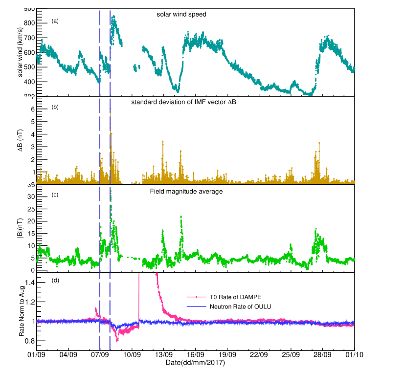
Figure 1: The 5-min averaged time profiles of the solar wind speed (panel (a)), the standard deviation of the IMF vector (panel (b)), the averaged strength of the IMF at 1 AU (panel (c)). Data in panel(a)(b)(c) are all from the OMNI database(https://omniweb.gsfc.nasa.gov/form/omni_min.html). Panel(d) shows the 47-min averaged temporal variation of T0 counting rate of DAMPE for $4.76<L<5.57$ (Rate is normalized to averaged value in August 2017). Also shown in the panel (d) is the OULU NM 10-min averaged relative counting rate with respect to averaged value in August 2017 (data from http://www01.nmdb.eu/nest/). The two vertical red lines indicate the arrival times of the interplanetary shocks.

During the on-orbit operation of DAMPE, the housekeeping system records GCRs trigger counts every 4 seconds (named T0 trigger count) for the purpose of monitoring the health of detectors. T0 is a low threshold hit signal acting as the timing reference to decide to start an event data taking. Based on Geant4 simulation, GCRs with kinematic energy above 100MeV can satisfy the T0 trigger logic. Due to T0 does not record information of particle species, its counting rate only reflects the overall intensity of all kinds of GCRs above 100MeV. On DAMPE’s orbit, the T0 counting rate changes from several hundred Hz near the equator to several thousand Hz at poles. We would like to compare the DAMPE T0 counting rate with the NM data. Since the NMs are fixed on the surface of the Earth, and DAMPE keeps moving along its orbit, we select the T0 counting rate in a narrow region with specific MacIlwain L-parameter values (Walt, 2005) in there geomagnetic cutoff rigidity is assumed to be a constant. For the OULU NM we adopt in the comparison, we find that for $4.76<L<5.57$ the averaged cutoff rigidity is $R_{c}\approx 0.81$ GV which is similar with that of the OULU station. The panel (d) of Figure 1 shows the time evolutions (normalized to the average values in August, 2017) of the DAMPE T0 rate (red) and the OULU NM rate (blue) in September, 2017. A 27 days long-term shallow change of the T0 rate has been subtracted through dividing the rate by a smooth polynomial fitting form to the T0 counts from August 23 to September 24 after abandoning the FD time range. Also shown in Figure 1 are 5-min averaged time profiles of the solar wind speed (panel (a)), the standard deviation of the interplanetary magnetic field (IMF) vector (panel (b)), and the average strength of the IMF (panel (c)). Two vertical lines label the arrival times of two interplanetary shocks, at 23:02 UT, September 6, 2017 and 22:28 UT, September 7, 2018.

From the T0 counting rate, we can clearly identify two solar energetic particle (SEP) events. The first one with smaller amplitude reached the Earth $10-11$ hours before the interplanetary shock wave and lasted for about 20 hours. However, the NM data (from OULU and others) did not show such a rising for this event (see panel (d) of Figure 1). The reason of the difference between NMs and the direct measurements is unclear yet. To a certain extent, DAMPE is not blocked by the atmosphere and is more sensitive to low-energy particles than NM stations. The other possible reason is the anisotropy of SEPs which may lead to missing of the detection by NMs. We also investigate the time profiles of the T0 counts at high latitudes (with $L>4.11$) in both southern and northern hemispheres, and such intensity enhancements are both observed. About 89 hours after the arrival of the second shock (during the recovery phase of the FD), the T0 counting rate further shows a sudden and big jump (increased by 2 orders of magnitude), which indicates the arrival of the second SEP event. At that moment the OULU NM also observed a GLE event with several percents increase of the counting rate. The big difference of the SEP amplitudes between DAMPE and OULU is again a reflection that NMs are only sensitive to high enough energy particles.

During SEPs passbying the Earth (UT 0906-23:02 to 0910-16:03) the fluxes of energetic particles are so high that the detector cannot operate in the normal status any more with significant and random shifts of the pedestals of the electronics. Thus the science data taken in this period has been excluded in the current analysis.

3.2 CRE fluxes

For the purpose of this study, about 60 days of the DAMPE data, in total 300 million events, recorded in August and September 2017 are analyzed. To make sure the detector operates with good condition, the data recorded when DAMPE passes through the South Atlantic Anomaly (SAA) region are excluded.

We apply a series of selection criteria to filter a clean sample of CREs. The purpose is to suppress the background cosmic rays as much as possible while keeping a sufficiently high CRE efficiency. The first step of the pre-selections is to require that the BGO bar with the maximum deposited energy in each layer is not at the edge of the BGO calorimeter, which can make sure that most of the shower energies are recorded by the calorimeter and a good energy resolution is guaranteed. Then a very similar track selection and evaluation strategy as described in Xu et al. (2018) is adopted to identify the tracks of events. Specifically, the STK track should be a long track crossing all layers of STK and matches the BGO track, and the CRE should deposit most energy within a 5mm cylinder around the track. Once the track is determined, the charge of the particle can be obtained via the charge reconstruction algorithm (Dong et al., 2019). Here we require that the charge number measured by PSD should be less than 1.7, which can reject $Z\geq 2$ nuclei up to a level of $99\%$. Finally, to eliminate secondary particles generated in the atmosphere, the minimum energy at each geomagnetic latitude is required to exceed 1.2 times of the vertical rigidity cutoff (VRC; Smart & Shea, 2005).

The pre-selections can already strongly exclude heavy nuclei from the sample. However, there is still heavy contamination from protons and also helium nuclei. Based on the shower development in the calorimeter, a particle identification (PID) variable is constructed.

$${\rm PID}=F(E)[\log({\rm RMS}_{r})\sin\theta+\log({\rm RMS}_{l})\cos\theta]$$

where, $F(E)$ is energy decoupling polynomial, $\theta$ is coordinate rotation angle, ${\rm RMS}_{r}$ and ${\rm RMS}_{l}$ are functions describing radial shower shape and longitudinal shower shape respectively.

The background contamination can then be estimated through a fitting with Monte Carlo (MC) templates in each energy bin, as illustrated in Figure 2. The background contamination is estimated to be $2\%\sim 8\%$ for events with deposited energies between 2 GeV and 20 GeV. Below 2 GeV, the granularity of the calorimeter does not allow us to efficiently identify CREs from nuclei. Since the low energy particles are modulated by solar winds, their fluxes show slight and continuous variations with time. We thus estimate the background in each time bin. It is found that the hadronic background varies by $\sim 6\%$ at 2 GeV and $\sim 1\%$ at 20 GeV. After the pre-selections and the PID procedure, the CRE candidate events are divided into 25 logarithmically even energy bins from 2 GeV to 20 GeV and 240 time bins (6 hours each). The statistical errors in two-dimensional bins are about $2\%$ at 5 GeV and $\sim 8\%$ at 20 GeV.

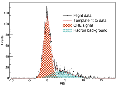
Figure 2: Distributions of the PID variable for deposited energy bin $4.83$ GeV$<E<5.25$ GeV. The best-fit MC templates are also shown for comparison. Setting the PID selection value of $<2$ results in a background contamination of $\sim 8\%$.

Due to the shielding effect of the geomagnetic field, primary GCRs can only be detected when their rigidities are larger than the cutoff rigidity. A threshold of $1.2\times$VRC is adopted to minimize such an effect. Since the VRC varies with locations of the detector, the effective exposure time thus changes with particle rigidity/energy. In each energy bin and time bin, the exposure time is calculated via summarizing the time when the satellite travels in the regions with VRC values smaller than 1/1.2 of the lower edge of the energy bin, with an additional subtraction of the dead time of the DAQ system and the time when DAMPE passes through the SAA region or under the calibration operations. On average the effective exposure time is about $80\%$ of the total time for energies above 15 GeV, which gradually decreases to $\sim 30\%$ at 2 GeV.

The CRE flux in the $i$th energy bin and $j$th time bin can be calculated as

$$\Phi_{i,j}=\frac{N_{i,j}(1-f_{i,j})}{A_{i}\eta_{i,j}\Delta T_{j}\Delta E_{i}},$$ (1)

where $N_{i,j}$, $f_{i,j}$, and $\eta_{i,j}$ represent the number of CRE candidates, the fraction of the background contamination, and the trigger efficiency, $A_{i}$ is the effective acceptance of the detector, $\Delta T_{j}$ is the live time, and $\Delta E_{i}$ is the width of the energy bin. In this analysis we focus on the relative fluxes of CREs in a time scale of two months, and therefore the absolute efficiences are not crucial.

The dominating systematic uncertainty of the relative flux ratio measurements comes from the stability of efficiencies. An extensive study of the efficiency variations have been performed in this analysis. As shown in Ambrosi et al. (2019), the major calibration parameters, including the pedestals, dynode ratios, electronics gains, MIP energies etc., are very stable after the temperature correction (with variations $<1.5$% per year). Therefore the detection efficiency change within one month is expected to be very small ($0.13\%$). On the other hand, due to the radiation damage and electronics aging, the light yields of the BGO crystals and the gains of photomultipliers are found to slightly decrease over time. Their impacts on the trigger threshold of each BGO crystal are carefully calibrated, which show a decrease of $\sim 1.25\%$ per year. We further investigate the impact of the trigger efficiency from the potential bias of the energy scale through applying a series of bias factors from $-5\%$ to $+5\%$ with a step of $1\%$ in the MC simulation, and find that the change of trigger efficiency within 1 month is also small ($0.5\%@2GeV,0.01\%@20GeV$). The other efficiency is the track efficiency of the STK. Since we employ track selection at different moments of 2017, we estimate the corresponding stability of the tracking, using proton flight data samples. Our results confirm the high stability of the tracking efficiency, with the overall variations throughout the data taking period less than $0.2\%$ per year.

In summary, the total systematic uncertainty of the relative detection and selection efficiencies is about $0.53\%$, which is much smaller than the statistical errors ($2\%\sim 8\%$).

4 Time Profiles of CRE fluxes

We calculate the CRE fluxes with a time bin width of 6 hours (about 4 orbits for DAMPE). The flux of each bin is normalized to the average flux of August, 2017. The time profiles of 4 selected energy bins are shown in Figure 3. As we have discussed in Sec. 3.1, the data from 18:00UT of September 9 to 12:00UT of September 11 have been eliminated due to the strong impact from the energetic particles from the SEP. The relative intensities averaged over 10 minutes from the OULU NM are also plotted in Figure 3.

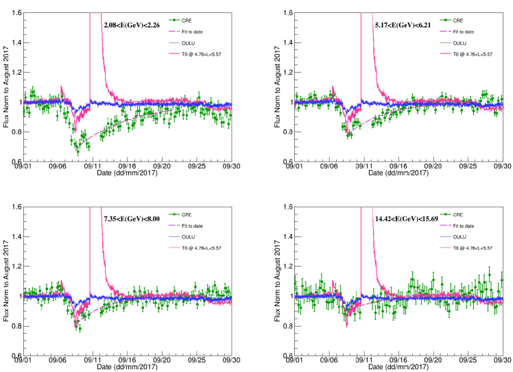
Figure 3: Time profiles of CRE fluxes in four energy bins from 00:00 UT of September 1 to 00:00 UT of October 1, 2017. The error bars are summation of statistical errors and systematic errors. In each plot, the T0 counting rates for $4.76<L<5.57$ are shown in red and the OULU NM intensities are in blue.

Compared with the T0 rates, we do not find significant increase in the CRE fluxes during first SEP event. One possible reason is that the data statistics is limited, and the population of SEP above GeVs is not significant. The NM data do not show the SEP event either. The physical interpretation of such differences may need further studies.

Similar with the PAMELA experiment (Munini et al., 2018) we use the following function

$$\frac{\Phi(t)}{\Phi_{\rm ref}}=1-A_{e}\exp\left(-\frac{t-t_{0}}{\tau}\right),$$ (2)

to describe the amplitude and recovery behavior after the CRE fluxes reach the valley. In the above equation, $\Phi_{\rm ref}$ is the reference flux of August, 2017, $A_{e}$, $\tau$, and $t_{0}$ represent the decrease amplitude, recovery time, and time of the minimum flux (or the start of recovery phase), respectively. For this event, $t_{0}$ is fixed to be 13:30 UT of September 8, 2017. $A_{e}$ and $\tau$ parameters are fitted for each energy bin. The fitting results of the 25 energy bins of $A_{e}$ and $\tau$ are shown in Figure 4. Both $A_{e}$ and $\tau$ clearly show decreases with energy. An exponential decay function, $p_{0}\exp(-E/p_{1})$, is adopted to fit the energy-dependences of $A_{e}$ and $\tau$, resulting in $\chi^{2}/{\rm ndf}=21.45/25$ and $\chi^{2}/{\rm ndf}=34.42/25$, respectively.

The amplitude can be well described by the exponential function. The fact that the FD amplitudes become smaller for higher energies can be easily understood as that high energy particles are less affected by the perturbed interstellar environment by the CME. Consequently, the energy spectra should also vary with time when an FD occurs (Belov et al., 2021), which are expected to be harder during the FD. A single power-law fit to the energy spectrum between 4 and 20 GeV shows that the spectral index is about $2.85$ before the FD, $\sim 2.70$ when the fluxes reach the minimum, and becomes $2.85$ after the FD. The energy-dependence of the recovery time is, however, more complicated than the amplitude. It is interesting to compare the results obtained in this study with that by PAMELA. In Munini et al. (2018), the PAMELA experiment gave the energy-dependences of the recovery time for electrons, protons, and helium nuclei, for rigidities from 0.6 GV to 10 GV. The qualitative behaviors of recovery time for these three types of particles are similar, all show an increase from 0.6 GV to 5 GV, although the specific values for electrons are different from that for nuclei. At higher energies, the recovery time for protons and helium nuclei decreases again. Due to the limited statistics, the decreasing behavior of the electron recovery time has not been observed. The DAMPE result shows clearly the decreasing behavior for the CRE recovery time above 2 GeV, which may indicate that the peaks of the recovery time for all particles are few GeV. We can further see from Figure 4 that at high energies, the recovery time tends to be a constant rather than keeping on decreasing. The recovery time for protons by PAMELA may also show such a flattening at high energies (Munini et al., 2018). But the errors, both for PAMELA protons and DAMPE CREs, are too large to clearly address this phenomenon.

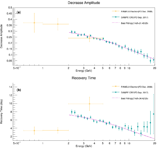
Figure 4: The decease amplitude (panel (a)) and recovery time (panel (a)) versus energy. Red solid lines show the best-fits with an exponential function $p_{0}\exp(-E/p_{1})$.

The ground NMs can also measure the energy-dependences of the FDs, although the energy resolution is relatively poor and the energy threshold is relatively high. As illustrated in Zhao & Zhang (2016), there are two types of energy-dependences of the recovery time, one depends strongly on energies and the other remains almost independent of energies. It has been conjected that the orientations and topologies of the CMEs may result in such differences (Zhao & Zhang, 2016). However, a reliable energy determination of the NMs is difficult. For specific NM station, a typical median energy $E_{M}$ is defined as the value below which cosmic rays contribute to one half of the counting rate. The median energy can be estimated as a function of cutoff rigidity $R_{c}$ as $E_{M}=0.0877R^{2}_{c}+0.154R_{c}+10.12$, where $E_{M}$ and $R_{c}$ are in units of GeV and GV (Jämsén et al., 2007). The median energy is $\sim 10$ GeV at the polar region and $\sim 20$ GeV at the equator. The full behaviors of the recovery time in a wide energy range, especially for lower energies, are thus difficult to be revealed by the NMs. The energy-dependence or independence of the recovery time shown by NMs may be only a part of the full energy-dependence. For the event we discuss here, the CME travels towards the Earth. It should correspond to the Event 2 of Zhao & Zhang (2016), and the recovery time is expected to be a constant. Our results do not support such an expectation in general. However, the constant behavior may just be the reflection of the flattening above $\sim 10$ GeV as shown in Figure 4. A more complete modeling of the recovery time versus energies is necessary.

5 Modeling of the CRE FDs

The Parker’s equation has been widely employed to describe the transport of charged particles in the heliosphere (Parker, 1965). When the heliosphere has been disturbed by CMEs and the associated shocks, FDs of GCR fluxes can occur. This process can be modelled using the diffusion barrier model, which employs a moving diffusion barrier with different diffusion and drift parameters from those in the interplanetary space (Luo et al., 2018). The Parker’s transport equation together with the diffusion barrier can be solved with the stochastic differential equation method (Zhang, 1999; Strauss et al., 2011). We describe the method of the modeling of FDs in detail in the Appendix.

Given proper parameters of the model, the FD behaviors of the DAMPE data can be reproduced, as shown in Figure 5 for selected energy bands. We further derive the recovery time at different energies using Eq.(2), and give the results in Figure 6. We can see that the model prediction is in good agreement with the data in the energy range of $2-20$ GeV. However, this model may not explain precisely the detailed behaviors of the data at higher or lower energies. The possible flattening at high energies, although higher precision of the measurements is required to reach a conclusion, is not obvious in the modeling. Also the model predicts longer recovery time at lower energies, which may not explain the turnover at few GeV as indicated by the PAMELA and DAMPE data. Further refinement or modification of the FD modeling is thus necessary to fully account for the data.

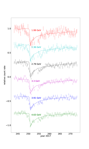
Figure 5: Variations of the relative CRE fluxes from the DAMPE observations (bars) and the FD model (lines). For visualization the results for different energies are shifted downwards gradually with respect to the top one in each panel.

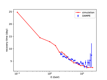
Figure 6: The recovery time of the model prediction compared with the DAMPE data.

6 Conclusion

In this work we give a detailed study of the FDs of CREs associated with the CME occurred in September, 2017 by the DAMPE detector. A weak SEP event has been revealed through the T0 counting rate, while no unambiguous signal is shown by on-ground NMs. Meanwhile the high-precision time evolutions of CRE fluxes with a 6-hour time resolution have been obtained simultaneously. We study the energy-dependences of the FD amplitudes and the recovery time, and find that both decrease with energies. Together with the results of different particle species measured by PAMELA, it may show that the recovery time of all species of particles show an increase below a few GeV and a decrease at higher energies. For energies above $\sim 10$ GeV, the recovery time may become constant, which nevertheless requires more statistics to draw a firm conclusion. These results would give very important implications in modeling the propagation of GCRs in the heliosphere when there are disturbances from CMEs.

This study also illustrates the importance of direct measurements of FDs of various GCR species. Compared with the usually employed NM data, the direct measurements have the advantages of excellent particle identification, very good energy resolution, and much wider energy range coverage. More comparative studies of various FD events for different particle species by DAMPE in future are expected to further shed light on the understanding of the physics of particle transportation in the interplanetary environment.

Appendix A The Parker’s transport equation

The Parker’s transport equation is written as (Parker, 1965)

$$\frac{\partial f}{\partial t} = -~{}\left(\vec{V}_{\rm sw}+\left\langle\vec{v}_{d}\right\rangle\right)\cdot\nabla f$$

$$+ \nabla\cdot\left(K^{(s)}\cdot\nabla f\right)$$

$$+ ~{}\frac{1}{3}\left(\nabla\cdot\vec{V}_{\rm sw}\right)\frac{\partial f}{\partial\ln p},$$ (A2)

where $f(\vec{r},p,t)$ is the particle distribution function, $p$ is the momentum, $\vec{V}_{\rm sw}$ is the latitude-dependent solar wind speed (Potgieter et al., 2015; Luo et al., 2019), $\left\langle\vec{v}_{d}\right\rangle$ is the pitch-angle averaged drift velocity (Jokipii et al., 1977; Burger & Potgieter, 1989; Forman et al., 1974; Engelbrecht & Burger, 2015) with the following form:

$$\left\langle\vec{v}_{d}\right\rangle=\frac{pv}{3q}\nabla\times\frac{\vec{B}}{B^{2}},$$ (A3)

where $q$ and $v$ are the charge and velocity of the GCR particle, and $\vec{B}$ is the magnetic field inside the heliosphere. The last term of Eq.(A) is the adiabatic energy loss. $K^{(s)}$ is the symmetric diffusion tensor, given in the IMF aligned coordinates by

$$K^{(s)}=\left(\begin{array}[]{ccc}\kappa_{\parallel}&0&0\\ 0&\kappa_{\perp\theta}&0\\ 0&0&\kappa_{\perp r}\\ \end{array}\right),$$ (A4)

where $\kappa_{\parallel}$ is the parallel diffusion coefficient, and $\kappa_{\perp r}$, $\kappa_{\perp\theta}$ are two perpendicular diffusion coefficients in the radial and latitudinal directions. In our simulation, the diffusion coefficients are expressed as (Luo et al., 2019)

$$\kappa_{\parallel}=\kappa_{\parallel 0}\beta\frac{B_{0}}{B}\left(\frac{P}{P_{k}}\right)^{a}\left[1+\left(\frac{P}{P_{k}}\right)^{\frac{b-a}{c}}\right]^{c},$$ (A5)

$$\kappa_{\perp r,\perp\theta}=(\kappa_{\perp r0,\perp\theta 0})\beta\frac{B_{0}}{B}\left(\frac{P}{P_{k}}\right)^{a}\left[1+\left(\frac{P}{P_{k}}\right)^{\frac{b-a}{c}}\right]^{c}.$$ (A6)

Here, $\beta$ is the particle velocity in unit of the light speed, $B$ is the magnitude of the local IMF with $B_{0}=1$ nT, $P$ is the rigidity, $\kappa_{\parallel 0}$, $\kappa_{\perp r0}$, and $\kappa_{\perp\theta 0}$ are constants, $P_{k}$, $a$, $b$, $c$ are free parameters which define the rigidity dependence of these diffusion coefficients.

We use the standard Parker field to describe the IMF (Parker, 1958):

$$\vec{B}(r,\theta)=\frac{AB_{\oplus}}{r^{2}}\left(\boldsymbol{e_{r}}-\frac{r\Omega\sin\theta}{V_{\rm sm}}\boldsymbol{e_{\theta}}\right)\left[1-2H(\theta-\theta_{\rm cs})\right],$$ (A7)

where $B_{\oplus}$ is the reference value at the earth position which we take as the mean value of the last 13 months before the solar flare event, $A=\pm 1/{\sqrt{\left(1+\frac{\Omega^{2}}{\vec{V}_{\rm sw}^{2}}\right)}}$ with the sign determining the polarity of the IMF, $\Omega$ is the angular velocity of the Sun, $H(\theta-\theta_{\rm cs})$ is the Heaviside function and $\theta_{\rm cs}$ determines the polar extent of the Heliospheric Current Sheet (HCS). We model the HCS by the following analytical expression (Kota J, Jokipii JR, 1983),

$$\cot\theta_{\rm cs}=-\tan\alpha~{}\sin\phi^{*}.$$ (A8)

Here, $\alpha$ is the HCS tilt angle which we also adopt as the mean value of the last 13 months, $\phi^{*}=\phi+\frac{r\Omega}{V_{\rm sw}}$ with $\phi$ being the longitude angle of the current sheet surface. We do not consider the phase of the co-rotating HCS.

The the magnitude of drift in the HCS can be specified as (Burger & Potgieter, 1989)

$$v_{\rm HCS}=\frac{v}{6}\times\frac{4R_{g}}{r}\delta(\theta-\theta_{\rm cs}),$$ (A9)

where $R_{g}$ is the gyroradius of the GCR particle and $v$ is the particle’s speed. Following Luo et al. (2013) and Luo et al. (2017), we replace $\delta(\theta-\theta_{\rm cs})$ with $r/(4R_{g})$ within the distance of $(-2R_{g},2R_{g})$ to the HCS. By defining $\psi$ as the angle between the local current sheet normal direction $\boldsymbol{n}$ and the $-\boldsymbol{e_{\theta}}$ direction, the drift vector of the current sheet can be written as

$$\vec{V}_{\rm cs}=\frac{v}{6}\left(\boldsymbol{e_{r}}\sin{\Phi}\cos\psi+\boldsymbol{e_{\theta}}\sin\psi+\boldsymbol{e_{\phi}}\cos\Phi\cos\psi\right),$$ (A10)

with $\Phi$ being the IMF winding (spiral) angle.

Appendix B The diffusion barrier model

In our model, we use a 3D geometry profile to describe the propagating diffusion barrier. The diffusion and drift coefficients inside the barrier are expressed as

$$\kappa^{\prime}_{\parallel,\perp,T}=\frac{\kappa_{\parallel,\perp,T}}{1+\rho h(\theta)f(r)g(\phi)}.$$ (B1)

In the above equation, $\kappa^{\prime}_{\parallel,\perp}$ ($\kappa^{\prime}_{T}$) are the diffusion (drift) coefficients inside the barrier, $\rho$ is a constant determining the reduction level of the diffusion and drift coefficients, $h(\theta)$, $g(\phi)$, and $f(r)$ describe the geometry of the diffusion barrier

$$h(\theta) = e^{-\left(\frac{\theta-\theta_{0}}{\theta_{\rm br}}\right)^{10}},$$ (B2)

$$g(\phi) = e^{-\left(\frac{\phi}{\phi_{\rm br}}\right)^{10}},$$ (B3)

$$f(r) = \left\{\begin{array}[]{lc}1-\frac{r-r_{\rm cen}}{r_{\rm a}},&r_{\rm cen}<r<r_{\rm sh}\\ \frac{r-r_{\rm end}}{r_{\rm b}},&r_{\rm end}<r\leq r_{\rm cen}\\ 0,&{\rm otherwise}\end{array}\right..$$ (B7)

Here, $\theta_{0}=\pi/2$ means that diffusion barrier hits the earth head on, the parameters $\theta_{\rm br}$ and $\phi_{\rm br}$ denote the extensions of the diffusion barrier along the $\boldsymbol{e_{\theta}}$ and $\boldsymbol{e_{\phi}}$ directions, $r_{\rm sh}$, $r_{\rm cen}$, and $r_{\rm end}$ are the radial distances of the front, center, and end locations of the barrier, $r_{\rm a}=r_{\rm sh}-r_{\rm cen}$, $r_{\rm b}=r_{\rm cen}-r_{\rm end}$ are widths of the leading and trailing paths of the barrier. In our model, we assume $r_{\rm a}=0.5$ AU, $r_{\rm b}=0.3$ AU, $\theta_{\rm br}=60^{\circ}$, $\phi_{\rm br}=180^{\circ}$. The velocity of the diffusion barrier is adopted to be 1500 km/s, as given in the CME list.

Appendix C The stochastic differential equation method

Based on the Ito’s formula, the Parker’s equation can be solved numerically with the stochastic differential equation (SDE) technique (Zhang, 1999; Strauss et al., 2011), with

$$d\vec{X}=\left(\nabla\cdot K^{(s)}-\vec{V_{\rm sw}}-\left\langle\vec{v}_{d}\right\rangle\right)ds+\sum^{3}_{\sigma=1}\vec{\alpha}_{\sigma}dW_{\sigma}(s),$$ (C1)

$$dp=\frac{p}{3}(\nabla\cdot\vec{V}_{\rm sw}\,ds),$$ (C2)

where $dW_{\sigma}(s)$ is the Wiener process, which can be numerically generated by the Gaussian random number, and $\sum_{\sigma}{\alpha}_{\sigma}^{\mu}\alpha_{\sigma}^{\nu}=2\kappa^{\mu\nu}$. The SDE method gives the time-dependent solution of Eq. (A) as (Zhang, 1999; Luo et al., 2019)

$$f(t,\vec{X},p)=\left\langle f_{b}^{i}(t-\chi_{i},\vec{X}_{i},p_{i})\right\rangle.$$ (C3)

$\left\langle f_{b}^{i}(t-\chi_{i},\vec{X}_{i},p_{i})\right\rangle$ is the mean value for the pseudo-particles reaching the boundary $(\vec{X}_{i},p_{i})$ at the first exit time $\chi_{i}$. In our calculation, the local interstellar spectrum of electrons are adopted from Zhu et al. (2021). The small fraction of positrons has been neglected.

References

- Ambrosi et al. (2019) Ambrosi, G., An, Q., Asfandiyarov, R., et al. 2019, Astroparticle Physics, 106, 18
- An et al. (2019) An, Q., Asfandiyarov, R., Azzarello, P., et al. 2019, Science Advances, 5, eaax3793. https://arxiv.org/abs/1909.12860
- Azzarello et al. (2016) Azzarello, P., Ambrosi, G., Asfandiyarov, R., et al. 2016, Nuclear Instruments and Methods in Physics Research Section A, 831, 378
- Badruddin et al. (2019) Badruddin, B., Aslam, O. P. M., Derouich, M., Asiri, H., & Kudela, K. 2019, Space Weather, 17, 487
- Belov et al. (2021) Belov, A., Papaioannou, A., Abunina, M., et al. 2021, The Astrophysical Journal, 908, 5, doi: 10.3847/1538-4357/abd724
- Burger & Potgieter (1989) Burger, R. A., & Potgieter, M. S. 1989, The Astrophysical Journal, 339, 501
- Burlaga (2015) Burlaga, L. 2015, Journal of Physics: Conference Series, 642, 012003
- Chang et al. (2017) Chang, J., Ambrosi, G., An, Q., et al. 2017, Astroparticle Physics, 95, 6, doi: 10.1016/j.astropartphys.2017.08.005
- Chertok et al. (2018) Chertok, I. M., Belov, A. V., & Abunin, A. A. 2018, Space Weather, 16, 1549
- DAMPE Collaboration et al. (2017) DAMPE Collaboration, Ambrosi, G., An, Q., et al. 2017, Nature, 552, 63, doi: 10.1038/nature24475
- Dong et al. (2019) Dong, T., Zhang, Y., Ma, P., et al. 2019, Astroparticle Physics, 105, 31. https://arxiv.org/abs/1810.10784
- Engelbrecht & Burger (2015) Engelbrecht, N. E., & Burger, R. A. 2015, Advances in Space Research, 55, 390
- Forbush (1937) Forbush, S. E. 1937, Phys. Rev., 51, 1108
- Forman et al. (1974) Forman, M. A., Jokipii, J. R., & Owens, A. J. 1974, The Astrophysical Journal, 192, 535
- Guo et al. (2018) Guo, J., Lillis, R., Wimmer-Schweingruber, R. F., et al. 2018, Astronomy & Astrophysics, 611, A79
- Hess & Demmelmair (1937) Hess, V. F., & Demmelmair, A. 1937, Nature, 140, 316
- Huang et al. (2020) Huang, Y.-Y., Ma, T., Yue, C., et al. 2020, Research in Astronomy and Astrophysics, 20
- Hubert et al. (2019) Hubert, G., Pazianotto, M. T., Federico, C. A., & Ricaud, P. 2019, Journal of Geophysical Research: Space Physics, 124, 661
- Jämsén et al. (2007) Jämsén, T., Usoskin, I. G., Räihä, T., Sarkamo, J., & Kovaltsov, G. A. 2007, Advances in Space Research, 40, 342, doi: 10.1016/j.asr.2007.02.025
- Jokipii et al. (1977) Jokipii, J. R., Levy, E. H., & Hubbard, W. B. 1977, The Astrophysical Journal, 213, 861
- Kota J, Jokipii JR (1983) Kota J, Jokipii JR. 1983, The Astrophysical Journal, 265, 573
- Livada & Mavromichalaki (2020) Livada, M., & Mavromichalaki, H. 2020, Solar Physics, 295
- Luo et al. (2019) Luo, X., Potgieter, M. S., Bindi, V., Zhang, M., & Feng, X. 2019, The Astrophysical Journal, 878, 6. https://arxiv.org/abs/1909.03050
- Luo et al. (2017) Luo, X., Potgieter, M. S., Zhang, M., & Feng, X. 2017, The Astrophysical Journal, 839, 53
- Luo et al. (2018) Luo, X., Potgieter, M. S., Zhang, M., & Feng, X. 2018, The Astrophysical Journal, 860, 160
- Luo et al. (2013) Luo, X., Zhang, M., Feng, X., & Mendoza-Torres, J. E. 2013, Journal of Geophysical Research (Space Physics), 118, 7517
- Ma et al. (2019) Ma, P.-X., Zhang, Y.-J., Zhang, Y.-P., et al. 2019, Research in Astronomy and Astrophysics, 19, 082. https://arxiv.org/abs/1808.05720
- Munini et al. (2018) Munini, R., Boezio, M., Bruno, A., et al. 2018, The Astrophysical Journal, 853, 76
- Parker (1965) Parker, E. 1965, Planet. Space Sci., 13, 9
- Parker (1958) Parker, E. N. 1958, The Astrophysical Journal, 128, 664
- Peter Meyer, Rochus Vogt (1961) Peter Meyer, Rochus Vogt. 1961, Journal of Geophysical Research, 66, 3950, doi: 10.1029/JZ066i011p03950
- Potgieter et al. (2015) Potgieter, M. S., Vos, E. E., Munini, R., Boezio, M., & Di Felice, V. 2015, The Astrophysical Journal, 810, 141
- Smart & Shea (2005) Smart, D. F., & Shea, M. A. 2005, Advances in Space Research, 36, 2012
- Strauss et al. (2011) Strauss, R. D., Potgieter, M. S., Büsching, I., & Kopp, A. 2011, The Astrophysical Journal, 735, 83
- Tykhonov et al. (2018) Tykhonov, A., Ambrosi, G., Asfandiyarov, R., et al. 2018, Nuclear Instruments and Methods in Physics Research A, 893, 43. https://arxiv.org/abs/1712.02739
- Tykhonov et al. (2019) —. 2019, Nuclear Instruments and Methods in Physics Research A, 924, 309
- Walt (2005) Walt, M. 2005, Introduction to Geomagnetically Trapped Radiation, by Martin Walt, pp. . ISBN 0521616115. Cambridge, UK: Cambridge University Press, 2005., -1
- Xu et al. (2018) Xu, Z.-L., Kaikai, D., Shen, Z.-Q., et al. 2018, Research in Astronomy and Astrophysics, 18, 027
- Yu et al. (2017) Yu, Y., Sun, Z., Su, H., et al. 2017, Astroparticle Physics, 94, 1. https://arxiv.org/abs/1703.00098
- Zhang (1999) Zhang, M. 1999, The Astrophysical Journal, 513, 409
- Zhang et al. (2015) Zhang, Z., Zhang, Y., Dong, J., et al. 2015, Nuclear Instruments and Methods in Physics Research A, 780, 21
- Zhang et al. (2016) Zhang, Z., Wang, C., Dong, J., et al. 2016, Nuclear Instruments and Methods in Physics Research A, 836, 98. https://arxiv.org/abs/1602.07015
- Zhao & Zhang (2016) Zhao, L. L., & Zhang, H. 2016, The Astrophysical Journal, 827, 13
- Zhu et al. (2021) Zhu, C. R., Yuan, Q., & Wei, D. M. 2021, Astroparticle Physics, 124, 102495