Real-Time Evolution in the Hubbard Model with Infinite Repulsion

Abstract

We consider the real-time evolution of the Hubbard model in the limit of infinite coupling. In this limit the Hamiltonian of the system is mapped into a number-conserving quadratic form of spinless fermions, i.e. the tight binding model. The relevant local observables, however, do not transform well under this mapping and take very complicated expressions in terms of the spinless fermions. Here we show that for two classes of interesting observables the quench dynamics from product states in the occupation basis can be determined exactly in terms of correlations in the tight-binding model. In particular, we show that the time evolution of any function of the total density of particles is mapped directly into that of the same function of the density of spinless fermions in the tight-binding model. Moreover, we express the two-point functions of the spin-full fermions at any time after the quench in terms of correlations of the tight binding model. This sum is generically very complicated but we show that it leads to simple explicit expressions for the time evolution of the densities of the two separate species and the correlations between a point at the boundary and one in the bulk when evolving from the so called generalised nested Néel states.

I Introduction

The Hubbard model is the fundamental paradigm of strongly correlated electrons and, as such, is attracting the attention of theoreticians from many different corners of condensed matter. In particular, the 1D version of the Hubbard model is at the focus of the theoretical activity ever since Lieb and Wu discovered its Bethe Ansatz integrability lieb1968absence . In the context of many-body systems, however, integrability does not mean simplicity: the models solved by Bethe-Ansatz generically retain non-trivial interactions and many interesting quantities — most importantly correlations functions — remain inaccessible in most cases. Moreover, the Bethe Ansatz solution of the 1D Hubbard model is particularly complicated from the technical point of view: it involves two intertwined sets of Bethe equations, i.e. it is nested in the technical parlour, and its R-matrix is not in difference form essler2005one . In spite of this mathematical complexity, however, a remarkable collective effort led to a comprehensive description of its equilibrium thermodynamics culminating in a complete account of its rich phase diagram essler2005one .

A natural next step is then to understand the 1D Hubbard model out of equilibrium. Indeed, a substantial body of work distributed over the last 15 years (see, e.g., the reviews in the volumes cem-16 ; bastianello2021special ) has revealed that, when driven out of equilibrium, integrable models display rich and interesting physics. For instance, in homogeneous settings, local observables in out-of-equilibrium integrable models relax to values described by the generalised Gibbs Ensemble (GGE) RigolPRL07 ; vidmar2016generalised rather than the standard thermal ensemble expected for non-integrable systems D91 ; S94 . The GGE is a statistical ensemble built with of all the local and quasi-local conserved charges of the Hamiltonian cef-ii ; IDWC15 , which are extensively many in integrable models. Therefore, the GGE retains extensive memory about the initial configuration. The exact knowledge of the stationary state allows one to compute stationary values of observables without solving the overwhelmingly complicated many-body dynamics and, moreover, it also gives access the asymptotic dynamics of correlations bonnes-2014 and entanglement ac-16 ; ac-17 ; c-20 . Importantly, the occurrence of GGEs has also been observed experimentally langen-2015 .

Another remarkable breakthrough has been the discovery that the late time behaviour of integrable systems in inhomogeneous settings is described by a set of hydrodynamic equations involving all the quasi-local charges: such an unconventional hydrodynamic theory has been termed generalised hydrodynamics (GHD) BCDF:transport ; CADY:hydro ; d-ls ; Bertini2021 ; Alba2021 . Despite being macroscopically many, the GHD equations can be treated analytically, allowing for an unprecedented quantitative comparison between theory and experiments Schemmer2019 ; Malvania2020 ; Bouchoule2021 .

Very few of the aforementioned results, however, have so far been explicitly tested in the case of the Hubbard model. This is mainly because none of the analytical approaches developed to determine the stationary state of out-of-equilibrium integrable systems caux_time_2013 ; caux_qareview ; iqdb-16 ; piroli2017what can be applied to the Hubbard model with finite interaction strength due to its technical complexity. In essence, the evolution of the Hubbard model has been accessed only in the quasi-stationary regime using GHD equations ilievski2017ballistic ; fava2020spin , whose solution has been explicitly worked out also for models with a nested Bethe ansatz mbpc-18 ; bpk-19 ; scl-21 ; wyc-20 ; nt-20 ; nt-21 . A promising direction to compute stationary values in the Hubbard model is the so called quench action method caux_time_2013 ; caux_qareview . Indeed, this approach does not require the explicit form of the set of conserved charges and, for this reason, it has been used to obtain exact results even when, like in the Hubbard model, the full charge spectrum was unknown dwbc-14 ; BePC16 ; BeSE14 ; wdbf-14 ; QA:XXZ ; PMWK14 ; mestyan_quenching_2015 ; ac-16qa ; pce-16 ; NaPC15 ; Bucc16 ; npg-17 . A limitation, however, is that this method requires the exact overlaps between the initial state and all the eigenstates of the time-evolving Hamiltonian. These quantities have been accessed only in a few special cases Pozs18 ; HoST16 ; fz-16 ; Broc14 ; PiCa14 ; Pozs14 , including models with nested Bethe ansatz pvcp-18 ; pvcp-18-II , but not (yet) for the Hubbard model with finite interaction strength.

A more general open question concerns the finite-time dynamics of the Hubbard model. Namely the time evolution of the system away from the asymptotic regime. This regime is clearly very interesting — for instance accessing it could reveal the quantitative mechanisms allowing quantum many-body systems to attain local equilibrium — but is largely uncharted in integrable models due to the lack of methods to access it. For instance, although in principle the quench action can provide the full post-quench dynamics caux_time_2013 , this task has to be performed numerically rkc-21 ; dpc-15 , with only few special cases (usually mappable to free systems) where some analytic solutions can be found in full glory caux_time_2013 ; dc-14 ; pc-17 . Interestingly, however, in recent years a number of exact results concerning the finite time dynamics have been found in a special class of integrable systems, which can be thought of as strong coupling limits pozsgay2014quantum ; pozsgay2016real ; klobas2021exact ; zadnik2021the ; zadnik2021the2 ; klobas2021exact2 ; klobas2021entanglement .

In summary, because of its intrinsic difficulty, the non-equilibrium dynamics of the one-dimensional Hubbard model have so far been investigated mainly by numerical or approximate means, see e.g. Refs. mk-08 ; ekw-09 ; sf-10 ; qkns-14 ; ymwr-14 ; roh-15 ; yr-17 ; sjhb-17 ; rcfg-21 . To overcome these difficulties, in Ref. bertini2017quantum we considered the limit of infinite repulsion, when the thermodynamics becomes essentially that of a free model. In this limit, we exploited the quench action approach to build the stationary state for many relatively simple low entangled initial states. The infinite repulsion limit of the Hubbard model has later been considered in Ref. zhang2019quantum , which presented a method able to reconstruct the full time evolution of two-point correlations from a special class of product initial states where the spin has to flip from one particle to the next. The approach of Ref. zhang2019quantum is based on a mapping to non-interacting spinless fermions, developed in Ref. zhang2018impenetrable , that works at the level of the correlations and accounts for their evolution numerically with polynomial complexity in time. In this paper we focus again on the time-evolution of the Hubbard model in the limit of infinite repulsion but reconstruct the dynamics of relevant observables using a different mapping to free fermions. In particular we consider the operatorial mapping introduced by Kumar in Ref. kumar2008canonical ; kumar2008exact . Applying Kumar’s mapping we find explicit analytical expressions for certain relevant correlations. Differently from the results of Ref. zhang2019quantum , our findings can be applied for initial states with generic spin configurations and the explicit expressions that we provide can be evaluated in the thermodynamic limit. On the other hand, being valid for more general initial states, our expressions for generic two-point correlations are more complicated than those found in Ref. zhang2019quantum .

The rest of this manuscript is laid out as follows. In Sec. II we introduce the model and discuss the infinite interaction limit. In Sec. III we provide a detailed review of Kumar’s mapping for the local observables in the infinite repulsion limit. Sec. IV is the core of this manuscript where we use this mapping to obtain the time evolution of several local observables. In Sec. V we summarise our results and discuss some further developments. Two appendices contain some technical details of our calculations.

II Hubbard Model with Infinite Repulsion

We consider a system of interacting spin-full fermions on a one-dimensional lattice whose dynamics are described by the Hubbard Hamiltonian essler2005one , i.e.

$${H}=-J\sum_{x=1}^{L-1}\sum_{\alpha=\uparrow,\downarrow}\left(c_{x,\alpha}^{\dagger}c^{\phantom{\dagger}}_{x+1,\alpha}+c_{x+1,\alpha}^{\dagger}c^{\phantom{\dagger}}_{x,\alpha}\right)+U\sum_{x=1}^{L}\left(n_{x,\uparrow}-\frac{1}{2}\right)\left(n_{x,\downarrow}-\frac{1}{2}\right).$$ (1)

Here we denoted by $\{c_{x,\alpha}\}$ a set of spin-$1/2$ fermionic operators fulfilling the canonical anti-commutation relations

$$\{c_{x,\alpha},c_{y,\beta}\}=\{c_{x,\alpha}^{\dagger},c_{y,\beta}^{\dagger}\}=0,\qquad\{c_{x,\alpha},c_{y,\beta}^{\dagger}\}=\delta_{x,y}\delta_{\alpha,\beta}\,,\qquad\alpha,\beta=\uparrow,\downarrow,$$ (2)

and by $n_{x,\uparrow/\downarrow}$ the local number operators

$$n_{x,\alpha}=c_{x,\alpha}^{\dagger}c_{x,\alpha}.$$ (3)

Moreover we indicated by $L$ is the number of sites of the chain and we adopted open boundary conditions.

The vacuum state is defined in the usual fashion as the state annihilated by the operators $c_{x,\alpha}$

$$c_{x,\alpha}\ket{0}=0,\qquad x=1,2,\ldots,L,\qquad\alpha=\uparrow,\downarrow.$$ (4)

Any site on the lattice can have no particles, a fermion with spin up, a fermion with spin down or two fermions with different spin. These states at site $x$ are constructed by acting with the fermionic creation operators on the vacuum as follows

$$\ket{0},\qquad c_{x,\uparrow}^{\dagger}\ket{0},\qquad c_{x,\downarrow}^{\dagger}\ket{0},\qquad c_{x,\uparrow}^{\dagger}c_{x,\downarrow}^{\dagger}\ket{0}\,.$$ (5)

Since at every site there are $4$ possible states, the total Hilbert space has $4^{L}$ states. We refer to the states with at least one site with two particles as double occupancy states; note that these states are the only ones affected by the interaction term.

In this paper we are interested in the limit of infinite interaction $U\rightarrow\infty$. In this limit, the double occupancy states have infinite energy and, therefore, become unphysical. This limit can be thought of as a limit of infinite repulsion among the fermions as no two particles can sit on the same site. The physical Hilbert space is then the $3^{L}$-dimensional subspace with no double occupancy states. The effective Hamiltonian describing the dynamics in this limit is written as

$$H_{\infty}=-J\,\mathcal{P}\!\left[\sum_{x=1}^{L-1}\sum_{\alpha=\uparrow,\downarrow}\left(c_{x,\alpha}^{\dagger}c^{\phantom{{\dagger}}}_{x+1,\alpha}+c_{x+1,\alpha}^{\dagger}c^{\phantom{{\dagger}}}_{x,\alpha}\right)\right]\!\!\mathcal{P},\qquad\mathcal{P}=\prod_{x=1}^{L}(1-n_{x,\uparrow}n_{x,\downarrow}).$$ (6)

This Hamiltonian is known as the $t$ - 0 model essler2005one and is non-trivial only when the number of particles is less than $L$.

III Kumar mapping to free fermions

Interestingly, as shown by Kumar in Ref. kumar2008exact (see also Refs. kumar2008canonical ; nocera2018finite ), the Hamiltonian (6) is exactly mapped into the tight-binding model by a unitary transformation, i.e.

$$\mathcal{U}^{\dagger}H_{\infty}\mathcal{U}=H_{\rm tb}\equiv-J\sum_{x=1}^{L+1}(f^{\dagger}_{x+1}f^{\phantom{{\dagger}}}_{x}+f^{\dagger}_{x}f^{\phantom{{\dagger}}}_{x+1}),\qquad\qquad\mathcal{U}^{\dagger}\mathcal{U}=\mathcal{U}^{\dagger}\mathcal{U}=I,$$ (7)

where $\{f_{x}\}$ are canonical spinless fermions fulfilling

$$\{f^{\phantom{{\dagger}}}_{x},f^{\phantom{{\dagger}}}_{y}\}=\{f^{\dagger}_{x},f^{\dagger}_{y}\}=0,\qquad\{f^{\dagger}_{x},f^{\phantom{{\dagger}}}_{y}\}=\delta_{x,y}.$$ (8)

This mapping represents the main technical tool of our analysis: In this section we will pedagogically review the three main steps of the mapping, while in Sec. IV we will use it to determine the real-time evolution of interesting observables. Note that Kumar’s mapping has originally been developed in the case of open boundary conditions but, by addressing some additional complications, it has later been extended to the periodic case brzezicki2014topological . Here, however, we stick to the open-chain case for the sake of simplicity.

III.1 Operatorial Mapping

The first step is to define a formal operatorial mapping between the set of spinful fermions $\{c^{\dagger}_{x,\alpha}\}_{\alpha=\uparrow,\downarrow}$ and a set $\{f_{x},\sigma_{a,x}\}_{a=1,2,3}$ composed by canonical spinless fermions $f^{\dagger}_{x}$ fulfilling (8) and Pauli matrices $\{\sigma_{a,x}\}_{a=1,2,3}$. In particular, considering a chain with an even number of sites $L$ we define

$$c^{\dagger}_{x,\uparrow} =a^{x}_{x}\sigma^{\phantom{{\dagger}}}_{+,x}, c^{\dagger}_{x,\downarrow} =\tfrac{1}{2}(\mathrm{i}a^{y}_{x}-a^{x}_{x}\sigma^{\phantom{{\dagger}}}_{3,x}), x\text{ odd}$$ (9a)

$$c^{\dagger}_{x,\uparrow} =\mathrm{i}a^{y}_{x}\sigma^{\phantom{{\dagger}}}_{+,x}, c^{\dagger}_{x,\downarrow} =\tfrac{1}{2}(a^{x}_{x}-\mathrm{i}a^{y}_{x}\sigma^{\phantom{{\dagger}}}_{3,x}), x\text{ even}$$ (9b)

where we introduced the Majorana fermions

$$a^{x}_{x}=f^{\dagger}_{x}+f_{x},\qquad\qquad\mathrm{i}a^{y}_{x}=f^{\dagger}_{x}-f_{x}\,,$$ (10)

and the spin-ladder operators

$$\sigma_{\pm,x}=\frac{\sigma_{1,x}\pm i\sigma_{2,x}}{2}\,.$$ (11)

Under the mapping (9) the states (5) transform as follows

$$\ket{0} \mapsto\ket{\fullmoon}\ket{-}, c_{x,\uparrow}^{\dagger}\ket{0} \mapsto f^{\dagger}_{x}\sigma^{\phantom{{\dagger}}}_{+,x}\ket{\fullmoon}\ket{-},$$ (12)

$$c_{x,\downarrow}^{\dagger}\ket{0} \mapsto f^{\dagger}_{x}\ket{\fullmoon}\ket{-}, c_{x,\uparrow}^{\dagger}c_{x,\downarrow}^{\dagger}\ket{0} \mapsto(-1)^{x+1}\sigma_{+,x}\ket{\fullmoon}\ket{-},$$ (13)

where we respectively denoted by $\ket{\fullmoon}$ and $\ket{-}$ the spinless-fermion vacuum and the spin-down state. These states are defined by

$$f_{x}\ket{\fullmoon}=0,\qquad\qquad\sigma_{-,x}\ket{-}=0,\qquad\qquad\forall x\,.$$ (14)

The explicit form of the inverse of (9) depends on the parity of $x$. In particular, for odd $x$ we have

$$f_{x}^{\dagger} =(1-n_{x,\uparrow})c^{\dagger}_{x,\downarrow}-n_{x,\uparrow}c_{x,\downarrow}\,, \sigma_{3,x} =2n_{x,\uparrow}-1\,, \sigma_{+,x} =c^{\dagger}_{x,\uparrow}(c^{\dagger}_{x,\downarrow}+c^{\phantom{{\dagger}}}_{x,\downarrow})\,,$$ (15a)

$$a^{x}_{x} =(1-2n_{x,\uparrow})(c^{\dagger}_{x,\downarrow}+c^{\phantom{{\dagger}}}_{x,\downarrow})\,, \mathrm{i}a^{y}_{x} =c^{\dagger}_{x,\downarrow}-c^{\phantom{{\dagger}}}_{x,\downarrow}\,,$$ (15b)

while for even $$x$$ we find

$$f_{x}^{\dagger} =n_{x,\uparrow}c^{\dagger}_{x,\downarrow}+(1-n_{x,\uparrow})c^{\phantom{{\dagger}}}_{x,\downarrow}\,, \sigma_{3,x} =2n_{x,\uparrow}-1\,, \sigma_{+,x} =c^{\dagger}_{x,\uparrow}(c^{\dagger}_{x,\downarrow}-c^{\phantom{{\dagger}}}_{x,\downarrow}),$$ (15c)

$$a^{x}_{x} =c^{\dagger}_{x,\downarrow}+c^{\phantom{{\dagger}}}_{x,\downarrow}\,, \mathrm{i}a^{y}_{x} =(1-2n_{x,\uparrow})(c^{\dagger}_{x,\downarrow}-c^{\phantom{{\dagger}}}_{x,\downarrow})\,.$$ (15d)

For future reference we also note the following simple relationship between the local number operators in the spinful and spinless fermions

$$\left(n_{x,\uparrow}-\frac{1}{2}\right)\left(n_{x,\downarrow}-\frac{1}{2}\right)=\frac{1}{2}\left(\frac{1}{2}-d_{x}\right),$$ (16)

where we introduced the local number operator for spinless fermions

$$d_{x}\equiv f^{\dagger}_{x}f^{\phantom{{\dagger}}}_{x}\,.$$ (17)

Finally, applying the mapping (9) to the Hamiltonian (1) one finds

$${H}= -{J}\sum_{x=1}^{L-1}\left[(f^{\dagger}_{x+1}f_{x}+f^{\dagger}_{x}f_{x+1})X_{x,x+1}+(-1)^{x}(f^{\dagger}_{x+1}f^{\dagger}_{x}+f_{x}f_{x+1})(X_{x,x+1}-1)\right]\!-\frac{U}{2}\sum_{x=1}^{L}\left(f^{\dagger}_{x}f_{x}-\frac{1}{2}\right)\!,$$ (18)

where we introduced the SWAP operator

$$X_{x,x+1}=\frac{1}{2}+\frac{1}{2}\sum_{a=1,2,3}{\sigma}_{a,x+1}{\sigma}_{a,x}\,,$$ (19)

which exchanges the spin states at positions $x$ and $x+1$. For the sake of completeness we report the straightforward calculation in Appendix A.

III.2 Infinite-repulsion Limit

The form (18) of the Hamiltonian makes it very simple to understand the effect of the $U\to\infty$ limit. Indeed, $U$ appears in (18) only as a chemical potential for the spinless fermions. This means that the sectors of the Hilbert space with fixed number of fermions are separated by an energy gap proportional to $U$ and changing the particle number costs increasingly more energy for increasing values of $U$, becoming infinitely expensive in the limit $U\to\infty$. As a result, the effect of the limit is to fix the particle number.

As we now review (see also Ref. nocera2018finite ), the standard way to formalise this intuition is to employ a Schrieffer-Wolff transformation to the Hamiltonian ${H}/U$. The idea is to apply a unitary transformation of the form

$$W=e^{\mathrm{i}S}.$$ (20)

Here $S$ is an Hermitian operator with a regular expansion in $J/U$, which is chosen to explicitly move the terms that do not conserve the number of spinless fermions to higher orders in $J/U$. Let us begin by breaking the Hamiltonian into four parts

$${H}=U{D}+J{T}_{0}+J{T}_{2}+J{T}_{-2}\,,$$ (21)

where

$${D} =\frac{L}{4}-\frac{1}{2}\sum_{x=1}^{L}f^{\dagger}_{x}f_{x}$$ (22a)

$${T}_{0} =-{J}\sum_{x=1}^{L-1}(f^{\dagger}_{x+1}f_{x}+f^{\dagger}_{x}f_{x+1})X_{x,x+1}$$ (22b)

$${T}_{2} ={T}^{\dagger}_{-2}=-{J}\sum_{x=1}^{L-1}(-1)^{x}f^{\dagger}_{x+1}f^{\dagger}_{x}(X_{x,x+1}-1)\,.$$ (22c)

The operators ${D}$ and ${T}$ conserve the number of spinless fermions, and the operators ${T}_{2}$ and ${T}_{-2}$ increase and decrease their number by two, respectively. These operators satisfy the following commutation relations

$$[{T}_{n},{D}]=\tfrac{n}{2}{T}_{n},\qquad n=\pm 2\,.$$ (23)

Next we determine $S$ such that the transformation (20) moves the operators ${T}_{2}$ and ${T}_{-2}$ to higher order terms in $t/U$. We define the transformed Hamiltonian as

$${H}^{\prime}=e^{\mathrm{i}S}{H}e^{-\mathrm{i}S}={H}+[\mathrm{i}S,{H}]+\tfrac{1}{2}[\mathrm{i}S,[\mathrm{i}S,{H}]]+\ldots$$ (24)

and take $S$ to have a regular power series expansion of the form

$$S=\frac{J}{U}S^{(0)}+\frac{J^{2}}{U^{2}}S^{(1)}+\frac{J^{3}}{U^{3}}S^{(2)}+\ldots\,.$$ (25)

Performing the transformation, we substitute (21) and (25) into (24) and divide by $U$

$$U^{-1}{H}^{\prime} ={D}+\frac{J}{U}\left({T}_{0}+{T}_{2}+{T}_{-2}+[\mathrm{i}S^{(0)},{D}]\right)$$

$$+\frac{J^{2}}{U^{2}}\left([\mathrm{i}S^{(0)},({T}_{0}+{T}_{2}+{T}_{-2})]+\frac{1}{2}\left[\mathrm{i}S^{(0)},[\mathrm{i}S^{(0)},{D}]\right]+[\mathrm{i}S^{(1)},{D}]\right)+\ldots\,.$$ (26)

To remove the terms that do not conserve the number of fermions at order $J/U$, we require

$${T}_{2}+{T}_{-2}+[\mathrm{i}S^{(0)},{D}]=0\,.$$ (27)

Taking

$$\mathrm{i}S^{(0)}=-{T}_{2}={T}_{-2}$$ (28)

satisfies this condition and simplifies the transformed Hamiltonian to

$$U^{-1}{H}^{\prime}={D}+\frac{J}{U}{T}_{0}+\mathcal{O}\left(\frac{J^{2}}{U^{2}}\right)\,.$$ (29)

This procedure can be continued, but for our purposes it is sufficient to stop here, giving a transformed Hamiltonian of the form

$${H}^{\prime}=\frac{UL}{4}-\frac{U}{2}\sum_{x=1}^{L}f^{\dagger}_{x}f_{x}-{J}\sum_{x=1}^{L-1}(f^{\dagger}_{x+1}f_{x}+f^{\dagger}_{x}f_{x+1})X_{x,x+1}+\mathcal{O}\left(\frac{J^{2}}{U}\right).$$ (30)

To take the strong-coupling limit, we act on states with a fixed number of particles, so that the first two terms contribute a constant which we can ignore. Therefore, in the limit of infinite interaction the Hamiltonian becomes

$${H}_{\infty}=-J\sum_{x=1}^{L-1}X_{x,x+1}(f^{\dagger}_{x+1}f_{x}+f^{\dagger}_{x}f_{x+1})\,,$$ (31)

which, as promised, conserves the number of spinless fermions.

III.3 Kumar’s Transformation

The final step of Kumar’s mapping is to remove the spin terms $X_{x,x+1}$ from (31). This can be done by applying the following unitary transformation kumar2008exact

$$\mathcal{U}\equiv U_{2}U_{3}\cdots U_{L},\qquad U_{x}\equiv(1-d_{x})+d_{x}\mathcal{X}_{x},$$ (32)

where

$$\mathcal{X}_{x}\equiv X_{x,x-1}X_{x-1,x-2}\ldots X_{2,1}\,,$$ (33)

is the operator implementing a periodic one-site shift to the left in a spin-1/2 chain of $x$ sites. Note that the operators $X_{x,x+1}=X_{x+1,x}$ are both unitary and Hermitian, whereas both $\mathcal{X}_{x}$ and $U_{x}$ are unitary but not Hermitian

$$X_{x,x-1}^{2}=I,\qquad\mathcal{X}_{x}^{{\dagger}}\mathcal{X}_{x}=I,\qquad U_{x}^{\dagger}U_{x}=I\,,$$ (34)

where $I$ represents the identity operator. Moreover

$$[O_{x},U_{y}]=0,\qquad y<x,$$ (35)

where $O_{x}$ is a generic operator acting non-trivially only at $x$.

Let us now act with $\mathcal{U}$ on a generic single term in the sum of the Hamiltonian (31), specifically

$$X_{x+1,x}(f^{\dagger}_{x+1}f_{x}+f^{\dagger}_{x}f_{x+1})\,.$$ (36)

The first $x-1$ terms in the product $\mathcal{U}$ act trivially, leaving the expression unchanged. This can be seen by using the commutation relations above to commute all the $U_{x}$ operators through to their daggered counterparts where they annihilate each other

$$U_{x-1}^{\dagger}U_{x-2}^{\dagger}\ldots U_{2}^{\dagger}X_{x+1,x}(f^{\dagger}_{x+1}f_{x}+f^{\dagger}_{x}f_{x+1})U_{2}\ldots U_{x-2}U_{x-1}=X_{x+1,x}(f^{\dagger}_{x+1}f_{x}+f^{\dagger}_{x}f_{x+1})\,.$$ (37)

The next term in the product $\mathcal{U}$ acts non-trivially. In particular we have

$$U_{x}^{\dagger}X_{x+1,x}(f^{\dagger}_{x+1}f_{x}+f^{\dagger}_{x}f_{x+1})U_{x} =U_{x}^{\dagger}X_{x+1,x}(f^{\dagger}_{x+1}f_{x}\mathcal{X}_{x,x-1}+f^{\dagger}_{x}f_{x+1})$$

$$=f^{\dagger}_{x+1}f_{x}X_{x+1,x}\mathcal{X}_{x}+\mathcal{X}_{x}^{-1}X_{x+1,x}f^{\dagger}_{x}f_{x+1}$$

$$=f^{\dagger}_{x+1}f_{x}\mathcal{X}_{x+1}+\mathcal{X}_{x+1}^{-1}f^{\dagger}_{x}f_{x+1}\,.$$ (38)

In the first line we acted with the fermions on the operator $U_{x}$: since the first product of two fermions has an annihilation operator at site $x$, it picks up a factor of $\mathcal{X}_{x}$. The second term has a creation operator at site $x$ and therefore remains unchanged. In the second line, we applied the operator $U_{x}^{\dagger}$, which results in the second term gaining a factor of $\mathcal{X}_{x}^{\dagger}$. In the last line we collected the $X_{x+1,x}$ into the product $X$ operators denoted by $\mathcal{X}$.

Acting with the next term in the product $\mathcal{U}$ serves to remove the spin terms entirely

$$U_{x+1}^{\dagger}(f^{\dagger}_{x+1}f_{x}\mathcal{X}_{x+1}+\mathcal{X}_{x+1}^{\dagger}f^{\dagger}_{x}f_{x+1})U_{x+1} =f^{\dagger}_{x+1}f_{x}\mathcal{X}_{x+1}^{-1}\mathcal{X}_{x+1}+\mathcal{X}_{x+1}^{-1}\mathcal{X}_{x+1}f^{\dagger}_{x}f_{x+1}$$

$$=f^{\dagger}_{x+1}f_{x}+f^{\dagger}_{x}f_{x+1}\,.$$ (39)

Finally, the remaining terms act trivially, since they commute with the fermions and are unitary

$$U_{L}^{\dagger}U_{L-1}^{\dagger}\ldots U_{x+2}^{\dagger}(f^{\dagger}_{x+1}f_{x}+f^{\dagger}_{x}f_{x+1})U_{x+2}\ldots U_{L-1}U_{L} =f^{\dagger}_{x+1}f_{x}+f^{\dagger}_{x}f_{x+1}\,.$$ (40)

In summary, we have shown that

$$\mathcal{U}^{\dagger}X_{x+1,x}(f^{\dagger}_{x+1}f_{x}+f^{\dagger}_{x}f_{x+1})\mathcal{U}=f^{\dagger}_{x+1}f_{x}+f^{\dagger}_{x}f_{x+1},$$ (41)

which leads immediately to Kumar’s result kumar2008exact

$$H_{\rm tb}=\mathcal{U}^{\dagger}{H}_{\infty}\mathcal{U}=-J\sum_{x=1}^{L-1}(f^{\dagger}_{x+1}f_{x}+f^{\dagger}_{x}f_{x+1})\,.$$ (42)

This free Hamiltonian can now be readily diagonalised using the standard Fourier transform for open boundary conditions

$$f_{x}=\sqrt{\frac{2}{L+1}}\sum_{k}f(k)\sin(kx),\qquad k=\frac{n\pi}{L+1},\quad n=1,2,\ldots,L\,,$$ (43)

resulting in

$$H_{\rm tb}=\sum_{k}\varepsilon(k)f^{\dagger}(k)f(k),\qquad\varepsilon(k)=-2J\cos k\,.$$ (44)

Before concluding this survey we note that the transformation (32) is somewhat “asymmetric” as it treats the two boundaries of the system differently. Indeed, the operator $U_{x}$ acts non-trivially only on $[1,x]$. As might be expected, one can also use an alternative unitary transformation to map (31) into (42) which acts “from the other edge” of the system, namely

$${\cal V}\equiv V_{L-1}V_{L-2}\cdots V_{1},\qquad V_{x}\equiv(1-d_{x})+d_{x}\mathcal{X}_{x}\mathcal{X}_{L}^{-1},$$ (45)

where

$$\mathcal{X}_{x}\mathcal{X}_{L}^{-1}=X_{x+1,x}X_{x+2,x+1}\ldots X_{L,L-1}\,.$$ (46)

act non-trivially only on $[x,L]$. Proceeding as above one can readily show

$$H_{\rm tb}\equiv\mathcal{V}^{\dagger}{H}_{\infty}\mathcal{V}.$$ (47)

Although (32) and (45) give equivalent results, in the following we will use the original formulation (32) as it is somewhat more intuitive.

IV Time evolution of local observables

The fact that the Hubbard model for infinite repulsion can be mapped to a free Hamiltonian opens the possibility to directly compute the time evolution of local observables after a quantum quench. The task then is to choose local operators and initial states that transform simply under the Kumar transformation. In this section we fix a family of simple initial states and present two classes of operators which turn out to have accessible dynamics. Specifically, we consider quenches from generic product states of the form

$$\ket{\Psi}=\prod_{j=1}^{N}c^{\dagger}_{x_{j},\sigma_{j}}\ket{0}\,,\qquad x_{j}\in\{1,\ldots,L\},\quad\sigma_{j}=\uparrow,\downarrow,$$ (48)

where $N\leq L$. The key property of (48) is that it takes a factorised form in terms of the target operators of the Kumar mapping. Namely, under the mapping (9) it becomes

$$\ket{\Psi}=\prod_{j=1}^{N}f^{\dagger}_{x_{j}}\prod_{j=1}^{N}(\delta_{\sigma_{j},\uparrow}\sigma_{+,x_{j}}+\delta_{\sigma_{j},\downarrow}I)\ket{\fullmoon}\ket{-}.$$ (49)

We now proceed to identify two classes of “solvable” operators.

IV.1 Analytic Functions of the Total Number Operator

The first class of operators with solvable dynamics are $F(n_{x_{1}},\ldots,n_{x_{m}})$ where $F(z_{1},\ldots,z_{m})$ is an arbitrary analytic function of $m$ variables and

$$n_{x}\equiv n_{x,\uparrow}+n_{x,\downarrow},$$ (50)

is the operator counting the number of spin-full fermions at position $x$. Indeed, we have the following property

Property 1.

For any analytic function $F(z_{1},\ldots,z_{m})$ the following identity holds

$$\braket{\Psi}{e^{\mathrm{i}tH_{\infty}}F(n_{x_{1}},\ldots,n_{x_{m}})e^{-\mathrm{i}tH_{\infty}}}{\Psi}=\braket{\Psi_{f}}{e^{\mathrm{i}tH_{\rm tb}}F(d_{x_{1}},\ldots,d_{x_{m}})e^{-\mathrm{i}tH_{\rm tb}}}{\Psi_{f}}\,,$$ (51)

where $H_{\rm tb}$ is the tight binding Hamiltonian (cf. (42)), $d_{x}$ is the local number operator of spinless fermions (cf. (17)), and we defined

$$\ket{\Psi_{f}}=\prod_{j=1}^{N}f^{\dagger}_{x_{j}}\ket{\fullmoon}\,.$$ (52)

Proof.

We prove the property in two steps. First we show

$$\braket{\Psi}{e^{\mathrm{i}tH_{\infty}}F(n_{x_{1}},\ldots,n_{x_{m}})e^{-\mathrm{i}tH_{\infty}}}{\Psi}=\braket{\Psi}{e^{\mathrm{i}tH_{\infty}}F(d_{x_{1}},\ldots,d_{x_{m}})e^{-\mathrm{i}tH_{\infty}}}{\Psi},$$ (53)

and then

$$\braket{\Psi}{e^{\mathrm{i}tH_{\infty}}F(d_{x_{1}},\ldots,d_{x_{m}})e^{-\mathrm{i}tH_{\infty}}}{\Psi}=\braket{\Psi_{f}}{e^{\mathrm{i}tH_{\rm tb}}F(d_{x_{1}},\ldots,d_{x_{m}})e^{-\mathrm{i}tH_{\rm tb}}}{\Psi_{f}}.$$ (54)

Since $F(z_{1},\ldots,z_{m})$ is analytic we can establish the first step considering generic monomials of the form

$$\braket{\Psi}{e^{\mathrm{i}tH_{\infty}}n_{x_{1}}^{p_{1}}\cdots n_{x_{m}}^{p_{m}}e^{-\mathrm{i}tH_{\infty}}}{\Psi}\,.$$ (55)

Now we use (16) and (9) to obtain

$$n_{x}=n_{x,\uparrow}+n_{x,\downarrow} =d_{x}-2n_{x,\uparrow}n_{x,\downarrow}$$

$$=d_{x}-2\left(\frac{1+\sigma_{3,x}}{2}\right)\left(\frac{1-\sigma_{3,x}(2d_{x}-1)}{2}\right).$$ (56)

In words this means that $n_{x}$ and $d_{x}$ only differ by the operator counting the number of double occupancies. Therefore, we have

$$n_{x_{m}}^{p_{m}}e^{-\mathrm{i}tH_{\infty}}\ket{\Psi}=d_{x_{m}}^{p_{m}}e^{-\mathrm{i}tH_{\infty}}\ket{\Psi}\,.$$ (57)

Indeed, the state (48) does not have double occupancies and the latter are not produced during the time evolution. This is obvious considering the form (6) of the Hamiltonian but can also be seen from (49) and (31). Indeed, when expressed in terms of spinless fermions and Pauli spins, the state $\ket{\Psi}$ has up spins only in positions occupied by spinless fermions and this property is preserved by the Hamiltonian (31). Therefore, the second operator on the second line of (56) annihilates it at all times.

Using (57) and the fact that $n_{x}$ commute for different $x$ we immediately have (53). To prove the second step we perform the Kumar rotation (32). Namely

$$\braket{\Psi}{e^{\mathrm{i}tH_{\infty}}F(d_{x_{1}},\ldots,d_{x_{m}})e^{-\mathrm{i}tH_{\infty}}}{\Psi} =\braket{\Psi}{\mathcal{U}\mathcal{U}^{\dagger}e^{\mathrm{i}tH_{\infty}}F(d_{x_{1}},\ldots,d_{x_{m}})e^{-\mathrm{i}tH_{\infty}}\mathcal{U}\mathcal{U}^{\dagger}}{\Psi}$$

$$=\braket{\Psi}{\mathcal{U}e^{\mathrm{i}tH_{\rm tb}}F(d_{x_{1}},\ldots,d_{x_{m}})e^{-\mathrm{i}tH_{\rm tb}}\mathcal{U}^{\dagger}}{\Psi},$$ (58)

where we used that $\mathcal{U}^{\dagger}d_{x}\mathcal{U}=d_{x}$. To conclude we explicitly evaluate the action of $\mathcal{U}^{\dagger}$ on the state $\ket{\Psi}$

$$\mathcal{U}^{\dagger}\ket{\Psi} =\left((1-n_{L})+n_{L}\mathcal{X}_{L}^{\dagger}\right)\cdots\left((1-n_{2})+n_{2}\mathcal{X}_{2}^{\dagger}\right)\prod_{j=1}^{N}f^{\dagger}_{x_{j}}\prod_{j=1}^{N}(\delta_{\sigma_{j},\uparrow}\sigma_{+,x_{j}}+\delta_{\sigma_{j},\downarrow}I)\ket{\fullmoon}\ket{-}$$

$$=\ket{\Psi_{f}}\left(\mathcal{X}_{x_{N}}^{\dagger}\mathcal{X}_{x_{N-1}}^{\dagger}\cdots\mathcal{X}_{x_{2}}^{\dagger}\mathcal{X}_{x_{1}}^{\dagger}\prod_{j=1}^{N}(\delta_{\sigma_{j},\uparrow}\sigma_{+,x_{j}}+\delta_{\sigma_{j},\downarrow}I)\ket{-}\right)$$

$$=\ket{\Psi_{f}}\ket{\underbrace{\sigma_{N},\sigma_{N-1},\ldots,\sigma_{1}}_{N},\underbrace{-,\ldots,-}_{L-N}},$$ (59)

where we set $\mathcal{X}_{1}=I$. Since the transformed version of the state maintains a product form and $F(d_{x_{1}},\ldots,d_{x_{m}})$ acts as the identity on the spin part we immediately have (54). ∎

Expressed in physical terms Property 1 states that the evolution of any function of the density of spin-full fermions is mapped directly into that of the density of spin-less fermions. This means that it can be easily computed using free fermion techniques. For instance, considering a state $\ket{\Psi_{N}}$ with Néel ordering for the particles but with arbitrary spin configuration, i.e.

$$\ket{\Psi_{N}}=\prod_{x=1}^{L/2}c^{\dagger}_{2x,\sigma_{2x}}\ket{0}\,,\qquad\qquad\sigma_{2x}=\uparrow,\downarrow,$$ (60)

the one- and two- point functions of the density operator are explicitly evaluated as

$$C_{\Psi_{N}}(x,x,t) =\frac{1}{2(L+1)}\sum_{k}\left(1+(-1)^{x}e^{-4\mathrm{i}tJ\cos(k)}\right)(1-\cos(2kx))\,,$$

$$D_{\Psi_{N}}(x,y,t) =\frac{1}{(L+1)^{2}}\sum_{k_{1},k_{2}}(1+(-1)^{y}e^{-4\mathrm{i}tJ\cos(k_{1})})(1-(-1)^{y}e^{4\mathrm{i}tJ\cos(k_{2})})\sin(k_{1}x)\sin(k_{1}y)\sin(k_{2}x)\sin(k_{2}y),$$ (61)

where we introduced fermionic and density-density two-point correlators

$$C_{\Psi}(x,y,t) \equiv\braket{\Psi}{e^{\mathrm{i}tH_{\infty}}c^{\dagger}_{x,\uparrow}c^{\phantom{{\dagger}}}_{y,\uparrow}e^{-\mathrm{i}tH_{\infty}}}{\Psi}+\braket{\Psi}{e^{\mathrm{i}tH_{\infty}}c^{\dagger}_{x,\downarrow}c^{\phantom{{\dagger}}}_{y,\downarrow}e^{-\mathrm{i}tH_{\infty}}}{\Psi}\,,$$

$$D_{\Psi}(x,y,t) \equiv\braket{\Psi}{e^{\mathrm{i}tH_{\infty}}n_{x}n_{y}e^{-\mathrm{i}tH_{\infty}}}{\Psi}-\braket{\Psi}{e^{\mathrm{i}tH_{\infty}}n_{x}e^{-\mathrm{i}tH_{\infty}}}{\Psi}\braket{\Psi}{e^{\mathrm{i}tH_{\infty}}n_{y}e^{-\mathrm{i}tH_{\infty}}}{\Psi}\,.$$ (62)

In the thermodynamic limit $L\rightarrow\infty$ these expectation values can be written as

$$C_{\Psi_{N}}(x,x,t)_{\rm th}={\textstyle\lim_{\rm th}}C_{\Psi_{N}}(x,x,t) =\frac{1}{2}\left[1+(-1)^{x}J_{0}(4Jt)-J_{2x}(4Jt)\right]\,.$$ (63)

$$D_{\Psi_{N}}(x,y,t)_{\rm th}={\textstyle\lim_{\rm th}}D_{\Psi_{N}}(x,y,t) =\delta_{x,y}-\left|J_{x-y}(4Jt)+(-1)^{y+1}J_{x+y}(4Jt)\right|^{2}.$$ (64)

Where we introduced the Bessel functions of the first kind

$$J_{n}(z)=\frac{1}{2\pi}\int_{-\pi}^{\pi}\mathrm{d}k\ e^{\mathrm{i}(nk-z\sin(k))}\,.$$ (65)

The dynamics described by Eqs. (63) and (64) are illustrated in Fig. (1).

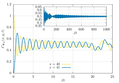
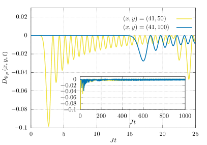
Figure 1: Time evolution of one-point function (left) and connected two-point function (right) of the total density operator $n_{x}$ after a quench from an initial state with Néel order in the particles (cf. (60)) in the thermodynamic limit (the insets report the long time behaviour). The one-point function relaxes to $1/2$ in the infinite-time limit while the connected two-point function goes to $\delta_{x,0}$. Note that at times $Jt=2x/4$ and $Jt=(x+y)/4$ the correlations begin to be affected by the boundary (the maximal velocity for the propagation of correlations is $v_{\rm max}=4J$).

We remark that Property 1 can also be used to compute more complicated functions of $\{n_{x}\}_{x=1}^{L}$. An interesting example is the time-evolution of the full counting statistics of

$$N_{A}=\sum_{y\in A}n_{y},$$ (66)

i.e., the total number of spinfull fermions in a given subsystem $A\subset\{1,\ldots,L\}$, on the time evolving state $e^{-\mathrm{i}tH_{\infty}}\ket{N}$. The full counting statistics of a certain observable $\mathcal{O}$ in a state $\ket{\Phi}$ is the probability distribution for the outcomes of measurements of $\mathcal{O}$ in $\ket{\Phi}$ and, as such, encodes detailed information about the quantum fluctuations $\mathcal{O}$. In particular, over the last few years there has been increasing interest in the time-evolution of full counting statistics after quantum quenches gritsev2006full ; kitagawa2011the ; eisler2013full ; lovas2017full ; groha2018full ; bastianello2018exact ; collura2020how .

The full counting statistics is completely specified by its Fourier transform, the characteristic function of the probability distribution, which in our case reads as

$$\chi_{\Psi}(t,A,\lambda)\equiv\braket{\Psi}{e^{\mathrm{i}tH_{\infty}}e^{i\lambda N_{A}}e^{-\mathrm{i}tH_{\infty}}}{\Psi}=\braket{\Psi_{f}}{e^{\mathrm{i}tH_{\rm tb}}e^{i\lambda D_{A}}e^{-\mathrm{i}tH_{\rm tb}}}{\Psi_{f}}\,,$$ (67)

where we again used Property 1 and we introduced

$$D_{A}=\sum_{y\in A}d_{y}.$$ (68)

The r.h.s. of (67) is immediately expressed as the determinant of a $|A|\times|A|$ matrix eisler2013full ; klich2003an ; klich2014a . In particular we have

$$\chi_{\Psi}(t,A,\lambda)=\det(I+(e^{i\lambda}-1){\mathbb{C}}^{\Psi_{f}}_{A}(t)),$$ (69)

where $I$ denotes the identity matrix and

$$[{\mathbb{C}}^{\Psi_{f}}_{A}(t)]_{x,y}=\braket{\Psi_{f}}{e^{\mathrm{i}tH_{\rm tb}}f_{x}^{\dagger}f_{y}^{\phantom{{\dagger}}}e^{-\mathrm{i}tH_{\rm tb}}}{\Psi_{f}}\,,\qquad x,y=1,\ldots,|A|\,.$$ (70)

is the correlation matrix reduced to the subsystem $A$. In particular, for a state with Néel order in the particles (cf. (60)) we have

$$[{\mathbb{C}}^{{N_{f}}}_{A}(t)]_{x,y}=\delta_{x,y}+\frac{(-1)^{y}}{L+1}\sum_{k}\sin(kx)\sin(ky)e^{-4iJ\cos(k)t}$$ (71)

where we introduced

$$\ket{N_{f}}=\prod_{x=0}^{L/2-1}f^{\dagger}_{2x+1}\ket{\fullmoon}\,.$$ (72)

Specifically, in the thermodynamic limit we find

$${\textstyle\lim_{\rm th}}[{\mathbb{C}}^{{N_{f}}}_{A}(t)]_{x,y}=\delta_{x,y}-\frac{i^{x+y}}{2}(J_{x-y}(4Jt)-(-1)^{x}J_{x+y}(4Jt))\,,\qquad x,y=1,\ldots,|A|\,.$$ (73)

The time evolution of the characteristic function (67) for two different values of $\lambda$ is depicted in Fig. 2. We see that the Néel order melts very rapidly after the quench.

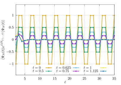
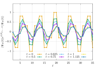
Figure 2: Characteristic function $\chi_{N}(t,A,\lambda)$ (cf. (67)) vs subsystem size for different times after a quench from the state (60) in the thermodynamic limit. The two panels correspond to $\lambda=\pi$ (left) and $\lambda=7\pi/5$ (right). In both cases $\chi_{N}(t,A,\lambda)$ approaches 0 for all $\ell$ for large times, signalling the melting of the order.

Before concluding this subsection we note that Property 1 can be immediately extended to initial states of the form

$$\ket{\Psi^{(g)}}=\left[\sum_{\{y_{j}\},\{s_{j}\}}A_{\{y_{j}\},\{s_{j}\}}\prod_{j=1}^{N}c^{\dagger}_{y_{j},\sigma_{j}}\right]\ket{0}\!,$$ (74)

where $|\{y_{j}\}|\!=\!|\{s_{j}\}|\!=\!N\!<\!L$. In this case, using that $d_{x}$ acts diagonally on the spin sector we find

$$\braket{\Psi^{(g)}}{e^{\mathrm{i}tH_{\infty}}F(n_{x_{1}},\ldots,n_{x_{m}})e^{-\mathrm{i}tH_{\infty}}}{\Psi^{(g)}}=\sum_{\{y_{j}\},\{s_{j}\}}|A_{\{y_{j}\},\{s_{j}\}}|^{2}\braket{\Psi_{f\{y_{j}\}}}{e^{\mathrm{i}tH_{\rm tb}}F(d_{x_{1}},\ldots,d_{x_{m}})e^{-\mathrm{i}tH_{\rm tb}}}{\Psi_{f\{y_{j}\}}}\!,$$ (75)

where, for the sake of clarity, we reported the explicit dependence of the state (52) on the set of particle positions $\{y_{j}\}$.

IV.2 Two-point correlators

The second class of operators whose dynamics simplifies when evolving from the states (48) are

$$c^{(\dagger)}_{x,\uparrow(\downarrow)}c^{(\dagger)}_{y,\uparrow(\downarrow)},$$ (76)

i.e., quadratic monomials of spin-full operators. In particular, we consider the only two equal-time two point functions which are not identically vanishing because violating spin or particle number conservation, namely

$$C_{\uparrow,\Psi}(x,y,t)\equiv\braket{\Psi}{e^{\mathrm{i}t{H}_{\infty}}c^{\dagger}_{x,\uparrow}c^{\phantom{\dagger}}_{y,\uparrow}e^{-\mathrm{i}t{H}_{\infty}}}{\Psi},$$ (77)

$$C_{\downarrow,\Psi}(x,y,t)\equiv\braket{\Psi}{e^{\mathrm{i}t{H}_{\infty}}c^{\dagger}_{x,\downarrow}c^{\phantom{\dagger}}_{y,\downarrow}e^{-\mathrm{i}t{H}_{\infty}}}{\Psi}.$$ (78)

Firstly, we use a simple argument to rewrite the second correlator as the expectation of the operator with both spins up, with respect to a spin-flipped state. Let $\mathcal{F}$ be the unitary spin-flip operator such that

$$\mathcal{F}c^{\left(\dagger\right)}_{x,\uparrow}\mathcal{F}^{\dagger}=c^{\left(\dagger\right)}_{x,\downarrow},\qquad\mathcal{F}c^{\left(\dagger\right)}_{x,\downarrow}\mathcal{F}^{\dagger}=c^{\left(\dagger\right)}_{x,\uparrow}\,.$$ (79)

Inserting this operator into the correlator gives

$$C_{\downarrow,\Psi}(x,y,t)=\braket{\Psi}{\mathcal{F}^{\dagger}\mathcal{F}e^{\mathrm{i}t{H}_{\infty}}\mathcal{F}^{\dagger}\mathcal{F}c^{\dagger}_{x,\downarrow}\mathcal{F}^{\dagger}\mathcal{F}c^{\phantom{\dagger}}_{y,\downarrow}\mathcal{F}^{\dagger}\mathcal{F}e^{-\mathrm{i}t{H}_{\infty}}\mathcal{F}^{\dagger}\mathcal{F}}{\Psi}\,.$$ (80)

Noting that Hamiltonian (1) is invariant under this transformation, the expectation value can be rewritten as

$$C_{\downarrow,\Psi}(x,y,t)=C_{\uparrow,\Psi^{\prime}}(x,y,t)\,,$$ (81)

where

$$\ket{\Psi^{\prime}}=\prod_{j=1}^{N}c^{\dagger}_{x_{j},\bar{\sigma}_{j}}\ket{0}\,,\qquad\bar{\uparrow}=\,\downarrow\,,\qquad\bar{\downarrow}=\,\uparrow\,.$$ (82)

Therefore, to calculate the correlators of interest, we will calculate the expectation value of the operator with both spins up, but with respect to a generic state $\ket{\Psi}$. This makes the calculation easier, as the Kumar mapping (9) is simpler on fermions with spin up.

Employing a similar reasoning we can also restrict ourselves to the case $\max(x,y)>L/2$, which, as we will see, is easier to treat with the unitary transformation (45). Indeed, if $\max(x,y)\leq L/2$ we can apply the unitary reflection operator $\mathcal{R}$ acting as

$$\mathcal{R}c^{\left(\dagger\right)}_{x,\uparrow}\mathcal{R}^{\dagger}=c^{\left(\dagger\right)}_{L+1-x,\uparrow},\qquad\mathcal{R}c^{\left(\dagger\right)}_{x,\downarrow}\mathcal{R}^{\dagger}=c^{\left(\dagger\right)}_{L+1-x,\downarrow}\,.$$ (83)

This gives

$$C_{\uparrow,\Psi}(x,y,t)=C_{\uparrow,\Psi^{\prime\prime}}(L+1-x,L+1-y,t),$$ (84)

with

$$\ket{\Psi^{\prime\prime}}=\prod_{j=1}^{N}c^{\dagger}_{L+1-x_{j},\sigma_{j}}\ket{0}\,.$$ (85)

Analogously

$$C_{\downarrow,\Psi}(x,y,t)=C_{\uparrow,\Psi^{\prime\prime\prime}}(L+1-x,L+1-y,t),$$ (86)

with

$$\ket{\Psi^{\prime\prime\prime}}=\prod_{j=0}^{N}c^{\dagger}_{L+1-x_{j},\bar{\sigma}_{j}}\ket{0}\,.$$ (87)

In summary, to evaluate $C_{\uparrow,\Psi}(x,y,t)$ and $C_{\downarrow,\Psi}(x,y,t)$ for all $x$ and $y$ here we consider

$$C_{\uparrow,\Psi}(x,y,t),\qquad\max(x,y)>L/2\,,$$ (88)

and access all the other cases by performing the appropriate spin-flip and reflections of the state. We begin our analysis of $C_{\uparrow,\Psi}(x,y,t)$: applying the Kumar mapping, the correlators are written as

$$C_{\uparrow,\Psi}(x,y,t)=\braket{\Psi}{e^{\mathrm{i}t{H}_{\infty}}(f^{\dagger}_{x}+(-1)^{x+1}f^{\phantom{\dagger}}_{x})(f^{\phantom{\dagger}}_{y}+(-1)^{y+1}f^{\dagger}_{y})\sigma_{+,x}\sigma_{-,y}e^{-\mathrm{i}t{H}_{\infty}}}{\Psi}\,,$$ (89)

where the Hamiltonian is given by (18). This can be further simplified using the fact that the initial state has fixed particle number

$$C_{\uparrow,\Psi}(x,y,t)=\braket{\Psi}{e^{\mathrm{i}t{H}_{\infty}}(f^{\dagger}_{x}f^{\phantom{\dagger}}_{y}+(-1)^{x+y}f_{x}f^{\dagger}_{y})\sigma_{+,x}\sigma_{-,y}e^{-\mathrm{i}t{H}_{\infty}}}{\Psi}\,.$$ (90)

To write the infinite interaction Hamiltonian as the free Hamiltonian $H_{\rm tb}$ (42) in the spinless fermions, we next apply the unitary transformation (32)

$$C_{\uparrow,\Psi}(x,y,t) =\braket{\Psi}{\mathcal{U}\mathcal{U}^{\dagger}e^{\mathrm{i}t{H}_{\infty}}\mathcal{U}\mathcal{U}^{\dagger}(f^{\dagger}_{x}f^{\phantom{\dagger}}_{y}+(-1)^{x+y}f^{\phantom{\dagger}}_{x}f^{\dagger}_{y})\sigma_{+,x}\sigma_{-,y}\mathcal{U}\mathcal{U}^{\dagger}e^{-\mathrm{i}t{H}_{\infty}}\mathcal{U}\mathcal{U}^{\dagger}}{\Psi}$$ (91)

$$=\bra{\Psi_{f}}\bra{\Psi_{s}}e^{\mathrm{i}tH_{\rm tb}}\mathcal{U}^{\dagger}(f^{\dagger}_{x}f^{\phantom{\dagger}}_{y}+(-1)^{x+y}f^{\phantom{\dagger}}_{x}f^{\dagger}_{y})\sigma_{+,x}\sigma_{-,y}\mathcal{U}e^{-\mathrm{i}tH_{\rm tb}}\ket{\Psi_{f}}\ket{\Psi_{s}}\,,$$ (92)

where we used

$$\mathcal{U}^{\dagger}\ket{\Psi}=\ket{\Psi_{f}}\ket{\Psi_{s}},$$ (93)

with

$$\ket{\Psi_{f}}=\prod_{j=1}^{N}f^{\dagger}_{x_{j}},\qquad\qquad\ket{\Psi_{s}}=\ket{\underbrace{\sigma_{N},\sigma_{N-1},\ldots,\sigma_{1}}_{N},\underbrace{-,\ldots,-}_{L-N}}.$$ (94)

The unitary operator $\mathcal{U}$ is a product of operators $U_{z}$, and those with $z=1,2,\ldots,\min(x,y)-1$ can be commuted left through the spins and spinless fermions, cancelling with their counterparts in the operator $\mathcal{U}^{\dagger}$. This leaves

$$C_{\uparrow,\Psi}(x,y,t)=\bra{\Psi_{f}}\bra{\Psi_{s}}e^{\mathrm{i}tH_{\rm tb}}U^{\dagger}_{L}\cdots U^{\dagger}_{\min(x,y)}(f^{\dagger}_{x}f^{\phantom{\dagger}}_{y}+(-1)^{x+y}f^{\phantom{\dagger}}_{x}f^{\dagger}_{y})\sigma_{+,x}\sigma_{-,y}U_{\min(x,y)}\cdots U_{L}e^{-\mathrm{i}tH_{\rm tb}}\ket{\Psi_{f}}\ket{\Psi_{s}}\,.$$ (95)

The operators $U_{z}$ act on the creation and annihilation operators in the fermions as follows

$$U^{(\dagger)}_{z}f^{\dagger}_{z}=\mathcal{X}^{(\dagger)}_{z},\qquad U^{(\dagger)}_{z}f^{\phantom{\dagger}}_{z}=I\,.$$ (96)

Therefore, first and last terms in the product can be simplified, by multiplying them by the fermions at sites $x$ and $y$ resulting in

$$C_{\uparrow,\Psi}(x,y,t)= \bra{\Psi_{t}}T_{\leftarrow}\left[\mathcal{X}^{\dagger}_{x}\prod_{z=\min(x,y)+1}^{\max(x,y)-1}U^{\dagger}_{z}\right]f^{\dagger}_{x}f^{\phantom{\dagger}}_{y}\sigma_{+,x}\sigma_{-,y}T_{\rightarrow}\left[\mathcal{X}_{y}\prod_{z=\min(x,y)+1}^{\max(x,y)-1}U^{\dagger}_{z}\right]\ket{\Psi_{t}}$$

$$+(-1)^{x+y}\bra{\Psi_{t}}T_{\leftarrow}\left[\mathcal{X}^{\dagger}_{y}\prod_{z=\min(x,y)+1}^{\max(x,y)-1}U^{\dagger}_{z}\right]f^{\phantom{\dagger}}_{x}f^{{\dagger}}_{y}\sigma_{+,x}\sigma_{-,y}T_{\rightarrow}\left[\mathcal{X}_{x}\prod_{z=\min(x,y)+1}^{\max(x,y)-1}U^{\dagger}_{z}\right]\ket{\Psi_{t}}\,,$$ (97)

Here, to write this expression in compact form we introduced the following $z$-ordered products of non-commuting operators

$$T_{\leftarrow}\left[O_{x}O^{\prime}_{y}\right]=\begin{cases}O_{x}O^{\prime}_{y}&x>y\\ O^{\prime}_{y}O_{x}&x<y\end{cases},\qquad T_{\rightarrow}\left[O_{x}O^{\prime}_{y}\right]=\begin{cases}O^{\prime}_{y}O_{x}&x>y\\ O_{x}O^{\prime}_{y}&x<y\end{cases},$$ (98)

the state

$$\ket{\Psi_{t}}\equiv U_{\max(x,y)+1}\cdots U_{L}e^{-\mathrm{i}tH_{\rm tb}}\ket{\Psi_{f}}\ket{\Psi_{s}},$$ (99)

and used the convention

$$\prod_{z=a}^{b}U^{\dagger}_{z}=I,\qquad\text{for}\qquad b<a\,.$$ (100)

To evaluate (97), we will next expand the operators $U_{x}$ which will then allow us to write each term as a product of a correlator in just the spinless fermions (depending on time) and a correlator in just the spins (independent of time). To express this succinctly we introduce the following set of projectors

$$\mathcal{P}_{x}^{(k)}\equiv\begin{cases}1-d_{x},&k=0\\ d_{x},&k=1\end{cases}\,.$$ (101)

In this succinct notation, the operators $U_{x}$ can be written as

$$U_{x}=\sum_{k=0,1}\mathcal{X}_{x}^{k}\mathcal{P}_{x}^{(k)}\,.$$ (102)

We can then write the two-point function as a linear combination of terms, where each term is the product of a correlator in the spinless fermions and a correlator in the spins. In particular we have

$$C_{\uparrow,\Psi}(x,y,t)= \!\!\!\sum_{\{k_{z}\}\in\{0,1\}}\mathcal{C}_{\Psi_{s}}(x,y,\{k_{z}\})\braket{\Psi_{f}}{e^{\mathrm{i}tH_{\rm tb}}f^{\dagger}_{x}f_{y}\prod_{\begin{subarray}{c}z=\min(x,y)+1\\ z\neq\max(x,y)\end{subarray}}^{L}\!\!\!\mathcal{P}^{(k_{z})}_{z}e^{-\mathrm{i}tH_{\rm tb}}}{\Psi_{f}}$$

$$+(-1)^{x+y}\!\!\!\sum_{\{k_{z}\}\in\{0,1\}}\!\!\!\!\!\mathcal{D}_{\Psi_{s}}(y,x,\{k_{z}\})\braket{\Psi_{f}}{e^{\mathrm{i}tH_{\rm tb}}f_{x}f_{y}^{\dagger}\prod_{\begin{subarray}{c}z=\min(x,y)+1\\ z\neq\max(x,y)\end{subarray}}^{L}\!\!\!\mathcal{P}^{(k_{z})}_{z}e^{-\mathrm{i}tH_{\rm tb}}}{\Psi_{f}},\qquad x\neq y,$$ (103)

$$C_{\uparrow,\Psi}(y,y,t)= \!\!\!\sum_{\{k_{z}\}\in\{0,1\}}\!\!\!\!\!\mathcal{E}_{\Psi_{s}}(y,\{k_{z}\})\braket{\Psi_{f}}{e^{\mathrm{i}tH_{\rm tb}}\prod_{z=y}^{L}\mathcal{P}^{(k_{z})}_{z}e^{-\mathrm{i}tH_{\rm tb}}}{\Psi_{f}}.$$ (104)

To write these expressions we used

$$\mathcal{P}_{x}^{(k)}\mathcal{P}_{x}^{(p)}=\mathcal{P}_{x}^{(k)}\delta_{p,k},$$ (105)

and defined

$$\mathcal{C}_{\Psi_{s}}(x,y,\{k_{z}\}) \equiv\begin{cases}\bra{\Psi_{s,k_{x+1},\ldots,k_{L}}}\mathcal{X}^{-1}_{x}\sigma_{+,x}\mathcal{X}_{x-1}^{-k_{x-1}}\cdots\mathcal{X}_{y+1}^{-k_{y+1}}\sigma_{-,y}\mathcal{X}_{y}\mathcal{X}_{y+1}^{k_{y+1}}\cdots\mathcal{X}_{x-1}^{k_{x-1}}\ket{\Psi_{s,k_{x+1},\ldots,k_{L}}}&x>y\\ \\ \bra{\Psi_{s,k_{y+1},\ldots,k_{L}}}\mathcal{X}_{y-1}^{-k_{y-1}}\cdots\mathcal{X}_{x+1}^{-k_{x+1}}\mathcal{X}^{-1}_{x}\sigma_{+,x}\mathcal{X}_{x+1}^{k_{x+1}}\cdots\mathcal{X}_{y-1}^{k_{y-1}}\sigma_{-,y}\mathcal{X}_{y}\ket{\Psi_{s,k_{y+1},\ldots,k_{L}}}&x<y\\ \end{cases},$$ (106)

$$\mathcal{D}_{\Psi_{s}}(x,y,\{k_{z}\}) \equiv\begin{cases}\bra{\Psi_{s,k_{x+1},\ldots,k_{L}}}\mathcal{X}_{x-1}^{-k_{x-1}}\cdots\mathcal{X}_{y+1}^{-k_{y+1}}\mathcal{X}^{-1}_{y}\sigma_{-,y}\mathcal{X}_{y+1}^{k_{y+1}}\cdots\mathcal{X}_{x-1}^{k_{x-1}}\sigma_{+,x}\mathcal{X}_{x}\ket{\Psi_{s,k_{x+1},\ldots,k_{L}}}&x>y\\ \\ \bra{\Psi_{s,k_{y+1},\ldots,k_{L}}}\mathcal{X}_{y}^{-1}\sigma_{-,y}\mathcal{X}_{y-1}^{-k_{y-1}}\cdots\mathcal{X}_{x+1}^{-k_{x+1}}\sigma_{+,x}\mathcal{X}_{x}\mathcal{X}_{x+1}^{k_{x+1}}\cdots\mathcal{X}_{y-1}^{k_{y-1}}\ket{\Psi_{s,k_{y+1},\ldots,k_{L}}}&x<y\\ \end{cases},$$ (107)

$$\mathcal{E}_{\Psi_{s}}(y,\{k_{z}\}) \equiv\braket{\Psi_{s,k_{y},\ldots,k_{L}}}{\sigma_{+,y}\sigma_{-,y}}{\Psi_{s,k_{y},\ldots,k_{L}}},$$ (108)

with

$$\ket{\Psi_{s,k_{a},\ldots,k_{b}}}=\mathcal{X}_{a}^{k_{a}}\cdots\mathcal{X}_{b}^{k_{b}}\ket{\Psi_{s}}\,.$$ (109)

As shown in Appendix B, the above expressions can be written in the following drastically simpler form

$$\mathcal{C}_{\Psi_{s}}(x,y,\{k_{z}\}) =\braket{\Psi_{s}}{\mathcal{X}_{L}^{-K_{2}}[\mathcal{X}_{\max(x,y)}^{-K_{1}-1}[I_{\min(x,y)-1}\otimes P^{(1)}{y-x|+1,K_{1}}]\mathcal{X}_{{\max(x,y)}}^{K_{1}+1}]\!\otimes\!I_{L-\max(x,y)}\mathcal{X}_{L}^{K_{2}}|\Psi_{s}}{,}$$ (110)

$$\mathcal{D}_{\Psi_{s}}(x,y,\{k_{z}\}) =\braket{\Psi_{s}}{\mathcal{X}_{L}^{-K_{2}}[\mathcal{X}_{\max(x,y)}^{-K_{1}-1}[I_{\min(x,y)-1}\otimes P^{(2)}{y-x|+1,K_{1}}]\mathcal{X}_{{\max(x,y)}}^{K_{1}+1}]\!\otimes\!I_{L-\max(x,y)}\mathcal{X}_{L}^{K_{2}}|\Psi_{s}}{,}$$ (111)

$$\mathcal{E}_{\Psi_{s}}(y,\{k_{z}\}) =\braket{\Psi_{s}}{\mathcal{X}_{L}^{-K_{2}}\mathcal{X}_{y}^{-k_{y}}\sigma_{+,y}\sigma_{-,y}\mathcal{X}_{y}^{k_{y}}\mathcal{X}_{L}^{K_{2}}}{\Psi_{s}},$$ (112)

where we introduced the rank-1 projectors

$$P^{(1)}_{a,b} =\ket{\underbrace{-\ldots-}_{a-b-1}\underbrace{+\ldots+}_{b+1}}\bra{\underbrace{-\ldots-}_{a-b-1}\underbrace{+\ldots+}_{b+1}}, a\geq b+1,$$ (113)

$$P^{(2)}_{a,b} =\ket{\underbrace{+\ldots+}_{a-b-1}\underbrace{-\ldots-}_{b+1}}\bra{\underbrace{+\ldots+}_{a-b-1}\underbrace{-\ldots-}_{b+1}}, a\geq b+1,$$ (114)

and we set

$$K_{1}\equiv\sum_{z=\min(x,y)+1}^{\max(x,y)-1}k_{z}\in\{0,\ldots,|y-x|-1\},\qquad K_{2}\equiv\!\!\!\!\!\sum_{z=\max(x,y)+1}^{L}\!\!\!\!\!k_{z}\in\{0,\ldots,L-\max(x,y)\}\,.$$ (115)

The expressions (103, 110, 111) and (104, 112) provide a substantial simplification in the calculation of correlation functions: since the correlators (110)–(112) are constant with respect to time, they can be evaluated once and for all and regarded as fixed coefficients. Given a set of coefficients $\{\mathcal{C}_{\Psi_{s}}(x,y,\{k_{z}\}),\mathcal{D}_{\Psi_{s}}(x,y,\{k_{z}\}),\mathcal{E}_{\Psi_{s}}(y,\{k_{z}\})\}$ one can then compute the time-evolution of $C_{\uparrow,\Psi}(x,y,t)$ by evaluating a number of correlators in the tight binding model evolving from a Fock state $\ket{\Psi_{f}}$. Since the latter states are Gaussian, this task can be performed efficiently by writing the free fermion correlators in terms of determinants. Although the sums in (103) and (104) generically involve a very large number of terms (of the order of $2^{L}$), for specific states (94) and positions $x$ and $y$ the sums can be exactly performed leading to explicit analytical expressions. For instance, let us consider two specific “generalised nested Néel” states of Ref. bertini2017quantum :

$$\ket{N_{22}} =\prod_{x=1}^{L/4}c^{\dagger}_{4x-2,\uparrow}c^{\dagger}_{4x,\downarrow}\ket{0}\,, \ket{N^{\prime}_{22}} =\prod_{x=1}^{L/4}c^{\dagger}_{4x-2,\downarrow}c^{\dagger}_{4x,\uparrow}\ket{0}\,,$$ (116a)

$$\ket{N^{\prime\prime}_{22}} =\prod_{x=0}^{L/4-1}c^{\dagger}_{4x+1,\downarrow}c^{\dagger}_{4x+3,\uparrow}\ket{0}\,, \ket{N^{\prime\prime\prime}_{22}} =\prod_{x=0}^{L/4-1}c^{\dagger}_{4x+1,\uparrow}c^{\dagger}_{4x+3,\downarrow}\ket{0}\,,$$ (116b)

and

$$\ket{N_{23}} =\prod_{x=1}^{L/6}c^{\dagger}_{6x-4,\uparrow}c^{\dagger}_{6x-2,\downarrow}c^{\dagger}_{6x,\downarrow}\ket{0}\,, \ket{N^{\prime}_{23}} =\prod_{x=1}^{L/6}c^{\dagger}_{6x-4,\downarrow}c^{\dagger}_{6x-2,\uparrow}c^{\dagger}_{6x,\uparrow}\ket{0}\,,$$ (117a)

$$\ket{N^{\prime\prime}_{23}} =\prod_{x=0}^{L/6-1}c^{\dagger}_{6x+1,\downarrow}c^{\dagger}_{6x+3,\downarrow}c^{\dagger}_{6x+5,\uparrow}\ket{0}\,, \ket{N^{\prime\prime\prime}_{23}} =\prod_{x=0}^{L/6-1}c^{\dagger}_{6x+1,\uparrow}c^{\dagger}_{6x+3,\uparrow}c^{\dagger}_{6x+5,\downarrow}\ket{0}\,.$$ (117b)

Note that in the case of (116) we took the chain length to be multiple of $4$ while in the case of (117) we took it to be a multiple of $6$. We also remark that the dynamics from the states (116) can also be studied with the approach of Ref. zhang2019quantum but the ones from (117) can not.

IV.2.1 States (116)

For the initial states (116) we find

$$\ket{N_{22f}}=\ket{N^{\prime}_{22f}}=\ket{N_{f}}\equiv\prod_{x=0}^{L/2-1}f^{\dagger}_{2x+1}\ket{\fullmoon}, \ket{N^{\prime\prime}_{22f}}=\ket{N^{\prime\prime\prime}_{22f}}=\ket{\bar{N}_{f}}\equiv\prod_{x=0}^{L/2-1}f^{\dagger}_{2x}\ket{\fullmoon},$$ (118)

$$\ket{N_{22s}}=\ket{N^{\prime\prime\prime}_{22s}}=\ket{S}\equiv\prod_{y=1}^{L/4}\sigma_{+,2y-1}\ket{-}\!, \ket{N_{22s}}=\ket{N^{\prime\prime\prime}_{22s}}=\ket{\bar{S}}\equiv\prod_{y=1}^{L/4}\sigma_{+,2y}\ket{-}\!.$$ (119)

From the expressions (118, 119) and the explicit form (110)–(112) of the coefficients one can deduce a number of general constrains. First we note that $\mathcal{C}(x,y,\{k_{z}\})$ and $\mathcal{D}(x,y,\{k_{z}\})$ respectively vanish for $K_{1}>1$ and $|x-y|-K_{1}<2$ because the states (119) do not feature a block of up spins of size larger than one. The second observation is that all coefficients vanish if $|x-y|>L/2$. This is because the projectors (113) and (114) can give a non-zero result only if the blocks of down spins in (113)–(114) are contracted with the block of down spins in the states (119). This can happen only if the size of the block of down spins in the states is larger then or equal to the support of the projectors. Noting that the former is $L/2+1$ and the latter $|x-y|+1$ gives the above inequality. Note that this constraint is in agreement with physical intuition: the correlations

$$C_{\uparrow,N_{22}}(x,y,t),\quad C_{\uparrow,N^{\prime}_{22}}(x,y,t),\quad C_{\uparrow,N^{\prime\prime}_{22}}(x,y,t),\quad C_{\uparrow,N^{\prime\prime\prime}_{22}}(x,y,t),$$ (120)

can be non zero only if there are no particles between $x$ and $y$. The best case is then when all other particles are squeezed at the two edges of the system leaving a free region of size $L/2$.

In fact, from (110)–(112) one can easily evaluate the coefficients explicitly. Here, however, we do not present the explicit expressions but rather show two simple examples where the correlations take a particularly simple form.

Number operators. The case $x=y$ is perhaps the simplest limiting case. Indeed, recalling the form (119) of the states, we immediately find

$$\mathcal{E}_{S}(y,\{k_{z}\})= \,\,\delta_{k_{y},1}{\rm mod}(K_{2},2)\theta(L/2\geq K_{2}+1)+\delta_{k_{y},0}{\rm mod}(K_{2}+y-1,2)\theta(L/2\geq K_{2}+y)\,,$$ (121)

$$\mathcal{E}_{\bar{S}}(y,\{k_{z}\})= \,\,\delta_{k_{y},1}{\rm mod}(K_{2}+1,2)\theta(L/2>K_{2}+1)+\delta_{k_{y},0}{\rm mod}(K_{2}+y,2)\theta(L/2>K_{2}+y)\,.$$ (122)

where we used $0\leq K_{2}\leq L-y$ (cf. (115)). Using now $y>L/2$ we find

$$\mathcal{E}_{S}(y,\{k_{z}\})= \,\,\delta_{k_{y},1}{\rm mod}(K_{2},2), \mathcal{E}_{\bar{S}}(y,\{k_{z}\})= \,\,\delta_{k_{y},1}{\rm mod}(K_{2}+1,2)\,.$$ (123)

Plugging back into (104) and using

$$\sum_{\{k_{z}\}\in\{0,1\}}{\rm mod}(k_{y+1}+\cdots+k_{L}+a,2)=\frac{1}{2}\sum_{\eta=\pm}\sum_{\{k_{z}\}\in\{0,1\}}\eta^{k_{y+1}+....+k_{L}+a+1},$$ (124)

we find

$$C_{\uparrow,N_{22}}(y,y,t) =\frac{1}{2}\braket{N_{f}}{e^{\mathrm{i}tH_{\rm tb}}d_{y}e^{-\mathrm{i}tH_{\rm tb}}}{N_{f}}-\frac{1}{2}\braket{N_{f}}{e^{\mathrm{i}tH_{\rm tb}}d_{y}\prod_{z=y+1}^{L}(1-2d_{z})e^{-\mathrm{i}tH_{\rm tb}}}{N_{f}},$$ (125)

$$C_{\uparrow,N^{\prime}_{22}}(y,y,t) =\frac{1}{2}\braket{N_{f}}{e^{\mathrm{i}tH_{\rm tb}}d_{y}e^{-\mathrm{i}tH_{\rm tb}}}{N_{f}}+\frac{1}{2}\braket{N_{f}}{e^{\mathrm{i}tH_{\rm tb}}d_{y}\prod_{z=y+1}^{L}(1-2n_{z})e^{-\mathrm{i}tH_{\rm tb}}}{N_{f}},$$ (126)

$$C_{\uparrow,N^{\prime\prime}_{22}}(y,y,t) =\frac{1}{2}\braket{\bar{N}_{f}}{e^{\mathrm{i}tH_{\rm tb}}d_{y}e^{-\mathrm{i}tH_{\rm tb}}}{\bar{N}_{f}}+\frac{1}{2}\braket{\bar{N}_{f}}{e^{\mathrm{i}tH_{\rm tb}}d_{y}\prod_{z=y+1}^{L}(1-2d_{z})e^{-\mathrm{i}tH_{\rm tb}}}{\bar{N}_{f}}$$

$$=\frac{1}{2}\braket{N_{f}}{e^{\mathrm{i}tH_{\rm tb}}d_{L+1-y}e^{-\mathrm{i}tH_{\rm tb}}}{N_{f}}+\frac{1}{2}\braket{N_{f}}{e^{\mathrm{i}tH_{\rm tb}}d_{L+1-y}\prod_{z=1}^{L-y}(1-2d_{z})e^{-\mathrm{i}tH_{\rm tb}}}{N_{f}},$$ (127)

$$C_{\uparrow,N^{\prime\prime\prime}_{22}}(y,y,t) =\frac{1}{2}\braket{\bar{N}_{f}}{e^{\mathrm{i}tH_{\rm tb}}d_{y}e^{-\mathrm{i}tH_{\rm tb}}}{\bar{N}_{f}}-\frac{1}{2}\braket{\bar{N}_{f}}{e^{\mathrm{i}tH_{\rm tb}}d_{y}\prod_{z=y+1}^{L}(1-2d_{z})e^{-\mathrm{i}tH_{\rm tb}}}{\bar{N}_{f}}$$

$$=\frac{1}{2}\braket{N_{f}}{e^{\mathrm{i}tH_{\rm tb}}d_{L+1-y}e^{-\mathrm{i}tH_{\rm tb}}}{N_{f}}-\frac{1}{2}\braket{N_{f}}{e^{\mathrm{i}tH_{\rm tb}}d_{L+1-y}\prod_{z=1}^{L-y}(1-2d_{z})e^{-\mathrm{i}tH_{\rm tb}}}{N_{f}},$$ (128)

where in the second lines of (127) and (128) we performed a reflection in the tight-binding model. Using (81), (84) and (86) we then have

$$C_{\uparrow/\downarrow,N_{22}}(y,y,t)=\frac{1}{2}\begin{cases}\displaystyle\braket{N_{f}}{e^{\mathrm{i}tH_{\rm tb}}d_{y}e^{-\mathrm{i}tH_{\rm tb}}}{N_{f}}\mp\braket{N_{f}}{e^{\mathrm{i}tH_{\rm tb}}d_{y}\prod_{z=y+1}^{L}\!\!(1-2d_{z})e^{-\mathrm{i}tH_{\rm tb}}}{N_{f}},&y>L/2\\ \\ \displaystyle\braket{N_{f}}{e^{\mathrm{i}tH_{\rm tb}}d_{y}e^{-\mathrm{i}tH_{\rm tb}}}{N_{f}}\pm\braket{N_{f}}{e^{\mathrm{i}tH_{\rm tb}}d_{y}\prod_{z=1}^{y-1}(1-2d_{z})e^{-\mathrm{i}tH_{\rm tb}}}{N_{f}},&y\leq L/2\end{cases}\,.$$ (129)

Finally, noting that

$$\ket{N_{f}}=e^{i\pi D_{\{1,\ldots,L\}}}\ket{N_{f}}=e^{i\pi L}\ket{N_{f}},\qquad[H_{\rm tb},D_{\{1,\ldots,L\}}]=0,$$ (130)

where $D_{A}$ is defined in (68), we can rewrite the expressions in the following compact form

$$C_{\uparrow/\downarrow,N_{22}}(y,y,t) =\frac{1}{2}\braket{N_{f}}{e^{\mathrm{i}tH_{\rm tb}}d_{y}(1\pm e^{i\pi D_{\{1,\ldots,y-1\}}})e^{-\mathrm{i}tH_{\rm tb}}}{N_{f}}$$

$$=\frac{1}{2}\braket{N_{f}}{e^{\mathrm{i}tH_{\rm tb}}d_{y}e^{-\mathrm{i}tH_{\rm tb}}}{N_{f}}\mp\frac{1}{4}\braket{N_{f}}{e^{\mathrm{i}tH_{\rm tb}}(e^{i\pi D_{\{1,\ldots,y\}}}-e^{i\pi D_{\{1,\ldots,y-1\}}})e^{-\mathrm{i}tH_{\rm tb}}}{N_{f}}\,.$$ (131)

Using (67) and (69) we then have

$$C_{\uparrow/\downarrow,N_{22}}(y,y,t) =\frac{1}{2}\braket{N_{f}}{d_{y}(t)}{N_{f}}\mp\frac{1}{4}(\chi_{N}(t,\{1,\ldots,y\},\pi)-\chi_{N}(t,\{1,\ldots,y-1\},\pi))$$

$$=\frac{1}{2}\braket{N_{f}}{d_{y}(t)}{N_{f}}\mp\frac{1}{4}\left(\det(\mathbb{I}-2{\mathbb{C}}^{N_{f}}_{\{1,\ldots,y\}}(t))-\det(\mathbb{I}-2{\mathbb{C}}^{N_{f}}_{\{1,\ldots,y-1\}}(t)\right)\,,$$ (132)

where the correlation matrix is reported explicitly in (70). Since the characteristic function $\chi_{N}(t,A,\lambda)$ decays very rapidly zero after a quench from a state with Néel ordering in the particles (cf. Fig 2), we expect $C_{\uparrow/\downarrow,N_{22}}(y,y,t)$ to rapidly approach $\braket{N_{f}}{d_{y}(t)}{N_{f}}/2$. This is explicitly demonstrated in Fig. 3.

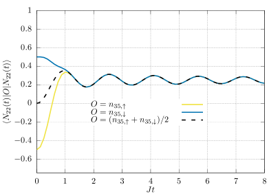
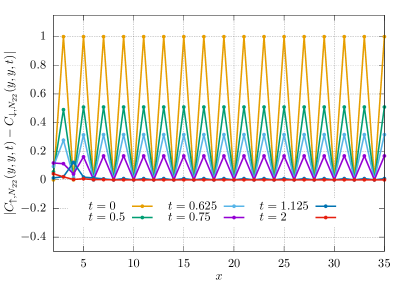
Figure 3: Dynamics of the number operators after a quench from the generalised nested Néel state (116) in the thermodynamic limit. The left panel shows the time evolution of the densities at $x=35$, comparing $C_{\uparrow,N_{22}}(y,y,t)$, $C_{\downarrow,N_{22}}(y,y,t)$, and $(C_{\uparrow,N_{22}}(y,y,t)+C_{\downarrow,N_{22}}(y,y,t))/2=\braket{N_{f}}{d_{y}(t)}{N_{f}}/2$. The right panel shows fixed-time slices of $|C_{\uparrow,N_{22}}(y,y,t)-C_{\downarrow,N_{22}}(y,y,t)|$.

Boundary Correlations. Another simple limiting case for the states (119) is $y=L$. Indeed, in this case we have that the range of values that $K_{2}$ can take is shrunk to $K_{2}=0$ (cf. (115)). Moreover, we immediately see that

$$\mathcal{C}_{\Psi_{s}}(x,L,\{k_{z}\})=\delta_{K_{1},0}\delta_{(s)_{1},+}\theta(x>L/2),\qquad\mathcal{D}_{\Psi_{s}}(x,L,\{k_{z}\})=0,$$ (133)

where $(s)_{1}$ is the first spin of $\ket{\Psi_{s}}$ (one of the two states (119)). Plugging into (103) this leads to

$$C_{\uparrow,\Psi}(x,y,t)=\delta_{(s)_{1},+}\theta(L/2>|x-y|)\braket{\Psi_{f}}{e^{\mathrm{i}tH_{\rm tb}}f^{\dagger}_{x}\prod_{z=x+1}^{L-1}(1-d_{z})f_{L}e^{-\mathrm{i}tH_{\rm tb}}}{\Psi_{f}}\,.$$ (134)

Using again (81), (84) and (86) we finally obtain

$$C_{\uparrow,N_{22}}(x,1,t)=\theta(x<L/2+1)\braket{N_{f}}{e^{\mathrm{i}tH_{\rm tb}}f^{\dagger}_{x}\prod_{z=2}^{x-1}(1-d_{z})f_{1}e^{-\mathrm{i}tH_{\rm tb}}}{N_{f}}\,,$$ (135)

$$C_{\downarrow,N_{22}}(x,L,t)=\theta(x>L/2)\braket{N_{f}}{e^{\mathrm{i}tH_{\rm tb}}f^{\dagger}_{x}\prod_{z=x+1}^{L-1}(1-d_{z})f_{L}e^{-\mathrm{i}tH_{\rm tb}}}{N_{f}}\,,$$ (136)

$$C_{\uparrow,N_{22}}(x,L,t)=C_{\downarrow,N_{22}}(x,1,t)=0\,.$$ (137)

These expressions are again written in terms of determinants involving the correlation matrix (70). In particular, we have

$$C_{\uparrow,N_{22}}(x,1,t)=\theta(x<L/2+1)\det({\mathbb{C}}^{N_{f}\prime}_{\{1,\ldots,x-1\}}(t))\,, C_{\downarrow,N_{22}}(x,L,t)=\theta(x>L/2)\det({\mathbb{C}}^{N_{f}\prime\prime}_{\{x,\ldots,L-1\}}(t)),$$ (138)

where we defined

$$[{\mathbb{C}}^{N_{f}\prime}_{A}]_{x,y}=[{\mathbb{C}}^{N_{f}}_{A}]_{x+1,y}-\delta_{x+1,y}\,,\qquad\qquad[{\mathbb{C}}^{N_{f}\prime\prime}_{A}]_{x,y}=[{\mathbb{C}}^{N_{f}}_{A}]_{x,y+1}-\delta_{x,y+1}\,.$$ (139)

A representative example of the dynamics of $C_{\uparrow,N}(x,1,t)$ in the thermodynamic limit is reported in Fig. 4

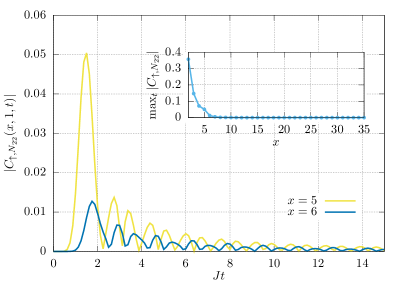
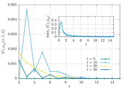
Figure 4: Dynamics of the bulk boundary correlation $C_{\uparrow,N_{22}}(x,1,t)$ after a quench from the nested Néel state (116) in the thermodynamic limit. The left panel reports the time evolution of $|C_{\uparrow,N_{22}}(x,1,t)|$ at two specific positions while the right panel shows four fixed-time cuts of $|C_{\uparrow,N_{22}}(x,1,t)|$ (the insets respectively show the decay in $x$ of $\max_{t}|C_{\uparrow,N_{22}}(x,1,t)|$ and in $t$ of $\max_{x}|C_{\uparrow,N_{22}}(x,1,t)|$).

IV.2.2 States (117)

For the states (117) we find

$$\ket{N_{23f}}=\ket{N^{\prime}_{23f}}=\ket{N_{f}}\equiv\prod_{x=0}^{L/2-1}f^{\dagger}_{2x+1}\ket{\fullmoon}, \ket{N^{\prime\prime}_{23f}}=\ket{N^{\prime\prime\prime}_{23f}}=\ket{\bar{N}_{f}}\equiv\prod_{x=0}^{L/2-1}f^{\dagger}_{2x}\ket{\fullmoon},$$ (140)

$$\ket{N_{23s}}=\ket{S_{1}}\equiv\prod_{y=1}^{L/6}\sigma_{+,3y}\ket{-}\!, \ket{N^{\prime}_{23s}}=\ket{S_{2}}\equiv\prod_{y=1}^{L/6}\sigma_{+,3y-2}\sigma_{+,3y-1}\ket{-}\!,$$ (141)

$$\ket{N^{\prime\prime}_{23s}}=\ket{\bar{S}_{1}}\equiv\prod_{y=1}^{L/6}\sigma_{+,3y-2}\ket{-}\!, \ket{N^{\prime\prime\prime}_{23s}}=\ket{\bar{S}_{2}}\equiv\prod_{y=0}^{L/6}\sigma_{+,3y-1}\sigma_{+,3y}\ket{-}.$$ (142)

Once again combining these expressions and the explicit forms (110)–(112) of the coefficients one can deduce a number of general constrains on $K_{1}$, $K_{2}$, $x$ and $y$. For instance, we have that all $\mathcal{C}$ coefficients vanish unless $K_{1}<3$ and all $\mathcal{D}$ coefficients vanish unless $|x-y|-K_{1}<4$. Finally, all coefficients are zero if $|x-y|>L/2+1$.

Focussing again on simple limiting cases, and using

$$\mathcal{E}_{S_{1}}(y,\{k_{z}\}) =\,\,\delta_{k_{y},1}\delta_{{\rm mod}(K_{2}+1,3)},$$ (143)

$$\mathcal{E}_{S_{2}}(y,\{k_{z}\}) =\,\,\delta_{k_{y},1}\delta_{{\rm mod}(K_{2},3)}+\delta_{k_{y},1}\delta_{{\rm mod}(K_{2}+2,3)}\,,$$ (144)

$$\mathcal{E}_{\bar{S}_{1}}(y,\{k_{z}\}) =\,\,\delta_{k_{y},1}\delta_{{\rm mod}(K_{2},3)},$$ (145)

$$\mathcal{E}_{\bar{S}_{2}}(y,\{k_{z}\}) =\,\,\delta_{k_{y},1}\delta_{{\rm mod}(K_{2}+1,3)}+\delta_{k_{y},1}\delta_{{\rm mod}(K_{2}+2,3)}\,,$$ (146)

for $y>L/2$, we find

$$C_{\uparrow,N_{23}}(y,y,t) =\frac{1}{3}\sum_{n=0}^{2}e^{i\frac{2\pi}{3}n}\braket{N_{f}}{e^{\mathrm{i}tH_{\rm tb}}d_{y}e^{i\frac{2\pi}{3}nD_{\{y+1,\ldots,L\}}}e^{-\mathrm{i}tH_{\rm tb}}}{N_{f}},$$ (147)

$$C_{\uparrow,N^{\prime}_{23}}(y,y,t) =\frac{1}{3}\sum_{n=0}^{2}(1+e^{i\frac{4\pi}{3}n})\braket{N_{f}}{e^{\mathrm{i}tH_{\rm tb}}d_{y}e^{i\frac{2\pi}{3}nD_{\{y+1,\ldots,L\}}}e^{-\mathrm{i}tH_{\rm tb}}}{N_{f}},$$ (148)

$$C_{\uparrow,N^{\prime\prime}_{23}}(y,y,t) =\frac{1}{3}\sum_{n=0}^{2}\braket{N_{f}}{e^{\mathrm{i}tH_{\rm tb}}d_{L-y+1}e^{i\frac{2\pi}{3}nD_{\{1,\ldots,L-y\}}}e^{-\mathrm{i}tH_{\rm tb}}}{N_{f}},$$ (149)

$$C_{\uparrow,N^{\prime\prime\prime}_{23}}(y,y,t) =\frac{1}{3}\sum_{n=0}^{2}(e^{i\frac{2\pi}{3}n}+e^{i\frac{4\pi}{3}n})\braket{N_{f}}{e^{\mathrm{i}tH_{\rm tb}}d_{L+1-y}e^{i\frac{2\pi}{3}nD_{\{1,\ldots,L-y\}}}e^{-\mathrm{i}tH_{\rm tb}}}{N_{f}}.$$ (150)

Employing now (81), (84) and (86) this leads to

$$C_{\uparrow,N_{23}}(y,y,t) =\frac{1}{3}\sum_{n=0}^{2}\braket{N_{f}}{e^{\mathrm{i}tH_{\rm tb}}d_{y}e^{i\frac{2\pi}{3}nD_{\{1,\ldots,y-1\}}}e^{-\mathrm{i}tH_{\rm tb}}}{N_{f}},$$

$$C_{\downarrow,N_{23}}(y,y,t) =\frac{1}{3}\sum_{n=0}^{2}(e^{i\frac{2\pi}{3}n}+e^{i\frac{4\pi}{3}n})\braket{N_{f}}{e^{\mathrm{i}tH_{\rm tb}}d_{y}e^{i\frac{2\pi}{3}nD_{\{1,\ldots,y-1\}}}e^{-\mathrm{i}tH_{\rm tb}}}{N_{f}}.$$ (151)

In terms of determinants we have

$$C_{\uparrow,N_{23}}(y,y,t) =\frac{1}{3}\braket{N_{f}}{e^{\mathrm{i}tH_{\rm tb}}d_{y}e^{-\mathrm{i}tH_{\rm tb}}}{N_{f}}$$

$$\quad+\frac{1}{3}\sum_{n=1}^{2}\frac{1}{e^{i\frac{2\pi}{3}n}-1}\left[\det(\mathbb{I}-(e^{i\frac{2\pi}{3}n}-1){\mathbb{C}}^{N_{f}}_{\{1,\ldots,y\}}(t))-\det(\mathbb{I}-(e^{i\frac{2\pi}{3}n}-1){\mathbb{C}}^{N_{f}}_{\{1,\ldots,y-1\}}(t)\right],$$

$$C_{\downarrow,N_{23}}(y,y,t) =\frac{2}{3}\braket{N_{f}}{e^{\mathrm{i}tH_{\rm tb}}d_{y}e^{-\mathrm{i}tH_{\rm tb}}}{N_{f}}$$

$$\quad+\frac{1}{3}\sum_{n=1}^{2}\frac{e^{i\frac{2\pi}{3}n}+e^{i\frac{4\pi}{3}n}}{e^{i\frac{2\pi}{3}n}-1}\left[\det(\mathbb{I}-(e^{i\frac{2\pi}{3}n}-1){\mathbb{C}}^{N_{f}}_{\{1,\ldots,y\}}(t))-\det(\mathbb{I}-(e^{i\frac{2\pi}{3}n}-1){\mathbb{C}}^{N_{f}}_{\{1,\ldots,y-1\}}(t)\right].$$ (152)

Moreover, using that the only non-zero coefficients for $y=L$ are

$$\mathcal{C}_{\bar{S}_{1}}(x,L,\{k_{z}\})=\delta_{K_{1},0}\theta(x>L/2),\qquad\mathcal{C}_{S_{2}}(x,L,\{k_{z}\})=(\delta_{K_{1},0}+\delta_{K_{1},1})\theta(x>L/2-1),$$ (153)

we find

$$C_{\uparrow,N_{23}}(x,1,t)=\theta(x<L/2+1)\det({\mathbb{C}}^{N_{f}\prime}_{\{1,\ldots,x-1\}}(t))\,,\,\,\,C_{\downarrow,N_{23}}(x,L,t)=\theta(x>L/2-1)\!\!\sum_{y=x+1}^{L-1}\!\!\!\det({\mathbb{C}}^{N_{f}\prime\prime}_{\{x,\ldots,L-1\},y}(t)),$$ (154)

where we defined

$$[{\mathbb{C}}^{N_{f}\prime\prime}_{A,y_{0}}]_{x,y}=\begin{cases}[{\mathbb{C}}^{N_{f}}_{A}]_{x,y+1}-\delta_{x,y+1}&x,y>y_{0}\\ [{\mathbb{C}}^{N_{f}}_{A}]_{x,y}-\delta_{x,y}&x>y_{0},\quad y\leq y_{0}\\ [{\mathbb{C}}^{N_{f}}_{A}]_{x-1,y+1}-\delta_{x-1,y+1}&y>y_{0},\quad x\leq y_{0}\\ [{\mathbb{C}}^{N_{f}}_{A}]_{x-1,y}-\delta_{x-1,y}&x,y\leq y_{0}\\ \end{cases}.$$ (155)

This treatment is easily generalised to all states $\ket{N_{pq}}$ with $p,q\geq 2$.

V Conclusions

In this paper we studied the real-time dynamics of the Hubbard model with open boundary conditions in the limit of infinite repulsion. In this limit, as shown in Ref. kumar2008exact , the Hamiltonian of the model can be unitarily mapped into the tight-binding model at the price of complicating the form of the observables. Here we showed that, in spite of this complication, one can efficiently compute the evolution of the expectation values of two classes of observables after a quench from initial states in product form. In particular, we pointed out that the expectation value of any function of the of the total density is exactly equal to the analogous quantity in the tight-binding model. Moreover, we proved that the two point functions of the Hubbard fermions can be expressed as linear combinations of determinants multiplied by simple time-independent coefficients, obtaining particularly simple expressions for the expectation value of the densities of particles of each separate species and for the correlation between one point at the boundary and one in the bulk evolving from the generalised nested Néel states of Ref. bertini2017quantum . Our results on the evolution of total densities are directly extended for initial states not in product form, while generic two point functions become more complicated when foregoing the product structure.

Our results are also the starting point for a number of interesting further developments. First we can use our results to study inhomogeneous initial states such as those corresponding to bipartitioning protocols with global spin imbalance. This would allow to obtain correlation functions which are not accessible in GHD (except for zero entropy states rcdd-20 ) potentially accessing the diffusive scale. Indeed, the strong coupling Hubbard can be thought of as a quantum version of the classical cellular automaton studied in Refs. medenjak2017diffusion ; klobas2018exactly , which could access the diffusion constant exactly. Another more difficult development concerns the use of our results as a starting point to set up an equations-of-motion scheme — similar to the one used to study prethermalization weakly interacting systems mk-08 ; EsslerPRB14 ; BEGR:PRL ; BEGR:PRB ; bc-20 — to study the Hubbard model with large but finite interaction. A final extension of our calculations, motivated by recent cold-atom experiments Fallani:tunablespin and by the results of Ref. zhang2019quantum , is to apply the generalised Kumar’s mapping of Ref. kumar2008canonical to the quench dynamics of a multispecies Hubbard model with SU(N) symmetry.

VI Acknowledgements

We thank Fabian Essler and Lev Vidmar for helpful discussions. BB was supported by the Royal Society through the University Research Fellowship No. 201102. BB thanks the University of Ljubljana for hospitality during the final stages of this project.

Appendix A Kumar mapping on the Hubbard Hamiltonian with finite interaction

To apply the Kumar mapping (9) to the Hamiltonian (1) we break sum across odd and even sites and then write everything in terms of the Majorana fermions

$${H}= -J\!\!\sum_{\alpha=\uparrow,\downarrow}\!\!\left[\sum_{x=1}^{L/2}\left(c^{\dagger}_{2x-1,\alpha}c_{2x,\alpha}+c^{\dagger}_{2x,\alpha}c_{2x-1,\alpha}\right)+\sum_{x=1}^{(L-1)/2}\left(c^{\dagger}_{2x,\alpha}c_{2x+1,\alpha}+c^{\dagger}_{2x+1,\alpha}c_{2x,\alpha}\right)\right]\!\!+U\sum_{x=1}^{L}\left(n_{x,\uparrow}-\frac{1}{2}\right)\left(n_{x,\downarrow}-\frac{1}{2}\right)$$

$$= -J\left[\sum_{x=1}^{L/2}\left(c^{\dagger}_{2x-1,\uparrow}c_{2x,\uparrow}+c^{\dagger}_{2x,\uparrow}c_{2x-1,\uparrow}\right)+\sum_{x=1}^{(L-1)/2}\left(c^{\dagger}_{2x,\uparrow}c_{2x+1,\uparrow}+c^{\dagger}_{2x+1,\uparrow}c_{2x,\uparrow}\right)\right.$$

$$+\left.\sum_{x=1}^{L/2}\left(c^{\dagger}_{2x-1,\downarrow}c_{2x,\downarrow}+c^{\dagger}_{2x,\downarrow}c_{2x-1,\downarrow}\right)+\sum_{x=1}^{(L-1)/2}\left(c^{\dagger}_{2x,\downarrow}c_{2x+1,\downarrow}+c^{\dagger}_{2x+1,\downarrow}c_{2x,\downarrow}\right)\right]\!\!+U\sum_{x=1}^{L}\left(n_{x,\uparrow}-\frac{1}{2}\right)\left(n_{x,\downarrow}-\frac{1}{2}\right)$$

$$= -J\left[\sum_{x=1}^{L/2}\left(a^{x}_{2x-1}\sigma_{2x-1}^{+}(-\mathrm{i}a^{y}_{2x}\sigma^{-}_{2x})+\mathrm{i}a^{y}_{2x}\sigma^{+}_{2x}a^{x}_{2x-1}\sigma^{-}_{2x-1}\right)+\sum_{x=1}^{(L-1)/2}\left(\mathrm{i}a^{y}_{2x}\sigma_{2x}^{+}a^{x}_{2x+1}\sigma^{-}_{2x+1}+a^{x}_{2x+1}\sigma^{+}_{2x+1}(-\mathrm{i}a^{y}_{2x}\sigma^{-}_{2x}\right)\right.$$

$$+\left.\sum_{x=1}^{L/2}\left(\tfrac{1}{2}(\mathrm{i}a^{y}_{2x-1}-a^{x}_{2x-1}\sigma^{z}_{2x-1})\tfrac{1}{2}(a^{x}_{2x}+\mathrm{i}a^{y}_{2x}\sigma^{z}_{2x})+\tfrac{1}{2}(a^{x}_{2x}-\mathrm{i}a^{y}_{2x}\sigma^{z}_{2x})\tfrac{1}{2}(-\mathrm{i}a^{y}_{2x-1}-a^{x}_{2x-1}\sigma^{z}_{2x-1})\right)\right.$$

$$\left.+\frac{1}{4}\sum_{x=1}^{(L-1)/2}\!\!\!\!\!\!\left((a^{x}_{2x}-\mathrm{i}a^{y}_{2x}\sigma^{z}_{2x})(-\mathrm{i}a^{y}_{2x+1}-a^{x}_{2x+1}\sigma^{z}_{2x+1})+(\mathrm{i}a^{y}_{2x+1}-a^{x}_{2x+1}\sigma^{z}_{2x+1})(a^{x}_{2x}+\mathrm{i}a^{y}_{2x}\sigma^{z}_{2x})\right)\right]\!\!$$

$$+\frac{U}{2}\sum_{x=1}^{L}\left(\frac{1}{2}-d_{x}\right).$$ (156)

Note that in the $U$-dependent term we have applied the identity (16). We then expand and simplify the summands of the first two sums, before combining them with the second two sums. This results in

$${H}= -J\left[\sum_{x=1}^{L/2}\left(a^{x}_{2x-1}\sigma_{2x-1}^{+}(-\mathrm{i}a^{y}_{2x}\sigma^{-}_{2x})+\mathrm{i}a^{y}_{2x}\sigma^{+}_{2x}a^{x}_{2x-1}\sigma^{-}_{2x-1}\right)+\sum_{x=1}^{(L-1)/2}\left(\mathrm{i}a^{y}_{2x}\sigma_{2x}^{+}a^{x}_{2x+1}\sigma^{-}_{2x+1}+a^{x}_{2x+1}\sigma^{+}_{2x+1}(-\mathrm{i}a^{y}_{2x}\sigma^{-}_{2x}\right)\right.$$

$$\left.+\frac{1}{4}\sum_{x=1}^{L/2}\left((\mathrm{i}a^{y}_{2x-1}-a^{x}_{2x-1}\sigma^{z}_{2x-1})(a^{x}_{2x}+\mathrm{i}a^{y}_{2x}\sigma^{z}_{2x})+(\mathrm{i}a^{y}_{2x-1}+a^{x}_{2x-1}\sigma^{z}_{2x-1})(a^{x}_{2x}-\mathrm{i}a^{y}_{2x}\sigma^{z}_{2x})\right)\right.$$

$$\left.+\frac{1}{4}\sum_{x=1}^{(L-1)/2}\left((\mathrm{i}a^{y}_{2x+1}+a^{x}_{2x+1}\sigma^{z}_{2x+1})(a^{x}_{2x}-\mathrm{i}a^{y}_{2x}\sigma^{z}_{2x})+(\mathrm{i}a^{y}_{2x+1}-a^{x}_{2x+1}\sigma^{z}_{2x+1})(a^{x}_{2x}+\mathrm{i}a^{y}_{2x}\sigma^{z}_{2x})\right)\right]\!\!$$

$$+\frac{U}{2}\sum_{x=1}^{L}\left(\frac{1}{2}-d_{x}\right)$$

$$= -\frac{J}{2}\left[\sum_{x=1}^{L/2}\left(2a^{x}_{2x-1}\sigma_{2x-1}^{+}(-\mathrm{i}a^{y}_{2x}\sigma^{-}_{2x})+2\mathrm{i}a^{y}_{2x}\sigma^{+}_{2x}a^{x}_{2x-1}\sigma^{-}_{2x-1}+\mathrm{i}a^{y}_{2x-1}a^{x}_{2x}-a^{x}_{2x-1}\sigma^{z}_{2x-1}\mathrm{i}a^{y}_{2x}\sigma^{z}_{2x}\right)\right.$$

$$+\left.\sum_{x=1}^{(L-1)/2}\left(2\mathrm{i}a^{y}_{2x}\sigma_{2x}^{+}a^{x}_{2x+1}\sigma^{-}_{2x+1}+2a^{x}_{2x+1}\sigma^{+}_{2x+1}(-\mathrm{i}a^{y}_{2x}\sigma^{-}_{2x})+\mathrm{i}a^{y}_{2x+1}a^{x}_{2x}-a^{x}_{2x+1}\sigma^{z}_{2x+1}\mathrm{i}a^{y}_{2x}\sigma^{z}_{2x}\right)\right]\!\!$$

$$+\frac{U}{2}\sum_{x=1}^{L}\left(\frac{1}{2}-d_{x}\right).$$

The two $J$-dependent sums have the same form, so we combine them introducing a sum over $s=\pm 1$. Note that from the boundary conditions $a^{x}_{L+1}=a^{y}_{L+1}=0$, so the term with $x=L/2,\ s=1$ contributes nothing to the sum. The summand has a common factor in the Majorana fermions, so we extract this and simplify the part depending on the spins

$${H} =-\frac{J}{2}\sum_{s=\pm 1}\sum_{x=1}^{L/2}\left[\mathrm{i}a^{y}_{2x}a^{x}_{2x+s}\left(2\sigma_{2x+s}^{+}\sigma^{-}_{2x}+2\sigma^{+}_{2x}\sigma^{-}_{2x+s}+\sigma^{z}_{2x+s}\sigma^{z}_{2x}\right)+\mathrm{i}a^{y}_{2x+s}a^{x}_{2x}\right]\!+\frac{U}{2}\sum_{x=1}^{L}\left(\frac{1}{2}-d_{x}\right)$$

$$=-\frac{J}{2}\sum_{s=\pm 1}\sum_{x=1}^{L/2}\left[\mathrm{i}a^{y}_{2x}a^{x}_{2x+s}\left(2X_{2x,2x+s}-1\right)+\mathrm{i}a^{y}_{2x+s}a^{x}_{2x}\right]+\frac{U}{2}\sum_{x=1}^{L}\left(\frac{1}{2}-d_{x}\right),$$

where we introduced the short-hand notation

$$X_{x,x+1}=\frac{1}{2}+\frac{1}{2}\sum_{a=1,2,3}{\sigma}_{a,x+1}{\sigma}_{a,x}\,.$$ (157)

Next we express the Hamiltonian in terms of the spinless fermions which are related to the Majorana fermions by (10)

$${H} =-\frac{J}{2}\sum_{s=\pm 1}\sum_{x=1}^{L/2}\left[(f^{\dagger}_{2x}-f_{2x})(f^{\dagger}_{2x+s}+f_{2x+s})\left(\boldsymbol{\sigma}_{2x+s}\!\cdot\!\boldsymbol{\sigma}_{2x}\right)+(f^{\dagger}_{2x+s}-f_{2x+s})(f^{\dagger}_{2x}+f_{2x})\right]\!+\frac{UL}{4}-\frac{U}{2}\sum_{x=1}^{L}f^{\dagger}_{x}f_{x}$$ (158)

$$=-{J}\sum_{s=\pm 1}\sum_{x=1}^{L/2}\left[(f^{\dagger}_{2x}f_{2x+s}+f^{\dagger}_{2x+s}f_{2x})X_{2x,2x+s}+(f^{\dagger}_{2x}f^{\dagger}_{2x+s}-f_{2x}f_{2x+s})(X_{2x,2x+s}-1)\right]\!-\frac{U}{2}\sum_{x=1}^{L}\left(f^{\dagger}_{x}f_{x}-\frac{1}{2}\right).$$

Finally, we sum explicitly over $s$ and observe that we can rewrite the sum over all the sites instead of having separate terms for odd and even sites. This leads to (18).

Appendix B Simplification of the Coefficients

Using the algebraic relations

$$\mathcal{X}_{a}^{-1}\sigma_{\pm,x\,{\rm mod}\,a}\mathcal{X}_{a}^{\phantom{-1}}=\sigma_{\pm,x+1\,{\rm mod}\,a},\qquad\mathcal{X}_{a}^{-1}(O_{k}\otimes I_{a-k})\mathcal{X}_{a}^{\phantom{-1}}=\mathcal{X}_{b}^{-1}(O_{k}\otimes I_{b-k})\mathcal{X}_{b}^{\phantom{-1}},\qquad\forall\,\,a,b>k,$$ (159)

$$\mathcal{X}_{a}^{-1}\mathcal{X}_{b}^{\phantom{-1}}=\mathcal{X}_{\max(a,b)}^{{-1}}(I_{\min(a,b)-1}\otimes\mathcal{X}^{{\rm sgn}(b-a)}_{|b-a|+1})\mathcal{X}_{\max(a,b)}^{\phantom{-1}},$$ (160)

where $O_{k}$ is a generic operator of support $k$, we can rewrite (106) and (107) as follows

$$\mathcal{C}_{\Psi_{s}}(x,y,\{k_{z}\}) =\begin{cases}\braket{\Psi_{s}}{\mathcal{X}_{L}^{-K_{2}}\mathcal{X}_{x}^{-K_{1}-1}\sigma_{+,x-K_{1}}(I_{y-1}\otimes\mathcal{X}^{-1}_{x-y+1})\sigma_{-,x}\mathcal{X}_{x}^{K_{1}+1}\mathcal{X}_{L}^{K_{2}}}{\Psi_{s}}&x>y\\ \\ \braket{\Psi_{s}}{\mathcal{X}_{L}^{-K_{2}}\mathcal{X}_{y}^{-K_{1}-1}\sigma_{+,y}(I_{x-1}\otimes\mathcal{X}_{y-x+1})\sigma_{-,y-K_{1}}\mathcal{X}_{y}^{K_{1}+1}\mathcal{X}_{L}^{K_{2}}}{\Psi_{s}}&x<y\\ \end{cases},$$ (161)

$$\mathcal{D}_{\Psi_{s}}(x,y,\{k_{z}\}) =\begin{cases}\braket{\Psi_{s}}{\mathcal{X}_{L}^{-K_{2}}\mathcal{X}_{x}^{-K_{1}-1}\sigma_{-,x}(I_{y-1}\otimes\mathcal{X}_{x-y+1})\sigma_{+,x-K_{1}}\mathcal{X}_{x}^{K_{1}+1}\mathcal{X}_{L}^{K_{2}}}{\Psi_{s}}&x>y\\ \\ \braket{\Psi_{s}}{\mathcal{X}_{L}^{-K_{2}}\mathcal{X}_{y}^{-K_{1}-1}\sigma_{-,y-K_{1}}(I_{x-1}\otimes\mathcal{X}^{-1}_{y-x+1})\sigma_{+,y}\mathcal{X}_{y}^{K_{1}+1}\mathcal{X}_{L}^{K_{2}}}{\Psi_{s}}&x<y\\ \end{cases},$$ (162)

$$\mathcal{E}_{\Psi_{s}}(y,\{k_{z}\}) =\braket{\Psi_{s}}{\mathcal{X}_{L}^{-K_{2}}\mathcal{X}_{y}^{-k_{y}}\sigma_{+,y}\sigma_{-,y}\mathcal{X}_{y}^{k_{y}}\mathcal{X}_{L}^{K_{2}}}{\Psi_{s}},$$ (163)

where $K_{1}$ and $K_{2}$ are defined in Eq. (115). Now we note that

$$\ket{\Phi}=\mathcal{X}_{\max(x,y)}^{K_{1}+1}\mathcal{X}_{L}^{K_{2}}\ket{\Psi_{s}},$$ (164)

is an eigenvector of $\sigma_{3,x}$ for all $x$. Namely it is written as

$$\ket{\Phi}=\ket{s_{1},\ldots,s_{L}},$$ (165)

for some $\{s_{j}\}=\pm$. This follows from the fact that $\ket{\Psi_{s}}$ is of the form (165) and $\mathcal{X}_{z}$ are deterministic in the basis (165).

Now we consider $\mathcal{C}_{S_{A}}(x,y,\{k_{z}\})$ and $\mathcal{D}_{S_{A}}(x,y,\{k_{z}\})$ separately. In particular, since

$$\braket{\Phi}{\sigma_{+,\max(y,x)}(I_{\min(y,x)-1}\otimes\mathcal{X}{y-x|+1})\sigma_{-,\max(y,x)-K_{1}}|\Phi}{=}\prod_{i=1}^{\max(x,y)-K_{1}-1}\delta_{s_{i},-}\prod_{i=\max(x,y)-K_{1}}^{\max(x,y)}\delta_{s_{i},+},$$ (166)

we have

$$\mathcal{C}_{\Psi_{s}}(x,y,\{k_{z}\})=\braket{\Psi_{s}}{\mathcal{X}_{L}^{-K_{2}}[\mathcal{X}_{\max(x,y)}^{-K_{1}-1}[I_{\min(x,y)-1}\otimes P^{(1)}{y-x|+1,K_{1}}]\mathcal{X}_{{\max(x,y)}}^{K_{1}+1}]\!\otimes\!I_{L-\max(x,y)}\mathcal{X}_{L}^{K_{2}}|\Psi_{s}}{\,}.$$ (167)

where $P^{(1)}_{a,b}$ is defined in (113). Similarly, we have

$$\braket{\Phi}{\sigma_{-,\max(y,x)-K_{1}}(I_{\min(y,x)-1}\otimes\mathcal{X}^{-1}{y-x|+1})\sigma_{+,\max(y,x)}|\Phi}{=}\displaystyle\prod_{i=1}^{\max(x,y)-K_{1}-1}\delta_{s_{i},-}\prod_{i=\max(x,y)-K_{1}}^{\max(x,y)}\delta_{s_{i},+},$$ (168)

which implies

$$\mathcal{D}_{\Psi_{s}}(x,y,\{k_{z}\})=\braket{\Psi_{s}}{\mathcal{X}_{L}^{-K_{2}}[\mathcal{X}_{\max(x,y)}^{-K_{1}-1}[I_{\min(x,y)-1}\otimes P^{(2)}{y-x|+1,K_{1}}]\mathcal{X}_{{\max(x,y)}}^{K_{1}+1}]\!\otimes\!I_{L-\max(x,y)}\mathcal{X}_{L}^{K_{2}}|\Psi_{s}}{\,}.$$ (169)

where $P^{(2)}_{a,b}$ is defined in (114).

References

• (1) Elliott H. Lieb and F. Y. Wu, Absence of Mott Transition in an Exact Solution of the Short-Range, One-Band Model in One Dimension, Phys. Rev. Lett. 20, 1445 (1968).
• (2) F.H.L. Essler, H. Frahm, F. Göhmann, A. Klümper, and V.E. Korepin, The One-Dimensional Hubbard Model, Cambridge University Press, 2005.
• (3) P. Calabrese, F. H. L. Essler, and G. Mussardo, Introduction to “Quantum Integrability in Out of Equilibrium Systems”, J. Stat. Mech. (2016) P064001.
• (4) A. Bastianello, B. Bertini, B. Doyon, and R. Vasseur, Introduction to “Emergent Hydrodynamics in Integrable Many-body Systems”, to appear.
• (5) M. Rigol, V. Dunjko, V. Yurovsky, and M. Olshanii, Relaxation in a Completely Integrable Many-Body Quantum System: An Ab Initio Study of the Dynamics of the Highly Excited States of 1D Lattice Hard-Core Bosons, Phys. Rev. Lett. 98, 050405 (2007).
• (6) L. Vidmar and M. Rigol, Generalized Gibbs ensemble in integrable lattice models, J. Stat. Mech. (2016) 064007.
• (7) J. Deutsch, Quantum statistical mechanics in a closed system, Phys. Rev. A 43, 2046 (1991).
• (8) M. Srednicki, Chaos and quantum thermalization, Phys. Rev. E 50, 888 (1994).
• (9) P. Calabrese, F. H. L. Essler, and M. Fagotti, Quantum quenches in the transverse field Ising chain: II. Stationary state properties, J. Stat. Mech. (2012) P07022.
• (10) E. Ilievski, J. De Nardis, B. Wouters, J.-S. Caux, F. H. L. Essler, and T. Prosen, Complete Generalized Gibbs Ensembles in an Interacting Theory, Phys. Rev. Lett. 115, 157201 (2015).
• (11) L. Bonnes, F.H.L. Essler, and A. M. Läuchli, Light-cone dynamics after quantum quenches in spin chains, Phys. Rev. Lett. 113, 187203 (2014).
• (12) V. Alba and P. Calabrese, Entanglement and thermodynamics after a quantum quench in integrable systems, PNAS 114, 7947 (2017).
• (13) V. Alba and P. Calabrese, Entanglement dynamics after quantum quenches in generic integrable systems, SciPost Phys. 4, 017 (2018).
• (14) P. Calabrese, Entanglement spreading in non-equilibrium integrable systems, SciPost Phys. Lect. Notes 20 (2020)
• (15) T. Langen, S. Erne, R. Geiger, B. Rauer, T. Schweigier, M. Kuhnert, W. Rohringer, I. E. Mazets, T. Gasenzer, J. Schmiedmayer, Experimental observation of a generalized Gibbs ensemble, Science 348, 207 (2015).
• (16) B. Bertini, M. Collura, J. De Nardis, and M. Fagotti, Transport in out-of-equilibrium XXZ chains: exact profiles of charges and currents, Phys. Rev. Lett. 117, 207201 (2016).
• (17) O. A. Castro-Alvaredo, B. Doyon, and T. Yoshimura, Emergent hydrodynamics in integrable quantum systems out of equilibrium, Phys. Rev. X 6, 041065 (2016).
• (18) B. Doyon, Lecture notes on Generalised Hydrodynamics, Les Houches Lecture notes, SciPost Phys. Lect. Notes 18 (2020).
• (19) B. Bertini, F. Heidrich-Meisner, C. Karrasch, T. Prosen, R. Steinigeweg and M. Znidaric, Finite-temperature transport in one-dimensional quantum lattice models, Rev. Mod. Phys. 93, 025003 (2021).
• (20) V. Alba, B. Bertini, M. Fagotti, L. Piroli and P. Ruggiero, Generalized-Hydrodynamic approach to Inhomogeneous Quenches: Correlations, Entanglement and Quantum Effects, preprint - arXiv:2104.00656 (2021)
• (21) M. Schemmer, I. Bouchoule, B. Doyon, and J. Dubail, Generalized Hydrodynamics on an Atom Chip, Phys. Rev. Lett.122, 090601 (2019)
• (22) N. Malvania, Y. Zhang, Y. Le, J. Dubail, M. Rigol, and D. S. Weiss, Generalized hydrodynamics in strongly interacting 1D Bose gases, Science 373, 6559 (2021)
• (23) I. Bouchoule and J. Dubail, Generalized Hydrodynamics in the 1D Bose gas: theory and experiments, preprint – arXiv:2108.02509 (2021)
• (24) L. Piroli, B. Pozsgay, and E. Vernier, What is an integrable quench?, Nucl. Phys. B 925, 362-402 (2017).
• (25) E. Ilievski, E. Quinn, J. D. Nardis, and M. Brockmann, String-charge duality in integrable lattice models, J. Stat. Mech. (2016) 063101.
• (26) J.-S. Caux and F. H. L. Essler, Time Evolution of Local Observables After Quenching to an Integrable Model, Phys. Rev. Lett. 110, 257203 (2013).
• (27) J.-S. Caux, The Quench Action, J. Stat. Mech. (2016) 064006.
• (28) E. Ilievski and J. De Nardis, Ballistic transport in the one-dimensional Hubbard model: The hydrodynamic approach, Phys. Rev. B 96, 081118(R) (2017).
• (29) M. Fava, B. Ware, S. Gopalakrishnan, R. Vasseur, and S. A. Parameswaran, Spin crossovers and superdiffusion in the one-dimensional Hubbard model, Phys. Rev. B 102, 115121 (2020).
• (30) M. Mestyan, B. Bertini, L. Piroli, and P. Calabrese, Spin-charge separation effects in the low-temperature transport of 1D Fermi gases, Phys. Rev. B 99, 014305 (2019)
• (31) B. Bertini, L. Piroli, and M. Kormos, Transport in the sine-Gordon field theory: From generalized hydrodynamics to semiclassics, Phys. Rev. B 100, 035108 (2019).
• (32) S. Wang, X. Yin, Y.-Y. Chen, Y. Zhang, and X.-W. Guan, Emergent ballistic transport of Bose-Fermi mixtures in one dimension, J. Phys. A 53, 464002 (2020).
• (33) Y. Nozawa and H. Tsunetsugu, Generalized hydrodynamic approach to charge and energy currents in the one-dimensional Hubbard model, Phys. Rev. B 101, 035121 (2020).
• (34) Y. Nozawa and H. Tsunetsugu, Generalized hydrodynamics study of the one-dimensional Hubbard model: Stationary clogging and proportionality of spin, charge, and energy currents, Phys. Rev. B 103, 035130 (2021).
• (35) S. Scopa, P. Calabrese, and L. Piroli, Real-time spin-charge separation in one-dimensional Fermi gases from Generalized Hydrodynamics, preprint – arXiv:2105.12649 (2021).
• (36) B. Bertini, D. Schuricht, and F. H. L. Essler, Quantum quench in the sine-Gordon model, J. Stat. Mech. (2014) P10035.
• (37) B. Wouters, J. De Nardis, M. Brockmann, D. Fioretto, M. Rigol, and J.-S. Caux, Quenching the Anisotropic Heisenberg Chain: Exact Solution and Generalized Gibbs Ensemble Predictions, Phys. Rev. Lett. 113, 117202 (2014).
• (38) M. Brockmann, B. Wouters, D. Fioretto, J. De Nardis, R. Vlijm, and J.-S. Caux, Quench action approach for releasing the Néel state into the spin-1/2 XXZ chain, J. Stat. Mech. (2014) P12009.
• (39) B. Pozsgay, M. Mestyán, M. A. Werner, M. Kormos, G. Zaránd, and G. Takács, Correlations after Quantum Quenches in the $XXZ$ Spin Chain: Failure of the Generalized Gibbs Ensemble, Phys. Rev. Lett. 113, 117203 (2014).
• (40) M. Mestyán, B. Pozsgay, G. Takács, and M.  A. Werner, Quenching the XXZ spin chain: quench action approach versus generalized Gibbs ensemble, J. Stat. Mech. (2015) P04001.
• (41) J. De Nardis, B. Wouters, M. Brockmann, and J.-S. Caux, Solution for an interaction quench in the Lieb-Liniger Bose gas, Phys. Rev. A 89, 033601 (2014).
• (42) J. De Nardis, L. Piroli, and J.-S. Caux, Relaxation dynamics of local observables in integrable systems, J. Phys. A 48, 43FT01 (2015).
• (43) V. Alba, and P. Calabrese, The quench action approach in finite integrable spin chains, J. Stat. Mech. (2016), 043105.
• (44) B. Bertini, L. Piroli, and P. Calabrese, Quantum quenches in the sinh-Gordon model: steady state and one-point correlation functions, J. Stat. Mech. (2016) 063102.
• (45) L. Piroli, P. Calabrese, and F. H. L. Essler, Multiparticle Bound-State Formation following a Quantum Quench to the One-Dimensional Bose Gas with Attractive Interactions, Phys. Rev. Lett. 116, 070408 (2016);
L. Piroli, P. Calabrese, and F. H. L. Essler, Quantum quenches to the attractive one-dimensional Bose gas: exact results, SciPost Phys. 1, 001 (2016).
• (46) L. Bucciantini, Stationary State After a Quench to the Lieb-Liniger from Rotating BECs, J Stat Phys 164, 621 (2016).
• (47) J. De Nardis, M. Panfil, A. Gambassi, L. F. Cugliandolo, R. Konik, and L. Foini, Probing non-thermal density fluctuations in the one-dimensional Bose gas, SciPost Phys. 3, 023 (2017);
J. De Nardis and M. Panfil, Exact correlations in the Lieb-Liniger model and detailed balance out-of-equilibrium, SciPost Phys. 1, 015 (2016).
• (48) B. Pozsgay, Overlaps between eigenstates of the XXZ spin-1/2 chain and a class of simple product states, J. Stat. Mech. (2014) P06011.
• (49) L. Piroli and P. Calabrese, Recursive formulas for the overlaps between Bethe states and product states in XXZ Heisenberg chains, J. Phys. A: Math. Theor. 47, 385003 (2014).
• (50) M. Brockmann, Overlaps of q-raised Néel states with XXZ Bethe states and their relation to the Lieb-Liniger Bose gas, J. Stat. Mech. (2014) P05006;
M. Brockmann, J. De Nardis, B. Wouters, and J.-S. Caux, Néel-XXZ state overlaps: odd particle numbers and Lieb-Liniger scaling limit, J. Phys. A 47, 345003 (2014);
M. Brockmann, J. D. Nardis, B. Wouters, and J.-S. Caux, A Gaudin-like determinant for overlaps of Néel and XXZ Bethe states, J. Phys. A 47, 145003 (2014).
• (51) O. Foda and K. Zarembo, Overlaps of partial Néel states and Bethe states, J. Stat. Mech. (2016) 023107.
• (52) D. X. Horváth and G. Takács, Overlaps after quantum quenches in the sine-Gordon model, Phys. Lett. B 771, 539 (2017).
• (53) B. Pozsgay, Overlaps with arbitrary two-site states in the XXZ spin chain, J. Stat. Mech. (2018) 053103.
• (54) L. Piroli, E. Vernier, P. Calabrese, and B. Pozsgay, Integrable quenches in nested spin chains I: the exact steady states, J. Stat. Mech. (2019) 063103
• (55) L. Piroli, E. Vernier, P. Calabrese, and B. Pozsgay, Integrable quenches in nested spin chains II: the Quantum Transfer Matrix approach, J. Stat. Mech. (2019) 063104.
• (56) J. De Nardis, L. Piroli, and J.-S. Caux, Relaxation dynamics of local observables in integrable systems, J. Phys. A 48, 43FT01 (2015).
• (57) N. J. Robinson, A. J. J. M. de Klerk, J.-S. Caux, On computing non-equilibrium dynamics following a quench, preprint - arXiv:1911.11101 (2019).
• (58) J. De Nardis and J.-S. Caux, Analytical expression for a post-quench time evolution of the one-body density matrix of one-dimensional hard-core bosons, J. Stat. Mech. (2014) P12012.
• (59) L. Piroli and P. Calabrese, Exact dynamics following an interaction quench in a one-dimensional anyonic gas, Phys. Rev. A 96, 023611 (2017)
• (60) B. Pozsgay, Quantum quenches and generalized Gibbs ensemble in a Bethe Ansatz solvable lattice model of interacting bosons, J. Stat. Mech. (2014) P10045.
• (61) B. Pozsgay and V. Eisler, Real-time dynamics in a strongly interacting bosonic hopping model: global quenches and mapping to the XX chain, J. Stat. Mech. (2016) 053107.
• (62) K. Klobas, B. Bertini, and L. Piroli, Exact Thermalization Dynamics in the “Rule 54” Quantum Cellular Automaton, Phys. Rev. Lett. 126, 160602 (2021).
• (63) L. Zadnik and M. Fagotti, The Folded Spin-1/2 XXZ Model: I. Diagonalisation, Jamming, and Ground State Properties, SciPost Phys. Core 4, 010 (2021).
• (64) L. Zadnik, K. Bidzhiev, and M. Fagotti, The Folded Spin-1/2 XXZ Model: II. Thermodynamics and Hydrodynamics with a Minimal Set of Charges, SciPost Phys. 10, 099 (2021).
• (65) K. Klobas and B. Bertini, Exact relaxation to Gibbs and non-equilibrium steady states in the quantum cellular automaton Rule 54, arXiv:2104.04511 (2021).
• (66) K. Klobas and B. Bertini, Entanglement dynamics in Rule 54: Exact results and quasiparticle picture, arXiv:2104.04513 (2021).
• (67) M. Moeckel and S. Kehrein, Interaction Quench in the Hubbard model, Phys. Rev. Lett. 100, 175702 (2008).
• (68) M. Eckstein, M. Kollar, and P. Werner, Interaction quench in the Hubbard model: Relaxation of the spectral function and the optical conductivity, Phys. Rev. B 81, 115131 (2010).
• (69) M. Schiró and M. Fabrizio, Time-Dependent Mean Field Theory for Quench Dynamics in correlated electron systems, Phys. Rev. Lett. 105, 076401 (2010);
M. Schiró and M. Fabrizio, Quantum Quenches in the Hubbard Model: Time Dependent Mean Field Theory and The Role of Quantum Fluctuations, Phys. Rev. B 83, 165105 (2011).
• (70) F. Queisser, K. V. Krutitsky, P. Navez, and R. Schutzhold, Equilibration and prethermalization in the Bose-Hubbard and Fermi-Hubbard models, Phys. Rev. A 89, 033616 (2014).
• (71) D. Iyer, R. Mondaini, S. Will, and M. Rigol, Coherent quench dynamics in the one-dimensional Fermi-Hubbard model, Phys. Rev. A 90, 031602 (2014).
• (72) L. Riegger, G. Orso, and F. Heidrich-Meisner, Interaction quantum quenches in the one-dimensional Fermi-Hubbard model with spin imbalance, Phys. Rev. A 91, 043623 (2015).
• (73) X. Yin and L. Radzihovsky, Quench dynamics of spin-imbalanced Fermi-Hubbard model in one dimension, Phys. Rev. A 94, 063637 (2016).
• (74) N. Schluenzen, J.-P. Joost, F. Heidrich-Meisner, and M. Bonitz, Nonequilibrium dynamics in the one-dimensional Fermi-Hubbard model: A comparison of the nonequilibrium Green functions approach and the density matrix renormalization group method, Phys. Rev. B 95, 165139 (2017).
• (75) P. Ruggiero, P. Calabrese, L. Foini, and T. Giamarchi, Quenches in initially coupled Tomonaga-Luttinger Liquids: a conformal field theory approach, preprint - arXiv:2103.08927 (2021).
• (76) B. Bertini, E. Tartaglia, and P. Calabrese, Quantum Quench in the Infinitely Repulsive Hubbard Model: The Stationary State, J. Stat. Mech. (2017) 103107.
• (77) Y. Zhang, L. Vidmar, and M. Rigol, Quantum dynamics of impenetrable $\mathrm{SU}(N)$ fermions in one-dimensional lattices, Phys. Rev. A 99, 063605 (2019).
• (78) Y. Zhang, L. Vidmar, and M. Rigol, Impenetrable $\mathrm{SU}(N)$ fermions in one-dimensional lattices, Phys. Rev. A 98, 042129 (2018).
• (79) B. Kumar, Canonical representation for electrons and its application to the Hubbard model, Phys. Rev. B 77, 205115 (2008).
• (80) B. Kumar, Exact solution of the infinite-$U$ Hubbard problem and other models in one dimension, Phys. Rev. B 79, 155121 (2009).
• (81) A. Nocera, F. H. L. Essler, and A. E. Feiguin, Finite-temperature dynamics of the Mott insulating Hubbard chain, Phys. Rev. B 97, 045146 (2018).
• (82) W. Brzezicki, J. Dziarmaga, and A. M. Oleś, Topological order in an entangled SU(2)$\otimes XY$ spin-orbital ring, Phys. Rev. Lett. 112, 117204 (2014).
• (83) A. Bastianello, L. Piroli, and P. Calabrese, Exact local correlations and full counting statistics for arbitrary states of the one-dimensional interacting Bose gas, Phys. Rev. Lett. 120, 190601 (2018)
• (84) M. Collura and F. H. L. Essler, How order melts after quantum quenches, Phys. Rev. B 101, 041110 (2020).
• (85) V. Eisler and Z. Rácz, Full counting statistics in a propagating quantum front and random matrix spectra, Phys. Rev. Lett. 110, 060602 (2013).
• (86) V. Gritsev, E. Altman, E. Demler, and A. Polkovnikov, Full quantum distribution of contrast in interference experiments between interacting one-dimensional bose liquids, Nature Phys. 2, 705 (2006).
• (87) S. Groha, F. H. L. Essler, and P. Calabrese, Full Counting Statistics in the Transverse Field Ising Chain, SciPost Phys. 4, 043 (2018).
• (88) T. Kitagawa, A. Imambekov, J. Schmiedmayer, and E. Demler, The dynamics and prethermalization of one-dimensional quantum systems probed through the full distributions of quantum noise, New J. Phys. 13, 73018 (2011).
• (89) I. Lovas, B. Dóra, E. Demler, and G. Zaránd, Full counting statistics of time-of-flight images. Phys. Rev. A 95, 053621 (2017).
• (90) M. Collura, Relaxation of the order-parameter statistics in the Ising quantum chain, SciPost Phys. 7, 072 (2019).
• (91) P. Calabrese, M. Collura, G. Di Giulio, and S. Murciano, Full counting statistics in the gapped XXZ spin chain, EPL 129, 60007 (2020)
• (92) I. Klich, An Elementary Derivation of Levitov’s Formula, in Quantum Noise in Mesoscopic Systems, 397 Kluwer ed. (2003).
• (93) I. Klich, A note on the full counting statistics of paired fermions, J. Stat. Mech. P11006 (2014).
• (94) P. Calabrese, M. Mintchev, and E. Vicari, Exact relations between particle fluctuations and entanglement in Fermi gases, EPL 98, 20003 (2012)
• (95) O. Derzhko and T. Krokhmalskii, Dynamic structure factor of the spin-$\frac{1}{2}$ transverse Ising chain, Phys. Rev. B 56 11659 (1997).
• (96) P. Ruggiero, P. Calabrese, B. Doyon, and J. Dubail, Quantum Generalized Hydrodynamics, Phys. Rev. Lett. 124, 140603 (2020).
• (97) M. Medenjak, K. Klobas, and T. Prosen, Diffusion in Deterministic Interacting Lattice Systems, Phys. Rev. Lett. 119, 110603 (2017).
• (98) K. Klobas, M. Medenjak and T. Prosen, Exactly solvable deterministic lattice model of crossover between ballistic and diffusive transport, J. Stat. Mech. (2018) 123202.
• (99) F. H. L. Essler, S. Kehrein, S. R. Manmana, and N. J. Robinson, Quench dynamics in a model with tuneable integrability breaking, Phys. Rev. B 89, 165104 (2014).
• (100) B. Bertini, F. H. L. Essler, S. Groha, and N. J. Robinson, Prethermalization and Thermalization in Models with Weak Integrability Breaking, Phys. Rev. Lett. 115, 180601 (2015).
• (101) B. Bertini, F. H. L. Essler, S. Groha, and N. J. Robinson, Thermalization and light cones in a model with weak integrability breaking, Phys. Rev. B 94, 245117 (2016).
• (102) B. Bertini and P. Calabrese, Prethermalisation and Thermalisation in the Entanglement Dynamics, Phys. Rev. B 102, 094303 (2020).
• (103) G. Pagano, M. Mancini, G. Cappellini, P. Lombardi, F. Schäfer, H. Hu, X.-J. Liu, J. Catani, C. Sias, M. Inguscio, and L. Fallani, A one-dimensional liquid of fermions with tunable spin, Nature Phys. 10, 198 (2014).