On the Planar $L_{p}$-Minkowski Problem

Abstract.

In this paper, we study the planar $L_{p}$-Minkowski problem

(0.1) $$u_{\theta\theta}+u=fu^{p-1},\ \ \theta\in{\mathbb{S}}^{1}$$

for all $p\in{\mathbb{R}}$, which was introduced by Lutwak [23]. A detailed exploration of (0.1) on solvability will be presented. More precisely, we will prove that for $p\in(0,2)$, there exists a positive function $f\in C^{\alpha}({\mathbb{S}}^{1}),\alpha\in(0,1)$ such that (0.1) admits a nonnegative solution vanishes somewhere on ${\mathbb{S}}^{1}$. In case $p\in(-1,0]$, a surprising a-priori upper/lower bound for solution was established, which implies the existence of positive classical solution to each positive function $f\in C^{\alpha}({\mathbb{S}}^{1})$. When $p\in(-2,-1]$, the existence of some special positive classical solution has already been known using the Blaschke-Santalo inequality [8]. Upon the final case $p\leq-2$, we show that there exist some positive functions $f\in C^{\alpha}({\mathbb{S}}^{1})$ such that (0.1) admits no solution. Our results clarify and improve largely the planar version of Chou-Wang’s existence theorem [8] for $p<2$. At the end of this paper, some new uniqueness results will also be shown.

1. Introduction

The Minkowski problem is to determine a convex body with prescribed curvature or other similar geometric data. It plays a central role in the theory of convex bodies. Various Minkowski problems [1, 7, 10, 15, 16, 18, 28] have been studied especially after Lutwak [22, 23], who proposes two variants of the Brunn-Minkowski theory including the dual Brunn-Minkowski theory and the $L_{p}$ Brunn-Minkowski theory. Besides, there are singular cases such as the logarithmic Minkowski problem and the centro-affine Minkowski problem [4, 8].

The main purpose of this paper is to study the $L_{p}$-Minkowski problem for different exponents $p$ in the plane. Given a convex body $\Omega$ in ${\mathbb{R}}^{n+1}$ containing origin, for each $x\in{\mathbb{S}}^{n}$, let $r(x)$ be a point on $\partial\Omega$ whose outer unit normal is $x$. The support function $h(x)$ is defined to be

$$h(x)\equiv{r}(x)\cdot x,\ \ \forall x\in{\mathbb{S}}^{n}.$$

For a uniformly convex $C^{2}$ body, the matrix $[\nabla^{2}_{ij}h+h\delta_{ij}]$ is positive definite, where $[\nabla^{2}_{ij}h]$ stands for the Hessian tensor of $h$ acting on an orthonormal frame of ${\mathbb{S}}^{n}$. Conversely, any $C^{2}$ function $h$ satisfying $[\nabla^{2}_{ij}h+h\delta_{ij}]>0$ determines a uniformly convex $C^{2}$ body $\Omega_{h}$. Direct calculation shows the standard surface measure of $\partial\Omega$ is given by

$$dS\equiv\frac{1}{n+1}\det(\nabla^{2}_{ij}h+h\delta_{ij})d{\mathcal{H}}^{n}|_{{\mathbb{S}}^{n}}$$

for $n$-dimensional Hausdorff measure $d{\mathcal{H}}^{n}$. It’s well known that classical Minkowski problem looks for a convex body such that its standard surface measure matches a given Radon measure on ${\mathbb{S}}^{n}$. In [23], Lutwak introduces the $L_{p}-$surface measure $dS_{p}\equiv h^{1-p}dS$ on $\partial\Omega$. The corresponding $L_{p}$-Minkowski problem is to look for a convex body whose $L_{p}-$surface measure is equal to a prescribed function.

Parallel to the classical Minkowski problem, the $L_{p}$-Minkowski problem boils down to solve the fully nonlinear equation

(1.1) $$\det(\nabla^{2}_{ij}h+h\delta_{ij})=fh^{p-1},\ \ \forall x\in{\mathbb{S}}^{n}$$

in the smooth category. In their corner stone paper [8], Chou and Wang study the $L_{p}$-Minkowski problem and obtain the following result.

Theorem 1.1.

Considering the $L_{p}$-Minkowski problem (1.1), one has

(1) When $p>n+1$, there exists a unique positive solution in $C^{2,\alpha}({\mathbb{S}}^{n})$ for each positive function $f\in C^{\alpha}({\mathbb{S}}^{n})$. And

(2) when $p=n+1$, there exists a unique pair $(h,\lambda)$ for $0<h\in C^{2+\alpha}({\mathbb{S}}^{n})$ and $0<\lambda\in{\mathbb{R}}$ satisfying

(1.2) $$\det(\nabla^{2}_{ij}h+h\delta_{ij})=\lambda fh^{n}$$

for each positive function $f\in C^{\alpha}({\mathbb{S}}^{n}),\alpha\in(0,1)$. And

(3) when $1<p<n+1$, (1.1) has a generalized non-negative solution in the sense of Aleksandrov for each $f\in L^{\infty}({\mathbb{S}}^{n}),f\geq f_{0}$, where $f_{0}$ is some positive constant. And

(4) when $p\in(-n-1,1)$, (1.1) has a generalized non-negative solution in the sense of Aleksandrov for each $f\in L^{\infty}({\mathbb{S}}^{n}),f\geq f_{0}$, where $f_{0}$ is some positive constant. Moreover, if $p\in(-n-1,-n+1]$ and $f\in C^{\alpha}({\mathbb{S}}^{n})$ for some $\alpha\in(0,1)$, this special solution is positive and in $C^{2,\alpha}({\mathbb{S}}^{n})$.

In the existence theorem of Chou-Wang [8], only the case $p>n+1$ was solved completely for all dimensions $n$ due to the validity of the maximum principle in this case. Since the lacking of a a-priori positive lower bound to the solution of (1.1), the remaining cases $-n-1\leq p<n+1$ were analysed only partially on weak sense and the case $p<-n-1$ has not been discussed yet.

For the planar case, the $L_{p}$-Minkowski equation (1.1) becomes a second-order nonlinear ordinary differential equation

(1.3) $$h_{\theta\theta}+h=fh^{p-1},\ \ \mbox{ on }{\mathbb{S}}^{1},$$

where $\theta$ is the arc-length parameter of ${\mathbb{S}}^{1}$. As usually, we assume that $f$ is a positive solution belonging to $C^{\alpha}({\mathbb{S}}^{1})$ for some $\alpha\in(0,1)$ and name the positive solution $h\in C^{2,\alpha}({\mathbb{S}}^{1})$ to be the classical one. The existence of positive classical solution for $p>2$ has been obtained in [8], meanwhile an eigenvalue version of (1.3) was solved for $p=2$ there. When $p\in(0,2)$, we will prove a-priori upper and lower bounds for the width function of the convex set, and show that there can not be an a-priori positive lower bound for the positive classical solution in general.

Theorem 1.2.

For $p\in(0,2)$ and positive function $f\in C^{\alpha}({\mathbb{S}}^{1})$, there exists a positive constant $C_{p,f}\geq 1$ depending only on $p$ and $f$, such that

(1.4) $$C_{p,f}^{-1}\leq w_{\Omega}^{-}\leq w_{\Omega}^{+}\leq C_{p,f},\ \ \mbox{ on }{\mathbb{S}}^{1},$$

where

$$w_{\Omega}^{-} \equiv \min_{\theta\in[0,2\pi)}(u(\theta)+u(\theta+\pi)),$$

$$w_{\Omega}^{+} \equiv \max_{\theta\in[0,2\pi)}(u(\theta)+u(\theta+\pi))$$

are minimal and maximal width of $\Omega$ respectively. However, there is some positive function $f\in C^{\alpha}({\mathbb{S}}^{1})$ such that (1.3) admits a nonnegative but not positive solution.

A proof of theorem 1.2 will be presented in Section 2 and Section 3, which was inspired by work of Chen-Li [7] for dual Minkowski problem. Although a-priori positive lower bound for positive classical solution of (1.3) can not be expected for $p\in(0,2)$, we still have the following surprising result for $p\in(-1,0]$.

Theorem 1.3.

Assuming $p\in(-1,0]$ and $f\in C^{\alpha}({\mathbb{S}}^{1})$ is positive, there exists a positive constant $C_{p,f}\geq 1$ depending only on $p,\min f$ and $||f||_{C^{\alpha}({\mathbb{S}}^{n})}$, such that

(1.5) $$C_{p,f}^{-1}\leq h\leq C_{p,f},\ \ \mbox{ on }{\mathbb{S}}^{1}$$

holds for all positive classical solution $h$ of (1.3). Consequently, for each positive function $f\in C^{\alpha}({\mathbb{S}}^{1})$, there exists at least one positive classical solution to (1.3).

Comparing to the result of Chou-Wang [8] upon the planar setting, we have derived a new a-priori positive lower bound (1.5) to solution of (1.3) in case $p\in(-1,0]$. As a result, one can obtain the existence of positive classical solution in stead of nonnegative weak solution in [8]. The proof to Theorem 1.3 will be presented in Section 4-6. For the case $p\in(-2,-1]$, the solvability of nonnegative solutions was already shown in [8] using Blaschke-Santalo’s inequality and the method of variational. At the remaining range $p\leq-2$, we will prove the following non-existence result.

Theorem 1.4.

Assuming $p=-2$, there exist some positive functions $f\in C^{\alpha}({\mathbb{S}}^{1}),\alpha\in(0,1)$ such that (1.3) is not solvable. When $p<-2$, a same result holds for some Hölder functions $f$ which is positive outside two polar of ${\mathbb{S}}^{1}$.

The equation (1.1) is invariant under all projective transformations on the sphere ${\mathbb{S}}^{n}$ in the case $p=-n-1$. Using the view point of centroaffine geometry for this Minkowski problem, Chou and Wang [8] found a striking necessary condition for solvability of (1.1) for $p=-n-1$ in terms of derivative of $f$ along the projective vector field $\xi\in{\mathbb{S}}^{n}$. However, owing to the dependent of unknown solution $h$ and absence of positivity of kernel of $f$, this condition can not be applied directly to produce an explicit example of insolvability to our planar cases $p\leq-2$. Fortunately, using a new trigonometric relation for solution of (1.3), we have constructed explicit examples of $f$ ensuring insolvability of (1.3), even in the deeply negative case $p<-2$. We will prove Theorem 1.4 in Section 7.

Next we discuss the uniqueness of positive solutions to (1.3). Using the maximum principle, Chou-Wang have shown uniqueness result for $p>n+1$ in [8] for all dimension. The uniqueness result certainly can not be expected for $p=n+1$ due to the homogeneity of equation. When $p<n+1$, the uniqueness problem is much more subtle since lack of the maximum principle. There are only some partial results are known on the past. Chow has shown in [5] for all $n\geq 1$ and $p=1-n$, the uniqueness holds true for constant function $f\equiv 1$. Using the invertible result for linearized equation, Lutwak showed in [23] for $n\geq 1,p>1$, uniqueness holds for some special symmetric $f$. Later, Dohmen-Giga [11] and Gage [14] have extended the result to $n=1,p=0$ for some symmetric function $f$. Contrary to the results in [11, 14], Yagisita [30] showed a surprising non-uniqueness result for $n=1,p=0$ and non-symmetric function $f$. Subsequently, Andrews showed uniqueness for $n=2,p=0$ and arbitrary positive function $f$. When $p\in(-n-1,-n-1+\sigma),0<\sigma\ll 1$, a counter example of uniqueness have also obtained by Chou-Wang in [8]. More recently, Jian-Lu-Wang [20] have proven that for $p\in(-n-1,0)$, there exists at least a smooth positive function $f$ such that (1.1) admits two different solutions. While a partial uniqueness result was established by Chen-Huang-Li-Liu [6] on origin symmetric convex bodies for $p\in(p_{0},1),p_{0}\in(0,1)$, using the $L_{p}$-Brunn-Minkowski inequality. For the deep negative case $p\leq-n-1$, the situations are more complicated. As it is well known that for $n\geq 1,p=-n-1$, all ellipsoids with the volume of the unit ball are all solutions of (1.1) with $f\equiv 1$, the uniqueness fails in this case. When $p<-n-1$, Andrews showed in [2] that the uniqueness property is much more delicate even in dimension $n=1$.

For its importance and difficulty, the issue of uniqueness of solutions has attracted much attention. The problems have been conjectured for a number of special cases, including in particular the case $f\equiv 1,p=0$ by Firey [13], and the case $f\equiv 1,p\in(-n-1,1)$ by Lutwak-Yang-Zhang [17, 24]. This is the main purpose for us to discuss the problem. We will consider $p<2$ to planar equation (1.3) and prove the following result.

Theorem 1.5.

Letting $f\equiv 1$, we have

(1) If $p\in(-2,1)\cup(1,2)$, constant solution $h\equiv 1$ is the unique positive classical solution of (1.3).

(2) If $p\in(-\infty,-7)$, there exist at least

$$c_{p}\equiv\big{[}\sqrt{2-p}\big{]}_{*}-1\geq 2$$

positive classical solutions to (1.3).

(3) When $p=0$, the constant solution $h\equiv 1$ is the unique positive classical solution to (1.3). While for $p=1,-2$ and each given $h_{min}\in(0,1)$, there exists a positive classical solution $h$ of (1.3) satisfying

(1.6) $$\min_{{\mathbb{S}}^{1}}h=h(0)=h_{min}.$$

(4) For any $p<2,p\not=0,1,-2$, there exists a positive constant $\sigma_{p}$ such that there is no positive classical solution $h$ of (1.3) satisfying

(1.7) $$1-\sigma_{p}<h_{min}<1.$$

The uniqueness result in part (1) was shown by Lutwak in [23] for $p\in(1,2)$, and shown by Chou-Zhu [9] for $p\in(-2,1)$. We present here a different proof in case of $p\in[1/2,1)\cup(1,2)$. While, the nonuniqueness result in part (2) for $p<-7$ was new so far as we known. We will give the proof of Theorem 1.5 in Section 8. Moreover, a purely algebraic sufficient condition on $p$ ensuring the uniqueness property was given in Proposition 8.3. Combining our uniqueness results with previously known ones, one has the following theorem for general positive function $f$.

Theorem 1.6.

Considering (1.3) for each positive function $f\in C^{\alpha}({\mathbb{S}}^{1})$, the follows hold:

(1) For $p>2$, uniqueness holds for all $f$.

(2) For $p\in(1,2)$, uniqueness holds for some special symmetric $f$.

(3) For $p=0$, uniqueness holds for some special symmetric $f$ and fails to hold for some other non-symmetric $f$.

(4) For $p\in(-2,0)$, uniqueness fails to hold for some $f$.

(5) For $p\in(-\infty,-7)$, uniqueness fails to hold for $f\equiv 1$.

(6) Uniqueness fails to hold for $p=1,-2$ and $f\equiv 1$.

Complete uniqueness result for $p>2$ was obtained by Chou-Wang in [8], while the partial uniqueness result for $p>1$ was shown by Lutwak in [23]. When $p=0$, the uniqueness for symmetric $f$ has been proven in [11, 14], and the counterexample for non-symmetric $f$ was due to [30]. If $p\in(-2,0)$, the nonuniqueness for some special $f$ was given by [20]. The non-unique result for $p\in(-\infty,-7)$ and constant function $f\equiv 1$ was given in part (2) of our Theorem 1.5. The final part (6) was known already owing to the explicitly examples as mention above.

2. “Good shape” estimation for $0<p<2$

This section is devoted to the case $0<p<2$, in which an a-priori upper/lower bound for width function will be given. Roughly speaking, we will show that the convex body is of “good shape” in the sense of Theorem 2.1. Given a convex body $\Omega\subset{\mathbb{R}}^{2}$ containing origin, we denote its support function by

$$u(\theta)\equiv\sup\big{\{}y\cdot x|\ y\in\Omega\big{\}},\ \ \forall x=\left(\begin{array}[]{c}\cos\theta\\ \sin\theta\end{array}\right)\in{\mathbb{S}}^{1}.$$

Conversely, letting $u$ be a positive function satisfying

$$u_{\theta\theta}+u>0,\ \ \forall\theta\in{\mathbb{S}}^{1},$$

we denote $\Omega_{u}$ to be the convex body determined by support function $u$. One has the expansion formula

(2.1) $${r}(\theta)=u\left(\begin{array}[]{c}\cos\theta\\ \sin\theta\end{array}\right)+u_{\theta}\left(\begin{array}[]{c}-\sin\theta\\ \cos\theta\end{array}\right)$$

for the radial boundary vector ${r}(\theta)\in\partial\Omega$, whose unit outer normal is given by $x=\left(\begin{array}[]{c}\cos\theta\\ \sin\theta\end{array}\right)$. Consequently, the radial length function of $\Omega$ is defined by

$${l(\theta)}\equiv|{r}(\theta)|=\sqrt{u^{2}+u_{\theta}^{2}}.$$

Let’s start with several elementary lemmas which would be used later.

Lemma 2.1.

Supposing that the solution $u$ of (1.3) is monotone increase on interval $(\theta_{1},\theta_{2})$, one has

(2.2) $$\begin{cases}l^{2}(\theta_{2})-l^{2}(\theta_{1})\leq\frac{2f_{+}}{p}\Big{(}u^{p}(\theta_{2})-u^{p}(\theta_{1})\Big{)}\\ l^{2}(\theta_{2})-l^{2}(\theta_{1})\geq\frac{2f_{-}}{p}\Big{(}u^{p}(\theta_{2})-u^{p}(\theta_{1})\Big{)}\end{cases}$$

in case $p\not=0$ and

(2.3) $$\begin{cases}\displaystyle l^{2}(\theta_{2})-l^{2}(\theta_{1})\leq 2f_{+}\ln\frac{u(\theta_{2})}{u(\theta_{1})}\\[10.0pt] \displaystyle l^{2}(\theta_{2})-l^{2}(\theta_{1})\geq 2f_{-}\ln\frac{u(\theta_{2})}{u(\theta_{1})}\end{cases}$$

in case $p=0$, where $f_{+},f_{-}$ are maximum and minimum of $f$ respectively. As a result, there hold

(2.4) $$\begin{cases}u_{max}^{2}-\frac{2f_{+}}{p}u_{max}^{p}\leq u_{min}^{2}-\frac{2f_{+}}{p}u_{min}^{p},\\ u_{max}^{2}-\frac{2f_{-}}{p}u_{max}^{p}\geq u_{min}^{2}-\frac{2f_{-}}{p}u_{min}^{p}\end{cases}$$

in case $p<2,p\not=0$ and

(2.5) $$\begin{cases}u_{max}^{2}-2f_{+}\ln u_{max}\leq u_{min}^{2}-2f_{+}\ln u_{min},\\ u_{max}^{2}-2f_{-}\ln u_{max}^{p}\geq u_{min}^{2}-2f_{-}\ln u_{min}\end{cases}$$

in case $p=0$, where $u_{max}$ and $u_{min}$ are maximum and minimum of $u$ respectively. When $u$ is monotone decreasing function on $\theta\in(\theta_{1},\theta_{2})$, the above inequalities (2.2) and (2.3) will be reversed.

Proof. The proof to this lemma is elementary. In fact, multiplying (1.3) by $u_{\theta}$, one has

$$\Big{(}u^{2}+u_{\theta}^{2}\Big{)}_{\theta}\leq\frac{2f_{+}}{p}(u^{p})_{\theta}$$

on the increasing arc $[\theta_{1},\theta_{2}]$ and so obtains first inequality of (2.2). The second inequality of (2.2) and (2.3) are similarly. To show the first inequality of (2.4), one needs only to draw a picture for the function $F(u)\equiv u^{2}-\frac{2f_{+}}{p}u^{p}$ in case of $p<2,p\not=0$. Since there is only one minimal point of $F$ on ${\mathbb{R}}^{+}$ and $\lim_{u\to+\infty}F(u)=+\infty$, one can prove that no mater $u$ is monotone increasing from $u_{min}$ to $u_{max}$ or not, there always holds first inequality of (2.4). In fact, let’s suppose that $u$ increases from minimal point $\vartheta_{0}$ to a first critical point $\vartheta_{1}>\vartheta_{0}$. If $\vartheta_{1}$ is exactly the maximal point of $u$, then first inequality of (2.4) follows from first inequality of (2.2) by replacing

$$\theta_{1}=\vartheta_{0},\ \ \theta_{2}=\vartheta_{1}.$$

If $\vartheta_{1}$ is only a local maximal point of $u$, one also has

(2.6) $$u^{2}(\vartheta_{1})-\frac{2f_{+}}{p}u^{p}(\vartheta_{1})\leq u_{min}^{2}-\frac{2f_{+}}{p}u^{p}_{min}.$$

Now, assuming that $u$ decreases from $\vartheta_{1}$ to the first local minimal point $\vartheta_{2}>\vartheta_{1}$, after using $u(\vartheta_{2})\geq u_{min}$ and picture of $F$, we still have

(2.7) $$u^{2}(\vartheta_{2})-\frac{2f_{+}}{p}u^{p}(\vartheta_{2})\leq u_{min}^{2}-\frac{2f_{+}}{p}u^{p}_{min}.$$

By a bootstrap argument, the first inequality of (2.4) was shown. The validity of second inequality of (2.4) and (2.5) can be verified similarly. The proof of the lemma was done. $\Box$

A second lemma follows from the maximum principle.

Lemma 2.2.

Supposing that $u$ is a positive classical solution of (1.3) for $p<2$, one has

(2.8) $$u_{max}\geq f_{-}^{\frac{1}{2-p}},\ \ u_{min}\leq f_{+}^{\frac{1}{2-p}}.$$

Furthermore, if $p\in(0,2)$, there holds

(2.9) $$u_{max}\leq C_{p,f_{+}}$$

for some positive constant $C_{p,f_{+}}$ depending only on $p$ and $f_{+}$.

Proof. (2.8) is a direct consequence of the maximum principle of (1.3), and (2.9) follows from (2.4) together with Young’s inequality. $\Box$

Now, given a convex body $\Omega$ with support function $u$, we define its width function by

$$w_{\Omega}(\theta)\equiv u(\theta)+u(-\theta),\ \ \mbox{ on }{\mathbb{S}}^{1}$$

and denote

$$w_{\Omega}^{+}\equiv\max_{{\mathbb{S}}^{1}}w_{\Omega},\ \ w_{\Omega}^{-}\equiv\min_{{\mathbb{S}}^{1}}w_{\Omega}$$

to be its maximal and minimal width. By John’s lemma [19], there exists an ellipsoid $E$ such that

$$E-\xi\subset\Omega-\xi\subset 2(E-\xi).$$

After a rotation if necessary, one may assume that $a\geq b>0$ and

$$E\equiv\Bigg{\{}(z_{1},z_{2})\in{\mathbb{R}}^{2}\Big{|}\ \frac{(z_{1}-\xi_{1})^{2}}{a^{2}}+\frac{(z_{2}-\xi_{2})^{2}}{b^{2}}=1\Bigg{\}},$$

where $\xi=(\xi_{1},\xi_{2})\in{\mathbb{R}}^{2}$ is the center of $E$. Thus, there clearly holds that

(2.10) $$\begin{cases}w_{\Omega}^{+}/2\leq u_{max}\leq w_{\Omega}^{+},\ \ u_{min}\leq w_{\Omega}^{-}\\ a=w_{E}^{+}\leq w_{\Omega}^{+}\leq 2w_{E}^{+}=2a,\ \ b=w_{E}^{-}\leq w_{\Omega}^{-}\leq 2w_{E}^{-}=2b\end{cases}$$

by comparison. Furthermore, by an inversion if necessary, one could assume

$$u(\pi)\leq u(0),\ \ u(3\pi/2)\leq u(\pi/2)$$

and set

$$L\equiv u(0),\ \ l\equiv u(\pi/2),\ \ d\equiv u(\pi).$$

There will be an equivalent property

(2.11) $$a/2\leq L\leq 2a,\ \ \frac{4b}{35}\leq l\leq 2b,$$

where the inequality $l\geq\frac{4b}{35}$ follows from a comparison of the intersections of lines $z_{1}=\frac{4}{5}L$ and $z_{1}=\xi_{1}$ with $\Omega$ (see Figure1). In fact, suppose that the line $z_{1}=L$ intersects with $\partial\Omega$ at $A$ and the line $z_{1}=\frac{4}{5}L$ intersect with $\partial\Omega$ at $B,C$. Drawing two rays $\overrightarrow{AB}$ and $\overrightarrow{AC}$ intersect with the line $z_{1}=\xi_{1}$ at $B^{\prime}$ and $C^{\prime}$. Since

$$-\frac{3L}{4}\leq\xi_{1}\leq\frac{3L}{4},$$

we have

$$\frac{35l}{2}\geq\frac{7L/4}{L/5}|BC|\geq|B^{\prime}C^{\prime}|\geq 2b.$$

So, one gets $l\geq\frac{4b}{35}$.

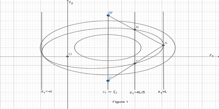
Figure 1. Estimation on lower bound of $l$

Our first main result is the following estimation to upper and lower bounds of width length function. In other words, we will prove the convex body $\Omega$ would be a “round” one rather than a “thin” one, and would be neither “small” nor “large” in the scale.

Theorem 2.1.

For each $p\in(0,2)$ and positive function $f\in C^{\alpha}({\mathbb{S}}^{1})$, there exists a positive constant $C_{p,f}$ depending only on $p$ and $f_{\pm}$, such that

(2.12) $$C_{p,f}^{-1}\leq w_{\Omega_{u}}^{-}\leq w_{\Omega_{u}}^{+}\leq C_{p,f}$$

holds for positive classical solution $u$ of (1.3).

Set $m^{*}$ to be the $z_{1}$ coordinate of ${r}\Big{(}\frac{\pi}{2}\Big{)}$ and define $\theta_{0}-\theta_{1}$ by

$${r}(\theta_{0})=(0,\varphi(0)),\ \ {r}(\theta_{1})=(4L/5,\varphi(4L/5)),$$

where $\varphi(s),s\in[-d,L]$ is the graph function of upper component of boundary $\partial\Omega$. Before proving the theorem, let’s first quote a geometric lemma by Chen-Li [7].

Lemma 2.3.

When $m^{*}>0$, the function ${l(\theta)}$ and $u(\theta)$ are both monotone decreasing functions from $\pi/2$ to $\theta_{0}$. If $m^{*}\leq\frac{3L}{4}$, the function ${l(\theta)}$ and $u(\theta)$ are also both monotone decreasing functions from $\theta_{1}$ to $\pi/2$, as long as

(2.13) $$w_{\Omega_{u}}^{+}/w_{\Omega_{u}}^{-}\geq 100.$$

Proof. The first part in case $m^{*}\geq\frac{L}{2}$ follows from monotone increasing of $\varphi(s)$ on interval $s\in[0,m^{*}]$. To show the second part in case $m^{*}\leq\frac{L}{2}$, one needs only to use the bound

$$|\varphi^{\prime}(s)|\leq 1/10,\ \ \forall s\in[m^{*},4L/5]$$

thanks to the assumption (2.13). $\Box$

Proof of Theorem 2.1. Suppose on the contrary, one may assume that (2.13) holds. When $m^{*}\geq\frac{L}{2}$, by Lemma 2.3 and 2.1, we have

(2.14) $$l^{2}(\pi/2)-l^{2}(\theta_{0})\leq\frac{2f_{+}}{p}\Big{(}u^{p}(\pi/2)-u^{p}(\theta_{0})\Big{)}\leq\frac{2f_{+}}{p}l^{p}.$$

Noting that upon (2.13), there holds also

(2.15) $$l^{2}(\pi/2)-l^{2}(\theta_{0})\geq L^{2}/4-l^{2}\geq L^{2}/5.$$

Another hand, it yields from (2.10) and (2.11) that

(2.16) $$\frac{w_{\Omega_{u}}^{+}}{4}\leq L\leq 2w_{\Omega_{u}}^{+}.$$

Combining (2.14)-(2.16) with

(2.17) $$\frac{w_{\Omega_{u}}^{+}}{2}\leq u_{max}\leq w_{\Omega_{u}}^{+}$$

and Lemma 2.2, one concludes that

(2.18) $$C_{p,f}^{-1}\leq l\leq L\leq C_{p,f}.$$

Thus, a contradiction holds with our assumption by using (2.10), (2.11) and (2.18).

If $m^{*}\leq 3L/4$ and (2.13) holds, we use

(2.19) $$l^{2}(\theta_{1})-l^{2}(\pi/2)\leq\frac{2f_{+}}{p}\Big{(}u^{p}(\theta_{1})-u^{p}(\pi/2)\Big{)}\leq Cl^{p}$$

to replace (2.14) and use

(2.20) $$l^{2}(\theta_{1})-l^{2}(\pi/2)\geq C^{-1}L^{2}$$

to replace (2.15), where

$$\begin{cases}\tan\alpha\equiv\Big{|}\varphi^{\prime}\Big{(}\frac{4L}{5}\Big{)}\Big{|}\leq\frac{l}{L/5},\\ \tan\beta\equiv\frac{\varphi(4L/5)}{4L/5}\leq\frac{l}{4L/5}\end{cases}$$

and

$$u(\theta_{1}) = \sqrt{\Big{(}\frac{4L}{5}\Big{)}^{2}+\varphi^{2}\Big{(}\frac{4L}{5}\Big{)}}\sin(\alpha+\beta)$$

$$\leq \sqrt{(4L/5)^{2}+l^{2}}\sin(\alpha+\beta)\leq CL\cdot\frac{l}{L}=Cl$$

have been used in second inequality of (2.19) (see Figure 2). A similar argument as above gives the positive lower bound of $l$ and thus (2.12) was drawn. $\Box$

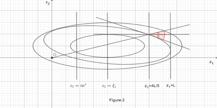
Figure 2. Estimation on lower bound of $l$

3. Arbitrarily smallness of $u_{min}$ for $p\in(0,2)$

Once we obtain the good shape estimation in Theorem 2.1, it would be interesting to ask whether there holds an a-priori lower bound for $u_{min}$. In this section, we shall show that this may not be true in some occasions for $p\in(0,2)$. We have the following theorem.

Theorem 3.1.

For each $p\in(0,2)$, there exists a sequence of $f_{j}$ with uniformly upper and positive lower bound, which is also uniformly bounded in $C^{\alpha}({\mathbb{S}}^{1})$ for some $\alpha\in(0,1)$, such that their corresponding positive classical solutions $u_{j},j\in{\mathbb{N}}$ satisfy

(3.1) $$\min_{{\mathbb{S}}^{1}}u_{j}\to 0^{+},\ \ \mbox{ as }j\to\infty.$$

Proof. For each $\varepsilon>0$ small, we set

$$u(\theta)=(\theta+\varepsilon)^{\frac{2}{2-p}}-\frac{2}{2-p}\varepsilon^{\frac{2}{2-p}-1}\theta,\ \ \theta\in[0,1]$$

to be an increasing positive function on $[0,1]$. Direct computation shows that

(3.2) $$f(\theta) \equiv \frac{u_{\theta\theta}+u}{u^{p-1}}$$

$$= \frac{a_{1}(\theta+\varepsilon)^{\frac{2(p-1)}{2-p}}+g(\theta)}{g^{p-1}(\theta)},$$

where

$$a_{1} \equiv \frac{2}{2-p}\Big{(}\frac{2}{2-p}-1\Big{)},$$

$$g(\theta) \equiv (\theta+\varepsilon)^{\frac{2}{2-p}}-\frac{2}{2-p}\varepsilon^{\frac{2}{2-p}-1}\theta.$$

Using the fact

(3.3) $$\sigma_{p}(\theta+\varepsilon)^{\frac{2}{2-p}}\leq g(\theta)\leq C_{p}(\theta+\varepsilon)^{\frac{2}{2-p}}$$

for $p\in(0,2)$, where $\sigma_{p}$ is a constant closing to 1 and $C_{p}$ is large enough, one has

(3.4) $$\frac{a_{1}+\sigma_{p}(\theta+\varepsilon)^{2}}{C_{p}^{p-1}}\leq f(\theta)\leq\frac{a_{1}+C_{p}(\theta+\varepsilon)^{2}}{\sigma_{p}^{p-1}},\ \ \forall\theta\in[0,1]$$

and

$$u(1) = (1+\varepsilon)^{\frac{2}{2-p}}-\frac{2}{2-p}\varepsilon^{\frac{2}{2-p}-1}$$

(3.5) $$u_{\theta}(1) = \frac{2}{2-p}(1+\varepsilon)^{\frac{2}{2-p}-1}-\frac{2}{2-p}\varepsilon^{\frac{2}{2-p}-1}$$

$$u_{\theta\theta}(1) = a_{1}(1+\varepsilon)^{\frac{2}{2-p}-2}.$$

Next, let’s construct a $C^{2,\alpha}$ function $\varphi$ on $[1,\pi]$ as follows. At first, we set

$$\varphi(1) = (1+\varepsilon)^{\frac{2}{2-p}}-\frac{2}{2-p}\varepsilon^{\frac{2}{2-p}-1}$$

(3.6) $$\varphi_{\theta}(1) = \frac{2}{2-p}(1+\varepsilon)^{\frac{2}{2-p}-1}-\frac{2}{2-p}\varepsilon^{\frac{2}{2-p}-1}$$

$$\varphi_{\theta\theta}(1) = a_{1}(1+\varepsilon)^{\frac{2}{2-p}-2}.$$

and let $\varphi_{\theta\theta}$ decreases rapidly to zero such that $\varphi_{\theta}$ approaches to $\frac{2}{2-p}$ on $(1,2.1)$. As a result, one has

(3.7) $$\begin{cases}\varphi(2.1)\sim\frac{2.2}{2-p}+1,\ \ \varphi_{\theta}(2.1)=\frac{2}{2-p},\\ \varphi_{\theta\theta}(2.1)=0.\end{cases}$$

Next, we let $\varphi_{\theta\theta}$ decreases rapidly to $-\frac{2}{2-p}$ such that $\varphi_{\theta}$ decreases to zero exactly at $\theta=\pi$. Furthermore, we assume that there holds

(3.8) $$-\frac{2}{2-p}\leq\varphi_{\theta\theta}\leq 0,\ \ \theta\in[2.1,\pi],$$

and thus implies that

(3.9) $$\begin{cases}0\leq\varphi_{\theta}\leq\frac{2}{2-p},&\forall\theta\in[2.1,\pi]\\ a_{2}\leq\varphi\leq a_{3},&\forall\theta\in[2.1,\pi]\end{cases}$$

for

$$a_{2}\equiv\frac{2.2}{2-p},\ \ \ \ a_{3}\equiv\frac{2}{2-p}(\pi-1)+2.$$

Therefore, if one sets

$$u(\theta)\equiv\begin{cases}g(\theta),&\theta\in[0,1)\\ \varphi(\theta),&\theta\in(1,\pi]\\ u(-\theta),&\theta\in(-\pi,0),\end{cases}$$

it is easy to verify that $u\in C^{2,\alpha}({\mathbb{S}}^{1})$ for some $\alpha\in(0,1)$. Moreover, when $\theta\in(0,1]$, there holds (3.4). And when $\theta\in(1,2.1]$,

(3.10) $$g^{2-p}(1)\leq f(\theta)\leq\frac{\frac{2.2}{2-p}+1+a_{1}(1+\varepsilon)^{\frac{2}{2-p}-2}}{g^{p-1}(1)}.$$

Finally, if $\theta\in(2.1,\pi]$, one has that

(3.11) $$\frac{\frac{0.2}{2-p}+1}{a_{3}^{p-1}}\leq f(\theta)\leq\frac{a_{3}}{a_{2}^{p-1}}$$

by (3.8) and (3.9). The conclusion of the theorem follows by setting $\varepsilon=\frac{1}{j}$ and then letting $j\to+\infty$. $\Box$

As a corollary of Theorem 3.1, one obtains Theorem 1.2.

4. Invertible Harnack inequality when $p\leq 0$

At the beginning of this section, we will first prove the following invertible Harnack inequality for non-positive $p$.

Theorem 4.1.

Consider (1.3) for $p\leq 0$ and positive function $f\in C^{\alpha}({\mathbb{S}}^{1})$. There exists a positive constant $C_{p,f}$ depending only on $p$ and $f_{\pm}$, such that

(4.1) $$\begin{cases}C_{p,f}^{-1}u_{min}^{p}\leq u^{2}_{max}\leq C_{p,f}u_{min}^{p},&\mbox{ for }p<0,\\ C_{p,f}^{-1}\ln u_{min}^{-1}\leq u^{2}_{max}\leq C_{p,f}\ln u_{\min}^{-1},&\mbox{ for }p=0\end{cases}$$

holds for any positive classical solution $u$.

Our proofs are consisted of two lemmas.

Lemma 4.1.

Under assumptions of Theorem 4.1, there exists a positive constant $C_{p,f}$ such that

(4.2) $$\begin{cases}u_{max}^{2}\leq C_{p,f}u_{min}^{p},&\mbox{ for }p<0,\\ u_{max}^{2}\leq C_{p,f}\ln u_{min}^{-1},&\mbox{ for }p=0.\end{cases}$$

Proof. The lemma is a direct consequence of (2.4) and (2.8) for $p<0$, and a consequence of (2.5) and (2.8) for $p=0$. $\Box$

We have a second lemma under below, which can actually imply a stronger version of Theorem 4.1.

Lemma 4.2.

Under the assumptions of Theorem 4.1, there exists a positive constant $C_{p,f}$ such that

(4.3) $$\begin{cases}u_{min}^{\frac{p}{2}}\leq C_{p,f}\int_{{\mathbb{S}}^{1}}u^{p-1}d\theta,&\mbox{ for }p<0,\\ \sqrt{\ln u_{min}^{-1}}\leq C_{p,f}\int_{{\mathbb{S}}^{1}}u^{-1}d\theta,&\mbox{ for }p=0\end{cases}$$

holds for any positive classical solution $u$ of (1.3).

Proof. Without loss of generality, one may assume that $u_{min}=u(0)$. By (1.3), there holds

$$u_{\theta\theta}(\theta)\leq C_{1}u_{min}^{p-1},\ \ \forall\theta\in[0,2\pi)$$

for some positive constant $C_{1}$. Thus, it follows from Taylor’s expansion formula that

(4.4) $$u(\theta)\leq u_{min}+C_{1}u_{min}^{p-1}\theta^{2},\ \ \forall\theta\in[0,2\pi).$$

As a result, one obtains that

$$\int_{{\mathbb{S}}^{1}}u^{p-1}d\theta \geq \int_{{\mathbb{S}}^{1}}\Big{(}u_{min}+C_{1}u_{min}^{p-1}\theta^{2}\Big{)}^{p-1}d\theta$$

$$\geq C_{2}\int_{{\mathbb{S}}^{1}}\Big{(}u_{min}^{1/2}+C_{3}u_{min}^{(p-1)/2}\theta\Big{)}^{2(p-1)}d\theta$$

$$\geq \frac{C_{2}}{(2p-1)C_{3}}u_{min}^{(1-p)/2}\Big{(}u_{min}^{1/2}+C_{3}u_{min}^{(p-1)/2}\theta\Big{)}^{2p-1}\Big{|}_{0}^{u_{min}^{(1-p)/2}}$$

$$\geq C_{4}u_{min}^{\frac{1-p}{2}}\Big{(}-C_{p,f}^{-1}+u_{\min}^{\frac{2p-1}{2}}\Big{)}\geq C_{5}u_{min}^{\frac{p}{2}}$$

when $p<0$, where (4.4) and Lemma 2.2 have been used. When $p=0$, if $u_{min}$ is not small, then (4.3) is clear true due to (2.8). Hence, one may assume that $u_{min}\ll 1$. Note first that the function

$$F(u)\equiv u^{2}-2f_{+}\ln u$$

is a decreasing function on $(0,\sqrt{f_{+}}]$ and is a increasing function on $[\sqrt{f_{+}},+\infty)$. Moreover,

(4.5) $$\lim_{u\to 0^{+}}F(u)=\lim_{u\to+\infty}F(u)=+\infty.$$

If one denotes $\theta_{2}\in(0,2\pi)$ to be the first critical time of $u$, there must be

(4.6) $$u(\theta_{2})\geq\sqrt{f_{-}}$$

(since $u_{\theta\theta}$ is positive unless $u$ reaches $\sqrt{f_{-}}$ by (1.3)) and

(4.7) $$\theta_{2}\geq C_{p,f}^{-1}\frac{1}{\sqrt{\ln u_{min}^{-1}}},$$

where the second inequality follows from (4.6) and the gradient bound

(4.8) $$0<u_{\theta}\leq C_{p,f}\sqrt{\ln u_{min}^{-1}},\ \ \forall\theta\in[0,\theta_{2})$$

by (2.4). So, one has

(4.9) $$u(\theta)\leq u_{min}+C_{5}\sqrt{\ln u_{min}^{-1}}\theta,\ \ \forall\theta\in[0,\theta_{2})$$

and can conclude that

$$\int_{{\mathbb{S}}^{1}}u^{-1}d\theta \geq \int_{{\mathbb{S}}^{1}}\Big{(}u_{min}+C_{5}\sqrt{\ln u_{min}^{-1}}\theta\Big{)}^{-1}d\theta$$

$$\geq \frac{1}{C_{5}\sqrt{\ln u_{min}^{-1}}}\ln\Big{(}u_{min}+C_{5}\sqrt{\ln u_{min}^{-1}}\theta\Big{)}\Big{|}^{C_{p,f}^{-1}\Big{/}\Big{(}2\sqrt{\ln u_{min}^{-1}}\Big{)}}_{0}$$

$$\geq C_{6}\sqrt{\ln u_{min}^{-1}}.$$

The proof of the lemma was done. $\Box$

Proof of Theorem 4.1. Integrating (1.3) over ${\mathbb{S}}^{1}$, one gets that

(4.10) $$\int_{{\mathbb{S}}^{1}}fu^{p-1}d\theta=\int_{{\mathbb{S}}^{1}}ud\theta.$$

Therefore, it yields from (4.1), (4.3) and (4.10) that

(4.11) $$u_{min}^{\frac{p}{2}}\leq C_{p,f}\int_{{\mathbb{S}}^{1}}u^{p-1}d\theta\leq C_{p,f}\int_{{\mathbb{S}}^{1}}ud\theta\leq C_{p,f}u_{max}\leq C_{p,f}u_{min}^{\frac{p}{2}}$$

for $p<0$ and

(4.12) $$\sqrt{\ln u_{min}^{-1}}\leq C_{p,f}\int_{{\mathbb{S}}^{1}}u^{-1}d\theta\leq C_{p,f}\int_{{\mathbb{S}}^{1}}ud\theta\leq C_{p,f}u_{max}\leq C_{p,f}\sqrt{\ln u_{min}^{-1}}$$

for $p=0$. The proof was done. $\Box$

As in Section 2, we want to prove the following round shape result.

Theorem 4.2.

For each $p\in(-1,0]$ and positive function $f\in C^{\alpha}({\mathbb{S}}^{1})$, there exists a positive constant $C_{p,f}$ depending only on $p$ and $f_{\pm}$, such that

(4.13) $$C_{p,f}^{-1}\leq w_{\Omega_{u}}^{-}\leq w_{\Omega_{u}}^{+}\leq C_{p,f}w_{\Omega_{u}}^{-}$$

holds for positive classical solution $u$ of (1.3).

Adapting the notations and tricks as in Section 2, we will show the following proposition first.

Proposition 4.1.

Under assumptions of Theorem 4.2, there exists a positive constant $C_{p,f}\geq 100$ such that

(4.14) $$w_{\Omega_{u}}^{+}/w_{\Omega_{u}}^{-}\leq C_{p,f}.$$

The next lemma will be used in the proofs of Proposition 4.1 and Theorem 4.2.

Lemma 4.3.

There exists a positive constant $C_{p,f}$ such that

(4.15) $$(w_{\Omega_{u}}^{+})^{1-p}w_{\Omega_{u}}^{-}\geq C_{p,f}^{-1}$$

holds for solution $u$ of (1.3).

Proof. Multiplying (1.3) by $u$ and integrating over ${\mathbb{S}}^{1}$, the area $V(\Omega_{u})$ of $\Omega_{u}$ satisfies that

(4.16) $$V(\Omega_{u})=\int_{{\mathbb{S}}^{1}}u(u_{\theta\theta}+u)d\theta=\int_{{\mathbb{S}}^{1}}fu^{p}\geq 2\pi f_{-}u_{max}^{p}\geq C_{p,f}^{-1}(w_{\Omega_{u}}^{+})^{p}.$$

On the other hand,

(4.17) $$V(\Omega_{u})\leq Cab\leq Cw_{\Omega_{u}}^{+}w_{\Omega_{u}}^{-}$$

holds for $a,b$ defined in (2.10) and universal constant $C>0$. Hence, (4.14) follows from (4.15) and (4.16). $\Box$

Proof of Proposition 4.1. Suppose on the contrary, then

(4.18) $$w_{\Omega_{u}}^{+}/w_{\Omega_{u}}^{-}\geq C_{p,f}\geq 100.$$

When $m^{*}\leq 3L/4$, if $p<0$, there hold

(4.19) $$l^{2}(\theta_{1})-l^{2}(\pi/2)\leq\frac{2f_{+}}{p}\Big{(}u^{p}(\theta_{1})-u^{p}(\pi/2)\Big{)}\leq Cl^{p}$$

and (2.20). So, we have

(4.20) $$L^{2}\leq C_{p,f}l^{p}.$$

Combining (4.20) with (4.15) and (4.18), we conclude that

(4.21) $$C_{p,f}^{-1}\leq l\leq L\leq C_{p,f}$$

and hence (4.14) thanks to $p\in(-1,0)$. If $p=0$, we use

$$l^{2}(\theta_{1})-l^{2}(\pi/2)\leq 2f_{+}\ln\frac{u(\theta_{1})}{u(\pi/2)}\leq 0$$

and (2.20) to conclude contradiction.

If $m^{*}\geq 3L/4$, we define $\theta_{3}\in(\pi/2,\pi)$ by ${r}(\theta_{3})=\Big{(}L/2,\varphi(L/2)\Big{)}$ and define $\theta_{4}\in(\pi,2\pi)$ by ${r}(\theta_{4})=(3L/4,\varphi(3L/4))$. Moreover, we denote

$$\delta_{1}\equiv u(\theta_{3}),\ \ \delta_{2}\equiv u(\theta_{4}).$$

Similarly, one needs also consider the lower portion of boundary $\partial\Omega$ and denote its graph by

$$\widehat{\varphi}(s):\ {r(\theta)}=(s,\widehat{\varphi}(s)),\ \ s\in[\pi,2\pi).$$

we define $\widehat{\theta}_{3}\in(\pi/2,\pi)$ by ${r}(\widehat{\theta}_{3})=\Big{(}L/2,\widehat{\varphi}(L/2)\Big{)}$ and define $\widehat{\theta}_{4}\in(\pi,2\pi)$ by ${r}(\widehat{\theta}_{4})=(3L/4,\widehat{\varphi}(3L/4))$. Parallelly, we can also define

$$\widehat{\delta}_{1}\equiv u(\widehat{\theta}_{3}),\ \ \widehat{\delta}_{2}\equiv u(\widehat{\theta}_{4})$$

and $m_{*}$ to be the $z_{1}$ coordinate of ${r}(3\pi/2)$.

The remaining proofs are divided into several lemmas.

Lemma 4.4.

Under the assumptions of Proposition 4.1 and (4.18), there exists a small constant $\varepsilon\equiv\varepsilon_{p,f}\in(0,1)$ such that if $m^{*}\geq 3L/4$, there holds

(4.22) $$\delta_{1}\equiv u(\theta_{3})\leq\begin{cases}\varepsilon L^{\frac{2}{p}},&p<0,\\ le^{-\varepsilon L^{2}},&p=0.\end{cases}$$

And if $m^{*}\leq 3L/4$, there holds

(4.23) $$\delta_{2}\equiv u(\theta_{4})\leq\begin{cases}\varepsilon L^{\frac{2}{p}},&p<0,\\ le^{-\varepsilon L^{2}},&p=0.\end{cases}$$

Similarly, a same result holds for $m^{*}$ is replaced by $m_{*}$ and $\delta_{1},\delta_{2}$ is replaced by $\widehat{\delta}_{1},\widehat{\delta}_{2}$.

Proof. When $m^{*}\geq 3L/4$, arguing as in Section 2 and using the geometric lemma 2.3, if (4.22) is not true, one has

(4.24) $$l^{2}(\pi/2)-l^{2}(\theta_{3})\leq\frac{2f_{+}}{p}\Big{(}u^{p}(\pi/2)-u^{p}(\theta_{3})\Big{)}\leq\varepsilon L^{2}$$

in case $p<0$ and

(4.25) $$l^{2}(\pi/2)-l^{2}(\theta_{3})\geq(3L/4)^{2}-\Big{(}(L/2)^{2}+l^{2}\Big{)}\geq L^{2}/5$$

by assumption (4.18). Contradiction holds. If $p=0$, we use

$$l^{2}(\pi/2)-l^{2}(\theta_{3})\leq 2f_{+}\ln\frac{u(\pi/2)}{u(\theta_{3})}\leq 0$$

and (4.25) to achieve a similar contradiction.

When $m^{*}\leq 3L/4$, one can use

(4.26) $$l^{2}(\theta_{1})-l^{2}(\theta_{4})\leq\frac{2f_{+}}{p}\Big{(}u^{p}(\theta_{1})-u^{p}(\theta_{4})\Big{)}\leq C_{p,f}u^{p}(\theta_{4})$$

and

(4.27) $$l^{2}(\theta_{1})-l^{2}(\theta_{4})\geq C_{p,f}^{-1}L^{2}$$

to conclude the validity of (4.23) in case $p<0$. For $p=0$,

$$l^{2}(\theta_{1})-l^{2}(\theta_{4})\leq 2f_{+}\ln\frac{u(\theta_{1})}{u^{p}(\theta_{4})}$$

is used to replace (4.26). Together with (4.27), a contradiction yields. The inequalities for lower portion can be proved similarly. $\Box$

Considering an arc interval

$$\omega\equiv\Big{\{}\theta\in(\pi/2,\pi]|\ {r}(\theta)=(s,\varphi(s)),-d\leq s\leq L/2\Big{\}}=(\theta_{3},\pi)$$

and defining

$$\beta(\theta)\equiv\arg({r}(\theta))\in{\mathbb{S}}^{1},\ \ \theta\in{\mathbb{S}}^{1}$$

to be the reverse Gaussian mapping $G^{-1}:{\mathbb{S}}^{1}\to{\mathbb{S}}^{1}$, one has

(4.28) $$\tan(\theta_{3}-\pi/2)\leq\tan\beta(\theta_{3})\leq\frac{l}{L/2}\ll 1$$

and hence

(4.29) $$\Big{\{}\theta|\ 51\pi/100\leq\theta\leq\pi\Big{\}}\subset\omega.$$

Using the expansion relation (2.1), direct computation shows that

(4.30) $$\frac{d\beta}{d\theta}=\frac{u(u+u_{\theta\theta})}{l^{2}},\ \ l^{2}=u^{2}+u_{\theta}^{2}.$$

Therefore, it is inferred from (1.3) and (4.29) that

(4.31) $$\int_{G^{-1}(\omega)}u^{-p}(\beta)l^{2}(\beta)d\beta=\int_{\omega}fd\theta\geq 49\pi f_{-}/100$$

where we denote

$$u(\beta)\equiv u(G(\beta)),\ \ r(\beta)\equiv r(G(\beta))$$

for short. Now, we can deduce a contradiction by estimating L.H.S. of (4.31) using a similar geometric lemma as in [7].

Lemma 4.5.

Under the assumptions of Proposition 4.1, (4.18) and $m^{*}\geq 3L/4$, there exists a positive constant $C_{p,f}$ such that

(4.32) $$\int_{G^{-1}(\omega)}u^{-p}(\beta)r^{2}(\beta)d\beta\leq\begin{cases}C_{p,f}\Big{(}L^{\frac{2}{p}+1-p}+L^{\frac{2(1-p)}{p}}\Big{)},&p<0\\ C_{p,f}\Big{(}L^{2-p}e^{-\varepsilon L^{2}}+(Le^{-\varepsilon L})^{2-p}\Big{)},&p=0.\end{cases}$$

Proof. We will follow the arguments in [7] to prove (4.32) Denoting $l_{P}$ to be the tangential line of $\partial\Omega$ at $P\equiv{r}(\theta_{3})$, and denoting $l_{P}^{\perp}=\overrightarrow{OQ}$ to be the perpendicular ray of $l_{P}$ starting from origin which intersect with $l_{P}$ at $Q$, we set

$$\omega_{1}\equiv\Big{\{}\beta\in G^{-1}(\omega)|\ {r}(G(\beta))\in\triangle OPQ\Big{\}}$$

and

$$\omega_{2}\equiv\Big{\{}\beta\in G^{-1}(\omega)|\ \cos\beta\in[-d,0]\Big{\}}.$$

it is clear that

(4.33) $$G^{-1}(\omega)\subset\omega_{1}\cup\omega_{2}$$

and

(4.34) $$\cup_{t\in[0,1],\beta\in\omega_{1}}\Big{\{}t{r}(\beta)\Big{\}}\subset\triangle OPQ,\ \ \cup_{t\in[0,1],\beta\in\omega_{2}}\Big{\{}t{r}(\beta)\Big{\}}\subset{\mathcal{R}},$$

where ${\mathcal{R}}$ is the rectangular

$${\mathcal{R}}\equiv\Big{\{}(z_{1},z_{2})\in{\mathbb{R}}^{2}|\ z_{1}\in[-d,0],z_{2}\in[-\widehat{h},h]\Big{\}},$$

where

$$h\equiv\varphi(0),\ \ \widehat{h}\equiv-\widehat{\varphi}(0).$$

Figure 3. Estimation on lower bound of $l$

For any $\beta\in\omega_{1}$, let’s define

$$\widetilde{r}\equiv\sup\Big{\{}tr(\beta)|\ t{r}(\beta)\in\triangle OPQ\Big{\}}.$$

For $\beta\in\omega_{2}$, we can also define

$$\widetilde{r}\equiv\sup\Big{\{}tr(\beta)|\ t{r}(\beta)\in{\mathcal{R}}\Big{\}}.$$

Now, we go to estimate

(4.35) $$\int_{\omega_{1}}\widetilde{r}^{2-p}(\beta)d\beta+\int_{\omega_{2}}\widetilde{r}^{2-p}(\beta)d\beta\geq\int_{G^{-1}(\omega)}u^{-p}r^{2}(\beta)d\beta.$$

At first, noting that by (4.22), there holds

(4.36) $$h=\varphi(0)\leq 2|OQ|=2\delta_{1}\leq\begin{cases}2\varepsilon L^{\frac{2}{p}},&\forall p<0\\ 2le^{-\varepsilon L^{2}},&\forall p=0.\end{cases}$$

Similarly, one also has

(4.37) $$\widehat{h}=-\widehat{\varphi}(0)\leq\begin{cases}2\varepsilon L^{\frac{2}{p}},&\forall p<0\\ 2le^{-\varepsilon L^{2}},&\forall p=0.\end{cases}$$

On another hand, by the convexity of $\Omega$, the triangle $\triangle_{0}ABC$ composed of

$$A=(-d,\varphi(-d)),\ \ B=\xi-be_{2},\ \ C=\xi+be^{2}$$

lies entirely inside of $\Omega$. So, one has

$$\frac{d}{L/2}\leq\frac{h+\widehat{h}}{2b}$$

and thus

(4.38) $$d\leq\begin{cases}\varepsilon L^{1+\frac{2}{p}}l^{-1}\leq\varepsilon L^{1+\frac{2}{p}}u_{min}^{-1}\leq\varepsilon L^{1+\frac{2}{p}}u_{max}^{-\frac{2}{p}}\leq\varepsilon L,&p<0\\ CLe^{-\varepsilon L^{2}},&p=0\end{cases}$$

by invertible Harnack inequality (4.1). As a result, we could estimate

$$\int_{\omega_{1}}\widetilde{r}^{2-p}(\beta)d\beta \leq \int^{\frac{\pi}{2}-\arcsin\frac{\delta_{1}}{\sqrt{(L/2)^{2}-l^{2}}}}_{0}\Bigg{(}\frac{\delta_{1}}{\cos\beta}\Bigg{)}^{2-p}d\beta$$

$$\leq C\delta_{1}^{2-p}\int^{\frac{\pi}{2}-\arcsin\frac{\delta_{1}}{\sqrt{(L/2)^{2}+l^{2}}}}_{0}\Big{(}\frac{\pi}{2}-\beta\Big{)}^{p-2}d\beta$$

$$\leq C_{p,f}\delta_{1}L^{1-p}\leq\begin{cases}C_{p,f}L^{\frac{2}{p}+1-p},&p<0\\ C_{p,f}L^{1-p}le^{-\varepsilon L^{2}},&p=0\end{cases}$$

and

$$\int_{\omega_{2}}\widetilde{r}^{2-p}(\beta)d\beta \leq 4\int^{\arcsin\frac{d}{\sqrt{d^{2}+(h+\widehat{h})^{2}}}}_{0}\Big{(}\frac{h}{\cos\beta}\Big{)}^{2-p}d\beta$$

$$\leq C_{p,f}(h^{2-p}+hd^{1-p})\leq\begin{cases}C_{p,f}\Big{(}L^{\frac{2(2-p)}{p}}+L^{\frac{2}{p}+1-p}\Big{)},&p<0\\ C_{p,f}(Le^{-\varepsilon L})^{2-p},&p=0.\end{cases}$$

The proof Lemma 4.5 was completed. $\Box$

Continue the proof of Proposition 4.1. By Lemma 4.5 and noting $p\in(-1,0]$, it follows from (4.31) and (4.32) that

$$C_{p,f}^{-1}\leq\int_{G^{-1}(\omega)}u^{-p}r^{2}(\beta)d\beta\leq C_{p,f}L^{-\sigma_{p}}$$

for some $\sigma_{p}>0$. So, there holds

$$C_{p,f}^{-1}\leq l\leq C_{p,f}L\leq C_{p,f}$$

by (4.15). The conclusion of Proposition 4.1 was drawn. $\Box$

Complete the proof of Theorem 4.2. By Lemma 4.3 and Proposition 4.1, one concludes that

(4.39) $$C_{p,f}^{-1}\leq l\leq C_{p,f}L\leq C_{p,f}l$$

for some positive constant $C_{p,f}$. So, Theorem 4.2 follows from (2.10), (2.11) and (4.39). $\Box$

5. Large body and droplet argument

In the previous section we obtain a round shape result. In order to deduce a positive, two-sided bound on the support function, we need to exclude the possibility of large bodies. Here we show

Theorem 5.1.

Under the assumptions of Theorem 4.2, there exists a positive constant $C_{p,f}$ depending only on $p,\min f$ and $||f||_{C^{\alpha}({\mathbb{S}}^{n})}$, such that

(5.1) $$w_{\Omega_{u}}^{+}\leq C_{p,f}$$

holds for positive classical solution $u$ of (1.3). As a result, there holds

(5.2) $$C_{p,f}^{-1}\leq u_{min}\leq u_{max}\leq C_{p,f}.$$

Inequality (5.2) is a direct consequence of (5.1) by invertible Harnack inequality (4.1). Therefore, the crucial step in proof of Theorem 5.1 consists of establishing (5.1). Under below, We will first blow down the solution to a limiting convex body with droplet shape and then produce a contradiction.

Proof. Supposing that (5.1) is not true for some fixed $p\in(-1,0]$, then given any $k\in{\mathbb{N}}$, there exist a positive function $f_{k}\in C^{\alpha}({\mathbb{S}}^{1}),\alpha\in(0,1)$ satisfying

(5.3) $$C_{0}^{-1}\leq f_{k}\leq C_{0},\ \ ||f_{k}||_{C^{\alpha}({\mathbb{S}}^{1})}\leq C_{0},\ \ \forall k\in{\mathbb{N}}$$

for some positive $C_{0}$ independent of $k$, and a positive classical solution $u_{k}$ to (1.3) such that

(5.4) $$\max_{{\mathbb{S}}^{1}}u_{k}=u_{k}(0)\equiv\lambda_{k}\uparrow+\infty,\ \ \forall k,$$

by rotation if necessary. Applying Theorem 4.2 to $u_{k}$, one has

(5.5) $$C_{p,C_{0}}^{-1}\leq w_{\Omega_{u_{k}}}^{-}\leq w_{\Omega_{u_{k}}}^{+}\leq C_{p,C_{0}}w_{\Omega_{u_{k}}}^{-}$$

for some positive constant $C_{p,C_{0}}$ independent of $k$. Rescaling $u_{k}$ by the function $v_{k}=\lambda_{k}^{-1}u_{k}$, we get a solution to

(5.6) $$\partial_{\theta}^{2}v_{k}+v_{k}=\lambda_{k}^{p-2}f_{k}v_{k}^{p-1}$$

which satisfies that

(5.7) $$v_{k}(0)=\max_{{\mathbb{S}}^{1}}v_{k}=1,\ \ \forall k.$$

Another hand, since $\Omega_{v_{k}}=\lambda_{k}^{-1}\Omega_{u_{k}}$, there holds

(5.8) $$w_{\Omega_{v_{k}}}^{+}=\lambda_{k}^{-1}w_{\Omega_{u_{k}}}^{+},\ \ w_{\Omega_{v_{k}}}^{-}=\lambda_{k}^{-1}w_{\Omega_{u_{k}}}^{-}.$$

Noting that

(5.9) $$w_{\Omega_{u_{k}}}/2\leq\lambda_{k}\leq w_{\Omega_{u_{k}}},$$

it follows from (5.5) and (5.9) that

(5.10) $$C_{1}^{-1}\leq w_{\Omega_{v_{k}}}^{-}\leq w_{\Omega_{v_{k}}}^{+}\leq C_{1}$$

for some positive constant $C_{1}$ independent of $k$. Multiplying (5.6) by $v_{k}$, integrating over ${\mathbb{S}}^{1}$ and then performing integration by parts, one gets that

(5.11) $$\int_{{\mathbb{S}}^{1}}|\partial_{\theta}v_{k}|^{2}=\int_{{\mathbb{S}}^{1}}v_{k}^{2}-\lambda_{k}^{p-2}\int_{{\mathbb{S}}^{1}}f_{k}v_{k}^{p}\leq 2\pi,\ \ \forall k.$$

With the help of Sobolev embedding theorem, we conclude that

(5.12) $$||v_{k}||_{C^{1/2}({\mathbb{S}}^{1})}\leq C_{2},\ \ \forall k$$

for some positive constant $C_{2}$ independent of $k$. By Arzela-Ascoli theorem, there exists a limiting nonnegative function $v_{\infty}\in C^{1/2}({\mathbb{S}}^{1})$, such that for a subsequence of $k$,

(5.13) $$\begin{cases}v_{k}\to v_{\infty},\ \ \mbox{ uniformly on }{\mathbb{S}}^{1},\\ v_{k}\to v_{\infty},\ \ \mbox{ uniformly on }C^{2,\alpha}(P),\ \ P\equiv\Big{\{}\theta\in[0,2\pi)|\ v_{\infty}(\theta)>0\Big{\}},\\ v_{\infty}(0)=\max_{{\mathbb{S}}^{1}}v_{\infty}=1,\ \ \min_{{\mathbb{S}}^{1}}v_{\infty}=0,\ \ v_{\infty}\in H^{1}({\mathbb{S}}^{1}),\\ \partial_{\theta}^{2}v_{\infty}+v_{\infty}=0,\ \ \forall\theta\in P.\end{cases}$$

Noting that the unique solution to

$$\partial^{2}_{\theta}v_{\infty}+v_{\infty}=0,\ \ v_{\infty}(0)=\max_{{\mathbb{S}}^{1}}v_{\infty}=1$$

is given by

(5.14) $$v_{\infty}(\theta)=\cos\theta,\ \ \forall\theta\in(-\pi/2,\pi/2).$$

We claim that

(5.15) $$v_{\infty}(\theta)\equiv-\kappa\cos\theta,\ \ \forall\theta\in[\pi/2,3\pi/2]$$

for some nonnegative constant $\kappa$. In fact, noting that

$$\int_{{\mathbb{S}}^{1}}|\partial_{\theta}u_{k}|^{2}\leq\int_{{\mathbb{S}}^{1}}u_{k}^{2}\Rightarrow\int_{{\mathbb{S}}^{1}}|\partial_{\theta}v_{k}|^{2}\leq\int_{{\mathbb{S}}^{1}}v_{k}^{2},$$

by lower semi-continuity of weak convergence on $H^{1}({\mathbb{S}}^{1})$, one concludes that

(5.16) $$\int_{{\mathbb{S}}^{1}}|\partial_{\theta}v_{\infty}|^{2}\leq\int_{{\mathbb{S}}^{1}}v_{\infty}^{2}.$$

Using (5.14), there holds

(5.17) $$\int^{3\pi/2}_{\pi/2}|\partial_{\theta}v_{\infty}|^{2}\leq\int^{3\pi/2}_{\pi/2}v_{\infty}^{2}.$$

However, since

$$v_{\infty}(\pi/2)=v_{\infty}(3\pi/2)=0,$$

it is inferred from (5.17) and Wirtinger’s inequality that

$$v_{\infty}(\theta)=-\kappa\cos\theta,\ \ \forall\theta\in[\pi/2,3\pi/2].$$

The claim was done. On another hand, sine the convex bodies $\Omega_{v_{k}}$ sub-converges to the convex body $\Omega_{v_{\infty}}$ in weak sense, one has also

(5.18) $$\Omega_{v_{\infty}}\supseteq E_{\infty}\equiv\Bigg{\{}z=(z_{1},z_{2})\in{\mathbb{R}}^{2}\Big{|}\ \frac{(z_{1}-\xi_{1\infty})^{2}}{a_{\infty}^{2}}+\frac{(z_{2}-\xi_{2\infty})^{2}}{b_{\infty}^{2}}=1\Bigg{\}}$$

by (5.10), where $\xi_{\infty}=(\xi_{1\infty},\xi_{2\infty})\in{\mathbb{R}}^{2}$ and $a_{\infty}\geq b_{\infty}$ are positive constants. However, a convex body $\Omega_{v_{\infty}}$ with support function

$$v_{\infty}(\theta)=\begin{cases}\cos\theta,&\forall\theta\in(-\pi/2,\pi/2),\\ -\kappa\cos\theta,&\forall\theta\in[\pi/2,3\pi/2]\end{cases}$$

can only be a degenerate two-sides thin droplet with zero in-radius, which contradiction with (5.18). The proof of Theorem 5.1 was completed. $\Box$

6. Topological degree and Theorem 1.3

In this section, we shall use the a-priori upper/lower bound of positive classical solution of (1.3) to prove the desired solvability result Theorem 1.3. The method of Leray-Schauder’s topological degree has been used by Chou-Wang in [8] for $L_{p}$-Minkowski problem and later developed by Chen-Li in [7] to dual-Minkowski problem. For the convenience of the reader, we will present a proof here. For each $p\in(-1,0]$ and positive function $f\in C^{\alpha}({\mathbb{S}}^{1})$, let’s denote

$$p_{t}\equiv tp,\ \ f_{t}\equiv tf+(1-t),\ \ \forall t\in[0,1]$$

and consider the equation

(6.1) $$u_{\theta\theta}+u=f_{t}u^{p_{t}-1},\ \ \forall\theta\in{\mathbb{S}}^{1}.$$

Setting

(6.2) $$\Gamma\equiv\Big{\{}t\in[0,1]|\ \mbox{there is a positive classical solution to }\eqref{e6.1}\Big{\}},$$

we turn to prove $\Gamma=[0,1]$. As shown in Section 8, the uniqueness of (1.3) with $f\equiv 1$ was not true for the case $p\in(-1,0)$. Thus, to show the desired solvability for $-1<p\leq 0$, we need to utilize a uniqueness result by Chow [5] for $n\geq 1,p=1-n$ and $f\equiv 1$.

Lemma 6.1.

For each $n\geq 1$ and $p=1-n$, the solution of (1.1) with respect to constant function $f\equiv 1$ is unique.

Now, let’s apply the method of topological degree to prove Theorem 1.3 in case of $-1<p\leq 0$. As above, for each $p\in(-1,0]$ and positive function $f\in C^{\alpha}({\mathbb{S}}^{1})$, we consider the equation (6.1).

Proposition 6.1.

For each $-1<p\leq 0$ and $f$ satisfying assumptions of Theorem 5.1, there holds $\Gamma=[0,1]$ for $\Gamma$ defined by (6.2).

Proof. Let’s use topological degree to show $\Gamma=[0,1]$. At first, we define

$${\mathcal{F}}_{t}(u)\equiv u_{\theta\theta}+u-f_{t}u^{p_{t}-1},\ \ \forall t\in[0,1].$$

By Theorem 5.1 and Schauder’s estimates for linear elliptic partial differential equations, there exists a positive constant $C_{*}$ independent of $t$, such that

(6.3) $$C_{*}^{-1}\leq u\leq C_{*},\ \ ||u||_{C^{2,\alpha}({\mathbb{S}}^{1})}\leq C_{*},\ \ \alpha\in(0,1)$$

holds for each zero $u$ of ${\mathcal{F}}_{t}$. So, if one defines

$${\mathcal{O}}\equiv\Big{\{}u\in C^{2,\alpha}({\mathcal{S}}^{1})|\ (2C_{*})^{-1}\leq u\leq 2C_{*},\ \ ||u||_{C^{2,\alpha}({\mathbb{S}}^{1})}\leq C_{*}\Big{\}},$$

it is clear that

$${\mathcal{F}}_{t}^{-1}(0)\cap\partial{\mathcal{O}}=0.$$

Noting that by Chow’s uniqueness result Lemma 6.1, $u_{0}\equiv 1$ is the unique solution to (6.1) with respect to $f_{0}\equiv 1$. Moreover, the linearized equation

(6.4) $$\varphi_{\theta\theta}+\varphi=-\varphi,\ \ \forall\theta\in{\mathbb{S}}^{1}$$

of (6.1) at $t=0,u_{0}\equiv 1$ has only trivial solution $\varphi\equiv 0$ since the unique $2\pi$-periodic function

$$\varphi(\theta)=A\cos\sqrt{2}\theta+B\sin\sqrt{2}\theta$$

is given by $A=B=0$. Thus, the degree

$$deg({\mathcal{F}}_{0},{\mathcal{O}},0)=1\not=0.$$

Combining with the preservation property of topological degree [21, 27], there holds

$$deg({\mathcal{F}}_{t},{\mathcal{O}},0)=deg({\mathcal{F}}_{0},{\mathcal{O}},0)\not=0,\ \ \forall t\in[0,1].$$

So, the solvability of (6.1) for $t\in[0,1]$ holds true. The proof of Proposition 6.1 was done. $\Box$

7. Trigonometric identity for $p\leq-2$

In this section, we turn to prove Theorem 1.4. First, we establish a crucial trigonometric identity for (1.3).

Lemma 7.1.

Given $p\leq-2$ and a nonnegative function $f\in C^{\alpha}({\mathbb{S}}^{1})$ which is piece wise $C^{1}$, then for any positive classical solution $u$ of (1.3), there holds

(7.1) $$\int_{{\mathbb{S}}^{1}}K_{f}(\theta)u^{p}=0,$$

where

(7.2) $$K_{f}(\theta)\equiv(p+2)f\cos 2\theta+f_{\theta}\sin 2\theta.$$

Proof. Multiplying (1.3) by $\cos 2\theta u$, integrating over ${\mathbb{S}}^{1}$ and then forming integration by parts, one gets that

(7.3) $$-\int_{{\mathbb{S}}^{1}}\cos 2\theta u_{\theta}^{2}-\int_{{\mathbb{S}}^{1}}\cos 2\theta u^{2}=\int_{{\mathbb{S}}^{1}}\cos 2\theta fu^{p}.$$

Multiplying again (1.3) by $\sin 2\theta u_{\theta}$, one gets that

(7.4) $$-\int_{{\mathbb{S}}^{1}}\cos 2\theta u_{\theta}^{2}-\int_{{\mathbb{S}}^{1}}\cos 2\theta u^{2}=-\frac{1}{p}\int_{{\mathbb{S}}^{1}}\Big{[}f(\theta)\sin 2\theta\Big{]}_{\theta}u^{p}.$$

Thus, there holds

$$\int_{{\mathbb{S}}^{1}}\Bigg{\{}pf(\theta)\cos 2\theta+\Big{[}f(\theta)\sin 2\theta\Big{]}_{\theta}\Bigg{\}}u^{p}=0,$$

which is equivalent to (7.1) and (7.2). The proof was done. $\Box$

In this section, we always denote

$$t^{\beta}\equiv|t|^{\beta-1}t,\ \ \forall t\not=0$$

and use the relations like

$$t^{\beta-1}\cdot t^{-\beta}=|t|^{-1}\not=t^{-1}$$

to distinguish the usually ones.

Proof of Theorem 1.4. We consider first the case $p=-2$. Letting $f(\theta)=2+\cos 2\theta$ and supposing there is a positive classical solution $u$ of (1.3), one obtains that

$$K_{f}(\theta)=-2\sin^{2}2\theta\leq 0,\ \ K_{f}\not\equiv 0,\ \ \forall\theta\in{\mathbb{S}}^{1}$$

by Lemma 7.1. So, it yields from (7.1) a contradiction

$$0>\int_{{\mathbb{S}}^{1}}K_{f}(\theta)u^{p}=0.$$

The proof for $p=-2$ was completed. To show the non-existence result for $p<-2$, let’s first introduce a positive function by

(7.5) $$\xi(\theta)\equiv\begin{cases}\int^{\pi/4}_{\theta}\sin^{\frac{p}{2}}2\vartheta d\vartheta,&\theta\in(0,\pi/2)\\ \xi(-\theta),&\theta\in(-\pi/2,0)\\ \xi(\theta-\pi),&\theta\in(\pi/2,3\pi/2).\end{cases}$$

It’s easy to see that $\xi$ is a $\pi-$periodic even function on

$${\mathbb{R}}\setminus\{k\pi/2,k\in{\mathbb{Z}}\Big{\}}.$$

Moreover, for $p<-2$, there holds

$$\lim_{\theta\to\frac{k\pi}{2}}\xi(\theta)=+\infty$$

for each $k\in{\mathbb{Z}}$. Now, we need a second lemma.

Lemma 7.2.

For each $p<-2$, the function

$$\phi(\theta)\equiv\begin{cases}|\sin 2\theta|^{-\frac{p+2}{2}}\xi(\theta),&\forall\theta\not=\frac{k\pi}{2},k\in{\mathbb{Z}},\\ -\frac{1}{p+2},&\forall\theta=k\pi,k\in{\mathbb{Z}},\\ \frac{1}{p+2},&\forall\theta=\frac{\pi}{2}+k\pi,k\in{\mathbb{Z}}\end{cases}$$

is a $\pi-$periodic even $Lip({\mathbb{S}}^{1})$ function satisfying

(7.6) $$\phi(\theta)>\frac{1}{p+2},\ \ \forall\theta\in{\mathcal{P}}\equiv[0,2\pi)\setminus\{\pi/2+k\pi\}.$$

Proof. Since $\phi$ is a $\pi-$periodic even function and Lipschitz continuity everywhere $\theta\not=k\pi/2,k\in{\mathbb{Z}}$, let us first show $\phi$ is differentiable at $\theta=0$. The case $\theta=\pi/2$ is similarly. The proof is elementary by L’Hospital’s law. Let’s first prove $\phi$ is continuous at $\theta=0$. In fact,

$$\lim_{\theta\to 0}\phi(\theta) = \lim_{\theta\to 0}\frac{\int^{\pi/4}_{\theta}\sin^{\frac{p}{2}}2\vartheta d\vartheta}{(2\theta)^{\frac{p+2}{2}}}$$

$$= \lim_{\theta\to 0}-\frac{\sin^{\frac{p}{2}}2\theta}{(p+2)(2\theta)^{\frac{p}{2}}}=-\frac{1}{p+2}.$$

So $\phi$ is continuous. Next, we show that $\phi$ is differentiable at $\theta=0$. In fact, since

$$\lim_{\theta\to 0}\frac{\phi(\theta)+\frac{1}{p+2}}{\theta} = \lim_{\theta\to 0}\frac{\int^{\pi/4}_{\theta}\sin^{\frac{p}{2}}2\vartheta d\vartheta+\frac{1}{p+2}\sin^{\frac{p+2}{2}}2\theta}{\theta\sin^{\frac{p+2}{2}}2\theta}$$

$$= \lim_{\theta\to 0}\frac{-\sin^{\frac{p}{2}}2\theta+\sin^{\frac{p}{2}}2\theta\cos 2\theta}{(p+4)2^{\frac{p}{2}}\theta^{\frac{p+2}{2}}}$$

$$= \lim_{\theta\to 0}\frac{-1+\cos 2\theta}{(p+4)\theta}=0,$$

$\phi$ is a $Lip({\mathbb{S}}^{1})$ function which is greater than $\frac{1}{p+2}$ everywhere $\theta\in{\mathcal{P}}$. $\Box$

Now, we define

$$f(\theta)\equiv-\frac{1}{p+2}+\phi(\theta),\ \ \forall\theta\in{\mathbb{S}}^{1}$$

to be a positive Lipschitz function outside two polar of ${\mathbb{S}}^{1}$. Direct calculation shows that

$$K_{f}(\theta) = (p+2)\Bigg{(}-\frac{1}{p+2}+\sin^{-\frac{p+2}{2}}2\theta\int^{\pi/4}_{\theta}\sin^{\frac{p}{2}}2\vartheta d\vartheta\Bigg{)}\cos 2\theta$$

$$-(p+2)\sin^{-\frac{p+4}{2}}2\theta\cos 2\theta\int^{\pi/4}_{\theta}\sin^{\frac{p}{2}}2\vartheta d\vartheta\cdot\sin 2\theta-1$$

$$= -1-\cos 2\theta<0,\ \ \forall\theta\in(0,\pi/2).$$

Since $K_{f}$ is $\pi$-periodical even function, (7) is in conflict with (7.1). The proof of Theorem 1.4 was completed. $\Box$

8. Uniqueness for constant $f$

In this section, let’s complete the proof of Theorem 1.5. We assume that $u(0)=u_{min}$ by rotation if necessary and denote it to be $m$ for short. Multiplying (1.3) by $u_{\theta}$, integrating over ${\mathbb{S}}^{1}$ and then performing integration by parts, it yields that

(8.1) $$u_{\theta}^{2}+u^{2}-\frac{2}{p}u^{p}\equiv m^{2}-\frac{2}{p}m^{p},\ \ \forall\theta\in{\mathbb{S}}^{1}$$

for $p\not=0$ and

(8.2) $$u_{\theta}^{2}+u^{2}-2\ln u\equiv m^{2}-2\ln m,\ \ \forall\theta\in{\mathbb{S}}^{1}$$

for $p=0$. Setting

$$F(u)\equiv\begin{cases}u^{2}-\frac{2}{p}u^{p},&p\not=0,\\ u^{2}-2\ln u,&p=0,\end{cases}$$

it is clear that $F$ is monotone decreasing on $(0,1]$ and monotone increasing on $[1,+\infty)$. Moreover,

(8.3) $$\lim_{u\to 0+}F(u)=\begin{cases}0,&p\in(0,2)\\ +\infty,&p\leq 0,\end{cases}$$

$$\lim_{u\to+\infty}F(u)=+\infty,\ \ \forall p<2,p\not=0.$$

On the other hand, it follows from the maximum principle that for non-constant solution $u$, there holds

(8.4) $$m=\min_{{\mathbb{S}}^{1}}u<1,\ \ M\equiv\max_{{\mathbb{S}}^{1}}u>1.$$

By (8.1)-(8.2) and picture of $F$, it is clear that

(8.5) $$F(m)=F(M),\ \ u\uparrow\mbox{ from }m\mbox{ to }M,\mbox{ and }u\downarrow\mbox{ from }M\mbox{ to }m.$$

Furthermore, using the uniqueness of first order ordinary differential equation (8.1)-(8.2) and a reflection $v(\theta)=u(-\theta)$, one can deduce that $u$ must be symmetric around $\theta=\pi$ and thus

(8.6) $$u_{\theta}(\pi)=0.$$

Therefore, it is inferred from (8.1)-(8.2) that any possible non-constant solution of (1.3) must satisfy the compatible condition

(8.7) $$\begin{cases}\int^{M}_{m}\frac{du}{\sqrt{F(m)-F(u)}}=\pi/\kappa,\\ F(m)=F(M)\end{cases}$$

for some positive integer $\kappa$. In fact, one has the following proposition.

Proposition 8.1.

Supposing that $p<2$ and $f\equiv 1$, (1.3) has a positive classical solution $u$ satisfying $u_{min}=m\in(0,1)$ if and only if there exists a pair $(m,M),M>1$ satisfying (8.7) with some $\kappa\in{\mathbb{N}}$.

For any $m\in(0,1)$ and letting $M=M(m)>1$ being the unique positive constant determined by the second relation in (8.7), we define

$$H(m)\equiv\int^{M(m)}_{m}\frac{du}{\sqrt{F(m)-F(u)}}.$$

As shown below, $H$ is a $C^{1}$-function on $(0,1)$. Furthermore, the following lemma would be useful in proving of Theorem 1.5.

Lemma 8.1.

Letting $p<2$, there holds

$$\lim_{m\to 0^{+}}H(m) = \begin{cases}\frac{\pi}{2-p},&\forall p\in(0,2)\\ \pi/2,&\forall p\in(-\infty,0],\end{cases}$$

$$\lim_{m\to 1^{-}}H(m) = \frac{\pi}{\sqrt{2-p}},\ \ \forall p<2.$$

Proof. We consider the case $0<p<2$ first. Since $M(m)\to\Big{(}\frac{2}{p}\Big{)}^{1/(2-p)}$ as $m$ tends to zero, one has

$$\lim_{m\to 0^{+}}H(m) = \int^{\big{(}\frac{2}{p}\big{)}^{1/(2-p)}}_{0}\frac{du}{\sqrt{\frac{2}{p}u^{p}-u^{2}}}$$

$$= \frac{2}{2-p}\arcsin\frac{u^{\frac{2-p}{2}}}{\sqrt{2/p}}\Bigg{|}^{\big{(}\frac{2}{p}\big{)}^{1/(2-p)}}_{0}=\frac{\pi}{2-p}.$$

To calculate the limit at $m=1$, we first use the Cauchy’s mean value theorem to deduce that

$$\frac{(m^{2}-2m)-(u^{2}-2u)}{(m^{2}-\frac{2}{p}m^{p})-(u^{2}-\frac{2}{p}u^{p})}=\frac{2\xi-2}{2\xi-2\xi^{p-1}}\sim\frac{1}{2-p},\ \ \xi\in(m,u).$$

Therefore,

$$\lim_{m\to 1^{-}}H(m) = \lim_{m\to 1^{-}}\frac{1}{\sqrt{2-p}}\int^{M(m)}_{m}\frac{du}{\sqrt{(m-1)^{2}-(u-1)^{2}}}$$

$$= \lim_{m\to 1^{-}}-\frac{1}{\sqrt{2-p}}\arcsin\frac{u-1}{m-1}\Big{|}^{M(m)}_{m}$$

$$= \lim_{m\to 1^{-}}\frac{1}{\sqrt{2-p}}\Bigg{(}\arcsin\frac{M(m)-1}{1-m}+\frac{\pi}{2}\Bigg{)}=\frac{\pi}{\sqrt{2-p}}$$

for any $p<2$, where

$$\lim_{M\to 1^{+}}\frac{(M-1)^{2}}{M^{2}-\frac{2}{p}M^{p}-F(1)}=\lim_{m\to 1^{-}}\frac{(m-1)^{2}}{m^{2}-\frac{2}{p}m^{p}-F(1)}=\frac{1}{2-p},\ \ p\not=0$$

$$\lim_{M\to 1^{+}}\frac{(M-1)^{2}}{M^{2}-2\ln M-1}=\lim_{m\to 1^{-}}\frac{(m-1)^{2}}{m^{2}-2\ln m-1}=\frac{1}{2},\ \ p=0$$

and second relation of (8.7) have been used. Now, let’s calculate the limit at $m=0$ for $p\leq 0$. In fact, for each fixed $\varepsilon>0$, if $m$ is chosen small, $\frac{1}{\sqrt{F(m)-F(u)}}$ is also small on the fixed interval $[0,\varepsilon^{-1}]$. On another hand, one also has

$$F(m) = \begin{cases}(1+o_{\varepsilon}(1))\Big{(}-\frac{2}{p}m^{p}-u^{2}\Big{)},&p<0\\ (1+o_{\varepsilon}(1))\Big{(}-2\ln m-u^{2}\Big{)},&p=0\end{cases}$$

$$= (1+o_{\varepsilon}(1))(M^{2}-u^{2}),\ \ \forall u\geq\varepsilon^{-1},$$

where $o_{\varepsilon}(1)$ is a small quantity as long as $\varepsilon$ is small. So, we obtain that

$$H(m) = o_{m}(1)+(1+o_{\varepsilon}(1))\int^{M(m)}_{\varepsilon^{-1}}\frac{du}{\sqrt{M^{2}-u^{2}}}$$

$$+\begin{cases}(1+o_{\varepsilon}(1))\sqrt{\frac{|p|}{2}}\int^{\varepsilon}_{m}\frac{du}{\sqrt{m^{p}-u^{p}}},&p<0\\ (1+o_{\varepsilon}(1))\sqrt{\frac{1}{2}}\int^{\varepsilon}_{m}\frac{du}{\sqrt{\ln m^{-1}-\ln u^{-1}}},&p=0\end{cases}$$

$$= o_{m}(1)+(1+o_{\varepsilon}(1))\Bigg{(}\arcsin\frac{u}{M(m)}\Big{|}^{M(m)}_{\varepsilon^{-1}}+R(m,\varepsilon)\Bigg{)}$$

$$= o_{m,\varepsilon}(1)+(1+o_{\varepsilon}(1))\Big{(}\pi/2-\arcsin\frac{\varepsilon^{-1}}{M(m)}\Big{)}$$

for small quantity $o_{m,\varepsilon}(1)$ with respect to $m,\varepsilon$, where

$$R(m,\varepsilon) \equiv \sqrt{\frac{|p|}{2}}\int^{\varepsilon}_{m}\frac{du}{\sqrt{m^{p}-u^{p}}}\leq\sqrt{\frac{|p|}{2}}\varepsilon^{\frac{2-p}{2}}\int^{\varepsilon}_{m}\frac{u^{\frac{p-2}{2}}du}{\sqrt{m^{p}-u^{p}}}$$

$$= -\sqrt{\frac{2}{|p|}}\varepsilon^{\frac{2-p}{2}}\arcsin{\Big{(}\frac{u}{m}\Big{)}^{\frac{p}{2}}}\Big{|}^{\varepsilon}_{m}=\sqrt{\frac{2}{|p|}}\varepsilon^{\frac{2-p}{2}}\Bigg{(}\frac{\pi}{2}-\arcsin\Big{(}\frac{\varepsilon}{m}\Big{)}^{\frac{p}{2}}\Bigg{)}=o_{\varepsilon}(1)$$

for $p<0$ and

$$R(m,\varepsilon) \equiv \sqrt{\frac{1}{2}}\int^{\varepsilon}_{m}\frac{du}{\sqrt{\ln u-\ln m}}\leq\sqrt{\frac{1}{2}}\varepsilon\sqrt{\ln\varepsilon^{-1}}\int^{\varepsilon}_{m}\frac{\frac{1}{u\sqrt{-\ln u}}du}{\sqrt{\ln u-\ln m}}$$

$$= -\varepsilon\sqrt{\ln\varepsilon^{-1}}\arcsin\sqrt{\frac{\ln u}{\ln m}}\Big{|}^{\varepsilon}_{m}=\varepsilon\sqrt{\ln{\varepsilon^{-1}}}\Bigg{(}\frac{\pi}{2}-\arcsin\sqrt{\frac{\ln\varepsilon}{\ln m}}\Bigg{)}=o_{\varepsilon}(1)$$

for $p=0$ have been used. Thus, the limit

$$\lim_{m\to 0^{+}}H(m)=\pi/2$$

was shown for $p\leq 0$ and the conclusion was drawn. $\Box$

To proceed further, let’s differentiate the second relation of (8.7) on $m$ and derive that

(8.8) $$\frac{dM}{dm}=\frac{m-m^{p-1}}{M-M^{p-1}}.$$

To differentiate the first relation on (8.7), let’s first perform integration by parts to yields

$$H(m) = \int^{M}_{1+\sigma}\frac{du}{\sqrt{F(M)-F(u)}}+\int^{1-\sigma}_{m}\frac{du}{\sqrt{F(m)-F(u)}}+\int^{1+\sigma}_{1-\sigma}\frac{du}{\sqrt{F(m)-F(u)}}$$

$$= \int^{M}_{1+\sigma}\sqrt{F(M)-F(u)}d\frac{1}{u-u^{p-1}}+\int^{1-\sigma}_{m}\sqrt{F(m)-F(u)}d\frac{1}{u-u^{p-1}}$$

$$+\frac{\sqrt{F(m)-F(1+\sigma)}}{(1+\sigma)-(1+\sigma)^{p-1}}-\frac{\sqrt{F(m)-F(1-\sigma)}}{(1-\sigma)-(1-\sigma)^{p-1}}+\int^{1+\sigma}_{1-\sigma}\frac{du}{\sqrt{F(m)-F(u)}}.$$

Differentiating on $m$, there holds

$$\frac{dH}{dm} = \int^{M}_{1+\sigma}\frac{m-m^{p-1}}{\sqrt{F(m)-F(u)}}d\frac{1}{u-u^{p-1}}+\int^{1-\sigma}_{m}\frac{m-m^{p-1}}{\sqrt{F(m)-F(u)}}d\frac{1}{u-u^{p-1}}$$

$$+\frac{m-m^{p-1}}{(1+\sigma)-(1+\sigma)^{p-1}}\frac{1}{\sqrt{F(m)-F(1+\sigma)}}-\int^{1+\sigma}_{1-\sigma}\frac{(m-m^{p-1})du}{(F(m)-F(u))^{3/2}}$$

$$-\frac{m-m^{p-1}}{(1-\sigma)-(1-\sigma)^{p-1}}\frac{1}{\sqrt{F(m)-F(1-\sigma)}}$$

$$\equiv(m-m^{p-1})\Big{(}J_{1}+J_{2}+J_{3}+J_{4}+J_{4}\Big{)}$$

for a fixed small constant $\sigma>0$. Setting $G(u)\equiv F(u)-F(1)$, it yields that

$$\int^{1+\sigma}_{1}\frac{du}{(F(m)-F(u))^{\frac{3}{2}}}=\int^{1+\sigma}_{1}\frac{du}{(G(m)-G(u))^{\frac{3}{2}}}=\int^{1+\sigma}_{1}\frac{\frac{1}{G^{\frac{3}{2}}(u)}}{\Big{(}\frac{G(m)}{G(u)}-1\Big{)}^{\frac{3}{2}}}du$$

$$\ \ \ \ \ \ \ \ \ \ \ \ \ \ =-\frac{1}{G(m)}\int^{1+\sigma}_{1}\frac{\frac{\sqrt{G(u)}}{G^{\prime}(u)}d\frac{G(m)}{G(u)}}{\Big{(}\frac{G(m)}{G(u)}-1\Big{)}^{\frac{3}{2}}}=\frac{2}{G(m)}\int^{1+\sigma}_{1}\frac{\sqrt{G(u)}}{G^{\prime}(u)}d\frac{1}{\sqrt{\frac{G(m)}{G(u)}-1}}$$

$$= \frac{2G(1+\sigma)}{G(m)G^{\prime}(1+\sigma)}\frac{1}{\sqrt{G(m)-G(1+\sigma)}}-\frac{2}{G(m)}\int^{1+\sigma}_{1}\frac{\frac{1}{2}-\frac{G(u)}{(G^{\prime}(u))^{2}}G^{\prime\prime}(u)}{\sqrt{G(m)-G(u)}}du,$$

where

$$\lim_{u\to 1^{+}}\frac{\sqrt{G(u)}}{G^{\prime}(u)}=\frac{1}{2\sqrt{2-p}}$$

has been used. Similarly, there holds

$$\int^{1}_{1-\sigma}\frac{du}{(F(m)-F(u))^{\frac{3}{2}}} = -\frac{2G(1-\sigma)}{G(m)G^{\prime}(1-\sigma)}\frac{1}{\sqrt{G(m)-G(1-\sigma)}}$$

$$-\frac{2}{G(m)}\int^{1}_{1-\sigma}\frac{\frac{1}{2}-\frac{G(u)}{(G^{\prime}(u))^{2}}G^{\prime\prime}(u)}{\sqrt{G(m)-G(u)}}du.$$

So,

(8.10) $$J_{3}+J_{4}+J_{5} = \frac{2\sqrt{G(m)-G(1+\sigma)}}{G^{\prime}(1+\sigma)G(m)}-\frac{2\sqrt{G(m)-G(1-\sigma)}}{G^{\prime}(1-\sigma)G(m)}$$

$$+\frac{2}{G(m)}\int^{1+\sigma}_{1-\sigma}\frac{\frac{1}{2}-\frac{G(u)}{(G^{\prime}(u))^{2}}G^{\prime\prime}(u)}{\sqrt{G(m)-G(u)}}du.$$

On another hand, there hold

$$J_{1} = -2\int^{M}_{1+\sigma}\frac{G^{\prime\prime}(u)/(G^{\prime}(u))^{2}}{\sqrt{G(m)-G(u)}}du=\frac{2}{G(m)}\int^{M}_{1+\sigma}\frac{\frac{G^{3/2}(u)G^{\prime\prime}(u)}{(G^{\prime}(u))^{3}}d\frac{G(m)}{G(u)}}{\sqrt{\frac{G(m)}{G(u)}-1}}$$

$$= \frac{4}{G(m)}\int^{M}_{1+\sigma}\frac{G^{3/2}(u)G^{\prime\prime}(u)}{(G^{\prime}(u))^{3}}d\sqrt{\frac{G(m)}{G(u)}-1}$$

$$= -\frac{4}{G(m)}\frac{G(1+\sigma)G^{\prime\prime}(1+\sigma)}{(G^{\prime}(1+\sigma))^{3}}\sqrt{G(m)-G(1+\sigma)}$$

$$-\frac{4}{G(m)}\int^{M}_{1+\sigma}\frac{GG^{\prime}G^{\prime\prime\prime}+\frac{3}{2}(G^{\prime})^{2}G^{\prime\prime}-3G(G^{\prime\prime})^{2}}{(G^{\prime})^{4}}\sqrt{G(m)-G(u)}du$$

and

$$J_{2} = \frac{4}{G(m)}\frac{G(1-\sigma)G^{\prime\prime}(1-\sigma)}{(G^{\prime}(1-\sigma))^{3}}\sqrt{G(m)-G(1-\sigma)}$$

$$-\frac{4}{G(m)}\int^{1-\sigma}_{m}\frac{GG^{\prime}G^{\prime\prime\prime}+\frac{3}{2}(G^{\prime})^{2}G^{\prime\prime}-3G(G^{\prime\prime})^{2}}{(G^{\prime})^{4}}\sqrt{G(m)-G(u)}du$$

Summation as above, one concludes that

$$\frac{dH/dm}{m-m^{p-1}} = J_{1}+J_{2}+J_{3}+J_{4}+J_{5}$$

$$= \frac{-4G(1+\sigma)G^{\prime\prime}(1+\sigma)+2(G^{\prime}(1+\sigma))^{2}}{G(m)(G^{\prime}(1+\sigma))^{3}}\sqrt{G(m)-G(1+\sigma)}$$

$$+\frac{4G(1-\sigma)G^{\prime\prime}(1-\sigma)-2(G^{\prime}(1-\sigma))^{2}}{G(m)(G^{\prime}(1-\sigma))^{3}}\sqrt{G(m)-G(1-\sigma)}$$

$$-\frac{4}{G(m)}\int_{[m,M]\setminus(1-\sigma,1+\sigma)}\frac{GG^{\prime}G^{\prime\prime\prime}+\frac{3}{2}(G^{\prime})^{2}G^{\prime\prime}-3G(G^{\prime\prime})^{2}}{(G^{\prime})^{4}}\sqrt{G(m)-G(u)}du$$

$$+\frac{2}{G(m)}\int^{1+\sigma}_{1-\sigma}\frac{\frac{1}{2}-\frac{G(u)}{(G^{\prime}(u))^{2}}G^{\prime\prime}(u)}{\sqrt{G(m)-G(u)}}du.$$

Using again integration by parts,

$$\frac{2}{G(m)}\int^{1+\sigma}_{1-\sigma}\frac{\frac{1}{2}-\frac{G(u)}{(G^{\prime}(u))^{2}}G^{\prime\prime}(u)}{\sqrt{G(m)-G(u)}}du=\frac{-2(G^{\prime})^{2}+4GG^{\prime\prime}}{G(m)(G^{\prime})^{3}}\sqrt{G(m)-G(u)}\Big{|}^{1+\sigma}_{1-\sigma}$$

$$\ \ \ \ \ \ \ \ \ \ \ \ \ \ \ \ \ \ \ +\frac{2}{G(m)}\int^{1+\sigma}_{1-\sigma}\Bigg{[}\frac{(G^{\prime})^{2}-2GG^{\prime\prime}}{(G^{\prime})^{3}}\Bigg{]}_{u}\sqrt{G(m)-G(u)}du.$$

Hence, we arrive at the following relation formula.

Proposition 8.2.

For each $m\in(0,1)$ and $M(m)$ determined by second relation of (8.7), the $C^{1}(0,1)-$function defined by

$$H(m)\equiv\int^{M(m)}_{m}\frac{du}{\sqrt{F(m)-F(u)}},\ \ \forall 0<m<1$$

satisfies an intrinsic relation

(8.11) $$-\frac{G(m)dH/dm}{4(m-m^{p-1})}=\int^{M}_{m}\frac{K(u)}{(G^{\prime}(u))^{4}}\sqrt{G(m)-G(u)}du$$

with the kernel

$$K(u)\equiv GG^{\prime}G^{\prime\prime\prime}+\frac{3}{2}(G^{\prime})^{2}G^{\prime\prime}-3G(G^{\prime\prime})^{2}.$$

Remark 8.1 It is remarkable to note that $u=1$ is a removable singularity of the function $K(u)/(G^{\prime}(u))^{4}$ as shown below. Another hand, after integration by parts, one can obtain another intrinsic identity

(8.12) $$\frac{G(m)dH/dm}{m-m^{p-1}}=\int^{M}_{m}\frac{(G^{\prime})^{2}-2GG^{\prime\prime}}{(G^{\prime})^{2}}\frac{1}{\sqrt{G(m)-G(u)}}du$$

using the relation

(8.13) $$-2\frac{K(u)}{(G^{\prime}(u))^{4}}=\Bigg{[}\frac{(G^{\prime})^{2}-2GG^{\prime\prime}}{(G^{\prime})^{3}}\Bigg{]}^{\prime}_{u}.$$

To proceed further, we note that by direct calculation, the kernel

$$K(u)\equiv GG^{\prime}G^{\prime\prime\prime}+\frac{3}{2}(G^{\prime})^{2}G^{\prime\prime}-3G(G^{\prime\prime})^{2}$$

satisfies that

$$K^{\prime}(u) = \frac{4(p-1)(p-2)}{pu^{1-p}}L(u),$$

(8.14) $$\Big{(}u^{3}L^{\prime}(u)\Big{)}^{\prime} = 2(p-2)u^{p-3}T(u),$$

$$T^{\prime}(u)/p = 2u\Big{\{}(p-1)(3p-4)u^{p-2}-(2p^{2}-7p+8)\Big{\}}$$

where

$$L(u) \equiv (3p-4)u^{2p-4}+2(2p-1)(p-2)u^{p-4}$$

$$+(p-2)(p-8)u^{-2}-2(2p^{2}-7p+8)u^{p-2}-p(p-3)$$

$$T(u) \equiv 2(p-1)(3p-4)u^{p}+(p-2)(p-4)(2p-1)$$

$$-p(2p^{2}-7p+8)u^{2}$$

satisfies that

(8.15) $$K(1)=L(1)=L^{\prime}(1)=T(1)=0.$$

As a result, we have the following monotone result of $H$.

Lemma 8.2.

For $p\in(1,2)$, the function $H(m)$ is a monotone decreasing function on $m\in(0,1)$. While, for $p\in[1/2,1)$, the function $H(m)$ is a monotone increasing function on $m\in(0,1)$.

Proof. When $1\leq p\leq 4/3$, there holds

(8.16) $$T^{\prime}(u)/p = 2u\Big{\{}(p-1)(3p-4)u^{p-2}-(2p^{2}-7p+8)\Big{\}}$$

$$\leq u(p-2)(3p^{2}-5p+8)<0,\ \ \forall u\in\Bigg{(}0,\Bigg{(}\frac{2}{p}\Bigg{)}^{\frac{1}{2-p}}\Bigg{)}$$

So, we conclude that $K/(G^{\prime})^{4}$ is a continuous negative function on

$$\Bigg{(}0,\Bigg{(}\frac{2}{p}\Bigg{)}^{\frac{1}{2-p}}\Bigg{)}\setminus\{1\}$$

for $1<p\leq 4/3$. Thus, the lemma follows by (8.11).

For $p\in(0,2)\setminus[1,4/3]$, noting that (8.16) and (8.15), one has that

(8.17) $$T^{\prime}(u)/p\leq 2u(p^{2}-4)\leq 0,\ \ \forall u>1\Rightarrow T(u)<0,\ \ \forall u>1.$$

Another hand, since $T^{\prime}$ vanishes at a unique point $u_{0}\in(0,1)$, and

$$T^{\prime}(u)=\begin{cases}>0,&\forall u\in(0,u_{0})\\ <0,&\forall u>u_{0},\end{cases}$$

there holds

(8.18) $$T(u) \geq \min\Big{\{}T(0),T(1)\Big{\}}$$

$$= \min\Big{\{}(p-2)(p-4)(2p-1),0\Big{\}}=0,\ \ \forall u\in(0,1)$$

as long as $p\in[1/2,2)$. Consequently, it follows from $K(1)=K^{\prime}(1)=L(1)=L^{\prime}(1)=0$ and (8.17)-(8.18) that

(8.19) $$K(u)<0,\ \ \forall u\in\Big{(}0,(2/p)^{\frac{1}{2-p}}\Big{)}\setminus\{1\}$$

in case of $p\in(1,2)$ and

(8.20) $$K(u)>0,\ \ \forall u\in\Big{(}0,(2/p)^{\frac{1}{2-p}}\Big{)}\setminus\{1\}$$

in case of $p\in[1/2,1)$. Hence, we obtain that the monotonicity of $H$ by (8.11) and (8.19)-(8.20). $\Box$

We also have the following monotonicity of $H$ at the end point $m=1$.

Lemma 8.3.

For $p\in(-\infty,2)\setminus\{1,-2\}$, one has

(8.21) $$\frac{dH}{dm}=\begin{cases}<0,&p\in(1,2)\\ >0,&p\in(-2,1)\\ <0,&p\in(-\infty,-2)\end{cases}$$

for $0<1-m\ll 1$.

Proof. To calculate the sign of derivative of $H$ near $m=1$, we use the first relation (8.11). In fact, for $m$ closing to $1$, one has

$$-\frac{G(m)dH}{4(m-m^{p-1})dm} = \int^{M}_{m}\frac{K(u)}{(G^{\prime}(u))^{4}}\sqrt{G(m)-G(u)}du$$

$$= \begin{cases}<0,&p\in(1,2)\\ >0,&p\in(-2,1)\\ <0,&p\in(-\infty,-2)\end{cases}$$

for all $0<1-m\ll 1$, where

$$\lim_{u\to 1}T^{\prime}(u)/p=2u(p^{2}-4)\begin{cases}<0,&p\in(-2,2)\\ >0,&p\in(-\infty,-2)\end{cases}$$

have been used. The proof of the lemma was done. $\Box$

Remark 8.2 For any $\gamma\in(0,G(m))$, we denote $u\in(m,1),v\in(1,M(m))$ by

$$G(u)=G(v)=\gamma,$$

where $M(m)$ is determined by second relation in (8.7). It is inferred from (8.12) that

(8.22) $$\frac{G(m)dH/dm}{m-m^{p-1}}=-\int^{G(m)}_{0}\mathcal{K}(u,v)\frac{d\gamma}{\sqrt{G(m)-\gamma}},$$

where

$$\mathcal{K}(u,v)\equiv\frac{(G^{\prime}(u))^{2}-2G(u)G^{\prime\prime}(u)}{(G^{\prime}(u))^{3}}-\frac{(G^{\prime}(v))^{2}-2G(v)G^{\prime\prime}(v)}{(G^{\prime}(v))^{3}}.$$

Therefore, one gets the following proposition.

Proposition 8.3.

Suppose that for some $p<2,p\not=1$,

(8.23) $${\mathcal{K}}(u,v)\ \mbox{ doesn't change sign on curve }{\mathcal{L}}$$

holds for curve defined by

(8.24) $${\mathcal{L}}\equiv\Big{\{}(u,v)\in{\mathbb{R}}^{2}|\ G(u)=G(v),\ \ u\in(m,1),v\in(1,M(m))\Big{\}}.$$

We have $H$ is a monotone function on $m\in(0,1)$.

It is remarkable that Proposition 8.3 reduces an uniqueness problem to a purely algebraic condition (8.23) on $G(\cdot)$. Moreover, it is not hard to verify that for $p\in[1/2,2)$, the assumption of Proposition 8.3 holds true since

$$\frac{(G^{\prime})^{2}-2GG^{\prime\prime}}{(G^{\prime})^{3}}$$

is a monotone function on $(m,M(m))$ by (8.13) and the sign of $K$ in proof of Lemma 8.2.

Now, let’s complete the proof of Theorem 1.5 as below.

Proof of Theorem 1.5. We note first that

$$0<2-p<\sqrt{2-p}<1$$

for $p\in(1,2)$, and

$$1<\sqrt{2-p}<2-p<2$$

for $p\in[1/2,1)$. By combining with the monotonicity of $H$ (Lemma 8.2), one concludes the non-existence of non-trivial positive classical solution of (1.3) for $p\in[1/2,1)\cup(1,2)$ after applying Proposition 8.1.

When $p=1$, solving the linear ordinary differential equation (1.3) of second order, one can deduce that all positive classical solutions are given by

(8.25) $$h(\theta)=1+A\cos\theta+B\sin\theta,\ \ \forall\theta\in{\mathbb{S}}^{1},$$

where $A,B$ are arbitrary constants satisfying

(8.26) $$A^{2}+B^{2}<1.$$

In the remaining part of (3), the uniqueness result to the logarithmic case $p=0$ has been obtained by Chow [5]. Also, for the centroaffine case $p=-2$, it is well known that by Blaschki-Santalo’s inequality, all ellipsoids centered at origin with volume of unit ball are all solutions to (1.3) for $p=-2$.

If $p<-7$, applying Lemma 8.1 and supposing that for some positive integer $\kappa\geq 2$ such that

(8.27) $$2<\kappa\leq\sqrt{2-p},$$

there must be a positive classical solution $u$ of (1.3) satisfying

(8.28) $$\min_{{\mathbb{S}}^{1}}u=m,\ \ H(m)=\frac{\pi}{\kappa}.$$

As a result, given each $p<-7$, there exists at least

$$c_{p}\equiv\big{[}\sqrt{2-p}\big{]}_{*}-1$$

positive classical solutions of (1.3), where $[z]_{*}$ stands for the largest integer no greater than $z$.

Finally, we give the proof of part (4). Noting that for $p<2,p\not=0,1,-2$, it is inferred from Lemma 8.3 that there is a small constant $\sigma_{p}>0$, such that $H$ is a strict monotone function on

$${\mathcal{\vartheta}}_{p}\equiv(1-\sigma_{p},1+\sigma_{p}).$$

As a corollary,

(8.29) $$H(m)\not=\pi/\kappa,\forall m\in{\mathcal{\vartheta}}_{p}\setminus\{1\},\ \ \forall\kappa\in{\mathbb{N}}$$

by shrinking the interval ${\mathcal{\vartheta}}_{p}$ if necessary. Hence part (4) of Theorem 1.5 follows from Proposition 8.1. The proof of Theorem 1.5 was completed. $\Box$

References

[1] A.D. Aleksandrov, Existence and uniqueness of a convex surface with a given integral curvature, C. R. (Doklady) Acad. Sci. URSS (N.S.), 35 (1942), 131-134.
[2] B. Andrews, Classification of limiting shapes for isotropic curve flows, J. Amer. Math. Soc., 16 (2003), 443-459.
[3] S. Brendle, K. Choi and P. Daskalopoulos, Asymptotic behavior of flows by powers of the Gaussian curvature, Acta Math., 219 (2017), 1-16.
[4] L.J. Böröczky, E. Lutwak, D. Yang and G. Zhang, The log-Brunn-Minkowski inequality, Adv. Math., 231 (2012), 1974-1997.
[5] B. Chow, Deforming convex hypersurfaces by the th root of the Gaussian curvature, J. Differential Geom., 22 (1985), 117-138.
[6] S.B. Chen, Y. Huang, Q.R. Li and J.K. Liu, The -Brunn-Minkowski inequality for , Advances in Mathematics, 368 (2020), 107166, 21pp.
[7] S.B. Chen and Q.R. Li, On the planar dual Minkowski problem, Advances in Mathematics, 333 (2018), 87-117.
[8] K.S. Chou and X.J. Wang, The -Minkowski problem and the Minkowski problem in centroaffine geometry, Adv. Math., 205 (2006), 33-83.
[9] K.S. Chou and X.P. Zhu, The curve shortening problem, Chapman Hall/CRC, Boca Raton, FL, 2001. x+255 pp. ISBN: 1-58488-213-1.
[10] S.Y. Cheng and S.T. Yau, On the regularity of the solution of the -dimensional Minkowski problem, Comm. Pure Appl. Math., 29 (1976), 495-516.
[11] C. Dohmen and Y. Giga, Selfsimilar shrinking curves for anisotropic curvature flow equations, Proc. Japan Acad. Ser. A, 70 (1994), 252-255.
[12] L.C. Evans, Partial differential equations, Second edition. Graduate Studies in Mathematics, 19 American Mathematical Society, Providence, RI, 2010. xxii+749.
[13] W. Firey, Shapes of worn stones, Mathematika, 21 (1974), 1-11.
[14] M.E. Gage, Evolving plane curves by curvature in relative geometries, Duke Math. J., 72 (1993), 441-466.
[15] P. Guan, J. Li and Y.Y. Li, Hypersurfaces of prescribed curvature measure, Duke Math. J., 161 (2012), 1927-1942.
[16] P. Guan, X.N. Ma, The Christoffel-Minkowski problem. I. Convexity of solutions of a Hessian equation, Invent. Math., 151 (2003), 553-577.
[17] Y. Huang, J.K. Liu and L. Xu, On the uniqueness of -Minkowski problems: The constant curvature case in , Advances in Math., 281 (2015), 906-927.
[18] Y. Huang, E. Lutwak, D. Yang and G.Y. Zhang, Geometric measures in the dual Brunn-Minkowski theory and their associated Minkowski problems, Acta Math., 216 (2016), 325-388.
[19] F. John, Extremum problems with inequalities as subsidiary conditions, in: Studies and Essays Presented to R. Courant on his 60th Birthday, January 8, 1948, Interscience Publishers, Inc., New York, NY, 1948, pp. 187-204.
[20] H.Y. Jian, J. Lu and X.J. Wang, Nonuniqueness of solutions to the Minkowski problem, Advences in Mathematics, 281 (2015), 845-856.
[21] Y.Y. Li, Degree theory for second order nonlinear elliptic operators and its applications, Comm. Partial Differential Equations, 14 (1989), 1541-1578.
[22] E. Lutwak, Dual mixed volumes, Pacific J. Math., 58 (1975), 531-538.
[23] E. Lutwak, The Brunn-Minkowski-Firey theory. I. Mixed volumes and the Minkowski problem, J. Differential Geom., 38 (1993), 131-150.
[24] E. Lutwak, D. Yang and G. Zhang, On the Minkowski problem, Trans. Amer. Math. Soc., 356 (2004), 4359-4370.
[25] E. Lutwak and V. Oliker, On the regularity of solution to a generalization of the Minkowski problem, J. Differential Geom., 40 (1995), 227-246.
[26] L. Nirenberg, The Weyl and Minkowski problems in differential geometry in the large, Comm. Pure Appl. Math., 6 (1953), 337-394.
[27] L. Nirenberg, Topics in nonlinear functional analyssi, in: Lecture Notes, 1973-1974, Courant Institute of Mathematical Sciences, New York University, New York, 1974, viii+259 pp.
[28] A.V. Pogorelov, Extrinsic geometry of convex surfaces, Translations of Mathematical Monographs, 35, American Mathematical Society, Providence, RI, 1973, vi+669 pp.
[29] H.F. Weinberger, A first course in partial differential equations in complex variables and transform methods, Blaisdell Publishing Co. Ginn and Co. New York-Toronto-London, 1965 ix+446 pp.
[30] H. Yagisita, Non-uniqueness of self-similar shrinking curves for an anisotropic curvature flow, Cacl. Var. Partial Differential Equations, 26 (2006), 49-55.