Higgs-mass constraints on a supersymmetric solution of the muon $g-2$ anomaly

Wenqi Ke${}^{\,a}$ and Pietro Slavich${}^{\,a}$

^a Sorbonne Université, CNRS, Laboratoire de Physique Théorique et Hautes Energies (LPTHE), UMR 7589, 4 place Jussieu, 75005 Paris, France.

1 Introduction

The discovery of a Higgs boson with mass around $125$ GeV and properties compatible with the predictions of the Standard Model (SM) [1, 2, 3, 4], combined with the negative (so far) results of the searches for additional new particles at the LHC, point to scenarios with at least a mild hierarchy between the electroweak (EW) scale and the scale of beyond-the-SM (BSM) physics. In this case, the SM plays the role of an effective field theory (EFT) valid between the two scales. The requirement that a given BSM model include a a state that can be identified with the observed Higgs boson can translate into important constraints on the model’s parameter space.

One of the prime candidates for BSM physics is supersymmetry (SUSY), which predicts scalar partners for all SM fermions, as well as fermionic partners for all bosons. A remarkable feature of SUSY extensions of the SM is the requirement of an extended Higgs sector, with additional neutral and charged bosons. In contrast to the case of the SM, the masses of the Higgs bosons are not free parameters, as SUSY requires all quartic scalar couplings to be related to the gauge and Yukawa couplings. Moreover, radiative corrections to the tree-level predictions for the quartic scalar couplings introduce a dependence on all of the SUSY-particle masses and couplings. In a hierarchical scenario such as the one described above, the prediction of the SUSY model for the quartic self-coupling of its lightest Higgs scalar, which plays the role of the SM Higgs boson, must coincide with the SM coupling $\lambda_{{\rm{\scriptscriptstyle SM}}}$ extracted at the EW scale from the measured value of the Higgs mass and evolved up to the SUSY scale with appropriate renormalization group equations (RGEs). This condition can be used to constrain some yet-unmeasured parameters of the SUSY model, such as, e.g., the masses of the scalar partners of the top quarks, the stops.

While the new particles predicted by SUSY models – or, for that matter, those predicted by any other BSM model – have yet to show up at the LHC, precision experiments have seen tantalizing deviations from the predictions of the SM, particularly in measurements involving muons. Over the past few years the LHCb collaboration reported hints of lepton flavor violation in rare $B$ decays [6, 7, 8, 9], and earlier in 2021 the Muon g-2 Collaboration at Fermilab reported a new measurement [10] of the muon anomalous magnetic moment $a_{\mu}\equiv(g-2)_{\mu}/2$, consistent with the previous measurement by the E821 experiment at BNL [11]. In what might be considered currently the most striking deviation from the predictions of the SM, the combination of the two experimental results for the muon anomalous magnetic moment, $a_{\mu}^{\rm exp}=116\,592\,061(41)\,\times\,10^{-11}$, differs by $4.2\,\sigma$ from the state-of-the-art SM prediction given in ref. [12], $a_{\mu}^{{\rm{\scriptscriptstyle SM}}}=116\,591\,810(43)\,\times\,10^{-11}$, which is based on refs. [13, 14, 15, 16, 17, 18, 19, 20, 21, 22, 23, 24, 25, 26, 27, 28, 29, 30, 31, 32].

Supersymmetric extensions of the SM can accommodate an explanation for the observed discrepancy $\Delta a_{\mu}\equiv a_{\mu}^{\rm exp}-a_{\mu}^{{\rm{\scriptscriptstyle SM}}}=(251\pm 59)\,\times\,10^{-11}$. In the minimal of such extensions, the MSSM, a suitable contribution to $a_{\mu}$ can arise from one-loop diagrams involving smuons, higgsinos and EW gauginos (namely, the SUSY partners of muons, Higgs bosons and EW gauge bosons). This contribution is suppressed by the ratio $M_{\mu}^{2}/M_{S}^{2}$ – where $M_{\mu}$ is the muon mass and $M_{S}$ represents the mass scale of the relevant SUSY particles – but it can be enhanced by a large value of the parameter $\tan\beta\equiv v_{u}/v_{d}$, i.e. the ratio of the vacuum expectation values (vevs) of the Higgs doublets $H_{u}$ and $H_{d}$, which give mass to the up-type and down-type fermions, respectively. However, since the Yukawa couplings of the down-type fermions $f_{d}$ in the MSSM are related to their SM counterparts by $y^{\rm{\scriptscriptstyle MSSM}}_{f_{d}}=g^{\rm{\scriptscriptstyle SM}}_{f_{d}}/\cos\beta$, the requirement that the bottom and tau couplings remain perturbative up to the GUT scale sets an upper limit on the acceptable values of $\tan\beta$, see e.g. ref. [33]. When such limit is taken into account, the masses of the SUSY particles entering the diagrams that provide the required contribution to $a_{\mu}$ are typically restricted to the few-hundred-GeV range. This results in some tension with the direct searches for SUSY particles at the LHC, although specific regions of the MSSM parameter space – typically, those with a “compressed” SUSY mass spectrum – remain still viable.

Recently, a new SUSY model in which a suitable contribution to $a_{\mu}$ can be obtained even with smuon, higgsino and gaugino masses in the multi-TeV range was proposed in ref. [37]. The Higgs sector of the “Flavorful Supersymmetric Standard Model” (FSSM) consists of four doublets, two of which, $H_{u}$ and $H_{d}$, couple only to quarks and leptons of the third generation, whereas the other two, $H_{u}^{\prime}$ and $H_{d}^{\prime}$, have much smaller vevs and provide masses to the fermions of the first and second generation. In this model the muon Yukawa coupling $y^{\rm{\scriptscriptstyle FSSM}}_{\mu}$, which determines the higgsino–muon–smuon and Higgs–smuon–smuon couplings entering the diagrams that contribute to $a_{\mu}$, can be of ${\cal O}(1)$ without implying non-perturbative values for $y^{\rm{\scriptscriptstyle FSSM}}_{\tau}$ and $y^{\rm{\scriptscriptstyle FSSM}}_{b}$. Indeed, the SUSY contribution to $a_{\mu}$ in the FSSM is enhanced by $v_{u}/v_{d}^{\prime}$, which can greatly exceed the enhancement achievable in the MSSM when $v_{d}^{\prime}\ll v_{d}$, in turn allowing for a stronger suppression by $M_{\mu}^{2}/M_{S}^{2}$.

Scenarios where all of the SUSY particles have masses in the multi-TeV range will be probed directly only at future colliders. However, as discussed in ref. [37], the extended Higgs/higgsino sector of the FSSM can accommodate interesting flavor-changing effects both in the lepton sector and in the quark sector, leading to constraints on the flavor structure of the Yukawa couplings. As mentioned earlier, a further constraint stems from the requirement that the lightest scalar in the Higgs sector be identified with the SM-like Higgs boson discovered at the LHC. Compared with the case of the MSSM, the presence of additional particles in the Higgs/higgsino sector and of additional ${\cal O}(1)$ couplings in the superpotential can affect the FSSM prediction for the SM-like Higgs mass, leading to different constraints on the parameter space of the model.

In this paper we study the Higgs-mass prediction of the FSSM and its interplay with the solution of the $(g-2)_{\mu}$ anomaly. In the calculation of the Higgs mass we rely on the EFT approach, as appropriate to a hierarchical scenario where the BSM physics is somewhat removed from the EW scale. In section 2 we introduce the Higgs sector of the FSSM. In section 3 we obtain the one-loop threshold correction to the quartic Higgs coupling, adapting to the model under consideration the general formulas given in ref. [39]. Combined with two-loop RGEs for the SM couplings, this allows for the next-to-leading-logarithmic (NLL) resummation of the corrections to the Higgs mass enhanced by powers of $\ln(M_{S}/M_{t})$ (where, as usual, we take $M_{t}$ as a proxy for the EW scale). We also point out a potential issue stemming from large threshold corrections to the strange Yukawa coupling in case the four-doublet construction of the FSSM is extended to the quark sector. In section 4 we discuss the constraints on the parameter space of the FSSM that arise from the combined requirements of an appropriate prediction for the Higgs mass and a solution to the $(g-2)_{\mu}$ anomaly. Section 5 contains our conclusions. Finally, in the appendix we provide explicit formulas for the tree-level Higgs mass matrices in the FSSM.

2 The Higgs sector of the FSSM

In this section we describe the Higgs and higgsino sectors of the FSSM, focusing on the hierarchical scenario in which the lightest scalar plays the role of the SM Higgs boson, while the remaining physical Higgs states are heavier.

The FSSM includes two $SU(2)$ doublets of chiral superfields with positive hypercharge, $\hat{H}_{u}$ and $\hat{H}_{u}^{\prime}$, and two doublets with negative hypercharge, $\hat{H}_{d}$ and $\hat{H}_{d}^{\prime}$. The superpotential can be decomposed as $W=W_{\mu}\,+W_{Y}$, where $W_{\mu}$ generalizes the “$\mu$ term” of the MSSM:

$$W_{\mu}~{}=~{}\mu_{ud}\,\hat{H}_{u}\hat{H}_{d}~{}+~{}\mu_{u^{\prime}\!d^{\prime}}\,\hat{H}_{u}^{\prime}\hat{H}_{d}^{\prime}~{}+~{}\mu_{u^{\prime}\!d}\,\hat{H}_{u}^{\prime}\hat{H}_{d}~{}+~{}\mu_{ud^{\prime}}\,\hat{H}_{u}\hat{H}_{d}^{\prime}~{},$$ (1)

whereas $W_{Y}$ contains the interactions of the Higgs doublets with the quark and lepton superfields:

$$W_{Y}~{}=~{}-(Y_{u}\hat{H}_{u}+Y_{u}^{\prime}\hat{H}_{u}^{\prime})\,\hat{Q}\hat{U}^{c}~{}+~{}(Y_{d}\hat{H}_{d}+Y_{d}^{\prime}\hat{H}_{d}^{\prime})\,\hat{Q}\hat{D}^{c}~{}+~{}(Y_{\ell}\hat{H}_{d}+Y_{\ell}^{\prime}\hat{H}_{d}^{\prime})\,\hat{L}\hat{E}^{c}~{},$$ (2)

where all gauge and generation indices are understood. In ref. [37], where the focus is on the leptonic sector, the coupling $Y_{\ell}$ is defined as a rank-1 matrix whose only non-zero element is $(3,3)$, providing a tree-level mass to the tau lepton proportional to $v_{d}$. The coupling $Y_{\ell}^{\prime}$ is instead defined as a rank-3 matrix which provides mass and mixing terms proportional to $v_{d}^{\prime}$ to all of the charged leptons. In this setup the muon Yukawa coupling can in principle be larger than the bottom and tau ones, as long as $v_{d}^{\prime}\ll v_{d}$. As discussed in ref. [37], the current bounds on lepton-flavor violating processes give rise to constraints on the off-diagonal elements of $Y_{\ell}^{\prime}$, which anyway are not relevant to the prediction for $a_{\mu}$ at the considered level of accuracy. Finally, ref. [37] mentions that a similar construction can be implemented in the quark sector.

In this work we do not consider flavor-violating processes in either the lepton or the quark sector, but we rather focus on the interplay of the effects of ${\cal O}(1)$ flavor-diagonal couplings on the predictions for the SM-like Higgs mass and for $a_{\mu}$. We therefore adopt for simplicity a pared-down version of $W_{Y}$, in which we include only flavor-diagonal couplings for the second and third generations:

$$W_{Y} = -y_{c}^{\prime}\hat{H}_{u}^{\prime}\hat{Q}_{2}\hat{U}_{2}^{c}~{}+~{}y_{s}^{\prime}\hat{H}_{d}^{\prime}\hat{Q}_{2}\hat{D}_{2}^{c}~{}+~{}y_{\mu}^{\prime}\hat{H}_{d}^{\prime}\hat{L}_{2}\hat{E}_{2}^{c}$$ (3)

$$-y_{t}^{\prime}\hat{H}_{u}^{\prime}\hat{Q}_{3}\hat{U}_{3}^{c}~{}+~{}y_{b}^{\prime}\hat{H}_{d}^{\prime}\hat{Q}_{3}\hat{D}_{3}^{c}~{}+~{}y_{\tau}^{\prime}\hat{H}_{d}^{\prime}\hat{L}_{3}\hat{E}_{3}^{c}$$

$$-y_{t}\hat{H}_{u}\hat{Q}_{3}\hat{U}_{3}^{c}~{}+~{}y_{b}\hat{H}_{d}\hat{Q}_{3}\hat{D}_{3}^{c}~{}+~{}y_{\tau}\hat{H}_{d}\hat{L}_{3}\hat{E}_{3}^{c}~{}.$$

As to the first-generation couplings, they are necessarily suppressed with respect to those of the second generation, because in the FSSM both generations receive their masses from $v_{u}^{\prime}$ and $v_{d}^{\prime}$.

In addition to mass terms for gauginos and sfermions, which are the same as in the MSSM, the soft SUSY-breaking Lagrangian of the FSSM contains mass terms and $B$-terms for all of the Higgs doublets

$$-{\cal L}_{\rm{\scriptscriptstyle soft}} \supset m^{2}_{uu}\,{H}_{u}^{\dagger}{H}_{u}~{}+~{}m^{2}_{dd}\,{H}_{d}^{\dagger}{H}_{d}~{}+~{}m^{2}_{u^{\prime}\!u^{\prime}}{H}_{u}^{\prime\dagger}{H}_{u}^{\prime}~{}+~{}m^{2}_{d^{\prime}\!d^{\prime}}{H}_{d}^{\prime\dagger}{H}_{d}^{\prime}$$ (4)

$$+ \left(m^{2}_{uu^{\prime}}\,{H}_{u}^{\dagger}{H}_{u}^{\prime}~{}+~{}m^{2}_{dd^{\prime}}\,{H}_{d}^{\dagger}{H}_{d}^{\prime}~{}+~{}{\rm h.c.}\right)$$

$$+ \left(B_{ud}\,{H}_{u}{H}_{d}~{}+~{}B_{u^{\prime}\!d^{\prime}}\,{H}_{u}^{\prime}{H}_{d}^{\prime}~{}+~{}B_{u^{\prime}\!d}\,{H}_{u}^{\prime}{H}_{d}^{\phantom{\dagger}}\,+~{}B_{ud^{\prime}}\,{H}_{u}{H}_{d}^{\prime}~{}+{\rm h.c.}\right)~{},$$

as well as trilinear interaction terms analogous to those in the superpotential

$$-{\cal L}_{\rm{\scriptscriptstyle soft}} \supset -y_{c}^{\prime}A_{c}^{\prime}\,{H}_{u}^{\prime}Q_{2}{U}_{2}^{c}~{}+~{}y_{s}^{\prime}A_{s}^{\prime}\,{H}_{d}^{\prime}Q_{2}{D}_{2}^{c}~{}+~{}y_{\mu}^{\prime}A_{\mu}^{\prime}\,{H}_{d}^{\prime}L_{2}{E}_{2}^{c}$$ (5)

$$-y_{t}^{\prime}A_{t}^{\prime}\,{H}_{u}^{\prime}Q_{3}{U}_{3}^{c}~{}+~{}y_{b}^{\prime}A_{b}^{\prime}\,{H}_{d}^{\prime}Q_{3}{D}_{3}^{c}~{}+~{}y_{\tau}^{\prime}A_{\tau}^{\prime}\,{H}_{d}^{\prime}L_{3}{E}_{3}^{c}$$

$$-y_{t}A_{t}\,{H}_{u}Q_{3}{U}_{3}^{c}~{}+~{}y_{b}A_{b}\,{H}_{d}Q_{3}{D}_{3}^{c}~{}+~{}y_{\tau}A_{\tau}\,{H}_{d}L_{3}{E}_{3}^{c}~{}.$$

The tree-level Higgs mass spectrum of a model with three pairs of doublets has been discussed in ref. [40], whose approach can be easily adapted to the case of two pairs of doublets. In order to identify the state that plays the role of the SM-like Higgs boson, we rotate the four doublets to the so-called “Higgs basis”, in which only one of the doublets acquires a non-zero vev defined by $v^{2}\equiv v_{u}^{2}+v_{u}^{\prime\,2}+v_{d}^{2}+v_{d}^{\prime\,2}\,$. To this purpose, we first rotate the doublets with the same hypercharge:

$$\left(\!\begin{array}[]{c}\Phi_{u}\\ \Phi^{\prime}_{u}\end{array}\!\right)=\left(\!\begin{array}[]{rr}\sin\beta_{u}&\!\cos\beta_{u}\\ \cos\beta_{u}&\!-\sin\beta_{u}\end{array}\!\right)\left(\!\begin{array}[]{c}H_{u}\\ H^{\prime}_{u}\end{array}\!\right)~{},~{}~{}~{}\left(\!\begin{array}[]{c}\Phi_{d}\\ \Phi^{\prime}_{d}\end{array}\!\right)=\left(\!\begin{array}[]{rr}\sin\beta_{d}&\!\cos\beta_{d}\\ \cos\beta_{d}&\!-\sin\beta_{d}\end{array}\!\right)\left(\!\begin{array}[]{c}-\epsilon H^{*}_{d}\\ -\epsilon H_{d}^{\prime\,*}\end{array}\!\right)~{},$$ (6)

where the rotation angles are defined by $\tan\beta_{u}\equiv v_{u}/v^{\prime}_{u}$ and $\tan\beta_{d}\equiv v_{d}/v^{\prime}_{d}$. The antisymmetric tensor $\epsilon$, with $\epsilon_{12}=1$, acts on the complex conjugates of $H_{d}$ and $H_{d}^{\prime}$ so that all doublets in the new basis have the same hypercharge. In this basis, the vevs of the neutral components of the four doublets become $\langle\Phi_{u}^{0}\rangle=(v_{u}^{2}+v_{u}^{\prime\,2})^{1/2}$, $\langle\Phi_{d}^{0}\rangle=(v_{d}^{2}+v_{d}^{\prime\,2})^{1/2}$, and $\langle\Phi_{u}^{\prime\,0}\rangle=\langle\Phi_{d}^{\prime\,0}\rangle=0$. The two doublets that acquire vevs are further rotated as

$$\left(\!\begin{array}[]{c}\Phi_{h}\\ \Phi_{\scriptscriptstyle H}\end{array}\!\right)=\left(\!\begin{array}[]{rr}\cos\tilde{\beta}&\!\sin\tilde{\beta}\\ -\sin\tilde{\beta}&\!\cos\tilde{\beta}\end{array}\!\right)\left(\!\begin{array}[]{c}\Phi_{d}\\ \Phi_{u}\end{array}\!\right)~{},~{}~{}~{}~{}~{}\tan\tilde{\beta}\equiv\left(\frac{v_{u}^{2}+v_{u}^{\prime\,2}}{v_{d}^{2}+v_{d}^{\prime\,2}}\right)^{1/2},$$ (7)

so that $\langle\Phi_{h}^{0}\rangle=v$ and $\langle\Phi_{\scriptscriptstyle H}^{0}\rangle=0$, i.e., in the Higgs basis the doublet $\Phi_{h}$ is entirely responsible for the breaking of the EW symmetry (EWSB).

The mass matrices for the scalar, pseudoscalar and charged components of the four doublets in the Higgs basis are given in the appendix. They depend on the $\mu$ parameters defined in eq. (1) and on the soft SUSY-breaking mass and $B$ parameters defined in eq. (4), plus the EW gauge couplings, the vev $v$ and the angles $\beta_{u}$, $\beta_{d}$ and $\tilde{\beta}$. The minimum conditions of the scalar potential are used to remove the dependence of the mass matrices on four combinations of the original parameters. Most importantly, the terms that mix the components of $\Phi_{h}$ with the components of the remaining doublets are either zero or proportional to $v^{2}$ (more specifically, to $M_{\scriptscriptstyle Z}^{2}$). In a hierarchical scenario in which the masses of the BSM Higgs bosons are significantly higher than the EW scale, we can thus neglect their mixing with $\Phi_{h}$, and identify the latter directly with the Higgs boson of the SM. In contrast, the scalar, pseudoscalar and charged components of the three remaining doublets $\Phi_{\scriptscriptstyle H}$, $\Phi_{u}^{\prime}$ and $\Phi_{d}^{\prime}$ do mix with each other. However, under the approximation of neglecting terms proportional to $v^{2}$, the respective $3\!\times\!3$ mass matrices are all the same. We can then combine the eigenstates of the scalar, pseudoscalar and charged mass matrices into three heavy doublets $H_{i}$ (with $i=1,2,3$), whose masses we denote as $M_{H_{i}}$. The condition for their decoupling from the lightest doublet is then $M_{H_{i}}\gg M_{\scriptscriptstyle Z}$.

We now focus on the properties of the SM-like doublet $\Phi_{h}$. The tree-level mass of its scalar component is

$$(M_{h}^{2})^{\rm{\scriptscriptstyle tree}}\,=~{}M_{\scriptscriptstyle Z}^{2}\,\cos^{2}2\tilde{\beta}~{},$$ (8)

which differs from the analogous result in the decoupling limit of the MSSM only via the replacement of $\beta$ with $\tilde{\beta}$. In the scenarios of interest for the solution to the $(g-2)_{\mu}$ anomaly, one has $v_{d}^{\prime}\ll v_{d}$. If the condition $v_{u}^{\prime}\ll v_{u}$ also holds, $\tan\beta$ and $\tan\tilde{\beta}$ are numerically very close to each other, hence the tree-level prediction for the SM-like Higgs mass in the FSSM is essentially the same as in the MSSM.

The SM-like couplings of $\Phi_{h}$ to second-generation quarks and leptons are related at the tree level to the superpotential couplings in eq. (3) by

$$g_{c}~{}=~{}y_{c}^{\prime}\,\sin\tilde{\beta}\cos\beta_{u}~{},~{}~{}~{}~{}~{}~{}g_{s,\mu}~{}=~{}y_{s,\mu}^{\prime}\,\cos\tilde{\beta}\cos\beta_{d}~{},$$ (9)

while the couplings to third-generation fermions read

$$g_{t}~{}=~{}y_{t}\,\sin\tilde{\beta}\sin\beta_{u}~{}+~{}y_{t}^{\prime}\,\sin\tilde{\beta}\cos\beta_{u}~{},~{}~{}~{}~{}~{}~{}g_{b,\tau}~{}=~{}y_{b,\tau}\,\cos\tilde{\beta}\sin\beta_{d}~{}+~{}y_{b,\tau}^{\prime}\,\cos\tilde{\beta}\cos\beta_{d}~{}.$$ (10)

The relevant difference with the MSSM, in the context of the solution of the $(g-2)_{\mu}$ anomaly, is the additional suppression by $\cos\beta_{d}$ in the couplings of the SM-like Higgs to down-type fermions of the second generation. Consequently, in the FSSM superpotential of eq. (3), the muon Yukawa coupling can in principle be even larger the bottom and tau ones, as long as $\tan\beta_{d}\gg 1$.

For what concerns the couplings of $\Phi_{h}$ to sfermions, the quartic couplings are proportional to the squared Yukawa couplings $g_{f}^{2}$ defined as in eqs. (9) and (10). The main difference with respect to the MSSM stems from the left-right mixing parameters entering the trilinear Higgs-sfermion couplings in the combination $g_{f}\,X_{f}$. Those for the second-generation sfermions read

$$X_{c}~{}=~{}A_{c}^{\prime}\,-\,\cot\beta\,\tan\beta_{u}\left(\mu_{u^{\prime}\!d}+\mu_{u^{\prime}\!d^{\prime}}\cot\beta_{d}^{\phantom{\dagger}}\right)~{},~{}~{}~{}~{}~{}X_{s,\mu}~{}=~{}A_{s,\mu}^{\prime}\,-\,\tan\beta\,\tan\beta_{d}\left(\mu_{ud^{\prime}}+\mu_{u^{\prime}\!d^{\prime}}\cot\beta_{u}^{\phantom{\dagger}}\right)~{},$$ (11)

while those for the third-generation sfermions read

$$X_{t} = \frac{A_{t}-\cot\beta\left(\mu_{ud}^{\phantom{\dagger}}+\mu_{ud^{\prime}}\cot\beta_{d}\right)}{1+\frac{y_{t}^{\prime}}{y_{t}}\cot\beta_{u}}~{}+~{}\frac{A_{t}^{\prime}-\cot\beta\,\tan\beta_{u}\left(\mu_{u^{\prime}\!d}+\mu_{u^{\prime}\!d^{\prime}}\cot\beta_{d}^{\phantom{\dagger}}\right)}{1+\frac{y_{t}^{\phantom{\prime}}}{y_{t}^{\prime}}\tan\beta_{u}}~{},$$

$$X_{b,\tau} = \frac{A_{b,\tau}-\tan\beta\left(\mu_{ud}^{\phantom{\dagger}}+\mu_{u^{\prime}\!d}\cot\beta_{u}\right)}{1+\frac{y_{b,\tau}^{\prime}}{y_{b,\tau}}\cot\beta_{d}}~{}+~{}\frac{A_{b,\tau}^{\prime}-\tan\beta\,\tan\beta_{d}\left(\mu_{ud^{\prime}}+\mu_{u^{\prime}\!d^{\prime}}\cot\beta_{u}^{\phantom{\dagger}}\right)}{1+\frac{y_{b,\tau}^{\phantom{\prime}}}{y_{b,\tau}^{\prime}}\tan\beta_{d}}~{}.$$ (12)

Again, the relevant aspect of eqs. (11) and (12) in the context of the solution of the $(g-2)_{\mu}$ anomaly is the enhancement of the Higgs-smuon trilinear coupling by a factor $\tan\beta_{d}$ with respect to the MSSM case (note that, to facilitate the comparison, we expressed the trilinear couplings in terms of $\tan\beta=\tan\tilde{\beta}\,\sin\beta_{u}/\sin\beta_{d}$). If we also assume $\tan\beta_{u}\gg 1$, the enhanced part of $X_{\mu}$ involves only the superpotential parameter $\mu_{ud^{\prime}}$. We note, on the other hand, that for $\tan\beta_{u,d}\gg 1$ there are no further enhancements with respect to the MSSM in the trilinear Higgs couplings to third-generation sfermions, as long as the “primed” top, bottom and tau Yukawa couplings remain at most of ${\cal O}(1)$.

We finally comment on the higgsino masses. In the hierarchical scenario considered in our study, we assume that both gaugino and higgsino masses are somewhat removed from the EW scale. In this case, the mixing between EW gauginos and higgsinos induced by EWSB can be neglected, and the four two-component fermions $\tilde{h}_{u}$, $\tilde{h}_{d}$, $\tilde{h}_{u}^{\prime}$, and $\tilde{h}_{d}^{\prime}$ combine into two Dirac fermions. Following ref. [37], we define the angles $\theta_{u}$ and $\theta_{d}$ that diagonalize the higgsino mass matrix as

$$\left(\!\begin{array}[]{rr}\cos\theta_{d}&\!\sin\theta_{d}\\ -\sin\theta_{d}&\!\cos\theta_{d}\end{array}\!\right)\left(\!\begin{array}[]{rr}\mu_{ud}&\!\mu_{u^{\prime}\!d}\\ \mu_{ud^{\prime}}&\!\mu_{u^{\prime}\!d^{\prime}}\end{array}\!\right)\left(\!\begin{array}[]{rr}\cos\theta_{u}&\!\sin\theta_{u}\\ -\sin\theta_{u}&\!\cos\theta_{u}\end{array}\!\right)~{}=~{}\left(\!\begin{array}[]{rr}\mu&\!0\\ 0&\!\tilde{\mu}\end{array}\!\right)~{},$$ (13)

and we use the Dirac masses $\mu$ and $\tilde{\mu}$ and the two rotation angles as input parameters in our analysis. We note that the numerical results in ref. [37] are obtained for the parameter choices $\theta_{u}=\theta_{d}=\pi/4$ and $\tilde{\mu}=\mu$, which in terms of the original superpotential parameters correspond to $\mu_{ud^{\prime}}=-\mu_{u^{\prime}\!d}=\mu$ and $\mu_{ud}=\mu_{u^{\prime}\!d^{\prime}}=0$. While these choices might look ad hoc, they are in fact quite appropriate, because they make the dependence of the numerical results on $\mu_{ud^{\prime}}$ – the parameter that determines the leading contributions from smuon loops to both $a_{\mu}$ and the Higgs-mass correction – more transparent.

3 Higgs-mass calculation in the EFT approach

For our calculation of the radiative corrections to the Higgs mass in the FSSM we adopt an EFT approach in which the effective theory valid below the scale $M_{S}$ that characterizes the SUSY-particle masses is just the SM. Rather than computing the prediction for the Higgs mass from a full set of high-energy FSSM parameters, and then comparing it with the value measured at the LHC, we follow a more convenient procedure that uses the measured Higgs mass directly as an input parameter. From the Higgs mass we extract the quartic Higgs coupling $\lambda_{{\rm{\scriptscriptstyle SM}}}$ at the EW scale, evolve it up to the SUSY scale with the RGEs of the SM, and then require that $\lambda_{{\rm{\scriptscriptstyle SM}}}(M_{S})$ coincide with the FSSM prediction for the quartic coupling of the lightest Higgs scalar. This procedure allows us to determine one of the FSSM parameters, such as, e.g., a common mass term for the stops.

We obtain a full one-loop prediction for the quartic coupling of the SM-like Higgs doublet $\Phi_{h}$ in the FSSM. Combined with the one-loop determination of the $\overline{\rm MS}$-renormalized parameters of the SM Lagrangian at the EW scale, and with the two-loop RGEs of the SM for the evolution up to the SUSY scale, this allows for the NLL resummation of the corrections to the SM-like Higgs mass. However, when they are available we use two-loop results for the determination of the SM parameters and three-loop RGEs for their evolution. While in the absence of a full two-loop calculation of the quartic coupling this cannot be claimed to improve the overall accuracy of the calculation, it does not degrade it either. Indeed, in the EFT approach the EW-scale and SUSY-scale sides of the calculation are separately free of large logarithmic corrections, and the inclusion of additional pieces in only one side does not entail the risk of spoiling crucial cancellations between large corrections.

We use the public code mr [41], based on the two-loop calculation of ref. [42], to determine the parameters of the SM Lagrangian – neglecting all Yukawa couplings except the top and bottom ones – in the $\overline{\rm MS}$ renormalization scheme at the scale $Q_{{\rm{\scriptscriptstyle EW}}}=M_{t}$. We take as input for the code a set of seven physical observables that we fix to their current PDG values [43], namely $G_{F}=1.1663787\times 10^{-5}$ GeV^-2, $M_{h}=125.25$ GeV, $M_{\scriptscriptstyle Z}=91.1876$ GeV, $M_{\scriptscriptstyle W}=80.379$ GeV, $M_{t}=172.76$ GeV, $M_{b}=4.78$ GeV and $\alpha_{s}(M_{\scriptscriptstyle Z})=0.1179$. The remaining SM parameters that we need to determine are the tau Yukawa coupling and the Yukawa couplings of the second generation. For the leptons we take as input the physical masses $M_{\tau}=1.776$ GeV and $M_{\mu}=105.66$ MeV, and obtain the $\overline{\rm MS}$ Yukawa couplings directly at the scale $Q_{{\rm{\scriptscriptstyle EW}}}=M_{t}$ via the one-loop relation [44]

$$g_{\ell}(Q_{{\rm{\scriptscriptstyle EW}}})~{}=~{}\sqrt{2\sqrt{2}\,G_{F}}\,M_{\ell}\,\biggr{[}1+\frac{\alpha}{4\pi}\left(3\,\ln\frac{M_{\ell}^{2}}{Q_{{\rm{\scriptscriptstyle EW}}}^{2}}-4\right)+\delta^{\rm{\scriptscriptstyle EW}}(Q_{{\rm{\scriptscriptstyle EW}}})\biggr{]}~{},~{}~{}~{}~{}~{}(\ell=\tau,\,\mu)~{},$$ (14)

where the EW correction stemming from the renormalization of $G_{F}$ reads 

$$\delta^{\rm{\scriptscriptstyle EW}}(Q_{{\rm{\scriptscriptstyle EW}}})~{}=~{}\frac{G_{F}}{8\pi^{2}\sqrt{2}}\left[3\,M_{t}^{2}\,\left(\frac{1}{2}-\ln\frac{M_{t}^{2}}{Q_{{\rm{\scriptscriptstyle EW}}}^{2}}\right)\,+\,\frac{M_{h}^{2}}{4}\,\right]~{}.$$ (15)

For the second-generation quarks we take as input the $\overline{\rm MS}$-renormalized masses $m_{c}(m_{c})=1.27$ GeV and $m_{s}(2~{}{\rm GeV})=93$ MeV [43], which we evolve up to the scale $Q_{{\rm{\scriptscriptstyle EW}}}$ at the NLL level in QCD by means of eqs. (D4) and (D5) of ref. [45]. We then include the one-loop QED and EW corrections according to:

$$g_{q}(Q_{{\rm{\scriptscriptstyle EW}}})~{}=~{}\sqrt{2\sqrt{2}\,G_{F}}\,m_{q}(Q_{{\rm{\scriptscriptstyle EW}}})\,\biggr{[}1+\frac{3\,\alpha}{4\pi}\,Q_{q}^{2}\,\ln\frac{m_{q}^{2}}{Q_{{\rm{\scriptscriptstyle EW}}}^{2}}+\delta^{\rm{\scriptscriptstyle EW}}(Q_{{\rm{\scriptscriptstyle EW}}})\biggr{]}~{},~{}~{}~{}~{}~{}(q=c,\,s)~{},$$ (16)

where $Q_{q}$ is the electric charge of the quark $q$, and $\delta^{\rm{\scriptscriptstyle EW}}(Q_{{\rm{\scriptscriptstyle EW}}})$ is given in eq. (15).

For the evolution of the SM couplings from the EW scale to the SUSY scale we use the set of three-loop RGEs provided in refs. [46, 47, 48], which however include only the third-generation Yukawa couplings. For the couplings of the second generation we use 2-loop RGEs from ref. [49], which are sufficient to our aim of a NLL resummation of the large logarithmic effects. Following refs. [46, 47, 48], we neglect the tiny contributions of the Yukawa couplings of the first two generations within the beta functions, apart from the overall multiplicative factors.

Once the SM couplings are evolved up to the SUSY scale, they are matched to the corresponding FSSM couplings, which enter the prediction for the quartic Higgs coupling. Since the Yukawa couplings enter only from one loop onwards, the tree-level relations in eqs. (9) and (10) are in principle sufficient for the NLL calculation of the Higgs-mass prediction. It is nevertheless convenient to take into account the one-loop “SUSY-QCD” corrections controlled by the strong gauge coupling $g_{3}$ to the relation between the quark Yukawa couplings of the SM and those of the FSSM. This amounts to redefining the quark Yukawa couplings as

$$\hat{g}_{q}(Q)~{}=~{}\frac{g_{q}(Q)}{1-\Delta g_{q}}~{},~{}~{}~{}~{}~{}(q=t,\,b,\,c,\,s)~{},$$ (17)

where $g_{q}(Q)$ are given in eqs. (9) and (10), and the correction $\Delta g_{q}$ reads

$$\Delta g_{q}~{}=~{}-\frac{g_{3}^{2}}{12\pi^{2}}\,\left[\,1+\,\ln\frac{M_{3}^{2}}{Q^{2}}\,+\,\widetilde{F}_{6}\left(\frac{M_{\tilde{q}_{\scriptscriptstyle L}}}{M_{3}}\right)\,+\,\widetilde{F}_{6}\left(\frac{M_{\tilde{q}_{\scriptscriptstyle R}}}{M_{3}}\right)\,-\,\frac{X_{q}}{M_{3}}\,\widetilde{F}_{9}\left(\frac{M_{\tilde{q}_{\scriptscriptstyle L}}}{M_{3}},\frac{M_{\tilde{q}_{\scriptscriptstyle R}}}{M_{3}}\right)\right]~{},$$ (18)

where: $M_{3}$ is the gluino mass; $M_{\tilde{q}_{\scriptscriptstyle L}}$ and $M_{\tilde{q}_{\scriptscriptstyle R}}$ are the soft SUSY-breaking mass parameters for the scalar partners of the left- and right-handed quarks, respectively; $X_{q}$ are the left-right mixing parameters given in eqs. (11) and (12); the functions $\widetilde{F}_{6}(x)$ and $\widetilde{F}_{9}(x,y)$ are defined in the appendix A of ref. [50]. As was recently discussed in a systematic way in refs. [51, 52] for the case of the MSSM, the use of the corrected Yukawa couplings $\hat{g}_{q}$ absorbs (“resums”) in the one-loop contribution to the quartic Higgs coupling a tower of higher-order corrections involving powers of $g_{3}^{2}\,X_{q}/M_{S}$, where $M_{S}$ denotes the scale of the squark and gluino masses. In case $X_{q}/M_{S}$ contains terms that are numerically enhanced (e.g., by a large ratio of vevs), such “resummation” ensures a better convergence of the perturbative expansion. We note that contributions to $\Delta g_{q}$ controlled by the Yukawa couplings and by the EW gauge couplings also exist, but we do not consider them in our study as they are generally subdominant to those controlled by the strong gauge coupling.

For what concerns the Yukawa couplings of the leptons, the only one-loop corrections that can be enhanced by a large ratio of vevs are those controlled by the EW gauge couplings. In particular, in the FSSM the muon Yukawa coupling is subject to corrections enhanced by $v_{u}/v_{d}^{\prime}=\tan\beta\tan\beta_{d}$, which, following ref. [37], we absorb in the coupling via the redefinition

$$\hat{g}_{\mu}(Q)~{}=~{}\frac{g_{\mu}(Q)}{1+\epsilon_{\ell}\,\tan\beta\tan\beta_{d}}~{},$$ (19)

where the explicit formula for $\epsilon_{\ell}$ is given in ref. [37]. Being controlled by the EW gauge couplings, the term $\epsilon_{\ell}$ is itself of ${\cal O}(10^{-3})$ only, but the overall correction in eq. (19) is not negligible for the values of $\tan\beta\tan\beta_{d}$ in the few-hundred range that – as will be seen in section 4 – are relevant to the solution of the $(g-2)_{\mu}$ anomaly. For the tau Yukawa coupling, on the other hand, the analogous EW correction is enhanced at most by $\tan\beta$, still with an ${\cal O}(10^{-3})$ prefactor. We can thus neglect this correction in our analysis and define $\hat{g}_{\tau}(Q)=g_{\tau}(Q)$.

At this stage, an issue with the SUSY-QCD correction to the strange Yukawa coupling might be worth mentioning. Inspection of eq. (11) shows that the trilinear Higgs-squark coupling $X_{s}$ entering the correction $\Delta g_{s}$ in eq. (18) includes the term $\mu_{ud^{\prime}}\tan\beta\tan\beta_{d}$ , which is the same combination of parameters entering the dominant higgsino-gaugino-smuon contribution to $a_{\mu}$. Being controlled by the strong gauge coupling, $\Delta g_{s}$ is of the order of $10^{-2}\times\tan\beta\tan\beta_{d}$ , and can easily reach and even exceed unity for the values of $\tan\beta\tan\beta_{d}$ relevant to the solution of the $(g-2)_{\mu}$ anomaly. A particularly obnoxious situation occurs when $\Delta g_{s}\simeq 1$, in which case the corrected coupling $\hat{g}_{s}$ in eq. (17) blows up, leading to unphysically large corrections and numerical instabilities. Since the higgsino-gaugino-smuon contribution to $a_{\mu}$ takes the sign required to account for the observed anomaly when $(\mu_{ud^{\prime}}M_{2})>0$, the condition $\Delta g_{s}\simeq 1$ requires $(M_{2}M_{3})<0$, as is the case in scenarios with anomaly mediated SUSY breaking (AMSB). Even in scenarios where the SUSY-QCD correction suppresses $\hat{g}_{s}$ rather than enhancing it, the condition $|\Delta g_{s}|>1$ means that the radiative correction to the strange quark mass arising from squark-gluino diagrams exceeds, and possibly by far, the tree-level contribution. This would complicate any attempt (which we do not make in this paper anyway) to obtain a realistic flavor structure for the quark sector of the FSSM. We remark that a trivial way out from this complication would consist in applying the four-doublet construction only to the lepton sector, and have all of the quarks receive their masses from the doublets $H_{u}$ and $H_{d}$.

We now describe the one-loop matching condition for the quartic Higgs coupling in the FSSM. At a renormalization scale $Q$ of the order of the SUSY particle masses, it takes the form

$$\lambda_{{\rm{\scriptscriptstyle SM}}}(Q)~{}=~{}\frac{1}{4}\,\left[g^{2}(Q)+g^{\prime\,2}(Q)\right]\,\cos^{2}2\tilde{\beta}~{}+~{}\Delta\lambda^{\rm reg}~{}+~{}\Delta\lambda^{\tilde{f}}~{}+~{}\Delta\lambda^{{\scriptscriptstyle H}}~{}+~{}\Delta\lambda^{\chi}~{},$$ (20)

where $g$ and $g^{\prime}$ are the EW gauge couplings. Again, we see that the tree-level matching condition differs from the analogous result in the MSSM only via the replacement of $\beta$ with $\tilde{\beta}$. We assume that the EW gauge couplings are SM parameters renormalized in the $\overline{\rm MS}$ scheme, i.e. we use directly the values obtained via RG evolution from the EW scale. Following ref. [50], we also assume that the angle $\tilde{\beta}$ is renormalized in such a way as to remove entirely the wave-function-renormalization (WFR) contributions that mix the SM-like Higgs doublet with the heavy doublets.

The one-loop correction $\Delta\lambda^{\rm reg}$ accounts for the fact that SUSY determines the quartic Higgs coupling in the ${\overline{\rm DR}}$ scheme, whereas $\lambda_{{\rm{\scriptscriptstyle SM}}}$ and the EW gauge couplings in eq. (20) are defined in the $\overline{\rm MS}$ scheme. It reads [50]

$$(4\pi)^{2}\Delta\lambda^{\rm reg}~{}=~{}-\frac{~{}g^{\prime\,4}}{4}\,\,-\,\frac{~{}g^{2}g^{\prime\,2}}{2}\,-\,\left(\frac{3}{4}-\frac{\cos^{2}2\tilde{\beta}}{6}\right)\,g^{4}~{}.$$ (21)

Concerning the remaining one-loop threshold corrections in eq. (20), $\Delta\lambda^{\tilde{f}}$ arises from diagrams that involve the sfermions, $\Delta\lambda^{{\scriptscriptstyle H}}$ from diagrams that involve the heavy Higgs doublets, and $\Delta\lambda^{\chi}$ from diagrams that involve higgsinos and EW gauginos. Each of these three corrections can in turn be decomposed as a sum of three terms:

$$\Delta\lambda^{p}~{}=~{}\Delta\lambda^{p,\,{\rm{\scriptscriptstyle 1PI}}}\,+\,\Delta\lambda^{p,\,{\rm{\scriptscriptstyle WFR}}}\,+\,\Delta\lambda^{p,\,{\rm{\scriptscriptstyle gauge}}}~{},~{}~{}~{}~{}~{}~{}(p={\tilde{f}\,,H\,,\chi})~{}.$$ (22)

The first term on the r.h.s. of the equation above denotes the contribution of one-particle-irreducible (1PI) diagrams with particles of type $p$ in the loop and four external Higgs fields; the second term involves the contributions of particles of type $p$ to the WFR of the Higgs field, which multiply the tree-level quartic coupling; the third term contains additional corrections stemming from the fact that the SUSY prediction for the quartic Higgs coupling involves the gauge couplings of the MSSM, whereas we interpret the gauge couplings in the tree-level part of eq. (20) as SM parameters.

To obtain the four-Higgs diagrams entering $\Delta\lambda^{p,\,{\rm{\scriptscriptstyle 1PI}}}$ and the self-energy diagrams entering $\Delta\lambda^{p,\,{\rm{\scriptscriptstyle WFR}}}$ we use the general results from ref. [39] (see sections B.3 and B.1.1, respectively, of that paper). This saves us the trouble of actually calculating one-loop Feynman diagrams, but requires that we adapt to the case of the FSSM the notation of ref. [39] for masses and interactions of scalars and fermions in a general renormalizable theory. The additional corrections in $\Delta\lambda^{p,\,{\rm{\scriptscriptstyle gauge}}}$ can instead be obtained by adapting the MSSM shifts of the gauge couplings, see eqs. (19) and (20) of ref. [50], to the FSSM case of two Dirac higgsinos with masses $\mu$ and $\tilde{\mu}$, and three heavy Higgs doublets with masses $M_{H_{i}}$.

We find that the sfermion contribution to the quartic Higgs coupling, $\Delta\lambda^{\tilde{f}}$, has the same form as the corresponding contribution in the MSSM, see eq. (A1) of ref. [54], trivially extended to the case of non-zero Yukawa couplings for the second generation. However, in the FSSM case the angle $\beta$ is replaced by $\tilde{\beta}$, and the trilinear Higgs-sfermion couplings $X_{f}$ are those given in our eqs. (11) and (12). In contrast, the heavy-Higgs and higgsino-gaugino contributions differ from the corresponding MSSM contributions, due to the extended Higgs/higgsino sector of the FSSM. The full formulas for $\Delta\lambda^{{\scriptscriptstyle H}}$ and, especially, $\Delta\lambda^{\chi}$ for generic values of all relevant parameters are lengthy and not particularly illuminating, therefore we make them available on request in electronic form. In the following we provide instead explicit results for all three contributions in the simplified FSSM scenario that we will use in section 4 to explore the interplay between the prediction for the Higgs mass and the solution of the $(g-2)_{\mu}$ anomaly.

In the sfermion sector, we assume degenerate soft SUSY-breaking mass parameters $M_{\tilde{f}_{12}}$ for all first- and second-generation sfermions and $M_{\tilde{f}_{3}}$ for all third-generation sfermions. The sfermion contribution to the quartic Higgs coupling then becomes:

$$(4\pi)^{2}\,\Delta\lambda^{\tilde{f}} = \left[2\left(3\,\hat{g}_{c}^{4}+3\,\hat{g}_{s}^{4}+\hat{g}_{\mu}^{4}\right)+\frac{\,\bar{g}^{2}}{2}\left(3\,\hat{g}_{c}^{2}-3\,\hat{g}_{s}^{2}-\hat{g}_{\mu}^{2}\right)\cos 2\tilde{\beta}+\frac{2}{3}\left(g^{4}+\frac{5}{3}\,g^{\prime\,4}\right)\cos^{2}2\tilde{\beta}\right]\ln\frac{M_{\tilde{f}_{12}}^{2}}{Q^{2}}$$ (23)

$$+ \left[2\left(3\,\hat{g}_{t}^{4}+3\,\hat{g}_{b}^{4}+\hat{g}_{\tau}^{4}\right)+\frac{\,\bar{g}^{2}}{2}\left(3\,\hat{g}_{t}^{2}-3\,\hat{g}_{b}^{2}-\hat{g}_{\tau}^{2}\right)\cos 2\tilde{\beta}+\frac{1}{3}\left(g^{4}+\frac{5}{3}\,g^{\prime\,4}\right)\cos^{2}2\tilde{\beta}\right]\ln\frac{M_{\tilde{f}_{3}}^{2}}{Q^{2}}$$

$$+ \sum_{f=c,s,\mu}\,\hat{g}_{f}^{2}\,N_{c}\,\frac{X_{f}^{2}}{M_{\tilde{f}_{12}}^{2}}\left[2\,\hat{g}_{f}^{2}\left(1-\frac{X_{f}^{2}}{12\,M_{\tilde{f}_{12}}^{2}}\right)\,+\,\frac{\bar{g}^{2}}{12}\,\cos 2\tilde{\beta}\,\left(3\,c_{f}-\cos 2\tilde{\beta}\right)\right]$$

$$+ \sum_{f=t,b,\tau}\,\hat{g}_{f}^{2}\,N_{c}\,\,\,\frac{X_{f}^{2}}{M_{\tilde{f}_{3}}^{2}}\,\left[2\,\hat{g}_{f}^{2}\left(1-\,\frac{X_{f}^{2}}{12\,M_{\tilde{f}_{3}}^{2}}\,\right)\,+\,\frac{\bar{g}^{2}}{12}\,\cos 2\tilde{\beta}\,\left(3\,c_{f}-\cos 2\tilde{\beta}\right)\right]~{},$$

where $\hat{g}_{f}$ are the loop-corrected Yukawa couplings defined in eqs. (17)–(19), the trilinear Higgs-sfermion couplings $X_{f}$ are given in eqs. (11) and (12), and we defined: $\bar{g}^{2}\equiv g^{2}+g^{\prime\,2}$ ; $N_{c}=3$ for quarks and $N_{c}=1$ for leptons; $c_{f}=1$ for $f=c,t$ and $c_{f}=-1$ for $f=s,b,\mu,\tau$.

In the Higgs sector, we assume that there is no mixing between the three doublets $\Phi_{H}$, $\Phi_{u}^{\prime}$ and $\Phi_{d}^{\prime}$, i.e. we take the $3\!\times\!3$ matrix $R_{H}$ that rotates the heavy doublets from the Higgs basis to the basis of mass eigenstates to be the identity. We also assume a common mass $M_{H}$ for all three of the doublets. The heavy-Higgs contribution to the quartic Higgs coupling then becomes:

$$(4\pi)^{2}\,\Delta\lambda^{{\scriptscriptstyle H}}~{}=~{}\frac{1}{64}\left[16\,g^{4}+8\,g^{\prime\,4}+7\,\bar{g}^{4}-4\,\left(\bar{g}^{4}-2\,g^{\prime\,4}\right)\cos 4\tilde{\beta}-3\,\bar{g}^{4}\cos 8\tilde{\beta}\right]\ln\frac{M_{H}^{2}}{Q^{2}}~{}-~{}\frac{3\,\bar{g}^{4}}{16}\,\sin^{2}4\tilde{\beta}~{}.$$ (24)

Finally, for the higgsino sector we consider the same scenario as in ref. [37], namely $\theta_{u}=\theta_{d}=\pi/4$ and $\tilde{\mu}=\mu\,$, so that our choices for $\mu$ determine directly the relevant parameter $\mu_{ud^{\prime}}$. We also assume a common mass $M_{\chi}$ for the higgsinos and the EW gauginos, i.e. $M_{\chi}\equiv M_{1}=M_{2}=\mu=\tilde{\mu}$. The higgsino-gaugino contribution to the quartic Higgs coupling then becomes:

$$(4\pi)^{2}\,\Delta\lambda^{\chi} = -\frac{1}{24}\,\left[47\,g^{4}+12\,g^{2}g^{\prime\,2}+13\,g^{\prime\,4}+\left(11\,g^{4}-12\,g^{2}g^{\prime\,2}+g^{\prime\,4}\right)\cos 4\tilde{\beta}\right]\ln\frac{M_{\chi}^{2}}{Q^{2}}$$ (25)

$$- \frac{1}{48}\,\biggr{[}\,93\,g^{4}+50\,g^{2}g^{\prime\,2}+27\,g^{\prime\,4}+\left(3\,g^{4}-10\,g^{2}g^{\prime\,2}-3\,g^{\prime\,4}\right)\,\cos 4\tilde{\beta}$$

$$~{}~{}~{}~{}~{}~{}~{}+2\,\left(3\,g^{4}+4\,g^{2}g^{\prime\,2}+g^{\prime\,4}\right)\,\cos 4\tilde{\beta}\,\sin 2\tilde{\beta}\,\sin(\beta_{d}-\beta_{u})$$

$$~{}~{}~{}~{}~{}~{}~{}-2\,\left(45\,g^{4}+28\,g^{2}g^{\prime\,2}+15\,g^{\prime\,4}\right)\,\sin 2\tilde{\beta}\,\sin(\beta_{d}-\beta_{u})$$

$$~{}~{}~{}~{}~{}~{}~{}-2\,\left(3\,g^{4}+2\,g^{2}g^{\prime\,2}+g^{\prime\,4}\right)\sin^{2}2\tilde{\beta}\,\cos 2(\beta_{d}-\beta_{u})\biggr{]}~{}.$$

The inspection of eqs. (24) and (25) shows that the heavy-Higgs and higgsino-gaugino contributions to the quartic Higgs coupling all involve four powers of the EW gauge couplings. Their numerical impact is thus going to be modest, unless there is a significant hierarchy between the matching scale $Q$ and the mass scales $M_{H}$ and $M_{\chi}$. In contrast, the sfermion contributions include terms depending on the top Yukawa coupling $\hat{g}_{t}$, which is of ${\cal O}(1)$, as well as terms involving other Yukawa couplings in which the smallness of $\hat{g}_{f}$ can be compensated by a large ratio $X_{\tilde{f}}/M_{\tilde{f}}$. In particular, the contribution that will be relevant to our discussion in section 4 is the one involving the muon Yukawa coupling, which for $\tan\tilde{\beta}\gg 1$ reads

$$(4\pi)^{2}\,\Delta\lambda^{\tilde{\mu}}~{}\approx~{}\hat{g}_{\mu}^{2}\,\frac{X_{\mu}^{2}}{M_{\tilde{\mu}}^{2}}\left[2\,\hat{g}_{\mu}^{2}\left(1-\frac{X_{\mu}^{2}}{12\,M_{\tilde{\mu}}^{2}}\right)\,+\,\frac{\bar{g}^{2}}{6}\right]~{},$$ (26)

where $\hat{g}_{\mu}$ and $X_{\mu}$ are defined in eqs. (19) and (11), respectively, and by $M_{\tilde{\mu}}$ we denote a common mass parameter for the scalar partners of the left- and right-handed muons (note that $M_{\tilde{\mu}}=M_{\tilde{f}_{12}}$ in our simplified scenario). We recall that $X_{\mu}$ contains a term enhanced by $\tan\beta\tan\beta_{d}$, and indeed when the combination $(\mu_{ud^{\prime}}/M_{\tilde{\mu}})\tan\beta\tan\beta_{d}$ is large enough to overcome the smallness of $\hat{g}_{\mu}$ the smuon contribution to the quartic Higgs coupling becomes large and negative. As will be discussed in the next section, an increased positive contribution from a different SUSY sector is then necessary to maintain the correct prediction for the SM-like Higgs mass. In particular, the stop contribution to the quartic Higgs coupling is dominated by the terms involving four powers of $\hat{g}_{t}$, which read

$$(4\pi)^{2}\,\Delta\lambda^{\tilde{t}}~{}\approx~{}6\,{\hat{g}}_{t}^{4}\,\left(\ln\frac{M_{\tilde{t}}^{2}}{Q^{2}}+\frac{X_{t}^{2}}{M_{\tilde{t}}^{2}}-\frac{X_{t}^{4}}{12\,M_{\tilde{t}}^{4}}\right)~{},$$ (27)

where by $M_{\tilde{t}}$ we denote a common mass parameter for the scalar partners of the left- and right-handed top (with $M_{\tilde{t}}=M_{\tilde{f}_{3}}$ in our simplified scenario) and $X_{t}$ is defined in eq. (12). The non-logarithmic terms in eq. (27) are maximized for $X_{t}=\sqrt{6}\,M_{\tilde{t}}$ , and a further increase in $\Delta\lambda^{\tilde{t}}$ can arise from the logarithmic term when the stop mass is pushed to higher values.

Finally, we note that in the FSSM the strange-squark contribution to the quartic Higgs coupling is subject to the same enhancement by $\tan\beta\tan\beta_{d}$ as the smuon contribution. However, the strange-squark contribution is generally subdominant, because the strange Yukawa coupling is smaller than the muon one at the matching scale. A possible exception is the pathological case discussed earlier, in which a SUSY correction $\Delta g_{s}\simeq 1$ in eq. (17) causes the strange coupling $\hat{g}_{s}$ to blow up.

4 Higgs-mass constraints and $(g-2)_{\mu}$

We now investigate the interplay between the constraints on the FSSM parameter space arising from the solution to the $(g-2)_{\mu}$ anomaly and those arising from the prediction for the quartic Higgs coupling. To keep the number of independent parameters manageable, we employ the simplifying assumptions for the SUSY mass spectrum described in the previous section. Namely, we adopt common mass scales $M_{\tilde{f}_{12}}$, $M_{\tilde{f}_{3}}$, $M_{H}$ and $M_{\chi}$ for first/second-generation sfermions, third-generation sfermions, heavy Higgs bosons and higgsinos/EW-gauginos, respectively. Note that we will henceforth refer to the common mass parameters for the sfermions as $M_{\tilde{\mu}}$ and $M_{\tilde{t}}$, because those are the masses of the first/second and third generation, respectively, that are most relevant to our discussion of $(g-2)_{\mu}$ and of the Higgs mass constraint. We will also keep referring to the collective scale of the SUSY particle masses as $M_{S}$. A further simplifying assumption consists in neglecting all contributions from the “primed” Yukawa couplings for the third generation, namely $y_{t}^{\prime}$, $y_{b}^{\prime}$, and $y_{\tau}^{\prime}$ in eq. (3), as they do not give rise to contributions enhanced by large ratios of vevs. Finally, we take directly as input the stop mixing parameter $X_{t}$, which enters the stop contribution to $\Delta\lambda^{\tilde{f}}$, thereby fixing via eq. (12) the soft SUSY-breaking trilinear coupling $A_{t}$ as a function of the other parameters. For the remaining trilinear couplings in eq. (5), which are not involved in any enhanced contributions to $\Delta\lambda^{\tilde{f}}$, we assume $A^{\prime}_{c}=A^{\prime}_{s}=A^{\prime}_{\mu}=0$ and $A_{b}=A_{\tau}=A_{t}$.

In the FSSM, $(g-2)_{\mu}$ receives contributions from one-loop diagrams involving smuons, higgsinos and EW gauginos that are enhanced by $v_{u}/v_{d}^{\prime}=\tan\beta\tan\beta_{d}$. Explicit formulas for these contributions with full dependence on the relevant FSSM parameters – but under the assumption $M_{S}\gg v$, i.e. neglecting the effects of EWSB on the SUSY-particle masses and mixing – are given ref. [37]. In the simplified scenario considered here, where in particular $M_{\tilde{\mu}_{\scriptscriptstyle L}}=M_{\tilde{\mu}_{\scriptscriptstyle R}}=M_{\tilde{\mu}}$, $\mu=\tilde{\mu}=M_{1}=M_{2}=M_{\chi}$, and $\theta_{u}=\theta_{d}=\pi/4$, they reduce to

$$\Delta a_{\mu}^{\rm{\scriptscriptstyle FSSM}}~{}=~{}\frac{1}{192\pi^{2}}\,\frac{M_{\mu}^{2}}{M^{2}_{\tilde{\mu}}}\,\frac{\tan\beta\tan\beta_{d}}{1+\epsilon_{\ell}\,\tan\beta\tan\beta_{d}}\,\biggr{[}\,g^{\prime\,2}\,f_{1}\left({M_{\chi}^{2}}/{M_{\tilde{\mu}}^{2}}\right)\,+\,5\,g^{2}\,f_{2}\left({M_{\chi}^{2}}/{M_{\tilde{\mu}}^{2}}\right)\biggr{]}~{},$$ (28)

where

$$f_{1}(x) = ~{}~{}\frac{6x}{(1-x)^{4}}\,\biggr{[}7+4\,x-11\,x^{2}+2\,(1+6\,x+2\,x^{2})\,\ln x\biggr{]}~{},~{}~{}~{}~{}~{}\,f_{1}(1)=1~{},$$ (29)

$$f_{2}(x) = \frac{6}{5\,(1-x)^{4}}\,\biggr{[}4+11\,x-16\,x^{2}+x^{3}+2\,x\,(7+2\,x)\,\ln x\biggr{]}~{},~{}~{}~{}~{}f_{2}(1)=1~{},$$ (30)

and $\epsilon_{\ell}$ represents the correction to the muon Yukawa coupling introduced in eq. (19). In our simplified scenario, the formula given in ref. [37] for this correction reduces to

$$\epsilon_{\ell}~{}=~{}\frac{g^{\prime\,2}}{64\pi^{2}}\,g_{1}\left({M_{\chi}^{2}}/{M_{\tilde{\mu}}^{2}}\right)\,-\,\frac{3\,g^{2}}{64\pi^{2}}\,g_{2}\left({M_{\chi}^{2}}/{M_{\tilde{\mu}}^{2}}\right)~{},$$ (31)

where

$$g_{1}(x)\,=\,\frac{2x}{(1-x)^{2}}\biggr{[}3-3\,x+(1+2\,x)\,\ln x\biggr{]}~{},~{}~{}~{}~{}~{}~{}g_{2}(x)\,=\,\frac{2x}{(1-x)^{2}}\biggr{[}-1+x-\ln x\biggr{]}~{},~{}~{}~{}~{}~{}~{}g_{1}(1)=g_{2}(1)=1~{}.$$ (32)

The requirement that the smuon-higgsino-gaugino contribution in eq. (28) provide the solution of the $(g-2)_{\mu}$ anomaly corresponds to $\Delta a_{\mu}^{\rm{\scriptscriptstyle FSSM}}=251\times 10^{-11}$. For a given choice of values of $M_{\tilde{\mu}}$ and $M_{\chi}$, this can be solved for the product $\tan\beta\tan\beta_{d}$, which in turn determines the enhancement of the mixing parameter $X_{\mu}$ entering the smuon contribution to $\Delta\lambda^{\tilde{f}}$. The requirement that the FSSM prediction for the quartic Higgs coupling agree with the value obtained by evolving $\lambda_{{\rm{\scriptscriptstyle SM}}}$ from the EW scale up to the SUSY scale can then be used to determine one of the remaining FSSM parameters. In particular, it seems reasonable to determine one of the parameters that enter the dominant contribution to $\Delta\lambda^{\tilde{f}}$, i.e. the one involving the stops.

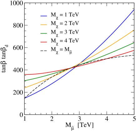
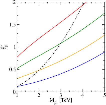
Figure 1: Left: Values of the product $\tan\beta\tan\beta_{d}$ that result in $\Delta a_{\mu}^{\rm{\scriptscriptstyle FSSM}}=251\times 10^{-11}$, as a function of the smuon mass and for different values of a common mass for higgsinos and EW gauginos. Right: Values of the loop-corrected muon Yukawa coupling of the FSSM that correspond to the solution for $\tan\beta\tan\beta_{d}$ shown in the left plot. The meaning of the lines is the same as in the left plot.

To set the stage for our discussion, in the left plot of figure 1 we show the values of $\tan\beta\tan\beta_{d}=v_{u}/v_{d^{\prime}}$ that result in the desired smuon-higgsino-gaugino contribution to $a_{\mu}$, as a function of the common smuon mass $M_{\tilde{\mu}}$ and for different values of $M_{\chi}$. In particular, the blue, yellow, green and red solid lines correspond to gaugino and higgsino masses of $1,2,3$ and $4$ TeV, respectively, while the black dashed line corresponds to the choice $M_{\chi}=M_{\tilde{\mu}}$. The EW gauge couplings entering eqs. (28) and (31) are evaluated at the scale $Q=M_{\tilde{\mu}}$, but we found qualitatively similar results for any choice of scale in the few-TeV range. The plot shows that the values of $\tan\beta\tan\beta_{d}$ necessary to obtain $\Delta a_{\mu}^{\rm{\scriptscriptstyle FSSM}}=251\times 10^{-11}$ are typically in the few-hundreds range, and can reach as much as $940$ for the largest considered value of $M_{\tilde{\mu}}$.

In the right plot of figure 1 we show instead the values of the loop-corrected muon Yukawa coupling of the FSSM at the scale $Q=M_{\tilde{\mu}}$,

$$\hat{y}^{\prime}_{\mu}(M_{\tilde{\mu}})~{}=~{}\frac{g_{\mu}(M_{\tilde{\mu}})/(\cos\tilde{\beta}\cos\beta_{d})}{1+\epsilon_{\ell}\,\tan\beta\tan\beta_{d}}~{},$$ (33)

that correspond to the solutions for $\tan\beta\tan\beta_{d}$ shown in the left plot. The FSSM coupling $\hat{y}^{\prime}_{\mu}$ controls the higgsino-muon-smuon and Higgs-smuon-smuon interactions involved in the smuon-higgsino-gaugino contributions to $a_{\mu}$, as well as the Higgs-smuon-smuon interaction involved in the smuon contribution to the quartic Higgs coupling. The solid and dashed lines have the same meaning as in the left plot. We set $\tan\beta_{u}=100$ in order to determine the angle $\tilde{\beta}$ entering eq. (33), but the results are essentially independent of this choice as long as $\tan\beta_{u}\gg 1$. The plot shows that larger values of $\hat{y}^{\prime}_{\mu}$ are required to obtain the desired contribution to $a_{\mu}$ when the smuon mass increases, due to the $M_{\tilde{\mu}}^{-2}$ suppression in eq. (28). Also, for a fixed value of the smuon mass, larger values of $\hat{y}^{\prime}_{\mu}$ are required when $M_{\chi}$ increases. We remark that, while the considered values of $\hat{y}^{\prime}_{\mu}(M_{\tilde{\mu}})$ are all perturbative, further constraints on this scenario could arise if we required that $\hat{y}^{\prime}_{\mu}$ remain perturbative all the way up to the GUT scale.

In the presence of a large muon Yukawa coupling, the smuon contribution to the quartic Higgs coupling in eq. (26) is dominated by a negative term

$$(4\pi)^{2}\,\Delta\lambda^{\tilde{\mu}}~{}\approx~{}-\frac{\hat{y}_{\mu}^{\prime\,4}}{6}\,\left(\frac{M_{\chi}}{M_{\tilde{\mu}}}\right)^{4},$$ (34)

and can become substantial. An increased positive contribution from loops involving the remaining SUSY particles is then needed to satisfy the constraint arising from the measured value of the Higgs mass. As mentioned in the previous section, such positive contribution can most easily come from the stops, which themselves have generally large couplings to the SM-like Higgs boson.

In figure 2 we plot the values of the common stop mass $M_{\tilde{t}}$ that are required to obtain the correct prediction for the quartic Higgs coupling in FSSM scenarios where the smuon-higgsino-gaugino loops provide the desired contribution to $(g-2)_{\mu}$. We set the matching scale $Q$ in eqs. (20) and (23)–(25) equal to the stop mass, as this ensures a full NNL resummation of the large logarithmic corrections controlled by the top Yukawa coupling. All of the running couplings entering our calculation are then computed at the scale $Q=M_{\tilde{t}}$. The common mass parameters for the smuons, $M_{\tilde{\mu}}$, and for higgsinos and EW gauginos, $M_{\chi}$, are varied as in figure 1 (note that we add a purple solid line for $M_{\chi}=3.5$ TeV). We fix $\tan\tilde{\beta}=20$, thus ensuring that the tree-level prediction for $\lambda_{{\rm{\scriptscriptstyle SM}}}$ in eq. (20) is essentially saturated, and $\tan\beta_{u}=100$ (the latter choice has little impact on our results as long as $\tan\beta_{u}\gg 1$). In contrast, $\tan\beta_{d}$ is computed in each point from the requirement that $\Delta a_{\mu}^{\rm{\scriptscriptstyle FSSM}}=251\times 10^{-11}$. The stop mixing parameter is fixed to the value $X_{t}=\sqrt{6}\,M_{\tilde{t}}\,$ that maximizes the one-loop stop contribution to the quartic Higgs coupling, see eq. (27). Our choices for $\tan\tilde{\beta}$ and $X_{t}$ ensure that the values of the stop mass shown in figure 2 are about the minimal ones that provide the correct prediction for the Higgs mass (in other words, different choices for these parameters would result in an overall upward shift of all lines in the figure). For the remaining free parameters of our simplified FSSM scenario we choose $M_{H}=M_{3}=M_{\chi}$. The choice of the common mass parameter for the heavy Higgs doublets has only a small impact on our results, because the corresponding contributions to the quartic Higgs coupling, see eq. (24), all involve four powers of the EW gauge couplings. The choice of the gluino mass affects our calculation only through the corrections to the quark Yukawa couplings in eqs. (17) and (18), and its qualitative impact on our results is generally not substantial. Our choice of a positive value for the ratio $X_{t}/M_{3}$ enhances the loop-corrected top Yukawa coupling $\hat{y}_{t}$, whereas a negative value would suppress it and require somewhat heavier stops in order to satisfy the Higgs-mass constraint. However, we recall that, for positive values of $X_{s}/M_{3}$ (i.e., negative values of $\mu_{ud^{\prime}}/M_{3}$), a fine-tuned choice of parameters such that $\Delta g_{s}\simeq 1$ might lead the strange Yukawa coupling to blow up, resulting in a large negative strange-squark contribution to the quartic Higgs coupling.

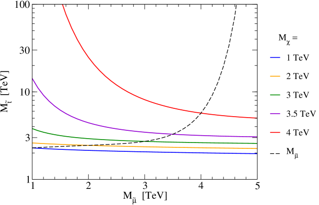
Figure 2: Values of the stop mass $M_{\tilde{t}}$ that result in the correct prediction for the Higgs mass when $\tan\beta_{d}$ is fixed by the requirement that the smuon-higgsino-gaugino contribution solve the $(g-2)_{\mu}$ anomaly, as a function of the smuon mass $M_{\tilde{\mu}}$ and for different values of the common higgsino/gaugino mass $M_{\chi}$. The remaining free parameters of our simplified FSSM scenario are fixed as $\tan\tilde{\beta}=20$, $\tan\beta_{u}=100$, $X_{t}=\sqrt{6}\,M_{\tilde{t}}$ and $M_{H}=M_{3}=M_{\chi}$.

Figure 2 shows that there are regions of the FSSM parameter space in which the interplay between the requirements of a suitable contribution to $a_{\mu}$ and of a correct prediction for the quartic Higgs coupling implies a strongly hierarchical SUSY spectrum, with the stops being significantly heavier than smuons, higgsinos and EW gauginos. Unsurprisingly, in the scenario with $M_{\chi}=M_{\tilde{\mu}}$ (the black dashed line) this happens for the largest values of $M_{\tilde{\mu}}$, when a large muon Yukawa coupling $\hat{y}^{\prime}_{\mu}$ is needed to counteract the $M_{\tilde{\mu}}^{-2}$ suppression of the smuon-higgsino-gaugino contribution to $a_{\mu}$, see eq. (28), and results in a large negative contribution to the quartic Higgs coupling, see eq. (34). Moreover, the left ends of the red, purple and (to a lesser extent) green lines show that very heavy stops may be needed also at lower values of $M_{\tilde{\mu}}$ – where figure 1 shows that $\hat{y}^{\prime}_{\mu}\lesssim 1$ is sufficient for the solution of the $(g-2)_{\mu}$ anomaly – if the smuon contribution to the quartic Higgs coupling in eq. (34) is enhanced by a large ratio $M_{\chi}/M_{\tilde{\mu}}$. Even in regions of the parameter space where the SUSY spectrum is not strongly hierarchical, such as the right end of the red line in figure 2, the minimal value of $M_{\tilde{t}}$ required to obtain the correct Higgs-mass prediction can be significantly higher than the $2\!-\!3$ TeV typically found in the MSSM. Finally, we find that for $M_{\chi}\lesssim 2$ TeV (the yellow and blue lines) the smuon contribution to the quartic Higgs coupling never becomes substantial in our simplified scenario: at low $M_{\tilde{\mu}}$ – where the desired contribution to $(g-2)_{\mu}$ is obtained with $\hat{y}^{\prime}_{\mu}\lesssim 0.5$ – there is little or no enhancement from the $(M_{\chi}/M_{\tilde{\mu}})^{4}$ term in eq. (34), whereas at high $M_{\tilde{\mu}}$ the corresponding suppression wins over the enhancement of $\hat{y}^{\prime}_{\mu}$. The mild residual dependence of the yellow and blue lines on $M_{\tilde{\mu}}$ and $M_{\chi}$ stems from the terms controlled by the EW gauge couplings in eqs. (23)–(25).

We remark that in our simplified FSSM scenario, where $M_{\chi}\equiv M_{1}=M_{2}=\mu=\tilde{\mu}$ , the condition $M_{\chi}/M_{\tilde{\mu}}>1$ implies that the LSP is a heavy sneutrino, which is generally disfavored by Dark Matter considerations [55, 56]. While a detailed study of Dark Matter constraints on the FSSM parameter space is beyond the scope of our paper, using the general formula for $\Delta\lambda^{\chi}$ we verified that very heavy stops may be required even in scenarios where the LSP is always an EW gaugino. In particular, if we fix $M_{1}=1$ TeV and $M_{\chi}\equiv M_{2}=\mu=\tilde{\mu}$ we still find a rise in the stop mass similar to the black dashed line in figure 2 for $M_{\tilde{\mu}}=M_{\chi}\,\gtrsim\,4$ TeV. However, we no longer see the rise at low $M_{\tilde{\mu}}$ in the lines corresponding to larger $M_{\chi}$, because in this region the desired contribution to $(g-2)_{\mu}$ is obtained with lower values of $\hat{y}^{\prime}_{\mu}$ than in the case of degenerate gaugino masses.

It is interesting to note that, in contrast to what we find for the FSSM, in the MSSM the combination of the constraints from the Higgs-mass prediction and from $(g-2)_{\mu}$ can yield upper bounds on the stop masses, see e.g. ref. [57]. Indeed, in the absence of large and negative contributions from other sectors, a large and positive contribution from heavy-stop loops to the prediction for $\lambda_{{\rm{\scriptscriptstyle SM}}}$ must be compensated for by a suppression of the tree-level prediction via a lower value of $\tan\beta$. However, in the MSSM this would also suppress the smuon-higgsino-gaugino contribution to $a_{\mu}$, jeopardizing the solution of the $(g-2)_{\mu}$ anomaly. The interplay of the two constraints is different in the FSSM, because in this model the ratio of vevs that determines the tree-level prediction for $\lambda_{{\rm{\scriptscriptstyle SM}}}$ can be varied independently of the ratio of vevs that enhances the smuon-higgsino-gaugino contribution to $a_{\mu}$.

Finally, we remark that, when the stops are an order of magnitude (or more) heavier than the other SUSY particles, our calculation of the Higgs mass loses accuracy, and we would need to build a two-step EFT setup in which the stops are separately integrated out of the FSSM at a scale comparable with their mass. However, the aim of our study is not a precise determination of masses that, for the time being, are beyond experimental reach, but rather a qualitative insight on the structure of this heavy-SUSY model. The possibility of a hierarchical mass spectrum has obvious implications for the prospects of probing the FSSM at future colliders, and from the model-building point of view it might also complicate any attempt to devise a suitable mechanism of SUSY breaking.

5 Conclusions

A scenario for particle physics that is now looking increasingly plausible is the one where new physics manifests itself in one or more deviations from the SM predictions for rare processes or precision observables, but the BSM particles responsible for those deviations are too heavy to be discovered at the LHC. In this case, all possible clues should be exploited to unravel the structure of the heavy BSM sector, also to guide the searches for the new particles at future colliders. If a model that aims to explain the observed anomalies is supersymmetric, it will generally involve a prediction for the quartic coupling $\lambda_{{\rm{\scriptscriptstyle SM}}}$ of the SM-like Higgs boson. Since all of the new particles in the SUSY model affect $\lambda_{{\rm{\scriptscriptstyle SM}}}$ through radiative corrections, its prediction can reveal correlations between the sectors of the model that are involved in the observed anomalies and those that are not.

In this paper we studied the Higgs-mass constraints on the parameter space of a supersymmetric four-Higgs-doublet model, the FSSM [37], which was recently proposed as a solution of the $(g-2)_{\mu}$ anomaly [10, 11] with SUSY particle masses beyond the current reach of the LHC. We followed the modern approach of taking $M_{h}$ as an input rather than an output of our calculation, and we relied on an EFT setup to account at the NLL order for the large logarithmic corrections to the relation between the measured value of $M_{h}$ and the value of $\lambda_{{\rm{\scriptscriptstyle SM}}}$ at the SUSY scale. In our one-loop calculation of the prediction for $\lambda_{{\rm{\scriptscriptstyle SM}}}$ we adapted to the case of the FSSM the results derived in ref. [39] for a general renormalizable theory. We provided explicit formulas for the one-loop correction to the quartic Higgs coupling in a simplified FSSM scenario, but we make the result for the general FSSM available on request in electronic form.

We found that the prediction for $\lambda_{{\rm{\scriptscriptstyle SM}}}$ establishes interesting relations between the parameters that contribute to $(g-2)_{\mu}$, namely the masses of smuons, higgsinos and EW gauginos, and the parameters in the stop sector. In particular, there are scenarios with a suitable SUSY contribution to $(g-2)_{\mu}$ in which the stops need to be considerably heavier than smuons, higgsinos and EW gauginos, in order to compensate for a large and negative smuon contribution to the prediction for $\lambda_{{\rm{\scriptscriptstyle SM}}}$. The possibility of a hierarchical SUSY mass spectrum should be taken into account when assessing the prospects of probing the FSSM at future colliders.

As mentioned in ref. [37], further investigations of the FSSM could address the flavor structure of the quark sector, in which case the large corrections to the strange Yukawa coupling discussed in section 3 of our paper would need to be taken into account. Other directions of investigation could address the extended Higgs sector of the FSSM, exploring e.g. the collider phenomenology of the heavy Higgs bosons, or the stability of the scalar potential. With the present study, we aimed to provide a proof of concept – applicable also to other models and other anomalies – of how the Higgs-mass prediction can be used, in combination with other observables, to shed some light on the hidden structure of a SUSY model with heavy superparticles.

Appendix

We provide here explicit formulas for the tree-level mass matrices of the Higgs bosons in the FSSM. In the Higgs basis, we decompose the four SU(2) doublets (all with positive hypercharge) as

$$\Phi_{h}~{}=\,\left(\!\begin{array}[]{c}G^{+}\\ v+\frac{1}{\sqrt{2}}(h+i\,G^{0})\end{array}\!\right),~{}~{}~{}~{}~{}\Phi_{H}~{}=\,\left(\!\begin{array}[]{c}H^{+}\\ \frac{1}{\sqrt{2}}(H+i\,A)\end{array}\!\right),~{}~{}~{}~{}~{}\Phi^{\prime}_{d,u}~{}=\,\left(\!\begin{array}[]{c}\phi^{\prime\,+}_{d,u}\\ \frac{1}{\sqrt{2}}(\phi^{\prime}_{d,u}+i\,a^{\prime}_{d,u})\end{array}\!\right).$$ (A1)

In this basis the mass matrices for the scalar $(h,\,H,\,\phi^{\prime}_{d},\,\phi^{\prime}_{u})$, pseudoscalar $(G^{0},\,A,\,a^{\prime}_{d},\,a^{\prime}_{u})$ and charged $(G^{+},\,H^{+},\,\phi^{\prime\,+}_{d},\,\phi^{\prime\,+}_{u})$ components of the four doublets read

$${\cal M}^{2}_{S}~{}=~{}\left(\!\begin{array}[]{cccc}M_{\scriptscriptstyle Z}^{2}\,\cos^{2}2\tilde{\beta}&-\frac{1}{2}\,M_{\scriptscriptstyle Z}^{2}\,\sin 4\tilde{\beta}&0&0\\[2.84526pt] -\frac{1}{2}\,M_{\scriptscriptstyle Z}^{2}\,\sin 4\tilde{\beta}&M_{\scriptscriptstyle Z}^{2}\,\sin^{2}2\tilde{\beta}+2\,b_{12}/\sin 2\tilde{\beta}&-b_{32}/\cos\tilde{\beta}&b_{14}/\sin\tilde{\beta}\\[2.84526pt] 0&-b_{32}/\cos\tilde{\beta}&M_{\Phi_{d}^{\prime}}^{2}+\frac{1}{2}\,M_{\scriptscriptstyle Z}^{2}\,\cos 2\tilde{\beta}&-b_{34}\\[2.84526pt] 0&b_{14}/\sin\tilde{\beta}&-b_{34}&M_{\Phi_{u}^{\prime}}^{2}-\frac{1}{2}\,M_{\scriptscriptstyle Z}^{2}\,\cos 2\tilde{\beta}\end{array}\!\right),$$ (A2)

$${\cal M}^{2}_{P}~{}=~{}\left(\!\begin{array}[]{cccc}0&0&0&0\\[2.84526pt] 0&2\,b_{12}/\sin 2\tilde{\beta}&-b_{32}/\cos\tilde{\beta}&b_{14}/\sin\tilde{\beta}\\[2.84526pt] 0&-b_{32}/\cos\tilde{\beta}&M_{\Phi_{d}^{\prime}}^{2}+\frac{1}{2}\,M_{\scriptscriptstyle Z}^{2}\,\cos 2\tilde{\beta}&-b_{34}\\[2.84526pt] 0&b_{14}/\sin\tilde{\beta}&-b_{34}&M_{\Phi_{u}^{\prime}}^{2}-\frac{1}{2}\,M_{\scriptscriptstyle Z}^{2}\,\cos 2\tilde{\beta}\end{array}\!\right),$$ (A3)

$${\cal M}^{2}_{\pm}~{}=~{}\left(\!\begin{array}[]{cccc}0&0&0&0\\[2.84526pt] 0&M_{\scriptscriptstyle W}^{2}+2\,b_{12}/\sin 2\tilde{\beta}&-b_{32}/\cos\tilde{\beta}&b_{14}/\sin\tilde{\beta}\\[2.84526pt] 0&-b_{32}/\cos\tilde{\beta}&M_{\Phi_{d}^{\prime}}^{2}-\left(M_{\scriptscriptstyle W}^{2}-\frac{1}{2}\,M_{\scriptscriptstyle Z}^{2}\right)\,\cos 2\tilde{\beta}&-b_{34}\\[2.84526pt] 0&b_{14}/\sin\tilde{\beta}&-b_{34}&M_{\Phi_{u}^{\prime}}^{2}+\left(M_{\scriptscriptstyle W}^{2}-\frac{1}{2}\,M_{\scriptscriptstyle Z}^{2}\right)\,\cos 2\tilde{\beta}\end{array}\!\right),$$ (A4)

where the mass parameters $M_{\Phi_{d,u}^{\prime}}^{2}$ and the mixing parameters  $b_{ij}$ are combinations of the original mass parameters and $B$-terms as defined in eqs. (1) and (4):

$$M_{\Phi_{d}^{\prime}}^{2} = \left(m_{dd}^{2}+\mu_{ud}^{2}+\mu_{u^{\prime}\!d}^{2}\right)\cos^{2}\beta_{d}~{}+~{}\left(m_{d^{\prime}\!d^{\prime}}^{2}+\mu_{u^{\prime}\!d^{\prime}}^{2}+\mu_{ud^{\prime}}^{2}\right)\sin^{2}\beta_{d}$$ (A5)

$$-\left(m^{2}_{dd^{\prime}}+\mu_{ud}\mu_{ud^{\prime}}+\mu_{u^{\prime}\!d^{\prime}}\mu_{u^{\prime}\!d}\right)\sin 2\beta_{d}~{},$$

$$M_{\Phi_{u}^{\prime}}^{2} = \left(m_{uu}^{2}+\mu_{ud}^{2}+\mu_{ud^{\prime}}^{2}\right)\cos^{2}\beta_{u}~{}+~{}\left(m_{u^{\prime}\!u^{\prime}}^{2}+\mu_{u^{\prime}\!d^{\prime}}^{2}+\mu_{u^{\prime}\!d}^{2}\right)\sin^{2}\beta_{u}$$ (A6)

$$-\left(m^{2}_{uu^{\prime}}+\mu_{ud}\mu_{u^{\prime}\!d}+\mu_{u^{\prime}\!d^{\prime}}\mu_{ud^{\prime}}\right)\sin 2\beta_{u}~{},$$

$$b_{12} = \sin\beta_{d}\,\left(B_{ud}\sin\beta_{u}+B_{u^{\prime}\!d}\cos\beta_{u}\right)~{}+~{}\cos\beta_{d}\,\left(B_{ud^{\prime}}\sin\beta_{u}+B_{u^{\prime}\!d^{\prime}}\cos\beta_{u}\right)~{},$$ (A7)

$$b_{32} = \cos\beta_{d}\,\left(B_{ud}\sin\beta_{u}+B_{u^{\prime}\!d}\cos\beta_{u}\right)~{}-~{}\sin\beta_{d}\,\left(B_{ud^{\prime}}\sin\beta_{u}+B_{u^{\prime}\!d^{\prime}}\cos\beta_{u}\right)~{},$$ (A8)

$$b_{14} = \sin\beta_{d}\,\left(B_{ud}\cos\beta_{u}-B_{u^{\prime}\!d}\sin\beta_{u}\right)~{}+~{}\cos\beta_{d}\,\left(B_{ud^{\prime}}\cos\beta_{u}-B_{u^{\prime}\!d^{\prime}}\sin\beta_{u}\right)~{},$$ (A9)

$$b_{34} = \cos\beta_{d}\,\left(B_{ud}\cos\beta_{u}-B_{u^{\prime}\!d}\sin\beta_{u}\right)~{}-~{}\sin\beta_{d}\,\left(B_{ud^{\prime}}\cos\beta_{u}-B_{u^{\prime}\!d^{\prime}}\sin\beta_{u}\right)~{}.$$ (A10)

The minimum conditions of the Higgs potential have been used to remove four combinations of the original parameters from eqs. (A2)–(A4). In the limit of unbroken EW symmetry (i.e., $v\rightarrow 0$), which we adopt in the calculation of the matching condition for the quartic coupling of the SM-like Higgs, the mixing between the SM-like scalar $h$ and the three heavy scalars vanishes, and the $3\!\times\!3$ sub-matrices for the masses of the scalar, pseudoscalar and charged components of the heavy doublets $\Phi_{H}$, $\Phi^{\prime}_{d}$ and $\Phi^{\prime}_{u}$ all reduce to:

$${\cal M}^{2}_{H}~{}=~{}\left(\!\begin{array}[]{ccc}2\,b_{12}/\sin 2\tilde{\beta}&-b_{32}/\cos\tilde{\beta}&b_{14}/\sin\tilde{\beta}\\[2.84526pt] -b_{32}/\cos\tilde{\beta}&M_{\Phi_{d}^{\prime}}^{2}&-b_{34}\\[2.84526pt] b_{14}/\sin\tilde{\beta}&-b_{34}&M_{\Phi_{u}^{\prime}}^{2}\end{array}\!\right).$$ (A11)

We can then introduce a $3\!\times\!3$ orthogonal matrix $R_{H}$ that rotates the three heavy doublets of the Higgs basis into a basis of mass eigenstates:

$$\left(\!\begin{array}[]{c}H_{1}\\ H_{2}\\ H_{3}\end{array}\!\right)~{}=~{}R_{H}\,\left(\!\begin{array}[]{c}\Phi_{\scriptscriptstyle H}\\ \Phi_{d}^{\prime}\\ \Phi_{u}^{\prime}\end{array}\!\right)~{},~{}~{}~{}~{}~{}~{}~{}~{}~{}~{}~{}{\rm diag}\left(M_{H_{1}}^{2},M_{H_{2}}^{2},M_{H_{3}}^{2}\right)~{}=~{}R_{H}\,{\cal M}^{2}_{H}\,R_{H}^{T}~{}.$$ (A12)

References

- [1] CMS Collaboration, S. Chatrchyan et al., Observation of a New Boson at a Mass of 125 GeV with the CMS Experiment at the LHC. Phys. Lett. B 716 (2012) 30–61, arXiv:1207.7235 [hep-ex].
- [2] ATLAS Collaboration, G. Aad et al., Observation of a new particle in the search for the Standard Model Higgs boson with the ATLAS detector at the LHC. Phys. Lett. B 716 (2012) 1–29, arXiv:1207.7214 [hep-ex].
- [3] ATLAS, CMS Collaboration, G. Aad et al., Combined Measurement of the Higgs Boson Mass in Collisions at and 8 TeV with the ATLAS and CMS Experiments. Phys. Rev. Lett. 114 (2015) 191803, arXiv:1503.07589 [hep-ex].
- [4] ATLAS, CMS Collaboration, G. Aad et al., Measurements of the Higgs boson production and decay rates and constraints on its couplings from a combined ATLAS and CMS analysis of the LHC pp collision data at and 8 TeV. JHEP 08 (2016) 045, arXiv:1606.02266 [hep-ex].
- [5] P. Slavich et al., Higgs-mass predictions in the MSSM and beyond. Eur. Phys. J. C 81 (2021) no. 5, 450, arXiv:2012.15629 [hep-ph].
- [6] LHCb Collaboration, R. Aaij et al., Test of lepton universality using decays. Phys. Rev. Lett. 113 (2014) 151601, arXiv:1406.6482 [hep-ex].
- [7] LHCb Collaboration, R. Aaij et al., Test of lepton universality with decays. JHEP 08 (2017) 055, arXiv:1705.05802 [hep-ex].
- [8] LHCb Collaboration, R. Aaij et al., Search for lepton-universality violation in decays. Phys. Rev. Lett. 122 (2019) no. 19, 191801, arXiv:1903.09252 [hep-ex].
- [9] LHCb Collaboration, R. Aaij et al., Test of lepton universality in beauty-quark decays. arXiv:2103.11769 [hep-ex].
- [10] Muon g-2 Collaboration, B. Abi et al., Measurement of the Positive Muon Anomalous Magnetic Moment to 0.46 ppm. Phys. Rev. Lett. 126 (2021) no. 14, 141801, arXiv:2104.03281 [hep-ex].
- [11] Muon g-2 Collaboration, G. W. Bennett et al., Final Report of the Muon E821 Anomalous Magnetic Moment Measurement at BNL. Phys. Rev. D 73 (2006) 072003, arXiv:hep-ex/0602035.
- [12] T. Aoyama et al., The anomalous magnetic moment of the muon in the Standard Model. Phys. Rept. 887 (2020) 1–166, arXiv:2006.04822 [hep-ph].
- [13] T. Aoyama, M. Hayakawa, T. Kinoshita, and M. Nio, Complete Tenth-Order QED Contribution to the Muon g-2. Phys. Rev. Lett. 109 (2012) 111808, arXiv:1205.5370 [hep-ph].
- [14] T. Aoyama, T. Kinoshita, and M. Nio, Theory of the Anomalous Magnetic Moment of the Electron. Atoms 7 (2019) no. 1, 28.
- [15] A. Czarnecki, W. J. Marciano, and A. Vainshtein, Refinements in electroweak contributions to the muon anomalous magnetic moment. Phys. Rev. D 67 (2003) 073006, arXiv:hep-ph/0212229. [Erratum: Phys.Rev.D 73, 119901 (2006)].
- [16] C. Gnendiger, D. Stöckinger, and H. Stöckinger-Kim, The electroweak contributions to after the Higgs boson mass measurement. Phys. Rev. D 88 (2013) 053005, arXiv:1306.5546 [hep-ph].
- [17] M. Davier, A. Hoecker, B. Malaescu, and Z. Zhang, Reevaluation of the hadronic vacuum polarisation contributions to the Standard Model predictions of the muon and using newest hadronic cross-section data. Eur. Phys. J. C 77 (2017) no. 12, 827, arXiv:1706.09436 [hep-ph].
- [18] A. Keshavarzi, D. Nomura, and T. Teubner, Muon and : a new data-based analysis. Phys. Rev. D 97 (2018) no. 11, 114025, arXiv:1802.02995 [hep-ph].
- [19] G. Colangelo, M. Hoferichter, and P. Stoffer, Two-pion contribution to hadronic vacuum polarization. JHEP 02 (2019) 006, arXiv:1810.00007 [hep-ph].
- [20] M. Hoferichter, B.-L. Hoid, and B. Kubis, Three-pion contribution to hadronic vacuum polarization. JHEP 08 (2019) 137, arXiv:1907.01556 [hep-ph].
- [21] M. Davier, A. Hoecker, B. Malaescu, and Z. Zhang, A new evaluation of the hadronic vacuum polarisation contributions to the muon anomalous magnetic moment and to . Eur. Phys. J. C 80 (2020) no. 3, 241, arXiv:1908.00921 [hep-ph]. [Erratum: Eur.Phys.J.C 80, 410 (2020)].
- [22] A. Keshavarzi, D. Nomura, and T. Teubner, of charged leptons, , and the hyperfine splitting of muonium. Phys. Rev. D 101 (2020) no. 1, 014029, arXiv:1911.00367 [hep-ph].
- [23] A. Kurz, T. Liu, P. Marquard, and M. Steinhauser, Hadronic contribution to the muon anomalous magnetic moment to next-to-next-to-leading order. Phys. Lett. B 734 (2014) 144–147, arXiv:1403.6400 [hep-ph].
- [24] K. Melnikov and A. Vainshtein, Hadronic light-by-light scattering contribution to the muon anomalous magnetic moment revisited. Phys. Rev. D 70 (2004) 113006, arXiv:hep-ph/0312226.
- [25] P. Masjuan and P. Sanchez-Puertas, Pseudoscalar-pole contribution to the : a rational approach. Phys. Rev. D 95 (2017) no. 5, 054026, arXiv:1701.05829 [hep-ph].
- [26] G. Colangelo, M. Hoferichter, M. Procura, and P. Stoffer, Dispersion relation for hadronic light-by-light scattering: two-pion contributions. JHEP 04 (2017) 161, arXiv:1702.07347 [hep-ph].
- [27] M. Hoferichter, B.-L. Hoid, B. Kubis, S. Leupold, and S. P. Schneider, Dispersion relation for hadronic light-by-light scattering: pion pole. JHEP 10 (2018) 141, arXiv:1808.04823 [hep-ph].
- [28] A. Gérardin, H. B. Meyer, and A. Nyffeler, Lattice calculation of the pion transition form factor with Wilson quarks. Phys. Rev. D 100 (2019) no. 3, 034520, arXiv:1903.09471 [hep-lat].
- [29] J. Bijnens, N. Hermansson-Truedsson, and A. Rodríguez-Sánchez, Short-distance constraints for the HLbL contribution to the muon anomalous magnetic moment. Phys. Lett. B 798 (2019) 134994, arXiv:1908.03331 [hep-ph].
- [30] G. Colangelo, F. Hagelstein, M. Hoferichter, L. Laub, and P. Stoffer, Longitudinal short-distance constraints for the hadronic light-by-light contribution to with large- Regge models. JHEP 03 (2020) 101, arXiv:1910.13432 [hep-ph].
- [31] T. Blum, N. Christ, M. Hayakawa, T. Izubuchi, L. Jin, C. Jung, and C. Lehner, Hadronic Light-by-Light Scattering Contribution to the Muon Anomalous Magnetic Moment from Lattice QCD. Phys. Rev. Lett. 124 (2020) no. 13, 132002, arXiv:1911.08123 [hep-lat].
- [32] G. Colangelo, M. Hoferichter, A. Nyffeler, M. Passera, and P. Stoffer, Remarks on higher-order hadronic corrections to the muon g2. Phys. Lett. B 735 (2014) 90–91, arXiv:1403.7512 [hep-ph].
- [33] W. Altmannshofer and D. M. Straub, Viability of MSSM scenarios at very large . JHEP 09 (2010) 078, arXiv:1004.1993 [hep-ph].
- [34] M. Chakraborti, S. Heinemeyer, and I. Saha, The new “MUON G-2” result and supersymmetry. Eur. Phys. J. C 81 (2021) no. 12, 1114, arXiv:2104.03287 [hep-ph].
- [35] P. Athron, C. Balázs, D. H. Jacob, W. Kotlarski, D. Stöckinger, and H. Stöckinger-Kim, New physics explanations of in light of the FNAL muon measurement. JHEP 09 (2021) 080, arXiv:2104.03691 [hep-ph].
- [36] M. Bach, J.-h. Park, D. Stöckinger, and H. Stöckinger-Kim, Large muon with TeV-scale SUSY masses for . JHEP 10 (2015) 026, arXiv:1504.05500 [hep-ph].
- [37] W. Altmannshofer, S. A. Gadam, S. Gori, and N. Hamer, Explaining with Multi-TeV Sleptons. JHEP 07 (2021) 118, arXiv:2104.08293 [hep-ph].
- [38] K. Benakli, L. Darmé, M. D. Goodsell, and P. Slavich, A Fake Split Supersymmetry Model for the 126 GeV Higgs. JHEP 05 (2014) 113, arXiv:1312.5220 [hep-ph].
- [39] J. Braathen, M. D. Goodsell, and P. Slavich, Matching renormalisable couplings: simple schemes and a plot. Eur. Phys. J. C 79 (2019) no. 8, 669, arXiv:1810.09388 [hep-ph].
- [40] N. Escudero, C. Munoz, and A. M. Teixeira, FCNCs in supersymmetric multi-Higgs doublet models. Phys. Rev. D 73 (2006) 055015, arXiv:hep-ph/0512046.
- [41] B. A. Kniehl, A. F. Pikelner, and O. L. Veretin, mr: a C++ library for the matching and running of the Standard Model parameters. Comput. Phys. Commun. 206 (2016) 84–96, arXiv:1601.08143 [hep-ph].
- [42] B. A. Kniehl, A. F. Pikelner, and O. L. Veretin, Two-loop electroweak threshold corrections in the Standard Model. Nucl. Phys. B 896 (2015) 19–51, arXiv:1503.02138 [hep-ph].
- [43] Particle Data Group Collaboration, P. A. Zyla et al., Review of Particle Physics. PTEP 2020 (2020) no. 8, 083C01.
- [44] R. Hempfling and B. A. Kniehl, On the relation between the fermion pole mass and MS Yukawa coupling in the standard model. Phys. Rev. D 51 (1995) 1386–1394, arXiv:hep-ph/9408313.
- [45] G. Degrassi, P. Gambino, and P. Slavich, SusyBSG: A Fortran code for BR[B — X(s) gamma] in the MSSM with Minimal Flavor Violation. Comput. Phys. Commun. 179 (2008) 759–771, arXiv:0712.3265 [hep-ph].
- [46] A. V. Bednyakov, A. F. Pikelner, and V. N. Velizhanin, Anomalous dimensions of gauge fields and gauge coupling beta-functions in the Standard Model at three loops. JHEP 01 (2013) 017, arXiv:1210.6873 [hep-ph].
- [47] A. V. Bednyakov, A. F. Pikelner, and V. N. Velizhanin, Yukawa coupling beta-functions in the Standard Model at three loops. Phys. Lett. B 722 (2013) 336–340, arXiv:1212.6829 [hep-ph].
- [48] A. V. Bednyakov, A. F. Pikelner, and V. N. Velizhanin, Higgs self-coupling beta-function in the Standard Model at three loops. Nucl. Phys. B 875 (2013) 552–565, arXiv:1303.4364 [hep-ph].
- [49] M.-x. Luo and Y. Xiao, Two loop renormalization group equations in the standard model. Phys. Rev. Lett. 90 (2003) 011601, arXiv:hep-ph/0207271.
- [50] E. Bagnaschi, G. F. Giudice, P. Slavich, and A. Strumia, Higgs Mass and Unnatural Supersymmetry. JHEP 09 (2014) 092, arXiv:1407.4081 [hep-ph].
- [51] T. Kwasnitza, D. Stöckinger, and A. Voigt, Improved MSSM Higgs mass calculation using the 3-loop FlexibleEFTHiggs approach including -resummation. JHEP 07 (2020) no. 07, 197, arXiv:2003.04639 [hep-ph].
- [52] T. Kwasnitza and D. Stöckinger, Resummation of terms enhanced by trilinear squark-Higgs couplings in the MSSM. JHEP 08 (2021) 070, arXiv:2103.08616 [hep-ph].
- [53] B. C. Allanach, G. Hiller, D. R. T. Jones, and P. Slavich, Flavour Violation in Anomaly Mediated Supersymmetry Breaking. JHEP 04 (2009) 088, arXiv:0902.4880 [hep-ph].
- [54] E. Bagnaschi, J. Pardo Vega, and P. Slavich, Improved determination of the Higgs mass in the MSSM with heavy superpartners. Eur. Phys. J. C 77 (2017) no. 5, 334, arXiv:1703.08166 [hep-ph].
- [55] T. Falk, K. A. Olive, and M. Srednicki, Heavy sneutrinos as dark matter. Phys. Lett. B 339 (1994) 248–251, arXiv:hep-ph/9409270.
- [56] C. Arina and N. Fornengo, Sneutrino cold dark matter, a new analysis: Relic abundance and detection rates. JHEP 11 (2007) 029, arXiv:0709.4477 [hep-ph].
- [57] M. Badziak, Z. Lalak, M. Lewicki, M. Olechowski, and S. Pokorski, Upper bounds on sparticle masses from muon g 2 and the Higgs mass and the complementarity of future colliders. JHEP 03 (2015) 003, arXiv:1411.1450 [hep-ph].