Exclusive determinations of $|V_{cb}|$ and $R(D^{*})$ through unitarity

Abstract

In this work we apply the Dispersive Matrix (DM) method of Refs. DiCarlo:2021dzg ; Martinelli:2021onb to the lattice computations of the Form Factors (FFs) entering the semileptonic $B\to D^{*}\ell\nu_{\ell}$ decays, recently produced by the FNAL/MILC Collaborations FermilabLattice:2021cdg at small, but non-vanishing values of the recoil variable ($w-1$). Thanks to the DM method we obtain the FFs in the whole kinematical range accessible to the decay in a completely model-independent and non-perturbative way, implementing exactly both unitarity and kinematical constraints. Using our theoretical bands of the FFs we extract $|V_{cb}|$ from the experimental data and compute the theoretical value of $R(D^{*})$. Our final result for $|V_{cb}|$ reads $|V_{cb}|=(41.3\pm 1.7)\cdot 10^{-3}$, compatible with the most recent inclusive estimate at the $0.5\sigma$ level. Moreover, we obtain the pure theoretical value $R(D^{*})=0.275\pm 0.008$, which is compatible with the experimental world average at the $\sim 1.3\sigma$ level.

I Introduction

The exclusive semileptonic $B\to D^{*}\ell\nu_{\ell}$ decay is a very intriguing process from a phenomenological point of view, mainly for two reasons: the first one is the $|V_{cb}|$ puzzle, $i.e.$, the tension between the inclusive and exclusive determinations of the Cabibbo-Kobayashi-Maskawa (CKM) matrix element $|V_{cb}|$; the second one is the discrepancy between the theory and the experiments in the determination of the $\tau/\mu$ ratio of the branching fractions, $R(D^{*})$, which is a fundamental test of Lepton Flavour Universality in the Standard Model.

In this work we determine $|V_{cb}|$ and $R(D^{*})$ using the final lattice results of the FFs entering the semileptonic $B\to D^{*}$ decays, produced recently by the FNAL/MILC Collaborations FermilabLattice:2021cdg . To this end we adopt the DM method of Refs. DiCarlo:2021dzg ; Martinelli:2021onb , originally proposed in Ref. Lellouch:1995yv , to obtain the FFs in the whole kinematical range starting from the lattice computations performed at small, but non-vanishing values of the recoil variable ($w-1$). The crucial advantage of the DM approach is that the extrapolations of the FFs can be performed in a fully model-independent and non-perturbative way, since no assumption about the functional dependence of the FFs on the recoil $w$ is made and all the theoretical inputs of the DM approach are computed on the lattice (see Refs. Martinelli:2021frl ; Martinelli:2021onb ). Then, as in Ref. Martinelli:2021onb , we analyse the experimental data by performing a bin-per-bin extraction of $|V_{cb}|$ using the DM bands of the FFs.

Our result is $|V_{cb}|=(41.3\pm 1.7)\cdot 10^{-3}$, which is compatible with the most recent inclusive determination $|V_{cb}|_{\rm{incl}}=(42.16\pm 0.50)\cdot 10^{-3}$ Bordone:2021oof . This implies that the exclusive and the inclusive determinations of $|V_{cb}|$ are now compatible at the $0.5\sigma$ level. Note that using other weak processes a similar indication was already claimed by the UTfit Collaboration in Ref. Alpigiani:2017lpj and more recently in Ref. Buras:2021nns .

The uncertainty obtained for $|V_{cb}|$ is larger than those of other analyses available in the literature (see, e.g., Refs. Bigi:2016mdz ; Jaiswal:2017rve ; FlavourLatticeAveragingGroup:2019iem ). In this respect we stress that in our procedure the lattice and the experimental data are two sources of information that we always kept separate at variance with the other analyses. To be more precise, the lattice computations are used in order to derive the allowed bands of the FFs, while the experimental measurements are considered only for the final determination of $|V_{cb}|$, avoiding in this way any possible bias of the experimental distribution on the theoretical predictions and hence on the extracted value of $|V_{cb}|$. This difference justifies the larger uncertainty of our estimate of $|V_{cb}|$ with respect to those of the other analyses.

The DM method allows also to predict the ratio $R(D^{*})$ from theory, obtaining $R(D^{*})=0.275\pm 0.008$, which is compatible with the experimental world average $R(D^{*})=0.295\pm 0.011\pm 0.008$ HFLAV:2019otj at the $\sim 1.3\sigma$ level.

II The unitarity bands of the Form Factors

We apply the DM method to the final lattice computations of the FFs provided by the FNAL/MILC Collaborations FermilabLattice:2021cdg . There, in the ancillary files, the authors give the synthetic values of the FFs $g(w),f(w),\mathcal{F}_{1}(w)$ and $\mathcal{F}_{2}(w)$ at three non-zero values of the recoil variable ($w-1$), namely $w=\{1.03,1.10,1.17\}$, together with their correlations. In what follows, we will refer to the pseudoscalar FF $P_{1}(w)$, which is connected to $\mathcal{F}_{2}(w)$ through the relation $P_{1}(w)=\mathcal{F}_{2}(w)\sqrt{r}/(1+r)$, where $r\equiv m_{D^{*}}/m_{B}\simeq 0.38$.

A brief description of the main features of the DM approach is given in Appendix A, while the nonperturbative values of the relevant susceptibilities, computed on the lattice in Ref. Martinelli:2021frl , are collected in Appendix B.

Using multivariate Gaussian distributions we generate a sample of $10^{5}$ events, each of which is composed by 12 data points for the FFs (3 points for each FF) and 3 data points for the relevant susceptibilities. Then, we apply the three unitarity filters of the DM method to the FFs $g$, $(f,\mathcal{F}_{1})$ and $P_{1}$ (see Eqs. (21)-(23) of Appendix B). They are satisfied only by a reduced number of events. Indeed, the percentage of the surviving events turns out to be only $\approx 1\%$ after imposing the three unitarity constraints on $g$, $(f,\mathcal{F}_{1})$ and $P_{1}$. The subset of the surviving events turns out to be very well approximated by a Gaussian Ansatz. Thus, on such subset we recalculate the mean values, uncertainties and correlations of the FFs (and susceptibilties). The changes in the mean values and uncertainties turn out to be quite small, while the application of the unitarity filters has its major impact on the correlations among the FFs. We repeat the generation of the sample using the new input values and we apply again the unitarity filters. Adopting the above iterative procedure the fraction of surviving events for all the FFs increases each time reaching $\simeq 79\%$ already after two iterations and $\simeq 91\%$ after three iterations. We stop the iteration procedure when the changes of the mean values, uncertainties and correlations of the FFs (and susceptibilties) are less than few permil, which occurs in practice after five iterations. The resulting DM bands of the FFs are shown in the whole range of values of the recoil $w$ as the blue bands in Fig. 1.

We have also to impose two kinematical constraints (KCs) that relate the FFs $f$ and $\mathcal{F}_{1}$ at $w=1$ and the FFs $\mathcal{F}_{1}$ and $P_{1}$ at $w=w_{max}=(1+r^{2})/(2r)\simeq 1.50$, namely

$$\mathcal{F}_{1}(1) = m_{B}(1-r)f(1)~{},~{}$$ (1)

$$P_{1}(w_{max}) = \frac{\mathcal{F}_{1}(w_{max})}{m_{B}^{2}(1+w_{max})(1-r)\sqrt{r}}~{}.~{}$$ (2)

The procedure adopted to include, e.g., the KC (1) is illustrated in details in the Appendix C. We apply again the iterative procedure to increase each time the percentage of surviving events after imposing the filters corresponding to the two KCs (1)-(2). We require a fraction of surviving events $\gtrsim 96\%$ after imposing all the filters (the three unitarity and the two KC filters). The resulting DM bands of the FFs are shown as the red bands in Fig. 1. It can be seen that the proper inclusion of the KCs (particularly the one at $w=w_{max}$) has a crucial impact on the extrapolation of the FFs $f$ and $\mathcal{F}_{1}$ at large values of the recoil $w$. The extrapolations of the FFs at $w=w_{max}$ read

$$f(w_{max}) = 4.19\pm 0.31~{}\mbox{GeV}~{},~{}$$

$$g(w_{max}) = 0.180\pm 0.023~{}\mbox{GeV}^{-1}~{},~{}$$ (3)

$$\mathcal{F}_{1}(w_{max}) = 11.0\pm 1.3~{}\mbox{GeV}^{2}~{},~{}$$

$$P_{1}(w_{max}) = 0.411\pm 0.048~{}.~{}$$

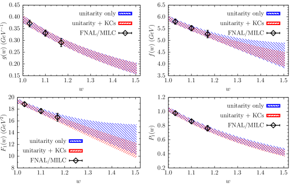
Figure 1: The bands of the FFs $g(w)$, $f(w)$, $\mathcal{F}_{1}(w)$ and $P_{1}(w)$ computed by the DM method after imposing either the unitarity filters only (bue bands) or the unitarity filters and the two KCs (1)-(2) (red bands). The FNAL/MILC values FermilabLattice:2021cdg used as inputs for the DM method are represented by the black diamonds.

III Determination of $\mathbf{|V_{cb}|}$

We start from the measurements of the differential decay widths performed by the Belle Collaboration for the semileptonic $B\to D^{*}\ell\nu_{\ell}$ decays Abdesselam:2017kjf ; Waheed:2018djm . We now determine a new exclusive estimate of $|V_{cb}|$ by performing a bin-per-bin study of the Belle experimental data. The latter ones are given in the form of 10-bins distribution of the quantity $d\Gamma/dx$, where $x$ is one of the four kinematical variables of interest ($x=w,\cos\theta_{l},\cos\theta_{v},\chi$) (see Martinelli:2021onb for the expressions of the four-dimensional differential decay widths and Refs. Abdesselam:2017kjf ; Waheed:2018djm for the specific values of the four variables $x$ in each bin). First of all, we generate a sample of values of the FFs $g$, $f$, $\mathcal{F}_{1}$ and $P_{1}$ to be used for each of the experimental bins using the DM method described in the previous Section. With such FFs we compute the theoretical predictions $d\Gamma^{th}/dx/|V_{cb}|^{2}$ for each experimental bin. We also generate an independent sample of values of the experimental differential decay widths $d\Gamma^{exp}/dx$ for all the bins. For each event of the sample we compute $|V_{cb}|$ as the square root of the ratio of the experimental over the theoretical differential decay widths for all the bins. Using the produced events for $|V_{cb}|$, whose distribution turns out to be very well approximated by a Gaussian Ansatz, we compute the mean values $|V_{cb}|_{i}$ and the corresponding covariance matrix $\mathbf{C}_{ij}$ for all the bins ($i,j=1,...,10$). Finally, adopting the best constant fit over the 10 bins we compute $|V_{cb}|$ and its variance $\sigma^{2}_{|V_{cb}|}$ for each of the four kinematical variables and for each of the two experiments Abdesselam:2017kjf ; Waheed:2018djm as

$$|V_{cb}| = \frac{\sum_{i,j=1}^{10}(\mathbf{C}^{-1})_{ij}|V_{cb}|_{j}}{\sum_{i,j=1}^{10}(\mathbf{C}^{-1})_{ij}}~{},~{}$$ (4)

$$\sigma^{2}_{|V_{cb}|} = \frac{1}{\sum_{i,j=1}^{10}(\mathbf{C}^{-1})_{ij}}~{}.~{}$$ (5)

In Fig. 2 we show the bin-per-bin distributions of $|V_{cb}|$ for each kinematical variable $x$ and for each experiment, together with their final weighted mean values. The latter ones are collected also in Table 1 together with the corresponding values of the reduced $\chi^{2}$-variable, $\chi^{2}/(\mbox{d.o.f.})$, being the number of d.o.f. equal to 9. As already noted in Ref. Martinelli:2021onb , we observe anomalous underestimates of the mean values of $|V_{cb}|$ in the case of some of the variables $x$, which correspond also to large values of the reduced $\chi^{2}$-variable.

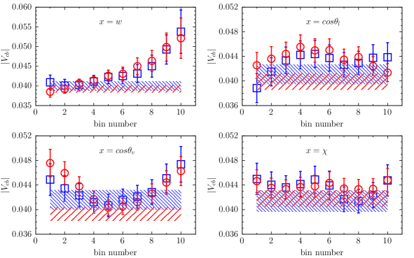
Figure 2: The bin-per-bin estimates of $|V_{cb}|$ and their weighted means (4)-(5) for each kinematical variable $x$ and for each experiment adopting the original covariance matrices of the Belle experiments. The blue squares and the red circles correspond respectively to the first Abdesselam:2017kjf and to the second Waheed:2018djm set of the Belle measurements. The dashed blue (red) bands are the results of Eqs. (4)-(5) in the case of the blue squares (red circles) for each variable $x$ (see Refs. Abdesselam:2017kjf ; Waheed:2018djm for the specific values of the four variables $x$ in each bin).

experiment	$|V_{cb}|(x=w)$	$|V_{cb}|(x=\mbox{cos}\theta_{l})$	$|V_{cb}|(x=\mbox{cos}\theta_{v})$	$|V_{cb}|(x=\chi)$
Ref. Abdesselam:2017kjf	0.0399 (12)	0.0411 (16)	0.0416 (16)	0.0414 (17)
$\chi^{2}/(\mbox{d.o.f.})$	1.72	1.10	1.21	1.45
Ref. Waheed:2018djm	0.0392  (9)	0.0399 (13)	0.0393 (11)	0.0418 (13)
$\chi^{2}/(\mbox{d.o.f.})$	1.62	2.41	3.77	0.79

Table 1: Mean values and uncertainties of the CKM element $|V_{cb}|$ obtained by the correlated average (4)-(5) for each of the four kinematical variables $x$ and for each of the two experiments Abdesselam:2017kjf ; Waheed:2018djm adopting the original covariance matrices of the Belle experiments. The corresponding values of the reduced $\chi^{2}$-variable, $\chi^{2}/(\mbox{d.o.f.})$, are also shown.

We adopt the alternative strategy described in Ref. Martinelli:2021onb for each of the two Belle experiments. We consider the relative differential decay rates given by the ratios $(d\Gamma/dx)/\Gamma$ (where $x=w,\cos\theta_{l},\cos\theta_{v},\chi$) for each bin by using the experimental data. In this way we guarantee that the sum over the bins is exactly independent (event by event) of the choice of the variable $x$. Hence, we compute a new correlation matrix using the events for the ratios $(d\Gamma/dx)/\Gamma$. The new correlation matrix has four eigenvalues equal to zero, because the sum over the bins of each of the four variable $x$ is always equal to unity. In other words, the number of independent bins for the ratios is 36 and not 40 for each experiment. Then, following Ref. Martinelli:2021onb a new covariance matrix of the experimental data is constructed by multiplying the new correlation matrix by the original uncertainties associated to the measurements.

Thus, we repeat the whole procedure for the extraction of $|V_{cb}|$ using the new experimental covariance matrices. In Fig. 3 we show the bin-per-bin distributions of $|V_{cb}|$ for each kinematical variable $x$ and for each experiment, together with their final weighted mean values. The latter ones are collected also in Table 2. A drastic improvement of the values of the reduced $\chi^{2}$-variable is obtained for each of the kinematical variable $x$ and for each of the two Belle experiments.

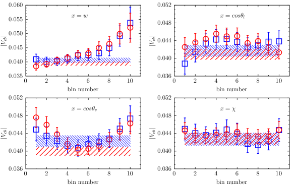
Figure 3: The same as in Fig. 2, but using the new experimental covariance matrices described in the text.

experiment	$|V_{cb}|(x=w)$	$|V_{cb}|(x=\mbox{cos}\theta_{l})$	$|V_{cb}|(x=\mbox{cos}\theta_{v})$	$|V_{cb}|(x=\chi)$
Ref. Abdesselam:2017kjf	0.0405 (9)	0.0417 (13)	0.0422 (13)	0.0427 (14)
$\chi^{2}/(\mbox{d.o.f.})$	1.01	0.89	0.66	0.72
Ref. Waheed:2018djm	0.0394 (7)	0.0409 (12)	0.0400 (10)	0.0427 (13)
$\chi^{2}/(\mbox{d.o.f.})$	1.21	1.36	1.99	0.38

Table 2: The same as in Table 1, but using the new experimental covariance matrices described in the text.

Then, we combine the mean values of Table 2 through the formulæ EuropeanTwistedMass:2014osg

$$\mu_{x} = \frac{1}{N}\sum_{k=1}^{N}x_{k}~{},~{}$$ (6)

$$\sigma_{x}^{2} = \frac{1}{N}\sum_{k=1}^{N}\sigma_{k}^{2}+\frac{1}{N}\sum_{k=1}^{N}(x_{k}-\mu_{x})^{2}~{},~{}$$ (7)

where the second term in the r.h.s. of Eq. (7) accounts for the spread of the values of $|V_{cb}|$ corresponding to the various kinematical variables and experiments. We obtain for each of the two Belle experiments the averages

$$|V_{cb}| = (41.8\pm 1.5)\cdot 10^{-3}\qquad\mbox{Ref.~{}\cite[cite]{\@@bibref{Authors Phrase1YearPhrase2}{Abdesselam:2017kjf}{\@@citephrase{(}}{\@@citephrase{)}}}}~{}$$

$$= (40.8\pm 1.7)\cdot 10^{-3}\qquad\mbox{Ref.~{}\cite[cite]{\@@bibref{Authors Phrase1YearPhrase2}{Waheed:2018djm}{\@@citephrase{(}}{\@@citephrase{)}}}}~{}$$

and by further combining the two Belle experiments the final estimate

$$|V_{cb}|=(41.3\pm 1.7)\cdot 10^{-3}~{},~{}$$ (8)

which is compatible with the most recent inclusive determination $|V_{cb}|_{\rm{incl}}=(42.16\pm 0.50)\cdot 10^{-3}$ Bordone:2021oof at the $0.5\sigma$ level.

Without the modification of the experimental covariance matrices (i.e. using the eight mean values shown in Table 1 and in Fig. 2) the final estimate of $|V_{cb}|$ would have read

$$|V_{cb}|=(40.5\pm 1.7)\cdot 10^{-3}~{},~{}$$

which is still compatible with the most recent inclusive determination at the $1\sigma$ level.

From Fig. 3 we note that:

• in the top left panel the value of $|V_{cb}|$ exhibits some dependence on the specific $w$-bin. The value obtained adopting a constant fit is dominated by the bins at small values of the recoil, where direct lattice data are available and the lenght of the momentum extrapolation is limited;

• in the bottom left panel the value of $|V_{cb}|$ deviates from a constant behavior, as it is also signaled by the large value of the corresponding reduced $\chi^{2}$-variable for the second set of the Belle measurements. Instead of a constant fit, we try a quadratic one of the form $|V_{cb}|\left[1+\delta B\,\mbox{cos}^{2}(\theta_{v})\right]$, suggested by the structure of the differential decay rate $d\Gamma/d\mbox{cos}(\theta_{v})$ within the Standard Model and beyond (see, e.g., Ref. Ivanov:2016qtw )). If the dependence of the experimental and theoretical decay rates upon $\mbox{cos}(\theta_{v})$ were the same, then the parameter $\delta B$ would identically vanish. Instead we get a non-vanishing value of the parameter $\delta B$, namely: $|V_{cb}|=(41.1\pm 1.4)\cdot 10^{-3}$ and $\delta B=0.144\pm 0.074$ for the first set Abdesselam:2017kjf of the Belle measurements, and $|V_{cb}|=(40.8\pm 1.0)\cdot 10^{-3}$ and $\delta B=0.184\pm 0.050$ for the second set Waheed:2018djm . The values of $|V_{cb}|$ are consistent with each other and also with the corresponding values obtained adopting a constant fit and shown in the fourth column of Table 2.

Both observations may be related to a different $w$-slope of the theoretical FFs based on the lattice results of Ref. FermilabLattice:2021cdg with respect to the Belle experimental data Abdesselam:2017kjf ; Waheed:2018djm , as shown in Fig. 4. This crucial issue (a kind of a new slope puzzle) needs to be further investigated by forthcoming calculations of the FFs at non-zero recoil expected from the JLQCD Collaboration Kaneko:2021tlw as well as by future improvements of the precision of the experimental data.

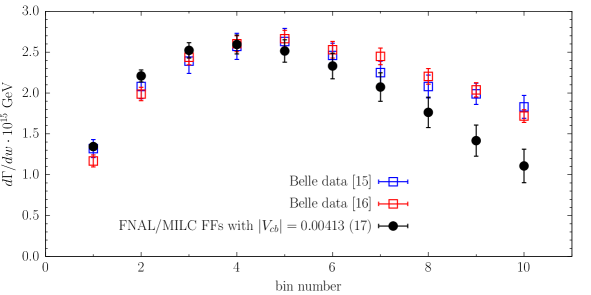
Figure 4: The differential decay width $d\Gamma/dw$ measured by the two Belle experiments Abdesselam:2017kjf ; Waheed:2018djm in the 10 experimental $w$-bins compared with the corresponding theoretical predictions obtained in this work using the DM bands for the FFs, based on the FNAL/MILC synthetic data FermilabLattice:2021cdg (see Fig. 1), and adopting for $|V_{cb}|$ our final determination given by Eq. (8).

IV Evaluation of $R(D^{*})$ and polarization observables

By using the unitarity bands of the FFs we can compute the pure theoretical expectation values of the ratio $R(D^{*})$, the $\tau$-polarization $P_{\tau}(D^{*})$ and the longitudinal $D^{*}$-polarization $F_{L}(D^{*})$, obtaining

$$R(D^{*}) = 0.275\pm 0.008~{},~{}$$

$$P_{\tau}(D^{*}) = -0.529\pm 0.007~{},~{}$$ (9)

$$F_{L}(D^{*}) = 0.414\pm 0.012~{}$$

to be compared with the experimental values

$$R(D^{*})|_{\rm{exp}} = 0.295\pm 0.011\pm 0.008~{}\qquad~{}\mbox{Ref.~{}\cite[cite]{\@@bibref{Authors Phrase1YearPhrase2}{HFLAV:2019otj}{\@@citephrase{(}}{\@@citephrase{)}}}}~{},~{}$$

$$P_{\tau}(D^{*})|_{\exp} = -0.38\pm 0.51^{+0.21}_{-0.16}~{}\qquad\qquad\mbox{Ref.~{}\cite[cite]{\@@bibref{Authors Phrase1YearPhrase2}{Belle:2016dyj}{\@@citephrase{(}}{\@@citephrase{)}}}}~{},~{}$$ (10)

$$F_{L}(D^{*})|_{\exp} = 0.60\pm 0.08\pm 0.04~{}\qquad\qquad\mbox{Ref.~{}\cite[cite]{\@@bibref{Authors Phrase1YearPhrase2}{Belle:2019ewo}{\@@citephrase{(}}{\@@citephrase{)}}}}~{}.~{}$$

While the theoretical and the experimental values of $P_{\tau}(D^{*})$ are in agreement (mainly due to the larger experimental uncertainty), the compatibility for $R(D^{*})$ and $F_{L}(D^{*})$ is at the $\sim 1.3\sigma$ and $\sim 2.1\sigma$ level, respectively. Note that the $R(D^{*})$ anomaly results to be smaller with respect to the $\sim 2.5\sigma$ tension stated by HFLAV Collaboration HFLAV:2019otj .

In Ref. Martinelli:2021onb the DM method was applied to the final lattice data for the $B\to D\ell\nu_{\ell}$ transition provided by the FNAL/MILC Collaboration MILC:2015uhg . We obtained for the ratio $R(D)$ the pure theoretical estimate $R(D)=0.296\pm 0.008$, which is consistent with the experimental world average $R(D)|_{\rm{exp}}=0.340\pm 0.027\pm 0.013$ HFLAV:2019otj at the $\sim 1.4\sigma$ level. In Fig. 5 we show the comparison of the DM results for the two ratios $R(D)$ and $R(D^{*})$ with the corresponding experimental world averages from HFLAV HFLAV:2019otj .

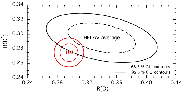
Figure 5: The contour plots of the DM results for the ratios $R(D)$ and $R(D^{*})$, obtained respectively in Ref. Martinelli:2021onb and in this work, compared with those corresponding to the experimental world averages from HFLAV HFLAV:2019otj .

Note that we have considered our values for $R(D)$ and $R(D^{*})$ as uncorrelated. This is motivated by the absence of any information about possible correlations among the lattice FFs entering the $B\to D$ and $B\to D^{*}$ decays and by the fact that the correlation induced by the vector transverse susceptibility $\chi_{1^{-}}(0)$, which is present in both channels, is very mild, as we have explicitly checked.

V Conclusions

In this work we have applied the DM method DiCarlo:2021dzg ; Martinelli:2021onb to the lattice computations of the FFs entering the semileptonic $B\to D^{*}\ell\nu_{\ell}$ decays, produced recently by the FNAL/MILC Collaborations FermilabLattice:2021cdg at small, non-zero values of the recoil. Thanks to the DM method the FFs have been extrapolated in the whole kinematical range accessible to the semileptonic decays in a completely model-independent and non-perturbative way, implementing exactly both unitarity and kinematical constraints.

Using our theoretical bands of the FFs we have determined $|V_{cb}|$ from the experimental data and computed $R(D^{*})$ from theory. Our final result for $|V_{cb}|$ is $|V_{cb}|=(41.3\pm 1.7)\cdot 10^{-3}$, which is compatible with the latest inclusive determination $|V_{cb}|_{\rm{incl}}=(42.16\pm 0.50)\cdot 10^{-3}$ Bordone:2021oof at the $0.5\sigma$ level. Moreover, we have obtained the pure theoretical value $R(D^{*})=0.275\pm 0.008$, which is compatible with the experimental world average at the $\sim 1.3\sigma$ level. Together with future improvements of the precision of experimental data, new forthcoming lattice determinations of the FFs at non-zero recoil, expected from the JLQCD Collaboration Kaneko:2021tlw , will be crucial to confirm our present indication of a sizable reduction of the $|V_{cb}|$ puzzle.

Appendix A The DM method

In this Appendix we briefly recall the main features of the DM method applied to the description of a generic FF $f(q^{2})$ with definite spin-parity.

Let us consider a set of $N$ values of the FF, $\{f\}=\{f(z_{j})\}$ with $j=1,2,...,N$, where $z$ is the conformal variable

$$z(q^{2})\equiv\frac{\sqrt{t_{+}-q^{2}}-\sqrt{t_{+}-t_{-}}}{\sqrt{t_{+}-q^{2}}+\sqrt{t_{+}-t_{-}}}~{}$$ (11)

with $t_{\pm}\equiv(m_{B}\pm m_{D^{*}})^{2}$ in the case of our interest and $z_{j}\equiv z(q_{j}^{2})$. Then, the FF at a generic value of $z=z(q^{2})$ is bounded by unitarity, analyticity and crossing symmetry to be in the range DiCarlo:2021dzg

$$\beta(z)-\sqrt{\gamma(z)}\leq f(z)\leq\beta(z)+\sqrt{\gamma(z)}~{},~{}$$ (12)

where

$$\beta(z) \equiv \frac{1}{\phi(z,q_{0}^{2})d(z)}\sum_{j=1}^{N}f(z_{j})\phi(z_{j},q_{0}^{2})d_{j}\frac{1-z_{j}^{2}}{z-z_{j}}~{},~{}$$ (13)

$$\gamma(z) \equiv \frac{1}{1-z^{2}}\frac{1}{\phi^{2}(z,q_{0}^{2})d^{2}(z)}\left[\chi(q_{0}^{2})-\chi_{\{f\}}^{DM}(q_{0}^{2})\right]~{},~{}$$ (14)

$$\chi_{\{f\}}^{DM}(q_{0}^{2}) \equiv \sum_{i,j=1}^{N}f(z_{i})f(z_{j})\phi(z_{i},q_{0}^{2})\phi(z_{j},q_{0}^{2})d_{i}d_{j}\frac{(1-z_{i}^{2})(1-z_{j}^{2})}{1-z_{i}z_{j}}~{}$$ (15)

with

$$d(z)\equiv\prod_{m=1}^{N}\frac{1-zz_{m}}{z-z_{m}}~{},~{}\qquad d_{j}\equiv\prod_{m\neq j=1}^{N}\frac{1-z_{j}z_{m}}{z_{j}-z_{m}}~{}.~{}$$ (16)

In the above Equations $\chi(q_{0}^{2})$ is the dispersive bound, evaluated at an auxiliary value $q_{0}^{2}$ of the squared 4-momentum transfer using suitable two-point correlators, and $\phi(z,q_{0}^{2})$ is a kinematical function appropriate for the given form factor Boyd:1997kz . The kinematical function $\phi$ may contain the contribution of the resonances below the pair production threshold $t_{+}$.

Unitarity is satisfied only when $\gamma(z)\geq 0$, which implies

$$\chi(q_{0}^{2})\geq\chi_{\{f\}}^{DM}(q_{0}^{2})~{}.~{}$$ (17)

Since $\chi_{\{f\}}^{DM}(q_{0}^{2})$ does not depend on $z$, Eq. (17) is either never verified or always verified for any value of $z$. This leads to the first important feature of our method: the DM unitarity filter (17) represents a parameterization-independent implementation of unitarity for the given set of input values $\{f\}$ of the FF.

We point out another important feature of the DM approach. When $z$ coincides with one of the data points, i.e. $z\to z_{j}$, one has $\beta(z)\to f(z_{j})$ and $\gamma(z)\to 0$. In other words the DM method reproduces exactly the given set of data points. This leads to the second important feature of our method: the DM band given in Eq. (12) is equivalent to the results of all possible fits that satisfy unitarity and at the same time reproduce exactly the input data.

The above features may not be shared by truncated parameterisations based on the $z$-expansion, like the Boyd-Grinstein-Lebed (BGL) Boyd:1997kz fits. Indeed, there is no guarantee that truncated BGL parameterizations reproduce exactly the set of input data and, consequently, the fulfillment of the unitarity constraint may fictitiously depend upon the order of the truncation.

Appendix B The unitarity filters

The non-perturbative values of the dispersive bounds corresponding to the $b\to c$ transition for channels with definite spin-parity have been computed on the lattice at $q_{0}^{2}=0$ in Ref. Martinelli:2021frl . After subtraction of the contribution of bound states the susceptibilities relevant for the $B\to D^{*}\ell\nu_{\ell}$ decays are given by

$$\chi_{1^{-}}(0) = (5.84\pm 0.44)\cdot 10^{-4}~{}\mbox{GeV}^{-2}~{},~{}$$ (18)

$$\chi_{0^{-}}(0) = (21.9\pm 1.9)\cdot 10^{-3}~{},~{}$$

$$\chi_{1^{+}}(0) = (4.69\pm 0.30)\cdot 10^{-4}~{}\mbox{GeV}^{-2}~{},~{}$$

The kinematical functions associated to the semileptonic FFs reads Boyd:1997kz

$$\phi_{g}(z) = 16r^{2}\sqrt{\frac{2}{3\pi}}\frac{(1+z)^{2}}{\sqrt{1-z}\left[(1+r)(1-z)+2\sqrt{r}(1+z)\right]^{4}}~{},~{}$$

$$\phi_{f}(z,0) = 4\frac{r}{m_{B}^{2}}\sqrt{\frac{2}{3\pi}}\,\frac{(1+z)(1-z)^{3/2}}{\left[(1+r)(1-z)+2\sqrt{r}(1+z)\right]^{4}}~{},~{}$$

$$\phi_{\mathcal{F}_{1}}(z,0) = 4\frac{r}{m_{B}^{3}}\sqrt{\frac{1}{3\pi}}\frac{(1+z)(1-z)^{5/2}}{\left[(1+r)(1-z)+2\sqrt{r}(1+z)\right]^{5}}~{},~{}$$ (19)

$$\phi_{P_{1}}(z,0) = 16\,(1+r)r^{3/2}\sqrt{\frac{1}{\pi}}\frac{(1+z)^{2}}{\sqrt{1-z}\left[(1+r)(1-z)+2\sqrt{r}(1+z)\right]^{4}}~{}$$

with $r\equiv m_{D^{*}}/m_{B}$.

The presence of resonances below the pair production threshold lead to the following modification of the kinematical function $\phi(z,0)$ Lellouch:1995yv

$$\phi(z,0)\to\phi(z,0)\cdot\prod_{R}\frac{z-z(m_{R}^{2})}{1-z\,z(m_{R}^{2})}~{},~{}$$ (20)

where $m_{R}$ is the mass of the resonance $R$. For the masses of the poles corresponding to $B_{c}^{(*)}$ mesons with different quantum numbers entering the various FFs we refer to Table III of Ref. Bigi:2017jbd . We note that in the case of the $B\to D^{*}$ decay the conformal variable $z$ (see Eq. (11)) ranges from $z(q^{2}=t_{-})=0$ to $z(q^{2}=0)=0.056$ and $z(m_{R}^{2})<0$. Thus, the accurate location of the poles in Eq. (20) is not crucial.

According to Ref.  Boyd:1997kz there are three unitarity constraints on the FFs of the $B\to D^{*}\ell\nu_{\ell}$ decays, namely

$$\chi_{1^{-}}(0) \geq \chi_{\{g\}}^{DM}(0)~{},~{}$$ (21)

$$\chi_{1^{+}}(0) \geq \chi_{\{f\}}^{DM}(0)+\chi_{\{\mathcal{F}_{1}\}}^{DM}(0)~{},~{}$$ (22)

$$\chi_{0^{-}}(0) \geq \chi_{\{P_{1}\}}^{DM}(0)~{},~{}$$ (23)

where $\chi_{\{g,f,\mathcal{F}_{1},P_{1}\}}^{DM}(0)$ are given by Eq. (17) in terms of the known values of the corresponding FF.

Appendix C Implementation of the kinematical constraints

In this Appendix we summarize the basic steps of the procedure adopted to fulfill the KCs (1)-(2) in our sample of events for the FFs. For ease of presentation we limit ourselves to the KC (1) at minimum recoil $w=1$, which can be rewritten as

$$\mathcal{F}_{1}(1)=\widetilde{f}(1)~{},~{}$$ (24)

where the FF $\widetilde{f}(w)$ is defined simply as $\widetilde{f}(w)=m_{B}(1-r)f(w)$.

We start from a sample of events, each of which is composed by 15 numbers: 12 values of the synthetic lattice points of the FFs (four FFs at three values of the recoil $w$) and the 3 values of the susceptibilities $\chi_{1^{-}}(0)$, $\chi_{0^{-}}(0)$ and $\chi_{1^{+}}(0)$. The sample is generated using a covariance matrix of input data with dimension $15\times 15$. We consider that the unitarity filters (21)-(23) have been already applied, as described in Section II, so that the sample is composed by events all passing the unitarity filters.

For each event we evaluate Eq. (12) for the two FFs $\mathcal{F}_{1}$ and $f$ at $w=1$ (corresponding to $z=0$), obtaining in this way two lower and two upper bounds, namely $\mathcal{F}_{1}^{lo(up)}(1)$ and $\widetilde{f}^{lo(up)}(1)$. Then, we consider only the events for which the dispersive bands for the two FFs overlap each other and for these events we evaluate the intersection between the above bounds to obtain the lower and upper bounds for the common value $\overline{f}(1)$ of the KC (24) , viz.

$$\overline{f}^{lo}(1) = \mbox{max}\left[\mathcal{F}_{1}^{lo}(1),~{}\widetilde{f}^{lo}(1)\right]~{},~{}$$

$$\overline{f}^{up}(1) = \mbox{min}\left[\mathcal{F}_{1}^{up}(1),~{}\widetilde{f}^{up}(1)\right]~{},~{}$$

so that

$$\overline{f}^{lo}(1)\leq\overline{f}(1)\leq\overline{f}^{up}(1)~{},~{}$$ (25)

where $\overline{f}(1)\equiv\mathcal{F}_{1}(1)=\widetilde{f}(1)$. As discussed in Ref. DiCarlo:2021dzg , we consider the value $\overline{f}(1)$ to be uniformly distributed in the range given by Eq. (25).

We repeat the above steps for all the events of the FFs and, using the subset of events for which the dispersive bands for the two FFs overlap each other, we evaluate the mean values $<\overline{f}^{lo(up)}(1)>$, the standard deviations $\sigma^{lo(up)}$ and the correlations with all the other input data and the one among the bounds, i.e. $\rho^{lo,up}$. It follows (see Section V-C of Ref. DiCarlo:2021dzg ) that the mean value and the variance for the FF $\overline{f}(1)$ are given by

$$<\overline{f}(1)> = \frac{1}{2}\left[<\overline{f}^{lo}(1)>+<\overline{f}^{up}(1)>\right]~{},~{}$$ (26)

$$\sigma_{\overline{f}(1)}^{2} = \frac{1}{12}\left[<\overline{f}^{up}(1)>-<\overline{f}^{lo}(1)>\right]^{2}+\frac{1}{3}\left[(\sigma^{lo})^{2}+(\sigma^{up})^{2}+\rho^{lo,up}\,\sigma^{lo}\,\sigma^{up}\right]~{}.~{}$$ (27)

Therefore, we increase by one the dimension of the events of our sample by adding the FF $\overline{f}(1)$ at $w=1$ normally distributed with mean value (26) and variance (27). Analogously, the dimension of the covariance matrix of the input data becomes $16\times 16$. The added point is used for evaluating both $\mathcal{F}_{1}(w)$ and $f(w)$ at a generic value of the recoil $w$.

We repeat the above procedure also for the KC (2) at maximum recoil.

References

- (1) M. Di Carlo, G. Martinelli, M. Naviglio, F. Sanfilippo, S. Simula and L. Vittorio, Unitarity bounds for semileptonic decays in lattice QCD, Phys. Rev. D 104 (2021) 054502 [2105.02497].
- (2) G. Martinelli, S. Simula and L. Vittorio, and ) using lattice QCD and unitarity, Phys. Rev. D 105 (2022) 034503 [2105.08674].
- (3) Fermilab Lattice, MILC collaboration, Semileptonic form factors for at nonzero recoil from 2 + 1-flavor lattice QCD, 2105.14019.
- (4) L. Lellouch, Lattice constrained unitarity bounds for anti-B0 — pi+ lepton- anti-lepton-neutrino decays, Nucl. Phys. B 479 (1996) 353 [hep-ph/9509358].
- (5) G. Martinelli, S. Simula and L. Vittorio, Constraints for the semileptonic B→D(*) form factors from lattice QCD simulations of two-point correlation functions, Phys. Rev. D 104 (2021) 094512 [2105.07851].
- (6) M. Bordone, B. Capdevila and P. Gambino, Three loop calculations and inclusive Vcb, Phys. Lett. B 822 (2021) 136679 [2107.00604].
- (7) C. Alpigiani et al., Unitarity Triangle Analysis in the Standard Model and Beyond, in 5th Large Hadron Collider Physics Conference, 10, 2017 [1710.09644].
- (8) A.J. Buras and E. Venturini, Searching for New Physics in Rare and Decays without and Uncertainties, 2109.11032.
- (9) D. Bigi and P. Gambino, Revisiting , Phys. Rev. D 94 (2016) 094008 [1606.08030].
- (10) S. Jaiswal, S. Nandi and S.K. Patra, Extraction of from and the Standard Model predictions of , JHEP 12 (2017) 060 [1707.09977].
- (11) Flavour Lattice Averaging Group collaboration, FLAG Review 2019: Flavour Lattice Averaging Group (FLAG), Eur. Phys. J. C 80 (2020) 113 [1902.08191].
- (12) HFLAV collaboration, Averages of b-hadron, c-hadron, and -lepton properties as of 2018, Eur. Phys. J. C 81 (2021) 226 [1909.12524].
- (13) G. D’Agostini, Skeptical combination of experimental results using JAGS/rjags with application to the K± mass determination, 2001.03466.
- (14) G. D’Agostini, On a curious bias arising when the scaling prescription is first applied to a sub-sample of the individual results, 2001.07562.
- (15) Belle collaboration, Precise determination of the CKM matrix element with decays with hadronic tagging at Belle, 1702.01521.
- (16) Belle collaboration, Measurement of the CKM matrix element from at Belle, Phys. Rev. D 100 (2019) 052007 [1809.03290].
- (17) BaBar collaboration, Extraction of form Factors from a Four-Dimensional Angular Analysis of , Phys. Rev. Lett. 123 (2019) 091801 [1903.10002].
- (18) European Twisted Mass collaboration, Up, down, strange and charm quark masses with Nf = 2+1+1 twisted mass lattice QCD, Nucl. Phys. B 887 (2014) 19 [1403.4504].
- (19) M.A. Ivanov, J.G. Körner and C.-T. Tran, Analyzing new physics in the decays with form factors obtained from the covariant quark model, Phys. Rev. D 94 (2016) 094028 [1607.02932].
- (20) T. Kaneko, Y. Aoki, B. Colquhoun, M. Faur, H. Fukaya, S. Hashimoto et al., semileptonic decays in lattice QCD with domain-wall heavy quarks, in 38th International Symposium on Lattice Field Theory, 12, 2021 [2112.13775].
- (21) Belle collaboration, Measurement of the lepton polarization and in the decay , Phys. Rev. Lett. 118 (2017) 211801 [1612.00529].
- (22) Belle collaboration, Measurement of the polarization in the decay , in 10th International Workshop on the CKM Unitarity Triangle, 3, 2019 [1903.03102].
- (23) MILC collaboration, B→D form factors at nonzero recoil and —Vcb— from 2+1-flavor lattice QCD, Phys. Rev. D 92 (2015) 034506 [1503.07237].
- (24) C. Boyd, B. Grinstein and R.F. Lebed, Precision corrections to dispersive bounds on form-factors, Phys. Rev. D 56 (1997) 6895 [hep-ph/9705252].
- (25) D. Bigi, P. Gambino and S. Schacht, , , and the Heavy Quark Symmetry relations between form factors, JHEP 11 (2017) 061 [1707.09509].