Parton physics from a heavy-quark operator product expansion:
Lattice QCD calculation of the second moment
of the pion distribution amplitude

Abstract

The pion light-cone distribution amplitude (LCDA) is a central non-perturbative object of interest for high-energy exclusive processes in quantum chromodynamics. In this article, the second Mellin moment of the pion LCDA is determined as a proof-of-concept calculation for the first numerical implementation of the heavy-quark operator product expansion (HOPE) method. The resulting value for the second Mellin moment, determined in quenched QCD at a pion mass of $m_{\pi}=550$ MeV at a factorization scale of 2 GeV is $\expectationvalue{\xi^{2}}=0.210\pm 0.013\text{ (stat.)}\pm 0.034\text{ (sys.)}$. This result is compatible with those from previous determinations of this quantity.

HOPE Collaboration

I Introduction

The pion light-cone distribution amplitude (LCDA) plays an important role in parton physics. It is central to a description of a range of exclusive processes in high energy quantum chromodynamics Lepage and Brodsky (1980). This LCDA, denoted as $\phi_{\pi}$, is defined via its relation to the matrix element for the transition between the vacuum and the (charged) pion state,

$$\langle 0|\overline{\psi}_{d}(z)\gamma_{\mu}\gamma_{5}W[z,-z]\psi_{u}(-z)|\pi^{+}({\mathbf{p}})\rangle=ip_{\mu}f_{\pi}\int_{-1}^{1}d\xi\mbox{ }{\mathrm{e}}^{-i\xi p\cdot z}\phi_{\pi}(\xi,\mu)\,,$$ (1)

where $\mu$ is the renormalization scale and ${\mathcal{W}}[-z,z]$ is a light-like Wilson line between light-cone coordinates $-z$ to $z$ ($z^{2}=0$). In the above equation, $f_{\pi}$, ${\mathbf{p}}$, and $p_{\mu}$ are the decay constant, the three-momentum, and the four-momentum of the pion. In the light-cone gauge, $\phi_{\pi}(\xi,\mu)$ can be interpreted as the probability amplitude for the pion to transition to the state of a quark and an antiquark that carry $(1+\xi)/2$ and $(1-\xi)/2$ fractions of the pion momentum, respectively Lepage and Brodsky (1980). This LCDA plays an important role in understanding exclusive processes in QCD Radyushkin (1977); Lepage and Brodsky (1980), in addition to being a crucial ingredient for extracting information regarding the Cabibbo-Kobayashi-Maskawa matrix in flavour physics via hadronic decays of the $B$ meson Dugan and Grinstein (1991); Beneke et al. (1999); Keum et al. (2001); Bauer et al. (2006).

Since $\phi_{\pi}(\xi,\mu)$ encodes non-perturbative physics from strong interactions, it is natural to attempt to compute this quantity with lattice QCD (LQCD). However, LQCD calculations are normally carried out in Euclidean space because of the need to employ Monte-Carlo methods in evaluating the path integrals. Therefore it is challenging to adopt LQCD for investigating parton physics which involves dynamics on the light cone. This leads to the conventional LQCD approach of determining the Mellin moments for various parton distribution functions (PDFs) and LCDAs. In general these moments can be extracted by computing matrix elements of local operators that result from an operator product expansion (OPE) Kronfeld and Photiadis (1985); Martinelli and Sachrajda (1987); Del Debbio et al. (2003); Arthur et al. (2011); Bali et al. (2019a). The analytic continuation between Euclidean and Minkowski spaces for these matrix elements is straightforward. In principle, knowledge of the relevant Mellin moments enables the construction of PDFs and LCDAs. Nevertheless, such a strategy has been limited by the possibility of having reliable LQCD results for only the first few moments because the breaking of $O(4)$ Euclidean space-time symmetry by the lattice regularization requires the subtraction of power divergences in the renormalization of the relevant local operators Kronfeld and Photiadis (1985). These power divergences already appear in the computation of the first non-trivial (the second) Mellin moment for $\phi_{\pi}(\xi,\mu)$. They can be evaded by using a method proposed in Ref. Martinelli and Sachrajda (1987), where one chooses particular combinations of the Lorentz indices in the local operator for computing the second moment. However, this method is not applicable for the extraction of higher moments, making it desirable to have other approaches with which to extract information of LCDAs and other light-cone quantities, including PDFs.

Alternative strategies for extracting information about LCDAs and PDFs using LQCD have been proposed in the last two decades Aglietti et al. (1998); Liu (2000); Detmold and Lin (2006); Braun and Müller (2008); Davoudi and Savage (2012); Ji (2013); Chambers et al. (2017); Radyushkin (2017); Ma and Qiu (2018), and their implementations are being intensively pursued, see Refs. Cichy and Constantinou (2019); Ji et al. (2020); Constantinou (2021); Constantinou et al. (2020) for reviews. To access information contained in higher Mellin moments while bypassing the above-mentioned complication in renormalizing the local operators, a generic character of these strategies is the computation for hadronic matrix elements of non-local operators. For instance, one much studied procedure, the quasi-PDF approach Ji (2013), features the calculation of matrix elements involving a space-like Wilson line. This work follows the method suggested in Ref. Detmold and Lin (2006). It relies on investigating the OPE analysis for hadronic amplitudes in Euclidean space with the insertion of two local quark bilinears that contain a fictitious, valence heavy quark. For this reason, this approach is termed the heavy-quark OPE (HOPE) method. The introduction of this heavy quark affords several advantages, such the removal of certain higher-twist effects, the inclusion of an extra heavy scale to control the OPE, and simple properties of analytic continuation to Minkowski space. As pointed out in recent work Detmold et al. (2021), this method can be used to extract the $\xi$-dependence in $\phi_{\pi}(\xi,\mu)$ through a perturbative matching procedure. The current article presents its application to the numerical determination of the (second) Mellin and Gegenbauer moments. Since this is the first numerical implementation of the HOPE strategy, this calculation bears the character of a feasibility study, which investigates the relatively well-known second Mellin moment. This allows a better quantification of the efficacy of the method. The success of the current work paves the way for further studies using this technique. For this reason, the quenched approximation and an unphysical pion mass of $\sim 550$ MeV are used. Since the continuum extrapolation is an important ingredient in this approach, the calculations are performed at four choices of the lattice spacing, $a$, ranging from 0.04 fm to 0.08 fm.

Definitions relevant to this method and the conventions adopted in this article are declared in Sec. II. The HOPE method and its particular features for the current work are explained in Sec. III, while Sec. IV describes the details of the numerical implementation. The analysis of the data and the results are discussed in Sec. V. The conclusion of this work and the outlook in this research direction are then given in Sec. VI.

II Definitions and conventions

Before proceeding to describe the numerical lattice determination for the second Mellin and Gegenbauer moments of $\phi_{\pi}(\xi,\mu)$, a review of the definition of these moments is in order. The discussion presented here also serves the purpose of setting the conventions and notation that will be used in subsequent calculations.

Conformal symmetry in QCD Braun et al. (2003) implies that the pion LCDA can be conveniently studied using the Gegenbauer OPE. $C$-parity imposes the constraint $\phi_{\pi}(\xi,\mu)=\phi_{\pi}(-\xi,\mu)$ in the isospin limit, leading to

$$\phi_{\pi}(\xi,\mu)=\frac{3}{4}(1-\xi^{2})\sum_{n=0,{\mathrm{even}}}^{\infty}\phi_{n}(\mu){\mathcal{C}}_{n}^{3/2}(\xi)\,,$$ (2)

where ${\mathcal{C}}_{n}^{3/2}(\xi)$ are the Gegenbauer polynomials, with $\mathcal{C}_{0}^{3/2}(\xi)=1$ and $\mathcal{C}_{2}^{3/2}(\xi)=(-3+15\xi^{2})/2$. The Gegenbauer moments, $\phi_{n}(\mu)$, are defined as

$$\phi_{n}(\mu)=\frac{2(2n+3)}{3(n+1)(n+2)}\int_{-1}^{1}d\xi\mbox{ }{\mathcal{C}}_{n}^{3/2}(\xi)\phi_{\pi}(\xi,\mu)\,.$$ (3)

Because of conformal symmetry, the $\phi_{n}(\mu)$ do not mix under the renormalization group (RG) evolution at one loop. To this order, their renormalization scale dependence is Efremov and Radyushkin (1980a)

$$\phi_{n}(\mu_{2})=\phi_{n}(\mu_{1})\left(\frac{\alpha_{s}(\mu_{2})}{\alpha_{s}(\mu_{1})}\right)^{\gamma_{n}/\beta_{0}}\,,$$ (4)

where $\alpha_{s}$ is the strong coupling, $\beta_{0}=11-2N_{f}/3$ ($N_{f}$ being the number of flavours) is the coefficient of the leading-order (LO) QCD $\beta$-function, and $\gamma_{n}$ is the anomalous dimension,

$$\gamma_{n}=\frac{4}{3}\left[1-\frac{2}{(n+1)(n+2)}+4\sum_{j=2}^{n+1}j^{-1}\right]\,.$$ (5)

Since $\gamma_{n}$ increases monotonically with $n$, one expects that a truncated version of the OPE in Eq. (2) can be a good approximation to $\phi_{\pi}(\xi,\mu)$ at large enough renormalization scales. In the regime where $\mu\gg\Lambda_{{\mathrm{QCD}}}$ (with $\Lambda_{{\mathrm{QCD}}}$ being the QCD dynamical scale), the pion LCDA is dominated by the zeroth Gegenbauer moment. Equations (4) and (5) lead to the asymptotic form the pion LCDA,

$$\lim_{\mu\rightarrow\infty}\phi_{\pi}(\xi,\mu)=\frac{3}{4}\left(1-\xi^{2}\right)\,,$$ (6)

where the normalization $\phi_{0}=1$ has been imposed.

The Gegenbauer moments in Eqs. (2) and (3) can be expressed as linear combinations of the Mellin moments $\langle\xi^{n}\rangle$, which are defined as

$$\langle\xi^{n}\rangle(\mu)=\int_{-1}^{1}d\xi\mbox{ }\xi^{n}\phi_{\pi}(\xi,\mu)\,.$$ (7)

For instance, from Eqs. (2) and (7) it is straightforward to obtain

$$\phi_{0}=\langle\xi^{0}\rangle=1\,,\,\,\phi_{2}=\frac{7}{12}\left(5\langle\xi^{2}\rangle-\langle\xi^{0}\rangle\right)\,,\,\,\phi_{4}=\frac{11}{24}\left(21\langle\xi^{4}\rangle-14\langle\xi^{2}\rangle+\langle\xi^{0}\rangle\right)\,,\ldots\,.$$ (8)

In general, knowledge of $\langle\xi^{0}\rangle$, $\langle\xi^{2}\rangle$, …, $\langle\xi^{n}\rangle$ is equivalent to that of $\phi_{0}$, $\phi_{2}$, …, $\phi_{n}$. These Mellin moments, $\langle\xi^{n}\rangle$, can be related to matrix elements of local, twist-two, operators,

$$\langle 0|\big{[}\overline{d}\gamma^{\{\mu_{0}}\gamma_{5}(i\overset{\leftrightarrow}{D}\vphantom{D}^{\,\mu_{1}})\dots(i\overset{\leftrightarrow}{D}\vphantom{D}^{\,\mu_{n}\}})u-{\mathrm{traces}}\big{]}|\pi^{+}(\mathbf{p})\rangle=f_{\pi}\expectationvalue{\xi^{n}}(\mu^{2})\left[p^{\mu_{0}}p^{\mu_{1}}\dots p^{\mu_{n}}-{\mathrm{traces}}\right]\,,$$ (9)

where the Lorentz indices are totally symmetrized, with

$$\overset{\leftrightarrow}{D}\vphantom{D}^{\,\mu}=\frac{1}{2}(\overset{\rightarrow}{D}\vphantom{D}^{\,\mu}-\overset{\leftarrow}{D}\vphantom{D}^{\,\mu})\,,$$ (10)

and the traces are taken in all possible pairs amongst the Lorentz indices, $\mu_{0},\mu_{1},\ldots,\mu_{n}$. As discussed in the last paragraph, from the leading-order result of QCD perturbation theory, it is natural to expect that knowledge of the first few Gegenbauer moments allows one to construct $\phi_{\pi}(\xi,\mu)$ reliably at sufficiently large $\mu$. This also implies that obtaining important information about the LCDA at $\mu\gg\Lambda_{{\mathrm{QCD}}}$ is possible from the first few Mellin moments. This point can be illustrated by investigating an extreme scenario where one truncates the Gegenbauer OPE in Eq. (2) at $n=2$. The pion LCDA constructed with this truncated OPE is denoted $\phi_{\pi}^{(2)}(\xi,\mu)$. Using Eq. (8), one obtains

$$\phi_{\pi}^{(2)}(\xi,\mu) = \frac{3}{4}(1-\xi^{2})\left[\phi_{0}(\mu){\mathcal{C}}^{3/2}_{0}(\xi)+\phi_{2}(\mu){\mathcal{C}}^{3/2}_{2}(\xi)\right]$$ (11)

$$= \frac{15}{32}\left[3-7\langle\xi^{2}\rangle(\mu)\right]+\frac{16}{15}\left[-5+21\langle\xi^{2}\rangle(\mu)\right]\xi^{2}+\frac{105}{32}\left[1-5\langle\xi^{2}\rangle(\mu)\right]\xi^{4}\,.$$

Figure 1 shows the result with $\phi_{\pi}^{(2)}(\xi,\mu)$ at $\langle\xi^{2}\rangle(\mu)=0.2$, 0.25 and 0.3.

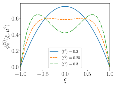
Figure 1: Dependence of $\phi_{\pi}^{(2)}(\xi,\mu)$, defined in Eq. (11), on the values of $\langle\xi^{2}\rangle$. The range of $\langle\xi^{2}\rangle$ values shown in the plot covers typical results for this second Mellin moment at $\mu\sim 2$ GeV from modern lattice computations. They lead to consistency with a single-humped or double-humped structure of the DA, and more precise measurements would resolve this.

Note that these are typical values for this second Mellin moment at $\mu\sim 2$ GeV from modern lattice computations Del Debbio et al. (2003); Arthur et al. (2011); Bali et al. (2018a); Zhang et al. (2017); Bali et al. (2019a). This figure demonstrates that the shape of the pion LCDA can depend strongly upon $\langle\xi^{2}\rangle(\mu)$. Naturally, the inclusion of higher moments will likely reduce the sensitivity to the second moment, but nevertheless, this exercise shows that the second Mellin moment is a phenomenologically interesting quantity.

III Strategy and correlation functions

To present the calculation for the second Mellin and Gegenbauer moments of $\phi_{\pi}(\xi,\mu)$, it is first necessary to describe the strategy and the correlators that have to be computed using LQCD. To extract moments for the pion LCDA employing the HOPE method, the hadronic amplitudes

$$V^{[\mu\nu]}(q,p)\equiv\frac{V^{\mu\nu}(q,p)-V^{\nu\mu}(q,p)}{2}\,,$$ (12)

are computed, where

$$V^{\mu\nu}(q,p)=\int d^{4}z\mbox{ }{\mathrm{e}}^{iq\cdot z}\mbox{ }\langle 0|{\mathcal{T}}\{J_{A}^{\mu}(z/2)J_{A}^{\nu}(-z/2)\}|\pi({\mathbf{p}})\rangle\,,$$ (13)

with $J_{A}^{\mu}$ being the axial-vector current involving a light quark $\psi$ and a fictitious valence heavy quark $\Psi$ with mass $m_{\Psi}$,

$$J^{\mu}_{A}=\overline{\Psi}\gamma^{\mu}\gamma^{5}\psi+\overline{\psi}\gamma^{\mu}\gamma^{5}\Psi\,.$$ (14)

The antisymmetrization in Eq. (12) is performed explicitly to reduce statistical noise, and the axial-axial correlator in Eq. (13) was empirically found to have less excited state contamination than the analogous correlator with two vector current insertions.

III.1 Relevant results from the HOPE strategy

Conformal symmetry in QCD Braun et al. (2003) implies that it is natural to proceed with the Gegenbauer OPE for studying the twist-two contribution to the hadronic amplitude defined in Eq. (12). This OPE allows one to express the twist-two component of $V^{[\mu\nu]}(q,p)$ in terms of the same Gegenbauer moments, $\phi_{n}(\mu)$, defined in Eq. (3). These Gegenbauer moments do not mix under renormalization group (RG) evolution at one-loop Efremov and Radyushkin (1980b); Lepage and Brodsky (1979). At this order, generically the Gegenbauer OPE leads to Detmold et al. (2021)

$$V^{[\mu\nu]}(q,p)=-\frac{2i\epsilon^{\mu\nu\rho\sigma}q_{\rho}p_{\sigma}}{\tilde{Q}^{2}}f_{\pi}\sum_{n=0,{\mathrm{even}}}^{\infty}{\mathcal{F}}_{n}(\tilde{Q}^{2},\mu,\tilde{\omega},m_{\Psi})\phi_{n}(\mu)+\text{higher-twist terms}\,,$$ (15)

where $\mu$ is the renormalization scale, $m_{\Psi}$ is the mass of the fictitious valence heavy quark, and ${\mathcal{F}}_{n}$ are coefficients that can be computed in QCD perturbation theory and can be expressed as functions of the kinematic variables

$$\tilde{Q}^{2}=Q^{2}+m_{\Psi}^{2}\,,~{}~{}~{}~{}~{}\tilde{\omega}=\frac{2p\cdot q}{\tilde{Q}^{2}}\,,$$ (16)

with $Q^{2}=-q^{2}$. For simplicity, higher-twist contributions to $V^{[\mu\nu]}(q,p)$ will be discarded below in this section. They will be discussed in detail in Sec. V.

Employing results in Ref. Detmold et al. (2021), it can be demonstrated that

$${\mathcal{F}}_{n}(\tilde{Q}^{2},\mu,\tilde{\omega},m_{\Psi})=\sum_{m=n,{\mathrm{even}}}^{\infty}{\mathcal{F}}_{n,m}(\tilde{Q}^{2},\mu,m_{\Psi})\left(\frac{\tilde{\omega}}{2}\right)^{m}.$$ (17)

As an example, the leading-order (tree-level) result of ${\mathcal{F}}_{n}$ is independent of $\mu$ and gives, up to ${\mathcal{O}}(\tilde{\omega}^{2})$,

$$V^{[\mu\nu]}_{{\mathrm{tree}}}(q,p) = -\frac{2i\epsilon^{\mu\nu\rho\sigma}q_{\rho}p_{\sigma}}{\tilde{Q}^{2}}f_{\pi}\left\{\left[1+\frac{1}{20}\tilde{\omega}^{2}+{\mathcal{O}}(\tilde{\omega}^{4})\right]\phi_{0}+\left[\frac{3}{35}\tilde{\omega}^{2}+{\mathcal{O}}(\tilde{\omega}^{4})\right]\phi_{2}+{\mathcal{O}}(\tilde{\omega}^{4})\right\}\,$$ (18)

$$= -\frac{2i\epsilon^{\mu\nu\rho\sigma}q_{\rho}p_{\sigma}}{\tilde{Q}^{2}}f_{\pi}\left\{1+\langle\xi^{2}\rangle\left(\frac{\tilde{\omega}}{2}\right)^{2}+{\mathcal{O}}(\tilde{\omega}^{4})\right\}\,,$$

where the relation between the leading two Mellin and Gegenbauer moments given in Eq. (8) is used. In this work, the goal is to compute the second Mellin and Gegenbauer moments of $\phi_{\pi}(\xi,\mu)$, working in the kinematic regime where $\tilde{\omega}\ll 1$, such that the OPE for $V^{[\mu\nu]}(p,q)$ can be truncated at the order of $\tilde{\omega}^{2}$.

Beyond the leading order (LO) in QCD perturbation theory, adopting Eqs. (15), (17) and (8), one obtains

$$V^{[\mu\nu]}(q,p)=-\frac{2i\epsilon^{\mu\nu\rho\sigma}q_{\rho}p_{\sigma}}{\tilde{Q}^{2}}f_{\pi}\sum_{n=0,{\mathrm{even}}}^{\infty}C_{W}^{(n)}(\tilde{Q}^{2},\mu,m_{\Psi})\langle\xi^{n}\rangle\left(\frac{\tilde{\omega}}{2}\right)^{n}\,,$$ (19)

where the Wilson coefficients, $C_{W}^{(n)}(\tilde{Q}^{2},\mu,m_{\Psi})$, are linear combinations of ${\mathcal{F}}_{n,m}(\tilde{Q}^{2},\mu,m_{\Psi})$ Detmold et al. (2021). Since this work uses a relatively heavy pion ($m_{\pi}\sim 550$ MeV), it is beneficial to resum higher-twist target mass effects proportional to $m_{\pi}$. The resummation prescription given in Nachtmann (1973) is to replace $\tilde{\omega}^{n}$ by $\zeta^{n}{\mathcal{C}}_{n}^{2}(\eta)/(n+1)\tilde{Q}^{2}$, where $\zeta=\sqrt{p^{2}q^{2}}/\tilde{Q}^{2}$, $\eta=p\cdot q/\sqrt{p^{2}q^{2}}$, and ${\mathcal{C}}_{n}^{2}(\eta)$ is a Gegenbauer polynomial. In other words,

$$V^{[\mu\nu]}(q,p)=-\frac{2i\epsilon^{\mu\nu\rho\sigma}q_{\rho}p_{\sigma}}{\tilde{Q}^{2}}f_{\pi}\sum_{n=0,{\mathrm{even}}}^{\infty}C_{W}^{(n)}(\tilde{Q}^{2},\mu,m_{\Psi})\langle\xi^{n}\rangle\left[\frac{\zeta^{n}{\mathcal{C}}_{n}^{2}(\eta)}{2^{n}(n+1)\tilde{Q}^{2}}\right]\,.$$ (20)

Truncating at the order of $\tilde{\omega}^{2}$,

$$V^{[\mu\nu]}(q,p)\approx-\frac{2i\epsilon^{\mu\nu\rho\sigma}q_{\rho}p_{\sigma}}{\tilde{Q}^{2}}f_{\pi}\left\{C_{W}^{(0)}(\tilde{Q}^{2},\mu,m_{\Psi})+C_{W}^{(2)}(\tilde{Q}^{2},\mu,m_{\Psi})\langle\xi^{2}\rangle\left[\frac{\zeta^{2}\mathcal{C}_{2}^{2}(\eta)}{12\tilde{Q}^{2}}\right]\right\}\,,$$ (21)

where the explicit one-loop expressions for $C_{W}^{(0)}(\tilde{Q}^{2},\mu,m_{\Psi})$ and $C_{W}^{(2)}(\tilde{Q}^{2},\mu,m_{\Psi})$ are given in Ref. Detmold et al. (2021). Equation (21) is used in this analysis to extract $\langle\xi^{2}\rangle$. As described in Refs. Detmold and Lin (2006); Detmold et al. (2021), in addition to $\langle\xi^{2}\rangle$, $f_{\pi}$ and $m_{\Psi}$ are also fit parameters in the analysis procedure that will be presented in detail in Sec. V. Note that while the hadronic matrix element is renormalization scheme and scale independent, the factorization of this matrix element into short-distance Wilson coefficients and long-range Mellin moments are dependent on the renormalization scheme and scale. The calculation of the Wilson coefficients was determined in the $\overline{\text{MS}}$ scheme and thus the fitted heavy-quark masses and Mellin moments are directly extracted in this scheme.

III.2 The correlation functions

The power of the hadronic tensor lies in its amenability to lattice QCD calculations. The pion LCDA defined in Eq. (1) cannot be computed directly in Euclidean-space LQCD due to the light-like separation vector $z$. In contrast, the hadronic tensor $V^{\mu\nu}$ can be written in terms of quantities calculable on the lattice. Defining

$$R^{\mu\nu}(\tau;\mathbf{p},\mathbf{q}) =\int d^{3}\mathbf{z}\,e^{i\mathbf{q}\cdot\mathbf{z}}\langle 0|\mathcal{T}[J_{A}^{\mu}(\tau/2,\mathbf{z}/2)J_{A}^{\nu}(-\tau/2,-\mathbf{z}/2)]|\pi(\mathbf{p})\rangle$$

$$=\langle 0|J_{A}^{\mu}(\tau/2;(\mathbf{p}+\mathbf{q})/2)J_{A}^{\nu}(-\tau/2;(\mathbf{p}-\mathbf{q})/2)|\pi(\mathbf{p})\rangle\,,$$ (22)

then the hadronic tensor is the Fourier transform of $R^{\mu\nu}$ in the temporal direction:

$$V^{\mu\nu}(q,p)=\int d\tau\,e^{iq_{4}\tau}R^{\mu\nu}(\tau;\mathbf{p},\mathbf{q})\,.$$ (23)

Using lattice methods, one can compute two-point and three-point correlation functions

$$C_{2}(\tau,\mathbf{p}) =\int d^{3}\mathbf{x}\,e^{i\mathbf{p}\cdot\mathbf{x}}\langle 0|\mathcal{O}_{\pi}(\tau,\mathbf{x})\mathcal{O}^{\dagger}_{\pi}(0,\mathbf{0})|0\rangle$$

$$=\langle 0|\mathcal{O}_{\pi}(\tau,\mathbf{p})\mathcal{O}^{\dagger}_{\pi}(0,\mathbf{p})|0\rangle\,,$$ (24)

and

$$C^{\mu\nu}_{3}(\tau_{e},\tau_{m};\mathbf{p}_{e},\mathbf{p}_{m}) =\int d^{3}x_{e}\,d^{3}x_{m}\,e^{i\mathbf{p}_{e}\cdot\mathbf{x}_{e}}e^{i\mathbf{p}_{m}\cdot\mathbf{x}_{m}}\langle 0|\mathcal{T}\left[J_{A}^{\mu}(\tau_{e},\mathbf{x}_{e})J_{A}^{\nu}(\tau_{m},\mathbf{x}_{m})\mathcal{O}^{\dagger}_{\pi}(\mathbf{0})\right]|0\rangle$$

$$=\langle 0|J_{A}^{\mu}(\tau_{e},\mathbf{p}_{e})J_{A}^{\nu}(\tau_{m},\mathbf{p}_{m})\mathcal{O}^{\dagger}_{\pi}(0,\mathbf{p})|0\rangle\,.$$ (25)

The three-point correlator is shown diagrammatically in Figure 2.

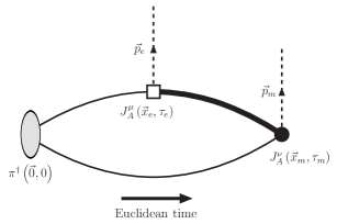
Figure 2: A diagram of the three-point correlator used in this calculation with current insertions at times $\tau_{e}$ and $\tau_{m}$.

For $0\ll\tau\ll T$, the 2-point correlator is saturated with the contribution of the lowest-lying hadronic state and can be written as

$$C_{2}(\tau,\mathbf{p})\sim\frac{|Z_{\pi}(\mathbf{p})|^{2}}{2E_{\pi}(\mathbf{p})}\left[e^{-E_{\pi}(\mathbf{p})\tau}+e^{-E_{\pi}(\mathbf{p})(T-\tau)}\right]\,,$$ (26)

which allows determination of the overlap factor $Z_{\pi}(\mathbf{p})=\langle 0|\mathcal{O}_{\pi}|\pi(\mathbf{p})\rangle$ and the pion energy $E_{\pi}(\mathbf{p})$.

Similarly, for $0\ll\tau_{e},\tau_{m}\ll T/2$, the 3-point correlation function takes the form

$$C_{3}^{\mu\nu}(\tau_{e},\tau_{m};\mathbf{p}_{e},\mathbf{p}_{m})\sim R^{\mu\nu}(\tau;\mathbf{p},\mathbf{q})\frac{Z_{\pi}(\mathbf{p})}{2E_{\pi}(\mathbf{p})}e^{-E_{\pi}(\mathbf{p})(\tau_{e}+\tau_{m})/2}\,,$$ (27)

with $\mathbf{p}=\mathbf{p}_{e}+\mathbf{p}_{m}$ and $\tau=\tau_{e}-\tau_{m}$, allowing one to extract

$$R^{\mu\nu}(\tau;\mathbf{p},\mathbf{q})=\frac{2E_{\pi}(\mathbf{p})C_{3}^{\mu\nu}(\tau_{e},\tau_{m};\mathbf{p}_{e},\mathbf{p}_{m})}{Z_{\pi}(\mathbf{p})e^{-E_{\pi}(\mathbf{p})(\tau_{e}+\tau_{m})/2}}$$ (28)

from the two- and three-point correlators. From this and Eq. (21) and (23), one can extract the second Mellin moment on the lattice.

IV Details of numerical implementation

IV.1 Lattice Action and $\mathcal{O}(a)$ Improvements

Order-$a$ corrections to correlation functions arise from both the action and the interpolating operators Symanzik (1983a, b); Luscher et al. (1996). Thus in order to remove these effects, one must in general improve both. The ensembles were generated with the standard Wilson gauge action

$$S_{G}[\psi,\overline{\psi},U] =\frac{\beta}{3}\sum_{n}\sum_{\mu<\nu}\text{Re}\left\{\text{Tr}\left[1-P_{\mu\nu}(n)\right]\right\}\,,$$ (29)

where $\beta=6/g^{2}$ is inverse coupling and $P_{\mu\nu}$ is the Wilson plaquette. The gauge action is automatically $\mathcal{O}(a)$ improved.

The Wilson fermion action, which is omitted from ensemble generation in the quenched approximation but is used in propagator construction, is given by

$$S_{F}[\psi,\overline{\psi},U] =a^{4}\sum_{f=1}^{N_{f}}\sum_{m,n}\overline{\psi}^{(f)}_{\alpha a}(n)\left[\frac{1}{2a\kappa^{(f)}}\delta_{\alpha\beta}\delta_{ab}\delta_{nm}-\frac{1}{2a}\sum_{\mu=\pm 1}^{\pm 4}(1-\gamma_{\mu})_{\alpha\beta}U_{\mu}(n)_{ab}\delta_{n+\hat{\mu},m}\right]\psi^{(f)}_{\beta b}(m)\,,$$ (30)

where $\kappa^{(f)}$ is the hopping parameter for flavour $f$ Gatringer and Lang (2010). The fermion action can be improved by addition of the clover term

$$\delta S[\overline{\psi},\psi,U]=\frac{1}{4}a^{5}c_{\text{sw}}\sum_{n}\sum_{\mu\nu}\overline{\psi}(n)i\sigma^{\mu\nu}\hat{F}_{\mu\nu}(n)\psi(n)\,,$$ (31)

where $\sigma_{\mu\nu}=\left[\gamma_{\mu},\gamma_{\nu}\right]/2i$ and $\hat{F}_{\mu\nu}$ is a discretized version of the field strength tensor corresponding to a sum over plaquettes. The clover coefficient $c_{\text{sw}}$ is taken from the non-perturbative tuning in Ref. Lüscher et al. (1997).

The $\mathcal{O}(a)$-improved, renormalized axial current operator is given by

$$J_{A}^{\mu}=Z_{A}^{(0)}(1+\tilde{b}_{A}a\tilde{m}_{ij})\left[\overline{\psi}\gamma_{\mu}\gamma_{5}\Psi+ac_{A}\partial_{\mu}\overline{\psi}\gamma_{5}\Psi-a\frac{c_{A}^{\prime}}{4}\left(\overline{\psi}\gamma_{\mu}\gamma_{5}(\overrightarrow{D}+m_{\Psi})\Psi-\overline{\psi}(\overleftarrow{D}+m_{\psi})\gamma_{\mu}\gamma_{5}\Psi\right)+\left(\psi\leftrightarrow\Psi\right)\right]\,,$$ (32)

where $Z_{A}^{(0)}$ is the axial-vector renormalization constant calculated in the chiral limit, $\tilde{m}_{ij}=(\tilde{m}_{i}+\tilde{m}_{j})/2$ is the average value of the masses of the two quark fields and $\tilde{b}_{A},c_{A},c_{A}^{\prime}$ are couplings which must be tuned to remove the $\mathcal{O}(a)$ corrections Bhattacharya et al. (2006). However, only $b_{A}$ is required for the $\mathcal{O}(a)$ improvement of the hadronic matrix element considered in this work.

This work studies the antisymmetric correlator $R^{[\mu\nu]}(\tau,\mathbf{p},\mathbf{q})$, which may be obtained by taking the antisymmetric combination of Eq. (22). For this specific matrix element, it is possible to show that the term proportional to $ac_{A}$ vanishes by symmetry (see Appendix A.2 for details). The terms proportional to $c_{A}^{\prime}$ can also be shown to vanish; details of this argument are given in Appendix A.3. This means that both renormalization and $\mathcal{O}(a)$ improvement of the current are, for the purposes of this work, purely multiplicative effects. $Z_{A}^{(0)}$ is given in Ref. Lüscher et al. (1997) and $\tilde{b}_{A}$ is given in Ref. Bhattacharya et al. (2006). However, in the time-momentum representation analysis procedure described below, any multiplicative factors only affect the fitted pion decay constant $f_{\pi}$ and not the second moment $\langle\xi^{2}\rangle$, and thus the second moment is independent of any uncertainties in these $\mathcal{O}(a)$ improvement parameters. As a result, lattice artifacts in $\langle\xi^{2}\rangle$ only enter at $\mathcal{O}(a^{2})$ or higher order.

IV.2 Lattice Parameters

Despite the $\mathcal{O}(a)$-improvement scheme described above, the method in this work requires very fine lattice spacings because of the large mass used for the intermediate heavy quark propagator. With renormalized heavy quark masses ranging from about 2 GeV to 4.5 GeV, lattice spacings between 0.08 fm and 0.04 fm are needed to keep $am_{\Psi}\lesssim 1$. At larger values of $am_{\Psi}$, lattice artifacts were uncontrolled and could not be reliably removed.

Due to critical slowing down, generating dynamical configurations at such fine spacings is expensive and beyond the scope of this preliminary study. As a result, this analysis uses gauge configurations generated in the quenched approximation following the multiscale procedure of Ref. Detmold and Endres (2018). The lattice spacings for the ensembles with $L/a=$ 24, 32, and 48 had previously been determined in Ref. Detmold and Endres (2018) using Wilson flow with a reference scale of $w_{0.4}=0.193$ fm Asakawa et al. (2015). This scale-setting procedure was repeated for the ensemble with $L/a=40$. The lattice geometries were tuned to a constant physical volume of 1.92 fm, which was kept small to reduce computational costs.

Finite volume effects were suppressed by using light quark masses tuned to give $m_{\pi}\approx 550$ MeV so that $m_{\pi}L\approx 5.3$. The heavy quark masses were chosen to give approximately constant masses of the heavy-heavy pseudoscalar meson across the four lattices. Details on the lattices and quark masses used are listed in Table 1. The required 2- and 3-point functions were generated using the software package Chroma with the QPhiX inverters Edwards and Joó (2005); Joó et al. (2016).

$(L/a)^{3}\times T/a$	$\beta$	$a$ (fm)	$\kappa_{\text{light}}$	$\kappa_{\text{heavy}}$	$c_{\text{sw}}$	Configurations Used	Sources/Config	Total Sources Used
$24^{3}\times 48$	6.10050	0.0813	0.134900	$\begin{matrix}0.1200\\ 0.1100\end{matrix}$	1.6842	650	12	7800
$32^{3}\times 64$	6.30168	0.0600	0.135154	$\begin{matrix}0.1250\\ 0.1184\\ 0.1095\end{matrix}$	1.5792	450	10	4500
$40^{3}\times 80$	6.43306	0.0502	0.135145	$\begin{matrix}0.1270\\ 0.1217\\ 0.1150\\ 0.1088\end{matrix}$	1.5292	250	6	1500
$48^{3}\times 96$	6.59773	0.0407	0.135027	$\begin{matrix}0.1285\\ 0.1244\\ 0.1192\\ 0.1150\\ 0.1100\end{matrix}$	1.4797	341	10	3410

Table 1: Details of the ensembles used in this numerical study.

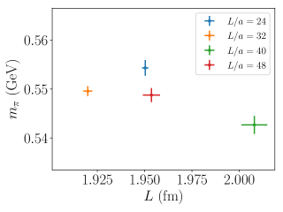
Figure 3: A comparison of tuning of pion mass and lattice spatial extent $L$ across the used ensembles.

IV.3 Choice of Heavy-Quark Masses

The operator product expansion in Eq. (21) will require higher-twist corrections that scale like $\Lambda_{\text{QCD}}/\tilde{Q}$ or $m_{\pi}/\tilde{Q}$. Unlike light-quark operator product expansions that rely on large momenta or small distances to suppress higher-twist effects Bali et al. (2018b), this work relies on the heavy intermediate mass for this suppression. With $m_{\Psi}\gtrsim q_{4}\gg|\mathbf{q}|$, higher-twist effects will scale as $\Lambda_{\text{QCD}}/m_{\Psi}$ or $m_{\pi}/m_{\Psi}$, so this analysis requires $\Lambda_{\text{QCD}},m_{\pi}\ll m_{\Psi}$. Separately, lattice artifacts enter as powers of either $a\Lambda_{\text{QCD}}$ or $am_{\Psi}$. Suppressing these will require $am_{\Psi}\lesssim 1$, so altogether it is required that

$$\Lambda_{\text{QCD}},m_{\pi}\ll m_{\Psi}\lesssim a^{-1}\,.$$ (33)

With $\Lambda_{\text{QCD}}\sim 250$ MeV and $m_{\pi}\approx 550$ MeV, $m_{\Psi}>1.8$ GeV provides some suppression of higher twist effects. To fit the residual higher-twist effects away will require a range of heavy quark masses, and therefore this analysis will consider $m_{\Psi}$ as large as 4.5 GeV. The lattice spacing is small enough for the finest discretization to accommodate such a heavy mass while maintaining $am_{\Psi}<1$; coarser lattices out of necessity have a smaller range of heavy quark masses. Figure 4 shows the quark masses used on each of the four ensembles considered here.

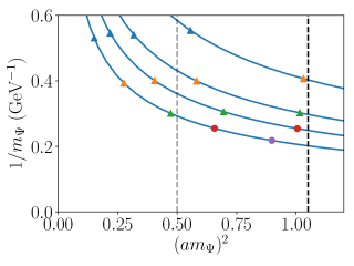
Figure 4: The four lattice spacings and the heavy quark masses used. The plot shows the trade-off between discretization effects (which can depend on $(am_{\Psi})^{2}$) and higher-twist effects (which scale as $1/m_{\Psi}$). At fixed lattice spacing, one can decrease the higher twist effects at the cost of increasing discretization errors, and the available trade-offs at the four lattice spacings studied here are shown by the blue curves. The coloured points show the masses actually used in this study. The black dashed line at $am_{\Psi}=1.05$ shows the cutoff beyond which discretization effects were no longer found to be well controlled, and the gray line at $am_{\Psi}=0.7$ shows a more conservative threshold used for analysing systematic errors arising from lattice artifacts.

IV.4 Choice of Kinematics

The heavy-quark OPE is given by

$$V^{[\mu\nu]}=-\frac{2if_{\pi}\varepsilon_{\mu\nu\rho\lambda}q^{\rho}p^{\lambda}}{\tilde{Q}^{2}}\left[C_{W}^{(0)}+\langle\xi^{2}\rangle\tilde{\omega}^{2}\left(1-\frac{p^{2}q^{2}}{6(p\cdot q)^{2}}\right)C_{W}^{\left(2\right)}+\cdots+\mathcal{O}\left(\frac{\Lambda_{\text{QCD}}}{\tilde{Q}}\right)\right]\,,$$ (34)

where $p$ is the momentum of the incoming pion and $q$ is the difference in momenta between the two outgoing currents, and where the ellipsis represents the contributions of higher moments that are negligibly small in this analysis. The exact form of the higher-twist effects suppressed by $\Lambda/\tilde{Q}$ is not known, but symmetries (see Appendix A.1) constrain it to be proportional to $\varepsilon_{\mu\nu\rho\lambda}q^{\rho}p^{\lambda}$.

In order to enhance the contribution of the second moment, one would like its prefactor to be as large as possible. However, $\tilde{Q}^{2}$ must be large to suppress higher twist effects, and $\mathbf{p}$ is limited by noise that grows exponentially with the pion energy on the lattice. In this work, $\mathbf{\hat{p}}\equiv\frac{\mathbf{p}}{2\pi/L}$ was constrained to be one unit of momentum, which for the volumes used in this work corresponds to $|\mathbf{p}|=$ 640 MeV. At these kinematics, the second moment is a small contribution to the hadronic tensor. As such, it is desirable to isolate its effect from the much larger contribution of the zeroth moment. In this study, the axial current indices are fixed to be $\mu=1,\nu=2$, the prefactor on the right-hand side of Eq. (34) becomes

$$i\varepsilon_{\mu\nu\rho\sigma}q^{\rho}p^{\sigma}=i\left(q^{0}p^{3}-p^{0}q^{3}\right)=-q^{4}p^{3}-iE_{\pi}q^{3}\,.$$ (35)

If the kinematics are chosen such that $p^{3}=0$, then this prefactor is purely imaginary. At tree level, the entire contribution of the zeroth moment will be pure imaginary as well. However, $p\cdot q=iE_{\pi}q^{4}-\mathbf{p}\cdot\mathbf{q}$ is generically complex (as long as $\mathbf{p}\cdot\mathbf{q}\neq 0$), so the contribution of the second moment to the hadronic tensor will have nonzero real part. The effect of these special kinematics is shown in Fig. 5. This work met these criteria by choosing

$$\mathbf{\hat{p}}=(1,0,0)~{}~{}\text{and}~{}~{}\mathbf{\hat{q}}=(1/2,0,1)$$ (36)

in units of $2\pi/L$, as well as all combinations of $\mathbf{\hat{p}},\mathbf{\hat{q}}$ that are equivalent under lattice symmetries. With these choices, $\langle\xi^{2}\rangle$ can be extracted as the leading contribution in the real part of $V^{\mu\nu}$. (Note that $\mathbf{\hat{q}}=(\mathbf{\hat{p}}_{m}-\mathbf{\hat{p}}_{e})/2$, so it is quantized in half-integers rather than integers.)

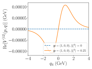
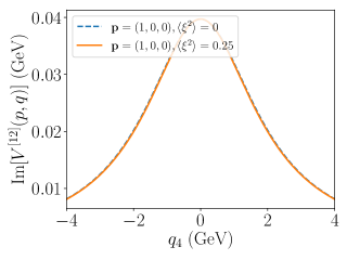
Figure 5: Investigation of optimal kinematics for the HOPE procedure. Feasible lattice simulations are restricted to small lattice momentum, and thus for the HOPE method, small $\tilde{\omega}$. Generally speaking, this results in moments beyond the leading zeroth moment being highly suppressed. This behaviour may be seen in the imaginary part of the amplitude where the variation of $\expectationvalue{\xi^{2}}$ has minimal effect on the matrix element. By choosing $\hat{\mathbf{p}}=(1,0,0)$ and $\hat{\mathbf{q}}=(1/2,0,1)$, it is possible to show that the leading contribution to the real component of the amplitude arises from $\expectationvalue{\xi^{2}}$. Thus this choice of kinematics offers improved access to the second Mellin moment.

There are two caveats to this argument:

1. The Wilson coefficient of the zeroth moment $C_{W}^{(0)}$, while real at tree level, becomes complex at 1-loop order and also contributes to the real part of $V^{\mu\nu}$. However, this contribution is suppressed by $\alpha_{s}$, and it is known analytically, so this small correction can be subtracted.

2. Higher-twist contributions may also be complex, but their contribution to $\text{Re}[V^{\mu\nu}]$ must also contain powers of $(p\cdot q)^{2}/(\tilde{Q}^{2})^{2}$, just like the second moment contribution. They are further suppressed by $\Lambda_{\text{QCD}}/\tilde{Q}$, so it is expected that they are smaller than the second moment contribution, particularly for large $\tilde{Q}^{2}$.

However, assuming the second Mellin moment is $\langle\xi^{2}\rangle\sim 0.25$, both of the above contributions are subdominant at the special kinematics chosen here.

IV.5 Computing Real and Imaginary Parts of $V^{\mu\nu}$

To compute the hadronic tensor, values of $R^{\mu\nu}(\tau)\propto C_{3}^{\mu\nu}(\tau_{e},\tau_{m}=\tau_{e}+\tau)$ are needed at both positive and negative values of $\tau$. In particular, using the fact that $R^{\mu\nu}(\tau)$ is pure imaginary, the imaginary and real parts of $V^{\mu\nu}$ can be written in terms of symmetric and antisymmetric combinations of $R^{\mu\nu}(\pm\tau)$:

$$\text{Re}[V^{\mu\nu}(\mathbf{p},q)] =\int_{0}^{\infty}d\tau\,\left[R^{\mu\nu}(\tau;\mathbf{p},\mathbf{q})-R^{\mu\nu}(-\tau;\mathbf{p},\mathbf{q})\right]\sin(q_{4}\tau)\,,$$ (37)

$$\text{Im}[V^{\mu\nu}(\mathbf{p},q)] =\int_{0}^{\infty}d\tau\,\left[R^{\mu\nu}(\tau;\mathbf{p},\mathbf{q})+R^{\mu\nu}(-\tau;\mathbf{p},\mathbf{q})\right]\cos(q_{4}\tau)\,.$$ (38)

At the kinematics of interest, the real part of $V^{\mu\nu}$ is about two orders of magnitude smaller than the imaginary part, so computing the difference in Eq. (37) requires a delicate cancellation between $R^{\mu\nu}(\pm\tau)$. The computation becomes more tractable if the two terms are highly correlated, as this increases the statistical power of the correlated difference. These correlations are substantially enhanced if values of $C_{3}^{\mu\nu}$ for $\tau<0$ are obtained using the identity

$$C_{3}^{\mu\nu}(\tau_{e},\tau_{m};\mathbf{p}_{e},\mathbf{p}_{m})^{*}=C_{3}^{\nu\mu}(\tau_{m},\tau_{e};-\mathbf{p}_{m},-\mathbf{p}_{e})\,.$$ (39)

Then Eq. (37) and (38) can be written as

$$\text{Re}[V^{\mu\nu}(\mathbf{p},q)] =\int_{0}^{\infty}d\tau\,\left[R^{\mu\nu}(\tau;\mathbf{p},\mathbf{q})+R^{\mu\nu}(\tau;-\mathbf{p},\mathbf{q})\right]\sin(q_{4}\tau)\,,$$ (40)

$$\text{Im}[V^{\mu\nu}(\mathbf{p},q)] =\int_{0}^{\infty}d\tau\,\left[R^{\mu\nu}(\tau;\mathbf{p},\mathbf{q})-R^{\mu\nu}(\tau;-\mathbf{p},\mathbf{q})\right]\cos(q_{4}\tau)\,.$$ (41)

Consequently, one can obtain both $\tau>0$ and $\tau<0$ at the same sets of current insertion times, which will enhance the correlations. A demonstration of this reduction in statistical error is shown in Figure 6.

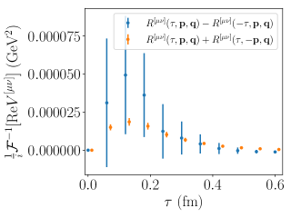
Figure 6: A comparison of the real part of the hadronic tensor computed using Eq. (37) versus Eq. (40), the latter of which has been manipulated to reduce the statistical error. While the manipulations do not change the expectation of the correlator, they reduce statistical uncertainties by about an order of magnitude. For comparison purposes, both quantities were measured on 2 sources on each of 450 configurations.

IV.6 Excited State Contamination and Choice of $\tau_{e}$

The three point correlator $C_{3}^{\mu\nu}(\tau_{e},\tau_{m})=\langle J_{A}^{\mu}(\tau_{e})J_{A}^{\nu}(\tau_{m})\mathcal{O}_{\pi}^{\dagger}(0)\rangle$ is computed by creating a pion source, propagating one of the quarks forward to $\tau_{e}$, creating a sequential source, and then tying together the sequential heavy-quark propagator and the other light quark propagator at the sink. Since $\tau_{e}\leq\tau_{m}$ is chosen in this work, excited state effects arise from the fact that the combination of states created by the pion interpolator have not fully relaxed to the ground state before $\tau_{e}$, so they are suppressed exponentially in $\tau_{e}$. Excited-state effects are reduced by using a Gaussian-smeared pion source Güsken (1990) with smearing radius equal to the inverse pion mass ($aw_{\text{smear}}=\left\{4.5,6.0,8.0,9.0\right\}$ for $L/a=\left\{24,32,40,48\right\}$, respectively). With this smearing, numerical study on the $L/a=32$ lattices showed that excited state contamination is estimated to be about 1% for a source-operator separation $\tau_{e}$ of about 0.7 fm, as shown in Figure 7.

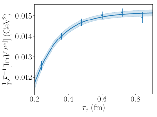
(a)

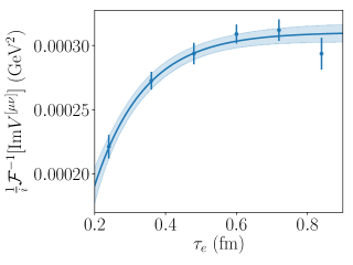
(b)

Figure 7: Excited state contamination at operator separations (a) $\tau=0.06$ fm and (b) $\tau=0.36$ fm.

Since $\tau_{e}$ must be fixed at runtime, $\tau_{e}\sim 0.7$ fm is chosen, leading to a $\sim 1\%$ systematic error due to excited-state contamination. Excited state contamination in the 2-point function is better controlled since one does not need to choose the source-sink separation at runtime, and one can afford the very conservative fit range of $\left[T/4,3T/4\right]$ since the statistical errors on the 2-point function are smaller than those on the 3-point function (for an example of the goodness of fit, see Fig. 8).

V Analysis, results and discussion

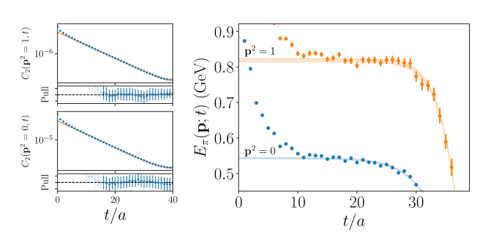
Figure 8: Validation plots for the single-state ansatz used in this study. The left panels show fits to the $L/a=40$ pseudoscalar correlator for $|\mathbf{p}|=1$ and $|\mathbf{p}|=0$, respectively, while the right panel shows the resulting effective mass plateaus. The “pull” in the left-hand plot is the residual of each data point normalized to the its standard deviation and is a measure of that point’s effect on the fit.

Extraction of the second moment from the 2- and 3-point correlation functions measured here is nontrivial due to signal contamination by both lattice artifacts and higher-twist effects. The extraction of $Z_{\pi}(\mathbf{p})$, $E_{\pi}(\mathbf{p})$ from fitting the 2-point correlation function $C_{2}(\tau,\mathbf{p})$ at late $\tau$ and the construction of $R^{\mu\nu}(\tau)$ in Eq. (22) are relatively straightforward. However, comparing the 3-point data to the OPE of the hadronic amplitude can be done in multiple ways, which can lead to somewhat different systematics. As this is the first numerical study of the HOPE method, two analysis methods, called the time-momentum analysis and the momentum-space analysis, are performed. This enables a cross-check of the results and ensures that they are robust against systematics in the analysis procedure. These analysis methods are as follows:

1. Time-momentum analysis

   1. Fit $f_{\pi}$ and the heavy quark mass $m_{\Psi}$ by comparing the symmetric part of the data to the inverse Fourier transform of the OPE of $\text{Im}[V(\mathbf{p},q)]$, that is, from the inverse Fourier transform of Eq. (41).

   2. Use the fitted results of $f_{\pi},m_{\Psi}$ and the antisymmetric part of the data to fit the second moment $\langle\xi^{2}\rangle$ from the inverse Fourier transform of $\text{Re}[V(\mathbf{p},q)]$, using Eq. (40), at each heavy quark mass and lattice spacing.

   3. Perform a combined fit to $\langle\xi^{2}\rangle(a,m_{\Psi})$ to remove both lattice spacing and higher-twist effects.

2. Momentum-space analysis

   1. Perform a Fourier transform of $R^{\mu\nu}(\tau)$ in the temporal direction.

   2. Extrapolate the momentum-space hadronic amplitude to the continuum.

   3. Fit $f_{\pi}$, $m_{\Psi}$ and $\expectationvalue{\xi^{2}}$ to the hadronic amplitude in the continuum limit using the momentum-space, continuum HOPE formula presented in Sec. III.1.

Figure 9: Comparing the two analysis strategies. Both approaches utilize the same bare correlators, but note that the order of the continuum extrapolation and HOPE fit are reversed.

These alternative procedures are shown diagrammatically in Fig. 9. The following sections will detail both analysis strategies.

V.1 Time-Momentum Analysis

The ratio $R^{\mu\nu}\left(\tau;\mathbf{p},\mathbf{q}\right)$ was constructed for $0<\tau\leq\tau_{\text{max}}\approx 0.6$ fm. The statistical quality of the signal deteriorates with time, and large-$\tau$ data may be more susceptible to higher-twist contamination, motivating the cut at $\tau_{\text{max}}$. The symmetric and anti-symmetric components of $R^{\mu\nu}(\tau)$ are constructed as described in Section II-B.

An example fit to $V^{\mu\nu}$ for a single heavy quark mass at a single lattice spacing is shown in Fig. 10. At the chosen kinematics, the second moment provides a negligible contribution to the imaginary part of the hadronic tensor (see Fig. 5), so the fitting procedure can be split into two steps: one in which $f_{\pi}$ and $m_{\Psi}$ are fit to the imaginary part of $V^{\mu\nu}$ and a second step that consists of a single-parameter fit of $\langle\xi^{2}\rangle$ to the real part of $V^{\mu\nu}$, where $f_{\pi}$ and $m_{\Psi}$ are used as inputs. At values of $\tau$ comparable to the lattice spacing, uncontrolled discretization effects are to be expected. Additionally, if the two current insertions are close in space-time relative to the lattice spacing, they may mix with lower-dimensional operators and lead to UV divergences. Both of these effects suggest that small-$\tau$ data should be removed from the fits. Empirically, the $\chi^{2}$ values for the fits to the various heavy-quark masses became reasonable if the $\tau\leq 2a$ data are excluded, so all fits will only use data with $\tau\geq 3a$.

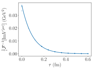
(a)

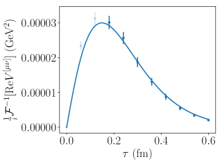
(b)

Figure 10: The real and imaginary parts of the hadronic tensor $V^{\mu\nu}$ can be inverse Fourier transformed (indicated by $\mathcal{F}^{-1}$) to produce the antisymmetric and symmetric components of the ratio of correlators $R^{\mu\nu}$. The symmetric part of $R^{\mu\nu}(\tau)$ (corresponding to $\mathcal{F}^{-1}[\text{Im}(V^{\mu\nu})]$) is dominated by the zeroth moment contribution, allowing extraction of $f_{\pi}$ and $m_{\Psi}$. These are then used as inputs to the fit of $\mathcal{F}^{-1}[\text{Re}(V^{\mu\nu})]$ to extract the second moment $\langle\xi^{2}\rangle$. In order to avoid contamination with UV divergences near $\tau=0$, points with $\tau<3a$ (grayed out in the plots) are excluded from the fit.

This fitting procedure compares lattice data to a continuum, twist-2 OPE. As a result, the extracted second moment $\langle\xi^{2}\rangle(a,m_{\Psi})$ will be contaminated by both lattice artifacts and higher-twist corrections. The lattice artifacts enter at $O(a^{2})$ (see Appendices A.2, A.3 for details), and by dimensional analysis, $a^{2}$ must be accompanied by two factors of a mass scale, either the typical momentum scale of $\Lambda_{\text{QCD}}$ or the heavy quark mass $m_{\Psi}$, so there may be discretization effects proportional to $a^{2}$, $a^{2}m_{\Psi}$, or $a^{2}m_{\Psi}^{2}$. With $am_{\Psi}<1.05$, these terms were sufficient to describe lattice artifacts without need for additional $O(a^{3})$ terms. Higher-twist effects scale as powers of $\Lambda_{\text{QCD}}/\tilde{Q}$ or $m_{\pi}/\tilde{Q}$, and $\Lambda_{\text{QCD}}\sim m_{\pi}$ in this analysis. The fitting procedure effectively integrates over the $q_{4}$ dependence, and $m_{\Psi}\gg|\mathbf{q}|$, so the twist-3 contribution can be approximated by a $\Lambda/m_{\Psi}$ term. Therefore, to extract $\langle\xi^{2}\rangle$ in the continuum limit without higher-twist contamination, $\langle\xi^{2}\rangle(a,m_{\Psi})$ is fit to the formula

$$\langle\xi^{2}\rangle(a,m_{\Psi})=\langle\xi^{2}\rangle+\frac{A}{m_{\Psi}}+Ba^{2}+Ca^{2}m_{\Psi}+Da^{2}m_{\Psi}^{2}\,,$$ (42)

where $\langle\xi^{2}\rangle$, $A$, $B$, $C$, and $D$ are the fit parameters. At an intermediate mass scale of $m_{\Psi}=3$ GeV and a lattice spacing of $a=0.06$ fm, the magnitudes of the various terms are

$$\langle\xi^{2}\rangle =0.210\pm 0.013,$$ (43)

$$\frac{A}{m_{\Psi}} =0.009\pm 0.005,$$ (44)

$$Ba^{2} =-0.004\pm 0.013,$$ (45)

$$Ca^{2}m_{\Psi} =-0.004\pm 0.013,$$ (46)

$$Da^{2}m_{\Psi}^{2} =-0.027\pm 0.006,$$ (47)

where the renormalization scale for $\langle\xi^{2}\rangle$ is taken to be $\mu=2$ GeV and the error bars are purely statistical. Neither the higher-twist nor the discretization effects can be neglected at the precision considered in this work. The fit result for $\langle\xi^{2}\rangle$ is shown in Figure 11.

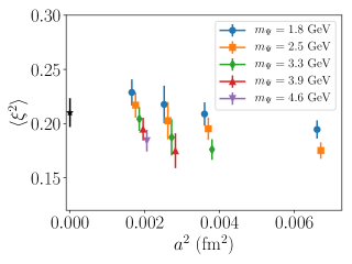
Figure 11: The values of $\langle\xi^{2}\rangle(a,m_{\Psi})$ at the gauge couplings and heavy quark masses listed in Table 1, plotted as a function of $a^{2}$ with the heavier masses at each lattice spacing displaced slightly to the right for visual clarity. The black star at $a^{2}=0$ represents the extrapolated value from the fit to Eq. (42).

V.2 Estimation of Systematic Uncertainties for Time-Momentum Analysis

The analysis procedure described in the previous subsection contains several systematic errors. Excited state contamination in the 3-point function was estimated in Sec. IV.6 to be a $\sim 1\%$ effect (and contamination in the 2-point function is much smaller). Finite-volume effects are expected to scale as $\frac{1}{m_{\pi}L}e^{-m_{\pi}L}<10^{-3}$ and are negligible compared to both statistical and other systematic errors.

This work uses an unphysically heavy pion mass of $m_{\pi}\sim 550$ MeV. Previous studies Braun et al. (2015) have indicated that $\langle\xi^{2}\rangle$ at such a pion mass differs from its physical value by about $5\%$. Therefore, this is taken as a systematic effect arising from the unphysical pion mass.

Other systematic errors can be estimated by studying the effects of changing input parameters or varying the analysis procedure.

• The global fit described in Eq. (42) restricted the heavy quark masses to those satisfying $am_{\Psi}<1.05$. To test whether this cut is sufficient to exclude lattice artifacts of $O(a^{3})$ or higher, one could choose a more conservative cut, using only data satisfying $am_{\Psi}<0.7$. Refitting with this more limited data set results in a fit value of $\langle\xi^{2}\rangle=0.226\pm 0.043$. Although these two results are compatible within one standard deviation, the difference between the central values (0.016) is taken as the estimate of the systematic uncertainty from the continuum extrapolation.

• The global fit contains a $\Lambda_{\text{QCD}}/m_{\Psi}$ term to account for the twist-3 contribution. In principle, higher-twist contributions are also present. To estimate such systematic effects, one could add a $\Lambda_{\text{QCD}}/m_{\Psi}^{2}$ term to the global fit in Eq. (42). This changes the fit result to $\langle\xi^{2}\rangle=0.185\pm 0.017$ which has a central value differing from that of the primary procedure by 0.025. This is taken to be the systematic uncertainty from higher twist effects.

• As explained in Sec. V.1, at small values of $\tau=\tau_{m}-\tau_{e}$, the data are contaminated with uncontrolled lattice artifacts. The primary fit omits the $\tau/a=0$, 1, and 2 points, where such effects are the most significant and result in unacceptable $\chi^{2}$ values in the fits. To analyse errors arising from the placement of this cut, one can exclude $\tau/a=3$ from the fits, which gives a modified result of $\langle\xi^{2}\rangle=0.208\pm 0.014$ and therefore a small systematic uncertainty from the difference in central values of 0.002.

• The Wilson coefficients $C_{W}$ are calculated in perturbation theory, and in this analysis, they are only computed to 1-loop order. As an estimate of the magnitude of higher-loop corrections, one can perform this analysis at a larger renormalization scale of $\mu=4$ GeV and then run back to $\mu=2$ GeV using Eq. (4). Such a procedure results in $\langle\xi^{2}\rangle(\mu=4\text{ GeV})=0.216\pm 0.012$, which evolves to $\langle\xi^{2}\rangle(\mu=2\text{ GeV})=0.218\pm 0.014$, giving a systematic uncertainty of 0.008 from the change in central value.

The above procedure for estimating systematic effects leads to a final value of $\langle\xi^{2}\rangle(\mu=2\text{ GeV})=0.210\pm 0.013\text{ (stat.)}\pm 0.034\text{ (sys.)}$, which can be combined in quadrature to give $\langle\xi^{2}\rangle(\mu=2\text{ GeV})=0.210\pm 0.036$ (total, exc. quenching). The above error estimates are summarized in Table 2.

Source of error	Size
Statistical	0.013
Continuum extrapolation	0.016
Higher-twist	0.025
Excited-state contamination	0.002
Unphysical $m_{\pi}$	0.014
Fit range	0.002
Running coupling	0.008
Total (exc. quenching)	0.036

Table 2: The error budget for the computation of the second Mellin moment $\langle\xi^{2}\rangle$ using the HOPE method, with the data processed in the time-momentum representation.

The dominant sources of uncertainty are from the continuum and higher-twist extrapolations. In principle, both these extrapolations can be better controlled by including finer lattice spacings, which would also allow the inclusion of larger heavy-quark masses. However, computations at finer lattices are expensive and therefore beyond the scope of this preliminary work. The error from quenching is formally uncontrollable, although empirically it is a 10–20% effect in many calculations. To perform a precise comparison of this result to dynamical calculations would require redoing these calculations on dynamical ensembles.

V.3 Determination of $f_{\pi}$

The previous two subsections describe the determination of the second moment of the pion LCDA using the time-momentum analysis procedure. To check the validity of the HOPE strategy, it is worth noting that the pion decay constant $f_{\pi}$ is computed as a byproduct of this analysis. As is clear in the OPE formula, Eq. (21), $f_{\pi}$ is an overall normalization factor for the hadronic amplitude $V^{\mu\nu}$.

One can extrapolate the $f_{\pi}$ values computed at various heavy quark masses on the four ensembles to the continuum using the same procedure as for the extrapolation of $\langle\xi^{2}\rangle$, giving a global fit value of $161\pm 2$ MeV after removal of lattice discretization and higher-twist effects, where the error reflects statistical uncertainties only. It should be noted that this measurement suffers from not only the systematic errors mentioned in the previous subsection but also additional uncertainties from the normalization constants $Z_{A}$ and $\tilde{b}_{A}$ to which the second moment is completely insensitive in the time-momentum analysis.

On the other hand, $f_{\pi}$ can be directly measurable on the lattice via the axial-axial correlator at $0\ll\tau\ll T$,

$$\langle 0|A_{4}(\tau)A_{4}(0)|0\rangle\sim\frac{(f_{\pi}Z_{A})^{2}m_{\pi}}{2}\left[e^{-m_{\pi}\tau}+e^{-m_{\pi}(T-\tau)}\right]\,,$$ (48)

where $A_{4}$ is the local unsmeared axial current $\overline{\psi}\gamma_{4}\gamma_{5}\psi$ and the convention where $f_{\pi}\sim 130$ MeV at the physical pion mass is used. As written, Eq. (48) contains $O(a)$ corrections, so the continuum extrapolation must include a term linear in $a$ rather than in $a^{2}$. A low-statistics (one source per configuration) computation of $f_{\pi}$ at the four lattices gives a continuum value of $f_{\pi}=157\pm 6$ MeV.

Despite the systematics that could affect the value extracted from the hadronic tensor measurement, the two determinations of $f_{\pi}$ are in good agreement (see Fig. 12). While $f_{\pi}$ is not directly relevant to the calculation, this serves as a useful cross-check of the validity of the operator product expansion and, more generally, of this calculational method.

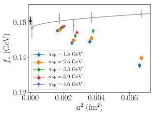
Figure 12: Extrapolation of $f_{\pi}$ to the continuum. The coloured points at finite lattice spacing are the values of $f_{\pi}$ extracted from the four lattice spacings at various heavy quark masses as an intermediate step in the determination of $\langle\xi^{2}\rangle$. The black point is the global fit of $161\pm 2$ MeV to the hadronic tensor data. The gray points are direct computations of $f_{\pi}$ at the four lattice spacings. These direct calculations suffer from $O(a)$ discretization errors, but an extrapolation linear in $a$ gives a continuum value of $158\pm 5$ MeV, in good agreement with the value extracted from hadronic tensor measurements.

V.4 Momentum-Space Analysis

A further check of the validity of the time-momentum representation method can be obtained by analysing the same data using a momentum-space analysis. The starting point for the momentum-space analysis is the time-momentum representation ratio $R^{[\mu\nu]}(\tau,\mathbf{p},\mathbf{q};a)$ constructed in Eq. (28). The lattice-regularized data are converted to momentum-space via

$$V^{[\mu\nu]}(p,q;a)=a\sum_{\tau=-\tau_{\text{max}}}^{\tau_{\text{max}}}e^{i\tau q_{4}}R^{[\mu\nu]}(\tau,\mathbf{p},\mathbf{q};a)\,,$$ (49)

where $\tau_{\text{max}}$ was taken to be approximately $1\mbox{ fm}=5\mbox{ GeV}^{-1}$. By Fourier transforming the tree-level HOPE equation, it is possible to show that the numerical data decay exponentially in $\tau$ as

$$R^{[\mu\nu]}(\tau,\mathbf{p},\mathbf{q};a)\sim\frac{e^{-E_{\mathbf{q}}\tau}}{2E_{\mathbf{q}}}\,,$$ (50)

where $E_{\mathbf{q}}=\sqrt{m_{\Psi}^{2}+\mathbf{q}^{2}}$. Since $R^{[\mu\nu]}(\tau,\mathbf{p},\mathbf{q};a)$ exhibits exponential decay in $\tau$ with an exponent with magnitude greater than approximately $2\mbox{ GeV}$, the truncation in the sum in Eq. (49) is expected to be well controlled. While the discrete Fourier transform formally only produces a discrete set of Fourier modes, in this work, interpolation between these Fourier modes is achieved by evaluating Eq. (49) for arbitrary $q_{4}$. Note that the largest Fourier mode, $q_{4}^{\text{max}}$ must be taken sufficiently small to remain below the Nyquist frequency which corresponds to requiring $q_{4}^{\text{max}}<\pi/a$. For the ensemble with the coarsest lattice spacing ($a=0.0813\mbox{ fm}$) this results in the constraint that $q_{4}^{\text{max}}<7.5\mbox{ GeV}$. In practice, data at momenta close to the Nyquist frequency may possess large lattice artifacts, and in this analysis $q_{4}^{\text{max}}=5\mbox{ GeV}$ is chosen.

While data at non-zero $\tau$ are guaranteed to have a well-defined continuum limit, $\tau=0$ data contain additional UV divergences arising from the mixing of the current-current operator with lower-dimensional operators. After performing the Fourier transform, this divergence will appear as an additive shift in the numerical data. Thus in order to ensure that the hadronic amplitude considered in this work has a well-defined continuum limit (after finite, multiplicative renormalization), a single subtraction is first performed at fixed lattice spacing:

$$V_{\text{sub}}^{[\mu\nu]}(p,q;a)=V^{[\mu\nu]}(p,q;a)-V^{[\mu\nu]}\left[p,(\mathbf{q},q_{4,\text{sub}});a\right]\,,$$ (51)

where $q_{4,\text{sub}}$ is chosen to be $q_{4,\text{sub}}=q_{4}^{\text{max}}=5\mbox{ GeV}$. This choice is informed by the desire to minimize the statistical noise introduced in this process. As a result of this subtraction, the matrix element may be expressed generically as

$$V_{\text{sub}}^{[\mu\nu]}(p,q;a)=\sum_{n=0}^{\infty}a^{n}V_{(n),\text{sub}}^{[\mu\nu]}(p,q)\,,$$ (52)

where $V_{(0),\text{sub}}^{[\mu\nu]}(p,q)\equiv V_{\text{sub}}^{[\mu\nu]}(p,q)$ is the continuum hadronic matrix element. As emphasized previously, the simplicity of this continuum limit is one of the advantages of considering a current-current correlator. As argued in Sec. IV.1, it is possible to show that the use of the the Sheikholeslami-Wohlert (clover) improved action leads to the removal of $\mathcal{O}(a)$ corrections for the matrix element studied here (see Appendices A.2, A.3 for details), so

$$V_{\text{sub}}^{[\mu\nu]}(p,q;a)=V_{\text{sub}}^{[\mu\nu]}(p,q)+a^{2}V_{(2),\text{sub}}^{[\mu\nu]}(p,q)+\mathcal{O}(a^{3})\,.$$ (53)

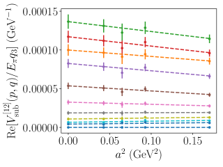
(a)

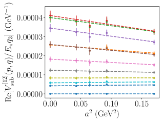
(b)

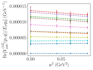
(c)

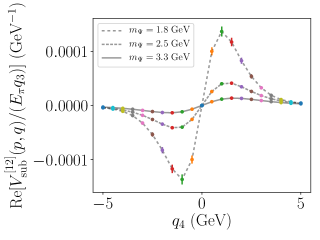
(d)

Figure 13: Continuum extrapolation of real part of hadronic matrix element. Figs. 13a - 13c show the pointwise continuum extrapolation for each value of $q_{4}$ for heavy quark masses of (a) $m_{\Psi}=1.8\mbox{ GeV}$, (b) $m_{\Psi}=2.5\mbox{ GeV}$, and (c) $m_{\Psi}=3.3\mbox{ GeV}$. The resulting hadronic amplitude in the continuum is shown in Fig. 13d, where curves are included to guide the eye.

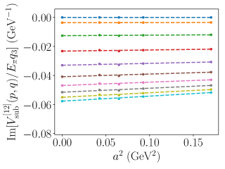
(a)

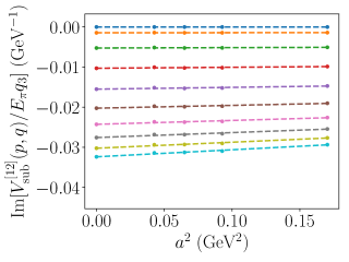
(b)

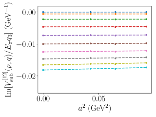
(c)

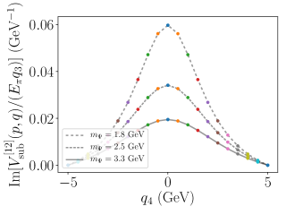
(d)

Figure 14: Continuum extrapolation of imaginary part of hadronic matrix element. Figs. 14a - 14c show the pointwise continuum extrapolation for each value of $q_{4}$ for heavy quark masses of (a) $m_{\Psi}=1.8\mbox{ GeV}$, (b) $m_{\Psi}=2.5\mbox{ GeV}$, and (c) $m_{\Psi}=3.3\mbox{ GeV}$. The resulting hadronic amplitude in the continuum is shown in Fig. 14d, where curves are included to guide the eye.

It is important to note that the continuum extrapolation requires taking $a\to 0$ along a line of constant physics. This is achieved by tuning the bare parameters to ensure certain physical quantities remain fixed as lattice spacing is varied, but there are some mistunings resulting from percent level inaccuracies in the tuning process. While such a mistuning appears as a relatively mild effect in the time-momentum representation analysis where it results in a variation of $f_{\pi}$, the momentum-space approach is more sensitive to any such mistuning, since it affects the continuum extrapolation of the hadronic matrix element $V^{[\mu\nu]}(p,q)$. Evidence of this mistuning can be seen in Fig. 3. It is important to note that the tuning of the light-quark sector parameters to their physical values is an issue for all methods, and is not unique to this approach. One can reduce the systematic error associated with this mistuning by considering a ratio which is less sensitive to the volume and pion mass dependence. Examining the HOPE, the leading volume and pion mass dependent quantities are found in the prefactor (for $\mu=1$, $\nu=2$)

$$V_{\text{sub}}^{[12]}(p,q)\propto\epsilon^{12\alpha\beta}p_{\alpha}q_{\beta}\propto(E_{\pi}q_{3})\,,$$ (54)

for the special kinematics considered. In order to reduce the volume and pion mass dependence, the ratio $V_{\text{sub}}^{[12]}(p,q)/(E_{\pi}q_{3})$ is formed and then continuum extrapolated.

In contrast to the time-momentum representation analysis, a further cut must be made on the data included in the analysis. All data presented in the time-momentum representation analysis satisfy the constraint $am_{\Psi}<1.05$. This restriction is placed to ensure control over lattice artifacts. However, in addition to this constraint, the momentum-space analysis requires data at a sufficient number of lattice spacings for the continuum extrapolation to be performed. In particular, the model for the continuum extrapolation contains two free parameters, and thus the analysis must be limited to the subset of data where the the heavy quark mass satisfies the constraint $am_{\Psi}<1.05$ for at least three lattice spacings. From Fig. 4, this criterion constrains this analysis to make use of only the lightest three heavy quark masses. The continuum extrapolations of the real and imaginary parts of the hadronic amplitude are shown in Figs. 13, 14.

V.5 Extraction of Second Moment

Having extrapolated the real and imaginary parts of the hadronic matrix element to the continuum, a global fit is performed to the order-$\alpha_{S}$ HOPE formula given in Eq. (21) plus an additional twist-three ansatz which is used to control the leading higher-twist effects. The functional form of the model used in the extraction of the Mellin moments from the continuum data is

$$\begin{split}V^{[12]}(q,p,m_{\Psi})/(E_{\pi}q_{3})=&-\frac{2if_{\pi}}{\tilde{Q}^{2}}\left\{C_{W}^{(0)}(\tilde{Q}^{2},\mu,\tau)+C_{W}^{(2)}(\tilde{Q}^{2},\mu,\tau)\langle\xi^{2}\rangle\left[\frac{\zeta^{2}C_{2}^{2}(\eta)}{12\tilde{Q}^{2}}\right]\right\}\\ &+\frac{2if_{\pi}\Lambda_{\text{QCD}}}{\tilde{Q}^{3}}\left\{b_{0}+b_{2}\left[\frac{\zeta^{2}C_{2}^{2}(\eta)}{12\tilde{Q}^{2}}\right]\right\}\,.\end{split}$$ (55)

It is important to note that while the above parameterization of the twist-three piece is the most natural, other terms like $m_{\Psi}/\tilde{Q}^{4}$ are also possible. The resulting fit is shown in Fig. 15. As a result of this global analysis, the first two moments of the pion LCDA are found to be $f_{\pi}=0.173\pm 0.001\mbox{ GeV}$, and $\expectationvalue{\xi^{2}}(\mu=2\mbox{ GeV}^{2})=0.210\pm 0.013$, where the statistical uncertainty is determined from a bootstrap analysis of the numerical data. Since this a global fit, the three heavy quark masses are also determined to be $m_{\Psi}^{(1)}=1.82\pm 0.02\mbox{ GeV}$, $m_{\Psi}^{(2)}=2.52\pm 0.02\mbox{ GeV}$ and $m_{\Psi}^{(3)}=3.34\pm 0.02\mbox{ GeV}$, which are in good agreement with the heavy-quark masses determined at fixed lattice spacing in the time-momentum representation.

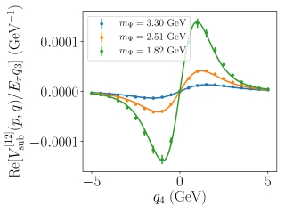
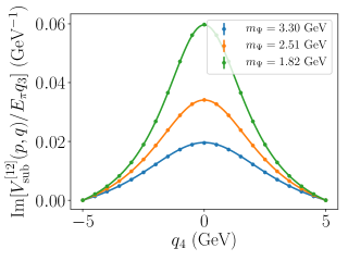
Figure 15: Global fit of continuum matrix element data to the HOPE formula to extract $f_{\pi}$, $m_{\Psi}$ and $\expectationvalue{\xi^{2}}$.

Systematic uncertainties in $\langle\xi^{2}\rangle$ for the momentum-space analysis may also be estimated following the same procedure as described in the time-momentum representation analysis. Since both analyses use the same lattice data they share some sources of systematic error. Thus the excited state contamination is taken to be a $\sim 1\%$ effect, and as with the time-momentum representation analysis, finite-volume effects are taken to be negligible. Finally, as in the time-momentum representation analysis, the unphysically heavy pion mass is assumed to contribute a 5% systematic error. In addition to these shared sources of systematic uncertainty, the momentum-space method has several additional sources of systematic error. These arise from the difference in the order of steps of the analysis, and are discussed below:

• Following the procedure employed above, $\mathcal{O}(a^{3})$ effects are studied by making a more conservative cut on $am_{\Psi}$. In particular, the cut is chosen to be $am_{\Psi}<0.7$, which is consistent with the time-momentum representation. The resulting fit leads to a value for the second moment of $\expectationvalue{\xi^{2}}=0.222\pm 0.068$. Taking the differences of central values leads to a systematic error of $0.012$.

• The effects of higher-twist contributions may be studied by adding a twist-four ansatz to the continuum HOPE formula in Eq. (55). The form chosen is

  $$V_{\text{higher-twist}}^{[12]}(q,p,m_{\Psi})/(E_{\pi}q_{3})=V^{[12]}(q,p,m_{\Psi})/(E_{\pi}q_{3})+\frac{2if_{\pi}\Lambda_{\text{QCD}}^{2}}{\tilde{Q}^{4}}\left\{c_{0}+c_{2}\left[\frac{\zeta^{2}C_{2}^{2}(\eta)}{12\tilde{Q}^{2}}\right]\right\}\,,$$ (56)

  mirroring the choice for the twist-three term. The resulting value for the second moment is $\expectationvalue{\xi^{2}}=0.245\pm 0.019$. This results in a systematic uncertainty of $0.035$.

• The higher-loop corrections to the Wilson coefficients are studied by repeating the above analysis at a renormalization scale of $\mu=4\mbox{ GeV}$, and then evolving back to $\mu=2$ GeV using the renormalization-group evolution of the Gegenbauer moments given by Eq. (4). This gives $\expectationvalue{\xi^{2}}(\mu=4\mbox{ GeV})=0.236\pm 0.016$. Running this to $2\mbox{ GeV}$ results in $\expectationvalue{\xi^{2}}(\mu=2\mbox{ GeV})=0.239\pm 0.017$. Taking the difference between the evolved $\expectationvalue{\xi^{2}}$ and the original fitted $\expectationvalue{\xi^{2}}(\mu=2\text{ GeV})$ gives a systematic uncertainty of $0.029$.

A breakdown of the sources of systematic error described here is given in Table 3. This analysis of systematic errors leads to a final value for the second moment of $\expectationvalue{\xi^{2}}(\mu=2\mbox{ GeV})=0.210\pm 0.013\text{(stat)}\pm 0.044\text{(syst)}$. These two sources of error may be added in quadrature to obtain the final result $\expectationvalue{\xi^{2}}(\mu=2\mbox{ GeV})=0.210\pm 0.046$. Similarly to the time-momentum space analysis, the dominant source of systematic uncertainty arises from the higher-twist terms. This issue is made worse in momentum-space due to the additional cut on lattice data required for the continuum extrapolation of the hadronic amplitude.

Source of error	Size
Statistical	0.013
Excited-state contamination	0.002
Continuum extrapolation	0.012
Higher-twist	0.035
Running coupling	0.029
Unphysical $m_{\pi}$	0.014
Total (exc. quenching)	0.046

Table 3: The error budget for the computation of the second Mellin moment $\langle\xi^{2}\rangle$ using the HOPE method, with the data analysed in the momentum-space approach.

V.6 Discussion of Results

The ratio $R^{[\mu\nu]}(\tau,\mathbf{p},\mathbf{q};a)$ was analysed using two alternative approaches, termed the time-momentum representation (TMR) analysis and the momentum-space (Mom) analysis. The results of the second moment from these approaches are

$$\expectationvalue{\xi^{2}}_{\text{TMR}}(\mu=2\mbox{ GeV}) =0.210\pm 0.013\text{ (stat.)}\pm 0.034\text{ (sys.)}=0.210\pm 0.036\,,$$ (57)

$$\expectationvalue{\xi^{2}}_{\text{Mom}}(\mu=2\mbox{ GeV}) =0.210\pm 0.013\text{ (stat.)}\pm 0.044\text{ (sys.)}=0.210\pm 0.046\,.$$ (58)

The central values and statistical errors are the same in both approaches. The agreement of central values is the result of statistical coincidence; with a different choice of fit parameters this extrapolated central value is expected to vary. The equivalence of the statistical error is relatively unsurprising, since both approaches mostly share the same raw lattice data.

As a cross-check, the pion decay constant $f_{\pi}^{\text{2pt}}=0.158\pm 0.005\mbox{ GeV}$ was extracted from a conventional analysis of the axial-vector 2-point correlation function. This is to be compared with the HOPE-derived values $f_{\pi}^{\text{TMR}}=0.161\pm 0.002\text{ (stat.)}\mbox{ GeV}$ and $f_{\pi}^{\text{Mom}}=0.173\pm 0.001\text{ (stat.)}\mbox{ GeV}$, with systematic uncertainties in $f_{\pi}$. The systematic uncertainties in these determinations $f_{\pi}$ are likely comparable to the systematic uncertainty in $\langle\xi^{2}\rangle$ (about 10-20%), or perhaps slightly larger due to the added uncertainty in the normalization factors.

Examining both procedures allows the study of the advantages and shortcomings of both approaches and serves as a further cross-check of the analysis. The above equations show that the time-momentum representation approach results in a smaller systematic error than that of the momentum-space analysis. While the systematic uncertainty incurred from the truncation of the twist expansion is the largest systematic error in both analyses, the additional cut placed on the data in the momentum-space analysis results in the removal of data with the heaviest heavy quark masses. Since higher-twist corrections are suppressed by factors of $1/\tilde{Q}\sim 1/m_{\Psi}$, this results in less control over the higher-twist effects.

Given the above considerations, the central value is chosen to be the more precise time-momentum representation analysis value of

$$\expectationvalue{\xi^{2}}(\mu=2\mbox{ GeV})=0.210\pm 0.036\,.$$ (59)

This corresponds to a Gegenbauer moment of

$$\phi_{2}(\mu=2\mbox{ GeV})=0.03\pm 0.11\,.$$ (60)

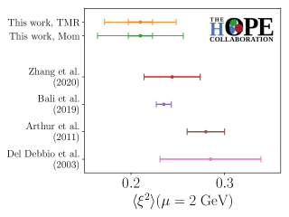
Figure 16: Comparison of $\langle\xi^{2}\rangle$ extracted from the time-momentum representation (TMR) and momentum-space analyses to various results in the literature. Note that the values from this work and Del Debbio et al. are in the quenched approximation, whereas the results from Zhang et al., Bali et al., and Arthur et al. use dynamical QCD, and the error bars do not reflect the uncertainty from the quenched approximation.

Most previous lattice calculations have used local operators to compute $\langle\xi^{2}\rangle$. In the quenched approximation, $\langle\xi^{2}\rangle$ was previously computed to be $0.280\pm 0.051$ at a renormalization scale of $\mu=2.67$ GeV Del Debbio et al. (2003). Running this down to 2 GeV gives $\langle\xi^{2}\rangle=0.285\pm 0.054$, which agrees with this quenched calculation, albeit with a large error bar.

More recent calculations with the local operator method have been performed in dynamical QCD, giving $\langle\xi^{2}\rangle=0.28\pm 0.02$ Arthur et al. (2011) and $\langle\xi^{2}\rangle=0.235\pm 0.008$ Bali et al. (2019b), both at $\mu=2$ GeV. A separate approach is to proceed via the quasi-distribution amplitude (the distribution amplitude analogue of the quasi-PDF), which was used to give a result of $\langle\xi^{2}\rangle=0.244\pm 0.030$ Zhang et al. (2020). These results are compared to the second moment determined in this work in Fig. 16. Formally, the uncertainty from quenching cannot be controlled, so a precise comparison of the results in this work to these dynamical calculations is not possible. However, in practice, quenching errors are usually at the order of 10–20%, and the calculation presented here agrees with the dynamical results within the listed uncertainties combined with this approximate quenching uncertainty.

VI Conclusion and outlook

Factorization theorems in QCD imply that the LCDA of the pion is relevant to a variety of experimental processes. Since the LCDA is a non-perturbative object, it is a quantity of importance for LQCD calculations. While direct computation of $\phi_{\pi}(\xi,\mu)$ is impossible in a Euclidean field theory, a range of different theoretical approaches which allow one to indirectly study the LCDA have been proposed and pursued. These methods include direct calculation of the local matrix elements Kronfeld and Photiadis (1985); Martinelli and Sachrajda (1987); Del Debbio et al. (2003); Arthur et al. (2011); Bali et al. (2019a), factorization apporaches like the pseudo-DA approach Ji (2013), and a light-quark operator product expansion Braun and Müller (2008), have been used or proposed to this effect.

Knowledge of the first non-trivial Mellin moment of the pion $\expectationvalue{\xi^{2}}$ provides an important constraint on the shape of the LCDA. Due to the one-loop running behaviour of the Gegenbauer moments, one expects that the second moment is especially important for the shape of the LCDA at large enough renormalization scale. This quantity has previously been studied with the conventional approach of calculating the relevant matrix element of the local twist-two operator. As a result, this quantity is relatively well known and therefore provides a good test of the validity and applicability of the new methods.

This paper presents the first numerical study of the HOPE method to extract the second Mellin moment of the pion LCDA. This approach utilizes a quenched fictitious heavy-quark species which enables more control over higher-twist effects. After a discussion of the numerical calculation of the hadronic matrix element, two alternative approaches were explored for extracting the second Mellin moment of the pion LCDA from the numerical data. These two approaches were termed the time-momentum analysis and the momentum-space analysis. Central to both analyses is the fact that the matrix element has a well-defined continuum limit after multiplicative renormalization.

In the time-momentum analysis, the $\mathcal{O}(\alpha_{s})$ formula of the HOPE is fit to the lattice data, and the resulting fit parameters are then extrapolated to the continuum. In the momentum-space analysis, the order of operations is reversed, and instead after Fourier transforming the lattice data, the correlators are extrapolated to the continuum before being compared with the $\mathcal{O}(\alpha_{s})$ continuum HOPE. Both analyses produce results in good agreement with each other, and with other calculations in the literature. Due to the order of operations, more lattice data are included in the time-momentum analysis. This leads to an improved estimate of the statistical error in the second Mellin moment. As a result, the final value of $\langle\xi^{2}\rangle$ determined in this work is

$$\langle\xi^{2}\rangle(\mu=2\mbox{ GeV})=0.210\pm 0.036\,.$$

The uncertainty in this result is dominated by systematic effects, especially from higher-twist terms and the continuum extrapolation. From Table 2, it is clear that reducing the systematic effect arising from higher-twist contributions is the most important task for improving these calculations. For this purpose, it could be helpful to adopt other heavy-quark formulations, such as that in Ref. El-Khadra et al. (1997), for future lattice numerical calculations.

The results shown here demonstrate the viability of the HOPE approach to determine moments of light-cone quantities with comparable statistical precision to results from other methods. This paves the way for further investigations of the pion LCDA, including dynamical studies of the second moment using the HOPE method and a determination of higher Mellin moments. Early numerical studies have commenced, and preliminary results for the fourth moment are discussed in Ref. Detmold et al. . The success of this approach for the LCDA also suggests that the HOPE method can be applied to the study of other light cone quantities. Key objects of interest are the kaon LCDA which would allow the study of Mellin moments of a system with non-zero strangeness and pion PDF and helicity PDF, for which the Wilson coefficients have already been calculated to one loop order Detmold et al. (2021).

Appendix A Symmetry Constraints on Matrix Element

A.1 Lorentz Invariant Decomposition

The derivation of the $\mathcal{O}(a)$ improvement relies on the symmetry properties of the hadronic amplitude that is constructed. The momentum-space hadronic amplitude is defined as

$$V^{\mu\nu}(p,q)=\int d^{4}z\,e^{-iq\cdot z}\langle\Omega|\mathcal{T}\{J^{\mu}(z/2)J^{\nu}(-z/2)\}|\pi(\mathbf{p})\rangle\,.$$ (61)

The time-momentum representation of this amplitude, $R^{\mu\nu}(\tau,\mathbf{p},\mathbf{q})$, is obtained by performing a Fourier transform in the Euclidean momentum $q_{4}$:

$$\begin{split}R^{\mu\nu}(\tau,\mathbf{p},\mathbf{q})&=\int\frac{dq_{4}}{(2\pi)}e^{-iq_{4}\tau}V^{\mu\nu}(p,q)\,.\end{split}$$ (62)

In momentum-space, the most general Lorentz covariant form of the amplitude, $V^{\mu\nu}(p,q)$, is

$$V^{\mu\nu}(p,q)=a_{1}p^{\mu}p^{\nu}+a_{2}p^{\mu}q^{\nu}+a_{3}q^{\mu}p^{\nu}+a_{4}q^{\mu}q^{\nu}+a_{5}g^{\mu\nu}+a_{6}\epsilon^{\mu\nu\alpha\beta}p_{\alpha}q_{\beta}\,,$$ (63)

where $a_{i}$ are scalar functions of the invariants $q^{2}$, $p^{2}$ and $p\cdot q$, that is,

$$a_{i}=a_{i}(p^{2},q^{2},p\cdot q)\,.$$ (64)

Applying a parity transformation $\mathcal{P}$ to the hadronic amplitude gives

$$\begin{split}V^{\mu\nu}(p,q)&=\int d^{4}z\,e^{-i{q}\cdot{z}}\langle 0|\mathcal{P}^{\dagger}\mathcal{P}\mathcal{T}\{J^{\mu}(\mathbf{z}/2,z_{4}/2)\mathcal{P}^{\dagger}\mathcal{P}J^{\nu}(-\mathbf{z}/2,-z_{4}/2)\}{\mathcal{P}^{\dagger}\mathcal{P}}|\pi(\mathbf{p})\rangle\\ &={-}(-1)^{\mu}(-1)^{\nu}\int d^{4}ze^{-iq\cdot z}\langle 0|\mathcal{T}\{J^{\mu}(-\mathbf{z}/2,z_{4}/2)J^{\nu}(\mathbf{z}/2,-z_{4}/2)\}|\pi(-\mathbf{p})\rangle\\ &={-}(-1)^{\mu}(-1)^{\nu}V^{\mu\nu}(\tilde{p},\tilde{q})\,,\end{split}$$ (65)

where for simplicity the notation $\tilde{k}=(-\mathbf{k},p^{4})$ has been introduced and

$$(-1)^{\mu}\equiv\begin{cases}-1,~{}\text{for}~{}\mu=1,2,3\\ \hphantom{-}1,~{}\text{for}~{}\mu=4\end{cases}\,.$$ (66)

Applying these transformations to the terms in the amplitude decomposition, Eq. 63, gives

$$\begin{split}a_{1}p^{\mu}p^{\nu}+a_{2}p^{\mu}q^{\nu}&+a_{3}q^{\mu}p^{\nu}+a_{4}q^{\mu}q^{\nu}+a_{5}g^{\mu\nu}+a_{6}\epsilon^{\mu\nu\alpha\beta}p_{\alpha}q_{\beta}\\ &=-(-1)^{\mu}(-1)^{\nu}a_{1}\tilde{p}^{\mu}\tilde{p}^{\nu}-(-1)^{\mu}(-1)^{\nu}a_{2}\tilde{p}^{\mu}\tilde{q}^{\nu}-(-1)^{\mu}(-1)^{\nu}a_{3}\tilde{q}^{\mu}\tilde{p}^{\nu}-(-1)^{\mu}(-1)^{\nu}a_{4}\tilde{q}^{\mu}\tilde{q}^{\nu}\\ &-(-1)^{\mu}(-1)^{\nu}a_{5}g^{\mu\nu}-(-1)^{\mu}(-1)^{\nu}a_{6}\epsilon^{\mu\nu\alpha\beta}\tilde{p}_{\alpha}\tilde{q}_{\beta}\,.\end{split}$$ (67)

Noting that $p^{\mu}=(-1)^{\mu}\tilde{p}^{\mu}$, one may conclude all terms but $a_{6}$ vanish, and thus the most general form of the amplitude is

$$V^{\mu\nu}(p,q)=a_{6}(q^{2},p\cdot q)\epsilon^{\mu\nu\alpha\beta}p_{\alpha}q_{\beta}\,.$$ (68)

A.2 Vanishing of $c_{A}$ Term

The three-point correlation function is defined as

$$G_{3}^{\mu\nu}(x,y)=\langle\Omega|\mathcal{T}\{J_{A}^{\mu}(x)J_{A}^{\nu}(y)\mathcal{O}_{\pi}^{\dagger}(0)\}|\Omega\rangle\,.$$ (69)

where $J_{A}^{\mu}(x)$ is given in eq. (32), and $\mathcal{O}_{\pi}^{\dagger}(0)=\overline{\psi}(0)\gamma_{5}\psi(0)=Z_{\pi}\overline{\psi}^{(0)}(0)\gamma_{5}\psi^{(0)}(0)$. Neglecting terms proportional to $c_{A}^{\prime}$ in Eq. (32), which will be considered in the next subsection, one can expand the $O(a)$ improvements to the currents in Eq. (69) as Bhattacharya et al. (2006)

$$\begin{split}G_{3}^{\mu\nu}(x,y)&=Z^{2}(a)Z_{\pi}\langle\Omega|T\bigg{\{}\bigg{(}\overline{\Psi}^{(0)}(x)\gamma^{\mu}\gamma^{5}\psi^{(0)}(x)+\overline{\psi}^{(0)}(x)\gamma^{\mu}\gamma^{5}\Psi^{(0)}(x)\\ &+ac_{A}\partial^{\mu}\bigg{\{}\overline{\Psi}^{(0)}(x)\gamma^{5}\psi^{(0)}(x)\bigg{\}}+ac_{A}\partial^{\mu}\bigg{\{}\overline{\psi}^{(0)}(x)\gamma^{5}\Psi^{(0)}(x)\bigg{\}}\bigg{)}\\ &\times\bigg{(}\overline{\Psi}^{(0)}(y)\gamma^{\nu}\gamma^{5}\psi^{(0)}(y)+\overline{\psi}^{(0)}(y)\gamma^{\nu}\gamma^{5}\Psi^{(0)}(y)\\ &+ac_{A}\partial^{\nu}\bigg{\{}\overline{\Psi}^{(0)}(y)\gamma^{5}\psi^{(0)}(y)\bigg{\}}+ac_{A}\partial^{\nu}\bigg{\{}\overline{\psi}^{(0)}(y)\gamma^{5}\Psi^{(0)}(y)\bigg{\}}\bigg{)}\\ &\times[\overline{\psi}^{(0)}(0)\gamma^{5}\psi^{(0)}(0)]^{\dagger}\bigg{\}}|\Omega\rangle+\mathcal{O}(a^{2})\,,\end{split}$$ (70)

where $Z(a)=Z_{A}(1+\tilde{b}_{A}a\tilde{m}_{ij})$, and $\tilde{m}_{ij}=(\tilde{m}_{i}+\tilde{m}_{j})/2$. At order $a$, there are two terms proportional to $c_{A}$, one with the $c_{A}$ contribution originating from the $J^{\mu}$ current and the other with $c_{A}$ from the $J^{\nu}$ current. To illustrate that terms proportional to $c_{A}$ vanish, it suffices to investigate one of these two terms. For this purpose, contribution with $c_{A}$ coming from the improvement of $J^{\nu}$ is chosen:

$$G_{3,2}^{\mu\nu}(x,y)\equiv Z^{2}(a)Z_{\pi}ac_{A}\langle\Omega|T\bigg{\{}\bigg{(}\overline{\Psi}^{(0)}(x)\gamma^{\mu}\gamma^{5}\psi^{(0)}(x)\bigg{)}\bigg{(}\partial^{\nu}\bigg{\{}\overline{\psi}^{(0)}(y)\gamma^{5}\Psi^{(0)}(y)\bigg{\}}\bigg{)}[\overline{\psi}^{(0)}(0)\gamma^{5}\psi^{(0)}(0)]^{\dagger}\bigg{\}}|\Omega\rangle+\mathcal{O}(a^{2})\,.$$ (71)

The Fourier transform of $G_{3,2}^{\mu\nu}(x,y)$ is denoted $\tilde{G}_{3,2}^{\mu\nu}(p_{1},p_{2})$. Integrating by parts yields

$$\begin{split}\tilde{G}_{3,2}^{\mu\nu}(p_{1},p_{2})=Z^{2}(a)Z_{\pi}ac_{A}ip_{2}^{\nu}\int d^{4}x\,e^{-ip_{1}\cdot x}\,d^{4}ye^{-ip_{2}\cdot y}\langle\Omega|T\bigg{\{}\bigg{(}\overline{\Psi}^{(0)}(x)\gamma^{\mu}\gamma^{5}\psi^{(0)}(x)\bigg{)}\bigg{(}\overline{\psi}^{(0)}(y)\gamma^{5}\Psi^{(0)}(y)\bigg{)}\\ \times[\overline{\psi}^{(0)}(0)\gamma^{5}\psi^{(0)}(0)]^{\dagger}\bigg{\}}|\Omega\rangle\,.\end{split}$$ (72)

Consider the most general form of the matrix element in Eq. (72). Since there is already one factor of $p_{2}^{\nu}$, the integral must transform as a vector under Lorentz boosts. Thus, the most general form of $C_{3,2}^{\mu\nu}(p_{1},p_{2})$ must be

$$\tilde{G}_{3,2}^{\mu\nu}(p_{1},p_{2})=b_{1}(p_{1}^{2},p_{2}^{2},p_{1}\cdot p_{2})p_{1}^{\mu}p_{2}^{\nu}+b_{2}(p_{1}^{2},p_{2}^{2},p_{1}\cdot p_{2})p_{2}^{\mu}p_{2}^{\nu}\,.$$ (73)

Using the parity constraints derived previously allows one to conclude that $C_{3,2}^{\mu\nu}(p_{1},p_{2})$ contains no terms which satisfy these symmetry properties, and therefore it must vanish. The other term proportional to $c_{A}$ (arising from the correction to $J^{\mu}$) vanishes analogously. Thus, $c_{A}$ terms do not contribute to the $O(a)$ correction.

A.3 Vanishing of $c_{A}^{\prime}$ terms

Neglecting the $c_{A}$ and $Z_{A}$ corrections discussed above, the discretized version of the three-point correlator given in Eq. (25) is given by

$$\begin{split}C_{3}^{\mu\nu}=\sum_{\mathbf{x}_{e},\mathbf{x}_{m}}\langle&\left[\overline{\psi}_{u}(x_{m})\gamma^{\nu}\gamma^{5}\Psi(x_{m})-\frac{a}{4}c^{\prime}_{A}\left(\overline{\psi}_{u}(x_{m})\gamma^{\nu}\gamma^{5}(\overrightarrow{D}_{\Psi}\Psi)(x_{m})-(\overline{\psi}_{u}\overleftarrow{D}_{\psi})(x_{m})\gamma^{\nu}\gamma^{5}\Psi(x_{m})\right)\right]\\ &\left[\overline{\Psi}(x_{e})\gamma^{\mu}\gamma^{5}\psi_{d}(x_{e})-\frac{a}{4}c^{\prime}_{A}\left(\overline{\Psi}(x_{e})\gamma^{\mu}\gamma^{5}(\overrightarrow{D}_{\psi}\psi_{d})(x_{e})-(\overline{\Psi}\overleftarrow{D}_{\Psi})(x_{e})\gamma^{\mu}\gamma^{5}\psi_{d}(x_{e})\right)\right]\\ &\left[\overline{\psi}_{d}(0)\gamma^{5}\psi_{u}(0)\right]\rangle e^{i\mathbf{p}_{e}\cdot\mathbf{x}_{e}}e^{i\mathbf{p}_{m}\cdot\mathbf{x}_{m}}\end{split}$$ (74)

where the $u$ and $d$ quarks are degenerate and are solely distinguished in order to avoid disconnected diagrams.

Expanding this out gives

$$\begin{split}C_{3}^{\mu\nu}&=\sum_{\mathbf{x}_{e},\mathbf{x}_{m}}\left\langle\left[\overline{\psi}_{u}(x_{m})\gamma^{\nu}\gamma^{5}\Psi(x_{m})\right]\left[\Psi(x_{e})\gamma^{\mu}\gamma^{5}\psi_{d}(x_{e})\right]\left[\overline{\psi}_{d}(0)\gamma^{5}\psi_{u}(0)\right]\right\rangle e^{i\mathbf{p}_{e}\cdot\mathbf{x}_{e}}e^{i\mathbf{p}_{m}\cdot\mathbf{x}_{m}}\\ &-a\sum_{\mathbf{x}_{e},\mathbf{x}_{m}}\frac{c_{A}^{\prime}}{4}\left\langle\left[\overline{\psi}_{u}(x_{m})\gamma^{\nu}\gamma^{5}(\overrightarrow{D}_{\Psi}\Psi)(x_{m})-(\overline{\psi}_{u}\overleftarrow{D}_{\psi})(x_{m})\gamma^{\nu}\gamma^{5}\Psi(x_{m})\right]\right.\\ &\hskip 63.0pt\left.\left[\overline{\Psi}(x_{e})\gamma^{\mu}\gamma^{5}\psi_{d}(x_{e})\right]\left[\overline{\psi}_{d}(0)\gamma^{5}\psi_{u}(0)\right]\right\rangle e^{i\mathbf{p}_{e}\cdot\mathbf{x}_{e}}e^{i\mathbf{p}_{m}\cdot\mathbf{x}_{m}}\\ &-a\sum_{\mathbf{x}_{e},\mathbf{x}_{m}}\frac{c_{A}^{\prime}}{4}\left\langle\left[\overline{\psi}_{u}(x_{m})\gamma^{\nu}\gamma^{5}\Psi(x_{m})\right]\left[\overline{\Psi}(x_{e})\gamma^{\mu}\gamma^{5}(\overrightarrow{D}_{\psi}\psi_{d})(x_{e})-(\overline{\Psi}\overleftarrow{D}_{\Psi})(x_{e})\gamma^{\mu}\gamma^{5}\psi_{d}(x_{e})\right]\right.\\ &\hskip 63.0pt\left.\left[\overline{\psi}_{d}(0)\gamma^{5}\psi_{u}(0)\right]\right\rangle e^{i\mathbf{p}_{e}\cdot\mathbf{x}_{e}}e^{i\mathbf{p}_{m}\cdot\mathbf{x}_{m}}\\ &+O(a^{2})\,.\end{split}$$ (75)

The first line of Eq. (75) is the tree-level contribution studied above. The second and third lines contain four very similar terms, the first of which is

$$-a\sum_{\mathbf{x}_{e},\mathbf{x}_{m}}\frac{c_{A}^{\prime}}{4}\left\langle\left[\overline{\psi}_{u}(x_{m})\gamma^{\nu}\gamma^{5}(\overrightarrow{D}_{\Psi}\Psi)(x_{m})\right]\left[\overline{\Psi}(x_{e})\gamma^{\mu}\gamma^{5}\psi_{d}(x_{e})\right]\left[\overline{\psi}_{d}(0)\gamma^{5}\psi_{u}(0)\right]\right\rangle e^{i\mathbf{p}_{e}\cdot\mathbf{x}_{e}}e^{i\mathbf{p}_{m}\cdot\mathbf{x}_{m}}\,.$$ (76)

Explicitly writing out all spin, colour, and spacetime indices, this becomes

$$\begin{split}-\frac{ac_{A}^{\prime}}{4}\sum_{\mathbf{x}_{e},\mathbf{x}_{m},x}&\left\langle\left[\overline{\psi}_{u}(x_{m})_{a}^{\alpha}(\gamma^{\nu}\gamma^{5})^{\alpha\beta}D_{\Psi}(x_{m}|x)_{ab}^{\beta\gamma}\Psi(x)_{b}^{\gamma}\right]\right.\\ &\hskip 6.0pt\left.\left[\overline{\Psi}(x_{e})_{c}^{\delta}(\gamma^{\mu}\gamma^{5})^{\delta\varepsilon}\psi_{d}(x_{e})_{c}^{\varepsilon}\right]\left[\overline{\psi}_{d}(0)_{d}^{\zeta}(\gamma^{5})^{\zeta\eta}\psi_{u}(0)_{d}^{\eta}\right]\right\rangle e^{i\mathbf{p}_{e}\cdot\mathbf{x}_{e}}e^{i\mathbf{p}_{m}\cdot\mathbf{x}_{m}}\,.\end{split}$$ (77)

Performing the contractions with Wick’s theorem gives

$$\begin{split}\frac{ac_{A}^{\prime}}{4}\sum_{\mathbf{x}_{e},\mathbf{x}_{m},x}&\left[D_{u}^{-1}(0|x_{m})_{da}^{\eta\alpha}\right]\left[D_{d}^{-1}(x_{e}|0)_{cd}^{\varepsilon\zeta}\right]\left[D_{\Psi}^{-1}(x|x_{e})_{bc}^{\gamma\delta}\right]\left[D_{\Psi}(x_{m}|x)_{ab}^{\beta\gamma}\right]\\ &\left(\gamma^{\nu}\gamma^{5}\right)^{\alpha\beta}\left(\gamma^{\mu}\gamma^{5}\right)^{\delta\varepsilon}\left(\gamma^{5}\right)^{\zeta\eta}e^{i\mathbf{p}_{e}\cdot\mathbf{x}_{e}}e^{i\mathbf{p}_{m}\cdot\mathbf{x}_{m}}\,.\end{split}$$ (78)

Note that

$$\sum_{x}D_{\Psi}(x_{m}|x)_{ab}^{\beta\gamma}D_{\Psi}^{-1}(x|x_{e})_{bc}^{\gamma\delta}=\delta^{(4)}(x_{m}-x_{e})\delta^{\beta\delta}\delta_{ac}$$ (79)

and thus these terms cannot contribute to this analysis, where contributions from $\tau\equiv\tau_{m}-\tau_{e}=0$ have been explicitly removed. However, for completeness, it should be noted that one can show that these terms are in fact zero. With this result, equation (78) becomes

$$\frac{ac_{A}^{\prime}}{4} \sum_{\mathbf{x}_{e},\mathbf{x}_{m}}\sum_{\mathbf{x}_{e},\mathbf{x}_{m}}e^{i(\mathbf{p}_{e}+\mathbf{p}_{m})\cdot\mathbf{x}_{e}}\left[D_{u}^{-1}(0|x_{m})_{da}^{\eta\alpha}\right]\left[D_{d}^{-1}(x_{e}|0)_{cd}^{\varepsilon\zeta}\right]\left[\delta^{(4)}(x_{m}-x_{e})\delta^{\beta\gamma}\delta_{ac}\right]\left(\gamma^{\nu}\gamma^{5}\right)^{\alpha\beta}\left(\gamma^{\mu}\gamma^{5}\right)^{\delta\varepsilon}\left(\gamma^{5}\right)^{\zeta\eta}$$ (80)

$$=\frac{ac_{A}^{\prime}}{4}\delta(\tau_{e}-\tau_{m})\sum_{\mathbf{x}_{e}}e^{i(\mathbf{p}_{e}+\mathbf{p}_{m})\cdot\mathbf{x}_{e}}D^{-1}(0|x_{e})_{da}^{\eta\alpha}D^{-1}(x_{e}|0)_{ad}^{\varepsilon\zeta}\left(\gamma^{\nu}\gamma^{5}\right)^{\alpha\beta}\left(\gamma^{\mu}\gamma^{5}\right)^{\beta\varepsilon}\left(\gamma^{5}\right)^{\zeta\eta}$$ (81)

$$=\frac{ac_{A}^{\prime}}{4}\delta(\tau_{e}-\tau_{m})\sum_{\mathbf{x}_{e}}e^{i\mathbf{p}_{\pi}\cdot\mathbf{x}_{e}}\text{Tr}\left[D^{-1}(0|x_{e})\gamma^{\nu}\gamma^{\mu}D^{-1}(x_{e}|0)\gamma^{5}\right]\,.$$ (82)

Under charge conjugation, $\psi\rightarrow C^{-1}\overline{\psi}^{T}$ and $\overline{\psi}\rightarrow-\psi^{T}C$ (with $C=i\gamma^{2}\gamma^{4}$), so

$$D^{-1}(x|y)=\langle\psi(x)\overline{\psi}(y)\rangle\rightarrow CD^{-1}(y|x)^{T}C^{-1}$$ (83)

Further noting that $C\gamma^{\mu}C^{-1}=-(\gamma^{\mu})^{T}$ and $C\gamma^{5}C^{-1}=\left(\gamma^{5}\right)^{T}$, charge conjugation sends the trace in Eq. (82) to

$$\text{Tr}\left[CD^{-1}(x_{e}|0)^{T}C^{-1}\gamma^{\nu}\gamma^{\mu}CD^{-1}(0|x_{e})^{T}C^{-1}\gamma^{5}\right] =\text{Tr}\left[D^{-1}(x_{e}|0)^{T}(\gamma^{\nu})^{T}(\gamma^{\mu})^{T}D^{-1}(0|x_{e})^{T}(\gamma^{5})^{T}\right]$$ (84)

$$=\text{Tr}\left[D^{-1}(0|x_{e})\gamma^{\mu}\gamma^{\nu}D^{-1}(x_{e}|0)\gamma^{5}\right]$$ (85)

$$=-\text{Tr}\left[D^{-1}(0|x_{e})\gamma^{\nu}\gamma^{\mu}D^{-1}(x_{e}|0)\gamma^{5}\right]\,.$$ (86)

Since QCD is invariant under charge conjugation, amplitudes must be similiarly invariant, so this trace must vanish. The remaining $c_{A}^{\prime}$ terms vanish similarly, so there is no need to include the corresponding operators in the definition of the axial currents $J_{A}^{\mu}$.

References

- Lepage and Brodsky (1980) G. Lepage and S. J. Brodsky, Phys. Rev. D 22, 2157 (1980).
- Radyushkin (1977) A. V. Radyushkin (1977), eprint hep-ph/0410276.
- Dugan and Grinstein (1991) M. J. Dugan and B. Grinstein, Phys. Lett. B 255, 583 (1991).
- Beneke et al. (1999) M. Beneke, G. Buchalla, M. Neubert, and C. T. Sachrajda, Phys. Rev. Lett. 83, 1914 (1999), eprint hep-ph/9905312.
- Keum et al. (2001) Y. Y. Keum, H.-N. Li, and A. I. Sanda, Phys. Rev. D 63, 054008 (2001), eprint hep-ph/0004173.
- Bauer et al. (2006) C. W. Bauer, I. Z. Rothstein, and I. W. Stewart, Phys. Rev. D 74, 034010 (2006), eprint hep-ph/0510241.
- Kronfeld and Photiadis (1985) A. S. Kronfeld and D. M. Photiadis, Phys. Rev. D 31, 2939 (1985).
- Martinelli and Sachrajda (1987) G. Martinelli and C. T. Sachrajda, Phys. Lett. B 190, 151 (1987).
- Del Debbio et al. (2003) L. Del Debbio, M. Di Pierro, and A. Dougall, Nuclear Physics B - Proceedings Supplements 119, 416–418 (2003), ISSN 0920-5632, URL http://dx.doi.org/10.1016/S0920-5632(03)01572-X.
- Arthur et al. (2011) R. Arthur, P. A. Boyle, D. Brömmel, M. A. Donnellan, J. M. Flynn, A. Jüttner, T. D. Rae, and C. T. C. Sachrajda, Physical Review D 83 (2011), ISSN 1550-2368, URL http://dx.doi.org/10.1103/PhysRevD.83.074505.
- Bali et al. (2019a) G. S. Bali, V. M. Braun, S. Bürger, M. Göckeler, M. Gruber, F. Hutzler, P. Korcyl, A. Schäfer, A. Sternbeck, and P. Wein, JHEP 08, 065 (2019a), eprint 1903.08038.
- Aglietti et al. (1998) U. Aglietti, M. Ciuchini, G. Corbo, E. Franco, G. Martinelli, and L. Silvestrini, Phys. Lett. B 441, 371 (1998), eprint hep-ph/9806277.
- Liu (2000) K.-F. Liu, Phys. Rev. D 62, 074501 (2000), eprint hep-ph/9910306.
- Detmold and Lin (2006) W. Detmold and C.-J. D. Lin, Phys. Rev. D 73, 014501 (2006), eprint hep-lat/0507007.
- Braun and Müller (2008) V. Braun and D. Müller, Eur. Phys. J. C 55, 349 (2008), eprint 0709.1348.
- Davoudi and Savage (2012) Z. Davoudi and M. J. Savage, Phys. Rev. D 86, 054505 (2012), eprint 1204.4146.
- Ji (2013) X. Ji, Phys. Rev. Lett. 110, 262002 (2013), eprint 1305.1539.
- Chambers et al. (2017) A. Chambers, R. Horsley, Y. Nakamura, H. Perlt, P. Rakow, G. Schierholz, A. Schiller, K. Somfleth, R. Young, and J. Zanotti, Phys. Rev. Lett. 118, 242001 (2017), eprint 1703.01153.
- Radyushkin (2017) A. Radyushkin, Phys. Rev. D 96, 034025 (2017), eprint 1705.01488.
- Ma and Qiu (2018) Y.-Q. Ma and J.-W. Qiu, Phys. Rev. Lett. 120, 022003 (2018), eprint 1709.03018.
- Cichy and Constantinou (2019) K. Cichy and M. Constantinou, Adv. High Energy Phys. 2019, 3036904 (2019), eprint 1811.07248.
- Ji et al. (2020) X. Ji, Y.-S. Liu, Y. Liu, J.-H. Zhang, and Y. Zhao (2020), eprint 2004.03543.
- Constantinou (2021) M. Constantinou, Eur. Phys. J. A 57, 77 (2021), eprint 2010.02445.
- Constantinou et al. (2020) M. Constantinou et al. (2020), eprint 2006.08636.
- Detmold et al. (2021) W. Detmold, A. V. Grebe, I. Kanamori, C.-J. D. Lin, R. J. Perry, and Y. Zhao (2021), eprint 2103.09529.
- Detmold et al. (2018) W. Detmold, I. Kanamori, C.-J. D. Lin, S. Mondal, and Y. Zhao, PoS LATTICE2018, 106 (2018), eprint 1810.12194.
- Detmold et al. (2020) W. Detmold, A. V. Grebe, I. Kanamori, C.-J. D. Lin, S. Mondal, R. J. Perry, and Y. Zhao, in Asia-Pacific Symposium for Lattice Field Theory (2020), eprint 2009.09473.
- (28) W. Detmold, A. V. Grebe, I. Kanamori, C.-J. D. Lin, S. Mondal, R. J. Perry, and Y. Zhao, contribution to the proceedings of Lattice 2021.
- Braun et al. (2003) V. M. Braun, G. P. Korchemsky, and D. Müller, Prog. Part. Nucl. Phys. 51, 311 (2003), eprint hep-ph/0306057.
- Efremov and Radyushkin (1980a) A. V. Efremov and A. V. Radyushkin, Theor. Math. Phys. 42, 97 (1980a).
- Chernyak and Zhitnitsky (1982) V. Chernyak and A. Zhitnitsky, Nucl. Phys. B 201, 492 (1982), [Erratum: Nucl.Phys.B 214, 547 (1983)].
- Bali et al. (2018a) G. S. Bali et al., Eur. Phys. J. C 78, 217 (2018a), eprint 1709.04325.
- Zhang et al. (2017) J.-H. Zhang, J.-W. Chen, X. Ji, L. Jin, and H.-W. Lin, Phys. Rev. D 95, 094514 (2017), eprint 1702.00008.
- Efremov and Radyushkin (1980b) A. V. Efremov and A. V. Radyushkin, Phys. Lett. B 94, 245 (1980b).
- Lepage and Brodsky (1979) G. P. Lepage and S. J. Brodsky, Phys. Lett. B 87, 359 (1979).
- Nachtmann (1973) O. Nachtmann, Nucl. Phys. B 63, 237 (1973).
- Symanzik (1983a) K. Symanzik, Nucl. Phys. B 226, 187 (1983a).
- Symanzik (1983b) K. Symanzik, Nucl. Phys. B 226, 205 (1983b).
- Luscher et al. (1996) M. Luscher, S. Sint, R. Sommer, and P. Weisz, Nucl. Phys. B 478, 365 (1996), eprint hep-lat/9605038.
- Gatringer and Lang (2010) C. Gatringer and C. B. Lang, Quantum Chromodynamics on the Lattice, no. 788 in Lecture Notes in Physics (Springer, Heidelberg, Germany, 2010), ISBN 978-3-642-01849-7.
- Lüscher et al. (1997) M. Lüscher, S. Sint, R. Sommer, and H. Wittig, Nuclear Physics B 491, 344–361 (1997), ISSN 0550-3213, URL http://dx.doi.org/10.1016/S0550-3213(97)00087-4.
- Bhattacharya et al. (2006) T. Bhattacharya, R. Gupta, W. Lee, and S. R. Sharpe, Physical Review D 73 (2006), ISSN 1550-2368, URL http://dx.doi.org/10.1103/PhysRevD.73.114507.
- Detmold and Endres (2018) W. Detmold and M. Endres, Phys. Rev. D 97, 074507 (2018), eprint 1801.06132.
- Asakawa et al. (2015) M. Asakawa, T. Iritani, M. Kitazawa, and H. Suzuki, Determination of reference scales for Wilson gauge action from Yang-Mills gradient flow (2015), eprint 1503.06516.
- Edwards and Joó (2005) R. G. L. C. Edwards and B. U. C. Joó, Nucl. Phys. Proc. Suppl. 140, 832 (2005), eprint hep-lat/0409003.
- Joó et al. (2016) B. Joó, D. D. Kalamkar, T. Kurth, K. Vaidyanathan, and A. Walden, in High Performance Computing, edited by M. Taufer, B. Mohr, and J. Kunkel (Springer, 2016), vol. 9945 of Lecture Notes in Computer Science, pp. 415–427.
- Bali et al. (2018b) G. S. Bali, V. M. Braun, B. Gläßle, M. Göckeler, M. Gruber, F. Hutzler, P. Korcyl, A. Schäfer, P. Wein, and J.-H. Zhang, Physical Review D 98 (2018b), ISSN 2470-0029, URL http://dx.doi.org/10.1103/PhysRevD.98.094507.
- Güsken (1990) S. Güsken, Nuclear Physics B - Proceedings Supplements 17, 361 (1990), ISSN 0920-5632, URL https://www.sciencedirect.com/science/article/pii/092056329090273W.
- Braun et al. (2015) V. Braun, S. Collins, M. Göckeler, P. Pérez-Rubio, A. Schäfer, R. Schiel, and A. Sternbeck, Physical Review D 92 (2015), ISSN 1550-2368, URL http://dx.doi.org/10.1103/PhysRevD.92.014504.
- Bali et al. (2019b) G. S. Bali, V. M. Braun, S. Bürger, M. Göckeler, M. Gruber, F. Hutzler, P. Korcyl, A. Schäfer, A. Sternbeck, and P. Wein (RQCD), JHEP 08, 065 (2019b), [Addendum: JHEP 11, 037 (2020)], eprint 1903.08038.
- Zhang et al. (2020) R. Zhang, C. Honkala, H.-W. Lin, and J.-W. Chen, Physical Review D 102 (2020), ISSN 2470-0029, URL http://dx.doi.org/10.1103/PhysRevD.102.094519.
- El-Khadra et al. (1997) A. X. El-Khadra, A. S. Kronfeld, and P. B. Mackenzie, Phys. Rev. D 55, 3933 (1997), eprint hep-lat/9604004.