Deep Hawkes Process for High-Frequency Market Making

Abstract

High-frequency market making is a liquidity-providing trading strategy that simultaneously generates many bids and asks for a security at ultra-low latency while maintaining a relatively neutral position. The strategy makes a profit from the bid-ask spread for every buy and sell transaction, against the risk of adverse selection, uncertain execution and inventory risk. We design realistic simulations of limit order markets and develop a high-frequency market making strategy in which agents process order book information to post the optimal price, order type and execution time. By introducing the Deep Hawkes process to the high-frequency market making strategy, we allow a feedback loop to be created between order arrival and the state of the limit order book, together with self- and cross-excitation effects. Our high-frequency market making strategy accounts for the cancellation of orders that influence order queue position, profitability, bid-ask spread and the value of the order. The experimental results show that our trading agent outperforms the baseline strategy, which uses a probability density estimate of the fundamental price. We investigate the effect of cancellations on market quality and the agent’s profitability. We validate how closely the simulation framework approximates reality by reproducing stylised facts from the empirical analysis of the simulated order book data.

1 Introduction

Technological innovations and regulatory initiatives in the financial market have led to the traditional exchange floor being displaced by the electronic exchange. The electronic exchange is a fully automated trading system programmed to incisively enforce order precedence, pricing and the matching of buy and sell orders. Each order’s pricing, submission and execution is performed using sophisticated algorithmic trading strategies, which account for 85% of the equity market’s trading volume (Mukerji et al.,, 2019). High-frequency trading (HFT, or high-frequency trader), a subset of algorithmic trading, is characterised by exceptionally high speeds, minuscule timeframes and complex programs for initiating and liquidating positions (SEC,, 2014). The critical discussion on the role of HFT in a fragmented market has been reignited after the Flash Crash of 6 May 2010 (Kirilenko et al.,, 2017). This systemic intra-day anomaly only lasted for a couple of minutes, but temporarily wiped away a trillion dollars in market value. The analysis of agents resolved transaction level data in the E-mini by Kirilenko et al., (2017) also looks at the behaviour of market makers, whose inventory dynamics remain stationary in conditions of fluctuating liquidity. Even though the market design of E-mini has no high-frequency market maker liability, unlike equity markets, this seminal paper(Kirilenko et al.,, 2017) gave a boost to research aimed at understanding high-frequency market making or other liquidity-providing strategies in an algorithmic trading setting.

Market making is a liquidity-providing trading strategy that quotes numerous bids and asks for a security in anticipation of making a profit from a bid-ask spread, while maintaining a relatively neutral position (Chakraborty and Kearns,, 2011). The high-frequency market making strategy can be characterised as subset of HFT that uses latency, at a scale of nanoseconds, to trade in a fragmented market (Menkveld,, 2013). The growing literature reports that the market makers provide quality liquidity, improve market quality, contribute to price efficiency and have a positive but moderate welfare effect (Kirilenko et al.,, 2017; Brogaard et al.,, 2014; Menkveld,, 2013). However, there is another strand in the literature that argues that the quality of liquidity is deceptive. The orders are characterised as phantom liquidity, which quickly disappears before other market participants can access it. The optimal design of market making strategies is therefore an important question for practical applicability, market design and security exchange regulations.

The research on market making spans numerous disciplines, including finance (Ho and Stoll,, 1981; Glosten and Milgrom,, 1985; O’Hara and Oldfield,, 1986; Avellaneda and Stoikov,, 2008; Guéant et al.,, 2013; Cartea et al.,, 2014; Ait-Sahalia and Saglam,, 2017), agent-based modeling (Das,, 2005; Preis et al.,, 2006; Wah et al.,, 2017; Chao et al.,, 2018), and artificial intelligence (Spooner et al.,, 2018; Ganesh et al.,, 2019; Kumar,, 2020). Inspired by seminal work of Ho and Stoll, (1981) and its mathematical formulation (Avellaneda and Stoikov,, 2008), the quintessential research in finance considers market making as a stochastic optimal control problem. In a simplistic setting, the market is modelled as a stochastic process, in which market makers try to maximise the expected utility of their profit and loss under inventory constraints (Guéant et al.,, 2013). In parallel to inventory-based models, Glosten and Milgrom, (1985) proposed information-based models, in which market makers face adverse selection risk emerging from informed traders. The unrealistic assumptions placed on market models to mathematically extract the market maker’s asset pricing forces researchers to look beyond stochastic optimal control approaches.

Market making has also been extensively investigated in agent-based modelling (ABM, or agent-based model) literature (Das,, 2005; Wah et al.,, 2017). The ABMs in market making evolved from zero intelligence to an intelligent variant by incorporating order book microstructure for order placement, execution and pricing policy. For example, Muni Toke, (2011) reinforced the zero-intelligence market maker model with order arrival following mutually exciting Hawkes processes. The Hawkes process has been exhaustively used in an empirical estimation and calibration of market microstructure models deemed essential for designing optimal market-making strategies (Muni Toke,, 2011; Hawkes,, 2018; Morariu-Patrichi and Pakkanen,, 2018). In these models, the arrival rate of orders is not dependent on the state of the limit order book. However, the empirical results suggest the existence of feedback loop between order arrival and the state of the limit order book, together with self- and cross-excitation effects, for which current models fail to account (Gonzalez and Schervish,, 2017; Morariu-Patrichi and Pakkanen,, 2018). In addition, the Hawkes process constrains the parametric specification for conditional intensity, which limits the model’s eloquence. To tackle the parametric specification problem, Mei and Eisner, (2017) proposed the Neural Hawkes process, in which the Hawkes process is generalised by calculating the event intensities from the hidden state of a long short-term memory (LSTM). Despite the success of the Neural Hawkes process in natural language processing (Mei and Eisner,, 2017), the facile LSTM architecture might be inadequate when it comes to modelling noisy, asynchronous order book events.

In recent years, deep learning has made significant inroads into high- frequency finance. The Convolutional Neural Network (CNN) architecture and its variants were used to model price-formation mechanisms using order book events as input (Sirignano,, 2019; Cont and Sirignano,, 2019; Tashiro et al.,, 2019; Tsantekidis et al.,, 2017). However, the CNN architectures are not sophisticated enough to capture self- and cross-excitation effects in the limit order book (LOB) (Zhang et al.,, 2019). The deep long-short term memory (DLSTM) architecture performs a hierarchical processing of complex order book events, and as such is able to capture the temporal structures of LOB (Sagheer and Kotb, 2019a, ; Sagheer and Kotb, 2019b, ). However, training the DLSTM model directly through stochastic gradient descents, initialised with random parameters, may have led to the backpropagation algorithm being trapped within multiple local minima (Sagheer and Kotb, 2019b, ; Vincent et al.,, 2010). To circumvent the aforementioned limitations, the literature proposed an unsupervised pre-training of each layer and a stacking of many convolutional layers (Vincent et al.,, 2010). We use Stacking Denoising Autoencoders (SDAEs) together with DLSTM to resolve the random weight initialisation problem in base architecture (Sagheer and Kotb, 2019b, ). In addition, SDAEs are quite effective at filtering out noisy order-level data at minuscule resolutions.

The exemplary predictive performance of deep-learning models has encouraged researchers to augment order book data with agent-based artificial market simulation, for the purpose of investigating algorithmic trading strategies (Maeda et al.,, 2020). The success of the model is dependent on the simulation framework of the financial market being close to realism. However, algorithmic trading research is still waiting for market simulators that could be used for developing, training, and testing algorithms in a manner similar to classic Atari 2600 games simulator (Mnih et al.,, 2015). In this paper, we develop realistic simulations of the financial market and use them to design a high-frequency market making agent using the Deep Hawkes process (DHP). The DHP models the streams of order book events by constructing a self-exciting multivariate Hawkes process and a limit order state process, which are coupled and interact with each other. Based on a long stream of high-frequency transaction-level order book data for the different events (e.g. buy, sell, cancel, etc), the high-frequency market makers use DHP to accurately predict every held-out event.

1.1 Contribution

This paper is the first to incorporate DHP into the market making strategy, which allows feedback loops between order arrival and the state of the limit order book, together with self- and cross-excitation effects. We extend the neurally self-modulating multivariate point process (Mei and Eisner,, 2017) to the deep framework by stacking SDAE with DLSTM, resulting in DLSTM-SDAE. The SDAE resolves the problem associated with weight initialisation, multiple local minima and ultra-noisy order book data that the stacked recurrent network fails to address. Our approach outperforms the NHP in predicting the next order type and its time. The gained predictive power helps agents to outperform the benchmark market making strategy, and uses a probability density estimate of the fundamental price. We outline our contribution below:

1. We designed a multi-asset simulation framework that is scalable and can augment markets of substantial size. The framework is built on realistic market architecture, interface kernels, a matching engine and the Financial Information eXchange (FIX) protocol.

2. We are first to introduce a feedback loop between order arrival and the state of the order book using DHP in the high-frequency market making setting.

3. We investigate the predictive and trading performance of the agents with the benchmark.

4. We explore the effect of cancellation on order queue position, agent’s profitability, bid-ask spread, and value of order relative to queue position, in order to verify the existing empirical findings (Moallemi and Yuan,, 2017; Dahlström et al.,, 2018).

1.2 Structure

The paper is organized as follow. Section 2 presents the background to the limit order book, market making, Hawkes process, Neural Hawkes process, and long short-term memory. Section 3 explores the research stream in market making strategies. Section 4 explains the novel deep Hawkes process. Section 5 illustrates the multi-agent simulation framework. Section 6 elaborates on the experimental configuration. Section 7 provides the results of the experiments. Section 8 presents our conclusions.

2 Background

In this section, we first introduce the limit order book together with basic definitions. We then briefly present examples of market making strategy, and review essential tools for designing and investigating the classical market making model. We start with the Hawkes process, the assumptions of which are violated in the financial markets. To check the missing links of the Hawkes process, we describe the Neural Hawkes process. Finally, we discuss the LSTM framework, which represents a divergence from selecting a parametric form for the conditional intensity in the Hawkes process variants.

2.1 Limit Order Books

The LOB is a centralised database for outstanding orders submitted by traders to buy or sell a specified number of securities on an exchange. Figure 1 illustrates an example of the reconstructed LOB for Apple securities traded on NASDAQ. The smallest increment by which the price of the security can move is called a tick. The highest price at time $t$ for which there is outstanding buy order is called bid price($168.60$), while the lowest sell price is called ask price ($168.50$). The bid-ask spread ($0.10$) at time $t$ is defined as the difference between the ask and bid prices. The mid price (150.05) at time $t$ is the arithmetic average of the bid and the ask. For an in-depth review of definitions, mechanisms and nomenclature, please refer to Gould et al., (2013).

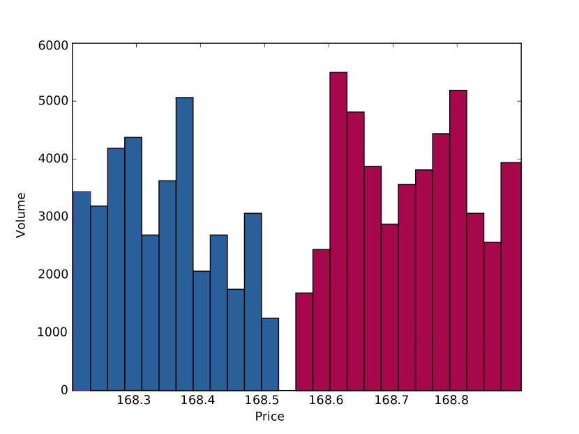
Figure 1: Limit order book at NASDAQ for Apple Inc. (AAPL) on March 29th, 2018.

In an exchange, the traders can primarily submit three different types of orders: limit orders, market orders, and cancellation orders. A limit order is an order to buy or sell a particular number of securities at a specified price or better. A market order is an order to immediately buy or sell a certain number of securities at the best available price in the LOB. The arrival of market orders is instantly executed against the best available price in the limit order book. Orders that exceed the size available at the best price automatically spill over to the next best available price. Unlike market orders, the limit orders rest in the order book, pending execution against a market order or being partially or fully canceled by traders. The limit orders posted near to bid and ask are executed instantly, but may be prolonged if market prices diverge from the requested price. Market makers utilise this attribute to design optimal trading strategies (Spooner et al.,, 2018).

In an exchange, several orders posted by traders can have the same price at a given time $t$. To effectively match the orders within each discrete price level, the LOBs employ various priority mechanism algorithms. The algorithm most commonly employed by various exchanges is price-time. In this case, for buy or sell orders, the matching algorithms give priority to the orders with the highest or lowest price. In the event of ties, preference is given to orders with the earliest submission time relative to other orders (Gould et al.,, 2013). Other prominent priority mechanism algorithms include pro-rata and price-size. Under the pro-rata algorithms, the ties at the given price are broken by distributing orders according to the depth in the LOB, while price-size mechanism algorithms break the ties by giving higher priority to larger orders. Our study makes use of price-time priority mechanism algorithms, as these encourage market makers to submit limit orders when designing their trading strategies.

2.2 High-Frequency Market Making

Market making is a liquidity-providing trading strategy that quotes numerous bids and asks for a security in anticipation of making a profit in the form of bid-ask spread, while maintaining a relatively neutral position (Chakraborty and Kearns,, 2011). The modern market making strategy or high-frequency market making strategy can also be characterized as subset of HFT, where traders uses ”lightning fast with a latency (inter-message time) upper bound of 1 millisecond, only engages in proprietary trading, generates many trades (it participates in 14.4% of all trades, split almost evenly across both markets), and starts and ends most trading days with a zero net position” (Menkveld,, 2013). The foundation of designing optimal market making strategies is dependent on optimising order-handling costs, adversely selected bid or ask quote costs, and non-zero position risk-averse costs(Menkveld,, 2013).

In order to better understand high-frequency market making, let us consider a simple example from LOB illustrated in Figure 1. The market making strategy places a buy order at $100.00$ and sell order at $100.10$. The execution of the both orders will give the traders profit of $00.10$, which is also the spread. As millions of market maker’s trades are executed each second, they can amass huge profits.

However, high-frequency market making strategies are always exposed to the risk of adverse price movements, uncertain executions and adverse selections (Penalva et al.,, 2015). To avoid the above risks, the high-frequency market making strategies seek to compete in the market through lower order-processing costs, fast matching engines and low latency. The fast matching engine reduces the adverse selection risk by facilitating a market-making strategy to immediately update quotes on the arrival order book information, while low latency reduces the search for market venues to mitigate a costly non-zero inventory position (Penalva et al.,, 2015; Menkveld,, 2013). The array of sophisticated statistical or machine learning models used on the real-time order book data serve to optimise the transaction costs, which are directly related to profitability.

2.3 Hawkes Process

To set the stage for Hawkes process, we first explicate key concept related to counting process, point process, and conditional intensity function from the classical literature (Gao et al.,, 2018; Hawkes,, 2018; Bacry et al.,, 2015; Embrechts et al.,, 2011).

Let us consider a positive sequence of event arrival time, $\{t_{n}\}_{n\in\mathbb{N}}$, such that $\forall\ n\in\mathbb{N}$, $t_{n}<t_{n+1}$, defined on probability space $(\Omega,\mathcal{F},\mathbb{P})$ with almost surely finite, right-continuous step function defined for all $t\in\mathbb{R}_{+}$, and complete information filtration $(\mathcal{F}_{t})_{t\geq 0}$, such that $\mathbb{F}=\mathcal{F}^{N}(t)$, $t\geq 0$. Then the counting process $N(t)$ and its analogous point process $L(t)$ is defined as:

$$N(t)=\sum_{n\in\mathbb{N}}\mathbb{I}_{t_{n}\leq t}\quad\text{and}\quad L(t)=\sum_{n\in\mathbb{N}}\ell_{n}\cdot\mathbb{I}_{t_{n}\leq t}$$ (2.1)

where $\mathbb{I}_{\{.\}}$ is the indicator function and $\{\ell_{n}\mathrel{\mathop{\mathchar 58\relax}}n\geq 1\}$ is a sequence of non-negative random variable having independent and identical distribution.

In academic literature, counting and point process terminology is often indistinguishable. The reader is expected to infer the nature of the process depending on the context. For example, point process are often characterized by the distribution function of the occurrence of the event conditioned to the past, but problems associated with the conditional arrival distribution mean that this is not very practical. Instead, the conditional intensity function is used. For counting process $N(t)$ with associated history $\mathcal{H}(t)$ and adapted to a filtration $\mathbb{F}$, we define the conditional intensity as:

$$\lambda(t|\mathbb{F})=\lim_{h\rightarrow 0}\mathbb{E}\bigg{[}\frac{(N(t+h)-N(t))|\mathcal{H}(t)}{h}\bigg{|}\mathbb{F}\bigg{]}$$ (2.2)

We now define Hawkes process characterized by intensity $\lambda(t)$ with respect to its natural filtration as:

$$\lambda(t|\mathbb{F})=\mu(t)+\int_{-\infty}^{t}\phi(t-\tau)\ {dN}(\tau)$$ (2.3)

where $\mu$ is an the baseline intensity and $\phi$ is a non-negative kernel function such that $||\phi||_{1}=\int_{0}^{\infty}\phi(\tau)d\tau<1$. Prominent kernel function used in finance is exponential decay $\phi(t)=\alpha e^{-\beta t}$, where parameter $\alpha$ represents previous event weight and $\beta$ past event duration.

Now, we consider $N(t)=\{N_{t}^{i}\}_{i=1}^{M}$ as the M-dimensional counting process, and its analogous point process as $\{L_{t}^{i}\}_{i=1}^{M}$. Similarly, we define the multidimensional Hawkes process as:

$$\lambda_{i}(t|\mathbb{F})=\mu_{i}+\sum_{j=1}^{M}\int_{0}^{t}\phi_{i,j}(t-\tau)dN_{j}(\tau),$$ (2.4)

where, $\mu=\{\mu_{i}\}_{i=1}^{M}$ a baseline intensity vector and $\phi(t)=\{\phi_{i,j}(t)\}_{i,j=1}^{M}$ a matrix-valued kernel that is component-wise non-negative, causal, and $L^{1}$-integrable (Bacry et al.,, 2015).

We can also enrich the Equation 2.4 by associating each event with time of event $t_{n}$, its component $\varkappa_{n}$ and mark $k_{n}$. For example, modeling the trades performed at event time $t_{n}$ with different volume $k_{n}$ and drawdown intensity $\varkappa_{n}$ (Bacry et al.,, 2015). The vector intensity function of the multivariate marked Hawkes process will be defined as:

$$\lambda_{i}(t,n|\mathbb{F})=\mu_{i}+\sum_{j=1}^{M}\int_{0}^{t}\phi_{i,j}(t-\tau)\psi_{j}(n)dN_{j}(\tau\times\delta),$$ (2.5)

where, $\mu=\{\mu_{i}\}_{i=1}^{M}$ a exogenous intensities vector, $\phi(t)=\{\phi_{i,j}(t)\}_{i,j=1}^{M}$ a matrix-valued kernel and $\psi_{j}(n)$ a impact function of marks.

The properties of the Hawkes process can be characterized thoroughly in an analytical manner due to the linear structure of the stochastic intensity (Hawkes,, 2018; Bacry et al.,, 2015).The linear properties of a Hawkes process enable linear predictions of the models, given their base intensity and the kernels as parameters (the kernels are non-parametrically calibrated from the data). A Hawkes process can be appropriately approximated as auto-regressive process, wiener processes, and clustering representation (Bacry et al.,, 2015). Simply put by Mei and Eisner, (2017), ” the Hawkes process supposes that past events can temporarily raise the probability of future events, assuming that such excitation is positive, additive over the past events, and exponentially decaying with time”. In a simplified setting, these properties might be useful for modelling constrained processes, but might not be applicable to real world examples. For example, at large scales, the price formation process’s microscopic variables, as they relate to order book events, do not diffuse toward Wiener processes. Similarly, the massive cancellation of orders in LOB might inhibit price rather than exciting it.

2.4 Neural Hawkes Process

The Neural Hawkes Process was (NHP) introduced to fill the gaps in the Hawkes process’s unrealistic assumptions. Building on the earlier formulation, the positivity constraints on baseline intensity vector $\mu$, kernels $\phi$, and decay rate $\delta$ limit the eloquentness of Hawkes process. It fails to capture inhibition and inherent inertia effect, which are characteristics of realistic financial market (Mei and Eisner,, 2017).

Let $\{t_{n},\varkappa_{n},k_{n}\}_{n\in\mathbb{N}}$ is a event streams, where $t_{n}$ are times of occurrence of an event, its component $\varkappa_{n}$, and their corresponding mark $\{k_{n}\}_{n\in\mathbb{N}}$ in $k_{n}\mathrel{\mathop{\mathchar 58\relax}}=\{1,\dots,K\}$. Then, the probability of incidence of next event at time $t_{n}$ of type $k_{n}$ is $\mathbb{P}\{(t_{n},\varkappa_{n},k_{n})\mid\mathcal{H}_{n},(t_{n}-t_{n-1})\}dt$. The associated intensity function conditioned on the past events $\overline{h}$ for self-exciting multivariate point process or Hawkes process with exponentially decaying kernel function is:

$$\lambda_{k}(t)=\mu_{k}+\sum_{\overline{h}\mathrel{\mathop{\mathchar 58\relax}}t_{\overline{h}}<T}=\alpha_{k_{\overline{h}},k}\exp(-\beta_{k_{\overline{h}},k}(t-t_{\overline{h}})),$$ (2.6)

The inhibition and inherent inertia effect are introduced in the self-modulating model, where we relax positivity constraints on parameters $\alpha$ and $\mu$. The negative total resultant activation is then passed through non-linear transfer function (e.g. rectified linear unit (ReLU) function, softplus function etc.) such that:

$$\lambda_{k}(t)=f_{k}(\tilde{\lambda}_{k}(t)),$$ (2.7)

$$\tilde{\lambda}_{k}(t)=\mu_{k}+\sum_{\overline{h}\mathrel{\mathop{\mathchar 58\relax}}t_{\overline{h}}<t}\alpha_{k_{\overline{h}},k}\exp(-\beta_{k_{\overline{h}},k}(t-t_{\overline{h}})).$$ (2.8)

where $\mu_{k}<0$, $\alpha_{j,k}<0$ allows inertia and inhibition effect respectively (Mei and Eisner,, 2017).

The summation in Equations 2.8 places a restriction on the $\tilde{\lambda}_{k}(t)$, where past events have an independent and additive influence. This deviates from reality, which is characterised by the existence of complex dependence between the intensities in terms of number of order event types and past event timings (Bacry et al.,, 2015). Mei and Eisner, (2017) proposed the Neural Hawkes Process to learn and predict complex dependency by replacing the summation with a novel recurrent neural network. In this novel process, the hidden state vector $\mathbf{h}(t)$ controls the dynamics of time varying event intensities, which in turn depends on a vector $\mathbf{c}(t)$ of memory cells in a continuous-time long short-term memory (Hochreiter and Schmidhuber,, 1997).

2.5 Long Short-Term Memory

The central idea of LSTM is the use of memory cell, which overcomes the problem associated with vanishing gradient (Arras et al.,, 2019). The memory cell of LSTM is a complex unit, built from alike nodes in a distinct connectivity pattern, with the novel inclusion of multiplicative nodes, represented in figure 2. A typical LSTM memory cell architecture contains a cell input activation vector ${{x}}_{t}$, an input gate ${{i}}_{t}$, a forget gate ${{f}}_{t}$, a cell ${{c}}_{t}$, an output gate ${{o}}_{t}$ and an output response $h_{t}$. The distinctive feature of the LSTM approach, input gate and forget gate, govern the information flow into and out of the cell according to gate logic. Whereas, the output gate controls the amount of information flow from the cell to the output ${{h}}_{t}$. A self-connected recurrent edge with fixed unit weight in the memory cell ensures that error can flow across many time steps without vanishing or exploding.

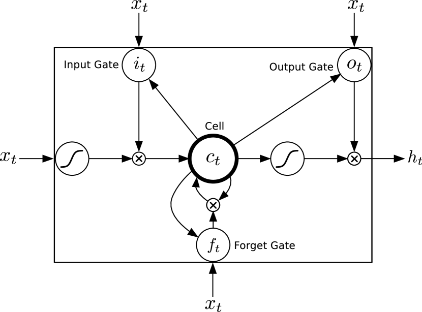
Figure 2: LSTM Memory Cell (Zhu et al.,, 2016).

At each time step $t$, the recursive computation in the LSTM model proceeds according to the following equations:

$$\begin{aligned} \!&{\bf{i}}_{t}=\sigma\left({{\bf{W}}_{xi}}{{\bf{x}}_{t}}+{{\bf{W}}_{hi}}{\bf{h}}_{t-1}+{{\bf{W}}_{ci}}{\bf{c}}_{t-1}+{\bf{b}}_{i}\right),\\ \!&{\bf{f}}_{t}=\sigma\left({{\bf{W}}_{xf}}{{\bf{x}}_{t}}+{{\bf{W}}_{hf}}{\bf{h}}_{t-1}+{{\bf{W}}_{cf}}{\bf{c}}_{t-1}+{\bf{b}}_{f}\right),\\ \!&{\bf{\overline{c}}}_{t}=\phi\left({{\bf{W}}_{xc}}{{\bf{x}}_{t}}\!+\!{{\bf{W}}_{hc}}{\bf{h}}_{t-1}\!+\!{\bf{b}}_{c}\right),\\ \!&{\bf{c}}_{t}={\bf{f}}_{t}\!\odot{\bf{c}}_{t-1}\!+{\bf{i}}_{t}\!\odot{\bf{\overline{c}}}_{t},\\ \!&{\bf{o}}_{t}=\sigma\left({{\bf{W}}_{xo}}{{\bf{x}}_{t}}+{{\bf{W}}_{ho}}{\bf{h}}_{t-1}+{{\bf{W}}_{co}}{\bf{c}}_{t}+{\bf{b}}_{o}\right),\\ \!&{\bf{h}}_{t}={\bf{o}}_{t}\odot\phi\left({\bf{c}}_{t}\right),\end{aligned}$$ (2.9)

where ${{x}}_{t}$ is input vector at time $t$, the activation function $\sigma\left(x\right)$ / $\phi\left(x\right)$ is defined as sigmoid $\sigma\left(x\right)=1/(1+e^{-x})$ / $\phi\left(x\right)=\tanh$, ${\bf{W}}_{AB}$ is the weight matrix between $A$ and $B$ (e.g., ${\bf{W}}_{xi}$ is the weight matrix from the inputs ${\bf{x}}_{t}$ to the input gates ${\bf{i}}_{t}$), ${\bf{b}}_{B}$ denotes the bias term of $B$ with $B\in\{i,f,c,o\}$ and $\odot$ denotes point-wise multiplication of the two vectors. To ensure comprehensibility with standard literature, we follow the same naming conventions discussed in the paper by Zhu et al., (2016).

3 Literature Review

In this section, we briefly review three prominent streams of research into how the Hawkes process is used to design market making strategies. We are well aware of blurred and overlapping boundaries across research streams, but strongly believe in capturing the essence of Hawkes models in market making.

3.1 Stochastic Optimal Control

The classical finance literature employs a stochastic optimal control framework to determine market maker’s optimal quotes for bid and ask in the presence of inventory risk, adverse selection, information asymmetry and latency (Ho and Stoll,, 1981; Sandas,, 2001; Avellaneda and Stoikov,, 2008; Penalva et al.,, 2015). The market maker aims to maximise the expected utility of the profit and loss contour at closing time. By integrating a utility framework into the microstructure of LOB, Avellaneda and Stoikov, (2008) were able to analytically derive optimal bid and ask quotes. In the continuous-time model, the mid-prices evolve according to Brownian motion, and the order arrival follows a Poisson process. In one particular case, a non-homogeneous Poisson process is reduced to the Hawkes process (Bacry et al.,, 2015). The unrealistic assumptions limit the model’s ability to capture adverse selection effects, market impact and autocorrelation structures in the security being traded. Building on the seminal work off Avellaneda and Stoikov, (2008), numerous researchers looked at price impact, adverse selection effects, and latency, together with different objective functions (Penalva et al.,, 2015). The purpose of all of the improvements in the model is to provide numerical approximations for the associated stochastic differential equations. However, problems related to model ambiguity have yet to be addressed (Nystrom et al.,, 2014).

The profusion of transaction-level data at a minuscule resolution provides an unprecedented opportunity to apply Hawkes processes to the study of market microstructure with a view to deciphering price formation mechanism, liquidity dynamics and volatility (Morariu-Patrichi and Pakkanen,, 2018). The use of Hawkes processes to model extreme price moves and order flow is well integrated with the high- frequency market making model (Nystrom et al.,, 2014; Bacry et al.,, 2015). For example, Nystrom et al., (2014) proposed a market making model based on model risk or uncertainty, in which inventory dynamics, fill rates and price formation are modelled using two independent Hawkes processes. While the market making models based on the Hawkes processes have been moderately successful in integrating a realistic order arrival process, they fail to incorporate the complex interaction between the self- and cross-excitation effects of the endogenous state variables that describe the LOB (Morariu-Patrichi and Pakkanen,, 2018). In the classical ”buy low and sell high” market making strategies, (Cartea et al.,, 2014) used a multivariate Hawkes process to capture the interaction between market orders and the state of LOB. However, the constraints placed on parametric specification for conditional intensity by the Hawkes process limit the model’s eloquence.

3.2 Agent-Based Models

Market making has been also been extensively investigated in ABM (Das,, 2005; Wah et al.,, 2017). Using a bottom-up approach, the ABMs try to artificially simulate the systems’ aggregate behaviours caused by the actions and interactions between heterogeneous autonomous agents (Samanidou et al.,, 2007). The ABMs in market making range from the simple ”zero intelligence” of mainstream economics to representing in detail the full complexity of the order book and market microstructure. The seminal work of Muni Toke, (2011) assimilated a microscopic, dynamical statistical model for the continuous double auction (Smith et al.,, 2003) into Hawkes framework. The reinforced zero-intelligence market making model populated with the liquidity provider and liquidity taker uses mutually exciting Hawkes processes for the order arrival process. However, the parametric specification of the exponential kernels contradicts the empirical results on the existence of a feedback loop between order arrival and the state of LOB (Gonzalez and Schervish,, 2017; Morariu-Patrichi and Pakkanen,, 2018). The Neural Hawkes process Mei and Eisner, (2017) applied a Neural Hawkes process to natural language processing in order to tackle the parametric specifications problem, and generalised the Hawkes process by calculating the event intensities from the hidden state of an LSTM.

Another prominent ABM in market making research (Wah et al.,, 2017)uses empirical game-theory analysis to examine the effect of market making on market performance in different scenarios. In the paper, the authors use multiple background traders (e.g. traditional zero intelligence agents) to produce realistic market microstructure. The Bayesian market makers were then used to investigate welfare effect, trading gains and strategic behaviour. The simplistic adaptive trading strategies adopted by the market makers ought to be sufficient to investigate market equilibria, but would face serious challenges in relation to developing realistic market making strategies that also take account of market microstructure. The academic literature needs to assimilate the success of artificial intelligence in designing trading strategies that interact with close-to-reality market simulations.

3.3 Artificial Intelligence

The success of deep reinforcement learning in board games (Silver et al.,, 2017) and video games (Mnih et al.,, 2015) soon sent ripples through the world of finance. Drawing on the classical mathematical setup by Avellaneda and Stoikov, (2008), Gueant and Manziuk, (2019) used a model-based deep actor-critic algorithm to find the optimal bid and ask quotes across a high-dimensional space of corporate bonds. Spooner et al., (2018) rreconstructed a limit order book from historical data and used it to construct a market making agent using temporal-difference reinforcement learning. The next natural progression, a multi-agent simulation of a dealer market, was developed by Ganesh et al., (2019) to understand the behaviour of market making agents. The success of this model is dependent on a realistic simulation framework of the financial market. However, algorithmic trading research is evolving, and is still at the stage of exploiting market simulators that could be used to develop training and testing algorithms in a similar vein to the classic Atari 2600 games simulator (Mnih et al.,, 2015).

Despite the exemplary predictive performance of deep learning models, market making has not yet been comprehensively addressed. If we return to stochastic optimal control in market making, we notice that the dynamics of order flow are mostly described by variants of Hawkes processes, while the resultant control algorithms are associated with continuous semi-martingales, which are hard to solve recursively (Gueant and Manziuk,, 2019). In addition, the unavailability of a realistic simulation framework and high-quality order-level data restricts researchers’ ability to replicate the successes of deep learning in market making.

Nevertheless, deep learning models (based on CNN architecture) have done moderately well when it comes to modelling price-formation mechanisms using order book events as input (Sirignano,, 2019; Cont and Sirignano,, 2019; Tashiro et al.,, 2019; Tsantekidis et al.,, 2017). The literature is proof that empirical investigation of order-level data has always augmented the model of choice. In short, the ABM, statistical modelling and artificial intelligence approaches to market making all have desirable attributes that the others lack. For example, the CNN architectures lacks self- and cross-excitation effects while modelling LOB dynamics (Zhang et al.,, 2019). The DLSTM architecture performs hierarchical processing of complex order book events, and as such is able to efficiently capture the temporal structures of LOB (Sagheer and Kotb, 2019a, ; Sagheer and Kotb, 2019b, ). As market making involves placing optimal bids and asks, the DLSTM architecture, together with the Hawkes process, would efficiently model order arrival and price-formation mechanisms by constructing a self-exciting multivariate Hawkes process with limit order state process, which are coupled and interact with each other.

4 Deep Hawkes Process

In this section, we propose that the Deep Hawkes Process (DHP) be used to concurrently model the order book event timings and associated event types. By assimilating it into the order arrival process, the market makers have control over the sending of different orders at specific points in time. The basic idea behind our approach is to view the conditional intensity of the Hawkes process as a nonlinear deterministic function of past history, and to use DLSTM to automatically learn a high-dimensional representation from the data. We believe that capturing the constraints of the Hawkes process and recurrent network architecture enables a replication of the success of the natural language process (Du et al.,, 2016; Mei and Eisner,, 2017) and time series prediction (Sagheer and Kotb, 2019a, ; Sagheer and Kotb, 2019b, ) in market making.

4.1 Deep Long Short-Term Memory

Despite the success of recurrent marked temporal point processes and the Neural Hawkes process across disciplines, the conventional shallow recurrent network architecture and its variant long short-term memory (LSTM) might be inadequate when it comes to modelling noisy asynchronous order book events. Lately, the DLSTM architecture (Sagheer and Kotb, 2019a, ; Sagheer and Kotb, 2019b, ; Zhu et al.,, 2016) used in action modelling and multivariate time series forecasting validated its precedence over traditional LSTM architecture. The architecture of the DLSTM is same as the previously introduced LSTM, apart from the fact that it involves multiple LSTM layers stacked on top of each other.

4.2 DLSTM-SDAE

In an ideal setting, the performance of the DLSTM model proved to be empirically better than existing contemporary statistical and deep modules. However, as the non-linear variables are modelled in such a way as to be scaled up, the overall learning of the models suffers greatly due to the back-propagation algorithm trapped within multiple local minima (Sagheer and Kotb, 2019b, ). This may be the biggest hurdle when it comes to modelling limit order book events that comprise complex, asynchronous non-linear multivariate time series. The ultra-noisy order book data also makes processing more challenging. To circumvent the limitations of the conventional stacked LSTM model, we use the stacked denoising auto-encoder (SDAE) together with DLSTM. The SDAE enables the deep neural networks with multiple nonlinear hidden layers to learn complex features from noisy limit order book data (Li et al.,, 2019; Vincent et al.,, 2010) and resolves the random weight initialization of LSTM’s units problem in DLSTM (Sagheer and Kotb, 2019b, ). Figure 3 shows the proposed DLSTM- based SDAE architecture for DHP.

Figure 3: The DLSTM-SDAE architecture.

As shown in Figure 3, the reconstructed order book data is denoised by SDAEs layers in in DLSTM-SDAE architecture. In this method, at the first layer the input $\bf{x_{t}}$ is corrupted into $\bf{\tilde{x_{t}}}$ using stochastic mapping $\bf{\tilde{x_{t}}}\sim\mathcal{S_{\mathcal{D}}}(\bf{\tilde{x_{t}}}\mid\bf{x_{t}})$. Then, the autoencoder maps corrupted input $\bf{\tilde{x_{t}}}$ to a hidden representation $\mathit{h}=f_{\theta}(\bf{\tilde{x_{t}}})$ with encoder $f_{\theta}(\bf{\tilde{x_{t}}})=(W\bf{\tilde{x_{t}}}+b)$. Lastly, the decoder $g_{\theta^{{}^{\prime}}}$ reconstruct $\bf{z}=g_{\theta^{{}^{\prime}}}(\bf{\tilde{x_{t}}})$ from the hidden representation $\mathit{h}$. The parameters $\theta$ and $\theta^{{}^{\prime}}$ are trained using stochastic gradient descent to minimize reconstruction error measured in the squared error loss $L_{2}(\bf{x},\bf{z})=\mathinner{\!\left\lVert\bf{x}-\bf{z}\right\rVert}^{2}$. Once mapping is learned, the high-level hidden state $\mathit{h}$ is applied for training the next layer. For detail learning procedure in SDAE, please refer to seminal paper on the subject (Vincent et al.,, 2010).

At time $t$, the denoised input $\bf{x_{t}}$ from SDAE is then passed to first layer of LSTM together with previous hidden state $h^{1}_{t-1}$. The hidden state at time $t$, $h^{1}_{t}$ is calculated using recursive LSTM procedure discussed in Equation 2.9. Its is then moved to next time step and LSTM layers. In the second layer, the hidden state $h^{1}_{t}$ and the previous $h^{2}_{t-1}$ is used to compute $h^{2}_{t}$ and procedure repeats until last layer is complied.

4.3 Model Formulation

Let $\{t_{n},\varkappa_{n},k_{n}\}_{n\in\mathbb{N}}$ be a stream of order book event, where $t_{n}$ are times of occurrence of an event, its component $\varkappa_{n}$, and their corresponding mark $\{k_{n}\}_{n\in\mathbb{N}}$ in $k_{n}\mathrel{\mathop{\mathchar 58\relax}}=\{1,\dots,K\}$. Then, the probability that the next event occurs at time $t_{n}$ is of type $k_{n}$ is $\mathbb{P}\{(t_{n},\varkappa_{n},k_{n})\mid\mathcal{H}_{n},(t_{n}-t_{n-1})\}dt$. We are interested in the model to predict next event stream $\{t_{n},\varkappa_{n},k_{n}\}$ given a past history of event $k_{n}$, evaluate its likelihood and simulate the next event stream by learning from the past event stream. Equation 4.1 shows the associated intensity function of the DHP with relaxed positivity constraints:

$$\lambda_{k}(t)=f_{k}(\bf{w}_{k}^{\top}\bf{h}(t))$$ (4.1)

The hidden state $\bf{h}(t)$ is updated from the memory sell $\bf{c}(t)$ as in Equation 4.2.

$$\bf{h}(t)=\bf{o}_{n}\odot\phi(\bf{c}(t))\text{ for }t\in(t_{n-1},t_{n}]$$ (4.2)

The life of interval $(t_{n-1},t_{n}]$ is determined by the next event $k_{n}$ at $t_{n}$, DLSTM reads $\{t_{n},\varkappa_{n},k_{n}\}$ and updates the current memory cells $\bf{c}(t)$ to $\bf{c}_{n+1}$, associated with hidden state $\bf{h}(t_{n})$. The other parameters of the DLSTM are recursively updated according to the Equation 4.3.

$$\begin{aligned} \!&{\bf{i}}_{n+1}=\sigma\left({{\bf{W}}_{xi}}{{\bf{x}}_{n}}+{{\bf{W}}_{hi}}{\bf{h}}(t_{n})+{{\bf{W}}_{ci}}{\bf{c}}(t_{n})+{\bf{b}}_{i}\right),\\ \!&{\bf{f}}_{n+1}=\sigma\left({{\bf{W}}_{xf}}{{\bf{x}}_{n}}+{{\bf{W}}_{hf}}{\bf{h}}(t_{n})+{{\bf{W}}_{cf}}{\bf{c}}(t_{n})+{\bf{b}}_{f}\right),\\ \!&{\bf{\overline{c}}}_{n+1}=\phi\left({{\bf{W}}_{xc}}{{\bf{x}}_{n}}\!+\!{{\bf{W}}_{hc}}{\bf{h}}(t_{n})\!+\!{\bf{b}}_{c}\right),\\ \!&{\bf{c}}_{n+1}={\bf{f}}_{n+1}\!\odot{\bf{c}}(t_{n})\!+{\bf{i}}_{n+1}\!\odot{\bf{\overline{c}}}_{n+1},\\ \!&{\bf{\widehat{c}}}_{n+1}={\bf{\widehat{f}}}_{n+1}\!\odot{\bf{\widehat{c}}}(t_{n})\!+{\bf{\widehat{i}}}_{n+1}\!\odot{\bf{\overline{c}}}_{n+1},\\ \!&{\bf{o}}_{n+1}=\sigma\left({{\bf{W}}_{xo}}{{\bf{x}}_{n}}+{{\bf{W}}_{ho}}{\bf{h}}(t_{n})+{{\bf{W}}_{co}}{\bf{c}}(t_{n})+{\bf{b}}_{o}\right),\\ \!&{\bf{\bar{\bar{s}}}}_{n+1}=f\left({{\bf{W}}_{xd}}{{\bf{x}}_{n}}+{{\bf{W}}_{hd}}{\bf{h}}(t_{n})+{{\bf{W}}_{cd}}{\bf{c}}(t_{n})+{\bf{b}}_{d}\right),\end{aligned}$$ (4.3)

where $\bf{x}_{n}$ is $n^{th}$ input vector represented by one hot encoding of new order book event $k_{n}$; the activation functions $\sigma\left(x\right)$ / $\phi\left(x\right)$ are sigmoid / hyperbolic tangent function, respectively; ${\bf{W}}_{AB}$ (e.g., ${\bf{W}}_{ci}$) is the weight matrix from the memory cell to input gate vector; ${\bf{b}}_{B}$ denotes the bias term of $B$ with $B\in\{i,f,c,o,d\}$, $\bf{\bar{\bar{s}}}$ is exponential decay parameter and $f(x)=s\log(1+\exp(x/s))$, $s>0$ is scaled soft plus function. As it can be seen in the Equation 4.3, the parameters are updated using the hidden state $\bf{h}(t_{n})$ at time $t_{n}$, succeeding its decay over interval $t_{n}-t_{n-1}$ rather previous hidden state (Equation 2.9). The memory cell ${\bf{c}}(t)$ on the interval $(t_{n-1},t_{n}]$ follows power-law distribution decaying from ${\bf{c}}_{n+1}$ to ${\bf{\widehat{c}}}_{n+1}$ and defined as:

$$\bf{c}(t)={\bf{\widehat{c}}}_{n+1}+\left({\bf{c}}_{n+1}-{\bf{\widehat{c}}}_{n+1}\right)\left(\left(t-t_{n}\right)^{{-\bf{\bar{\bar{p}}}}_{n+1}}\right)\text{ for }t\in(t_{n},t_{n+1}]$$ (4.4)

The DHP, with novel discrete update of stacked LSTM state, allows the model to capture a delayed response, fits non-interacting event pairs, and copes with partially observed event streams. Mei and Eisner, (2017) discuss in detail these benefits of the neural version of the model. In order to ensure mathematical tractability, we have illustrated parameter updates for one of the layers of stacked LSTM, but this can be easily extended to deep architecture. For example, the hidden state ${\bf{h}}^{b}$ at block $b$ in stacked LSTM is recursively computed from $b=1\,\text{:}\,N$ and $t=1\,\text{:}\,T$ using ${\bf{h}}^{b}_{t}=\sigma({{\bf{W}}_{h^{b-1}h^{b}}}{\bf{h}}^{b-1}_{t}+{{\bf{W}}_{h^{b}h^{b}}}{\bf{h}}^{b}_{t-1}+{\bf{b}}_{h})$.

4.4 Feedback Loop Exploration

The empirical results (Morariu-Patrichi and Pakkanen,, 2018; Gonzalez and Schervish,, 2017) indicate the existence of feedback loop between the order flow and the shape of the LOB, together with the self- and cross-excitation effects. In order to efficiently capture this feedback effect in high-dimensional parameter space, we infuse the feedback loop exploration process into the DLSTM-SDAE architecture, as discussed in Figure 3. In connection with designing the deep network architecture and appropriate regularisation, we take into consideration that the network can automatically explore distinct feedback loops for different types of events and their codependency. For example, the feedback effect of market buy and sell orders on price, volume and the bid-ask spread of LOB.

Consequently, we design a fully connected deep network in which each neuron represents an LOB state or feedback effect of the preceding layer, in order to automatically explore the feedback loop. Furthermore, the neurons in the same layer are partitioned into $\mathfrak{B}$ blocks to take into account different combinations of feedback loops. The corresponding regularisation is incorporated into the loss function and described by:

$$\!\mathfrak{L}\!=\!\min_{{\bf{W}}_{xB}}{\mathfrak{L}}\!+{\lambda}_{1}\!\!\sum_{\begin{subarray}{c}B\in S\end{subarray}}{\left\|{\bf{W}}_{xB}\right\|}_{1}\!\!+\!{\lambda}_{2}\!\sum_{\begin{subarray}{c}B\in S\end{subarray}}\sum_{{\mathfrak{b}}=1}^{\mathfrak{B}}\left\|{{\bf{W}}_{xB,{\mathfrak{b}}}}^{T}\right\|_{2,1}\!,$$ (4.5)

where $\mathfrak{L}$ is the loss function of the DLSTM, and other two terms are feedback loop regularization applied to each block in the network (Zhu et al.,, 2016). ${\bf{W}}_{xB}\!\in{\mathbb{R}}^{N_{N}\times K_{J}}$ is weight matrix, with number of neurons $N_{N}$ and inputs dimension $K_{J}$. The $S$ characterizes the set of gates and cell in LSTM neurons for each block in DLSTM. Lastly, the $\left\|{\bf{W}}\right\|_{2,1}\!\!=\!\!\sum_{i}\!\!\sqrt{\sum_{j}\!\!w_{i,j}^{2}}$ is a structural $\ell_{21}$ norm. The loss function (Equation 4.5) was solved by using Adaptive Moment Estimation (Adam) (Kingma and Ba,, 2015). Adam optimization is an augmentation to stochastic gradient descent that is memory efficient, extremely insensitive to hyperparameters, works with sparse gradients, is appropriate for non-stationary objectives, and learns the learning rates itself on a per-parameter basis. It is well suited for highly noisy and/or sparse-gradient order book data.

4.5 Parameters Estimation

Given a collection of sequence of order book events $\mathcal{S}$, $\{t_{n},\varkappa_{n},k_{n}\}_{n\in\mathbb{N}}$, the the log-likelihood of the model can be expressed as the sum of the log-intensities of lapsed event minus an integral of the aggregate intensities over the whole interval observed till $T$:

$$\mathcal{L}\!=\!\ \sum_{n\mathrel{\mathop{\mathchar 58\relax}}t_{n}\leq T}\!\!\log\lambda_{k_{n}}(t_{n})\!-\int_{t=0}^{T}\!\!\lambda(t)dt,$$ (4.6)

The parameter $(k,t)$ is estimated maximizing $\mathcal{L}$ using Adam (Kingma and Ba,, 2015) and Monte Carlo methods (Mei and Eisner,, 2017). The frequently used thinning algorithm adapted from multivariate Hawkes process is then used to sample random sequence from the model.

5 Multi-Agent Simulation Framework

Multi-agent-based modelling is a bottom-up computational modelling approach intended to artificially simulate the aggregate behaviours of systems caused by the actions and interactions between heterogeneous autonomous agents in an environment or environments (Samanidou et al.,, 2007). In this section, we describe the important components of multi-agent-based modelling, including environment (market simulator), agent ecology (trading strategies) and reward (profit and loss), to study the behaviour of market making agents whose strategies employ Deep Hawkes processes.

5.1 Market Simulator

The market simulator is an essential tool for designing, evaluating and backtesting algorithmic trading strategies under various market scenarios. The market is flooded with various proprietary and open- source financial simulation frameworks, but the constraints associated with licences, application interfaces and software design limit their usability (Maeda et al.,, 2020; Izumi and Toriumi,, 2009). In this paper, we have designed a multi-asset market simulator from scratch, which is scalable to markets of substantial size. The asynchronous event-based interface is built over realistic market architecture, interface kernels, a matching engine and the Financial Information eXchange (FIX) protocol – an open electronic communications protocol standard used to carry out trades in electronic exchanges.

5.1.1 Market Architecture

The market architecture consolidates the communication interface, market and matching engine. Figure 4 outlines key components of market architecture and their interaction from a high-level perspective. The agents connect to the market via a kernel that hosts order management details. This acts as a transmission channel between agents and markets, thereby providing the extreme throughput and lowest latency for order transactions. It also throttles the amount of transactions, as per the market requirement. As such, there is a guarantee of fairness between agents waiting to place orders. The markets represent an information interchange, in which heterogeneous agents communicate through kernels for order transactions, processing and execution according to the matching engine, as per the financial instruments. The markets respond to order status by sending an execution report that covers the period from start to market reset event. This provides opportunities for agents to tweak the parameters in their trading strategies after every trading period if required.

Figure 4: Market Simulator.

5.1.2 Communication Interface

The communication interface between agents and markets follows the FIX standard protocol to increase efficiency, competition and innovation. It is an electronic communications protocol designed for the real-time exchange of information between agents and exchanges, including agent identifiers, order identifiers, order handling, trade notifications, broadcasts and execution reports. The widespread adoption of the FIX protocol across financial markets reduces costs associated with connectivity, regulatory compliance, liquidity searches and transactions. Using the FIX protocol, multiple agents can interact with the market via kernels, simultaneously and independently.

5.1.3 Matching Engine

At the core of the market simulator are several matching engines for different financial instruments. Each matching engines matches bids and asks to execute trades in specific instruments. The orders are matched using price-time priority mechanisms. In this context, among bids or asks, the matching algorithms give priority to orders with the highest or lowest price. The ties are broken by giving preference to orders with the earliest submission time compared to other orders. Other well-known priority mechanism algorithms are pro-rata and price-size (Gould et al.,, 2013).

5.2 Market Ecology

The success of a financial simulation framework depends on the precise representation of market ecology that can adequately mimic the real market design. In finance literature, the term ”market ecology” (Farmer,, 2002) refers to the composition of heterogeneous trading strategies that keep evolving over time in response to pressure from a contrasting market. The correct mapping of financial market ecology requires the availability of agent-resolved order-level data, which enables identification of sources and events in the market. In the absence of agent-resolved data, the trading strategies are classified by theoretical considerations, the results of surveys, direct investigations of the trading profile of classes of investors and proxies for HFT (Kirilenko et al.,, 2017; Mankad and Michailidis,, 2013). In this paper, we adapt the market ecology from the different strands of academic literature (McGroarty et al.,, 2019; Paulin et al.,, 2019; Musciotto et al.,, 2018; Kirilenko et al.,, 2017; Leal et al.,, 2016; Mankad and Michailidis,, 2013; Toth et al.,, 2012).

5.2.1 Deep Hawkes Market Makers

Despite the existence of sophisticated market making strategies, the classical ”buy low and sell high” strategy (Cartea et al.,, 2014) is a preferred strategy to make money in the securities market. The success of making a profit from short-term price predictions on bids and asks hinges on placing orders at precisely the right time. The mathematical modelling of the complicated order arrival process is done using the Poisson process (Chakraborti et al.,, 2011), which assumes that orders arrive randomly. However, this is contrary to empirical findings, which show that order arrival times are strongly connected (Rambaldi et al.,, 2017), have self- and cross-excitation effects (Morariu-Patrichi and Pakkanen,, 2018) and that a feedback loop exists between the order arrival and the state of the LOB (Gonzalez and Schervish,, 2017). In this article, we incorporate the feedback loop between order arrival and the state of the limit order book, together with self- and cross- excitation effects, using DHP, to design a high-frequency market making strategy.

The order book events in the securities market are stochastically excited or impeded by a pattern in the past event streams. The market makers are interested in learning the distribution and structure of order book events stream to accurately predict the next order (limit orders, market orders, cancellations, etc.) together with an associated labels (price, volume, etc.). Given a stream of order book events $\{t_{n},\varkappa_{n},k_{n}\}_{n\in\mathbb{N}}$, the market makers calculate the probability that the next event occurs at time $t_{n}$ is of type $k_{n}$ and its probability density conditioned on the history of events $\mathcal{H}_{n}$ by:

$$\lambda(t)dt=\mathbb{P}\{(t_{n},\varkappa_{n},k_{n})\mid\mathcal{H}_{n},(t_{n}-t_{n-1})\}.$$ (5.1)

$$f_{n}(t)=\lambda(t)\exp\left(-\int_{t_{n-1}}^{t}\lambda(\tau)d\tau\right).$$ (5.2)

To predict the time and the next event having minimum loss without information about the time $t_{n}$, we choose $\hat{t}_{n}=\int_{t_{n-1}}^{\infty}tf_{n}(t)dt$ and $\hat{k}_{n}=\operatorname*{arg\,max}_{k}\int_{t_{n-1}}^{\infty}\frac{\lambda_{k}(t)}{\lambda(t)}f_{n}(t)dt$. The associated intensity function for calculating the next order book events is the same as DHP as described in Equation 4.1.

The real securities market has numerous distinct order book events, which is difficult to incorporate in our simulation framework. For the sake of computational tractability, we decided to only include limit order buy/sell, market order buy/sell, and partial/full cancellations. We also assume that the high-frequency market maker is trading a single security in a market whose price at time $t$ is denoted by $p_{t}$. Unlike traditional market making strategies (Spooner et al.,, 2018), the DHP market makers can trade with rational limit or market order quantity, price surge and bid-ask spread distributions.

The deep hawkes market maker (DHMM) place orders at a specified depth relative to the mid-price, $\overline{p_{t}}$. At each time step $t$, the DHMM agent’s pricing mechanism is given by:

$$p^{a,b}_{t}=\overline{p_{t}}+\sum_{i=1}^{\overline{\delta}}i\cdot\mathbf{J}^{i,u}_{t}-\sum_{i=1}^{\overline{\delta}}i\cdot\mathbf{J}^{i,d}_{t}$$ (5.3)

where $\overline{p_{t}}$ is the mid price at time $t$, $\mathbf{J}^{i,u}$ is the number of upward jumps with $i$ ticks, and $\mathbf{J}^{i,d}$ is the number of downward jumps with $i$ ticks between $0$ and $t$, $i=1,\dotsc,\overline{\delta}$. The intensities of $\mathbf{J}^{i,u}$ and $\mathbf{J}^{i,d}$ are $\lambda_{k,u}(t)$ and $\lambda_{k,d}(t)$, respectively,

$$\lambda_{k,i}(t)=f_{k,i}(\bf{w}_{k,i}^{\top}\bf{h}(t)),\;\;k=u,d.$$ (5.4)

The parameters of the Equation 5.4 are calculated as discussed under model formulation in Section 4.3.

Most of the quantitative finance research into the high-frequency market making problem is based on the assumption of constant order size (Huang et al.,, 2015). However, the empirical analyses suggests that the order sizes have striking statistical distribution at different timescales (Lu and Abergel,, 2018; Rambaldi et al.,, 2017; Mu et al.,, 2009). The limit order size follows $\mathfrak{q}$-Gamma distribution (Mu et al.,, 2009). The market maker’s willingness to sell or buy specified quantities of securities is defined as:

$$q^{a,b}_{lt}=\left[\Gamma(\alpha,\beta)\right]^{q_{max}}_{q_{min}}\cdot\left(\frac{I_{t}\pm\bar{I}}{\bar{I}}\right),$$ (5.5)

where $I_{t}$ is inventory at time $t$, $\bar{I}$ maximum inventory, and $\Gamma(\alpha,\beta)$ is $\mathfrak{q}$-Gamma distribution is described as:

$$\Gamma(\alpha,\beta;q)=\frac{1}{Z}\left(\frac{q}{\alpha}\right)^{\beta}\left[1-(1-\mathfrak{q}){\frac{q}{\alpha}}\right]^{\frac{1}{1-\mathfrak{q}}}~{},$$

$$Z=\int_{0}^{\infty}\left(\frac{q}{\alpha}\right)^{\beta}\left[1-(1-\mathfrak{q}){\frac{q}{\alpha}}\right]^{\frac{1}{1-\mathfrak{q}}}{\rm{d}}q.$$

One striking feature of equity markets is the existence of short- lived limit orders that are modified or cancelled once every 50 milliseconds (Dahlström et al.,, 2018). The limit order cancellation is an important characteristic of market making strategies that are related to expected profit, bid-ask spread and order queue position. We model cancellation sizes as follows:

$$q^{a,b}_{ct}=\left[P_{c}(q;Q)\right]^{q_{max}}_{q_{min}}\cdot\left(\frac{I_{t}\pm\bar{I}}{\bar{I}}\right),$$ (5.6)

where $P_{c}(q;Q)$ is truncated geometric distribution (Lu and Abergel,, 2018). The LOB is represented as $[Q_{-i}\mathrel{\mathop{\mathchar 58\relax}}i=1,\ldots,L]$ and $[Q_{i}\mathrel{\mathop{\mathchar 58\relax}}i=1,\ldots,L]$ with corresponding quantities $q_{i}$. The truncated geometric distribution is defined as:

$$P_{c}(q;Q)=\mathbb{P}[q|Q]=\frac{p_{c}^{0}(1-p^{0}_{c})^{q-1}}{1-(1-p^{0}_{c})^{Q}}\mathbbm{1}_{\{q\leq Q\}}.$$

Finally, the market order follows a mixture of truncated geometric distribution and the dirac delta distribution (Lu and Abergel,, 2018). The market order size that a market maker is willing to buy or sell is described as:

$$q^{a,b}_{mt}=\left[P_{m}(q;Q)\right]^{q_{max}}_{q_{min}}\cdot\left(\frac{I_{t}\pm\bar{I}}{\bar{I}}\right),$$ (5.7)

$$P_{m}(q;Q) =\theta_{0}\frac{p_{m}^{0}(1-p_{m}^{0})^{q-1}}{1-(1-p_{m}^{0})^{Q}}\mathbbm{1}_{\{q\leq Q\}}$$

$$+\sum_{k=1}^{\lfloor\frac{Q-1}{5}\rfloor}\theta_{k}\mathbbm{1}_{\{q=5k+1\}}+\theta_{\infty}\mathbbm{1}_{\{q=Q,Q\neq 5n+1\}}.$$

The parameters $\{p_{c}^{0},p_{m}^{0},\theta_{0},\theta_{k},\theta_{\infty}\}$ are estimated using a maximum likelihood method. The details of estimation and calibration can be retrieved from the Lu and Abergel, (2018). The market orders are used to clear the unexecuted inventory at the end of trading.

5.2.2 Probabilistic Market Makers

To ensure fair competition with DHMM and incorporate the existing state-of-the-art, we include a probabilistic estimate-based benchmark strategy (Das,, 2005) adapted to our simulation framework. In this market making strategy, the agent attempts to track the fundamental price of securities by maintaining a probability density estimate of the fundamental price.

The probabilistic market makers (PMM) intent to sell or buy $q$ unit of security at time $t$ for price $p^{a,b}_{t}$ in a market populated with uninformed, informed and noisy informed agents. Let us assume that the fundamental price of the security at time $t$ is $f_{t}$, $\xi$ be the fraction of informed agents and the probability of buy or sell orders by the uninformed agents is $\zeta$. The noisy informed agents assumes that the price of securities follow normal distribution $p_{t}\;=\;f_{t}+\mathcal{N}_{s}(0,\sigma^{2}_{n})$. Whereas the fundamental price of security evolves according to a jump process. The order book event defines the jump and prices follow normal distribution. The PMM ask and bid prices at time $t$ are then defined as:

$$\begin{split}p^{a,b}_{t}&=\frac{1}{P_{Buy,Sell}}\sum_{f_{t}=f_{min}}^{f_{t}=p^{a,b}_{t}}\left[\left((1-\xi)\zeta+\mathsf{Pr}(\mathcal{N}_{s}(0,\sigma^{2}_{n})\gtrless(p^{a,b}_{t}-f_{t}))\right)f_{t}\mathsf{Pr}(f=f_{t})\right]\\ &+\frac{1}{P_{Buy,Sell}}\sum_{f_{t}=p_{t}^{a,b}+1}^{f_{t}=f_{max}}\left[\left((1-\xi)\zeta+\mathsf{Pr}(\mathcal{N}_{s}(0,\sigma^{2}_{n})\lessgtr(f_{t}-p^{a,b}_{t}))\right)f_{t}\mathsf{Pr}(f=f_{t})\right]\end{split}$$ (5.8)

$$\begin{split}P_{Buy,Sell}&=\sum_{f_{t}=f_{min}}^{f_{t}=p^{a,b}_{t}}\left[(1-\xi)\zeta+\mathsf{Pr}(\mathcal{N}_{s}(0,\sigma^{2}_{n})\gtrless(p^{a,b}_{t}-f_{t}))\right]\mathsf{Pr}(f=f_{t})\\ &+\sum_{f_{t}=p_{t}^{a,b}+1}^{f_{t}=f_{max}}\left[(1-\xi)\zeta+\mathsf{Pr}(\mathcal{N}_{s}(0,\sigma^{2}_{n})\lessgtr(f_{t}-p^{a,b}_{t}))\right]\mathsf{Pr}(f=f_{t})\end{split}$$

where $P_{Buy,Sell}$ is a priori probability of a buy or sell order and $\mathcal{N}_{s}(0,\sigma_{n})$ is sample from normal distribution. The bids/asks equations derivation, its approximate solutions, density estimate update, and algorithm are discussed in the benchmark paper (Das,, 2005). We add layers of complexity on the benchmark algorithm by allowing the PMM to sample order or cancellations size from a normal distribution. The order cancellations size at time $t$ determined as follows:

$$q_{t;o,c}^{a,b}=\eta_{o,c}(\bar{p}_{t}-\bar{p}_{t-1})+\mathcal{N}_{s}(0,\sigma^{2}_{o,c}),\;\;0<\eta_{o,c}<1$$ (5.9)

5.2.3 Fundamental Traders

Fundamental traders decide to trade based on the presumption that the securities prices will eventually return to their basic, intrinsic or fundamental value. Therefore, they strive to buy (sell) the security when the price at time t is below (above) its fundamental value. Fundamental traders are predominantly categorised as buyers or sellers, depending on the inventory at the end of a trading day. The accumulation of directional net positions is an important element in identifying buyers or sellers, since the latter acquire sizable net positions by executing numerous small-size orders, while the former only execute a couple of large orders (Kirilenko et al.,, 2017; Mankad and Michailidis,, 2013). According to the agent ecology literature, the fundamental traders assume that fundamental value of a security will follow a random walk:

$$f_{t}=f_{t-1}(1+\delta_{f})(1+x_{t}),\;\;\;\delta_{f}>0;\;x_{t}\sim\mathcal{N}(0,\sigma^{2}_{x})$$ (5.10)

Given last mid-price at time $t$, the limit order price by fundamental traders is determined by:

$$p_{t}=\bar{p}_{t-1}(1+\delta_{f})(1+z_{t}),\;\;z_{t}\sim\mathcal{N}(0,\sigma^{2}_{z})$$ (5.11)

Finally, the order under fundamental traders strategy are calculated as follows:

$$q_{t;f}=\eta_{f}(f_{t}-\bar{p}_{t-1})+\mathcal{N}_{s}(0,\sigma^{2}_{f}),\;\;0<\eta_{f}<1$$ (5.12)

The decision to buy or sell is governed by following logic:

$$\mathcal{D}_{t}=\begin{cases}Buy,&q_{t;f}\geq 0\\ Sell,&q_{t;f}<0\end{cases}$$ (5.13)

5.2.4 Chartist Traders

Unlike fundamental traders, the chartist or technical trader’s strategy depends on predicting future price direction based on past price movement. The chartist traders in our simulation framework use a simple trend-following strategy described in Leal et al., (2016). The price, order size and trade direction are described below:

$$p_{t}=\bar{p}_{t-1}(1+\delta_{c})(1+z_{t}),\;\;z_{t}\sim\mathcal{N}(0,\sigma^{2}_{c})$$ (5.14)

$$q_{t;c}=\eta_{c}(\bar{p}_{t-1}-\bar{p}_{t-2})+\mathcal{N}_{s}(0,\sigma^{2}_{c}),\;\;0<\eta_{c}<1$$ (5.15)

$$\mathcal{D}_{t}=\begin{cases}Buy,&q_{t;c}\geq 0\\ Sell,&q_{t;c}<0\end{cases}$$ (5.16)

5.2.5 Noise Traders

In the securities market, noise traders make trading decisions based solely on non-information. In the models, they serve as an essential proxy for randomness, no trade and no speculation. We incorporate the slightly more evolved noise or background traders from a seminal paper by Wah et al., (2017). The noise traders ask or bid price is determined by its fundamental private valuation and trading strategy. The fundamental value evolves according to a mean-reverting stochastic process (Wah et al.,, 2017).

$$f_{t}=max\left[0,\eta_{n}\bar{f}+\eta_{n}(1-f_{t-1})+y_{t}\right],\;0<\eta_{n}<1;\;y_{t}\sim\mathcal{N}(0,\sigma^{2}_{n})$$ (5.17)

The private valuation for the noise traders at time $t$ is given by:

$$p_{v}=max\left[0,d_{f}\right],\;d_{f}\sim\mathcal{N}(f_{t},\sigma^{2}_{v})$$ (5.18)

The noise trader calculates its private value and decide to buy or sell $q_{t;n}$ order sampled from a normal distribution,$\mathcal{N}(0,\sigma^{2}_{n})$, with equal probability of 1/2.

5.3 Reward Design

Unlike traditional reward design, in which an agent’s performance is assessed at the end of a trading period, we calculate the agent’s instantaneous rewards at each timestep $t$. The reward function for the agents ($j$) comprises profit & loss (PnL), inventory cost (IC) and transaction cost (TC). The PnL is simple profit or loss made by the agents through buying or selling security at the exchange. Its is defined as:

$$PnL_{t;j}=q^{a}_{t;j}\left(p^{a}_{t;j}-\bar{p}_{t}\right)+q^{b}_{t;j}\left(\bar{p}_{t}-p^{b}_{t;j}\right)$$ (5.19)

As a agent’s inventory is exposed to the volatility of the market price, we incorporate it our reward design using a term associated with inventory cost. Its given by:

$$IC_{t;j}=I_{t;j}\left(\bar{p}_{t}-\bar{p}_{t-1}\right)$$ (5.20)

Finally, we consolidate a quadratic penalty on the number of shares executed to account for transaction cost. Specifically, the transaction cost for order executed $q_{t}^{e}$ by agent $j$ till time $t$ is:

$$TC_{t;j}=\daleth\left(q_{t;j}^{e}\right)^{2},\;0<\daleth<1$$ (5.21)

The reward function is the sum of orders bought or sold plus inventory cost less a transaction cost penalty.

$$R_{t;j}=PnL_{t;j}+IC_{t;j}-TC_{t;j}.$$ (5.22)

5.4 Capital Allocation

The amount of currency units held by an agent is represented by capital. Prior to securities market opening in simulation framework, every heterogeneous agents endowed with different amount of capital by a power law distribution. The agent’s initial capital $c_{a}$ follows a power law if it is drawn from drawn from a probability distribution $p(c_{a})\propto{c_{a}}^{-\alpha_{a}}$. The $\alpha_{a}$ is referred as scaling parameter which ordinarily lies between 2 and 3 (Clauset et al.,, 2009).

6 Experiments

In this section, we elaborate on data, its processing, performance metrics, benchmarks, training and the parameter configuration for the proposed model.

6.1 Data

We use the publicly available historical Nasdaq TotalView-ITCH 5.0 data feed sample to reconstruct limit order book (Huang and Polak,, 2011). The reconstructed database provides tick-by-tick details of full order book depth by listing every quote and order at each price level of a specific security in Nasdaq, NYSE, and regional-listed securities on Nasdaq. The raw data feed in the binary format has a series of sequenced messages to describe the system, securities, order, and trade events at a resolution of the nanosecond scale. The event stream at nanosecond timestamp guarantees the inclusion of stochastically missing events which might increase the predictive accuracy of the Deep Hawkes model. Although the neural hawkes model (Mei and Eisner,, 2017) is expressive enough to take account of missing event stream, it makes sense to access the performance of deep hawkes model at millisecond resolution order book data as compared to nanoseconds. Nasdaq uses multiple messages to indicate the current order, trading, system, and circuit breakers event’s status as discussed in technical report (Nasdaq,, 2020). For mathematical tractability, we have sampled high frequency data for hundred most liquid securities over eight days from reconstructed orderbook. The extracted sample data consists of approximately a billion transaction records at nanosecond resolutions together with the possible event of limit order buy/sell, market order buy/sell, and cancellations partial/full. The reconstructed limit order book for Apple at 11:21 on March 29th, 2018 is shown in Figure 1.

The reconstructed orderbook data is divided into training, validation and test set. For a single security at nanosecond and millisecond resolution, the descriptive statistics are given in Table 1. The validation set is included to optimize the model’s hyper-parameters while training, thus having control at over-fitting. To avoid high variance in the data set, we only record the average value over multiple splits denoted by $\approx$ in the Table 1.

Table 1: Descriptive statistics of the orderbook data

Data	# Orderbook Event Token			Stream Length
	Train	Val	Test	Min	Mean	Max
Nanosecond	$\approx 9210480$	921000	2302620	26752	85874	116217
Millisecond	$\approx 432116$	42252	108029	1167	3670	5216

6.2 Performance Metrics

DHMM agents use DHP to accurately predict Experiments order book events (buy, sell or cancel) and their timing. The accuracy of DHMM’s predictions in terms of events and time is an important determinant of its trading profitability. The performance metrics are vital components for measuring the performance of the trained model’s prediction reliability with observed test data. The widely used scale- dependent metric(Hyndman and Koehler,, 2006), root mean square error (RMSE) and classification error rate (ER) were used to evaluate the prediction performance of the Neural Hawkes model. Following Mei and Eisner, (2017), we predict each prevailed order book event stream $\{t_{n},\varkappa_{n},k_{n}\}$ from the past event stream $\mathcal{H}_{n}$ and evaluate prediction using RMSE and ER.

The predominant metric for evaluating the performance of the agents is profit and loss at the end of the trading period. However, this approach may be misleading, as agents are tested across heterogeneous securities, with varying pricing and liquidity structures. Alternatively, to efficiently capture spread, we use a normalised PnL (NPnL) with inventory and quadratic transaction costs. The NPnL is calculated every hour by dividing the total reward by the weighted average market spread. To take account of the small inventories maintained by the market maker,, Spooner et al., (2018) introduced the mean absolute position (MAP) metric. An extreme score under this metric indicates a risky speculative strategy, while a moderate one indicates a strategy based on a stagnant market. We record the variability for NPnL and MAP using the standard deviation and mean, respectively.

6.3 Benchmarks

We aim to evaluate the performance of the DHMM with a modified probabilistic estimate-based benchmark strategy (Das,, 2005). The market making strategy is an extension of the classic information-based model (Glosten and Milgrom,, 1985), in which agents use the probability estimates of the fundamental price of securities to set bid and ask prices. The agents can sample limit, market or cancellation orders from the normal distribution or contradictory to a unit market order. We implement the probabilistic estimate-based strategy at the top of our simulation framework in continuous-time simulation rather than a discrete-time simulation. This provides the perfect test-bed to assess the performance of the simulation framework in extending the discrete-time mechanisms to continuous-time, where heterogeneous agents interact asynchronously.

The DHP extends the seminal Neural Hawkes process to the deep learning framework in a market making setting. We introduce the novel architecture to circumvent complications related to random weight initialisation, training and noisy order-level data (Sagheer and Kotb, 2019b, ). Given that the Neural Hawkes process is the kernel of our proposed deep model, we evaluate the performance of market making agents that use the earlier model in their trading strategies. For comparison purposes, we use the same architecture and training mechanism as discussed in the seminal paper (Mei and Eisner,, 2017). The neurally self-modulating multivariate Hawkes process also acts as benchmark model for evaluating DHP’s performance on the prediction of order book events and in terms of time on the reconstructed limit order book data.

6.4 Training

The high-frequency marker making agents uses DHP to learns from reconstructed limit orderbook data to place bids or asks or cancels at suitable time. The learned prediction is then infused into the market making strategy to trade with the simulation framework. The agents learn the system parameters in a two-step process. Firstly, the preprocessed order book stream, n-th event, $k_{n}$ is embedded into a latent space before passing into SDAE layer together with timing $t_{n}$. The deep network, consists of a stack of multiple DAEs, generate higher representation of convoluted order book events interaction. The high level denoised representations are then fed into DLSTM to predict the next order’s type and the time to evaluate the loss. The DLSTM-SDAE learns the deep representation in two phases: pre-training and fine-tuning. In pre-training, a greedy layer-wise structure is used to train each layer of DAE iteratively, to form a three-layer SDAE. At the end of pre-training, a stack of three LSTMs is produced as an output of SDAE. Secondly, the parameter of DLSTM-SDAE is then fine-tuned to minimise the error in predicting events and time, using using stochastic gradient-descent and Adam optimisation algorithms. The early stopping methods used on the validation set’s log-likelihood performance were also used on the held-out validation set to avoid overfitting. We also add isotropic Gaussian noise to augment generalisation in the performance of the events’ classification. Table 2 lists the hyper-parameters tuned by validation set performance for the DLSTM-SDAE network architecture. The other non-LSTM parameters includes $s_{n}\in\mathbb{R}$ and $\mathbf{W}_{n}\in\mathbb{R}^{D}$ as discussed in Section 4. The market making agent using NHP uses single layer LSTM and the number of hidden nodes from a small set $\left(64,128,256,512,1024\right)$ as described in the base paper (Mei and Eisner,, 2017). The hyperparameters are optimized based on the performance of the validation set.

The high-frequency market making agents are trained in the simulation framework for 1000 trading days. Each trading day starts at 9:30 and lasts until 16:00. Two hundred trading days were used to fine tune the hyper-parameters using random search. We acknowledge the existence of differences between the real data and simulated data, but firmly believe that they are generated from the same mechanisms – a claim substantiated by agent-based models that reproduce stylised facts similar to empirical findings. Taking the above into consideration, we train market makings agents using DHP and NHP for 100 trading days five times. The aim of this exercise is to synchronise the agents’ learning over different sets of data generated from the same stochastic process. We then test the performance of the agents against the benchmark for 300 trading days. To ensure fair competition with market making agents, we use heterogeneous market ecology consisting of fundamental, chartist and random agents. The important parameters pertaining to the trading agents in the simulation framework are given in Table 2.

Table 2: Parameters configuration.

Description	Parameter/Hyperparameter	Value
Total sessions size	$\mathsf{T}_{total}$	1300 days
Training sample size	$\mathsf{T}_{train}$	1000 days
Testing sample size	$\mathsf{T}_{test}$	300 days
Total number of traders	$a_{t}$	$\approx 10^{4}$
Number of market makers	$a_{m}$	3
Number of fundamental traders	$a_{f}$	3000
Number of chartist traders	$a_{c}$	6000
Number of noise traders	$a_{n}$	4000
Initial capital	$\mathsf{c}_{a}$	$\sim p(2.3)\;\times\;10^{4}$
Min inventory	$\min\operatorname{\mathrm{Inv}}$	$\sim-p(2.3)\;\times\;10^{5}$
Max inventory	$\max\operatorname{\mathrm{Inv}}$	$\sim p(2.3)\;\times\;10^{5}$
Scale factor	$s_{n}$	1
LSTM weights	$\mathbf{W}_{n}$	$\sim\mathcal{N}(0,0.01)$
DHMM limit order parameters	$\Gamma(\alpha,\beta)$	$\Gamma(0.07,1.52)$
DHMM limit order cancellations parameters	$P_{c}(q;Q)$	0.60
Fraction of informed agents	$\xi$	0.33
Probability of buy/sell by uninformed agents	$\zeta$	0.33
PMM order cancellation size parameter	$\eta_{o,c}$	0.04
Fundamental order size parameter	$\eta_{f}$	0.04
Chartist order size parameter	$\eta_{c}$	0.04
Noise price parameter	$\eta_{u}$	0.04
Transaction cost penalty	$\daleth$	0.06
Number of layers (DAE/LSTM)	$N_{L}$	3/3
Number of hidden unit per layer	$N_{H}$1024
Learning rate for pretraining	$\alpha_{LPT}$	0.05
Learning rate for fine-tuning	$\alpha_{LFT}$	0.10
Number of pretraining epochs	$\epsilon_{PT}$	100
Additive isotropic Gaussian noise	$\eta_{noise}$	$\sim\mathcal{N}(0,0.50)$

7 Results

In this section, we investigate the performance of market making agents in predicting types of order book events and their timestamps. Having learned which orders to send and at what time, we evaluate the agent’s trading performance in the simulation framework. We tweak order cancellations to examine the impact on the agent’s profitability and the microstructure of the order book. We then check the robustness of the model by performing sensitivity analysis. Finally, we validate our simulation framework by reproducing stylised facts with our simulated data.

7.1 Predictive Performance

Given a stream of order book events $\{t_{n},\varkappa_{n},k_{n}\}_{n\in\mathbb{N}}$, the market makers seek to predict the next event type and its time. We evaluate predictive performance of $\hat{t}_{n}$ and $\hat{k}_{n}$ using RMSE and ER, respectively.To avoid getting entangled in the problem of overfitting, we divide the training set into the sub-training and validation sets. We train DHP and NHP models on the sub-training set so as to choose hyperparameters for validation set. Following the training procedure of Mei and Eisner, (2017), we generate the predictive performance of the market making agents on reconstructed order book data at nanosecond resolution in Figure 5. As is evident from the figure, neither model is invariably better at predicting events or, in particular, time. It seems that the both models do not explicitly address the complex dynamics of asynchronous order book data at nanosecond resolution. The event dynamics at nanosecond timestamps need much more sophisticated models to filter noise and to model event interaction and non-linearity.

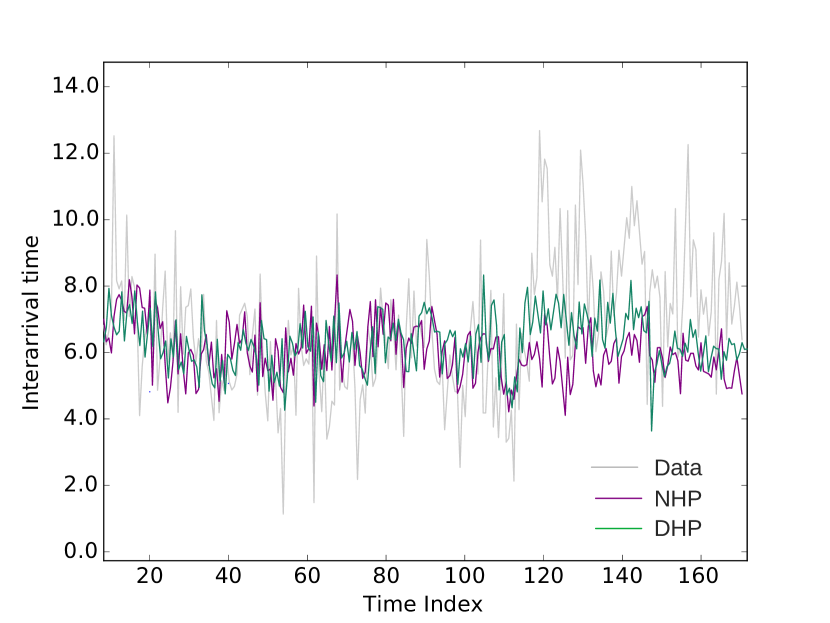
(a) Time Prediction Graph

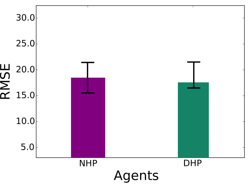
(b) Time Prediction Error

(c) Event Prediction Error

Figure 5: Performance evaluation of high-frequency market making agents in predicting order book events and time at nanosecond resolution. The standard deviation over 10 experiments using different train-val-test sample is denoted by error bar.

In Figure 6, we evaluate the predictive performance of the high-frequency market making agents using millisecond data sampled from the reconstructed order book. Compared to the earlier results, the DHP model’s performance has drastically increased. In addition, the time prediction is consistently better than with the NHP. The deep model with novel architecture and pre-training module are sophisticated enough to capture excitation and feedback effects in the order book. The results also substantiate the claim of the NHP model regarding stochastically missing data. The order book events at millisecond timestamps theoretically omit the events at the finer time resolution, but they are generated by a different mechanisms. This is the reason why there are completely different results at the two time resolutions. The Deep Hawkes model presented here is expressive enough to learn true predictive distribution with scholastically missing events, but only if they are generated from the same mechanism. By integrating the predictive capabilities into the market making strategies, the agents trade in a simulation framework populated with heterogeneous trading strategies. In the next section, we explore the agents’ trading performance.

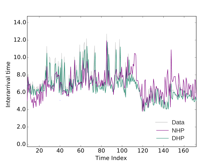
(a) Time Prediction Graph

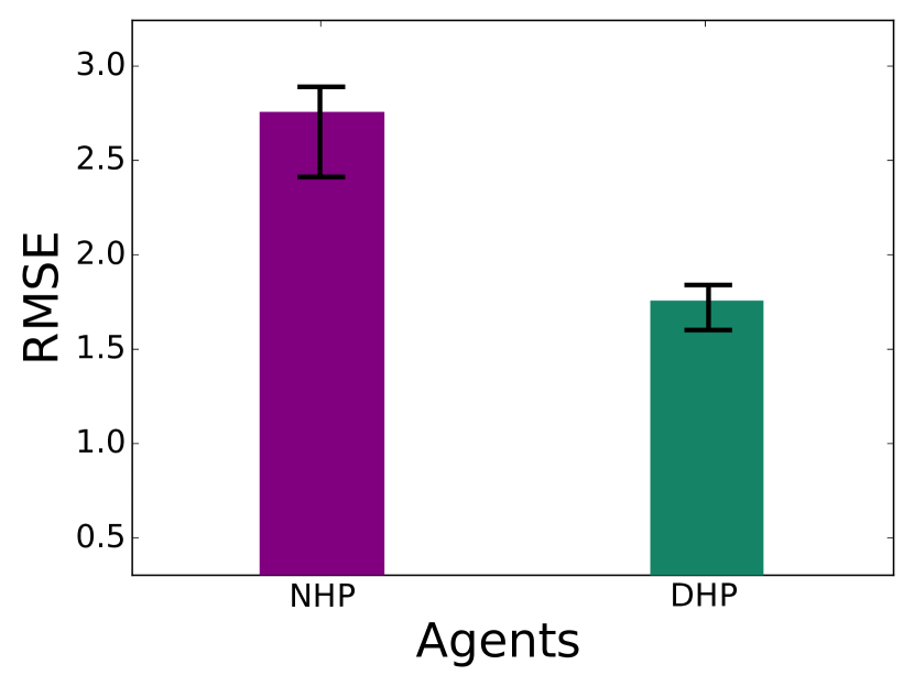
(b) Time Prediction Error

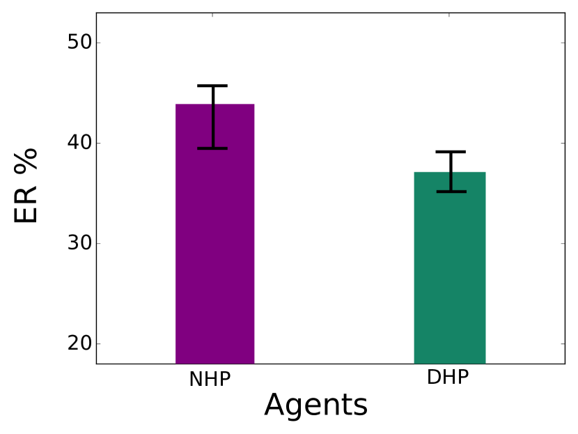
(c) Event Prediction Error

Figure 6: Performance evaluation of high-frequency market making agents in predicting order book events and time at millisecond resolution. The standard deviation over 10 experiments using different train-val-test sample is denoted by error bar.

7.2 Trading Performance

The trading performance of the high-frequency market making agents is discussed in Table 3. Our simulation framework evaluates various models, including the Neural Hawkes model, the benchmark probabilistic estimate model, and our proposed Deep Hawkes model. According to the performance metrics specified in Table 3, our proposed agent using DHP (DHMM) consistently outperforms the PMM and NHMM, which suggests that the proposed trading agent benefits by learning the robust microstructure of order book data. Further, the DHP lets the agent capture the self- and cross-excitation effects of the limit order book together with a feedback loop, to place the right order at the right time. We discuss the performance of each agent in detail below.

As shown in Figure 6, the DHMM is better at predicting the type of order and its time compared to NHMM. This is an important element of the market making strategy. The novel DLSTM-SDAE architecture allows the agents to learn the hidden representation of the noisy order book data, and therefore to place orders that add to its profitability. Furthermore, DHMM exhibits a faster convergence rate compared to NHMM, as shown in Figure 7.

The baseline strategy used by PMM maintains a probability density estimated on the basis of fundamental price. The fundamental price evolves according to the jump process, following a normal distribution. This works in the favor of PMM, which makes more profit at the beginning, as verified in Figure 7.Over time, however, the DHMM and NHMM learn the art of placing the right order with the right intensity. Afterwards, the profitability of the PMM fall dramatically. The PMM might perform better if it took a long position over several days, rather than trading intraday. It would be interesting to check the performance of the PMM agents with different probability density estimate conditions on the joint distribution of microstructure features.

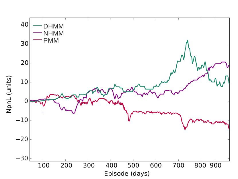
(a) Train

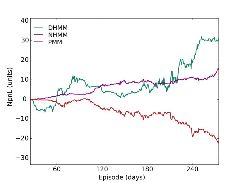
(b) Test

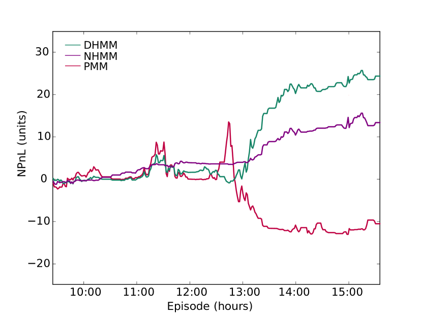
(c) Random day

Figure 7: Trading agents performance with DHMM, NHMM and PMM while training, testing and random day.

Table 3: Mean and standard deviation on the daily normalised PnL (PnL) and mean absolute positions (MAP) for different market makers

Agents	NPnL [$10^{5}$]		MAP[unit]
	Mean	Std.Dev.	Mean	Std.Dev.
DHMM	2.1	$\pm 18.26$	17	$\pm 20$
NHMM	1.1	$\pm 4.09$	4	$\pm 6$
PMM	-1.6	$\pm 79.55$	41	$\pm 74$

7.3 Order Cancellation Effect

Massive numbers of order cancellations in a short period are a distinctive attribute of the equity market. For example, at Nasdaq Nordic, order cancellations typically account for 40% of submitted limit orders on a particular trading day. Market making strategies using limit order cancellations contribute to the market marker’s profit, bid-ask spread and order queue position (Dahlström et al.,, 2018).We study the distribution of profit, bid-ask spread and order queue position by removing the cancellations mechanism in the base simulation framework. We estimate the intrinsic value of the order relative to the queue position by applying the model developed by Moallemi and Yuan, (2017). The agent’s order queue position provides an estimate of number of orders ahead of the agent’s order at a particular price. A position at the front of the queue guarantees prompt execution, higher fill rate, low latency and lower adverse selection cost. We estimate the queue position in the order book by reconstructing the limit order book from the simulated data feed.

Lets us suppose that the high-frequency market making agent places a limit order at time $t\!=0$ seeking best ask price $p_{a}$ which gets filled or canceled at time $\tau$. Filling the order pays the agent $p_{a}$ while cancellations pay nothing. We now describe the value of the order perceived by agents relative to the queue position as:

$$\begin{split}V_{t}&=\mathbb{E}[(p_{a}-p_{t})\mathbb{I}_{\mathsf{FILL}}-(p-p_{t})\mathbb{I}_{\mathsf{FILL}}\mid\mathcal{F}_{t}]\\ &=\mathsf{FP}_{t}(\mathsf{LSP}_{t}-\mathsf{ASC}_{t})\\ &=fill\;probablity\left(liquidity\;spread\;premium-adverse\;selection\;cost\right)\end{split}$$ (7.1)

where

$$\begin{aligned} \!&\mathsf{FP}_{t}\triangleq\mathbb{P}\left(\mathsf{FILL}\mid\mathcal{F}_{t}\right),\\ \!&\mathsf{LSP}_{t}\triangleq\left(p_{a}-p_{t}\right),\\ \!&\mathsf{ASC}_{t}\triangleq\mathbb{E}\left[(p_{\tau}-p_{t})\mid\mathcal{F}_{t},\mathsf{FILL}\right]\end{aligned}$$

To empirically calibrate the model (Equation 7.1), we take the same parameters used by Moallemi and Yuan, (2017). These are exponential order size distribution, trade arrival rate (TAR), average trades size (ATS), trade size in the stan-dard lot (TSS), cancellation arrival rate (CAR), average cancellation size (ACS), price jump arrival rate (PJR), average jump size (AJS), market impact (MI) and average queue size (AQS). The trade size is identified as the limit order or market order, contrary to aggressive market orders as described by Moallemi and Yuan, (2017). Table 4 specifies the estimated parameters for simulated data with no cancellation mechanisms (Simulated NC), without cancellation mechanisms (Simulated WC) and an average (Simulated AV) over 21 days. The paper itself provides more detail regarding the parameters, calibration and model fitting (Moallemi and Yuan,, 2017).

Table 4: Estimated parameters for simulated orderbook data.

Data	TAR (/min)	ATS (shares)	TSS (shares)	CAR (/min)	ACS (shares)	PJR (/min)	AJS (ticks)	MI	AQS (shares)
Simulated NC	2.53	3467	7664	92.72	5061	1.26	0.32	10.91	16416
Simulated AV	2.04	4037	6901	82.21	4022	1.01	0.46	8.76	23554
Simulated WC	5.26	6329	8083	43.71	1107	3.75	2.06	11.92	40191
Simulated AV	4.07	5463	9147	40.31	1560	3.01	2.06	13.02	46815

Table 4 shows that an absence of cancellation mechanisms at the high-frequency market maker’s end leads to a drastic increase in the average queue size. The decrease in the cancellation rate increases the queue size, which affects the high-frequency market maker’s profitability, bid-ask spread and market impact. The value of the order as a function of the queue position, bid-ask spread, and the agent’s profit efficiently captures the claim illustrated by the data in Figure 8. The wider bid-ask spread when agent’s are unable to cancel the limit order in Figure 8(d) has negative effect on the profitability (Figure 8(e) ) as compared to scenarios with cancellations (Figure 8(a),8(b) ). As stated in the model in Equation 7.1, the value of an order that is not filled is zero. Figure 8(f) shows that an increase in queue length decreases the probability of execution, and therefore the value. The value of the order becomes flat, as the queue length is extremely large. Our results are consistent with the findings of Dahlström et al., (2018) when investigating the determinants of order cancellations. It is difficult to infer causal relationships between cancellations and market microstructure variables based on artificially created scenarios, but this approach nonetheless it paves the way for future investigation using order level data.

(a) BAD WC

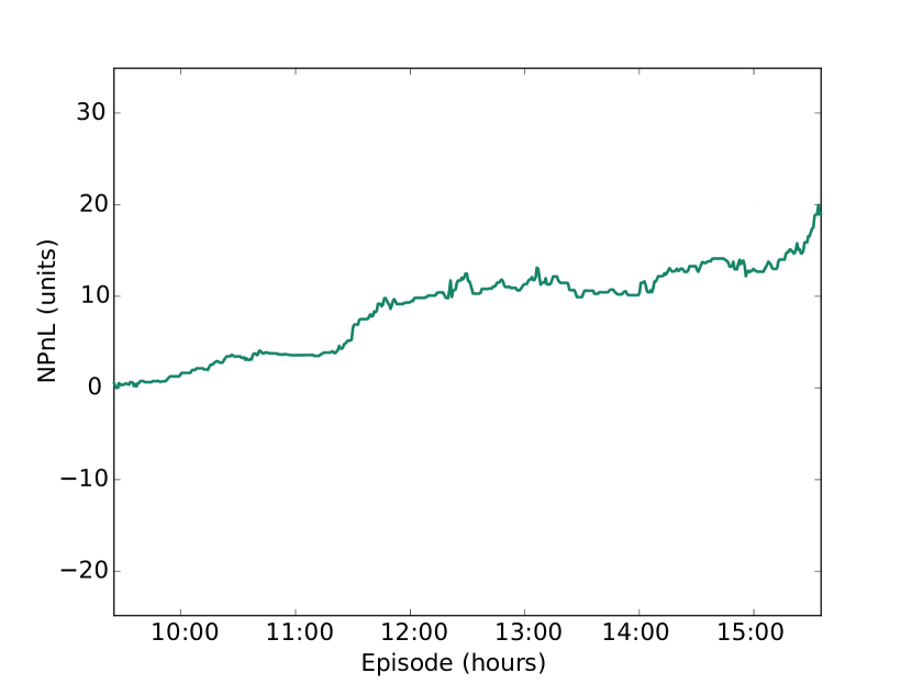
(b) DHMMP WC

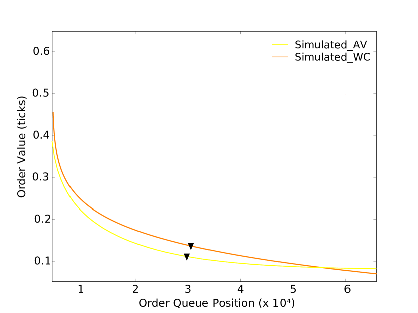
(c) VOPQ WC

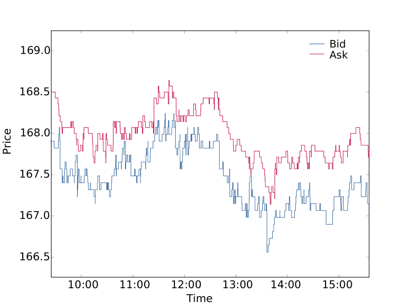
(d) BAD NC

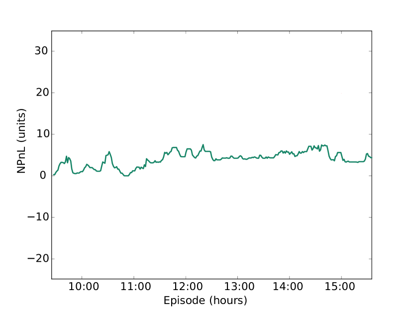
(e) DHMMP NC

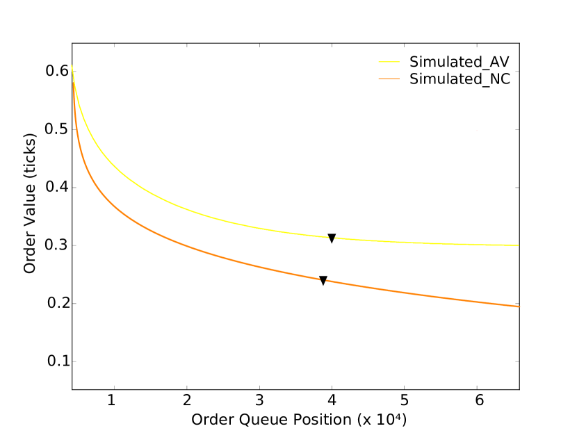
(f) VOPQ NC

Figure 8: Effect of limit order cancellations on the market. The top row (marked WC) represents the distribution when the market maker’s agents can cancel the limit orders. The bottom row (marked NC) represents a situation with no cancellations. BAD is intraday bid-ask distribution, DHMMP is profit distribution of DHMM over the trading day, and VOPQ is the value of the orders relative to queue position. The average queue length on a particular trading day is represented by a black triangle.

7.4 Sensitivity Analysis

We perform sensitivity analysis on the proposed model by changing the hyperparameters – specifically, the number of layers, the number of hidden units per layer and the noise level. The aim is to confirm the robustness of the model, rather than overfitting parameters. Table 5 shows the performance of our proposed model when there is an increase in the number of layers, hidden units and noise level. The model is robust to the noise level at the optimal choice of numbers of layers, parameters and hidden units.

Table 5: Sensitivity to the number of hidden units and Gaussian noise. The DLSTM-SDAE used in our model has 3 DAE layers and 3 LSTM layers. In performing sensitivity analysis, we fix the 3 LSTM layers and change only the DAE layer.

	# Number of layer 1	# Number of layer 2	# Number of layer 3
Number of hidden unit per layer	$\left(64,128,256,512,1024\right)$	$\left(64,128,256,512,1024\right)$	$\left(64,128,256,512,1024\right)$
RMSE	$\left(4.6,4.4,4.1,4.1,4.0\right)$	$\left(3.5,3.0,3.0,2.5,2.5\right)$	$\left(2.0,2.0,2.0,1.5,1.5\right)$
ER	$\left(55.7,55.7,55.7,50.4,54.0\right)$	$\left(47.2,44.4,44.1,44.1,44.1\right)$	$\left(37.5,37.0,35.0,35.0,34.0\right)$
Gaussian noise	$\left(0.10,0.20,0.30,0.40,0.50\right)$	$\left(0.10,0.20,0.30,0.40,0.50\right)$	$\left(0.10,0.20,0.30,0.40,0.50\right)$
RMSE	$\left(7.2,5.9,4.3,5.4,6.5\right)$	$\left(4.1,3.9,3.0,4.0,4.6\right)$	$\left(2.2,2.2,2.0,2.1,2.1\right)$
ER	$\left(60.2,55.9,50.1,60.0,63.5\right)$	$\left(55.6,52.2,49.1,55.3,67.5\right)$	$\left(37.2,37.9,37.3,37.1,37.2\right)$

7.5 Validation

The validation of the trading simulation framework is performed by measuring how successfully the simulation’s output exhibits persis- tent empirical patterns in the order book data. Such empirical patterns are common across various markets and instruments, and even timescales are often classified as ”stylised facts” (Cont,, 2001). We present a nominal set of stylised facts, reproduced from the empirical analysis of simulated order book data, as shown in Figure 9.

Let $p(t)$ be the price of a security at time $t$. Given a timescale $\Delta t$, we define log return at $\Delta t$ as $r(t,\Delta t)=\ln p(t+\Delta t)-\ln p(t)$. The cumulative distribution (CDF) of returns is given as $F_{\Delta t}(x)=\mathbb{P}[r(t,\Delta t)\leq x]$. The derivative of the earlier gives probability density function (PDF) $F^{{}^{\prime}}_{\Delta t}=f_{\Delta t}$, empirically estimated for normalized simulated return, as illustrated in Figure 9(a). The cumulative distribution of return follows power law $F_{\Delta t}\sim\left|r\right|^{-\alpha}$ with $2<\alpha<5$. In Figure 9(b), the positive tail $F^{+}_{\Delta t}(x)=\mathbb{P}[r(t,\Delta t)\geq x]$ and the negative tail $F^{-}_{\Delta t}(x)=\mathbb{P}[r(t,\Delta t)\leq x]$ of cumulative distribution, shown as yellow circles and green squares, exhibit power law, as denoted by the red line with $\alpha=2.8$. In Figure 9(c), we show the absence of the autocorrelation of price change, defined as $\rho(\tau)=Corr\left(r(t,\Delta t),r(t+\tau,\Delta t)\right)$. The autocorrelation function (ACF) drastically decays to zero in few lags.

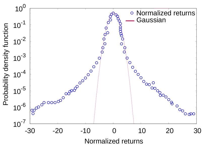
(a) PDF

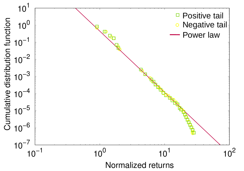
(b) CDF

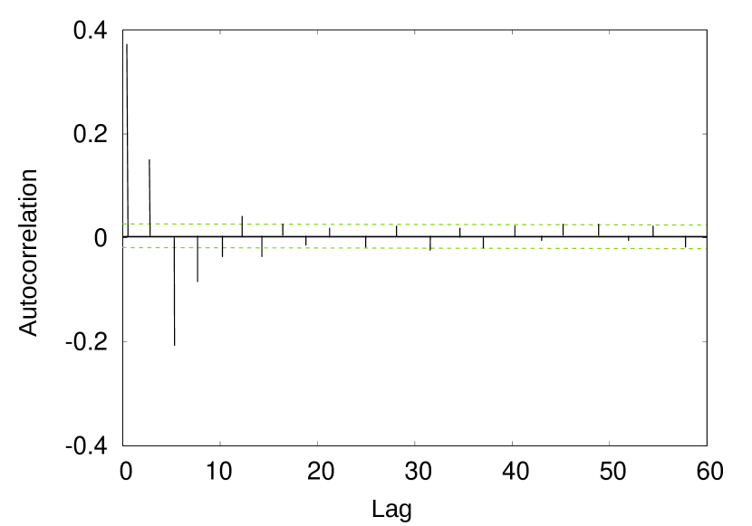
(c) ACF

Figure 9: Stylised facts reproduced from simulated order book data. All graphs were generated on the basis of $\Delta t=1\;minute$.

8 Conclusions

We have developed a market making strategy that takes account of the feedback loop between the order arrival and the state of the LOB, with self- and cross-excitation effects, while placing an order in our realistic simulation framework. The strategy was designed by integrating the self-modulating multivariate Hawkes process with DLSTM-SDAE. The data-driven approach performed adversely in relation to predicting the next order type and its timestamp when fitted to reconstructed order book data at nanosecond resolution. When trained with millisecond resolution data, it outperforms NHP in prediction tasks and benchmark market making strategies in trading performance. We have demonstrated that extending the DHP in a market making setting accomplished better performance when validating empirical claims about the effect of cancellation on the determinants of order size. Our modelling approach is still far from inferring causality, but does pave the way exploring a range of diverse research avenues. The most important and immediate of these are listed below:

1. Apply more advanced pre-processing, architecture, and learning algorithms to filter out ultra-noisy order book data at nanosecond timestamps.

2. Explore an intensity-free approach for Hawkes processes with learning mechanisms other than the maximum likelihood approach.

3. Embedding DHP within the reinforcement learning framework to learn the optimal policy.

4. Extend the model to the deep reinforcement learning framework, in which the agent’s trading action and reward from the simulator are asynchronous stochastic events characterised by marked multivariate Hawkes processes.

5. Extract the agent’s trading algorithm parameters directly from the order book data , rather than from random seeds or empirical literature.

References

- Ait-Sahalia and Saglam, (2017) Ait-Sahalia, Y. and Saglam, M. (2017). High frequency market making: Implications for liquidity. SSRN Electronic Journal.
- Arras et al., (2019) Arras, L., Arjona-Medina, J., Widrich, M., Montavon, G., Gillhofer, M., Müller, K.-R., Hochreiter, S., and Samek, W. (2019). Explaining and interpreting lstms. In Samek, W., Montavon, G., Vedaldi, A., Hansen, L. K., and Müller, K.-R., editors, Explainable AI: Interpreting, Explaining and Visualizing Deep Learning, pages 211–238, Cham. Springer International Publishing.
- Avellaneda and Stoikov, (2008) Avellaneda, M. and Stoikov, S. (2008). High frequency trading in a limit order book. Quantitative Finance, 8:217–224.
- Bacry et al., (2015) Bacry, E., Mastromatteo, I., and Muzy, J.-F. (2015). Hawkes processes in finance. Market Microstructure and Liquidity, 01(01):1550005.
- Brogaard et al., (2014) Brogaard, J., Hendershott, T., and Riordan, R. (2014). High-frequency trading and price discovery. The Review of Financial Studies, 27(8):2267–2306.
- Cartea et al., (2014) Cartea, Á., Jaimungal, S., and Ricci, J. (2014). Buy low, sell high: A high frequency trading perspective. SIAM Journal on Financial Mathematics, 5(1):415–444.
- Chakraborti et al., (2011) Chakraborti, A., Muni Toke, I., Patriarca, M., and Abergel, F. (2011). Econophysics review: I. empirical facts. Quantitative Finance, 11(7):991–1012.
- Chakraborty and Kearns, (2011) Chakraborty, T. and Kearns, M. (2011). Market making and mean reversion. In Proceedings of the 12th ACM Conference on Electronic Commerce, page 307–314, New York, NY, USA. Association for Computing Machinery.
- Chao et al., (2018) Chao, Y., Yao, C., and Ye, M. (2018). Why Discrete Price Fragments U.S. Stock Exchanges and Disperses Their Fee Structures. The Review of Financial Studies, 32(3):1068–1101.
- Clauset et al., (2009) Clauset, A., Shalizi, C. R., and Newman, M. E. J. (2009). Power-law distributions in empirical data. SIAM Review, 51(4):661–703.
- Cont, (2001) Cont, R. (2001). Empirical properties of asset returns: stylized facts and statistical issues. Quantitative Finance, 1(2):223–236.
- Cont and Sirignano, (2019) Cont, R. and Sirignano, J. (2019). Universal features of price formation in financial markets: perspectives from deep learning. Quantitative Finance, 19(9):1449–1459.
- Dahlström et al., (2018) Dahlström, P., Hagströmer, B., and Norden, L. L. (2018). Determinants of limit order cancellations. Microeconomics: General Equilibrium and Disequilibrium Models of Financial Markets eJournal, pages 1–57.
- Das, (2005) Das, S. (2005). A learning market-maker in the glosten-milgrom model. Quantitative Finance, 5(2):169–180.
- Du et al., (2016) Du, N., Dai, H., Trivedi, R., Upadhyay, U., Gomez-Rodriguez, M., and Song, L. (2016). Recurrent marked temporal point processes: Embedding event history to vector. In Proceedings of the 22nd ACM SIGKDD International Conference on Knowledge Discovery and Data Mining, KDD ’16, page 1555–1564, New York, NY, USA. Association for Computing Machinery.
- Embrechts et al., (2011) Embrechts, P., Liniger, T., and Lin, L. (2011). Multivariate hawkes processes: an application to financial data. Journal of Applied Probability, 48(A):367–378.
- Farmer, (2002) Farmer, J. D. (2002). Market force, ecology and evolution. Industrial and Corporate Change, 11(5):895–953.
- Ganesh et al., (2019) Ganesh, S., Vadori, N., Xu, M., Zeng, H., Reddy, P., and Veloso, M. (2019). Reinforcement learning for market making in a multi-agent dealer market.
- Gao et al., (2018) Gao, X., Zhou, X., and Zhu, L. (2018). Transform analysis for hawkes processes with applications in dark pool trading. Quantitative Finance, 18(2):265–282.
- Glosten and Milgrom, (1985) Glosten, L. and Milgrom, P. (1985). Bid, ask and transaction prices in a specialist market with heterogeneously informed traders. Journal of Financial Economics, 14(1):71 – 100.
- Gonzalez and Schervish, (2017) Gonzalez, F. and Schervish, M. (2017). Instantaneous order impact and high-frequency strategy optimization in limit order books. Market Microstructure and Liquidity, 03(02):1850001.
- Gould et al., (2013) Gould, M., Porter, M., Williams, S., McDonald, M., Fenn, D., and Howison, S. (2013). Limit order books. Quantitative Finance, 13(11):1709–1742.
- Guéant et al., (2013) Guéant, O., Lehalle, C.-A., and Fernandez-Tapia, J. (2013). Dealing with the inventory risk: A solution to the market making problem. Mathematics and Financial Economics, 7:477–507.
- Gueant and Manziuk, (2019) Gueant, O. and Manziuk, I. (2019). Deep reinforcement learning for market making in corporate bonds: Beating the curse of dimensionality. Applied Mathematical Finance, 26(5):387–452.
- Hawkes, (2018) Hawkes, A. (2018). Hawkes processes and their applications to finance: a review. Quantitative Finance, 18(2):193–198.
- Ho and Stoll, (1981) Ho, T. and Stoll, H. (1981). Optimal dealer pricing under transactions and return uncertainty. Journal of Financial Economics, 9(1):47 – 73.
- Hochreiter and Schmidhuber, (1997) Hochreiter, S. and Schmidhuber, J. (1997). Long short-term memory. Neural computation, 9(8):1735–1780.
- Huang and Polak, (2011) Huang, R. and Polak, T. (2011). Lobster: Limit order book reconstruction system. SSRN Electronic Journal.
- Huang et al., (2015) Huang, W., Lehalle, C.-A., and Rosenbaum, M. (2015). Simulating and analyzing order book data: The queue-reactive model. Journal of the American Statistical Association, 110(509):107–122.
- Hyndman and Koehler, (2006) Hyndman, R. and Koehler, A. (2006). Another look at measures of forecast accuracy. International Journal of Forecasting, 22(4):679 – 688.
- Izumi and Toriumi, (2009) Izumi, K. and Toriumi, F.and Matsui, H. (2009). Evaluation of automated-trading strategies using an artificial market. Neurocomputing, 72(16):3469 – 3476.
- Kingma and Ba, (2015) Kingma, D. and Ba, J. (2015). Adam: A method for stochastic optimization. In 3rd International Conference on Learning Representations, ICLR 2015,San Diego, CA, USA, May 7-9, 2015, Conference Track Proceedings.
- Kirilenko et al., (2017) Kirilenko, A., Kyle, A., SAMADI, M., and Tuzun, T. (2017). The flash crash: High frequency trading in an electronic market. The Journal of Finance, 72(3):967–998.
- Kumar, (2020) Kumar, P. (2020). Deep reinforcement learning for market making. In Proceedings of the 20th International Conference on Autonomous Agents and MultiAgent Systems, AAMAS ’20, page 1892–1895, Richland, SC. International Foundation for Autonomous Agents and Multiagent Systems.
- Leal et al., (2016) Leal, S. J., Napoletano, M., Roventini, A., and Fagiolo, G. (2016). Rock around the clock: An agent-based model of low- and high-frequency trading. Journal of Evolutionary Economics volume, 26:49–76.
- Li et al., (2019) Li, Y., Zheng, W., and Zheng, Z. (2019). Deep robust reinforcement learning for practical algorithmic trading. IEEE Access, 7:108014–108022.
- Lu and Abergel, (2018) Lu, X. and Abergel, F. (2018). Order-book modeling and market making strategies. Market Microstructure and Liquidity, 04(01n02):1950003.
- Maeda et al., (2020) Maeda, I., deGraw, D., Kitano, M., Matsushima, H., Sakaji, H., Izumi, K., and Kato, A. (2020). Deep reinforcement learning in agent based financial market simulation. Journal of Risk and Financial Management, 13(4):1–17.
- Mankad and Michailidis, (2013) Mankad, S. and Michailidis, G. (2013). Discovering the ecosystem of an electronic financial market with a dynamic machine-learning method. Algorithmic Finance, 2(2):151–165.
- McGroarty et al., (2019) McGroarty, F., Booth, A., Gerding, E., and Chinthalapati, V. L. R. (2019). High frequency trading strategies, market fragility and price spikes: an agent based model perspective. Annals of Operations Research, 282(1):217–244.
- Mei and Eisner, (2017) Mei, H. and Eisner, J. (2017). The neural hawkes process: A neurally self-modulating multivariate point process. In Proceedings of the 31st International Conference on Neural Information Processing Systems, NIPS’17, page 6757–6767, Red Hook, NY, USA. Curran Associates Inc.
- Menkveld, (2013) Menkveld, A. (2013). High frequency trading and the new market makers. Journal of Financial Markets, 16:712–740.
- Mnih et al., (2015) Mnih, V., Kavukcuoglu, K., Silver, D., Rusu, A. A., Veness, J., Bellemare, M. G., Graves, A., Riedmiller, M., Fidjeland, A. K., Ostrovski, G., Petersen, S., Beattie, C., Sadik, A., Antonoglou, I., King, H., Kumaran, D., Wierstra, D., Legg, S., and Hassabis, D. (2015). Human-level control through deep reinforcement learning. Nature, 518(7540):529–533.
- Moallemi and Yuan, (2017) Moallemi, C. C. and Yuan, K. (2017). A model for queue position valuation in a limit order book. Technical report, Columbia Business School Research Paper No. 17-70.
- Morariu-Patrichi and Pakkanen, (2018) Morariu-Patrichi, M. and Pakkanen, M. S. P. (2018). State-dependent hawkes processes and their application to limit order book modelling.
- Mu et al., (2009) Mu, G.-H., Chen, W., Kertész, J., and Zhou, W.-X. (2009). Preferred numbers and the distributions of trade sizes and trading volumes in the chinese stock market. Physics of Condensed Matter, 68:145–152.
- Mukerji et al., (2019) Mukerji, P., Chung, C., Walsh, T., and Xiong, B. (2019). The impact of algorithmic trading in a simulated asset market. Journal of Risk and Financial Management, 12:68.
- Muni Toke, (2011) Muni Toke, I. (2011). ”market making” in an order book model and its impact on the spread. In Abergel, F., Chakrabarti, B. K., Chakraborti, A., and Mitra, M., editors, Econophysics of Order-driven Markets: Proceedings of Econophys-Kolkata V, pages 49–64, Milano. Springer Milan.
- Musciotto et al., (2018) Musciotto, F., Marotta, L., Piilo, J., and Mantegna, R. (2018). Long-term ecology of investors in a financial market. Palgrave Communications, 4:92.
- Nasdaq, (2020) Nasdaq (2020). Nasdaq totalview-itch 5.0. http://www.nasdaqtrader.com/content/technicalsupport/specifications/dataproducts/NQTVITCHSpecification.pdf. accessed: 21.07.2020.
- Nystrom et al., (2014) Nystrom, K., Ould Aly, S. M., and Zhang, C. (2014). Market making and portfolio liquidation under uncertainty. International Journal of Theoretical and Applied Finance, 17(05):1450034.
- O’Hara and Oldfield, (1986) O’Hara, M. and Oldfield, G. S. (1986). The microeconomics of market making. Journal of Financial and Quantitative Analysis, 21(4):361–376.
- Paulin et al., (2019) Paulin, J., Calinescu, A., and Wooldridge, M. (2019). Understanding flash crash contagion and systemic risk: A micro–macro agent-based approach. Journal of Economic Dynamics and Control, 100:200 – 229.
- Penalva et al., (2015) Penalva, J., Cartea, A., and Jaimungal, s. (2015). Algorithmic and High-Frequency Trading. Cambridge University Press, first edition.
- Preis et al., (2006) Preis, T., Golke, S., Paul, W., and Schneider, J. (2006). Multi-agent-based order book model of financial markets. Europhysics Letters (EPL), 75(3):510–516.
- Rambaldi et al., (2017) Rambaldi, M., Bacry, E., and Lillo, F. (2017). The role of volume in order book dynamics: a multivariate hawkes process analysis. Quantitative Finance, 17(7):999–1020.
- (57) Sagheer, A. and Kotb, M. (2019a). Time series forecasting of petroleum production using deep lstm recurrent networks. Neurocomputing, 323:203 – 213.
- (58) Sagheer, A. and Kotb, M. (2019b). Unsupervised pre-training of a deep lstm-based stacked autoencoder for multivariate time series forecasting problems. Scientific Reports, 9:19038.
- Samanidou et al., (2007) Samanidou, E., Zschischang, E., Stauffer, D., and Lux, T. (2007). Agent-based models of financial markets. Reports on Progress in Physics, 70(3):409–450.
- Sandas, (2001) Sandas, P. (2001). Adverse selection and competitive market making: Empirical evidence from a limit order market. The Review of Financial Studies, 14(3):705–734.
- SEC, (2014) SEC (2014). Equity market structure literature review part ii: High frequency trading, pages 63–103. U.S. Securities and Exchange Commission, Staff of the Division of Trading and Markets.
- Silver et al., (2017) Silver, D., Schrittwieser, J., Simonyan, K., Antonoglou, I., Huang, A., Guez, A., Hubert, T., Baker, L., Lai, M., Bolton, A., Chen, Y., Lillicrap, T., Hui, F., Sifre, L., van den Driessche, G., Graepel, T., and Hassabis, D. (2017). Mastering the game of go without human knowledge. Nature, 550:354–.
- Sirignano, (2019) Sirignano, J. (2019). Deep learning for limit order books. Quantitative Finance, 19(4):549–570.
- Smith et al., (2003) Smith, E., Farmer, D., Gillemot, L., and Krishnamurthy, S. (2003). Statistical theory of the continuous double auction. Quantitative Finance, 3(6):481–514.
- Spooner et al., (2018) Spooner, T., Fearnley, J., Savani, R., and Koukorinis, A. (2018). Market making via reinforcement learning. In Proceedings of the 17th International Conference on Autonomous Agents and MultiAgent Systems, AAMAS ’18, page 434–442, Richland, SC. International Foundation for Autonomous Agents and Multiagent Systems.
- Tashiro et al., (2019) Tashiro, D., Matsushima, H., Izumi, K., and Sakaji, H. (2019). Encoding of high-frequency order information and prediction of short-term stock price by deep learning. Quantitative Finance, 19(9):1499–1506.
- Toth et al., (2012) Toth, B., Eisler, Z., Lillo, F., Kockelkoren, J., Bouchaud, J., and Farmer, J. (2012). How does the market react to your order flow? Quantitative Finance, 12(7):1015–1024.
- Tsantekidis et al., (2017) Tsantekidis, A., Passalis, N., Tefas, A., Kanniainen†, J., Gabbouj, M., and Iosifidis, A. (2017). Using deep learning to detect price change indications in financial markets. In 2017 25th European Signal Processing Conference (EUSIPCO), pages 2511–2515.
- Vincent et al., (2010) Vincent, P., Larochelle, H., Lajoie, I., Bengio, Y., and Manzagol, P.-A. (2010). Stacked denoising autoencoders: Learning useful representations in a deep network with a local denoising criterion. J. Mach. Learn. Res., 11:3371–3408.
- Wah et al., (2017) Wah, E., Wright, M., and Wellman, M. (2017). Welfare effects of market making in continuous double auctions. J. Artif. Int. Res., 59(1):613–650.
- Zhang et al., (2019) Zhang, Z., Zohren, S., and Roberts, S. (2019). DeepLOB: Deep convolutional neural networks for limit order books. IEEE Transactions on Signal Processing, 67(11):3001–3012.
- Zhu et al., (2016) Zhu, W., Lan, C., Xing, J., Zeng, W., Li, Y., Shen, L., and Xie, X. (2016). Co-occurrence feature learning for skeleton based action recognition using regularized deep lstm networks. In Proceedings of the Thirtieth AAAI Conference on Artificial Intelligence, AAAI’16, page 3697–3703. AAAI Press.