Klein tunneling through double barrier in ABC-trilayer graphene

Abstract

Klein tunneling and conductance for Dirac fermions in ABC-stacked trilayer graphene (ABC-TLG) through symmetric and asymmetric double potential barrier are investigated using the two and six-band continuum model. Numerical results for our system show that the transport is sensitive to the height, the width and the distance between the two barriers. Klein paradox at normal incidence and resonant features at non-normal incidence in the transmission result from resonant electron states in the wells or hole states in the barriers and strongly influence the ballistic conductance of the structures.

I Introduction

Generally, grapheneNovoselov2004 ; Novoselov2005 ; Zhang2005 ; Geim is a two dimensional (2D) lattice of carbon atoms arranged in hexagonal geometry. Its stacking can be realized in different methods to engineer multi-layered graphene showing various physical properties. Typical examples of stacking includes Order, Bernal (AB), and Rhombohedral stacking (ABC)Aoki2007 ; Dresselhaus200286 ; Jhang11 ; Koshino2010 ; Lui11 ; Koshino200923 . In the first one all carbon atoms of each layer are well-aligned, while the second and third ones having cycle periods composed of two layers and three layers of non-aligned graphene, respectively. It has been showed that the band structure, Klein tunneling, band gap, transport and optical properties of graphene depend on the way how it is stacked Latil2006 ; Koshino2010 ; Mikito2013 ; Aoki2007 ; Cocemasov2013 ; Mak2010 ; Guinea200626 ; Avetisyan200901 ; Avetisyan201032 ; Lu200627 ; Ben201301 ; Chegel201683 ; Sheng200966 ; Celal2016 and the applied external sources Aoki2007 ; Koshino2010 ; Kumar201101 ; Katsnelson2006 ; Peeters2010 ; Kumar2012 ; CommentBen ; vanduppen205427 ; Ben201301 ; vanduppen195439 ; Pereira ; Mirzakhani2017 ; ElMouhafid2017 ; Benlakhouy114835 .

One of the latest focuses a few of the multi-layer structures is the trilayer graphene (TLG)Guinea200626 ; Mirzakhani2017 ; Craciun2009 ; Kumar2012 ; vanduppen195439 ; Ben201301 ; Koshino2009 ; Zhang2010 ; Sena2011 ; Zhang2013 ; Jung2013 ; SalahUddin2014 ; Marcos2014 ; Ma2012 ; Yuan2011 ; Menezes2014 ; Yin2017 ; Barlas2012 ; Cote2012 ; Xu2015 ; Yun2016 ; Kumar2014 , which has two distinct allotropes such that the Bernal (ABA) and Rhombohedral (ABC) stackings. For ABA we have atoms of the top layer lie exactly on top of the bottom layer in addition to a dispersion relation as a combination of the single layer linear energy band and the quadratic dispersion of bilayer graphene with no opening gap under applied external electric fieldLui2011 . While ABC has atoms of one of the sublattices of topmost layer lie above the center of the hexagons of bottom layer and shows a dispersion relation approximately cubic with conduction and valence bands touching each other at a point close to the highly symmetric $\mathbf{K}$ and $\mathbf{K^{\prime}}$ pointsAoki2007 ; Zhang2010 . Consequently, the way in which the layers are stacked modifies strongly the energy spectrum of the resulted system and this of course affects its transport properties as well. Moreover, for TLG it was showed that the emergence of a Klein tunneling strongly depends on the staking order, being present only in ABC-TLGKumar2012 ; CommentBen ; Ben201301 . Experimentally, the transport properties of ABC- and ABA-TLG using dual locally gated field effect devices was investigated Zhang2013 where an opening of a band gap was observed. The giant conductance oscillations in ballistic TLG Fabry-Pérot interferometers was realized Campos2012 , which came as a result from the phase coherent transport through resonant bound states subjected to an electrostatic barrier.

Motivated by different achievements listed above, especially Kumar2012 ; CommentBen ; Ben201301 , we study the Kelin tunneling of Dirac fermions in ABC-TLG scattered by a square double barrier. More precisely, the transmission probabilities and conductance of electrons will be investigated by tacking into account the full six band energy spectrum. We analyze two interesting cases by making comparison between the incident energy $E$ and interlayer coupling parameter $\gamma_{1}$. Indeed, for $E<\gamma_{1}$ there is only one channel of transmission exhibiting resonances, even for incident particles of energy $E$ less than the barrier heights $V_{j}$, i.e. $E<V_{j}$, depending on the double barrier profile. For $E>\gamma_{1}$, we end up with tree propagating modes resulted from nine possible ways of transmission. Subsequently, we use the transfer matrix and density of current to determine all transmission channels together with the conductance associated to our system. Under the appropriate choices of the physical parameters characterizing our system, we numerically analyze our results and compare them with literature.

The outline of the present paper is as follows. In section II, we establish a mathematical framework using the full band model to determine the eigenvalues and eigenvectors through double barrier. In section III, by matching the eigenspinors of different regions at interfaces and using the transfer matrix together with the current density, we obtain nine channels of transmission and reflections as well as the associated conductance. We study two band tunneling for symmetric and asymmetric barrier with and without the interlayer potential difference. At high energy, we repeat the same task but by considering full band and emphasis what makes difference with respect to other case. In section IV, we numerically study the basics features of the resulted conductance and show the effect of symmetric and asymmetric barrier. Finally, we briefly summarize our main findings.

II Theory formula

II.1 Eigenvalues and eigenvectors

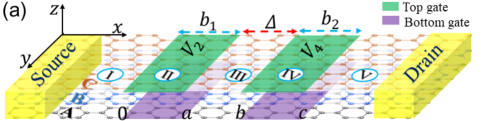
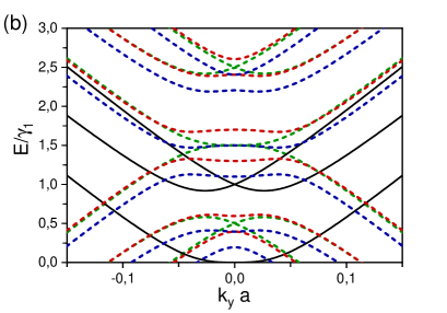
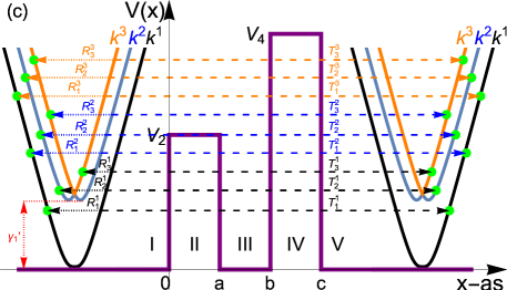
Figure 1: (Color online) Tunneling through a double barrier potential in ABC-TLG graphene. (a): Profile of a rectangular double barrier applied to our system. Indeed, an electrostatic potential difference $2\delta$ between top and bottom layers is applied in region II and IV. While, the electrostatic potential equal $V_{2}$ and $V_{4}$ for all three layers are applied in region II and IV, respectively. A, B, and C are three distinct positions of the hexagonal lattice when graphene trilayers are stacked. (b): Energy as function of the momentum $k_{y}$. $V_{2}=V_{4}=1.5\gamma_{1}$ and $\delta_{2}=\delta_{4}=0$ (green lines). $V_{2}=V_{4}=1.5\gamma_{1}$ and $\delta_{2}=\delta_{4}=0.2\gamma_{1}$ (red lines). $V_{2}=1.3\gamma_{1}$, $V_{4}=1.5\gamma_{1}$ and $\delta_{2}=\delta_{4}=0.2\gamma_{1}$ (blue lines). The dashed and thick lines represent the band inside and outside the barriers, respectively. (c): Schematic representation of different modes as well as the corresponding transmission and reflection channels. The dots and arrows indicate the energy regions for which electrons impinging perpendicularly on the barrier will be transmitted or reflected. We have chosen $\gamma^{\prime}_{1}=0.918\gamma_{1}.$

Single layer graphene (SLG) has a hexagonal crystal structure of two sublattices A and B with the interatomic distance $a=0.142$ nm Partoens2007 and the intra-layer coupling $\gamma_{0}\approx 3$ eVZhang2011 . On the other hand, TLG graphene is a tree stacked SLG (Rhombohedral stacking) and has an unit cell of six atomsCote2013 . Under the nearest-neighbor tight binding approximation, one can derive the Hamiltonian describing ABC-TLG near the $\mathbf{K}$ point Zhang2010

$$H=\hbar v_{F}\begin{pmatrix}\boldsymbol{\sigma}\cdot\boldsymbol{k}&\Gamma&0\\ \Gamma^{{\dagger}}&\boldsymbol{\sigma}\cdot\boldsymbol{k}&\Gamma\\ 0&\Gamma^{{\dagger}}&\boldsymbol{\sigma}\cdot\boldsymbol{k}\end{pmatrix},$$ (1)

in the basis of the atomic orbital eigenfunctions

$$\Psi=\left(\psi_{A_{1}},\psi_{B_{1}},\psi_{A_{2}},\psi_{B_{2}},\psi_{A_{3}},\psi_{B_{3}}\right)^{T},$$ (2)

with $\boldsymbol{\sigma}=(\sigma_{x},\sigma_{y})$ a vector of Pauli matrices, the Fermi velocity $v_{F}=3a_{0}\gamma_{0}/(2\hbar)$, the wave vector $\boldsymbol{k}$ and $\Gamma$ is the interlayer coupling

$$\Gamma=\frac{1}{\hbar v_{F}}\begin{pmatrix}0&0\\ \gamma_{1}&0\end{pmatrix},$$ (3)

where $\gamma_{1}=0.4$ eV is the nearest neighbor coupling term between adjacent layers. Based on the profile of double barrier, see Fig. 1(a), we set all regions composing our system as $j=\text{I}$ ($x\leq 0$), $j=\text{II}$ ($0<x\leq a$), $j=\text{III}$ ($a<x\leq b$), $j=\text{IV}$ ($b<x\leq c$) and $j=\text{V}$ ($x>c$) where $a=b_{1}$, $b=b_{1}+\Delta$ and $c=b_{1}+\Delta+b_{2}$. Thus, in the $j$-th region (1) takes the form

$$\mathcal{H}_{j}=\begin{pmatrix}V_{j}+\delta_{j}&\hslash v_{F}\pi^{{\dagger}}&0&0&0&0\\ \hslash v_{F}\pi&V_{j}+\delta_{j}&\gamma_{1}&0&0&0\\ 0&\gamma_{1}&V_{j}&\hslash v_{F}\pi^{{\dagger}}&0&0\\ 0&0&\hslash v_{F}\pi&V_{j}&\gamma_{1}&0\\ 0&0&0&\gamma_{1}&V_{j}-\delta_{j}&\hslash v_{F}\pi^{{\dagger}}\\ 0&0&0&0&\hslash v_{F}\pi&V_{j}-\delta_{j}\\ \end{pmatrix}$$ (4)

where $\pi=p_{x}+ip_{y},\pi^{{\dagger}}=p_{x}-ip_{y}$ are the in-plan momenta and its conjugate with $p_{x,y}=-i\hbar\partial_{x,y}$. $V_{j}$ is the electrostatic potential equal for all three layers applied in region II and IV and $\delta_{j}$ is the interlayer potential difference between top and bottom layers applied in region II and IV. In regions I, III and V we have $V_{j}=\delta_{j}=0$. Since the Hamiltonian (4) commutes with the momentum $p_{y}$, then we can proceed by separating the eigenspinors as

$$\psi^{j}(x,y)=e^{ik_{y}y}[{\phi}^{j}_{A_{1}},{\phi}^{j}_{B_{1}},{\phi}^{j}_{A_{2}},{\phi}^{j}_{B_{2}},{\phi}^{j}_{A_{3}},{\phi}^{j}_{B_{3}}]^{{\dagger}},$$ (5)

where ${\dagger}$ stands for the transpose of the row vector. According to Fig. 1(a), we have basically two different sectors with zero (I, III, V) and nonzero (II, IV) potentials. Then, we can derive a general solution in the second sector and require $V_{j}=\delta_{j}=0$ to find that for the first one. To simplify our notation, we introduce the length scale $l=\frac{\hbar v_{F}}{\gamma_{1}}\approx 1.64\ nm$, which represents the interlayer coupling length, and define $E_{j}\rightarrow\ \frac{E}{\gamma_{1}}$, $V_{j}\rightarrow\ \frac{V_{j}}{\gamma_{1}}$, $\delta_{j}\rightarrow\ \frac{\delta_{j}}{\gamma_{1}}$, $k_{y}\rightarrow\ lk_{y}$, $\boldsymbol{r}\rightarrow\ \frac{\boldsymbol{r}}{l}$.

As usual, to derive the eigenvalues and the eingespinors we solve $H_{j}\psi_{j}=E_{j}\psi_{j}$. Then, by replacing Eqs. (4) and (5) we obtain six coupled differential equations

$$-i(\partial_{x}+k_{y})\phi^{j}_{B_{1}}=(\varepsilon_{j}-\delta_{j})\phi^{j}_{A_{1}},$$ (6a)

$$-i(\partial_{x}-k_{y})\phi^{j}_{A_{1}}=(\varepsilon_{j}-\delta_{j})\phi^{j}_{B_{1}}-\phi^{j}_{A_{2}},$$ (6b)

$$-i(\partial_{x}+k_{y})\phi^{j}_{B_{2}}=\varepsilon_{j}\phi^{j}_{A_{2}}-\phi^{j}_{B_{1}},$$ (6c)

$$-i(\partial_{x}-k_{y})\phi^{j}_{A_{2}}=\varepsilon_{j}\phi^{j}_{B_{2}}-\phi^{j}_{A_{3}},$$ (6d)

$$-i(\partial_{x}+k_{y})\phi^{j}_{B_{3}}=(\varepsilon_{j}+\delta_{j})\phi^{j}_{A_{3}}-\phi^{j}_{B_{2}},$$ (6e)

$$-i(\partial_{x}-k_{y})\phi^{j}_{A_{3}}=(\varepsilon_{j}+\delta_{j})\phi^{j}_{B_{3}},$$ (6f)

with $\epsilon_{j}=E_{j}-V_{j}$ and the wave vector $k_{y}$ along the $y$-direction. We proceed further by decoupling the above set of equations. For instance, we express Eqs. (6a) and (6f) as

$$\phi^{j}_{A_{1}}=-\frac{i}{\varepsilon_{j}-\delta_{j}}(\partial_{x}+k_{y})\phi^{j}_{B_{1}},$$ (7a)

$$\phi^{j}_{B_{3}}=-\frac{i}{\varepsilon_{j}+\delta_{j}}(\partial_{x}-k_{y})\phi^{j}_{A_{3}}.$$ (7b)

which can be injected into Eqs. (6b) and (6e) to end up with two equations

$$(\partial^{2}_{x}-k^{2}_{y})\phi^{j}_{B_{1}}+(\varepsilon_{j}-\delta_{j})\phi^{j}_{A_{2}}=(\varepsilon_{j}-\delta_{j})^{2}\phi^{j}_{B_{1}},$$ (8a)

$$(\partial^{2}_{x}-k^{2}_{y})\phi^{j}_{A_{3}}-(\varepsilon_{j}+\delta_{j})\phi^{j}_{B_{2}}=-(\varepsilon_{j}+\delta_{j})^{2}\phi^{j}_{A_{3}}.$$ (8b)

Now substituting Eqs. (8a) and (8b), respectively, in Eqs. (6c) and (6d), then after a straightforward algebra and by setting

$$a_{j}=3\varepsilon_{j}^{2}+2\delta_{j}^{2},$$ (9a)

$$b_{j}=(\delta_{j}+\varepsilon_{j})(3\varepsilon_{j}^{3}+3\delta_{j}^{3}+(\delta_{j}^{2}-2)\varepsilon_{j}+\delta_{j}\varepsilon_{j}^{2}),$$ (9b)

$$c_{j}=(\delta_{j}^{{}^{2}}-\varepsilon_{j}^{2})(1+\delta_{j}^{2}-\varepsilon_{j}^{2})(1+\delta_{j}+\varepsilon_{j})(-1+\delta_{j}+\varepsilon_{j}).$$ (9c)

one finds a sixth-order differential equation for $\phi^{j}_{A_{3}}$

$$\left[\frac{d^{6}}{dx^{6}}+\left(a_{j}-3k_{y}^{2}\right)\frac{d^{4}}{dx^{4}}-\left(2a_{j}k_{y}^{2}-3k_{y}^{4}-b_{j}\right)\frac{d^{2}}{dx^{2}}-k_{y}^{6}+a_{j}k_{y}^{4}-b_{j}k_{y}^{2}+c_{j}\right]\phi^{j}_{A_{3}}=0,$$ (10)

We show that the solution of Eq. (10) can be expressed as a linear combination of plane waves, such as

$$\phi^{j}_{A_{3}}=\sum^{3}_{n=1}\left(a_{n}e^{ik^{j}_{n}x}+b_{n}e^{-ik^{j}_{n}x}\right),$$ (11)

where $a_{n}$ and $b_{n}$ $(n=1,2,3)$ are coefficients of normalization. The wave vectors $k^{j}$ along the $x$-direction in each region are solutions of the cubic equation

$$\left[(k^{j})^{2}+k^{2}_{y}\right]^{3}-h^{j}_{1}\left[(k^{j})^{2}+k^{2}_{y}\right]^{2}+h^{j}_{2}\left[(k^{j})^{2}+k^{2}_{y}\right]-h^{j}_{3}=0,$$ (12)

with the involved parameters

$$h^{j}_{1}=(\alpha^{j}_{1})^{2}+(\alpha^{j}_{2})^{2}+(\alpha^{j}_{3})^{2},$$ (13a)

$$h^{j}_{2}=(\alpha^{j}_{1}\alpha^{j}_{2})^{2}+(\alpha^{j}_{1}\alpha^{j}_{3})^{2}+(\alpha^{j}_{2}\alpha^{j}_{3})^{2}-\alpha^{j}_{2}(\alpha^{j}_{1}+\alpha^{j}_{3}),$$ (13b)

$$h^{j}_{3}=(\alpha^{j}_{1}\alpha^{j}_{2}\alpha^{j}_{3})^{2}-\alpha^{j}_{1}\alpha^{j}_{2}\alpha^{j}_{3}(\alpha^{j}_{1}+\alpha^{j}_{3})+\alpha^{j}_{1}\alpha^{j}_{3},$$ (13c)

and $\alpha^{j}_{1}=\varepsilon_{j}+\delta_{j}$, $\alpha^{j}_{2}=\varepsilon_{j}$, $\alpha^{j}_{3}=\varepsilon_{j}-\delta_{j}$.

The rest of spinor components is given by

$$\phi^{j}_{B_{3}}=\sum^{3}_{n=1}\frac{1}{\alpha^{j}_{1}}\left(g^{j}_{n}a_{n}e^{ik^{j}_{n}x}-f^{j}_{n}b_{n}e^{-ik^{j}_{n}x}\right),$$ (14a)

$$\phi^{j}_{B_{2}}=\sum^{3}_{n=1}\frac{\rho^{j}_{n}}{\alpha^{j}_{1}}\left(a_{n}e^{ik^{j}_{n}x}+b_{n}e^{-ik^{j}_{n}x}\right),$$ (14b)

$$\phi^{j}_{A_{2}}=\sum^{3}_{n=1}\frac{\mu^{j}_{n}}{\alpha^{j}_{1}}\left(\frac{a_{n}}{g^{j}_{n}}e^{ik^{j}_{n}x}-\frac{b_{n}}{f^{j}_{n}}e^{-ik^{j}_{n}x}\right),$$ (14c)

$$\phi^{j}_{B_{1}}=\sum^{3}_{n=1}\frac{\lambda^{j}_{n}}{\alpha^{j}_{1}}\left(\frac{a_{n}}{g^{j}_{n}}e^{ik^{j}_{n}x}-\frac{b_{n}}{f^{j}_{n}}e^{-ik^{j}_{n}x}\right),$$ (14d)

$$\phi^{j}_{A_{1}}=\sum^{3}_{n=1}\frac{\lambda^{j}_{n}}{\alpha^{j}_{1}\alpha^{j}_{3}}\left(\frac{f^{j}_{n}}{g^{j}_{n}}a_{n}e^{ik^{j}_{n}x}+\frac{g^{j}_{n}}{f^{j}_{n}}b_{n}e^{-ik^{j}_{n}x}\right),$$ (14e)

where $g^{j}_{n}=k^{j}_{n}+ik_{y}$, $f^{j}_{n}=k^{j}_{n}-ik_{y}$, $\rho^{j}_{n}=(\alpha^{j}_{1})^{2}-(k^{j}_{n})^{2}-(k_{y})^{2}$, $\eta^{j}_{n}=(\alpha^{j}_{2})^{2}-(k^{j}_{n})^{2}-(k_{y})^{2}$, $\mu^{j}_{n}=\alpha^{j}_{2}\rho^{j}_{n}-\alpha^{j}_{1}$, $\lambda^{j}_{n}=\rho^{j}_{n}\eta^{j}_{n}-\alpha^{j}_{1}\alpha^{j}_{2}$.

The energy spectrum of our Hamiltonian 4 in the different regions are depicted in Fig. 1(b). The spectrum consists of six energy bands symmetric at $E=0$ of which two touch each other at $k=0$. The dashed (solid) curves correspond the energy spectrum of ABC-TLG inside (outside) the barriers. We notice that when the ABC-TLG is subject to the inter-layer bias $\delta\neq 0$ the tree bands are switched and a band gap is opening between them at the smallest potential $V_{2}$ or $V_{4}$ for the case when we have $V_{2}\neq V_{4}$ or at the potential $V_{2}$ when we have $V_{2}=V_{4}$. Indeed for $E<\gamma_{1}$, we have just one mode of propagation correspond the wave vector $k_{1}$, however when $E>\gamma_{1}$, we have tree mode of propagation correspond the wave vectors $k_{1}$, $k_{2}$ and $k_{3}$ which presenting a new propagation mode which will be depicted in detail in Fig. 1(c).

Now, we can write the general solution in each region as

$$\psi^{j}(x,y)=Q^{j}M^{j}(x)C^{j}e^{ik_{y}y}$$ (15)

in terms of the matrices

$$Q^{j}=\begin{pmatrix}\frac{\lambda^{j}_{1}f^{j}_{1}}{\alpha^{j}_{1}\alpha^{j}_{3}g^{j}_{1}}&\frac{\lambda^{j}_{1}g^{j}_{1}}{\alpha^{j}_{1}\alpha^{j}_{3}f^{j}_{1}}&\frac{\lambda^{j}_{2}f^{j}_{2}}{\alpha^{j}_{1}\alpha^{j}_{3}g^{j}_{2}}&\frac{\lambda^{j}_{2}g^{j}_{2}}{\alpha^{j}_{1}\alpha^{j}_{3}f^{j}_{2}}&\frac{\lambda^{j}_{3}f^{j}_{3}}{\alpha^{j}_{1}\alpha^{j}_{3}g^{j}_{3}}&\frac{\lambda^{j}_{3}g^{j}_{3}}{\alpha^{j}_{1}\alpha^{j}_{3}f^{j}_{3}}\\ \frac{\lambda^{j}_{1}}{\alpha^{j}_{1}g^{j}_{1}}&-\frac{\lambda^{j}_{1}}{\alpha^{j}_{1}f^{j}_{1}}&\frac{\lambda^{j}_{2}}{\alpha^{j}_{1}g^{j}_{2}}&-\frac{\lambda^{j}_{2}}{\alpha^{j}_{1}f^{j}_{2}}&\frac{\lambda^{j}_{3}}{\alpha^{j}_{1}g^{j}_{3}}&-\frac{\lambda^{j}_{3}}{\alpha^{j}_{1}f^{j}_{3}}\\ \frac{\mu^{j}_{1}}{\alpha^{j}_{1}g^{j}_{1}}&-\frac{\mu^{j}_{1}}{\alpha^{j}_{1}f^{j}_{1}}&\frac{\mu^{j}_{2}}{\alpha^{j}_{1}g^{j}_{2}}&-\frac{\mu^{j}_{2}}{\alpha^{j}_{1}f^{j}_{2}}&\frac{\mu^{j}_{3}}{\alpha^{j}_{1}g^{j}_{3}}&-\frac{\mu^{j}_{3}}{\alpha^{j}_{1}f^{j}_{3}}\\ \frac{\rho^{j}_{1}}{\alpha^{j}_{1}}&\frac{\rho^{j}_{1}}{\alpha^{j}_{1}}&\frac{\rho^{j}_{2}}{\alpha^{j}_{1}}&\frac{\rho^{j}_{2}}{\alpha^{j}_{1}}&\frac{\rho^{j}_{3}}{\alpha^{j}_{1}}&\frac{\rho^{j}_{3}}{\alpha^{j}_{1}}\\ 1&1&1&1&1&1\\ \frac{g^{j}_{1}}{\alpha^{j}_{1}}&-\frac{f^{j}_{1}}{\alpha^{j}_{1}}&\frac{g^{j}_{2}}{\alpha^{j}_{1}}&-\frac{f^{j}_{2}}{\alpha^{j}_{1}}&\frac{g^{j}_{3}}{\alpha^{j}_{1}}&-\frac{f^{j}_{3}}{\alpha^{j}_{1}}\\ \end{pmatrix}$$ (16)

$$M^{j}=\begin{pmatrix}e^{ik^{j}_{1}x}&0&0&0&0&0\\ 0&e^{-ik^{j}_{1}x}&0&0&0&0\\ 0&0&e^{ik^{j}_{2}x}&0&0&0\\ 0&0&0&e^{-ik^{j}_{2}x}&0&0\\ 0&0&0&0&e^{ik^{j}_{3}x}&0\\ 0&0&0&0&0&e^{-ik^{j}_{3}x}\end{pmatrix}$$ (17)

$$C^{j}=\begin{pmatrix}a^{+}_{1}\\ b^{-}_{1}\\ a^{+}_{2}\\ b^{-}_{2}\\ a^{+}_{3}\\ b^{-}_{3}\\ \end{pmatrix},$$ (18)

where the subscript $i$ in Eq. 18 refers to the corresponding wave vector and the superscript plus/minus indicates the right/left propagation or evanescent states. Since we are using the transfer matrix approach, we are interested in the normalization coefficients (components of $C$). For this purpose, we specify our spinors in region I

$$\phi^{\text{I}}_{A1}=\sum^{3}_{j=1}\left(\delta_{s,j}Q^{1}_{1,2j-1}e^{ik^{1}_{j}x}+r^{s}_{j}Q^{1}_{1,2j}e^{-ik^{1}_{j}x}\right)$$ (19a)

$$\phi^{\text{I}}_{B1}=\sum^{3}_{j=1}\left(\delta_{s,j}Q^{1}_{2,2j-1}e^{ik^{1}_{j}x}+r^{s}_{j}Q^{1}_{2,2j}e^{-ik^{1}_{j}x}\right)$$ (19b)

$$\phi^{\text{I}}_{A2}=\sum^{3}_{j=1}\left(\delta_{s,j}Q^{1}_{3,2j-1}e^{ik^{1}_{j}x}+r^{s}_{j}Q^{1}_{3,2j}e^{-ik^{1}_{j}x}\right)$$ (19c)

$$\phi^{\text{I}}_{B2}=\sum^{3}_{j=1}\left(\delta_{s,j}Q^{1}_{4,2j-1}e^{ik^{1}_{j}x}+r^{s}_{j}Q^{1}_{4,2j}e^{-ik^{1}_{j}x}\right)$$ (19d)

$$\phi^{\text{I}}_{A3}=\sum^{3}_{j=1}\left(\delta_{s,j}Q^{1}_{5,2j-1}e^{ik^{1}_{j}x}+r^{s}_{j}Q^{1}_{5,2j}e^{-ik^{1}_{j}x}\right)$$ (19e)

$$\phi^{\text{I}}_{B3}=\sum^{3}_{j=1}\left(\delta_{s,j}Q^{1}_{6,2j-1}e^{ik^{1}_{j}x}+r^{s}_{j}Q^{1}_{6,2j}e^{-ik^{1}_{j}x}\right)$$ (19f)

and region V

$$\phi^{\text{V}}_{A1}=t^{s}_{1}Q^{\text{V}}_{1,1}e^{ik^{1}_{1}x}+t^{s}_{2}Q^{\text{V}}_{1,3}e^{ik^{1}_{2}x}+t^{s}_{3}Q^{\text{V}}_{1,5}e^{ik^{1}_{3}x}$$ (20a)

$$\phi^{\text{V}}_{B1}=t^{s}_{1}Q^{\text{V}}_{2,1}e^{ik^{1}_{1}x}+t^{s}_{2}Q^{\text{V}}_{2,3}e^{ik^{1}_{2}x}+t^{s}_{3}Q^{\text{V}}_{2,5}e^{ik^{1}_{3}x}$$ (20b)

$$\phi^{\text{V}}_{A2}=t^{s}_{1}Q^{\text{V}}_{3,1}e^{ik^{1}_{1}x}+t^{s}_{2}Q^{\text{V}}_{3,3}e^{ik^{1}_{2}x}+t^{s}_{3}Q^{\text{V}}_{3,5}e^{ik^{1}_{3}x}$$ (20c)

$$\phi^{\text{V}}_{B2}=t^{s}_{1}Q^{\text{V}}_{4,1}e^{ik^{1}_{1}x}+t^{s}_{2}Q^{\text{V}}_{4,3}e^{ik^{1}_{2}x}+t^{s}_{3}Q^{\text{V}}_{4,5}e^{ik^{1}_{3}x}$$ (20d)

$$\phi^{\text{V}}_{A3}=t^{s}_{1}Q^{\text{V}}_{5,1}e^{ik^{1}_{1}x}+t^{s}_{2}Q^{\text{V}}_{5,3}e^{ik^{1}_{2}x}+t^{s}_{3}Q^{\text{V}}_{5,5}e^{ik^{1}_{3}x}$$ (20e)

$$\phi^{\text{V}}_{B3}=t^{s}_{1}Q^{\text{V}}_{6,1}e^{ik^{1}_{1}x}+t^{s}_{2}Q^{\text{V}}_{6,3}e^{ik^{1}_{2}x}+t^{s}_{3}Q^{\text{V}}_{6,5}e^{ik^{1}_{3}x},$$ (20f)

where $\delta_{s,i}$ $(i=1,2,3)$ is the Kronecker delta, $s=1,2,3$ indicate the mode of propagation or evanescent waves characterized by three different wave vectors $k_{1}$, $k_{2}$ and $k_{3}$. $Q^{j}_{l,m}$ are the elements of the matrix (16).

In regions I, III and V there is potential, then we immediately derive the relation

$$Q^{\text{I}}M^{\text{II}}(x)=Q^{\text{III}}M^{\text{III}}(x)=Q^{V}M^{V}(x),$$ (21)

analogue to Eq. (15). These results will be used to deal with different issues related to our system. Indeed, we will compute all channels of transmissions and reflections together with the associated conductance.

II.2 Transmission probabilities and conductance

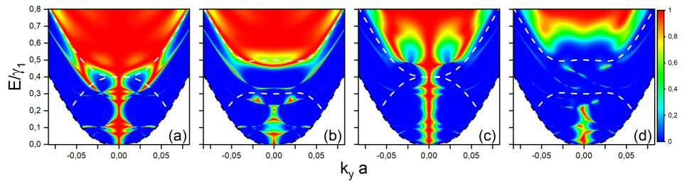
Figure 2: (Color online) Density plot of transmission probability $T^{1}_{1}$, for $\delta_{2}=\delta_{4}=0$ (a,c) and for $\delta_{2}=\delta_{4}=0.2\ \gamma_{1}$ (b,d), versus the incident energy $E$ and the wave vector $ky$ for $V_{2}=V_{4}=0.4\ \gamma_{1}$ (a,b) and for $V_{2}=0.4\ \gamma_{1}$, $V_{4}=0.6\ \gamma_{1}$ (c,d), with $b_{1}=b_{2}=\Delta=10$ nm. The dashed white lines show the band inside the barrier whereas the black lines represent the band outside the barrier.

To determine the transmission and reflection we use the boundary conditions in addition to the current density. We start from the continuity of the spinors at different interfaces to obtain the coefficients in the incident and reflected regions

$$C^{s}_{\text{I}}=\left(\begin{array}[]{cccccc}\delta_{s,1}\\ r^{s}_{1}\\ \delta_{s,2}\\ r^{s}_{2}\\ \delta_{s,3}\\ r^{s}_{3}\\ \end{array}\right),\qquad C^{s}_{\text{V}}=\left(\begin{array}[]{c}t^{s}_{1}\\ 0\\ t^{s}_{2}\\ 0\\ t^{s}_{3}\\ 0\\ \end{array}\right)$$ (22)

which can be coupled via the transfer matrix $M$ as

$$C^{s}_{\text{I}}=MC^{s}_{\text{V}}$$ (23)

resulted from the continuity of spinors at the four interfaces of the double barrier structure (Fig. 1(a)). The remaining relations are given by

$$Q^{\text{I}}M^{\text{I}}(0)C^{\text{I}}=Q^{\text{II}}M^{\text{II}}(0)C^{\text{II}},$$ (24)

$$Q^{\text{II}}M^{\text{II}}(a)C^{\text{II}}=Q^{\text{III}}M^{\text{III}}(a)C^{\text{III}},$$ (25)

$$Q^{\text{III}}M^{\text{III}}(b)C^{\text{III}}=Q^{\text{IV}}M^{\text{IV}}(b)C^{\text{IV}},$$ (26)

$$Q^{\text{IV}}M^{\text{IV}}(c)C^{\text{IV}}=Q^{\text{V}}M^{\text{V}}(d)C^{\text{V}}.$$ (27)

Now solving the above system of equations and taking into account of Eq. (21), one can find the form of $M$. Then we can specify the complex coefficients of the transmission $t^{s}_{i}$ $(i=1,2,3)$ and reflection $r^{s}_{i}$ by using $M$.

To obtain the transmission $T$ and reflection $R$ probabilities, we introduce the current density $\overrightarrow{\mathbf{J}}$ associated to our system. Then, one can show

$$\overrightarrow{\mathbf{J}}=v_{F}\mathbf{\Psi}^{\dagger}\overrightarrow{\alpha}\mathbf{\Psi},$$ (28)

where $\boldsymbol{\alpha}$ is a $6\times 6$ matrix having three Pauli matrices $\sigma_{x}$ in diagonal and the remaining elements are nulls. It is clearly seen that Eq. (28) allows to obtain the incident $\mathbf{J}_{\sf inc}$, transmitted $\mathbf{J}_{\sf tra}$ and reflected $\mathbf{J}_{\sf ref}$ density currents. Consequently, we get

$$T=\frac{|\mathbf{J}_{\sf tra}|}{|\mathbf{J}_{\sf inc}|},\qquad R=\frac{|\mathbf{J}_{\sf ref}|}{|\mathbf{J}_{\sf inc}|}.$$ (29)

By using Eq. (15), we explicitly determine $T$ and $R$

$$T^{s}_{i}=\frac{A^{x}_{i,i}}{A^{x}_{s,s}}|t^{s}_{i}|^{2},\qquad R^{s}_{i}=\frac{A^{x}_{i,i}}{A^{x}_{s,s}}|r^{s}_{i}|^{2},$$ (30)

such that $A^{x}_{i,i}$ and $A^{x}_{s,s}$ are elements of the diagonal matrix $\overrightarrow{\mathbf{A}}=Q^{\dagger}\overrightarrow{\alpha}Q$ consisting of traceless $2\times 2$ blocks where each one corresponds to a propagation mode $s$. These expressions can be explained as follows. Since we have six band, the electrons can be scattered between them and then we need to take into account the change in their velocities. With that, we find nine channels in transmission and reflection corresponding to three modes of propagation $k^{1}$, $k^{2}$ and $k^{3}$ solutions of the cubic Eq. (12).

Fig. 1(c) shows the modes $k^{1}$, $k^{2}$, $k^{3}$ with theirs transmission and reflection probabilities through double barrier structure. For $E<\gamma_{1}$ (low energies ), there is only the mode of propagation $k^{1}$, which gives rise to one transmission $T^{1}_{1}$ and one reflection $R^{1}_{1}$ channel through the two conduction bands touching at zero energy on the both sides of the double barrier. For $E>\gamma_{1}$ (higher energy), the three modes of propagation $k^{1}$, $k^{2}$, $k^{3}$ are present, which leads to nine transmission $T^{1}_{i}$, $T^{2}_{i}$, $T^{3}_{i}$ $(i=1,2,3)$ and reflection $R^{1}_{i}$, $R^{2}_{i}$, $R^{3}_{i}$ channels, through the six conduction bands. For the transmission, there are three non scattered channels denoted by $T^{1}_{1}$, $T^{2}_{2}$, $T^{3}_{3}$ for propagation via $k^{1}$, $k^{2}$, $k^{3}$, respectively, in addition to six scattered channels in which the particle enters via one channel and exits via another one. These will be specified as $T^{1}_{3,2}$, $T^{2}_{3,1}$ and $T^{3}_{2,1}$ for scattering from the $k^{1}$ band to the $k^{3,2}$, from the $k^{2}$ band to the $k^{3,1}$ and from the $k^{3}$ band to the $k^{2,1}$ bands, respectively. Also we will adopt the same definition for the reflection channels, i.e. $R^{1,2,3}_{1,2,3}$. The eighteen channels are schematically depicted in Fig. 1(c). We not that the transmission $T^{1,2,3}_{1,2,3}$ and reflection $R^{1,2,3}_{1,2,3}$ probabilities obeying the following equation

$$\sum_{j=1,2,3}\left(T^{j}_{1,2,3}+R^{j}_{1,2,3}\right)=1.$$ (31)

For example, for the lower band in Fig. 1(c), we have $T^{1}_{1}+R^{1}_{1}+T^{1}_{2}+R^{1}_{2}+T^{1}_{3}+R^{1}_{3}=1.$

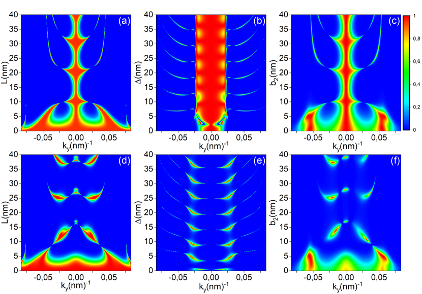
Figure 3: (Color online) (Top row) Density plot of the transmission probability $T^{1}_{1}$ for $V_{2}=V_{4}=0.6\ \gamma_{1}$, $E=\frac{4}{5}\ V_{2}$ and for the gap $\delta_{2}=\delta_{4}=0$ versus (a): $k_{y}$ and the width of the two barriers $(b_{1}=b_{2}=L)$ and $\Delta=10$ nm, (b): $k_{y}$ and $\Delta$ for $b_{1}=b_{2}=10$ nm, (c): $ky$ and $b_{2}$ with $b_{1}=5$ nm and $\Delta=10$ nm. (Bottom row) The same as top row but for the gap $\delta_{2}=\delta_{4}=0.1\ \gamma_{1}$.

Since we have found transmission probabilities, let see how these will effect the conductance of our system. This actually can be obtained through the Landauer-Büttiker formula Blanter336 by summing on all channels to end up with

$$G(E)=G_{0}\frac{L_{y}}{2\pi}\int_{-\infty}^{+\infty}dk_{y}\sum^{3}_{s,n=1}T^{s}_{n}(E,k_{y}),$$ (32)

with the width $L_{y}$ of our system in the $y$-direction and the conductance unit $G_{0}=4e^{2}/h$, the factor $4$ refers to the valley and spin degeneracy in graphene.

The obtained results will be numerically analyzed to discuss the basic features of our system and also make link with other published results. Because of the nature of our system, we do our task by distinguishing two different cases in terms of the band tunneling.

III Band tunneling analysis

We distinguish two interesting cases resulted from our energy spectrum. Indeed, we will separately treat each case and underline their relevant properties. We will compare our results with previous workvanduppen195439 ; Benlakhouy114835 ; vanduppen205427 ; ElMouhafid2017 .

III.1 Tunneling at low energy

Fig. 2 shows a few contour plots of the transmission probability $T^{1}_{1}$ corresponds to the propagation from the channel $k^{1}$ in region I to the channel $k^{5}=k^{1}$ in region V at low energy as a function of the wave vector $k_{y}$ of the incident energy $E$ under suitable conditions of the physical parameters. We address two different cases: (i) the height of the two barriers is the same ($V_{2}=V_{4}$) (symmetric double barrier structure) and (ii) with different height of the two barriers ($V_{2}<V_{4}$) (asymmetric double barrier structure) with and without interlayer potential on both barriers in both cases. Indeed, the case (i) when $V_{2}=V_{4}=0.4\gamma_{1}$ in Fig. 2(a,b) with $\delta_{2}=\delta_{4}=0$ in Fig. 2(a) and $\delta_{2}=\delta_{4}=0.2\gamma_{1}$ in Fig. 2(b) and the the case (ii) when $V_{2}=0.4\gamma_{1}$ and $V_{4}=0.6\gamma_{1}$ in Fig. 2(b,c) with $\delta_{2}=\delta_{4}=0$ in Fig. 2(c) and $\delta_{2}=\delta_{4}=0.2\gamma_{1}$ in Fig. 2(d). It is interesting to note that the Van Duppen et al. results vanduppen195439 can be derived from our analysis by considering (i) and requiring $b=c$ in our double barrier structure. However, the effect of the different structure of the two barriers should appear in the transmission and reflection.

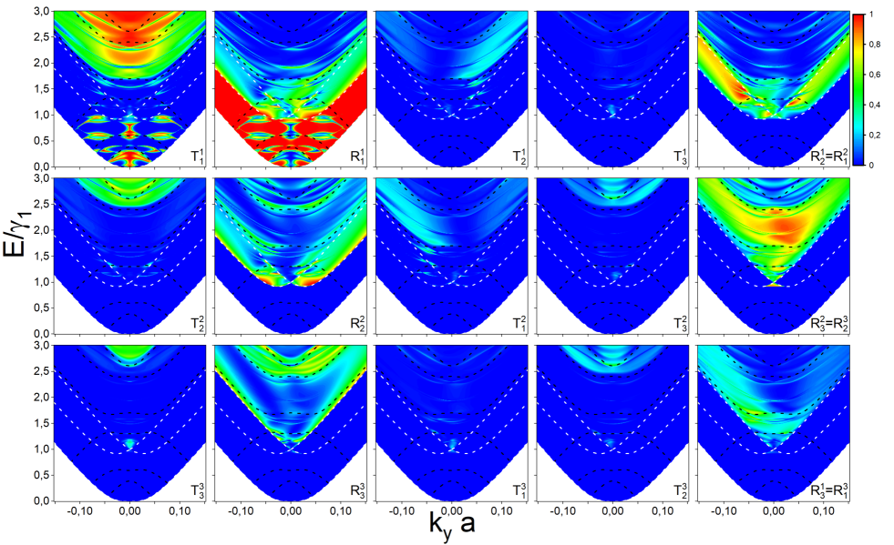
Figure 4: (Color online) Density plot of transmission and reflection probabilities versus $E$ and $k_{y}$ with $V_{2}=V_{4}=1.5\ \gamma_{1}$, $\delta_{2}=\delta_{4}=0.2\ \gamma_{1}$ and $b_{1}=b_{2}=\Delta=10$ nm. The dashed black lines show the band inside the barrier whereas the white lines represent the band outside the barrier. .

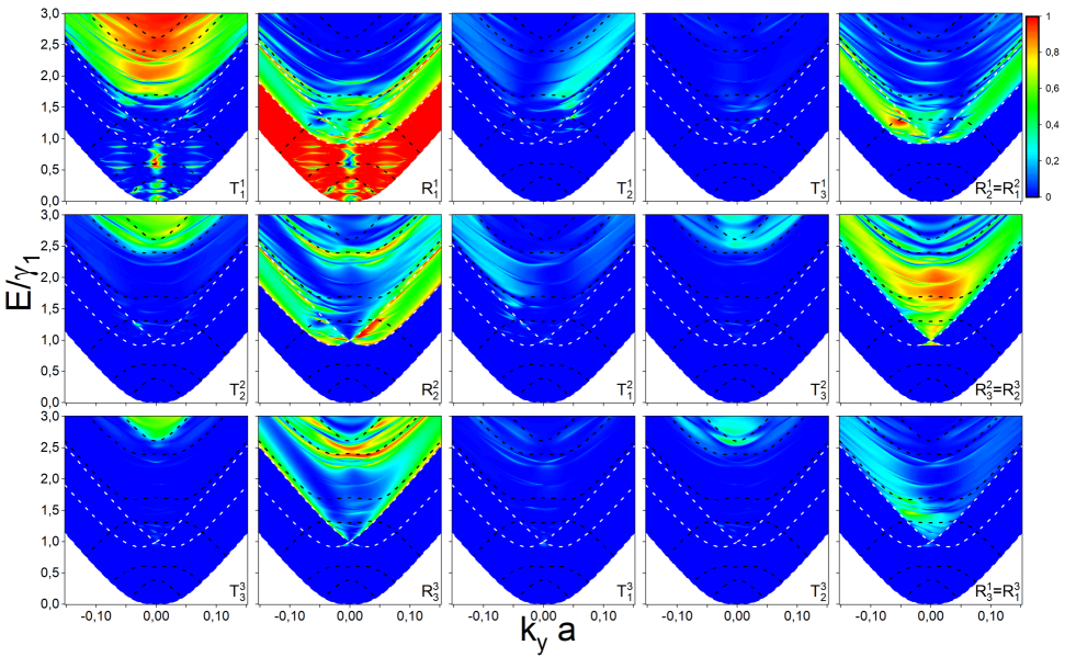
Figure 5: (Color online) The same as Fig. 4 but now for $V_{2}=1.3\gamma_{1}$, $V_{4}=1.5\ \gamma_{1}$.

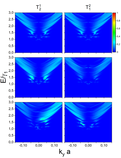
Figure 6: (Color online) Density plot of transmission probabilities $T^{1}_{2}$ (left panel) and $T^{2}_{1}$ (right panel) versus $E$ and $k_{y}$ with $b_{1}=b_{2}=\Delta=10$ nm for $V_{2}=V_{4}=1.5\ \gamma_{1}$ and $\delta_{2}=\delta_{4}=0$ (top row), $V_{2}=1.3\ \gamma_{1}$, $V_{4}=1.5\ \gamma_{1}$ and $\delta_{2}=\delta_{4}=0$ (middle row), $V_{2}=V_{4}=1.5\ \gamma_{1}$, $\delta_{2}=0$ and $\delta_{4}=0.2\gamma_{1}$ (bottom row).

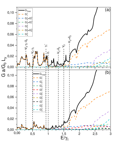
Figure 7: (Color online) Conductance for ABC-TLG versus the incident energy $E$ with $b_{1}=b_{2}=\Delta=10$ nm and $\delta_{2}=\delta_{4}=0.2\gamma_{1}$. (a): $V_{2}=V_{4}=1.5\gamma_{1}$. (b): $V_{2}=1.3\gamma_{1}$, $U_{4}=1.5\gamma_{1}$. The solid lines are for the total conductance and the dashed ones are for the contributions of different propagation channels.

As shown in Fig. 2(a,c), for a normal incidence ($k_{y}=0$) and $\delta_{2}=\delta_{4}=0$ the transmission is unit and becomes independent of energy or the barrier structure (symmetric or asymmetric), which is the same from the single barrier casevanduppen195439 . This is a manifestation of the Klein tunneling that is resulted from the conservation of pseudospin and occurs for rhombohedrally stacked multilayers with an odd number of layersvanduppen195439 . For $\delta_{2}=\delta_{4}=0.2\ \gamma_{1}$, we show $V_{2}=V_{4}=0.4\ \gamma_{1}$ in Fig. 2(b) and $V_{2}=0.4\ \gamma_{1}$, $V_{4}=0.6\ \gamma_{1}$ in Fig. 2(d). For single barrier, in AB-BLGvanduppen205427 ; Benlakhouy114835 and ABC-TLGvanduppen195439 , there are no resonant inside the induced gap in contrary to the double barrier as clearly seen in Fig. 2(b,d). Without $\delta_{2}$, $\delta_{4}$ and for $k_{y}\neq 0$ we still have a full transmission (very narrow resonances), even for $E<V_{j}$, which are symmetric in $k_{y}$. Such resonances get reduced and even disappeared in Fig. 2(b,d) due to the asymmetric structure of double barrier. We notice that the asymmetric structure of double barrier reduces these resonances resulted from the bound electrons in the well between the two barriers, which are similar to those obtained for AB-BLGElMouhafid2017 .

Fig. 3 presents the density plot of the transmission probability as a function of the wave vector $k_{y}$ and the width of two barriers for $V_{2}=V_{4}=0.6\ \gamma_{1}$ and $E=\frac{4}{5}V_{2}$, $\delta_{2}=\delta_{4}=0$ and $\delta_{2}=\delta_{4}=0.1\gamma_{1}$ in top and bottom rows, respectively. For $k_{y}=0$ we have a full transmission regardless of thickness $b_{1}$ and $b_{2}$ of the two barriers or distance $\Delta$ between them. In contrary, with increasing $L$, $\Delta$ and $b_{2}$, the transmission probability dramatically decreases however, some resonances still show up as depicted in Fig. 3(a,b,c). The transmission probability in Fig. 3(b) is completely different compared to Fig. 3(a,c) where the position and number of resonant change. We can see clearly in Fig. 3(b) for a gapless ABC-TLG the existence of a brighter region corresponding to higher transmission probability for a wide range of $k_{y}$ between $\pm 0.025\ \text{nm}^{-1}$ for any values of barrier well $\Delta$. This tells us that the crucial parameter in determining the number of resonant peaks together with theirs positions is the well width $\Delta$ in similar way to the AB-bilayer grapheneElMouhafid2017 .

Notice that at non normal incidence, i.e., $ky\neq 0$ and for $\delta_{2}=\delta_{4}=0$ the transmission still equals unity as a result of the Febry-Pèrot oscillations, independent of width $b_{1}$ or $b_{2}$ or well $\Delta$ between the two barriers which is the same from the single barrier case in AB-BLGvanduppen205427 ; Benlakhouy114835 and ABC-TLGvanduppen195439 .

For $\delta_{2}=\delta_{4}=0.2\ \gamma_{1}$, the density plots in the Fig. 3(bottom row) and for the chosen symmetric barrier show that Klein tunneling is suppressed at normal incidence for some values of barrier width $b1$ or $b2$ and well $\Delta$, there by illustrating some possible reflection even for zero angle of incidence $\phi=\arcsin{(ky/E)}$. We notice that most of the resonances disappeared and splitted due to the band gap in the energy spectrum generated from the induced electric field. A full transmission frequently occur for normal and non normal incidence as $L$, $\Delta$ and $b_{2}$ increases as shown in Fig. 3 for both gap and gapless ABC-TLG.

III.2 Tunneling at high energy

At high energy where all propagation modes are taken into account, the transmission and reflection probabilities as a function of the incident energy $E$ and the wave vector $k_{y}$, corresponding to the modes schematized in Fig. 1(c), are presented in Fig. 4 and in Fig. 5 through symmetric $V_{2}=V_{4}=1.5\gamma_{1}$ and asymmetric $V_{2}=1.3\gamma_{1}$ and $V_{4}=1.5\gamma_{1}$ double barrier structure, respectively, with an interlayer potential difference $\delta_{2}=\delta_{4}=0.2\gamma_{1}$ and width $b_{1}=b_{2}=\Delta=10\ nm$ in both cases. The dashed black lines show the band inside the barrier whereas the white lines represent the band outside the barrier. These lines separate between different regions in the transmission and reflection probabilities, which can be explained by identifying which modes are propagating inside and outside our system in Fig. 1(a). In our double barrier potential we have nine channels of transmission rather than six unlike the case of ABC-TLGvanduppen195439 in one barrier. Specifically, in double barrier structure the symmetry in the scattered transmission $T^{i}_{j}$, with $i\neq j$ and $(i,j)=(1,2,3)$, from band $k^{i}$ to band $k^{j}$ is broken with respect to the normal incidence $k_{y}=0$ and $T^{i}_{j}(\pm k_{y})=T^{j}_{i}(\mp k_{y})$ for $V_{2}=V_{4}$ as shown in Fig. 4 and $T^{i}_{j}\neq T^{j}_{i}$ for $V_{2}\neq V_{4}$ as shown in 5 as in the case of AB-BLG in vanduppen205427 ; Benlakhouy114835 and unlike the case of ABC-TLGvanduppen195439 in one barrier. This can be also understood by pointing out that for the symmetric (asymmetric) structure the particles scattered from top layer to bottom one once moving from left to right in the valley $K$ are equivalent (non equivalent) to particles scattered from bottom layer to top one once moving oppositely in the second valley $K^{\prime}$. However, the element responsible for this asymmetry in transmission is the introduction of an interlayer potential difference $\delta_{2}$ or $\delta_{4}$ or both $\delta_{2}$ and $\delta_{4}$ in the system as shown in addition to Fig. 4 and Fig. 5 in Fig. 6. For $\delta_{2}=\delta_{4}=0$ for symmetric (asymmetric) double barrier structure the symmetry in the scattered transmission $T^{i}_{j}$ still valid and $T^{i}_{j}=T^{j}_{i}$ ($T^{i}_{j}\neq T^{j}_{i}$) as shown in Fig. 6 for $T^{1}_{2}$ and $T^{2}_{1}$. We note that, identically to the transmission probabilities $T^{i}_{j}$ analysis, we can clearly see that the behavior of the reflection probabilities $R^{i}_{j}$ $((i,j)=1,2,3$) is the same in terms of symmetry and asymmetry except that the $R^{i}_{j}(\pm k_{y})$ and $R^{j}_{i}(\pm k_{y})$ are always equals regardless the existence or not of the interlayer potential difference as in one barriervanduppen195439 . The transmissions probabilities $T^{i}_{i}$ ($i=1,2,3$) exhibit a very similar behavior with respect to the normal incidence $k_{y}=0$, which is due to the symmetry of the system unlike the $V1\neq V_{4}$ the $T^{i}_{i}$ are not symmetric and $T^{i}_{i}\neq T^{j}_{j}$ ($i\neq j$). We observe that The barrier heights act by reducing the transmission probabilities. However, theirs effects become more intense inside the gap, which are due to the fact that the available states outside the first barrier are in the same energy zone of the gap on the second barrier.

At normal incidence, and in contrast to the single barrier casevanduppen195439 as shown in Fig. 4 and 5 there are a transmission in $T^{1}_{1}$ different than zero inside the gap in the energy spectrum resulted from the available states in the well between the barriers, which are similar to those obtained for AB-BLGElMouhafid2017 . In addition, Klein tunneling in $T^{1}_{1}$ occur for the range of energy $V_{2}-\gamma_{1}<E<\gamma^{\prime}_{1}$, $E<V_{2}-\gamma_{1}-\delta_{2}$ and $E>V_{2}+\delta_{2}$ for both symmetric and non symmetric barrier where $\gamma_{1}^{\prime}=0.918\gamma_{1}$vanduppen195439 . Outside the previous energy ranges the transmission $T^{1}_{1}$ is nearly zero. For $E<\gamma_{1}$ the transmission probabilities $T^{i}_{j}=0$ $(i\neq j)$ $((i,j)=1,2,3$) and the reflection probabilities $R^{1}_{1}\neq 0$ and $R^{i}_{j}=0$ $(i\neq j)$. It implies that at low energy the propagation from region I to region V is only valid by one channel $k^{1}$, as in the case of the one barrier in AB-BLGvanduppen205427 ; Benlakhouy114835 and ABC-TLGvanduppen195439 . We observe the suppression in transmission due to cloaking effect at non-normal incidencevanduppen195439 ; Rudner156603 , which also exists for some states as a result of the available states in the well.

IV Conductance

The energy dependence of the conductance of ABC-TLG through symmetric and asymmetric double barrier structure is shown in Figs. 7(a) and (b), respectively for different values of the applied gate voltage. The solid lines are the total conductance and the dashed ones are for the contributions of different propagation channels. The resonances that are visible in the transmission probabilities in Figs. 4 and 5 due to the existence of the bound electron states in the well mentioned in the previous section are responsible for the appearance of the peaks in the double barrier conductance. These resonances are more important in Fig. 7(a) for symmetric structure than in Fig. 7(b) for asymmetric structure. Several local maxima and minima are observed which are strongly dependent on the structure of the barrier. It is clearly seen in Figs. 7(a) and (b) that for $E<\gamma_{1}^{\prime}$ once the propagating states become available, the conductance shows an sharply increase to unity in the regime where only one band $T^{1}_{1}$ is available for contributing to the conductance. For $E>\gamma_{1}^{\prime}$ when more bands become possible, additional transmission channels contribute by increasing the conductance to almost perfect one with $G^{1}_{2}=G^{2}_{1}$, $G^{1}_{3}=G^{3}_{1}$ and $G^{2}_{3}=G^{3}_{2}$ in Fig. 7(a) for symmetric structure and unlike in the Fig. 7(b) when $G^{1}_{2}\neq G^{2}_{1}$, $G^{1}_{3}\neq G^{3}_{1}$ and $G^{2}_{3}\neq G^{3}_{2}$ for asymmetric structure.

V Conclusion

We have investigated the tunneling effect of electrons through symmetric and asymmetric double barrier potential in ABC-TLG system. Using the six band model, we have derived the solutions of energy spectrum in all regions composing our system. By matching the eigenspinors at different interfaces, we have determined all possible channels of the transmission and reflection coefficients. Based on the symmetric and asymmetric double barrier structure, we have studied the transmissions by specifying two energy zones $E<\gamma_{1}^{\prime}$ (one propagating mode) and $E>\gamma_{1}^{\prime}$ (three propagating modes) in addition to various values of the barrier heights and widths.

Additionally, we have compared our results with previous work vanduppen195439 (for $E<\gamma_{1}$) and showed that without gap at normal incidence ($k_{y}=0$) for symmetric or asymmetric structure the transmission equals unity independent of energy or width or well between the two barriers or barrier structure as it was the case for a single barriervanduppen195439 . At $k_{y}\neq 0$ we have seen that the transmission shows a sequence of the resonances in the region $E<V_{j}$, which is a consequence of the bounded electrons in the well between two barriers. We have showed that to control the position and the number of these resonances, in both cases $E<\gamma_{1}^{\prime}$ or $E>\gamma_{1}^{\prime}$, it is interesting to use the well width between the tow barriers rather than the thickness of the barriers as obtained in AB-BLGElMouhafid2017 .

It was showed that the asymmetric structure of the double potential barrier reduces the transmission probabilities and removes the sharp resonant peaks as well. Furthermore, the transmission symmetry is prized and the element responsible for this asymmetry is the presence of an interlayer potential difference in region II or in region IV or both II and IV. However, we have observed that the resulting conductance for the double barrier turned into distinctive from that of the single barrier. This distinction manifests itself via the presence of many extra resonances that are related to the bound electron states in the well.

References

- (1) K. S. Novoselov, A. K. Geim, S. V. Morozov, D. Jiang, Y. Zhang, S. V. Dubonos, I. V. Grigorieva, and A. A. Firsov, Science 306, 666 (2004).
- (2) K. S. Novoselov, A. K. Geim, S. V. Morozov, D. Jiang, M. I. Katsnelson, I. V. Grigorieva, S. V. Dubonos, and A. A. Firsov, Nature 438, 197 (2005).
- (3) Y. B. Zhang, Y. W. Tan, H. L. Stormer, and P. Kim, Nature 438, 201 (2005).
- (4) A.K. Geim, and K.S. Novoselov, Nature Materials 6, 183 (2007).
- (5) M. Aoki and H. Amawashi, Solid State Commun. 142, 123 (2007).
- (6) M. S. Dresselhaus and G. Dresselhaus, Advances in Physics 51, 186 (2002).
- (7) M. Koshino and T. Ando, Solid State Commun. 149, 1123 (2009).
- (8) S. H. Jhang, M. F. Craciun, S. Schmidmeier, S. Tokumitsu, S. Russo, M. Yamamoto, Y. Skourski, J. Wosnitza, S. Tarucha, J. Eroms, and C. Strunk, Phys. Rev. B 84, 161408(R) (2011).
- (9) M. Koshino, Phys. Rev. B 81, 125304 (2010).
- (10) C. H. Lui, Z. Q. Li, Z. Y. Chen, P. V. Klimov, L. E. Brus, and T. F. Heinz, Nano Lett. 11, 164 (2011).
- (11) S. Latil and L. Henrard, Phys. Rev. Lett. 97, 036803 (2006).
- (12) E. McCann and M. Koshino, Rep. Prog. Phys. 76, 056503 (2013).
- (13) A. I. Cocemasov, D. L. Nika, and A. A. Balandin, Phys. Rev. B 88, 035428 (2013).
- (14) K. F. Mak, J. Shan, and T. F. Heinz, Phys. Rev. Lett. 104, 176404 (2010).
- (15) F. Guinea, A. H. C. Neto, and N. M. R. Peres, Phys. Rev. B 73, 245426 (2006).
- (16) A. A. Avetisyan, B. Partoens, and F. M. Peeters, Phys. Rev. B 80, 195401 (2009).
- (17) A. A. Avetisyan, B. Partoens, and F. M. Peeters, Phys. Rev. B 81, 115432 (2010).
- (18) C. L. Lu, C. P. Chang, Y. C. Huang, R. B. Chen, and M. L. Lin, Phys. Rev. B, 73, 144427 (2006).
- (19) B. Van Duppen and F. M. Peeters, Europhys. Lett. 102, 27001 (2013).
- (20) Raad Chegel, Synthetic Metals 223, 172 (2017).
- (21) Lei Hao and L. Sheng, Solid State Commun. 149, 1962 (2009).
- (22) Celal Yelgel, J. Phys.: Conf. Ser. 707, 012022 (2016).
- (23) S. Bala Kumar and Jing Guo, Appl. Phys. Lett. 98, 222101 (2011).
- (24) M. I. Katsnelson, K. S. Novoselov, and A. K. Geim, Nat. Phys. 2, 620 (2006).
- (25) M. Ramezani Masir, P. Vasilopoulos, and F. M. Peeters, Phys. Rev. B 82, 115417 (2010).
- (26) S. B. Kumar and J. Guo, Appl. Phys. Lett. 100, 163102 (2012).
- (27) B. Van Duppena and F. M. Peeters, Appl. Phys. Lett. 101, 226101 (2012).
- (28) B. Van Duppen and F.M. Peeters, Physical Review B 87, 205427 (2013).
- (29) B. Van Duppen, S. H. R. Sena, and F. M. Peeters, Phy. Rev. B 87, 195439 (2013).
- (30) J.M. Pereira, P. Vasilopoulos, and F.M. Peeters, Physical Review B 79, 155402 (2009).
- (31) M. Mirzakhani, M. Zarenia, P. Vasilopoulos, and F. M. Peeters, Phys. Rev. B 95, 155434 (2017).
- (32) H. M. Abdullah, A. El Mouhafid, H. Bahlouli and A. Jellal, Mater. Res. Express 4, 025009 (2017).
- (33) N. Benlakhouy, A. El Mouhafid, A. Jellal, Physica E 134, 114835 (2021).
- (34) M. Koshino and E. McCann, Phys. Rev. B 80, 165409 (2009).
- (35) F. Zhang, B. Sahu, H. K. Min, and A. H. MacDonald, Phys. Rev. B 82, 035409 (2010).
- (36) S. H. R. Sena, J. M. Pereira, F. M. Peeters, and G. A. Farias, Phys. Rev. B 84, 205448 (2011).
- (37) K. Zou, F. Zhang, C. Clapp, A. H. MacDonald, and J. Zhu, Nano Lett. 13, 369 (2013).
- (38) J. Jung and A. H. MacDonald, Phys. Rev. B 88, 075408 (2013).
- (39) Salah Uddin and K. S. Chan, Journal of Applied Physics 116, 203704 (2014).
- (40) Marcos G. Menezes, Rodrigo B. Capaz, and Steven G. Louie, Phys. Rev. B 89, 035431 (2014).
- (41) R. Ma, L. Sheng, M. Liu, and D. N. Sheng, Phys. Rev. B 86, 115414 (2012).
- (42) S. Yuan, R. Roldán, and M. I. Katsnelson, Phys. Rev. B 84, 125455 (2011).
- (43) M. G. Menezes, R. B. Capaz, and S. G. Louie, Phys. Rev. B 89, 035431 (2014).
- (44) L. J. Yin, W. X. Wang, Y. Zhang, Y. Y. Ou, H. T. Zhang, C. Y. Shen, and L. He, Phys. Rev. B 95, 081402 (2017).
- (45) Y. Barlas, R. Cote, and M. Rondeau, Phys. Rev. Lett. 109, 126804 (2012).
- (46) R. Côté, M. Rondeau, A. M. Gagnon, and Y. Barlas, Phys. Rev. B 86, 125422 (2012).
- (47) R. Xu, L. J. Yin, J. B. Qiao, K. K. Bai, J. C. Nie, and L. He, Phys. Rev. B 91, 035410 (2015).
- (48) Yun-Peng Wang, Xiang-Guo Li, James N. Fry, and Hai-Ping Cheng, Phys. Rev. B 94, 165428 (2016).
- (49) Kumar, S., Ajay, Indian J Phys 88, 813 (2014).
- (50) M. F. Craciun, S. Russo, M. Yamamoto, J. B. Oostinga, A. F. Morpurgo, and S. Tarucha, Nat. Nanotechnol. 4, 383 (2009).
- (51) C. H. Lui, Z. Li, K. F. Mak, E. Cappelluti, and T. F. Heinz, Nat. Phys. 7, 944 (2011).
- (52) L. C. Campos, A. F. Young, K. Surakitbovorn, K. Watanabe, T. Taniguchi, and P. Jarillo-Herrero, Nat. Commun. 3, 1239 (2012).
- (53) B. Partoens and F. M. Peeters, Phys. Rev. B 75, 193402 (2007).
- (54) F. Zhang, J. Jung, G. A. Fiete, Q. Niu, and A. H. Mac- Donald, Phys. Rev. Lett. 106, 156801 (2011).
- (55) R. Côté and Manuel Barrett, Phys. Rev. B 88, 245445 (2013).
- (56) M. Barbier, P. Vasilopoulos, and F.M. Peeters, Physical Review B 82, 235408 (2010).
- (57) Ya. M. Blanter, and M. Büttiker, Physics Reports 336, (2000).
- (58) N. Gu, M. Rudner, and L. Levitov, Physical Review Letters 107, 156603 (2011).