Abstract

This paper develops a monetary-search model where the money multiplier is endogenously determined. I show that when the central bank pays interest on reserves, the money multiplier and the quantity of the reserve can depend on the nominal interest rate and the interest on reserves. The calibrated model can explain the evolution of the money multiplier and the excess reserve-deposit ratio in the pre-2008 and post-2008 periods. The quantitative analysis suggests that the dramatic changes in the money multiplier after 2008 are driven by the introduction of the interest on reserves with a low nominal interest rate.

JEL Classification Codes: E42, E51
Keywords: Money, Credit, Interest on Reserves, Banking, Monetary Policy

[A] model of the banking system in which currency, reserves, and deposits play distinct roles … seems essential if one wants to consider policies like reserves requirements, interest on deposits, and other measures that affect different components of the money stock differently. Lucas (2000)

1 Introduction

After the Great Recession, many economists have been trying to better understand the substantial changes in the conduct of monetary policy. Most of the literature focuses on the independence of the quantity of reserves from interest rate management in an ample-reserves regime (e.g., Keister, Martin and McAndrews, 2008; Curdia and Woodford, 2011; Bech and Klee, 2011; Kashyap and Stein, 2012; Cochrane, 2014; Ennis, 2018). The rationale is that the interest rate paid on reserves provides a floor for the short-term interest rate that the central bank seeks to control. Then, as the central bank’s target reaches the interest rate on reserves, paying interest on reserves “divorces” money from interest rate management, and the central bank can determine the amount of reserves independently of the interest rate. This implies market rates are equal to or higher than the interest rate on reserves.

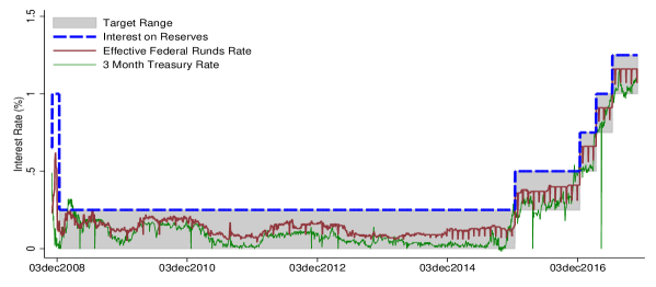
Figure 1: US short-term Interest rates and the target range by the Federal Reserve

However, as Figure 1 shows, since the Federal Reserve introduced the target interest rate range in December 2008 the interest on reserves has been higher than the federal funds rate and has been equal to the upper limit of the target range. Also, the short-term interest rate is closely correlated to the amount of reserves rather than independent. The left panel of Figure 2 plots the excess reserves ratio against the spread between the federal funds rate and the interest on reserves. It shows that the excess reserves ratio and the interest rate spread move in opposite direction. It suggests that, contrary to the previous work, the quantity of reserves is not independent of the central bank’s interest rate management even in the post-2008 period with ample reserves. In addition to that, the right panel of Figure 2 shows that the money multiplier moves together with the interest rate spread, which is just opposite to the excess reserves ratio. The time-series variation in the excess reserve ratio is directly reflected in the M1 money multiplier. This implies that the monetary policy in the post-2008 period is closely related to the banks’ money creation activity, whereas many of monetary models did not pay attention to the money multiplier during last decades. These discrepancies call for a model that better captures for the transmission of monetary policy through the banking system.

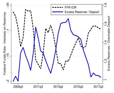
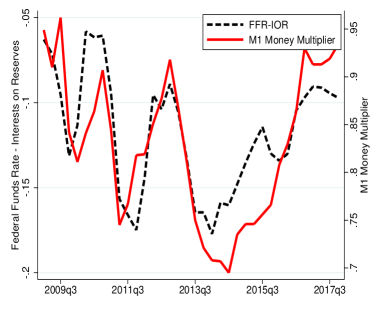
Figure 2: US Excess reserves and M1 multiplier in the post-2008 period

This paper revisits the issue of money creation to understand the role of banking in conducting monetary policy during the pre-2008 period as well as the post-2008 period. To guide the modeling, Section 2 presents a series of empirical facts on money creation and money demand. In contrast to the textbook explanation of the money multiplier, there is no negative relationship between the required reserve ratio and the M1 money multiplier during the period of zero excess reserves. I identify two structural breaks in the money creation process since 1960: (1) one associated with consumer credit, and (2) one associated with interest on reserves. The first structural break in 1992 coincides with a structural break of the deposit component of money demand. A stable long-run money demand relationship, however, is recovered if one accounts for the impact of unsecured credit. The second structural break in 2008 coincides with the Fed’s introduction of the interest on reserves. Banks have been holding excess reserves since then.

These findings suggest that if one wants to study monetary transmission, a desirable monetary model should have the following properties. First, the model should feature the distinct role of the interest on reserves and the nominal interest rate. Second, the model should be able to answer why banks are holding excess reserves now whereas they did not before 2008. Lastly, the model needs to capture the interaction between money and credit.

This paper builds a model based on Lagos and Wright (2005) and Berentsen et al. (2007) of money and banking to understand the monetary transmission under different regimes (e.g., ample-reserves regime, scarce-reserves regime) and identify the factors that changed the regimes from one to another. The bank’s demand for reserves and inside money creation are endogenously determined. The model includes the explicit structure of monetary exchange and the role of financial intermediation. Agents can trade by using cash, claims on deposits (e.g., check or debit card), banknotes, and unsecured credit (e.g., credit card). The bank creates banknotes by making loans, and its lending is constrained by the reserve requirement. The equilibrium falls into one of the following three cases: a scarce-reserves equilibrium, an ample-reserves equilibrium, and a no-banking equilibrium.

In the scarce-reserves equilibrium, the nominal interest rate is sufficiently high. The bank’s lending limit binds. If the central bank lowers the nominal interest rate, the reserve balance increases. The bank creates loans proportional to reserves, which implies the reserve requirement affects the money multiplier. If the central bank pays interest on reserves and sets the nominal interest rate at some moderate level, the bank holds excess reserves. We call this an ample-reserves equilibrium. In the ample-reserves equilibrium, the bank’s lending limit does not bind. The reserve requirement does not change the money multiplier. Instead, the money multiplier is determined by the nominal interest rate and the interest on reserves. Lowering the nominal interest rate increases reserves, but the banks do not create banknotes proportionally, which lowers the money multiplier. A higher interest on reserves decreases the money multiplier since the bank has more incentive to hold reserve and less incentive to create banknotes. The interest on reserves and the nominal interest rate play distinct roles and they jointly determine the quantity of reserves. These are new findings compared with the literature. In both cases, better credit conditions reduce the real balance of inside money and reserves, but not cash, which results in a lower money multiplier. When the nominal interest rate is low enough, there is sufficient outside money to facilitate trade so buyers do not need to deposit their balances in the bank. The bank can not create inside money because it does not hold any reserves. This is called a no-banking equilibrium.

Next I quantify the model to determine the impact of the monetary policy and the introduction of consumer credit on reserves and the money multiplier. The model is parameterized to match pre-2008 US data. Quantitatively, the calibrated model can account for the behavior of money creation before and after 2008. The model-generated series can mimic the historical behavior of the M1 money multiplier, the excess reserves to deposit ratio, and the currency deposit ratio. The welfare analysis shows that lowering the reserve requirement or paying interest on reserves can reduce the welfare cost of inflation. Also, the quantitative analysis identifies the source of changes in the money multiplier and means of payment. The counterfactual analysis shows that the pre-2008 trend of a decreasing money multiplier is driven by an increase in unsecured credit, whereas the post-2008 trend of a decreasing money multiplier is not attributed to the increase in unsecured credit. From the model and data, I provide evidence that suggests the dramatic changes in the money multiplier after 2008 are mainly driven by the Federal Reserve’s monetary policy: the introduction of the interest on reserves with low nominal interest rate.

This paper is organized as follows. Section 2 provides motivating evidence. Section 3 constructs the search-theoretic monetary model of money creation. Section 4 calibrates the model to quantify the theory. Section 5 concludes.

2 Motivating Evidence

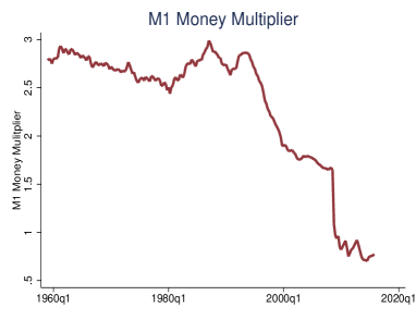
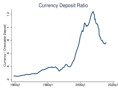
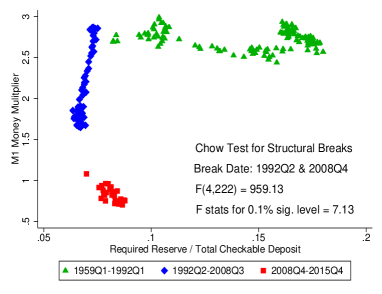
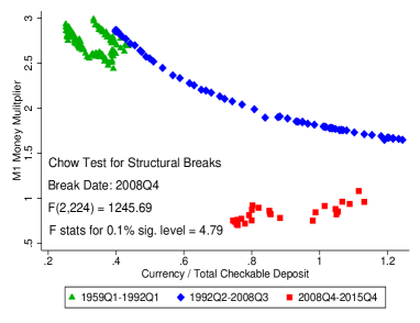
Figure 3: Money multiplier, currency/deposit ratio and required reserve ratio

Chow tests for structural breaks are implemented. The bottom-left panel reports a test statistic with the null hypothesis of no structural breaks in 1992Q2 and 2008Q4 and the bottom-right panel reports a test statistic with the null hypothesis of no structural break in 2008Q4. Sample periods are 1959Q1-2015Q4. Appendix B.1 contains details of the Chow tests.

Whereas the money multiplier decreased drastically since 2008, the decrease in the money multiplier itself is not is a recent phenomenon. The top-left panel of Figure 3 shows that the US M1 money multiplier has been decreasing since 1992. However, the declining trends before and after 2008 are different. As the top-right panel of Figure 3 shows, the decline during 1992-2007 is accompanied by a huge increase in the ratio of currency to deposit, whereas the decline after 2008 is accompanied by a huge drop in the ratio of currency to deposit. The bottom-left panel of Figure 3 reports two structural breaks in the relationship between M1 multiplier and the required reserve ratio: 1992Q3 and 2008Q4.^, It also shows that there is no negative relationship between M1 money multiplier and the required reserve ratio from 1992Q2 to 2008Q3; the excess reserve ratio had been zero until 2008, which suggests that the required reserve ratio does not drive the money multiplier.

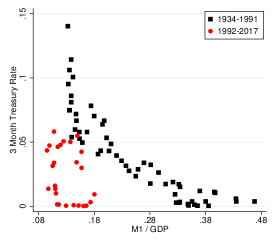
Figure 4: US Money demand for M1 and its components

To offer a better picture of what had happened at the structural break of 1992, Figure 4 plots the ratio of M1 to GDP and the ratio of M1’s components to GDP against the 3 month Treasury Bill rate. There is a breakdown in M1 in 1992 that coincides with the structural break in Figure 3. As pointed out by Lucas and Nicolini (2015), this is due to the breakdown of the deposit component, not the currency component. My hypothesis is that the increased availability of consumer credit crowded out deposit but not cash, which implies that once one accounts for the substitution effect of the newly available consumer credit, there should still be a negative relationship between the real money balance and the interest rate.

Following Cagan (1956), and Ireland (2009), I relate the natural logarithm of $m$, the ratio of money balances to income, to the short-term nominal interest rate, denoted by $r$. I also regress $r$ on the natural logarithm of $d$, the ratio of deposit balances to income.

$$ln(m_{t})=\beta_{0}+\beta_{1}r_{t}+\epsilon_{t},\quad ln(d_{t})=\beta_{0}+\beta_{1}r_{t}+\epsilon_{t}$$

In addition to the above specifications, to capture the impact of the improved availability of consumer credit that can substitute the deposit, I add a logarithm of $uc$, the ratio of unsecured credit to income as another regressor as follows.

$$ln(m_{t})=\beta_{0}+\beta_{1}r_{t}+\beta_{2}ln(uc_{t})+\epsilon_{t},\quad ln(d_{t})=\beta_{0}+\beta_{1}r_{t}+\beta_{2}ln(uc_{t})+\epsilon_{t}$$

Table 1: Cointegration regressions and tests

Dependent Variable:	$ln(m_{t})$		$ln(d_{t})$
	OLS	CCR	OLS	CCR
	(1)	(2)	(3)	(4)
$r_{t}$	$0.016^{***}$	$-0.027^{***}$	$0.049^{***}$	$-0.053^{***}$
	(0.004)	(0.004)	(0.009)	(0.009)
$ln(uc_{t})$		$-0.279^{***}$		$-0.574^{***}$
		(0.033)		(0.040)
$adjR^{2}$	0.109	0.970	0.229	0.962
$N$	112	112	112	112
Johansen $r=0$	15.004	41.744	14.934	49.174
5% Critial Value for $r=0$	15.41	29.68	15.41	29.68
1% Critial Value for $r=0$	20.04	35.65	20.04	35.65
Johansen $r=1$	0.027	12.163	0.26	14.319
5% Critial Value for $r=1$	3.76	15.41	3.76	15.41
1% Critial Value for $r=1$	6.65	20.04	6.65	20.04

Notes: Columns (1) and (3) report OLS estimates and columns (2) and (4) report the canonical cointegrating regression (CCR) estimates. First-stage long-run variance estimation for CCR is based on Bartlett kernel and lag 1. For (1) and (2) Newey-West standard errors with lag 1 are reported in parentheses. Intercepts are included but not reported. ***, **, and * denote significance at the 1, 5, and 10 percent levels, respectively. Johansen cointegration test results are reported in columns (1)-(4). Appendix B.2 contains unit root tests for each series. The data are quarterly from 1980Q1 to 2007Q4.

I focus on the post-1980 period, until the arrival of the Great Recession. In Table 1, columns (1) and (3) report the estimates without unsecured credit, and columns (2) and (4) report the estimates with unsecured credit. The Johansen tests in columns (1) and (3) fail to reject the null hypothesis of no cointegration, which confirms the apparent breakdowns from Figure 4, and ordinary least squares (OLS) estimates from columns (1) and (3) both report positive coefficients on $r_{t}$ that contradict the conventional notion of money demand: the stable downward-sloping relationship between real balances and interest rates. In columns (2) and (4), however, the Johansen tests reject their null of no cointegration at a 99 percent confidence level, suggesting there exists a stable relationship between real money balances, interest rates, and real balances of unsecured credit. To estimate the cointegration relationship, I implement the canonical cointegrating regression, proposed by Park (1992), in columns (2) and (4). The estimated coefficients on $r_{t}$ and $ln(uc_{t})$ both are negative and significantly different from zero. Thus, using the cointegrating regressions and tests, I document the evidence that once one accounts for the substitution effect of consumer credit, there still exists a stable negative relationship between real money balances and the interest rates. This substitution effect is a potential explanation for the decline of the money multiplier during 1992Q2-2008Q3.

Figure 5: Excess reserves ratio

The second structural break at 2008Q3, which can be detected from the bottom-right panel of Figure 3 as well as the bottom-left panel, coincides with the Fed’s introduction of the interest on reserves. As Nakamura (2018) points out, the amount of reserves had skyrocketed before interest rates hit zero and its dramatic increase was simultaneous with the Fed’s introduction of the interest on reserves.

To interpret the observed patterns from data, in the following section I develop a model that can incorporate the evolution of the money creation process.

3 Model

The model constructed here extends the standard monetary search model (Lagos and Wright, 2005) by introducing fractional reserve banking and unsecured credit. Time is discrete and two markets convene sequentially in each time period: (1) a frictionless centralized market (CM, hereafter), where agents work, consume, and adjust their balances, following after (2) a decentralized market (DM, hereafter), where buyers and sellers meet and trade bilaterally. The DM trade features imperfect record-keeping and limited commitment. Due to these two frictions, some means of payment are needed in DM trades. Below I describe the economic agents in this economy and the different types of DM meetings.

Buyers and Sellers The economy consists of a unit mass of buyers and a unit mass of sellers who discount their utility each period by $\beta$. The preferences of buyers and sellers for each period are

$$\mathcal{U}^{b}=U(X)-H+u(q)\quad\text{ and }\quad\mathcal{U}^{s}=U(X)-H-c(q),$$

where $X$ is the CM consumption, $H$ is the CM disutility from production, and $q$ is the DM consumption. As standard, assume $U^{\prime}$, $u^{\prime}$, $c^{\prime}>0$, $U^{\prime\prime}$, $u^{\prime\prime}<0$, $c^{\prime\prime}\geq 0$, and $u(0)=c(0)=0$. Consumption goods are perishable. One unit of $H$ produces one unit of $X$ in the CM. The efficient consumption in the CM and DM is denoted by $X^{*}$ and $q^{*}$, respectively, which solve $U^{\prime}(X^{*})=1$ and $u^{\prime}(q^{*})=c^{\prime}(q^{*})$, respectively.

The Bank There are measure $n$ of active banks that is endogenously determined by the free entry condition in the equilibrium. In the CM, the banks accept deposit and decide how much to deposit at the central bank as reserves and how many banknotes to issue. Managing a deposit payment facility incurs a cost. The cost is represented by a cost function $\gamma(\tilde{d})$, where $\tilde{d}$ is the amount of deposit in real terms, $\gamma^{\prime},\gamma^{\prime\prime}>0$, and $\gamma(0)=\gamma^{\prime}(0)=0$. The reserve earns a nominal interest rate of $i_{r}$. The bank extends loans by issuing banknotes. The loans are paid back with interest rate $i_{\ell}$. Enforcing repayment is costly. The cost function is described by $\eta(\tilde{\ell})$, where $\tilde{\ell}$ is the loan in real terms, $\eta^{\prime},\eta^{\prime\prime}>0$, and $\eta(0)=\eta^{\prime}(0)=0$. The bank’s lending is constrained by the reserve requirement, i.e., the bank cannot lend more than $(1-\chi)\tilde{r}/\chi$, where $\chi$ is the reserve requirement and $\tilde{r}$ is the real balance of reserves.

Types of DM meetings There are three types of DM meetings. In DM1, there is no record-keeping device, and the seller can only recognize cash. In DM2, the seller can recognize cash, the claims on bank accounts, and private banknotes. So she accepts cash, deposit receipts and banknotes. In DM3, in addition to the means of payment accepted in DM2, the buyer can trade using unsecured credit with credit limit $\bar{\delta}$ as the trading is monitored imperfectly. The probability of joining a type $j$ meeting is $\sigma_{j}$. The agents get to know which type of meeting they will be going to in the preceding CM.

The Central Bank The central bank controls the base money supply $M$ in the CM. Let $\mu$ denote the base money growth rate. Then the changes in the real balance of base money can be written as

$$\mu M=M^{+}-M,$$

where $x^{+}$ is the value of (any variable) $x$ in the next period. The base money is held in two ways: (1) $C$ as currency in circulation, i.e., outside money held by agents; (2) $R$ as reserves held by a representative bank. Thus,

$$M=C+R.$$

The central bank can control the base money supply in two ways. First, it can conduct a lump-sum transfer or collect a lump-sum tax in the CM. Second, it can increase the money supply by paying interest on reserves, $i_{r}$. Let $T$ represents a lump-sum transfer (or tax if it is negative). The central bank’s constraint is

$$\mu\phi M=\phi(M^{+}-M)=T+i_{r}\phi R,$$

where $\phi$ is the price of money in terms of the CM consumption good.

3.1 The CM Problem

Buyers’ Decisions At the beginning of the CM, each buyer’s subsequent DM meeting type is realized. Therefore, the buyers’ CM problem depends on their DM meeting type. Let $W^{B}_{j}(m,d,b,\ell,\delta)$ denote the CM value function where $j$ is the type of the following DM meeting, $m$ is the cash holding, $d$ is the deposit balance, $b$ is the private banknote holding, $\ell$ is the loan borrowed from the bank during the last CM period, and $\delta$ is the unsecured debt owed to the seller from the previous DM. All the state variables are in unit of the current CM consumption good. Let $\tau$ denote the lump-sum transfer (or tax if it is negative) to the buyer in the CM. Now, consider the value of the CM. For an agent who is going to a type $j$ DM meeting, the CM problem is

$$\begin{split}W^{B}_{j}(m,d,b,\ell,\delta)&=\max_{\begin{subarray}{c}X,H,\hat{m}_{j},\hat{d}_{j},\hat{b}_{j},\hat{\ell}_{j}\end{subarray}}U(X)-H+\beta V^{B}_{j}(\hat{m}_{j},\hat{d}_{j},\hat{b}_{j},\hat{\ell}_{j})\\ \text{ s.t. }(1+\pi)\hat{m}_{j}+(1+\pi)\hat{d}_{j}+X&=m+(1+i_{d})d+b-(1+i_{\ell})\ell-\delta+H+\tau\\ \hat{b}_{j}&=\hat{\ell}_{j},\end{split}$$ (1)

where $\hat{m}_{j}$, $\hat{d}_{j}$, $\hat{b}_{j}$ and $\hat{\ell}_{j}$ are the cash holding, deposit balance, private banknote balance, and debt balance, respectively, carried to the next DM. The first-order conditions (FOCs) are $U^{\prime}(X)=1$ and

$$-(1+\pi)+\beta\partial V^{B}_{j}(\hat{m}_{j},\hat{d}_{j},\hat{b}_{j},\hat{\ell}_{j})/\partial\hat{m}_{j}\leq 0, =\text{ if }\hat{m}_{j}>0$$ (2)

$$-(1+\pi)+\beta\partial V^{B}_{j}(\hat{m}_{j},\hat{d}_{j},\hat{b}_{j},\hat{\ell}_{j})/\partial\hat{d}_{j}\leq 0, =\text{ if }\hat{d}_{j}>0$$ (3)

$$\beta\partial V^{B}_{j}(\hat{m}_{j},\hat{d}_{j},\hat{b}_{j},\hat{\ell}_{j})/\partial\hat{b}_{j}+\beta\partial V^{B}_{j}(\hat{m}_{j},\hat{d}_{j},\hat{b}_{j},\hat{\ell}_{j})/\partial\hat{\ell}_{j}\leq 0, =\text{ if }\hat{\ell}_{j}>0.$$ (4)

The first term on the left-hand side (LHS) of equation (2) is the marginal cost of acquiring cash. The second term is the discounted marginal value of carrying cash to the following DM. Therefore, the choice of $\hat{m}_{j}>0$ equates the marginal cost and the marginal return on cash. A similar interpretation applies to equation (3) for the decision on deposit. For equation (4), the first term on the LHS captures the discounted marginal value of carrying privately issued banknotes from the CM to the following DM, and the second term captures the discounted marginal cost of getting a bank loan. The envelope conditions for $W^{B}_{j}(m,d,b,\ell,\delta)$ are

$$\frac{\partial W^{B}_{j}}{\partial m}=1,\quad\frac{\partial W^{B}_{j}}{\partial d}=1+i_{d},\quad\frac{\partial W^{B}_{j}}{\partial b}=1,\quad\frac{\partial W^{B}_{j}}{\partial\ell}=-(1+i_{\ell}),\quad\frac{\partial W^{B}_{j}}{\partial\delta}=1$$

for all $j=1,2,3$, which implies $W^{B}_{j}(m,d,b,\ell,\delta)$ is linear. This linearity allows us to write

$$W^{B}_{j}(m,d,b,\ell,\delta)=m+(1+i_{d})d+b-\delta-(1+i_{\ell})\ell+W^{B}_{j}(0,0,0,0,0).$$

Let $W^{B}(m,d,b,\ell,\delta)$ be the buyers’ expected value function before the CM at period $t$ opens, i.e., before their subsequent DM meeting type is realized. Then one can write the buyer’s expected value function in the CM as $W^{B}(m,d,b,\ell,\delta)=\sum\sigma_{j}W^{B}_{j}(m,d,b,\ell,\delta)$.

Sellers’ Decisions A seller enters the CM with cash, $m$, deposits, $d$, private banknotes, $b$, and unsecured credit $\delta$ that a buyer owes to the seller from the previous DM. The seller does not borrow from the bank as long as $i_{\ell}>0$. Let $W^{S}_{j}(m,d,b,0,\delta)$ be the sellers’ value function in the CM at period $t$. It can be written as follows:

$$\begin{split}W^{S}_{j}(m,d,b,0,\delta)&=\max_{X,H,\hat{m}_{j},\hat{d}_{j},\hat{b}_{j},\hat{\ell}_{j}}U(X)-H+\beta V^{S}_{j}(\hat{m}_{j},\hat{d}_{j},\hat{b}_{j},\hat{\ell}_{j})\\ \text{ s.t. }(1+\pi)\hat{m}_{j}+(1+\pi)\hat{d}_{j}+X&=m+(1+i_{d})d+b+\delta+H+\tau\\ \hat{b}_{j}&=\hat{\ell}_{j}\end{split}$$ (5)

As we will see below, the DM terms of trade does not depend on the seller’s portfolio, there is no incentive for the sellers to carry any liquidity to the next DM as the cost of holding liquidity is positive. The envelope conditions are

$$\frac{\partial W^{S}_{j}}{\partial m}=1,\quad\frac{\partial W^{S}_{j}}{\partial d}=1+i_{d},\quad\frac{\partial W^{S}_{j}}{\partial b}=1,\quad\frac{\partial W^{B}_{j}}{\partial\delta}=1$$

for all $j\in\{1,2,3\}$, which implies $W^{S}_{j}(m,d,b,0,\delta)$ is linear. By linearity, the CM value function can be written as

$$W^{S}_{j}(m,d,b,0,\delta)=m+(1+i_{d})+b+\delta+W^{S}_{j}(0,0,0,0,0).$$

3.2 The DM Problem

In the DM, the buyer and seller trade bilaterally. Let $q_{j}$ and $p_{j}$ be the DM consumption and payment in a type-$j$ DM meeting. The bilateral trade is characterized by $(p_{j},q_{j})$. This trade is subject to $p_{j}\leq z_{j}$ where $z_{j}$ is the total liquidity of the buyer in a type-$j$ meeting. The liquidity position for each type of buyer is

$$z_{1} =m_{1}$$ (6)

$$z_{2} =m_{2}+d_{2}(1+i_{d})+b_{2}$$ (7)

$$z_{3} =m_{3}+d_{3}(1+i_{d})+b_{3}+\bar{\delta}.$$ (8)

The DM terms of trade is determined by Kalai (1977) proportional bargaining. Kalai bargaining solves the following problem:

$$\max u(q)-p\quad\textit{s.t}\quad u(q)-p=\theta\left[u(q)-c(q)\right]$$

where $\theta\in[0,1]$ denotes the buyers’ bargaining power. The payment, $p$, is a function of DM consumption, $q$. This can be expressed as $p=v(q)=(1-\theta)u(q)+\theta c(q)$. Define liquidity premium, $\lambda(q)$, as follows:

$$\lambda(q)=\frac{u^{\prime}(q)}{v^{\prime}(q)}-1=\frac{\theta[u^{\prime}(q)-c^{\prime}(q)]}{(1-\theta)u^{\prime}(q)+\theta c^{\prime}(q)}$$

where $\lambda(q)>0$ for $q<q^{*}$ and $\lambda(q^{*})=0$ with $\lambda^{\prime}(q)<0$ for $q\in[0,q^{*})$. When $z_{j}\geq p^{*}$, the buyer has sufficient liquidity to purchase efficient DM output $q^{*}$. In this case, the payment to the seller is $p^{*}=v(q^{*})$.

By the linearity of $W^{B}_{j}$, we can write a DM value function for a buyer in a type-$j$ meeting as follows:

$$V^{B}_{j}(m_{j},d_{j},b_{j},\ell_{j})=u(q_{j})-p_{j}+W^{B}(m_{j},d_{j},b_{j},\ell_{j},0)\quad$$ (9)

where $p_{j}\leq z_{j}$. The third term on the right-hand side (RHS) is the continuation value when there is no trade. The rest of the RHS is the surplus from the DM trade. DM payments are constrained by $p_{j}\leq z_{j}$. With $v(q_{j})=p_{j}$ and $z_{j}\leq p^{*}$, differentiating $V^{B}_{j}$ and substituting its derivatives into the FOCs from the CM problem yields

$$-(1+\pi)+\beta\big{[}1+\lambda(q_{1})\big{]} =0$$ (10)

$$-(1+\pi)+(1+i_{d})\beta \leq 0,=\text{ if }d_{1}>0$$ (11)

$$-i_{\ell} \leq 0,=\text{ if }\ell_{1}>0$$ (12)

$$-(1+\pi)+\beta\big{[}1+\lambda(q_{i})\big{]} \leq 0,=\text{ if }m_{j}>0\text{ for }j=2,3$$ (13)

$$-(1+\pi)+(1+i_{d})\beta\big{[}1+\lambda(q_{i})\big{]} \leq 0,=\text{ if }d_{j}>0\text{ for }j=2,3$$ (14)

$$-i_{\ell}+\lambda(q_{i}) \leq 0,=\text{ if }l_{j}>0\text{ for }j=2,3,$$ (15)

where $q_{j}=\min\{q^{*},v^{-1}(z_{j})\}$ and $\lambda(q^{*})=0$.

Similarly, the sellers’ DM value function is

$$V^{S}_{j}(m_{j},d_{j},b_{j},\ell_{j})=p_{j}-c(q_{j})+W^{S}_{j}(m_{j},d_{j},b_{j},\ell_{j},0).$$

3.3 The Bank’s Problem

A bank maximizes its profit subject to the lending constraint.

$$\max_{\tilde{r},\tilde{d},\tilde{\ell}}\quad i_{r}\tilde{r}-i_{d}\tilde{d}-\gamma(\tilde{d})+i_{\ell}\tilde{\ell}-\eta(\tilde{\ell})$$ (16)

s.t. $$\tilde{\ell}\leq\bar{\ell}\equiv\frac{1-\chi}{\chi}\tilde{r}$$ (17)

$$\tilde{r}\leq\tilde{d}$$ (18)

Let $\lambda_{L}$ denote the Lagrange multiplier for the lending constraint. It is straightforward to show $\tilde{r}=\tilde{d}$. The FOCs for the bank’s problem can be written as

$$0=i_{r}-i_{d}-\gamma^{\prime}(\tilde{r})+\lambda_{L}\left(\frac{1-\chi}{\chi}\right)$$ (19)

$$0=i_{\ell}-\eta^{\prime}(\tilde{\ell})-\lambda_{L}.$$ (20)

The bank’s ex post profit equals to the entry cost, $k$

$$(i_{r}-i_{d})\tilde{r}+i_{\ell}\tilde{\ell}-\gamma\left(\tilde{r}\right)-\eta(\tilde{\ell})=k.$$ (21)

Suppose there are active banks. Consider two cases. In the first case, the bank’s lending constraint is binding, i.e., $\lambda_{L}>0$. In the second case, the bank’s lending constraint is loose, i.e., $\lambda_{L}=0$. We call the first case a scarce-reserves case, and the second an ample-reserves case.

The Scarce-Reserves Case The bank does not have enough reserves. It needs to acquire reserves to make more loans, which implies a binding constraint. With $\lambda_{L}>0$, the bank’s FOCs (19) and (20) give

$$0=i_{r}-i_{d}-\gamma^{\prime}(\tilde{r})+\Bigg{[}i_{\ell}-\eta^{\prime}(\tilde{\ell})\Bigg{]}\frac{1-\chi}{\chi}.$$ (22)

The Ample-Reserves Case The bank has sufficient reserves. Its lending constraint does not bind. Then the two FOCs for the bank’s problem are

$$0=i_{r}-i_{d}-\gamma^{\prime}(\tilde{r})$$ (23)

$$0=i_{\ell}-\eta^{\prime}(\tilde{\ell}).$$ (24)

The bank’s unconstrained optimal lending, $\ell^{*}$, satisfies

$$i_{\ell}=\eta^{\prime}(\ell^{*})$$

and increases as $i_{\ell}$ rises.

3.4 Stationary Equilibrium

I focus on a symmetric stationary monetary equilibrium in which the same type of agents make the same decisions and the real balances are constant over time. Given that $\phi/\phi^{+}=M^{+}/M=C^{+}/C=1+\mu$, the net inflation rate, $\pi$, is equal to the currency growth rate, $\mu$, in the stationary monetary equilibrium. By the Fisher equation, $1+i=(1+\mu)/\beta$. The market clearing conditions are

$$\sigma_{2}\ell_{2}+\sigma_{3}\ell_{3}=n\tilde{\ell} =\ell$$ (25)

$$\sigma_{2}d_{2}+\sigma_{3}d_{3}=n\tilde{r}=r =\phi R$$ (26)

$$\sigma_{1}m_{1}+\sigma_{2}m_{2}+\sigma_{3}m_{3}=m =\phi C,$$ (27)

where $M=C+R$. Note that $i\geq 0$, i.e., $\mu\geq\beta-1$ is necessary for the existence of equilibrium. Define the stationary equilibrium as follows:

Definition 1 (Stationary Equilibrium).

Given monetary policy, $i$, $i_{r}$, and $\chi$ and credit limit $\bar{\delta}$, a stationary monetary equilibrium consists of real balances $(m_{j},d_{j},\ell_{j})_{j=1}^{3},$ allocation $(q_{1},q_{2},q_{3},X),$ the measure of banks $n$, and prices $(i_{\ell},i_{d})$, such that

1. $(i_{d},i_{\ell},q_{1},q_{2},q_{3})$ solves $(\ref{eq:agent_ps})$-$(\ref{eq:agent_pe})$ and $(\ref{eq:bank_foc1})$-$(\ref{eq:bank_entry})$ with $q_{j}=\min\{q^{*},v^{-1}(z_{j})\}$, where $z_{1}=m_{1}$, $z_{2}=m_{2}+(1+i_{d})d_{2}+\ell_{2}$, and $z_{3}=m_{3}+(1+i_{d})d_{3}+\ell_{3}+\bar{\delta}$.

2. The bank lending $\tilde{\ell}=\min(\bar{\ell},\ell^{*})$, where $\bar{\ell}=(1-\chi)\tilde{r}/\chi$ and $\ell^{*}$ solves $i_{\ell}=\eta^{\prime}(\ell^{*})$

3. Asset markets clear $(\ref{eq:clear21})$-$(\ref{eq:clear22})$.

Given Definition 1, there are three types of equilibria, which are defined as follows:

Definition 2.

In a no-banking equilibrium, $\bar{\ell}=r=n=0$. In an ample-reserves equilibrium, $\bar{\ell}>\ell^{*}\geq 0$. In a scarce-reserves equilibrium, $\ell^{*}\geq\bar{\ell}>0$.

In the no-banking equilibrium, the deposit interest rate is zero, $i_{d}=0$ and there is no active bank. Because the return to holding deposits is dominated or equal to the return to holding currency, agents do not have any incentive to deposit their balances. With zero reserve, the lending limit is zero. Therefore, in this equilibrium, agents only use cash for DM trading. All agents hold the same balance of cash and consume the same amount of consumption goods.

$$i=L(m_{j})\text{ for }j=1,2$$ (28)

and $m_{3}=\max\{0,L^{-1}(i)-\bar{\delta}\}$. In this equilibrium, it is straightforward to see that DM consumption is efficient when $i=0$, i.e. the Friedman rule applies. In the ample-reserves equilibrium, each bank holds sufficient reserves to lend $\ell^{*}$, i.e., $\ell^{*}<\bar{\ell}=(1-\chi)\tilde{r}/\chi$, where $\tilde{r}$ represents the equilibrium reserve balance of each bank. Thus, the unconstrained optimal lending is less than the lending limit. Given $i$ and $i_{r}$, $(\tilde{r},\tilde{\ell})$ solves

$$\left\{1+\eta^{\prime}(\tilde{\ell})\right\}[1+i_{r}-\gamma^{\prime}(\tilde{r})]=1+i,\quad\gamma^{\prime}(\tilde{r})\tilde{r}-\gamma(\tilde{r})+\eta^{\prime}(\tilde{\ell})\tilde{\ell}-\eta(\tilde{\ell})=k.$$

In the scarce-reserves equilibrium, however, the lending limit is lower than the bank’s unconstrained optimal lending. Therefore, the lending constraint (17) binds, i.e., $\ell^{*}>\tilde{\ell}=\bar{\ell}=(1-\chi)\tilde{r}/\chi$. Given $i_{\ell}$ and $i_{d}$, the equilibrium real balance of reserves satisfies

$$r=\begin{dcases}\frac{(\sigma_{2}+\sigma_{3})\chi}{1+i_{d}\chi}L^{-1}(i_{\ell})-\frac{\sigma_{3}\bar{\delta}\chi}{1+i_{d}\chi}&\text{if }\hat{\delta}>\bar{\delta}\\ \frac{\sigma_{2}\chi}{1+i_{d}\chi}L^{-1}(i_{\ell})&\text{if }\hat{\delta}\leq\bar{\delta}\end{dcases}$$ (29)

where $\hat{\delta}=L^{-1}(i_{\ell})$.

For each type of equilibrium, the following results are proved in Appendix A.

Proposition 1.

(i) In the ample-reserves and scarce-reserves equilibrium, $\partial i_{d}/\partial i>0$, $\partial i_{\ell}/\partial i>0$, $\partial i_{d}/\partial i_{r}>0$, and $\partial i_{\ell}/\partial i_{r}<0$. (ii) In the no-banking equilibrium, $\partial i_{d}/\partial i=\partial i_{d}/\partial i_{r}=\partial i_{\ell}/\partial i=\partial i_{\ell}/\partial i_{r}=0.$

Proposition 1 tells us that as long as the measure of banking is positive, the monetary policy rates pass through the deposit rate and lending rate. The deposit rate is strictly increasing in the nominal interest rate and the interests on reserves. The lending rate is strictly increasing in the nominal interest rate but is strictly decreasing in interest on reserves. I also establish conditions for the determination of equilibrium types.

Figure 6: Monetary equilibrium regions in $(i,i_{r})$ space

Proposition 2.

Given $(i_{r},\chi)$: (i) $\exists!$ ample-reserves equilibrium if and only if $i_{r}>\gamma^{\prime}(\hat{r})$ and $i\in(\underline{i},\bar{i})$; (ii) $\exists!$ scarce-reserves equilibrium if and only if either $i>\hat{i}$ and $i_{r}<\gamma^{\prime}(\hat{r})$ or $i>\bar{i}$ and $i_{r}>\gamma^{\prime}(\hat{r})$; (iii) $\exists!$ no banking equilibrium if and only if either $i\in[0,\hat{i})$ and $i_{r}<\gamma^{\prime}(\hat{r})$, or $i\in[0,\underline{i})$ and $i_{r}>\gamma^{\prime}(\underline{r})$; and the thresholds satisfy

$$\hat{i}=\frac{\chi}{1-\chi}[\gamma^{\prime}(\hat{r})-i_{r}]+\eta^{\prime}\left(\frac{1-\chi}{\chi}\hat{r}\right),\quad\bar{i}=[1+i_{r}-\gamma^{\prime}(\hat{r})]\left[1+\eta^{\prime}\left(\frac{1-\chi}{\chi}\hat{r}\right)\right]-1$$

and $\underline{i}=i_{r}-\gamma^{\prime}(\underline{r})$, where $\hat{r}$ solves $\gamma^{\prime}(\hat{r})\hat{r}-\gamma(\hat{r})+\eta^{\prime}\left(\frac{1-\chi}{\chi}\hat{r}\right)\frac{1-\chi}{\chi}\hat{r}-\eta\left(\frac{1-\chi}{\chi}\hat{r}\right)=k$ and $\underline{r}$ solves $\gamma^{\prime}(\underline{r})\underline{r}-\gamma(\underline{r})=k$.

Banks hold excess reserves when the central bank pays sufficiently high interest on reserves with the nominal interest rate at some moderate level. To see the intuition consider the case in which the bank holds reserves. The reserve requirement and the reserve balances determine the lending limit. Due to monotone pass-through from the nominal interest rate to the bank’s lending rate, the bank’s unconstrained optimal lending $\ell^{*}$ is increasing in the nominal interest rate. There exists a threshold of the nominal interest rate below which the lending limit is lower than the bank’s unconstrained lending (scarce-reserves), and above which the lending limit is higher than the bank’s unconstrained lending (ample-reserves). In other words, there is a critical value $\bar{i}$ that satisfies $\ell^{*}=\bar{\ell}=(1-\chi)\tilde{r}/\chi$.

However, when the equilibrium deposit rate is zero, agents have no incentive to deposit their balance in the bank, implying the no-banking equilibrium. As shown in Proposition 1, the deposit rate is monotone in the nominal interest rate and the deposit rate could be zero given some nominal interest rate. There exists a threshold $\hat{i}$, below which the deposit rate is zero and above which the deposit rate is positive. The bank’s constraint plays a crucial role in determining the equilibrium type. Lowering the nominal interest rate or increasing interest on reserves loosens the bank’s lending constraint. These lead to the following results:

Corollary 1.

The thresholds $\bar{i}$ and $\underline{i}$ are increasing in $i_{r}$ and $\hat{i}$ is decreasing in $i_{r}$.

As Figure 6 illustrates, the equilibrium type is determined by $(i,i_{r})$. The bank holds excess reserves when the interest on reserves $i_{r}$ is high enough and the nominal interest rate is not too high.

In the ample-reserves equilibrium, $q_{2}=q^{*}$ if $i_{r}-i=\gamma^{\prime}(\underline{r})$. Therefore, the DM2 meeting consumption can be efficient even though the economy is not under the Friedman rule. This result can be formally summarized in the following proposition.

Proposition 3.

In the ample-reserves equilibrium with $i>0$, DM2 consumption is efficient if $i_{r}=i+\gamma^{\prime}(\underline{r})$.

The intuition behind the efficient DM2 consumption is straightforward. In many monetary models, a high inflation or interest rate increases the opportunity cost of holding money. In the environment where money is valued as a medium of exchange, having less liquidity in the economy because of an opportunity cost of holding money is inefficient. However, the interest on reserves provides a proportional return. If this return is properly distributed across agents, it eliminates the inefficiency that arises from the opportunity cost of holding money, which results in efficient DM2 consumption.

In the scarce-reserves equilibrium, it is easy to show that the equilibrium reserve balance is decreasing in $i$

$$\frac{\partial r}{\partial i}=\begin{dcases}\frac{(\sigma_{2}+\sigma_{3})\chi L^{\prime-1}(i_{\ell})}{1+i_{d}\chi}\frac{\partial i_{\ell}}{\partial i}-\frac{\chi[(\sigma_{2}+\sigma_{3})L^{\prime-1}(i_{\ell})-\sigma_{3}\bar{\delta}]}{(1+i_{d}\chi)}\frac{\partial i_{d}}{\partial i}<0&\text{if }\hat{\delta}>\bar{\delta}\\ \frac{\sigma_{2}\chi L^{\prime-1}(i_{\ell})}{1+i_{d}\chi}\frac{\partial i_{\ell}}{\partial i}-\frac{\sigma_{2}\chi L^{-1}(i_{\ell})}{(1+i_{d}\chi)^{2}}\frac{\partial i_{d}}{\partial i}<0&\text{if }\hat{\delta}\leq\bar{\delta}\end{dcases}$$

because $\partial i_{\ell}/\partial i<0$ and $\partial i_{d}/\partial i>0$, as shown in Proposition 1.

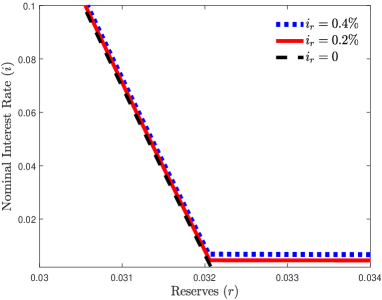
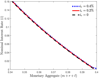
Figure 7: Demand for reserves and the monetary aggregate

Whereas Proposition 1 shows that how the deposit rate can change as the central bank sets the nominal interest rate, the pass-through of nominal interest rate to deposit rate depends on other policy variables and the equilibrium type.

Proposition 4.

Higher reserve requirement weakens the pass-through from the nominal interest rate to the deposit rate in the scarce-reserve equilibrium, i.e.,

$$\frac{\partial^{2}i_{d}}{\partial\chi\partial i}<0\quad\text{ if }\bar{\ell}<\ell^{*}.$$

Higher interest on the reserve raises the pass-through from the nominal interest rate to the deposit rate in the ample-reserves equilibrium, i.e.,

$$\frac{\partial^{2}i_{d}}{\partial i_{r}\partial i}>0\quad\text{ if }\bar{\ell}\geq\ell^{*}.$$

Regardless of the equilibrium type, there exists a downward-sloping demand curve for total liquidity. To illustrate this, I define the monetary aggregate as a sum of cash holdings, reserves, and banknotes in the economy. The right (left) panel of Figure 7 shows that there exist stable downward-sloping demand curves for monetary aggregates (reserves) with different interest on reserves. An increase in $i_{r}$ shifts the money demand to the right, both in the scarce-reserves equilibrium and in the ample-reserves equilibrium. In the scarce-reserves case, higher $i_{r}$ raises $\tilde{r}$ and $\tilde{\ell}$ with a looser lending constraint and shifts the money demand to the right. However, in the ample-reserves equilibrium, higher $i_{r}$ raises reserves $\tilde{r}$ but decreases $\tilde{\ell}$. Last, a rise in $i_{r}$ increases $\bar{i}$, which allows the monetary authority to induce the ample-reserves equilibrium with higher nominal interest rates. As the central bank pays interest on reserves, the economy can shift to the ample-reserves equilibrium, which has a flatter demand curve for reserves. This is consistent with the observation from Nakamura (2018) that the quantity of reserves skyrocketed before interest rates hit zero, but its dramatic increase was simultaneous with the Fed’s introduction of the interest on reserves.

The Role of Access to Unsecured Credit One also can check the effect of changes in the access to unsecured credit, $\sigma_{3}$, or changes in the credit limit, $\bar{\delta}$. An increase in $\sigma_{3}$ implies that more buyers can use unsecured credit in the DM. Some DM2 buyers become DM3 buyers and they hold less deposit than they used to hold. With higher $\bar{\delta}$, although the measure of DM3 buyers stays same, DM3 buyers can use more unsecured credit for the DM trade. As long as there are positive amount of reserve balances, $r>0$, an increase in $\sigma_{3}$ or $\bar{\delta}$ lowers $r$. Appendix A verifies the following:

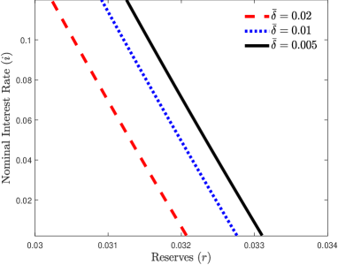
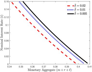
Figure 8: Demand for reserves and the monetary aggregate with different credit limits

Proposition 5.

Let $\hat{\delta}>\bar{\delta}$. In scarce-reserve and ample-reserves equilibria, better credit condition and more credit access decrease the real balance of reserves, i.e.,

$$\frac{\partial r}{\partial\bar{\delta}}<0,\quad\frac{\partial r}{\partial\sigma_{3}}<0.$$

This result is consistent with the finding in Section 2. As more unsecured credit becomes available, real balances of inside money decrease. By summing up the results, we now establish the results on the money multiplier. Define money multiplier $\zeta\equiv(m+r+\ell)/(m+r)$, then we have following results:

Proposition 6.

In ample-reserves equilibrium, for small $m$, we have

$$\frac{\partial\zeta}{\partial i}>0,\quad\frac{\partial\zeta}{\partial i_{r}}<0.$$

Let $\hat{\delta}>\bar{\delta}$. In the ample-reserves and scarce-reserves equilibria, a better credit condition lowers the money multiplier as long as $m>0$ and $\chi<1$, i.e.,

$$\frac{\partial\zeta}{\partial\bar{\delta}}<0\quad\text{ if }m>0\text{ }\&\text{ }\chi<1.$$

Thus, the model can successfully address the mechanism illustrated in Section 2. We can interpret the decline in the money multiplier in the pre-2008 economy as a result of improved availability of consumer credit under the scarce-reserve equilibrium. For the post-2008 period, after the Fed started paying interest on reserves the economy moved to the ample-reserves equilibrium. The model suggests that the changes in the money multiplier and the excess reserve ratio are the results of the Fed’s management of two interest rates, the nominal interest rate and the interest on reserves.

4 Quantitative Analysis

To evaluate the theory quantitatively, I calibrate the model to match several targets using pre-2008 data. Using calibrated parameters, I compare the model predictions with the data of the pre- and post-2008 periods. Given the parameters, the stationary equilibrium is characterized by $(i,i_{r},\chi,\bar{\delta})$. The required reserves ratio is computed by dividing the required reserves by total checkable deposits. Whereas the first three series are easy to obtain, it is hard to get the unsecured credit limit, $\bar{\delta}$, from either macro or micro data. Since the use of unsecured credit corresponds to the credit limit in the model, the unsecured credit limit is computed using the unsecured credit to output ratio, instead of using explicit credit limit data. In the model, the unsecured credit to output ratio is given by $\sigma_{3}\bar{\delta}/(B+\sum_{j}^{3}\sigma_{j}z_{j})$, so we can compute $\bar{\delta}$ using the model with the given policies $(i,i_{r},\chi)$ and other parameters. Following Krueger and Perri (2006), the revolving consumer credit is used as the unsecured credit. For this exercise, I generate simulated data by using 4 series: (i) nominal interest rates; (ii) the interest on reserves; (iii) the required reserve ratio; and (iv) the unsecured credit to GDP ratio.

Table 2: Model parametrization

Parameter	Value	Target/source	Data	Model
External Parameters
DM3 matching prob, $\sigma_{3}$	0.69	SCF 1970-2007
Internal Parameters
Bargaining power, $\theta$	0.454	avg. retail markup	$1.384$	$1.384$
Enforcement cost level, $E$	0.001	avg. $UC/DM$	$0.387$	$0.370$
Deposit operating cost level, $A$	0.0017	avg. $R/Y$	$0.014$	$0.017$
Entry cost, $k$	0.0011	avg. $\Pi/Y$	$0.0016$	$0.0011$
DM1 matching prob, $\sigma_{1}$	0.187	avg. $C/D$	$0.529$	$0.523$
DM utility level, $B$	0.825	avg. $C/Y$	$0.044$	$0.044$
DM utility curvature, $b$	0.398	semi-elasticity of $C/Y$ to $i$	$-3.713$	$-3.712$

• Note: $C$, $R$, $DM$, $D$, $UC$, and $Y$ denote currency in circulation, reserves, DM transactions, deposit, unsecured credit, and nominal output, respectively. $\Pi$ denotes the net income of banks.

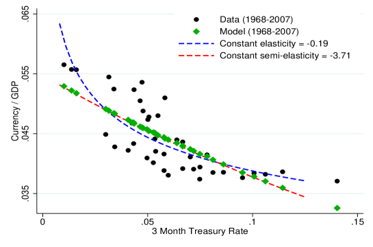
Figure 9: Money demand for currency

4.1 Calibration

The utility functions for the DM and the CM are $u(q)=Bq^{1-b}/(1-b)$ and $U(X)=\log(X)$ implying $X^{*}=1$ (a normalization). The cost function for the DM is $c(q)=q$. The enforcement cost for lending is assumed to be quadratic, $\eta(\tilde{\ell})=E\tilde{\ell}^{2}$, and the management cost for deposit facility takes the form, $\gamma(\tilde{d})=A\tilde{d}^{a}$. The fraction of buyers who can use unsecured credit is set to $\sigma_{3}=0.69$. The remaining 7 parameters $(\theta,A,B,b,k,E,\sigma_{1})$ are set to match the following eight targets: (i) the average retail market markup; (ii) the average credit share of the DM transactions, $\sigma_{3}\delta/DM$; (iii) the average currency to deposit ratio, $C/D$; (iv) the average reserves to output ratio, $R/Y$; (v) the average currency to output ratio, $C/Y$; (vi) the semi-elasticity of $C/Y$ to $i$, where $i$ denotes the nominal interest rate; and (vii) the average net income of banks to output ratio; (viii) the average net income of banks to deposit ratio. The targets are computed on the basis of 1968-2007 data, except for the markup, which uses the average from 1993 to 2007, and the net income of banks, which uses the average from 1984 to 2007.

The bargaining power $\theta$ is set to match the DM markup to the retail markup. Set $(B,b)$ to match the currency to output ratio and the semi-elasticity of $C/Y$ with respect to $i$. The costs of operating deposit services and issuing loans from the bank, captured by $A$ and $E$, are set to match the reserves to output ratio, the unsecured credit to DM transaction ratio and the banking industry profit to deposit ratio. The entry cost $k$ is set to match banking industry profit to output ratio. Lastly, I set $\sigma_{1}$ to match the currency-deposit ratio. The calibrated parameters and the targets are summarized in Table 2, and the calibrated money demand of currency is shown in Figure 9.

4.2 Results and the Model Fit

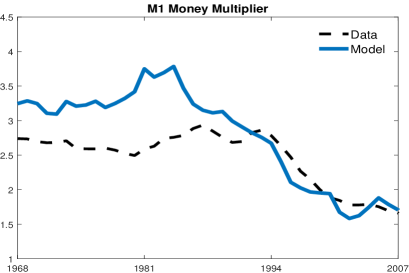
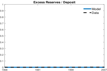
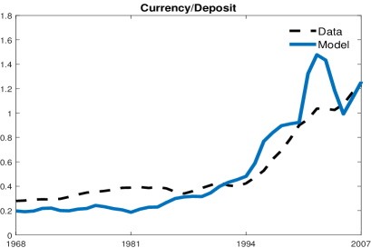
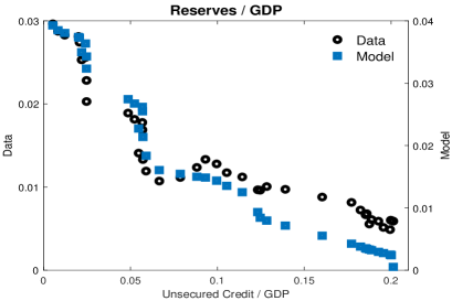
Figure 10: In-sample fit: 1968-2007

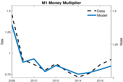
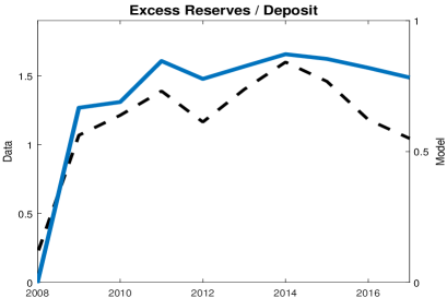
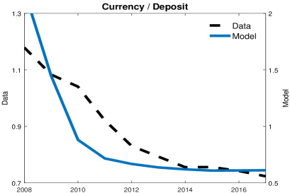
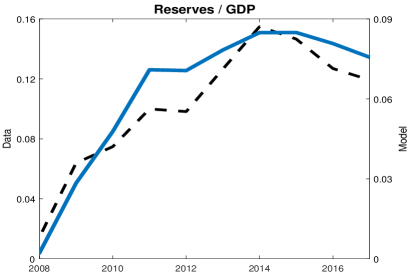
Figure 11: Out-of-sample fit: 2008-2017

Figure 10 compares the model and data for the sample period, 1968 to 2007. The top-left panel of Figure 10 shows the M1 money multiplier from 1968 to 2007. The model generated decreases in the M1 multiplier during 1987-2007, while the peak was in 1987 in the data and 1984 in the model. During this period, the excess reserves to deposit ratio had been almost zero both in the data and in the model, suggesting the US economy had been in the scarce-reserves equilibrium. In the model, the declining trend of the M1 multiplier in the pre-2008 period is driven by the increase in unsecured credit, which crowds out the inside money (private banknotes and reserves) but not currency. This induces increases in the currency to deposit ratio, as shown in the bottom-left panel of Figure 10. The bottom-right panel of Figure 10 compares how unsecured credit crowds out reserves in the model and the data.

The next step is to evaluate model projections by comparing them with the data after 2007. Overall, the model can match the patterns in the data. Timeplots of Figure 11 compares the model projections for the M1 money multiplier, the excess reserves to deposit ratio, the currency to deposit ratio, and the reserves to output ratio with data from 2008 to 2017. The model-implied series shows similar patterns to the actual data series. The model can generate the change in the equilibrium type, from scarce-reserves to ample-reserves, and a similar pattern of excess reserves to deposit ratio. This change in the equilibrium type is represented by a huge drop in the money multiplier in the top-left panel and a huge increase in the excess reserves to deposit ratio in the top-right panel.

Regression estimates shown in Table 3 illustrate the main mechanism of the model. Columns (1) and (2) show the regression coefficient estimates using the following equation for 1968-2007.

$$\text{Reserves}_{t}/\text{GDP}_{t}=\beta_{0}+\beta_{1}\text{UnsecuredCredit}_{t}/\text{GDP}_{t}+\beta_{2}\texttt{Tbill3}_{t}+\epsilon_{t}$$

Since all three series have a unit root and are cointegrated, both in the data and in the model-generated series, the coefficients are estimated using the canonical cointegrating regression. The estimated negative coefficient on the 3-month T-bill rate suggests a downward sloping demand for reserves with respect to the interest rate; but other coefficients on unsecured credit suggest that this demand for reserves can shift as the credit condition changes, as shown in Figure 8. This is consistent with Proposition 5, and the model-implied regression produces similar results.

Table 3: Model-implied regression coefficients, model vs. data

Dependent Variable:	Reserves/GDP		M1 Money Multiplier		Excess Reserve/Deposit
	(1968-2007)		(2009-2017)		(2009-2017)
	Data	Model	Data	Model	Data	Model
	(1)	(2)	(3)	(4)	(5)	(6)
Unsecured Credit/GDP	$-0.125^{***}$	$-0.200$
	$(0.010)$
3 Month T-bill Rate	$-0.001^{***}$	$-0.001$	$0.686^{***}$	$0.864$	$-1.561^{***}$	$-1.697$
	$(0.000)$		$(0.184)$		$(0.498)$
Interest on Reserves			$-0.648^{***}$	$-0.848$	$1.461^{**}$	$1.688$
			$(0.210)$		$(0.567)$
$adjR^{2}$	$0.830$	$0.814$	$0.656$	$0.918$	$0.577$	$0.997$

• Notes: Columns (1)-(2) report the canonical cointegrating regression (CCR) estimates. First stage long-run variance estimation for CCR is based on Bartlett kernel and lag 1. Columns (3)-(6) report OLS estimates. For (3) and (5) Newey-West standard errors with lag 1 are reported in parentheses. ***, **, and * denote significance at the 1, 5, and 10 percent levels, respectively. Intercepts are included but not reported.

Columns (3) and (4) regress the M1 multiplier on the 3 month T-bill rate and the interest on reserves, and Columns (5) and (6) regress the excess reserves ratio on the same variables. Because the number of observations in the data is too small, Columns (3) and (5) use data from the 1st quarter of 2009 to the 4th quarter of 2017. Regressions using the data and the model-implied series provide similar results. Based on the regression results in (3)-(6), for a given interest on reserves, raising the 3-month T-bill rates increases the M1 multiplier while it decreases excess reserves. At the same time, for a given 3-month treasury rate, lowering the interest on reserves decreases the M1 multiplier while it increases excess reserves. In the model, when the bank faces higher interests on reserves, it holds more reserves and does not lend as much as before. This is because interest on reserves yields profits to the bank with low cost, but lending is associated with the enforcement cost. This increases the excess reserve ratio and lowers the money multiplier. The model also provides the composition of the monetary base over time. Figure 12 compares the composition of the monetary base from the data and the model. The model successfully generates the changes for each component of the monetary base - currency, required reserves, and excess reserves - both before and after 2008.

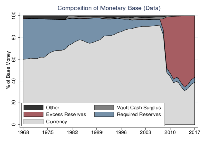
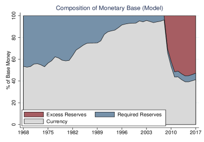
Figure 12: Composition of monetary base: data vs. model

A Digression on Model Fit For the post-2007 period, although the model projections can match the patterns in the data well, they do not fit very well in levels. This discrepancy is from the fact that the theoretical lower bound for the money multiplier is 1 in the model. In reality, however, the U.S. economy has experienced M1 multipliers lower than 1. There are two potential explanations for this.

One possible reason is that monetary policy can be conducted in different ways than the lump-sum transfer in the model. In the model, all the base money is distributed to agents through the lump-sum transfer, and they keep some in their bank accounts. Reserves are in the bank deposits in this setup, and this implies the money multiplier can not be lower than 1. In contrast to most of the monetary models that assume money is injected as a lump-sum transfer across the agents (buyers and sellers, in this model), much money injection is made to the banking system directly in the real economy. For example, in the quantitative easing program, the Fed purchased large amounts of financial assets from financial intermediaries and gave them the same amount in reserves. These reserves are directly injected into the banking system and this is different from lump-sum transfers. In this case, reserves can only be held by banks, not by the public, and banks do not lend out reserves. One may need to consider a more explicit mechanism for monetary policy implementation.

Another possible reason is that reserves could be kept in saving accounts or time deposits, which is in M2 but not in M1. Even though one assumes that the monetary base is distributed through a lump-sum transfer, it does not have to be kept in a checkable account. In this case, there is no discrepancy between the data and the theoretical lower bound for the money multiplier because the M2 money multiplier has never been lower than 1. From a balance sheet point of view, reserves are recorded as a cash asset on the commercial bank’s balance sheet because reserves are held as an account for the commercial banks at the Federal Reserve Bank, but deposits are liabilities. In this case, reserves cannot exceed total liabilities (total deposits), but they can exceed checkable deposits.

4.3 Welfare

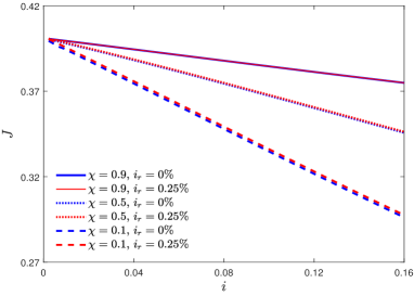
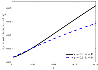
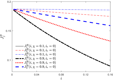
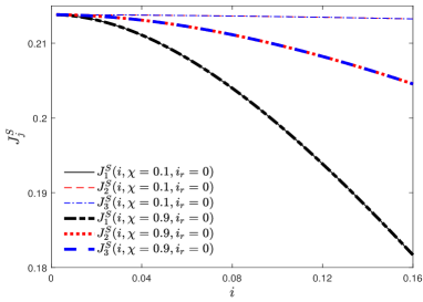
Figure 13: Welfare

So far, I have shown that different tools of monetary policy have distinct roles in monetary transmission. This section focuses on the impacts of these different tools of monetary policy in terms of welfare. I measure the welfare of the seller in type $j$ meeting using her DM trade surplus.

$$J^{S}_{j}(i,\chi,i_{r})=(1-\theta)[u(q_{j})-c(q_{j})],$$

and the welfare of the buyer who trades in the $j$ type DM meeting is a DM trade surplus with the cost for acquiring the cash and reserves.

$$J^{B}_{j}(i,\chi,i_{r})=-im_{j}(i,\chi,i_{r})-(i-i_{d})r_{j}(i,\chi,i_{r})+(1-\theta)[u(q_{j})-c(q_{j})]$$

I define the total welfare as a weighted sum of each agent’s welfare.

$$J(i,\chi,i_{r})=\sum_{j=1}^{3}\sigma_{j}[J^{B}_{j}(i,\chi,i_{r})+J^{S}_{j}(i,\chi,i_{r})]$$

The top-left panel of Figure 13 illustrates the effects of monetary policy, $i$, on total welfare $J$ ranging from 0% to 16% and how its impact can change depending on different reserve requirements and different interest rates on reserves. Each curve denotes the welfare under the different reserve requirements and interest rates on reserves. The welfare is monotonically decreasing in $i$, and each curve can be shifted up by paying interest on reserves or lowering the reserve requirement. These results are well expected. The higher opportunity cost of holding money lowers welfare. Paying interest on reserves, however, is welfare improving because it compensates the opportunity cost of holding money. Lowering reserve requirement also improves welfare since it provides more liquidity to the economy. The difference becomes smaller as the economy faces lower $i$, and the Friedman rule gives the optimal level of welfare.

In addition to total welfare, one can examine the distributional effect of monetary policy. The top-right panel of Figure 13 plots the standard deviation of each agent’s welfare, $J^{k}_{j}$ under different policies. Clearly, the effects of the monetary policy are different across the agents. The bottom-left (bottom-right) panels of Figure 13 plots the buyer’s (seller’s) welfare in different DM meetings depending on different policies. Among buyers, DM1 buyer’s welfare is lower than others. Whereas DM2 and DM3 buyers consume the same amount in the DM, given that the access to unsecured credit allows the DM3 buyer carry less money than the DM2 buyer, the DM3 buyer’s welfare is higher than the DM2 buyer’s. For the sellers, because the consumption in DM2 and DM3 are equal, they enjoy the same welfare. As in the buyers’ case, DM1 seller’s welfare is the lowest among all the sellers. Lowering reserve requirement increases the welfare of buyers and sellers in DM2 and DM3. However, DM1 agents’ welfare is independent of reserves requirement, access to credit, and the interest on reserves but only depends on the nominal interest rate.

4.4 Counterfactual Analysis

In this section, I use calibrated parameters to assess how the money multiplier and currency deposit ratio would be changed by setting different reserve requirements. I also demonstrate that it is important to distinguish the effect of the reserve requirement from the effect of credit.

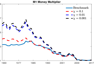
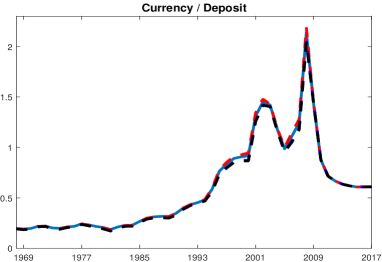
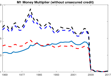
Figure 14: Counterfactual analysis

The top panel of Figure 14 shows the counterfactual under different reserve requirements while keeping $(i,i_{r},\bar{\delta})$ the same as in the benchmark case. With a lower reserve requirement, the money multiplier increases. However, we see a trend of decreasing multipliers regardless of reserve requirement. As illustrated in Table 3, this gradual decrease in the money multiplier since the late 1980s is driven by an increase in unsecured credit in the model. The currency deposit ratio increases with a higher reserve requirement and all the cases show the similar trend.

The bottom panel of Figure 14 shows the counterfactual under a different reserve requirement with $\bar{\delta}=0$, and $(i,i_{r})$ set to the data. In the bottom-right panel, we see almost no changes in the currency deposit ratio. Since the money demand for currency and inside money is stable, if unsecured credit did not crowd out inside money, there would not be a substantial increase in the currency deposit ratio, as the U.S. economy witnessed. In the case of the money multiplier, whereas it shows a stationary pattern before 2009, it drops drastically once the Federal Reserve started paying interest on reserves and lowered the nominal interest rate. This suggests that the gradual decline of the money multiplier from the late 1980s to 2007 can be attributed to an increase in unsecured credit, whereas the dramatic decline in the money multiplier since 2008 can be explained by the monetary policies of the Federal Reserve.

4.5 Robustness

This section briefly summaries a few results from Appendix C. Appendix C.1 examines the sensitivity of the results using different measures of the monetary policy target: the federal funds rate, and the commercial paper rate. Using different measures does not change the main results. In Appendix C.2, to check whether the curvature parameter 1.2 for the deposit operating cost is sensitive, I change the benchmark parameter from 1.2 to 1.15 or 1.25. Changing these parameters does not have a significant impact on the results.

5 Concluding Remarks

This paper develops a monetary-search model with fractional banking and unsecured credit and studies the money creation process. In the fractional reserve system, the money is created when banks make loans. The bank’s lending, however, can be constrained by the reserve requirement and the reserves.

Banks hold excess reserves when the central bank pays sufficiently high interest on reserves with the nominal interest rate at some moderate level. In this case, the money multiplier and the quantity of the reserve depend on the nominal interest rate and the interest on reserves rather than the reserve requirement. In contrast to the previous works, these two interest rates play distinct roles. Whether the banks hold excess reserves or not, there exists a downward-sloping demand curve for reserves, and the Friedman rule is optimal. Paying interest on reserves with low nominal interest rates can move the economy from the scarce reserves regime to the ample reserves regime, which is consistent with what we have seen in the US economy. The quantitative analysis can generate simulated data that resemble the actual data. This paper provides evidence from the model and the data that suggests that the dramatic changes in the money multiplier after 2008 are mainly driven by the introduction of the interest on reserves with the low nominal interest rate.

This work can be extended in various ways. Although I focus on the centralized market for the reserves with homogeneous banks, in reality, the market for reserves is a decentralized interbank market and banks have different portfolios. Therefore, one can further investigate how much the market structure and heterogeneity matter for the transmission of monetary policy (e.g., Afonso and Lagos, 2015; Armenter and Lester, 2017; Afonso, Armenter and Lester, 2019). Second, it would be worthwhile to study how inside creation via loan extension is related to investment and firms’ dynamics (e.g., Ennis, 2018; Bianchi and Bigio, 2014; Altermatt, 2019). This will allow us to understand the investment channels of monetary policy more explicitly. Moreover, I assume that bank assets are composed of loans and reserves. But commercial banks’ assets are mainly composed of securities, loans, and reserves. Extending the model to incorporate banks’ portfolio choices and analyzing the role of investment, financial regulation, and monetary policy can open up other research avenues. (e.g., Rocheteau, Wright and Zhang, 2018a).

Appendix

Appendix A Proofs

Proof of Proposition 1.

First, consider the ample-reserves equilibrium. Each bank’s the real balance of reserves, $\tilde{r}$, and lending, $\tilde{\ell}$, are determined by following two equations

$$0 =\underbrace{\frac{1+i}{1+i_{r}-\gamma^{\prime}(\tilde{r})}-1-\eta^{\prime}(\tilde{\ell})}_{P}$$ (30)

$$0 =\underbrace{\gamma^{\prime}(\tilde{r})\tilde{r}-\gamma(\tilde{r})+\eta^{\prime}(\tilde{\ell})\tilde{\ell}-\eta(\tilde{\ell})-k}_{E}$$ (31)

where $\frac{1+i}{1+i_{r}-\gamma^{\prime}(\tilde{r})}\geq 1$. By the implicit function theorem, we have

$$P_{r}d\tilde{r}+P_{\ell}d\tilde{\ell}+P_{i}di+P_{i_{r}}di_{r} =0$$ (32)

$$E_{r}d\tilde{r}+E_{\ell}d\tilde{\ell}+E_{i}di+E_{i_{r}}di_{r} =0$$ (33)

where

$$\begin{array}[]{lcl}P_{r}=(1+i)\gamma^{\prime\prime}(\tilde{r})/\{1+i_{r}-\gamma^{\prime}(\tilde{r})\}^{2}&&E_{r}=\gamma^{\prime\prime}(\tilde{r})\tilde{r}\\ P_{\ell}=-\eta^{\prime\prime}(\tilde{\ell})&&E_{\ell}=\eta^{\prime\prime}(\tilde{\ell})\tilde{\ell}\\ P_{i}=1/\{1+i_{r}-\gamma^{\prime}(\tilde{r})\}&&E_{i}=0\\ P_{i_{r}}=-(1+i)/\{1+i_{r}-\gamma^{\prime}(\tilde{r})\}^{2}&&E_{i_{r}}=0.\end{array}$$

Applying Cramer’s Rule to (32)-(33) yields the following comparative statics results:

$$\frac{\partial\tilde{\ell}}{\partial i}=\frac{P_{i}E_{r}}{P_{r}E_{\ell}-P_{\ell}E_{r}}>0,\quad\frac{\partial\tilde{r}}{\partial i}=\frac{-P_{i}E_{\ell}}{P_{r}E_{\ell}-P_{\ell}E_{r}}<0$$

$$\frac{\partial\tilde{\ell}}{\partial i_{r}}=\frac{P_{i_{r}}E_{r}}{P_{r}E_{\ell}-P_{\ell}E_{r}}<0,\quad\frac{\partial\tilde{r}}{\partial i_{r}}=\frac{-P_{i_{r}}E_{\ell}}{P_{r}E_{\ell}-P_{\ell}E_{r}}>0.$$

From the above results, we can get immediate results: $\partial i_{d}/\partial i>0$ and

$$\frac{\partial i_{d}}{\partial i_{r}}=1-\frac{1+i}{1+i+[1+i_{r}-\gamma^{\prime}(\tilde{r})]}>0$$ (34)

since $i_{d}=i_{r}-\gamma^{\prime}(\tilde{r})>0$.

Given $\partial\tilde{\ell}/\partial i_{r}<0$, $\partial\tilde{\ell}/\partial i>0$ and $i_{\ell}=\eta(\tilde{\ell})$, we have $\partial i_{\ell}/\partial i_{r}<0$ and $\partial i_{\ell}/\partial i>0$, which implies that, in DM2, $L^{-1}(i_{\ell})$ is increasing in $i_{r}$ and decreasing in $i$.

Now consider the no-banking equilibrium. The no-banking equilibrium satisfies

$$i=L(m_{j})\text{ for }j=1,2,\quad m_{3}=\max\{0,L^{-1}(i)-\bar{\delta}\}$$

with $r=0$, $i_{d}=0$ and $n=0$. In the no-banking case, it is straight forward to show

$$\frac{\partial r}{\partial i}=0,\quad\frac{\partial i_{d}}{\partial i}=0,\quad\frac{\partial r}{\partial i_{r}}=0,\quad\frac{\partial i_{d}}{\partial i_{r}}=0.$$

In the scarce-reserve equilibrium, $\tilde{r}$ is determined by

$$(i_{r}-i_{d})\tilde{r}+i_{\ell}\frac{1-\chi}{\chi}\tilde{r}-\gamma\left(\tilde{r}\right)-\eta\left(\frac{1-\chi}{\chi}\tilde{r}\right)=k$$

$$i_{r}-i_{d}-\gamma^{\prime}(\tilde{r})+\Bigg{[}i_{\ell}-\eta^{\prime}\left(\frac{1-\chi}{\chi}\tilde{r}\right)\Bigg{]}\frac{1-\chi}{\chi}=0,$$

where $i_{\ell}=\frac{1+i}{1+i_{d}}-1$. This implies that $\tilde{r}$ solves

$$\gamma^{\prime}(\tilde{r})\tilde{r}-\gamma(\tilde{r})+\eta^{\prime}\left(\frac{1-\chi}{\chi}\tilde{r}\right)\frac{1-\chi}{\chi}\tilde{r}-\eta\left(\frac{1-\chi}{\chi}\tilde{r}\right)=k$$ (35)

which is independent of $i$ and $i_{r}$. The right-hand side of (35) is a positive constant, $k>0$. Because the left-hand side of (35) is equal to 0 when $\tilde{r}=0$ and strictly increasing in $\tilde{r}$, equation (35) uniquely pins down $\tilde{r}$. Let’s define this $\tilde{r}$ as $\hat{r}$. The equilibrium deposit rate can be expressed as

$$i_{d}=i_{r}-\gamma^{\prime}(\hat{r})+\left[\frac{1+i}{1+i_{d}}-1-\eta^{\prime}\left(\frac{1-\chi}{\chi}\hat{r}\right)\right]\frac{1-\chi}{\chi}>0.$$ (36)

Because $\hat{r}$ is independent of $i$ and $i_{r}$, the implicit function theorem yields $\frac{\partial i_{d}}{\partial i_{r}}=1+\frac{(1-\chi)(1+i)}{\chi(1+i_{d})^{2}}>0$ and

$$\frac{\partial i_{d}}{\partial i}=\left[\frac{\chi(1+i_{d})}{1-\chi}+\frac{1+i}{1+i_{d}}\right]^{-1}>0.$$ (37)

Using above results, one can show that

$$\frac{\partial i_{\ell}}{\partial i}=\frac{(1+i_{d})\chi}{(1+i)(1-\chi)+\chi(1+i_{d})^{2}}>0,\quad\frac{\partial i_{\ell}}{\partial i_{r}}=-\frac{1+i}{(1+i_{d})^{2}}\frac{\partial i_{d}}{\partial i_{r}}<0.$$

∎

Proof of Proposition 2.

First, consider the ample-reserves equilibrium. Each bank’s real balance of reserves, $\tilde{r}$, and lending, $\tilde{\ell}$, are determined by equations (30)-(31). By applying implicit function theorem to (32),

$$\frac{\partial\tilde{r}}{\partial\tilde{\ell}}=-\frac{\partial P_{\ell}}{\partial P_{r}}=\frac{\eta^{\prime\prime}(\tilde{\ell})[1+i_{r}-\gamma^{\prime}(\tilde{r})]^{2}}{(1+i)\gamma^{\prime\prime}(\tilde{r})}>0.$$

By applying implicit function theorem to (33),

$$\frac{\partial\tilde{r}}{\partial\tilde{\ell}}=-\frac{\partial E_{\ell}}{\partial E_{r}}=-\frac{\gamma^{\prime\prime}(\tilde{r})\tilde{r}}{\eta^{\prime\prime}(\tilde{\ell})\tilde{\ell}}<0.$$

By (30), $\tilde{r}=\max\{0,\gamma^{\prime-1}(i_{r}-i)\}$ when $\tilde{\ell}=0$. Define this $\tilde{r}$ as $\tilde{r}_{1}$. By equation (31), $\tilde{r}>0$ when $\tilde{\ell}=0$, where $\tilde{r}_{2}$ solves $\gamma^{\prime}(\tilde{r})\tilde{r}-\gamma(\tilde{r}_{2})=k$. Define this $\tilde{r}$ as $\tilde{r}_{2}$. Therefore equations (30)-(31) have a single crossing point in $\mathbb{R}^{2}_{+}$ space as long as $\tilde{r}_{1}<\tilde{r}_{2}$. This condition ($\tilde{r}_{1}<\tilde{r}_{2}$) is satisfied under the ample-reserves equilibrium, which will be shown at the end of this proof.

Given this and $i_{\ell}=(1+i)/(1+i_{d})-1$, $n$ solves

$$(\sigma_{2}+\sigma_{3})L^{-1}(i_{\ell})-\sigma_{3}\bar{\delta}=n(\tilde{r}+\tilde{\ell})$$ (38)

when $\hat{\delta}>\bar{\delta}$, whereas $n$ solves

$$\sigma_{2}L^{-1}(i_{\ell})=n(\tilde{r}+\tilde{\ell})$$

when $\hat{\delta}\leq\bar{\delta}$. Because $n$ is uniquely determined by above equations, solving for the ample-reserves equilibrium provides unique solution.

Now consider the scarce-reserve equilibrium. Recall that (35) uniquely pins down $\tilde{r}$. Given $\tilde{r}$, $i_{d}$ is uniquely determined by (36). Given $i_{\ell}=\frac{1+i}{1+i_{d}}-1$, $n$ solves

$$(\sigma_{2}+\sigma_{3})L^{-1}(i_{\ell})-\sigma_{3}\bar{\delta}=n\tilde{r}\left(\frac{1+\chi i_{d}}{\chi}\right)$$ (39)

when $\hat{\delta}>\bar{\delta}$, whereas $n$ solves

$$\sigma_{2}L^{-1}(i_{\ell})=n\tilde{r}\left(\frac{1+\chi i_{d}}{\chi}\right)$$

when $\hat{\delta}\leq\bar{\delta}$. Because $n$ is uniquely determined by above equations, it is straightforward to show that there is an unique solution.

In case of the no banking equilibrium, the equilibrium satisfies $i=L(m_{j})$ for $j=1,2$ and $m_{3}=\max\{0,L^{-1}(i)-\bar{\delta}\}$, which yield an unique solution.

The next step is characterizing the equilibrium type for given policies. When bank’s unconstrained optimal lending $\ell^{*}=\eta^{\prime-1}(i_{\ell})$ is bigger than $\bar{\ell}$, the equilibrium is a scarce reserve equilibrium, whereas when $\bar{\ell}>\ell^{*}=\eta^{\prime-1}(i_{\ell})$, the equilibrium is an ample-reserves equilibrium. There exists a threshold $\bar{i}$ that satisfies $\bar{\ell}=\ell^{*}$ and

$$\bar{i}=[1+i_{r}-\gamma^{\prime}(\hat{r})]\left[1+\eta^{\prime}\left(\frac{1-\chi}{\chi}\hat{r}\right)\right]-1.$$

Because $\partial\tilde{r}/\partial i<0$ and $\bar{\ell}=\tilde{r}(1-\chi)/\chi$, it is straightforward to show $\partial\bar{\ell}/\partial i<0$ and $\partial\ell^{*}/\partial i>0$. Therefore, $\bar{i}$ is a threshold above which the equilibrium is a scarce reserve equilibrium and below which the equilibrium is an ample-reserves equilibrium.

The no-banking equilibrium arises when the equilibrium deposit rate $i_{d}$ is zero and lowering $i$ decreases the deposit rate. The threshold between the no-banking case and the scarce-reserve case $\hat{i}$ satisfies $i_{d}=i_{r}-\gamma^{\prime}(\tilde{r})+\left[\frac{1+\hat{i}}{1+i_{d}}-1-\eta^{\prime}\left(\frac{1-\chi}{\chi}\tilde{r}\right)\right]\frac{1-\chi}{\chi}=0$, implying

$$\hat{i}=\frac{\chi}{1-\chi}[\gamma^{\prime}(\hat{r})-i_{r}]+\eta^{\prime}\left(\frac{1-\chi}{\chi}\hat{r}\right).$$

When $i<i_{d}$, there is no equilibrium in the market for reserves since demand for reserves is infinite. In this this case, there is no equilibrium with banks. The threshold that satisfies $i=i_{d}$ is $\underline{i}=i_{r}-\gamma^{\prime}(\underline{r})$ where $\underline{r}$ solves $\gamma^{\prime}(\underline{r})\underline{r}-\gamma(\underline{r})=k$. Since the ample-reserve equilibrium always satisfies $i>\underline{i}$, the condition for the existence of a unique ample-reserve equilibrium, $\tilde{r}_{1}<\tilde{r}_{2}$, is satisfied.

Therefore, we can conclude that given $(i_{r},\chi)$: (i) $\exists!$ ample-reserves equilibrium if and only if $i_{r}>\gamma^{\prime}(\hat{r})$ and $i\in(\underline{i},\bar{i})$; (ii) $\exists!$ scarce-reserves equilibrium if and only if either $i>\hat{i}$ and $i_{r}<\gamma^{\prime}(\hat{r})$ or $i>\bar{i}$ and $i_{r}>\gamma^{\prime}(\hat{r})$; (iii) $\exists!$ no banking equilibrium if and only if either $i\in[0,\hat{i})$ and $i_{r}<\gamma^{\prime}(\hat{r})$, or $i\in[0,\underline{i})$ and $i_{r}>\gamma^{\prime}(\underline{r})$. ∎

Proof of Corollary 1.

Because $\underline{r}$ solves $\gamma^{\prime}(\underline{r})\underline{r}-\gamma(\underline{r})=k$, $\underline{r}$ is independent of $i_{r}$. Therefore, given $\underline{i}=i_{r}-\gamma^{\prime}(\underline{r})$, $\partial\underline{i}/\partial i_{r}=1>0$. Similarly, because $\hat{r}$ solves $\gamma^{\prime}(\hat{r})\hat{r}-\gamma(\hat{r})+\eta^{\prime}\left(\frac{1-\chi}{\chi}\hat{r}\right)\frac{1-\chi}{\chi}\hat{r}-\eta\left(\frac{1-\chi}{\chi}\hat{r}\right)=k$, $\hat{r}$ is independent of $i_{r}$. Therefore, given

$$\hat{i}=\frac{\chi}{1-\chi}[\gamma^{\prime}(\hat{r})-i_{r}]+\eta^{\prime}\left(\frac{1-\chi}{\chi}\hat{r}\right),\quad\bar{i}=[1+i_{r}-\gamma^{\prime}(\hat{r})]\left[1+\eta^{\prime}\left(\frac{1-\chi}{\chi}\hat{r}\right)\right]-1,$$

we have $\partial\hat{i}/\partial i_{r}=\frac{-\chi}{1-\chi}<0$ and $\partial\bar{i}/\partial i_{r}=\left[1+\eta^{\prime}\left(\frac{1-\chi}{\chi}\hat{r}\right)\right]>0$.

∎

Proof of Proposition 4.

First, consider the scarce-reserve equilibrium. Recall equations (35) and (36)

$$0 =\underbrace{\gamma^{\prime}(\tilde{r})\tilde{r}-\gamma(\tilde{r})+\eta^{\prime}\left(\frac{1-\chi}{\chi}\tilde{r}\right)\frac{1-\chi}{\chi}\tilde{r}-\eta\left(\frac{1-\chi}{\chi}\tilde{r}\right)-k}_{\Omega}$$

$$0 =\underbrace{-i_{d}+i_{r}-\gamma^{\prime}(\tilde{r})+\left[\frac{1+i}{1+i_{d}}-1-\eta^{\prime}\left(\frac{1-\chi}{\chi}\tilde{r}\right)\right]\frac{1-\chi}{\chi}}_{\Lambda}.$$

Applying the implicit function theorem yields

$$\left[\begin{array}[]{cc}\Omega_{i_{d}}&\Omega_{r}\\ \Lambda_{i_{d}}&\Lambda_{r}\end{array}\right]\left[\begin{array}[]{c}di_{d}/d\chi\\ d\tilde{r}/d\chi\end{array}\right]=\left[\begin{array}[]{c}-\Omega_{\chi}\\ -\Lambda_{\chi}\end{array}\right]$$

where

$$\begin{array}[]{lcl}\Omega_{i_{d}}=0,&&\Lambda_{i_{d}}=-1-\frac{(1+i)(1-\chi)}{\chi(1+i_{d})^{2}}\\ \Omega_{r}=\gamma^{\prime\prime}(\cdot)\tilde{r}+\eta^{\prime\prime}(\cdot)\left(\frac{1-\chi}{\chi}\right)^{2}\tilde{r},&&\Lambda_{r}=\gamma^{\prime\prime}(\cdot)-\left(\frac{1-\chi}{\chi}\right)^{2}\eta^{\prime\prime}(\cdot)\\ \Omega_{\chi}=-\frac{1-\chi}{\chi^{3}}\tilde{r}^{2}\eta^{\prime\prime}(\cdot),&&\Lambda_{\chi}=\frac{1-\chi}{\chi^{3}}\tilde{r}\eta^{\prime\prime}(\cdot)-\frac{1}{\chi^{2}}\left[\frac{1+i}{1+i_{d}}-1-\eta^{\prime}(\cdot)\right].\end{array}$$

By Cramer’s rule,

$$\frac{\partial i_{d}}{\partial\chi}=\frac{\left|\begin{array}[]{cc}-\Omega_{\chi}&\Omega_{r}\\ -\Lambda_{\chi}&\Lambda_{r}\end{array}\right|}{\left|\begin{array}[]{cc}\Omega_{i_{d}}&\Omega_{r}\\ \Lambda_{i_{d}}&\Lambda_{r}\end{array}\right|}=-\frac{\frac{1}{\chi^{2}}\left[\frac{1+i}{1+i_{d}}-1-\eta^{\prime}\left(\frac{1-\chi}{\chi}\hat{r}\right)\right]}{1+\frac{(1+i)(1-\chi)}{\chi(1+i_{d})^{2}}}<0.$$

Recall (37) $\frac{\partial i_{d}}{\partial i}=\left[\frac{\chi(1+i_{d})}{1-\chi}+\frac{1+i}{1+i_{d}}\right]^{-1}$, by taking a derivative with respect to $\chi$

$$\frac{\partial i_{d}}{\partial\chi\partial i}=\frac{-(1+i_{d})}{(1-\chi)^{2}[1+i+\frac{\chi}{1-\chi}(1+i_{d})]^{2}}+\frac{1+i}{[1+i+\frac{\chi}{1-\chi}(1+i_{d})^{2}]^{2}}\frac{\partial i_{d}}{\partial\chi}<0$$

because $\frac{\partial i_{d}}{\partial\chi}<0$.

Now consider the ample-reserve equilibrium. Recall equation (34) from the ample reserve case,

$$\frac{\partial i_{d}}{\partial i_{r}}=1-\frac{1+i}{1+i+[1+i_{r}-\gamma^{\prime}(\tilde{r})]}.$$

Taking derivative with respect to $i$ gives the following

$$\frac{\partial^{2}i_{d}}{\partial i\partial i_{r}} =\frac{-[1+i_{r}-\gamma^{\prime}(\cdot)]-(1+i)\gamma^{\prime\prime}(\cdot)\frac{\partial\tilde{r}}{\partial i}}{\{2+i+i_{r}-\gamma^{\prime}(\cdot)\}^{2}}$$

$$=\frac{[1+i_{r}-\gamma^{\prime}(\cdot)]^{3}}{\{2+i+i_{r}-\gamma^{\prime}(\cdot)\}^{2}\{\ell+[1+i_{r}-\gamma^{\prime}(\cdot)]^{2}\}}>0$$

using the results from the proof of Proposition 1. ∎

Proof of Proposition 5.

Assume $\hat{\delta}>\bar{\delta}$. For the scarce reserve equilibrium, recall (29)

$$r=\frac{(\sigma_{2}+\sigma_{3})\chi}{1+i_{d}\chi}L^{-1}(i_{\ell})-\frac{\sigma_{3}\bar{\delta}\chi}{1+i_{d}\chi}.$$

Given $\hat{\delta}>\bar{\delta}$, it is straightforward to show that

$$\frac{\partial r}{\partial\bar{\delta}}=\frac{-\sigma_{3}\chi}{1+i_{d}\chi}<0,\quad\frac{\partial r}{\partial\sigma_{3}}=\frac{-\bar{\delta}\chi}{1+i_{d}\chi}<0.$$

For the ample reserve equilibrium, recall (38)

$$(\sigma_{2}+\sigma_{3})L^{-1}(i_{\ell})-\sigma_{3}\bar{\delta}=n(\tilde{r}+\tilde{\ell}).$$

Because $\tilde{r}$, $\tilde{\ell}$, $i_{d}$, and $i_{\ell}$ are independent of $\bar{\delta}$, we have

$$\frac{\partial n}{\partial\bar{\delta}}=\frac{-\sigma_{3}}{\tilde{r}+\tilde{\ell}}<0,\quad\frac{\partial n}{\partial\sigma_{3}}=\frac{-\bar{\delta}}{\tilde{r}+\tilde{\ell}}<0$$

implying $\frac{\partial r}{\partial\bar{\delta}}<0$ and $\frac{\partial r}{\partial\sigma_{3}}<0$ where $r=n\tilde{r}$. ∎

Proof of Proposition 6.

Define money multiplier $\zeta\equiv(m+r+\ell)/(m+r)$. In the scarce reserves equilibrium, $\zeta=\frac{m+r/\chi}{m+r}$. In this case we have

$$\frac{\partial\zeta}{\partial\bar{\delta}}=\frac{m(1-\chi)}{\chi(m+r)^{2}}\frac{\partial r}{\partial\bar{\delta}}<0$$

as long as $m>0$ and $\chi\in(0,1)$. In the ample-reserves equilibrium, we have

$$\frac{\partial\zeta}{\partial\bar{\delta}}=\frac{m\tilde{\ell}}{(m+r)^{2}}\frac{\partial n}{\partial\bar{\delta}}<0$$

as long as $m>0$. Now consider the effect of $i$ and $i_{r}$ under the ample-reserves equilibrium. By taking a derivative with respect to $i$, we have

$$\frac{\partial\zeta}{\partial i}=\frac{1}{(m+r)^{2}}\left[\underbrace{\frac{\partial\tilde{\ell}}{\partial i}}_{\oplus}n(m+r)-\underbrace{\frac{\partial m}{\partial i}}_{\ominus}\ell+\underbrace{\frac{\partial n}{\partial i}}_{?}\tilde{\ell}m\right],$$

which is positive when $m$ is small enough. By taking a derivative with respect to $i_{r}$,

$$\frac{\partial\zeta}{\partial i_{r}}=\frac{1}{(m+r)^{2}}\left[\underbrace{\frac{\partial\tilde{\ell}}{\partial i_{r}}}_{\ominus}n(m+r)+\underbrace{\frac{\partial n}{\partial i_{r}}}_{?}\tilde{\ell}m\right]$$

which is negative when $m$ is small enough. Therefore, for small $m$, we have

$$\frac{\partial\zeta}{\partial i}>0,\quad\frac{\partial\zeta}{\partial i_{r}}<0$$

in the ample-reserves equilibrium. ∎

Appendix B Additional Results

B.1 Chow Test

Figure 3 includes the Chow test for structural breaks. The test result reported in the bottom-left panel of Figure 3 is implemented by estimating following regression.

$$\text{Money multiplier}_{t}= \beta_{0}+\beta_{1}\text{(RequiredReserves/Deposit)}_{t}$$

$$+ \textbf{1}_{t\geq 1992Q2}[\gamma_{0}+\gamma_{1}\text{(RequiredReserves/Deposit)}_{t}]$$

$$+ \textbf{1}_{t\geq 2008Q4}[\delta_{0}+\delta_{1}\text{(RequiredReserves/Deposit)}_{t}]+\epsilon_{t}$$

Table 4(a) reports $F$-statistics which are obtained by testing $\gamma_{0}=\gamma_{1}=\delta_{0}=\delta_{1}=0$.

The Chow test in the bottom-right panel of Figure 3 is implemented by estimating following regression.

$$\text{Money multiplier}_{t}= \beta_{0}+\beta_{1}\text{(Currency/Deposit)}_{t}$$

$$+ \textbf{1}_{t\geq 2008Q4}[\delta_{0}+\delta_{1}\text{(Currency/Deposit)}_{t}]+\epsilon_{t}$$

Table 4(b) reports $F$-statistics is obtained by testing $\delta_{0}=\delta_{1}=0$. The regression estimates and the Chow test results are summarized at the below table.

Table 4: Chow test for structural breaks

(a) Require reserve ratio

Dependent Variable: Money Multiplier
RR	$-0.601$
	$(0.365)$
$\text{RR}\times\textbf{1}_{t\geq 1992Q2}$	$132.279^{***}$
	$(0.031)$
$\text{RR}\times\textbf{1}_{t\geq 2008Q4}$	$-147.943^{***}$
	$(8.574)$
$\textbf{1}_{t\geq 1992Q2}$	$9.091^{***}$
	$(0.557)$
$\textbf{1}_{t\geq 2008Q4}$	$0.074^{***}$
	$(0.611)$
Constant	$2.813^{***}$
	$(0.053)$
Obs.	228
$R^{2}$	0.963
DF for numerator	4
DF for denominator	222
$F$ Statistic for Chow test	1711.32
$F$ Statistic for 1% sig. level	3.40
$F$ Statistic for 0.1% sig. level	4.79

(b) Currency deposit ratio

Dependent Variable: Money Multiplier
CD	$-1.301^{***}$
	$(0.027)$
$\text{CD}\times\textbf{1}_{t\geq 2008Q4}$	$-52.018^{***}$
	$(4.995)$
$\textbf{1}_{t\geq 2008Q4}$	$3.061^{***}$
	$(0.409)$
Constant	$3.159^{***}$
	$(0.015)$
Obs.	228
$R^{2}$	0.974
DF for numerator	2
DF for denominator	224
$F$ Statistic for Chow test	1245.69
$F$ Statistic for 1% sig. level	4.70
$F$ Statistic for 0.1% sig. level	7.13

Notes: Newy-West standard errors are in parentheses. ***, **, and * denote significance at the 1, 5, and 10 percent levels, respectively. Degree of freedom is denoted by DF.

B.2 Unit Root and Cointegration Test

Columns (2) and (4) in Table 1 includes the canonical cointegrating regression estimates and the cointegration tests. This section reports unit root tests for the series used in Columns (2) and (4). For all the four variables, the unit root tests fail to reject the null hypothesis of non-stationarity while their first difference rejects the null hypothesis of non-stationarity at 1% significance level. All series are demeaned before implementing the unit root test following to Elliott and Müller (2006) and Harvey et al. (2009), because the magnitude of the initial value can be problematic. Let ***, **, and * denote significance at the 1, 5, and 10 percent levels, respectively. The data are quarterly from 1980Q1 to 2007Q4.

Table 5: Unit root test

	Phillips-Perron test
	$Z(\rho)$	$Z(t)$
$ln(m)$	$0.567$	$0.297$
$ln(d)$	$1.275$	$1.054$
$ln(uc)$	$-1.114$	$-1.710$
$r$	$-7.721$	$-2.471$
$\Delta ln(m)$	$-46.623^{***}$	$-5.335^{***}$
$\Delta ln(d)$	$-42.267^{***}$	$-5.060^{***}$
$\Delta ln(uc)$	$-41.998^{***}$	$-5.107^{***}$
$\Delta r$	$-94.183^{***}$	$-9.263^{***}$

Columns (1) and (2) in Table 3 includes the canonical cointegrating regression estimates since all three series - $R/Y$, $UC/Y$, and 3-month treasury rate - have unit roots and cointegrated both for the data and the model-implied series. This section also reports unit root tests, cointegration tests and sensitivity checks using federal funds rates. For all the five variables, the unit root tests fail to reject the null hypothesis of non-stationarity while their first difference rejects the null hypothesis of non-stationarity at 1% significance level. The Johansen tests reject their null of no cointegration at 99 percent confidence level, suggesting there exists a stable relationship between real reserves balances, interest rates, and real balances of unsecured credit both in the data and the model. This result is robust with respect to different measures of interest rate, the federal funds rate. The data are yearly from 1968 to 2007.

Table 6: Unit root test and additional CCR estimates

(a) Unit root test

	Phillips-Perron test
	$Z(\rho)$	$Z(t)$
Tbill3	$-7.683$	$-1.967$
ffr	$-8.683$	$-2.121$
$UC/Y$	$-0.315$	$-0.450$
$R/Y$(Data)	$-1.735$	$-2.240$
$R/Y$(Model)	$-1.094$	$-1.861$
$\Delta\texttt{Tbill3}$	$-24.363^{***}$	$-4.514^{***}$
$\Delta\texttt{ffr}$	$-25.127^{***}$	$-4.747^{***}$
$\Delta UC/Y$	$-24.204^{***}$	$-4.202^{***}$
$\Delta R/Y$(Data)	$-26.473^{***}$	$-4.329^{***}$
$\Delta R/Y$(Model)	$-33.542^{***}$	$-5.176^{***}$

(b) Canonical cointegrating regression

Dependent Variable:	Reserves/GDP
	(1968-2007)
$UC/Y$	$-0.122^{***}$
	$(0.004)$
ffr	$-0.064^{***}$
	$(0.009)$
Constant	$3.058^{***}$
	$(0.095)$
Obs.	40
$R^{2}$	$0.854$
adj $R^{2}$	$0.846$
Long run S.E.	$0.141$

Notes: All series are demeaned before implementing the unit root test because the magnitude of the initial value can be problematic, as pointed out by Elliott and Müller (2006) and Harvey et al. (2009). ***, **, and * denote significance at the 1, 5, and 10 percent levels, respectively.

Table 7: Johansen test for cointegration

(a) UC/Y, Tbill3 and R/Y (Data)

Max rank	$\lambda_{trace}(r)$	5% CV	1% CV
0	39.5289	29.68	35.65
1	6.3521	15.41	20.04
2	1.7359	3.76	6.65
Max rank	$\lambda_{max}(r,r+1)$	5% CV	1% CV
0	33.1768	20.97	25.52
1	4.6162	14.07	18.63
2	1.7359	3.76	6.65

(b) UC/Y, Tbill3 and R/Y (Model)

Max rank	$\lambda_{trace}(r)$	5% CV	1% CV
0	46.8658	29.68	35.65
1	10.2012	15.41	20.04
2	3.2950	3.76	6.65
Max rank	$\lambda_{max}(r,r+1)$	5% CV	1% CV
0	36.6646	20.97	25.52
1	6.9063	14.07	18.63
2	3.2950	3.76	6.65

(c) UC/Y, ffr and R/Y (Data)

Max rank	$\lambda_{trace}(r)$	5% CV	1% CV
0	42.2554	29.68	35.65
1	6.1539	15.41	20.04
2	1.7615	3.76	6.65
Max rank	$\lambda_{max}(r,r+1)$	5% CV	1% CV
0	36.1015	20.97	25.52
1	4.3924	14.07	18.63
2	1.7615	3.76	6.65

(d) UC/Y, ffr and R/Y (Model)

Max rank	$\lambda_{trace}(r)$	5% CV	1% CV
0	46.4585	29.68	35.65
1	10.1184	15.41	20.04
2	3.1302	3.76	6.65
Max rank	$\lambda_{max}(r,r+1)$	5% CV	1% CV
0	36.3401	20.97	25.52
1	6.9882	14.07	18.63
2	3.1302	3.76	6.65

B.3 Unit Root and Cointegration Test for M2

To check the breakdown of the stable relationship between M2 and interest rate, Figure 15 plots the ratio of M2 to GDP for the US and the ratio of M2’s components to GDP against the 3 month Treasury Bill rate. There is also a breakdown in M2 in 1992 that coincides with the structural break in Figure 3 and Figure 4.

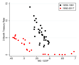
Figure 15: Money demand for M2 and its components

Table 8: Cointegration regressions and tests (M2)

Dependent Variable:	$ln(m_{t})$		$ln(d_{t})$
	OLS	CCR	OLS	CCR
	(1)	(2)	(3)	(4)
$r_{t}$	$0.009^{***}$	$-0.019^{***}$	$0.013^{***}$	$-0.020^{***}$
	(0.002)	(0.002)	(0.002)	(0.003)
$ln(uc_{t})$		$-0.182^{***}$		$-0.225^{***}$
		(0.024)		(0.027)
$adjR^{2}$	0.133	0.306	0.201	0.288
$N$	112	112	112	112
Johansen $r=0$	18.582	40.396	19.210	39.421
5% Critial Value for $r=0$	15.41	29.68	15.41	29.68
1% Critial Value for $r=0$	20.04	35.65	20.04	35.65
Johansen $r=1$	2.762	13.177	2.713	13.364
5% Critial Value for $r=1$	3.76	15.41	3.76	15.41
1% Critial Value for $r=1$	6.65	20.04	6.65	20.04

Notes: Columns (1) and (3) report OLS estimates and columns (2) and (4) report the canonical cointegrating regression (CCR) estimates. First-stage long-run variance estimation for CCR is based on Bartlett kernel and lag 1. For (1) and (2) Newey-West standard errors with lag 1 are reported in parentheses. Intercepts are included but not reported. ***, **, and * denote significance at the 1, 5, and 10 percent levels, respectively. Johansen cointegration test results are reported in column (1)-(4). The data are quarterly from 1980Q1 to 2007Q4.

To see whether the unsecured credit can account for this breakdown in M2, I repeated the analysis of Table 1 using M2 instead of M1. Table 8 reports the results. Again, I focus on the post-1980 period, until the arrival of the Great Recession. In columns (2) and (4) the Johansen tests reject their null of no cointegration at 99 percent confidence level, suggesting there exists a stable relationship between M2 real money balances, interest rates, and real balances of unsecured credit. The canonical cointegrating regression estimates in columns (2) and (4) show that the estimated coefficients on $r_{t}$ and $ln(uc_{t})$ both are negative and significantly different from zero. Thus, using the cointegrating regressions and tests, I document the evidence that once we account for the substitution effect of consumer credit, there still exists a stable negative relationship between M2 real balances and the interest rates.

Table 9 provides the unit root test results for M2 to output ratio and deposit component of the M2 to output ratio. For all the two variables, the unit root tests fail to reject the null hypothesis of non-stationarity while their first differences reject the null hypothesis of non-stationarity at 1% significance level. All series are demeaned before implementing the unit root test

Table 9: Unit root test (M2)

	Phillips-Perron test
	$Z(\rho)$	$Z(t)$
$ln(m)$	$0.567$	$0.297$
$ln(d)$	$1.275$	$1.054$
$\Delta ln(m)$	$-46.623^{***}$	$-5.335^{***}$
$\Delta ln(d)$	$-42.267^{***}$	$-5.060^{***}$

Notes: All series are demeaned before implementing the unit root test because the magnitude of the initial value can be problematic, as pointed out by Elliott and Müller (2006) and Harvey et al. (2009). ***, **, and * denote significance at the 1, 5, and 10 percent levels, respectively.

Appendix C Quantitative Robustness

C.1 Robustness I: Different Measure of Monetary Policy

Different papers have used different series as monetary instruments. For example, Lucas (2000) and Lagos and Wright (2005) use commercial paper rate. Bethune et al. (2020) uses 3 month treasury bill rate. New Keynesian literature usually use federal funds rate (e.g, Christiano, Eichenbaum and Evans, 2005 Smets and Wouters, 2007, Christiano, Eichenbaum and Trabandt, 2016) or 3 month treasury bill rate (e.g., Ireland, 2011) as measure of monetary policy while those models don’t fit to the money demand. This section checks the robustness of the main quantitative results by using different measures of monetary policy: commercial paper rate, and federal funds rate.

Table 10: Parametrizations with different measure of monetary policy

Interest	3 Month T-bill		CP		Federal Funds
	Data	Model	Data	Model	Data	Model
Targets
avg. retail markup	1.384	1.384	1.384	1.384	1.384	1.388
avg. $C/Y$	0.044	0.044	0.044	0.044	0.044	0.043
avg. $R/Y$	0.014	0.017	0.014	0.017	0.014	0.017
avg. $C/D$	0.529	0.520	0.529	0.520	0.529	0.512
avg. $UC/DM$	0.387	0.370	0.387	0.370	0.387	0.371
avg. $\Pi/Y$	0.0016	0.0011	0.0016	0.0011	0.0016	0.0011
semi-elasticity of $C/Y$	-3.716	-3.724	-3.713	-3.712	-3.020	-3.719

• Note: $C$, $R$, $DM$, $UC$, $Y$ denote currency in circulation, reserves, DM transactions, unsecured credit and nominal GDP, respectively.

Table 10 compares how model moments change depending on different measures of monetary policy. The table shows that the results are not very sensitive because the model matches the target moments well, even when different measures of monetary policy are used. Figure 16 compares the model fits using different measures of monetary policy. The model-generated series also show similar patterns for the M1 money multiplier, the excess reserve ratio, and the currency deposit ratio.

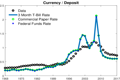
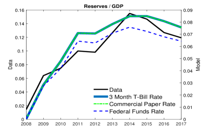
Figure 16: Model fit with different measure of monetary policy

C.2 Robustness II: Other Specifications

This section summarizes alternative parameterization results. For robustness, I examine how results are sensitive with respect to different parameter for curvature parameter for deposit operating cost while keeping other parameters are same. For Model 1, I set $\gamma(\tilde{d})=A\tilde{d}^{1.15}$ while I set $\gamma(\tilde{d})=A\tilde{d}^{1.25}$ in the Model 2.

Table 11 compares how model moments change depending on different parameterization. The table shows that the results are not very sensitive depending on different parameterizations. Figure 17 compares the model fits under different parameterizations. The model-generated series also show similar patterns for the M1 money multiplier, the excess reserve ratio, and the currency deposit ratio.

Table 11: Alternative parametrizations

	Data	Baseline	Model 1	Model 2
External Parameters
$a$		1.2	1.15	1.25
$\sigma_{3}$		0.69	0.69	0.69
Calibration targets
avg. retail markup	1.384	1.384	1.384	1.384
avg. $C/Y$	0.044	0.044	0.044	0.044
avg. $R/Y$	0.014	0.017	0.017	0.017
semi-elasticity of $C/Y$	-3.713	-3.712	-3.712	-3.712
avg. $C/D$	0.529	0.520	0.520	0.520
avg. $UC/DM$	0.387	0.370	0.370	0.370
avg. $\Pi/Y$	0.0016	0.0011	0.0011	0.0011

• Note: $C$, $R$, $DM$, $UC$, $Y$ denote currency in circulation, reserves, DM transactions, unsecured credit and nominal GDP, respectively.

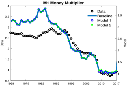
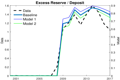
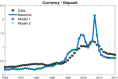
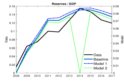
Figure 17: Model fit with different specifications

Appendix D Data Sources and Variable Definitions

• Federal funds rates: “Effective Federal Funds Rate” (FRED series FEDFUNDS).

• Interest on reserves: “Interest Rate on Excess Reserves” (FRED series IOER) and “Interest Rate on Required Reserves” (FRED series IORR).

• 3-month treasury rate: “3-Month Treasury Bill: Secondary Market Rate” (FRED series TB3MS).

• Deposit / Total checkable deposits: “Total Checkable Deposits” (FRED series TCDSL).

• Excess reserves: “Excess Reserves of Depository Institutions” (FRED series EXCRESNS) and (FRED series EXCSRESNS).

• Excess reserve ratio: $\frac{\text{Excess reserves}}{\text{Total checkable deposits}}$.

• Required reserves: “Required Reserves of Depository Institutions” (FRED series REQRESNS).

• Required reserves ratio: $\frac{\text{Required reserves}}{\text{Total checkable deposits}}$.

• Reserves: “Total Reserves of Depository Institutions” (FRED series TOTRESNS).

• M1: “M1 Money Stock” (FRED series M1SL).

• M2: “M2 Money Stock” (FRED series M2SL).

• Monetary base: “Monetary Base; Total” (FRED series BOGMBASE).

• M1 money multiplier: $\frac{\text{M1}}{\text{Monetary Base}}$.

• Currency: “Currency Component of M1” (FRED series CURRSL).

• Deposit Component of M1: M1$-$Currency.

• Deposit Component of M2: M2$-$Currency.

• Unsecured credit: “Revolving Consumer Credit Owned and Securitized” (FRED series REVOLSL) transformed from monthly to quarterly by summing monthly data.

• GDP: “Gross Domestic Product” (FRED series GDP), quarterly and “Gross Domestic Product” (FRED series GDPA), annual.

• Commercial paper rate: “Nominal interest rate” from Ireland (2009), updated to 2017 using “3-Month AA Nonfinancial Commercial Paper Rate” (FRED series CPN3M).

The quantitative analysis uses the annual average of above series.

References

- (1)
- Afonso and Lagos (2015) Afonso, Gara and Ricardo Lagos, “Trade Dynamics in the Market for Federal Funds,” Econometrica, 2015, 83 (1), 263–313.
- Afonso et al. (2019) , Roc Armenter, and Benjamin Lester, “A Model of the Federal Funds Market: Yesterday, Today, and Tomorrow,” Review of Economic Dynamics, 2019, 33, 177–204.
- Altermatt (2019) Altermatt, Lukas, “Bank Lending, Financial Frictions, and Inside Money Creation,” University of Zurich, Department of Economics, Working Paper No. 325, 2019.
- Andolfatto et al. (2020) Andolfatto, David, Aleksander Berentsen, and Fernando M Martin, “Money, Banking, and Financial Markets,” The Review of Economic Studies, 2020, 87 (5), 2049–2086.
- Armenter and Lester (2017) Armenter, Roc and Benjamin Lester, “Excess Reserves and Monetary Policy Implementation,” Review of Economic Dynamics, 2017, 23, 212–235.
- Bech and Klee (2011) Bech, Morten L and Elizabeth Klee, “The Mechanics of a Graceful Exit: Interest on Reserves and Segmentation in the Federal Funds Market,” Journal of Monetary Economics, 2011, 58 (5), 415–431.
- Berentsen et al. (2007) Berentsen, Aleksander, Gabriele Camera, and Christopher Waller, “Money, Credit and Banking,” Journal of Economic Theory, 2007, 135 (1), 171–195.
- Berentsen et al. (2015) , Samuel Huber, and Alessandro Marchesiani, “Financial Innovations, Money Demand, and the Welfare Cost of Inflation,” Journal of Money, Credit and Banking, 2015, 47 (S2), 223–261.
- Bethune et al. (2020) Bethune, Zachary, Michael Choi, and Randall Wright, “Frictional Goods Markets: Theory and Applications,” The Review of Economic Studies, 2020, 87 (2), 691–720.
- Bianchi and Bigio (2014) Bianchi, Javier and Saki Bigio, “Banks, Liquidity Management and Monetary Policy,” NBER Working Paper No. 20490, September 2014.
- Cagan (1956) Cagan, Phillip, “The Monetary Dynamics of Hyperinflation,” Studies of the Quantity Theory if Money, 1956.
- Chiu et al. (2020) Chiu, Jonathan, Jens Eisenschmidt, and Cyril Monnet, “Relationships in the Interbank Market,” Review of Economic Dynamics, 2020, 35, 170–191.
- Christiano et al. (2005) Christiano, Lawrence J, Martin Eichenbaum, and Charles L Evans, “Nominal Rigidities and the Dynamic Effects of a Shock to Monetary Policy,” Journal of Political Economy, 2005, 113 (1), 1–45.
- Christiano et al. (2016) , Martin S Eichenbaum, and Mathias Trabandt, “Unemployment and Business Cycles,” Econometrica, 2016, 84 (4), 1523–1569.
- Cochrane (2014) Cochrane, John H, “Monetary Policy with Interest on Reserves,” Journal of Economic Dynamics and Control, 2014, 49, 74–108.
- Curdia and Woodford (2011) Curdia, Vasco and Michael Woodford, “The Central-Bank Balance Sheet as an Instrument of Monetary Policy,” Journal of Monetary Economics, 2011, 58 (1), 54–79.
- Elliott and Müller (2006) Elliott, Graham and Ulrich K Müller, “Minimizing the Impact of the Initial Condition on Testing for Unit Roots,” Journal of Econometrics, 2006, 135 (1-2), 285–310.
- Ennis (2018) Ennis, Huberto M, “A Simple General Equilibrium Model of Large Excess Reserves,” Journal of Monetary Economics, 2018, 98, 50–65.
- Feinman (1993) Feinman, Joshua N, “Reserve Requirements: History, Current Practice, and Potential Reform,” Federal Reserve Bulletin, 1993, 79, 569.
- Freeman (1987) Freeman, Scott, “Reserve Requirements and Optimal Seigniorage,” Journal of Monetary Economics, 1987, 19 (2), 307–314.
- Freeman and Kydland (2000) and Finn E Kydland, “Monetary Aggregates and Output,” American Economic Review, 2000, 90 (5), 1125–1135.
- Freeman and Huffman (1991) and Gregory W Huffman, “Inside Money, Output, and Causality,” International Economic Review, 1991, pp. 645–667.
- Gu et al. (2016) Gu, Chao, Fabrizio Mattesini, and Randall Wright, “Money and Credit Redux,” Econometrica, 2016, 84 (1), 1–32.
- Gu et al. (2013) , , Cyril Monnet, and Randall Wright, “Banking: A New Monetarist Approach,” Review of Economic Studies, 2013, 80 (2), 636–662.
- Harvey et al. (2009) Harvey, David I, Stephen J Leybourne, and AM Robert Taylor, “Unit Root Testing in Practice: Dealing with Uncertainty over the Trend and Initial Condition,” Econometric Theory, 2009, 25 (3), 587–636.
- Haslag and Young (1998) Haslag, Joseph H and Eric R Young, “Money Creation, Reserve Requirements, and Seigniorage,” Review of Economic Dynamics, 1998, 1 (3), 677–698.
- Ireland (2009) Ireland, Peter N, “On the Welfare Cost of Inflation and the Recent Behavior of Money Demand,” American Economic Review, 2009, 99 (3), 1040–52.
- Ireland (2011) , “A New Keynesian Perspective on the Great Recession,” Journal of Money, Credit and Banking, 2011, 43 (1), 31–54.
- Kashyap and Stein (2012) Kashyap, Anil K and Jeremy C Stein, “The Optimal Conduct of Monetary Policy with Interest on Reserves,” American Economic Journal: Macroeconomics, 2012, 4 (1), 266–82.
- Keister et al. (2008) Keister, Todd, Antoine Martin, and James McAndrews, “Divorcing Money from Monetary Policy,” Economic Policy Review, 2008, 14 (2).
- Krueger and Perri (2006) Krueger, Dirk and Fabrizio Perri, “Does Income Inequality Lead to Consumption Inequality? Evidence and Theory,” The Review of Economic Studies, 2006, 73 (1), 163–193.
- Lagos and Wright (2005) Lagos, Ricardo and Randall Wright, “A Unified Framework for Monetary Theory and Policy Analysis,” Journal of Political Economy, 2005, 113 (3), 463–484.
- Lee (2016) Lee, Seungduck, “Money, Asset Prices, and the Liquidity Premium,” Journal of Money, Credit and Banking, 2016.
- Lester et al. (2012) Lester, Benjamin, Andrew Postlewaite, and Randall Wright, “Information, Liquidity, Asset Prices, and Monetary Policy,” The Review of Economic Studies, 2012, 79 (3), 1209–1238.
- Lotz and Zhang (2016) Lotz, Sebastien and Cathy Zhang, “Money and Credit as Means of Payment: A New Monetarist Approach,” Journal of Economic Theory, 2016, 164, 68–100.
- Lucas (2000) Lucas, Robert E, “Inflation and Welfare,” Econometrica, 2000, pp. 247–274.
- Lucas and Nicolini (2015) and Juan Pablo Nicolini, “On the Stability of Money Demand,” Journal of Monetary Economics, 2015, 73, 48–65.
- Nakamura (2018) Nakamura, Emi, “Discussion of Monetary Policy: Conventional and Unconventional,” May 2018. Nobel Symposium, Swedish House of Finance.
- Park (1992) Park, Joon Y, “Canonical Cointegrating Regressions,” Econometrica: Journal of the Econometric Society, 1992, pp. 119–143.
- Rocheteau et al. (2018a) Rocheteau, Guillaume, Randall Wright, and Cathy Zhang, “Corporate Finance and Monetary Policy,” American Economic Review, 2018, 108 (4-5), 1147–1186.
- Rocheteau et al. (2018b) , , and Sylvia Xiaolin Xiao, “Open Market Operations,” Journal of Monetary Economics, 2018, 98, 114–128.
- Sanches and Williamson (2010) Sanches, Daniel and Stephen Williamson, “Money and Credit with Limited Commitment and Theft,” Journal of Economic Theory, 2010, 145 (4), 1525–1549.
- Sargent and Wallace (1982) Sargent, Thomas J and Neil Wallace, “The Real-Bills Doctrine versus the Quantity Theory: A Reconsideration,” Journal of Political Economy, 1982, 90 (6), 1212–1236.
- Smets and Wouters (2007) Smets, Frank and Rafael Wouters, “Shocks and Frictions in US Business Cycles: A Bayesian DSGE Approach,” American Economic Review, 2007, 97 (3), 586–606.
- Teles and Zhou (2005) Teles, Pedro and Ruilin Zhou, “A Stable Money Demand: Looking for the Right Monetary Aggregate,” Economic Perspectives, 2005, 29 (1), 50.
- VanHoose and Humphrey (2001) VanHoose, David D and David B Humphrey, “Sweep accounts, Reserve Management, and Interest Rate Volatility,” Journal of Economics and Business, 2001, 53 (4), 387–404.
- Williamson (2016) Williamson, Stephen D, “Scarce Collateral, the Term Premium, and Quantitative Easing,” Journal of Economic Theory, 2016, 164, 136–165.
- Williamson et al. (2019) Williamson, Stephen et al., “Central Bank Digital Currency: Welfare and Policy Implications,” 2019 Meeting Papers No. 386, 2019. Society for Economic Dynamics.