Analytic one-dimensional maps and two-dimensional ordinary differential equations can robustly simulate Turing machines

Abstract

In this paper, we analyze the problem of finding the minimum dimension $n$ such that a closed-form analytic map/ordinary differential equation can simulate a Turing machine over $\mathbb{R}^{n}$ in a way that is robust to perturbations. We show that one-dimensional closed-form analytic maps are sufficient to robustly simulate Turing machines; but the minimum dimension for the closed-form analytic ordinary differential equations to robustly simulate Turing machines is two, under some reasonable assumptions. We also show that any Turing machine can be simulated by a two-dimensional $C^{\infty}$ ordinary differential equation on the compact sphere $\mathbb{S}^{2}$.

1 Introduction

As it is well known (see e.g. [Sip12]), a Turing machine is a mathematical model of computation that formalizes the notion of algorithm/computation over discrete structures such as the set of positive integers $\mathbb{N}$ or integers $\mathbb{Z}$. In practice, Turing machines are computationally equivalent to a standard digital computer. Furthermore, following the work of Turing and others it is also known that some problems such as the Halting Problem or Hilbert’s 10th problem are noncomputable, i.e. there is no Turing machine (i.e. no algorithm) that solves those problems [Tur37], [Mat93]. This remarkable result shows that some problems are algorithmically unsolvable. Examples of other nontrivial behavior regarding Turing machines include, for instance, the existence of universal Turing machines, which can simulate the computation of any other Turing machine (see [Tur37] or e.g. [Sip12]), or the existence of self-reproducing Turing machines which output their own description [Mos10].

Although the results above are considered classically over discrete structures (e.g. $\mathbb{N}$), often they can be studied over continuous spaces such as $\mathbb{R}^{n}$. The idea is to simulate the computation of a Turing machine with a continuous map/flow. If a continuous system is able to simulate any Turing machine (or, equivalently, a universal Turing machine), then this system is usually referred to as Turing universal. A consequence of the noncomputability of the Halting Problem is that the long term behavior of Turing universal systems is highly complex (in a manner distinct from behaviors considered e.g. in chaos theory) and has some characteristics which are not computable (see e.g. [Moo91]). However, in applications, it is often desirable that Turing universal systems are relatively simple and mathematically well-behaved so that they can be used in meaningful situations. For this reason, one might be interested in having properties such as low-dimensionality, reasonable smoothness, or robustness to perturbations for Turing universal systems.

In this paper, we investigate the problem of determining the lowest dimension $n$ such that the analytic maps/ODEs defined on $\mathbb{R}^{n}$ can robustly simulate Turing machines.

It is well-known that piecewise affine and other types of maps and ODEs can simulate Turing machines on $\mathbb{R}^{n}$, see e.g. [Moo91], [KCG94], [Bra95], [Koi96], [Bou99], [KP05], [BC08], [BP21]). However, some authors have claimed (see e.g. [MO98], [KM99], [AB01], [KM99], [BGH13]) that, when focusing on more physically realistic systems simulating Turing machines, one might desire other additional attributes such as robustness to noise (it is known that the addition of noise to some classes of systems reduces their computational power, see e.g. [MO98], [AB01]) or smoothness of the dynamics since most classical physical systems are expressed with smooth (actually analytic) functions. In [KM99] the authors have shown that closed-form analytic maps (i.e. those analytic functions which can be expressed in terms of elementary functions such as polynomials, trigonometric functions, exponential and logarithmic functions, their composition, etc.) are capable of simulating Turing machines with exponential slowdown in dimension one or in real time in dimension $\geq 2$. In [GCB08] it was shown that, under a certain notion of robustness (see Theorems 1 and 3 below), the class of closed-form analytic maps on $\mathbb{R}^{3}$ as well as the class of ODEs defined with analytic closed-form functions in $\mathbb{R}^{6}$ can robustly simulate Turing machines.

In the present paper, we show that one-dimensional closed-form analytic maps can robustly simulate Turing machine on $\mathbb{R}$ (Theorem 9) in real time (i.e. without the exponential slowdown of [KM99]; the simulation in [KM99] is not robust to perturbations either) and that two-dimensional closed-form analytic ODEs can also robustly simulate Turing machines (Theorem 11), both in the sense of [GCB08]. We also show that, under certain reasonable assumptions, none of one-dimensional autonomous analytic ODEs can simulate (robustly or not) a universal Turing machine.

Similar to what is done in [CMPS21], we show that there is a $C^{\infty}$ ODE which can simulate Turing machines over the compact set $\mathbb{S}^{n}=\{x\in\mathbb{R}^{n+1}:\left\|x\right\|=1\}$ for $n\geq 2$. The difference between our result and the result of [CMPS21] is that, although the flow of [CMPS21] is mathematically simpler (it is polynomial), Turing universality is only achieved over $\mathbb{S}^{n}$ for $n\geq 17$. The authors then use this polynomial flow to construct a (Euler) partial differential equation which is Turing universal. We also note that in [CMPSP21] the authors proved that there are Turing complete (stationary Euler) fluid-flows on a Riemannian 3-dimensional sphere. The difference of the later result from the one presented in this paper is that we use ODEs instead of partial differential equations, and our results are for $\mathbb{S}^{2}$ instead of $\mathbb{S}^{3}$.

The outline of the paper is as follows. In Section 2 we review the construction presented in [GCB08] to create analytic maps on $\mathbb{R}^{3}$ which can robustly simulate Turing machines. In Section 3 we present some auxiliary functions. Building on these results, we show in Section 4 that one-dimensional analytic maps can robustly simulate Turing machines. By iterating these maps with ODEs, we are able to show in Section 5 that two-dimensional ODEs can robustly simulate Turing machines. In Section 6, we construct a $C^{\infty}$ ODE that can simulate Turing machines over the compact set $\mathbb{S}^{2}$. Finally, in Section 7 we show that under reasonable hypothesis, no one-dimensional analytic ODE can simulate a universal Turing machine.

2 Simulating Turing machines in dimension three

In this section, we review several results from [GCB08] which are useful for proving our main results.

We first recall some basic results from computability theory (see e.g. [Sip12]). Given a finite set $\Sigma$ (the alphabet), a word over $\Sigma$ is a finite sequence $w=(w_{1},...,w_{k})\in\Sigma^{k}$ for some $k\in\mathbb{N}_{0}$ ($k$ is the length of the word), where $\mathbb{N}_{0}$ is the set of all non-negative integers. Note that there is a special sequence, represented by $\epsilon$, which denotes the word of length $0$. As usual, for notational simplicity, we will denote the word $w=(w_{1},...,w_{k})$ simply as $w=w_{1}...w_{k}$. The set of all words over $\Sigma$ is denoted by $\Sigma^{\ast}$. We also recall that a Turing machine is a discrete dynamical system defined by the iteration of a map, although it is usually viewed as a finite-state machine since this approach is often more convenient. More specifically, let $\Sigma$ be an alphabet, and take some symbol $B\notin\Sigma$, which is usually known as the blank symbol, and let $Q$ be a finite set known as the set of states with some special elements $q_{0},q_{h}\in Q$, called the initial state and the final state, respectively. Then a Turing machine $M$ is a map $F_{M}:\Sigma^{\ast}\times\Sigma^{\ast}\times Q\rightarrow\Sigma^{\ast}\times\Sigma^{\ast}\times Q$ that works as follows when viewed as a machine. It has a bi-infinite tape, divided into cells, and a head which is associated to some state of $Q$. Given some $(u,v,q)\in\Sigma^{\ast}\times\Sigma^{\ast}\times Q$ (the configuration of the Turing machine), where $u=u_{1}u_{2}\ldots u_{n}$ and $v=v_{1}v_{2}\ldots v_{p}$, then the tape contents of the Turing machine at this configuration is

$$...B\,B\,B\,v_{p}...\,v_{2}v_{1}\,u_{1}u_{2}\ldots u_{n}\,B\,B\,B...,$$ (1)

while its associated state is $q$. In this case the Turing machine is also said to be reading symbol $v_{1}$. Then, depending only on the value of the current state and of the symbol being read by the head, the machine simultaneously (i) updates its state, (ii) updates the symbol being read by the head and (iii) either moves the head one cell to the right, one cell to the left, or maintains the head on the same position.

A Turing machine $M$ computes a function $f:\Sigma^{\ast}\rightarrow\Sigma^{\ast}$ as follows. Given a word $w$ it starts its computation on the initial configuration $(w,\epsilon,q_{0})$, i.e. in the initial configuration the state is the initial state and the tape contains the input $w$ only. Then $M$ proceeds with the computation until it reaches the halting state $q_{h}$. In this case we say that the Turing machine has halted with configuration $(u_{h},v_{h},q_{h})\in\Sigma^{\ast}\times\Sigma^{\ast}\times Q$. In this case its output will be $u_{h}$, i.e. $u_{h}=f(w)$. If $M$ does not halt with input $w$, then $f(w)$ is undefined.

Given some Turing machine $M$ as described above, let $k=1+\#\Sigma$ and take an injective map $\gamma:\Sigma\rightarrow\{0,1,2,\ldots,k-1\}$ with $\gamma(B)=0$. Let $(u,v,q)$ be the current configuration of $M$ and let us further assume that $M$ has $m$ states, represented by the numbers $1,\ldots,m$, and that if $M$ reaches an halting configuration, then it moves to the same configuration (i.e.$\ F_{M}(u_{h},v_{h},q_{h})=(u_{h},v_{h},q_{h})$). Take

$$\begin{array}[c]{l}y_{1}=\gamma(u_{1})+\gamma(u_{2})k+\ldots+\gamma(u_{n})k^{n-1}\\ y_{2}=\gamma(v_{1})+\gamma(v_{2})k+\ldots+\gamma(v_{p})k^{p-1}\end{array}$$ (2)

and suppose that $q$ is the state associated to the current configuration. Then $(y_{1},y_{2},q)\in\mathbb{N}^{3}$ encodes unambiguously the current configuration of $M$. Under these assumptions, the transition function of $M$ can be encoded as a function $\bar{f}_{M}:\mathbb{N}^{3}\rightarrow\mathbb{N}^{3}$. In [GCB08] it was shown that $\bar{f}_{M}$ can be extended to a function $f_{M}:\mathbb{R}^{3}\rightarrow\mathbb{R}^{3}$, which has the following properties: (i) it is capable of simulating $M$ in the presence of perturbations; (ii) the function $f$ is analytic, and each of its components can be expressed using only the following terms: variables, polynomial-time computable constants (see Remark 2 for a definition), $+$, $-$, $\times$, $\sin$, $\cos$, $\arctan$. The precise statement of this result is given below, where $\left\|f\right\|=\sup_{x\in A}\left\|f(x)\right\|$ for a function $f:A\subseteq\mathbb{R}^{l}\rightarrow\mathbb{R}^{j}$, $\left\|y\right\|=\max_{1\leq i\leq j}\left|y_{i}\right|$ for $y=(y_{1},\ldots,y_{j})\in\mathbb{R}^{j}$, and $f^{[k]}$ denotes the $k$th iterate of the function $f:A\rightarrow A$, which is defined as follows: $f^{[0]}(x)=x$, $f^{[k+1]}(x)=f^{[k]}(f(x))$.

Theorem 1 ([GCB08, p. 333])

Let $\psi:\mathbb{N}^{3}\rightarrow\mathbb{N}^{3}$ be the transition function of a Turing machine $M$ under the encoding described above, and let $0<\delta<\varepsilon<1/2$. Then $\psi$ admits a globally analytic closed-form extension $f_{M}:\mathbb{R}^{3}\rightarrow\mathbb{R}^{3}$ such that the expression of each component of $f_{M}$ can be written using only the following terms: variables, polynomial-time computable constants, $+$, $-$, $\times$, $\sin$, $\cos$, $\arctan$. Moreover, $f_{M}$ is robust to perturbations in the following sense: for all $f$ such that $\left\|f-f_{M}\right\|\leq\delta$, for all $j\in\mathbb{N}$, and for all $\bar{x}_{0}\in\mathbb{R}^{3}$ satisfying $\left\|\bar{x}_{0}-x_{0}\right\|\leq\varepsilon,$ where $x_{0}\in\mathbb{N}^{3}$ represents a configuration according to the encoding described above,

$$\left\|f^{[j]}(\bar{x}_{0})-\psi^{[j]}(x_{0})\right\|\leq\varepsilon.$$

We note that the proof of this theorem is constructive and that $f_{M}$ can be obtained explicitly. A continuous-time version of Theorem 1 was also proved in [GCB08].

Remark 2

We note that we can define computable real constants and computable real functions using the approach of computable analysis. These notions can be presented in several equivalent but different ways. For example, according to the approach presented in [Ko91] (see also [BHW08]), a number $c\in\mathbb{R}$ is computable if there is a Turing machine $M$ that, on input $n\in\mathbb{N}$, outputs (in finite time) a rational $q_{n}$ with the property that $\left|q_{n}-c\right|\leq 2^{-n}$. If the Turing machine $M$ runs in polynomial time (in $n$), then we say that $c$ is computable in polynomial time. Similarly, a function $f:\mathbb{R\rightarrow R}$ is computable if there is an oracle Turing machine $M$ that computes $f(x)$ in the sense that, given as input $n\in\mathbb{N}$ and any oracle $\varphi:\mathbb{N}\to\mathbb{Q}$ recording $x\in\mathbb{R}$ (i.e. with the property that $\left|x-\varphi(n)\right|\leq 2^{-n}$), $M$ outputs a rational number $q_{n}$ such that $\left|q_{n}-c\right|\leq 2^{-n}$. A $C^{1}$ real function $f:\mathbb{R\rightarrow R}$ is $C^{1}$-computable if $f$ and its derivative are both computable. These notions can be generalized to $\mathbb{R}^{n}$ in a straightforward manner.

Theorem 3 ([GCB08, p. 333])

Let $\psi:\mathbb{N}^{3}\rightarrow\mathbb{N}^{3}$ be the transition function of a Turing machine $M$ under the encoding described above; let $0<\varepsilon\leq 1/4$; and let $0\leq\delta<2\varepsilon\leq 1/2$. Then there exist

• $\eta>0$ satisfying $\eta<1/2$, which can be computed from $\psi,\varepsilon,\delta$, and

• an analytic closed-form function $g_{M}:\mathbb{R}^{7}\rightarrow\mathbb{R}^{6}$ which can be written using only the following terms: variables, polynomial-time computable constants, $+$, $-$, $\times$, $\sin$, $\cos$, $\arctan$

such that the ODE $z^{\prime}=g_{M}(t,z)$ robustly simulates $M$ in the following sense: for all $g$ satisfying $\left\|g-g_{M}\right\|\leq\delta<1/2$ and for every $x_{0}\in\mathbb{N}^{3}$ that encodes a configuration according to the encoding described above, if $\bar{x}_{0},\bar{y}_{0}\in\mathbb{R}^{3}$ satisfy the conditions $\left\|\bar{x}_{0}-x_{0}\right\|\leq\varepsilon$ and $\left\|\bar{y}_{0}-x_{0}\right\|\leq\varepsilon$, then the solution $z(t)$ of

$$z^{\prime}=g(t,z),\qquad z(0)=(\bar{x}_{0},\bar{y}_{0})$$

satisfies, for all $j\in\mathbb{N}$ and for all $t\in[j,j+1/2]$,

$$\left\|z_{2}(t)-\psi^{[j]}(x_{0})\right\|\leq\eta,$$ (3)

where $z\equiv(z_{1},z_{2})$, with $z_{1}\in\mathbb{R}^{3}$ and $z_{2}\in\mathbb{R}^{3}$.

3 Some useful auxiliary functions

In this section we present several functions and results which are needed in subsequent sections. The function $\Upsilon$ presented in the next lemma can be seen as a generalization of the error-correcting function $l_{2}$ from [GCB08, Lemma 9]. More specifically, the function $\Psi$ can be viewed as a function that improves the accuracy of approximations within distance $\leq 1/5$ of an integer (the function $l_{2}$ of [GCB08, Lemma 9] has a similar property, but only works for the integers $0$ and 1$)$, where the correction factor is bounded by $e^{-y}$, and $y>0$ is the second argument of $\Psi$.

Lemma 4

Let $\Psi:\mathbb{R}^{2}\rightarrow\mathbb{R}$ be given by $\Psi(x,y)=x-\frac{1}{2\pi}\arcsin(\sin(2\pi x)(1-e^{-y-2})).$ Then $\left|\Psi(x,y)-k\right|<e^{-y}\left|x-k\right|$ whenever $\left|x-k\right|\leq 1/5$ for some $k\in\mathbb{Z}$ and $y\geq 0$.

Proof. Let $\overline{\Psi}:\mathbb{R}\rightarrow\mathbb{R}$ be defined by $\overline{\Psi}(x)=x-\frac{1}{2\pi}\arcsin(\sin(2\pi x))$. We note that, since $\sin(2\pi x)$ has period 1, $\overline{\Psi}(x)=k$ if $x\in[k-1/4,k+1/4]$ for some $k\in\mathbb{Z}$. However, although it is continuous, the function $\overline{\Psi}$ is not analytic, since it is well-known that if an analytic function is constant in a non-empty interval, e.g. $[3/4,5/4]$, then it should be constant everywhere on the real line $\mathbb{R}$, which is not the case for $\overline{\Psi}$. The problem is that, although the composition of analytic functions yields again an analytic function, the derivative of $\arcsin y$ is not defined when $y=-1$ or $y=1$ and thus $\overline{\Psi}$ is not analytic when $x=k-1/4$ or $x=k+1/4$ for some $k\in\mathbb{Z}$. Note, however, that $\arcsin$ is analytic in $(-1,1)$. Hence, we can multiply $\sin(2\pi x)$ by a value $1-e^{-y}$ (or $1-e^{-y-2}$, which will be more convenient later on), which is slightly less than 1, to ensure that the resulting function $\Psi$ is analytic, since in this way we guarantee that $-1<\sin(2\pi x)(1-e^{-y})<1$ for any $x\in\mathbb{R}$ and $y\geq 0$. Next we notice that, by the mean value theorem

$$\left|\arcsin a-\arcsin b\right| \leq\left|a-b\right|\max_{x\in[a,b]}\frac{1}{\sqrt{1-x^{2}}}$$

$$=\left|a-b\right|\max\left(\frac{1}{\sqrt{1-a^{2}}},\frac{1}{\sqrt{1-b^{2}}}\right).$$

Let us now take $g(x)=7x-\sin(2\pi x)$. We note that $g(0)=0$ and that $g^{\prime}(x)=7-2\pi\cos(2\pi x)>0$. Hence we conclude that $g$ strictly increases in $[0,1/5]$, which implies $7\left|x\right|\geq\left|\sin(2\pi x)\right|$ when $x\in[-1/5,1/5]$. This implies that for $x\in[k-1/5,k+1/5]$, where $k\in\mathbb{Z}$ is arbitrary, we have

$$\left|\Psi(x,y)-k\right| =\left|x-\frac{1}{2\pi}\arcsin(\sin(2\pi x)(1-e^{-y-2}))-\left(x-\frac{1}{2\pi}\arcsin(\sin(2\pi x))\right)\right|$$

$$=\frac{1}{2\pi}\left|\arcsin(\sin(2\pi x))-\arcsin(\sin(2\pi x)(1-e^{-y-2}))\right|$$

$$\leq\frac{1}{2\pi}\frac{1}{\sqrt{1-\sin^{2}(2\pi/5)}}\left|\sin\left(2\pi x\right)(1-(1-e^{-y-2}))\right|$$

$$=\frac{1}{2\pi}\frac{1}{\sqrt{1-\sin^{2}(2\pi/5)}}\left|\sin\left(2\pi(x-k)\right)\right|e^{-y-2}$$

$$<\left|\sin\left(2\pi(x-k)\right)\right|e^{-y}e^{-2}$$

$$\leq 7\left|x-k\right|e^{-y}e^{-2}$$

$$\leq\left|x-k\right|e^{-y}.$$

 

We now present another error-correcting function $\sigma:\mathbb{R\rightarrow R}$ which was first presented in [GCB08, Proposition 5]. This function is a uniform contraction around integers. Unlike $\Psi$, one cannot prescribe the amount of error reduction around each integer with a single application of the map $\sigma$. On the other hand its use is not restricted to a $1/5$ -neighborhood of integers and can be used on larger neighborhoods. This last property will be handy later on.

Lemma 5 ([GCB08])

Let $\sigma:\mathbb{R\rightarrow R}$ be the function defined by $\sigma(x)=x-0.2\sin(2\pi x)$. Let $\varepsilon\in[0,1/2).$ Then there is some contracting factor $\lambda_{\varepsilon}\in(0,1)$ such that, $\forall\delta\in[-\varepsilon,\varepsilon],$ $\forall n\in\mathbb{Z}$, $|\sigma(n+\delta)-n|<\lambda_{\varepsilon}\delta.$

The constants $\lambda_{\varepsilon}$ can usually be explicitly obtained. For example, as shown in [GCB08], we can take $\lambda_{1/4}=0.4\pi-1\approx 0.2566371$.

It is well known that there are bijective functions from $\mathbb{N}^{2}$ to $\mathbb{N}$. An example (see e.g. [Odi89, pp. 26–27]) is the dovetailing pairing map $I:\mathbb{N}^{2}\mathbb{\rightarrow N}$ defined by the formula

$$I(x,y)=\frac{(x+y)^{2}+3x+y}{2}.$$ (4)

Using this map we can obtain a bijective map $I_{k}:\mathbb{N}^{k}\rightarrow\mathbb{N}$, for $k\geq 2$, by defining $I_{k}$ recursively: $I_{2}(x_{1},x_{2})=I(x_{1},x_{2})$; $I_{k+1}(x_{1},\ldots,x_{k},x_{k+1})=I_{2}(I_{k}(x_{1},\ldots,x_{k}),x_{k+1})$. We now show that the maps $I_{k}$ can be extended to $\mathbb{R}^{k}$ robustly around the integers. Since each $I_{k}$ is a (multivariate) polynomial, to achieve this objective we have to analyze how the error is propagated via the application of a polynomial map. The following lemma is from [BGP12], and can be viewed as an extension of a similar result proved in [GCB08, Lemma 11] for the case of monomials. For multivariate polynomials, the multi-index notation is used for compactness as follows: a monomial $x_{1}^{\alpha_{1}}\ldots x_{k}^{\alpha_{k}}$ is represented by $x^{\alpha}$, where $x=(x_{1},\ldots,x_{k})$, $\alpha=(\alpha_{1},\ldots,\alpha_{k})$, $\left|\alpha\right|=\alpha_{1}+\ldots+\alpha_{k}$ is the degree of the monomial, and the degree of a (multivariate) polynomial is the maximum degree of all the monomials which appear in its expression.

Lemma 6 ([BGP12, Lemma 4])

Let $P:\mathbb{R}^{k}\rightarrow\mathbb{R}$ be a multivariate polynomial of degree $k$ and let $x,y\in\mathbb{R}^{k}$ be such that $\left\|x\right\|,\left\|y\right\|\leq M$ for some $M\geq 0$. Then

$$\left|P(x)-P(y)\right|\leq kM^{k-1}\Sigma P\left\|x-y\right\|$$

where $\Sigma P$ denotes the sum of the absolute values of the coefficients of $P$.

Now we are ready to state the result that shows the existence of robust analytic extensions of $I_{k}$ for each $k$.

Proposition 7

For each $k\in\mathbb{N}$, $k\geq 2$, there exists an analytic function $\Upsilon_{k}:\mathbb{R}^{k}\rightarrow\mathbb{R}$ with the following properties:

1. If $x\in\mathbb{N}^{k}$, then $\Upsilon_{k}(x)=I_{k}(x)$;

2. For any $x\in\mathbb{R}^{k}$, if there is some $y\in\mathbb{N}^{k}$ such that $\left\|x-y\right\|\leq 1/5$, then $\left|\Upsilon_{k}(x)-I_{k}(y)\right|\leq\left\|x-y\right\|\leq 1/5.$

Proof. We start with the case $k=2$. Since

$$I_{2}(x_{1},x_{2})=\frac{(x_{1}+x_{2})^{2}+3x_{1}+x_{2}}{2}=\frac{x_{1}^{2}+2x_{1}x_{2}+x_{2}^{2}+3x_{1}+x_{2}}{2},$$

it is clear that the function $I_{2}$ is well-defined for all $x_{1},x_{2}\in\mathbb{R}$. In the remaining of this proof, we assume that $I_{2}$ is defined over $\mathbb{R}^{2}$. Since $I_{2}$ is a polynomial of degree 2, by Lemma 6 we conclude that

$$\left|I_{2}(x)-I_{2}(y)\right|\leq 8\max(\left\|x\right\|,\left\|y\right\|)\left\|x-y\right\|.$$

Since $\left\|x\right\|\leq 1+\left\|x\right\|^{2}$ for all $x\in\mathbb{R}^{2}$, it follows that

$$\left|I_{2}(x)-I_{2}(y)\right|\leq 8(2+\left\|x\right\|^{2}+\left\|y\right\|^{2})\left\|x-y\right\|.$$ (5)

Set

$$\Upsilon_{2}(x_{1},x_{2})=I_{2}(\Psi(x_{1},32(1+\left\|x\right\|_{2}^{2})),\Psi(x_{2},32(1+\left\|x\right\|_{2}^{2}))),$$

where $\left\|x\right\|_{2}^{2}=x_{1}^{2}+x_{2}^{2}$. As a composition of analytic functions, $\Upsilon_{2}:\mathbb{R}^{2}\rightarrow\mathbb{R}$ is clearly analytic. If $x_{1},x_{2}\in\mathbb{N}$, it is trivial to verify that $\Upsilon_{2}(x_{1},x_{2})=I_{2}(x_{1},x_{2})$, which implies property 1. For property 2, let us assume that $\left\|x-y\right\|\leq\varepsilon\leq 1/5$ for some $y\in\mathbb{N}^{k}$. Using Lemma 4 and the inequality $e^{-l}<(1/l)$ for all $l\geq 1$, we obtain the following estimate, where $\varepsilon=\left\|x-y\right\|\leq 1/5$:

$$\left\|(\Psi(x_{1},32(1+\left\|x\right\|_{2}^{2})),\Psi(x_{2},32(1+\left\|x\right\|_{2}^{2})))-(y_{1},y_{2})\right\|$$

$$\leq\varepsilon e^{-32(1+\left\|x\right\|_{2}^{2})}$$

$$\leq\frac{\varepsilon}{32(1+\left\|x\right\|_{2}^{2})}.$$ (6)

Recall that, on $\mathbb{R}^{2}$, $\|\cdot\|_{2}$ denotes the Euclidean norm while $\|\cdot\|$ denotes the maximum norm. Since $\left\|x-y\right\|\leq\frac{1}{5}$ and $\left\|y\right\|_{2}\leq\sqrt{2}\left\|y\right\|$, it follows that $\left\|x-y\right\|_{2}\leq\sqrt{2}\left\|x-y\right\|\leq 1/2$, which further implies that

$$\left\|y\right\|_{2}^{2} =\left\|y-x+x\right\|_{2}^{2}$$

$$\leq\left(\left\|x-y\right\|_{2}+\left\|x\right\|_{2}\right)^{2}$$

$$\leq\left(\frac{1}{2}+\left\|x\right\|_{2}\right)^{2}$$

$$=\frac{1}{4}+\left\|x\right\|_{2}+\left\|x\right\|_{2}^{2}$$

$$\leq\frac{1}{4}+1+\left\|x\right\|_{2}^{2}+\left\|x\right\|_{2}^{2}<2+2\left\|x\right\|_{2}^{2}\text{.}$$

Then it follows from this inequality, (5), and (6) that

$$\left|\Upsilon_{2}(x)-I_{2}(y)\right|$$

$$=\left|\Upsilon_{2}(x)-\Upsilon_{2}(y)\right|$$

$$\leq 8\max(\left\|x\right\|,\left\|y\right\|)\left\|(\Psi(x_{1},32(1+\left\|x\right\|_{2}^{2})),\Psi(x_{2},32(1+\left\|x\right\|_{2}^{2})))-(y_{1},y_{2})\right\|$$

$$\leq 8(2+\left\|x\right\|^{2}+\left\|y\right\|^{2})\frac{\varepsilon}{32(1+\left\|x\right\|_{2}^{2})}$$

$$\leq(2+\left\|x\right\|_{2}^{2}+\left\|y\right\|_{2}^{2})\frac{\varepsilon}{(2+2\left\|x\right\|_{2}^{2}+(2+2\left\|x\right\|_{2}^{2}))}\qquad(\left\|\cdot\right\|\leq\left\|\cdot\right\|_{2})$$

$$\leq(2+\left\|x\right\|_{2}^{2}+\left\|y\right\|_{2}^{2})\frac{\varepsilon}{(2+\left\|x\right\|_{2}^{2}+\left\|y\right\|_{2}^{2})}=\varepsilon$$

which proves property 2 for $k=2$.

For the case where $k>2$, the result is obtained inductively by setting

$$\Upsilon_{k+1}(x_{1},\ldots,x_{k},x_{k+1})=\Upsilon_{2}(\Upsilon_{k}(x_{1},\ldots,x_{k}),x_{k+1}).$$

Property 1 is immediate; property 2 follows from the estimate below:

$$\left\|\Upsilon_{k+1}(x_{1},\ldots,x_{k},x_{k+1})-I_{k+1}(y_{1},\ldots,y_{k},y_{k+1})\right\|$$

$$=\left\|\Upsilon_{k+1}(x_{1},\ldots,x_{k},x_{k+1})-\Upsilon_{k+1}(y_{1},\ldots,y_{k},y_{k+1})\right\|$$

$$=\left\|\Upsilon_{2}(\Upsilon_{k}(x_{1},\ldots,x_{k}),x_{k+1})-\Upsilon_{2}(\Upsilon_{k}(y_{1},\ldots,y_{k}),y_{k+1})\right\|$$

$$\leq\left\|(\Upsilon_{k}(x_{1},\ldots,x_{k}),x_{k+1})-(\Upsilon_{k}(y_{1},\ldots,y_{k}),y_{k+1})\right\|$$

$$\leq\max\left(\left\|\Upsilon_{k}(x_{1},\ldots,x_{k})-\Upsilon_{k}(y_{1},\ldots,y_{k})\right\|,\left\|x_{k+1}-y_{k+1}\right\|\right)$$

$$\leq\max\left(\left\|x_{1}-y_{1}\right\|,\left\|x_{2}-y_{2}\right\|,\ldots,\left\|x_{k+1}-y_{k+1}\right\|\right)$$

$$\leq\left\|x-y\right\|.$$

 

As shown above, $I_{k}:\mathbb{N}^{k}\rightarrow\mathbb{N}$ provides a bijection between $\mathbb{N}^{k}$ and $\mathbb{N}$ that can be robustly extended to an analytic function $\Upsilon_{k}:\mathbb{R}^{k}\rightarrow\mathbb{R}$. We now show that the inverse function of $I_{k}$ can also be robustly extended to an analytic function from $\mathbb{R}$ to $\mathbb{R}^{k}$. We write $I_{k}^{-1}(z)=(J_{k,1}(z),\ldots,J_{k,k}(z))$, where $J_{k,1},\ldots,J_{k,k}:\mathbb{N\rightarrow N}$. The following result shows that $I_{k}^{-1}:\mathbb{N\rightarrow N}^{k}$ can be robustly extended to an analytic function from $\mathbb{R}$ to $\mathbb{R}^{k}$.

Proposition 8

For each $k\in\mathbb{N}$, $k\geq 2$, and for each $1\leq i\leq k$, there exists an analytic function $\Omega_{k,i}:\mathbb{R}\rightarrow\mathbb{R}$ with the following property: for any $x\in\mathbb{R}$, if there is some $n\in\mathbb{N}$ such that $\left|x-n\right|\leq 1/5$, then $\left|\Omega_{k,i}(x)-J_{k,i}(n)\right|\leq 1/5.$

Proof. First we prove the result when $k=2$. Let us assume that $i=1$ (the case where $i=2$ is similar). Then, by definition, $J_{2,1}(I_{2}(x_{1},x_{2}))=x_{1}$. Since $I_{2}(x_{1},x_{2})\geq x_{i}$ for $i=1,2$ or, more generally, $I_{k}(x_{1},\ldots,x_{k})\geq x_{i}$ for all $i=1,\ldots,k$ (see e.g. [Odi89, p. 27]), we have the following algorithm to compute $J_{2,1}$, given some input $x\in\mathbb{N}$:

1. For all $i=1,\ldots,x$

2. For all $j=1,\ldots,x$

3. If $I_{2}(i,j)=x$, then output $i$

4. Next $j$

5. Next $i$

This algorithm always stops with the correct result. Hence $J_{2,1}$ can be computed by a one tape Turing machine $M$. Furthermore, using well-known techniques, we can assume that $M$ has the following properties: (i) the tape alphabet of the Turing machine is $\{B,1\}$ where $B$ denotes the blank symbol; (ii) the input alphabet is $\{1\}$; (iii) each input $z\in\mathbb{N}$ and the respective output of the computation is represented in unary, i.e. by a sequence of $z$ 1’s; and (iv) $J_{2,1}$ is computed by $M$ in time $P(n)=P(x)$, where $P$ is a polynomial which can be explicitly obtained and which is assumed to be an increasing function. Regarding condition (i), we notice that there are universal Turing machines which only use the alphabet $\{B,1\}$ and hence we do not lose computational computational power with respect to Turing machines using more symbols. For example, if we have a Turing machine $M_{1}$ which tape alphabet has $k>3$ symbols (including the blank symbol $B$), then we can create a Turing machine $M_{2}$ with tape alphabet $\{B,0,1\}$ which simulates $M_{1}$ by taking some fixed $l\in\mathbb{N}$ satisfying $l\geq\log_{2}(k)$ such that each symbol of $M_{1}$ is represented by distinct strings (blocks) of $\{0,1\}^{\ast}$ of length $l$, with the exception of the blank symbol of $M_{1}$ which is represented by a block of $l$ blank symbols in $M_{2}$. By its turn, $M_{2}$ can be simulated by a Turing machine $M_{3}$ with tape alphabet $\{B,1\}$ by coding each symbol of $M_{2}$ as a string of length 2 in $M_{3}$, e.g. by coding $0,1$, and $B$ as $1B,11,$ and $BB$, respectively. We note that regarding condition (iv), the expression of $P$ depends on the exact implementation details of $M$, but we prefer to omit the exact description of $M$ and of $P$ for brevity (these can be obtained as usual, although the procedure is a bit tedious and hence not of much interest for this proof).

Let $g_{M}:\mathbb{R}^{7}\rightarrow\mathbb{R}^{6}$ be the function given by Theorem 3 such that $y^{\prime}=g_{M}(y)$ simulates $M$ (taking $\varepsilon=1/5$ in that theorem), and let $\eta<1/2$ be the associated constant such that (3) holds. (The value of $\delta$ in Theorem 3 is not really relevant; one may simply take $\delta=1/5)$.) Let $l\in\mathbb{N}$ be chosen such that $\sigma^{[l]}(\eta)\leq 1/5$ (see Lemma 5). Given an input $x\in\mathbb{N}$ for the Turing machine $M$, let us assume that this input is encoded in unary (i.e. $x$ is represented by a sequence of $x$ 1’s) when processed by $M$. We can then transform this unary coding of $x$ into another integer value $\varphi_{1}(x)$ via the coding (2), where $\gamma(B)=0$ and $\gamma(1)=1$, which can then be used to create an initial condition for $y^{\prime}=g_{M}(y)$ such that this IVP simulates $M$ with input $x$. Note that although $x\in\mathbb{N}$ and $\varphi_{1}(x)\in\mathbb{N}$, we do not necessarily have $x=\varphi_{1}(x)$. Since initially the tape will be empty, with the exception of the input, and $M$ will be on its initial state, which we assume to be the state 1 (we can assume, without loss of generality, that the states of $M$ correspond to the elements of $\{1,2,\ldots,m\}$), then the initial configuration of $M$ will be coded as $(\varphi_{1}(x),0,1)$. Let $\Phi(t,\varphi_{1}(x))$ denote the solution of $y^{\prime}=g_{M}(y)$ with initial condition associated to the configuration $(\varphi_{1}(x),0,1)$ and let $\pi_{i}^{k}:\mathbb{R}^{k}\rightarrow\mathbb{R}$ be the projection $\pi_{i}^{k}(x_{1},\ldots,x_{k})=x_{i}$ for $1\leq i\leq k$. Note that $\Phi$ is analytic and that $M$ computes $J_{2,1}$. We will use these facts to create the function $\Omega_{2,1}$ to be defined as $\Omega_{2,1}(x)=\varphi_{2}\circ\pi_{4}^{6}\circ\sigma^{[l]}\circ\Phi(P(x+1),\varphi_{1}(x))$ for some analytic functions $\varphi_{1},\varphi_{2}$ yet to be defined, which essentially translate the value of $x\in\mathbb{N}$ into the coding (2) of its unary representation (case of $\varphi_{1}$) and, reciprocally, converts the coding of the unary representation back to the number encoded by this representation (note again that $x\in\mathbb{N}$ may not be equal to the number $\bar{x}\in\mathbb{N}$ encoding the symbolic representation – unary, binary, etc. – of $x$ given by (2)). Since $\left|x-n\right|\leq 1/5$ and $P$ is assumed to be increasing, it follows that $x+1>n\geq 0$ and $P(x+1)\geq P(n)$. Hence, if $\left|x-n\right|\leq 1/5$ implies that $\left|\varphi_{1}(x)-\varphi_{1}(n)\right|\leq 1/5$, we get that $\Phi(P(x+1),\varphi_{1}(x))$ will return the coding of the output of $M$ with the input encoding the number $x\in\mathbb{N}$ (note that although the relation (3) is in general valid only in intervals of the format $[j,j+1/2]$ with $j\in\mathbb{N}$, but since we have assumed that the image of an halting configuration is itself, it follows from the results of [GCB08] that (3) is valid for all times $[j+1/2,j+1]$ after the Turing machine has halted. See also Remark 15). We now only have to define the functions $\varphi_{1}$ and $\varphi_{2}$. Let us now first turn our attention to $\varphi_{1}$. Note that given some $n\in\mathbb{N}$, the number $2^{n}-1$ will represent $n$ in unary when using the coding (2) (taking $k=2$, since $\gamma(B)=0$ by definition, and by taking $\gamma(1)=1$). Hence it makes sense to take $\varphi_{1}(n)=2^{n}-1$. However, we cannot take $\varphi_{1}(x)$ to be $2^{x}-1$, because in that case we cannot ensure that $\left|x-n\right|\leq 1/5$ implies $\left|\varphi_{1}(x)-\varphi_{1}(n)\right|\leq 1/5$. To avoid this problem, we improve the accuracy of $x$ using the function $\Psi$ from Lemma 4, obtaining an improved estimate $\bar{x}$ satisfying $\left|2^{\bar{x}}-2^{n}\right|\leq 1/5$. We now determine the accuracy improvement needed to achieve this objective. Note that the exponential function $2^{x}$ is strictly increasing and thus, by the mean value theorem, we have

$$\left|2^{\bar{x}}-2^{n}\right|\leq 2^{\max(\bar{x},n)}\ln 2\left|x-n\right|<2^{x+1}\left|\bar{x}-n\right|.$$

Hence, if we have $\left|\bar{x}-n\right|\leq 2^{-(x+4)}$, we get $\left|2^{\bar{x}}-2^{n}\right|\leq 1/5$. This is achieved if $\bar{x}=\Psi(x,x+2)$, due to Lemma 4 and from the property that $\left|x-n\right|\leq 1/5<2^{-2}$. Hence we can take $\varphi_{1}(x)=2^{\Psi(x,x+2)}-1$.

We now proceed with a similar reasoning for $\varphi_{2}$. We first note that if $n\in\mathbb{N}$ codes the exact output of $M$ according to (2), and thus represents in unary some number $i\in\mathbb{N}$, we will have $n=2^{i}-1$ as we have already seen. This implies that $i=\log_{2}(n+1)$. Now we have to analyze again the effect of replacing $n$ by some real value $x$ satisfying $\left|x-n\right|\leq 1/5$. By the mean value theorem, we have (note also that $n\geq 0$ since $n\in\mathbb{N}$)

$$\left|\log_{2}(x+1)-\log_{2}(n+1)\right| \leq\frac{1}{\ln 2(\min(x,n)+1)}\left|(x+1)-(n+1)\right|$$

$$\leq\frac{1}{\ln 2(n+4/5)}\left|x-n\right|$$

$$\leq\frac{5}{4\ln 2}\left|x-n\right|$$

$$<2\left|x-n\right|.$$

Therefore, to ensure that $\left|x-n\right|\leq 1/5$ implies that $\left|\log_{2}(x+1)-\log_{2}(n+1)\right|\leq 1/5$, it is enough to take $\varphi_{2}(x)=\log_{2}(\Psi(x,2)+1)$ (using Lemma 4) or $\varphi_{2}(x)=\log_{2}(\sigma(x)+1)$ (using Lemma 5 and noting, as mentioned in [GCB08, Remark 6], that we can take $\lambda_{1/4}=0.4\pi-1\approx 0.2566371$).

Proceeding similarly for the case of $J_{2,2}$, we conclude that $\Omega_{2,2}(x)=\varphi_{2}\circ\pi_{4}^{6}\circ\sigma^{[l]}\circ\Phi_{M^{\prime}}(P_{M^{\prime}}(x+1),\varphi_{1}(x))$, where $M^{\prime}$ is a TM machine computing $J_{2,2}$ which is similar to $M$, with the difference that in Step 3 of the pseudo-algorithm above we take “If $I_{2}(i,j)=x$, then output $j$”. The results for $k>2$ follow inductively.   

4 Analytic one-dimensional maps robustly simulate Turing machines

We now present one of the main results of this paper. Let $M$ be a one-tape Turing machine and let $(y_{1},y_{2},q)\in\mathbb{N}^{3}$ be the encoding of a configuration as given in Section 2 and (2). In what follows each configuration $(y_{1},y_{2},q)$ is encoded in the single value

$$c=C(y_{1},y_{2},q)=I_{3}(y_{1},y_{2},q)\in\mathbb{N}\text{.}$$

Thus we can consider that, under this new encoding, the transition function of a Turing machine is a map $\psi:\mathbb{N}\rightarrow\mathbb{N}$.

Theorem 9

Let $\psi:\mathbb{N}\rightarrow\mathbb{N}$ be the transition function of a Turing machine $M$, under the encoding described above, and let $0\leq\delta<1/5$. Then there is an analytic function $g_{M}:\mathbb{R}\rightarrow\mathbb{R}$ that robustly simulates $M$ in the following sense: for all $g$ such that $\left\|g-g_{M}\right\|\leq\delta$, and for all $\bar{x}_{0}\in\mathbb{R}$ satisfying $\left|\bar{x}_{0}-x_{0}\right|\leq 1/5,$ where $x_{0}\in\mathbb{N}$ represents some configuration, one has for all $j\in\mathbb{N}$

$$\left|g^{[j]}(\bar{x}_{0})-\psi^{[j]}(x_{0})\right|\leq 1/5.$$ (7)

Proof. Most of the work to prove this theorem was already done in Section 3. Let us first define a function $\bar{g}_{M}:\mathbb{R}\rightarrow\mathbb{R}$ that robustly simulates $M$ in a weaker sense that just the input can be perturbed and not $\bar{g}_{M}$ itself. More specifically, let us define a function $\bar{g}_{M}:\mathbb{R}\rightarrow\mathbb{R}$ with the following property: for all $\bar{x}_{0}\in\mathbb{R}$ satisfying $\left|\bar{x}_{0}-x_{0}\right|\leq 1/5,$ where $x_{0}\in\mathbb{N}$ represents some configuration, one has for all $j\in\mathbb{N}$

$$\left|\bar{g}_{M}^{[j]}(\bar{x}_{0})-\psi^{[j]}(x_{0})\right|\leq 1/5.$$ (8)

To achieve this purpose, let $f_{M}$ be the corresponding 3-dimensional map simulating $M$ obtained via Theorem 1 with $\varepsilon=1/5$. Then we take

$$\bar{g}_{M}(x)=\Upsilon_{3}\circ f_{M}(\Omega_{3,1}(x),\Omega_{3,2}(x),\Omega_{3,3}(x)).$$

It then follows from Theorem 1, Proposition 7 , and Proposition 8 that property (8) is satisfied. We now only have to take care of the perturbations to $\bar{g}_{M}$. Let $\sigma$ be the function defined in Lemma 5. Let $j\in\mathbb{N}$ be some integer such that $0<\lambda_{1/4}^{j}/5<1/5-\delta$ and take

$$g_{M}(x)=\sigma^{[j]}\circ\bar{g}_{M}(x).$$

Then, by property (8) and Lemma 5, if $\bar{x}_{0}\in\mathbb{R}$ satisfies $\left|\bar{x}_{0}-x_{0}\right|\leq 1/5,$ where $x_{0}\in\mathbb{N}$ represents some configuration, one has

$$\left|g_{M}(\bar{x}_{0})-\psi(x_{0})\right|\leq 1/5-\delta.$$

If $\left\|g-g_{M}\right\|\leq\delta$, then we conclude that

$$\left|g(\bar{x}_{0})-\psi(x_{0})\right| \leq\left|g(\bar{x}_{0})-g_{M}(\bar{x}_{0})\right|+\left|g_{M}(\bar{x}_{0})-\psi(x_{0})\right|$$

$$\leq\delta+(1/5-\delta)$$

$$\leq 1/5.$$

By using this last inequality and by iterating $g$ and $\psi$, we conclude that the property (7) holds.   

Remark 10

In the statement of Theorem 9, we could have picked some fixed $\varepsilon>0$ satisfying $\delta<\varepsilon\leq 1/5$ and, instead of assuming that $\left|\bar{x}_{0}-x_{0}\right|\leq 1/5$, we could have assumed that $\left|\bar{x}_{0}-x_{0}\right|\leq\varepsilon$ and required that $\left|g^{[j]}(\bar{x}_{0})-\psi^{[j]}(x_{0})\right|\leq\varepsilon$ for condition (7). To see this it would be enough to compose $g_{M}$ with $\sigma^{[l]}$, where $\sigma$ is given by Lemma 5 and $l\in\mathbb{N}$ is such that $\lambda_{1/4}^{l}/4\leq\varepsilon-\delta$, with $\lambda_{1/4}=0.4\pi-1\approx 0.2566371$.

5 Analytic two-dimensional ODEs can robustly simulate Turing machines

In this section we construct an analytic two-dimensional ODE that robustly simulates Turing machines in the sense of Theorem 3. To prove this result, we simulate the iteration of the one-dimensional analytic function provided by Theorem 9 using a two-dimensional analytic ODE. Then it follows from Theorem 9 that this ODE will simulate a TM. The approach is similar to that used in [GCB08]. More precisely, the following theorem is proved in this section.

Theorem 11

Let $\psi:\mathbb{N}\rightarrow\mathbb{N}$ be the transition function of a Turing machine $M$, under the encoding described in Section 4, and let $0\leq\delta<2/5$. Then there exist:

• $\eta>0$ satisfying $\eta<2/5<1/2$, which can be computed from $\delta$; and

• an analytic function $g_{M}:\mathbb{R}^{3}\rightarrow\mathbb{R}^{2}$

such that the ODE $z^{\prime}=g_{M}(t,z)$ robustly simulates $M$ in the following sense: for all $g$ satisfying $\left\|g-g_{M}\right\|\leq\delta<2/5$ and for all $x_{0}\in\mathbb{N}$ which encodes a configuration according to the encoding described above, if $\bar{x}_{0},\bar{y}_{0}\in\mathbb{R}$ satisfy the conditions $\left\|\bar{x}_{0}-x_{0}\right\|\leq 1/5$ and $\left\|\bar{y}_{0}-x_{0}\right\|\leq 1/5$, then the solution $z(t)$ of

$$z^{\prime}=g(t,z),\qquad z(0)=(\bar{x}_{0},\bar{y}_{0})$$

satisfies, for all $j\in\mathbb{N}_{0}$ and for all $t\in[j,j+1/2]$,

$$\left\|z_{2}(t)-\psi^{[j]}(x_{0})\right\|\leq\eta,$$

where $z(t)\equiv(z_{1}(t),z_{2}(t))\in\mathbb{R}^{2}$.

The remaining of this section is devoted to the proof of Theorem 11. We first present the main ideas in [GCB08] for simulating the iteration of a map defined over the integers, which admits a robust analytic real extension, using an analytic ODE. We begin with a construction that uses an analytic ODE to approximate a value $b\in\mathbb{R}$ in a finite (given) amount of time with some (given) accuracy. This construction will be needed to derive the ODE simulating the iteration of the map. Consider the following basic ODE

$$y^{\prime}=c(b-y)^{3}\phi(t),$$ (9)

which was already studied in [Bra05], [CMC00], [GCB08, Section 7]. The ODE can be easily solved by separating variables, which gives rise to the following result.

Lemma 12 ([GCB08])

Consider a point $b\in\mathbb{R}$ (the target), some $\gamma>0$ (the targeting error), time instants $t_{0}$ (departure time) and $t_{1}$ (arrival time), with $t_{1}>t_{0}$, and a function $\phi:\mathbb{R\rightarrow R}$ with the property that $\phi(t)\geq 0$ for all $t\geq t_{0}$ and $\int_{t_{0}}^{t_{1}}\phi(t)dt>0$. Then the IVP defined by (9) (the targeting equation) with the initial condition $y(t_{0})=y_{0}$ and

$$c\geq\frac{1}{2\gamma^{2}\int_{t_{0}}^{t_{1}}\phi(t)dt}$$ (10)

has the property that $\left|y(t)-b\right|<\gamma$ for $t\geq t_{1}$, independently of the initial condition $y_{0}\in\mathbb{R}$.

However, since we wish the ODE simulating Turing machines to be robust to perturbations, we have to analyze a perturbed version of (9).

Lemma 13 ([GCB08])

Consider a point $b\in\mathbb{R}$ (the target), some $\gamma>0$ (the targeting error), time instants $t_{0}$ (departure time) and $t_{1}$ (arrival time), with $t_{1}>t_{0}$, and a function $\phi:\mathbb{R\rightarrow R}$ with the property that $\phi(t)\geq 0$ for all $t\geq t_{0}$ and $\int_{t_{0}}^{t_{1}}\phi(t)dt>0$. Let $\rho,\delta\geq 0$ and let $\bar{b},E:\mathbb{R\rightarrow R}$ be functions with the property that $\left|\overline{b}(t)-b\right|\leq\rho$ and $\left|E(t)\right|\leq\delta$ for all $t\geq t_{0}$. Then the IVP defined by

$$z^{\prime}=c(\overline{b}(t)-z)^{3}\phi(t)+E(t),$$ (11)

with the initial condition $z(t_{0})=\bar{z}_{0}$, where $c$ satisfies (10), has the property that $\left|z(t_{1})-b\right|<\rho+\gamma+\delta(t_{1}-t_{0})$, independently of the initial condition $\bar{z}_{0}\in\mathbb{R}$.

Proceeding along the lines of the argument presented in [GCB08], we now show how the map given by Theorem 9 can be iterated by a 2-dimensional ODE. Although our objective is to obtain an analytic function $g_{M}$ defining an ODE $z^{\prime}=g_{M}(t,z)$ which simulates a given Turing machine $M$, in a first step we iterate the map given by Theorem 9 by using a non-analytic ODE.

Following the approach provided in [Cam02, p. 37], let $\theta:\mathbb{R}\rightarrow\mathbb{R}$ be the $C^{\infty}$ function defined by

$$\theta(x)=0\text{ if }x\leq 0,\text{ \ \ }\theta(x)=e^{-\frac{1}{x}}\text{ if }x\geq 0.$$ (12)

Next we define the $C^{\infty}$ function $v:\mathbb{R}\rightarrow\mathbb{R}$ given by

$$v(0)=0,\text{ }v^{\prime}(x)=\bar{c}\theta(-\sin 2\pi x),$$ (13)

where

$$\bar{c}=\left(\int_{0}^{1}\theta(-\sin 2\pi x)dx\right)^{-1}=\left(\int_{1/2}^{1}e^{\frac{1}{\sin 2\pi x}}dx\right)^{-1}$$

The function $v$ has the property that $v(x)=n$, whenever $x\in[0,n+1/2]$. We now get the following lemma.

Lemma 14

The $C^{\infty}$ function $r:\mathbb{R}\rightarrow\mathbb{R}$ defined by $r(x)=v(x+1/4)$ has the property that $r(x)=n$, whenever $x\in[n-1/4,n+1/4]$, for all integers $n$.

Note that the function $r$ can be seen as a function that returns the integer part of a real number around a $1/4$-vicinity of an integer.

We now consider the ODE

$$\left\{\begin{array}[c]{rl}z_{1}^{\prime}&=\tilde{c}(\tilde{f}(r(z_{2}))-z_{1})^{3}\theta(\sin 2\pi t),\\ z_{2}^{\prime}&=\tilde{c}(r(z_{1})-z_{2})^{3}\theta(-\sin 2\pi t),\end{array}\right.$$ (14)

where $\tilde{f}:\mathbb{R}\rightarrow\mathbb{R}$ is an extension of the function $f:\mathbb{N}\rightarrow\mathbb{N}$, $z_{1}(0)=z_{2}(0)=x_{0}\in\mathbb{N}$ and $\tilde{c}$ is a constant yet to be defined. We will next show that (14) iterates the map $f$ near integers. Its behavior is depicted in Fig. 1 when iterating the exponential function $2^{x}$. Suppose that $t\in[0,1/2]$. Then $z_{2}^{\prime}(t)=0$ and thus $z_{2}(t)=x_{0}$ and $r(z_{2})=x_{0}$. In this manner, the first equation of (14) behaves like the targeting equation (9), where $b=\tilde{f}(r(z_{2}))=f(x_{0})$, $t_{0}=0$, $t_{1}=1/2$, and $\phi(t)=\theta_{j}(\sin 2\pi t)$ and $\tilde{c}$ has to satisfy the condition (10) for $c$. Now note that $\sin 2\pi t\geq 1/\sqrt{2}$ and thus $-1/\sin(2\pi t)\geq-\sqrt{2}$ when $t\in[1/8,3/8]$, which implies that

$$\int_{0}^{1/2}e^{-\frac{1}{\sin 2\pi t}}dt \geq\int_{1/4}^{2/8}e^{-\frac{1}{\sin 2\pi t}}dt$$

$$\geq\frac{1}{4}e^{-\sqrt{2}}\text{.}$$

This implies that

$$\frac{1}{2\gamma^{2}\int_{0}^{1/2}\theta(\sin 2\pi t)dt} =\frac{1}{2\gamma^{2}\int_{0}^{1/2}e^{-\frac{1}{\sin 2\pi t}}dt}$$

$$\leq\frac{1}{2\gamma^{2}\int_{0}^{1/2}e^{-\frac{1}{\sin 2\pi t}}dt}$$

$$\leq\frac{2e^{\sqrt{2}}}{\gamma^{2}}.$$

Therefore, due to Lemma 12 and (10), if we take $\tilde{c}\geq 2e^{\sqrt{2}}/\gamma^{2}$ the first equation of (14) becomes a targetting equation on the time interval $[0,1/2]$ associated to a targetting error $\gamma$. In particular, if we pick $\gamma=1/5$, then we can pick $\tilde{c}=206$ such that (10) holds and thus

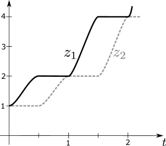
Figure 1: Iterating the exponential function $2^{x}$ with an ODE.

$$\left|b-z_{1}(1/2)\right|=\left|f(x_{0})-z_{1}(1/2)\right|\leq 1/5\text{.}$$

On the time interval $[1/2,1]$, the roles of $z_{1}$ and $z_{2}$ are switched: we will have $z_{1}^{\prime}(t)=0$ which implies that $z_{1}(t)=z_{1}(1/2)$ for all $t\in[1/2,1]$. We thus conclude that $r(z_{1}(t))=f(x_{0})$ for $t\in[1/2,1]$ and therefore the second equation of (14) behaves like the targeting equation (9) with $b=r(z_{1}(t))=f(x_{0})$, $t_{0}=1/2$, $t_{1}=1$, and $\phi(t)=\theta_{j}(-\sin 2\pi t)$ and $\tilde{c}=206$. Again, using Lemma 12 and similar arguments as in the previous case, we conclude that

$$\left|b-z_{2}(1)\right|=\left|f(x_{0})-z_{2}(1)\right|\leq 1/5\text{.}$$

In the following time interval $[1,3/2]$, the cycle repeats itself and we have $z_{2}^{\prime}(t)=0$ and thus $\tilde{f}(r(z_{2}))=f(f(x_{0}))=f^{[2]}(x_{0})$. Using a similar reasoning, we conclude that for all $k\in\mathbb{N}_{0}$ we have $z_{2}(t)=f^{[k]}(x_{0})$ for all $t\in[k,k+1/2]$, (assuming $f^{[0]}(x)=x$) and $z_{1}(t)=f^{[k+1]}(x_{0})$ for all $t\in[k+1/2,k+1]$.

We thus have shown how to iterate (the extension of) a discrete function $f:\mathbb{N}\rightarrow\mathbb{N}$ with an ODE. Nonetheless, the ODE is still not analytic as required. Remark that if the ODE is analytic, then $z_{1}^{\prime}$ and $z_{2}^{\prime}$ cannot be $0$ in half-unit intervals, since it is well-known that if an analytic function ($z_{1}^{\prime}$ and $z_{2}^{\prime}$ in our case) takes the value zero in a non-empty interval, then this function has to be identically equal to $0$ on all its domain. Therefore, instead of requiring that $z_{1}^{\prime}$ and $z_{2}^{\prime}$ take the value $0$ in alternating half-unit intervals, we require that these functions take values very close to zero. Since the map $g_{M}$ given by Theorem 9 is robust to perturbations on its input, this will ensure that the whole simulation of $g_{M}$ with a two-dimensional ODE can still be performed, even if $z_{1}$ and $z_{2}$ are not strictly constant in the half-intervals $[k+1/2,k+1]$ and $[k,k+1/2]$, respectively. However, we still have to ensure that $\left|z_{1}^{\prime}(t)\right|$ and $\left|z_{2}^{\prime}(t)\right|$ are sufficiently small in the half-unit intervals of interests to guarantee that the iteration can be carried faithfully. To better understand how this can be achieved, we have to analyze the effects of introducing perturbations in (14), with the help of Lemma 13 since now the “targets” will be slightly perturbed.

Proceeding as in [GCB08], the non-analytic function $\theta_{j}(\sin 2\pi t)$ in the first equation of (14) is replaced by an analytic periodic function with period 1 which is close to zero when $t\in[1/2,1]$. As shown in [GCB08], this can be done by considering the function $s$ defined by

$$s(t)=\frac{1}{2}\left(\sin^{2}(2\pi t)+\sin(2\pi t)\right).$$ (15)

which ranges between $0$ and $1$ in $[0,1/2]$ (and, in particular, between $4/5$ and $1$ when $x\in[0.17,0.33]$), and between $-\frac{1}{8}$ and $0$ on the time interval $[1/2,1]$. Then we take the analytic function $\phi:\mathbb{R}^{2}\rightarrow[0,1]$ defined by

$$\phi(t,y)=\Psi(s(t),y),$$

we conclude that $\int_{0}^{1/2}\phi(t,y)dt>4/5\times(0.33-0.17)=0.128>0$ (assuming that $y\geq 5)$ and $\left|\phi(t,y)\right|<e^{-y}/8$ for all $t\in[1/2,1]$ (i.e. $y$ allows us to provide an error bound for $z_{1}^{\prime}(t)$ in the time interval $[1/2,1]$). Since $\phi$ has period $1$ on $t$, we conclude that $\int_{k}^{k+1/2}\phi(t,y)dt>0.128>0$ and $\left|\phi(t,y)\right|<e^{-y}/8$ for all $t\in[k+1/2,k+1]$, where $k\in\mathbb{N}$ is arbitrary and $y\geq 5$. Therefore $\phi$ satisfies the assumptions of the function $\phi$ in Lemma 13 on the time interval $[0,1/2]$.

We can now proceed with the main construction that simulates the iteration of the map given by Theorem 9 with an analytic ODE. Take $\gamma>0$ to be a value such that $2\gamma+\delta/2\leq 1/5$, and let $g_{M}$ be the map given by Theorem 9 (use as value for $\delta$ in the statement of the Theorem 9 the value $\eta/2<1/5$, where $\eta=\left(\gamma+\delta\right)/2+1/5<2/5$). Consider the ODE $z^{\prime}=h_{M}(t,z)$ given by

$$z_{1}^{\prime} =c_{1}(z_{1}-\sigma^{[l]}\circ g_{M}\circ\sigma^{[l]}(z_{2}))^{3}\,\phi_{1}(t,z_{1},z_{2}),$$ (16)

$$z_{2}^{\prime} =c_{2}(z_{2}-\sigma^{[l]}(z_{1}))^{3}\,\phi_{2}(t,z_{1},z_{2}),$$

where $z(t)=(z_{1}(t),z_{2}(t))\in\mathbb{R}^{2}$, with initial conditions $z_{1}(0)=\bar{x}_{0}$, $z_{2}(0)=\bar{y}_{0}$, where $\bar{x}_{0},\bar{y}_{0}\in\mathbb{R}$ are approximations of some initial configuration $x_{0}$ satisfying $\left|\bar{x}_{0}-x_{0}\right|\leq 1/5$ and $\left|\bar{y}_{0}-x_{0}\right|\leq 1/5$, $l\in\mathbb{N}$ is such that $\sigma^{[l]}(\eta)\leq\gamma<1/5$ (see Lemma 5), and

$$\phi_{1}(t,z_{1},z_{2}) =\phi\left(t,\tfrac{c_{1}}{\gamma}(z_{1}-\sigma^{[l]}\circ g_{M}\circ\sigma^{[l]}(z_{2}))^{4}+\tfrac{c_{1}}{\gamma}+10\right),$$

$$\phi_{2}(t,z_{1},z_{2}) =\phi\left(-t,\tfrac{c_{2}}{\gamma}(z_{2}-\sigma^{[l]}(z_{1}))^{4}+\tfrac{c_{2}}{\gamma}+10\right),$$ (17)

and $c_{1},c_{2}$ are constants associated to a targeting error of value $\gamma$ (i.e. they are chosen such as the constant $c$ in (10) and by noting that $\int_{0}^{1/2}\phi(t,y)>0.128$, we can take $c_{1},c_{2}=4\gamma^{-2}$). Note that, since $\phi$ satisfies the assumptions of function $\phi$ in Lemma 13, the same will happen to $\phi_{1}$ and $\phi_{2}$. The ODE (16) simulates the Turing machine $M$ similarly to the ODE (14), by iterating $g_{M}$. However (17) has a more complicated expression, since it has to deal with the fact that $z_{1}^{\prime}(t)$ and $z_{2}^{\prime}(t)$ are not exactly zero in half-unit intervals.

Since we want that the ODE $z^{\prime}=h_{M}(t,z)$ to robustly simulate $M$, let us assume that the right hand-side of the equations in (16) can be subject to an error of absolute value not exceeding $\delta$. To start the analysis of the behavior of (16), let us first consider the time interval $[0,1/2]$. Since$\ \left|x\right|^{3}\leq x^{4}+1$ for all $x\in\mathbb{R}$, we conclude that $\phi_{2}$ is less than $\min(\gamma(c_{2}\left|{z}_{2}-\sigma^{[n_{2}]}({z}_{1})\right|^{3})^{-1},1/10)$. This implies, together with the assumption that $z_{2}^{\prime}$ in (17) is perturbed by an amount not exceeding $\delta$, that $\left|z_{2}^{\prime}(t)\right|\leq\gamma+\delta$ for all $t\in[0,1/2]$ which implies that $\left|z_{2}(t)-z_{2}(0)\right|\leq(\gamma+\delta)/2$ for all $t\in[0,1/2]$. Since the initial condition $\bar{x}_{0}$ satisfies $\left|\bar{x}_{0}-x_{0}\right|\leq 1/5$ where $x_{0}\in\mathbb{N}$, we conclude that

$$\left|{z}_{2}(t)-x_{0}\right|\leq\frac{\gamma+\delta}{2}+1/5=\eta<\frac{2}{5}\text{ \ \ \ for all }t\in[0,1/2]$$

which implies that

$$\left|\sigma^{[l]}(z_{2}(t))-x_{0}\right|\leq\gamma<\frac{1}{5}\text{ \ \ \ for all }t\in[0,1/2].$$

Due to Theorem 9, we conclude that

$$\left|g_{M}\circ\sigma^{[l]}(z_{2}(t))-\psi(x_{0})\right|\leq\frac{1}{5}\text{ \ \ \ for all }t\in[0,1/2].$$

Since $\sigma^{[l]}(\eta)\leq\gamma$ and $\eta>1/5$, we get that $\left|\sigma^{[l]}\circ g_{M}\circ\sigma^{[l]}(z_{2}(t))-g_{M}(x_{0})\right|<\gamma$ for all $t\in[0,1/2]$. Then the behavior of $z_{1}$ is given by Lemma 13 and

$$\left|{z}_{1}\left(\frac{1}{2}\right)-\psi(x_{0})\right|<2\gamma+\delta/2\leq\frac{1}{5}.$$ (18)

In the next half-unit interval $[1/2,1]$ the roles of ${z}_{1}$ and ${z}_{2}$ are switched as before and one concludes, using similar arguments to those used in the time interval $[0,1/2]$ that $\left|z_{1}^{\prime}(t)\right|\leq\gamma+\delta$ for $t\in[1/2,1]$. Therefore $\left|z_{1}(t)-z_{1}(1/2)\right|\leq(\gamma+\delta)/2$ for all $t\in[1/2,1]$. This inequality together with (18) yields that

$$\left|{z}_{1}(t)-\psi(x_{0})\right|<1/5+(\gamma+\delta)/2=\eta\text{ \ \ \ for all }t\in[1/2,1].$$

Since $\sigma^{[l]}(\eta)\leq\gamma$, we conclude that $\left|\sigma^{[l]}({z}_{1}(t))-\psi(x_{0})\right|\leq\gamma$ and Lemma 13 gives us

$$\left|{z}_{2}\left(1\right)-\psi(x_{0})\right|<2\gamma+\delta/2\leq\frac{1}{5}.$$ (19)

On the time interval $[1,3/2]$, the roles of $z_{1}$ and $z_{2}$ are again switched. There we will have $\left|z_{2}^{\prime}(t)\right|\leq\gamma+\delta$ for all $t\in[1,3/2]$ which implies that $\left|z_{2}(t)-z_{2}(1)\right|\leq(\gamma+\delta)/2$ for all $t\in[1/2,1]$. This inequality together with (19) gives us

$$\left|{z}_{2}(t)-\psi(x_{0})\right|<1/5+(\gamma+\delta)/2=\eta\text{ \ \ \ for all }t\in[1,3/2].$$

We thus conclude that this analysis can be repeated in subsequent time intervals and thus that for all $j\in\mathbb{N}$, if $t\in[j,j+\frac{1}{2}]$ then $\left|z_{2}(t)-\psi^{[j]}(x_{0})\right|\leq 1/5$. This concludes the proof.

Remark 15

From the proof of Theorem 11, we conclude that if the Turing machine halts after $n_{0}$ steps with configuration $c_{h}$ and if we assume that $\psi(c_{h})=c_{h}$, then for any $n\in\mathbb{N}$ satisfying $n\geq n_{0}+1$, we have

$$\left|{z}_{2}\left(n\right)-c_{h}\right|\leq\frac{1}{5}.$$

Furthermore, on the half-unit time interval $[n,n+1/2]$, we will get that

$$\left|\sigma^{[l]}({z}_{1}(t))-c_{h}\right|<\gamma<1/5$$

for $t\in[n,n+1/2]$. Assuming that $\delta=0$ in Theorem 11, we then conclude from (16) that $z_{2}(t)$ starts its trajectory from a value $1/5$-near to $c_{h}$ and will monotically converge to a value $\sigma^{[l]}({z}_{1}(t))$ which, although may change with time, will never leave an $1/5$-vicinity of $c_{h}$ for $t\in[n,n+1/2]$. This implies that

$$\left|{z}_{2}\left(t\right)-c_{h}\right|\leq\frac{1}{5}$$ (20)

for all $t\in[n,n+1/2]$. Since (20) holds on $[n,n+1/2]$ as we have seen from the proof of Theorem 11, we conclude that (20) holds for $t\geq n_{0}+1/2$.

6 Simulating Turing machines over compact sets

So far all our simulations of Turing machines are carried out over the non-compact set $\mathbb{R}^{n}$. In this section we show that it is possible to simulate Turing machines with ODEs on the 2-dimensional compact sphere $\mathbb{S}^{2}=\{x\in\mathbb{R}^{3}:\left\|x\right\|=1\}$. The technique used in the construction is based on a similar result proved in [CMPS21]. It is shown in [CMPS21] that there is a computable polynomial vector field on the sphere $\mathbb{S}^{n}=\{x\in\mathbb{R}^{n+1}:\left\|x\right\|=1\}$ simulating a universal Turing machine; in other words, the polynomial vector field is Turing complete, where $n\geq 17$ is arbitrary. The underlying idea of the construction presented in [CMPS21] is to map a vector field defined in $\mathbb{R}^{n}$ to $\mathbb{S}^{n}$ using the stereographic projection, and to remove the singularity at the north pole by using a suitable reparametrization on the polynomial vector fields. We show in this section that the dimension can be lowered from $n\geq 17$ to $n=2$ at the cost of using a non-polynomial $C^{\infty}$ vector field.

The notion introduced in the following definition will be used throughout this section.

Definition 16

Let $f:\mathbb{R}^{n+k}\rightarrow\mathbb{R}^{j}$, where $n,k,j\in\mathbb{N}_{0}$, with $j\geq 1$. Given an expression $f(x_{1},\ldots,x_{n},y_{1},\ldots,y_{k})$, we say that $f$ is bounded by a constant on the variables $x_{1},\ldots,x_{n}$ and bounded by a polynomial on the variables $y_{1},\ldots,y_{k}$ if

$$\left\|f(x_{1},\ldots,x_{n},y_{1},\ldots,y_{k})\right\|\leq p(y_{1},\ldots,y_{k})$$

for all $(x_{1},\ldots,x_{n},y_{1},\ldots,y_{k})\in\mathbb{R}^{n+k}$ in the domain of $f$.

For example $g(t,x)=x\sin(2\pi t)$ is bounded by a constant on $t$ and polynomially bounded on $x$ and $h(t)=\sin(2\pi t)$ is bounded by a constant on $t$ (to simplify notation, in this latter case where $h$ is not polynomially bounded on any other variables, we will just say that $h$ is bounded by a constant). Some functions which are bounded by a constant include $\sin$, $\cos$, $\arctan$.

The next result shows when a Turing universal vector field can be defined on $\mathbb{S}^{n}$.

Theorem 17

Let

$$y^{\prime}=f(t,y)$$ (21)

be a $C^{1}$-computable ODE simulating a Turing machine $M$, where $f:\mathbb{R}^{n+1}\rightarrow\mathbb{R}^{n}$ is a $C^{\infty}$ function with the property that both $f$ and all its partial derivatives $\frac{\partial^{\left|k\right|}f}{\partial t^{k_{0}}\partial y_{1}^{k_{1}}\ldots\partial y_{n}^{k_{n}}}$ are bounded by a constant on $t$ and are polynomially bounded on the variables $x_{1},\ldots,x_{n}$, assuming that the argument of $f$ is $(t,x)\in\mathbb{R}^{n+1}$, where $k_{0},k_{1},\ldots,k_{n}\in\mathbb{N}_{0}$, $k=(k_{0},k_{1},\ldots,k_{n})$, and $\left|k\right|=k_{0}+k_{1}+\ldots+k_{n}$. Then from $f$ one can compute a $C^{\infty}$ vector field $F$ defined on $\mathbb{S}^{n}$ that also simulates $M$.

Proof. We recall that the (inverse) stereographic projection $\varphi:\mathbb{R}^{n}\rightarrow\mathbb{S}^{n}\subseteq\mathbb{R}^{n+1}$ is given by

$$\varphi(x_{1},x_{2},\ldots,x_{n})=\left(\frac{r^{2}-1}{1+r^{2}},\frac{2x_{1}}{1+r^{2}},\frac{2x_{2}}{1+r^{2}},\ldots,\frac{2x_{n}}{1+r^{2}}\right)$$

where $r^{2}=x_{1}^{2}+x_{2}^{2}+\ldots+x_{n}^{2}$. Suppose that $f(t,x)=(f_{1}(t,x),\ldots,f_{n}(t,x))$. Then we can write the vector field defined by $f$ on $\mathbb{R}^{n}$ as

$$f=\sum_{i=1}^{n}f_{i}\frac{\partial}{\partial x_{i}}.$$

We recall that if $g:M\rightarrow N$ is a $C^{1}$ map between two manifolds $M=\mathbb{R}^{n}$ and $N=\mathbb{R}^{k}$, then for each $p\in M$ the map $g$ induces a linear map $g_{\ast}:T_{p}M\rightarrow T_{g(p)}N$ from the tangent space $T_{p}M$ of $M$ at $p$ to the tangent space of $N$ at $g(p)$. We also recall that $(\left.\partial/\partial x_{1}\right|_{p},\ldots,\left.\partial/\partial x_{n}\right|_{p})$ forms a basis for $T_{p}M\$and, similarly, if $(\bar{x}_{1},\ldots,\bar{x}_{k})$ are coordinates for $N=\mathbb{R}^{k}$, then $(\left.\partial/\partial\bar{x}_{1}\right|_{g(p)},\ldots,\left.\partial/\partial\bar{x}_{k}\right|_{g(p)})$ forms a basis for $T_{g(p)}N$. Moreover, the matrix that (locally) defines the linear map $g_{\ast}$, relative to the bases $(\left.\partial/\partial x_{1}\right|_{p},\ldots,\left.\partial/\partial x_{n}\right|_{p})$ and $(\left.\partial/\partial\bar{x}_{1}\right|_{g(p)},\ldots,\left.\partial/\partial\bar{x}_{k}\right|_{g(p)})$, is the Jacobian of $g$. In the case of the map $\varphi$, and if we take $(y_{0},y_{1},\ldots,y_{n})$ as coordinates for $\mathbb{R}^{n+1}$, we obtain the following (note that the variable $t$ in the expression of $f$ can be seen as a fixed parameter):

$$\varphi_{\ast}\left(f\right) =\sum_{i=1}^{n}f_{i}\varphi_{\ast}\left(\frac{\partial}{\partial x_{i}}\right)$$

$$=\sum_{i=1}^{n}f_{i}\sum_{j=0}^{n}\frac{\partial\varphi_{j}}{\partial x_{i}}\frac{\partial}{\partial y_{j}}$$

$$=\sum_{i=1}^{n}f_{i}\cdot\left((1-y_{0})y_{i}\frac{\partial}{\partial y_{0}}+(1-y_{0}-y_{i}^{2})\frac{\partial}{\partial y_{i}}-\sum_{\begin{subarray}{c}j=0\\ j\notin\{0,i\}\end{subarray}}^{n}y_{i}y_{j}\frac{\partial}{\partial y_{j}}\right),$$ (22)

where $f_{i}$ is evaluated at $(t,\varphi^{-1}(y_{0},y_{1},\ldots,y_{n}))=\left(t,\frac{y_{1}}{1-y_{0}},\ldots,\frac{y_{n}}{1-y_{0}}\right)$. This implies that $\varphi_{\ast}\left(f\right)$ is a vector field of class $C^{\infty}$, except at the north pole $y_{NP}=(1,0,\ldots,0)$ of $\mathbb{S}^{n}$ where it is not defined. Let us now consider the following ODE

$$\tau^{\prime} =K(\bar{x})$$ (23)

$$\bar{x}^{\prime} =f(\tau,\bar{x})K(\bar{x})$$

where $K:\mathbb{R}^{n}\rightarrow\mathbb{R}$ is such that $K(x)>0$ for any $x\in\mathbb{R}^{n}$ and $\tau(0)=0$, $\bar{x}(0)=x_{0}$. Since $\tau^{\prime}(t)>0$, $\tau$ is strictly increasing and thus $\tau$ admits an inverse $\tau^{-1}$. Next we note that if $\tilde{x}=x\circ\tau$, where $x$ is a solution of (21) and $\tau(0)=0$, we have that

$$\tilde{x}^{\prime}(t) =\left(x(\tau(t))\right)^{\prime}$$

$$=f(\tau(t),x(\tau(t)))\tau^{\prime}(t)$$

$$=f(\tau(t),\tilde{x}(t))K(\bar{x}(t)).$$ (24)

It is not difficult to see that if $(\tau,\bar{x})$ is a solution for (23), then $\bar{x}$ is also a solution to (24). Since the solution of the ODE (23) is unique, by the Picard-Lindelöf theorem, we conclude that $\bar{x}(t)=\tilde{x}(t)=x(\tau(t))$. Furthermore, since $\tau^{\prime}(t)>0$ for any $t\in\mathbb{R}$, we conclude that any solution curve of (21) with initial condition $y(0)=x_{0}$ also provides a solution curve for the last $n$ components of the solution of (23) with initial condition $\tau(0)=0$, $\bar{x}(0)=x_{0}$, up to some time reparametrization, and vice versa.

Thus, by taking $K(x)=e^{-\frac{2}{1+r^{2}}}=e^{-\frac{2}{1+x_{1}^{2}+\ldots+x_{n}^{2}}}$, we conclude that the solution curves of

$$\tau^{\prime} =e^{-\frac{2}{1+r^{2}}}$$

$$x^{\prime} =e^{-\frac{2}{1+r^{2}}}f(\tau,x)=h(t,x)$$ (25)

and of (21) are the same, up to a time reparametrization $\tau$ given by the ODE $\tau^{\prime}=e^{-\frac{2}{1+r^{2}}}>0$. Note that the right-hand side of (25) is formed by $C^{1}$-computable functions, which means that the solution $(\tau,x)$ to (25) is also computable, since the solution to a $C^{1}$-computable system is also computable [GZB09], [CG08]. Hence, when simulating Turing machines, if the result of the $n$th step of the computation of the Turing machine being simulated by (21) can be read in the time interval $[a_{n},b_{n}]$, then the result of the $n$th step when the simulation is performed by (25) can be read on the time interval $[\tau^{-1}(a_{n}),\tau^{-1}(b_{n})]$. Note that $\tau^{-1}$ can be computed from $\tau$ and hence from $f$. Indeed, we know that the derivative of $\tau^{-1}$ is given by

$$\left(\tau^{-1}(a)\right)^{\prime} =\frac{1}{\tau^{\prime}(\tau^{-1}(a))}$$

$$=\frac{1}{K(\bar{x}(\tau^{-1}(a)))}$$

$$=\frac{1}{K(x(\tau\circ\tau^{-1}(a)))}$$

$$\frac{1}{K(x(a))}.$$

Hence $\tau^{-1}$ can be obtained as the solution of the initial-value problem (IVP) defined by $\left(\tau^{-1}(t)\right)^{\prime}=1/K(x(t))$, $\tau^{-1}(0)=0$. Since the right-hand side of the ODE defining this IVP is computable from $x$ and hence from $f$, we conclude that $\tau^{-1}$ is computable from $f$ [GZB09], [CG08]. In particular, if $f$ is computable, then so is $\tau^{-1}$.

We now have (we can again assume that $t$ is a fixed parameter for $h$, where $h$ is given by (25))

$$\varphi_{\ast}\left(h\right)=e^{-(1-y_{0})}\varphi_{\ast}\left(f\right).$$

From (22) we conclude that (note that $\left|y_{i}\right|\leq 1$)

$$\left\|\varphi_{\ast}\left(h\right)(y)\right\| =\left\|e^{-(1-y_{0})}\varphi_{\ast}\left(f\right)(y)\right\|$$

$$=\left\|e^{-(1-y_{0})}\right\|\left\|\varphi_{\ast}\left(f\right)(y)\right\|$$

$$=\left\|e^{-(1-y_{0})}\right\|\left\|\sum_{i=1}^{n}f_{i}\left(t,\frac{y_{1}}{1-y_{0}},\ldots,\frac{y_{n}}{1-y_{0}}\right)\right.\cdot$$

$$\cdot\left.\left((1-y_{0})y_{i}\frac{\partial}{\partial y_{0}}+(1-y_{0}-y_{i}^{2})\frac{\partial}{\partial y_{i}}-\sum_{\begin{subarray}{c}j=0\\ j\notin\{0,i\}\end{subarray}}^{n}y_{i}y_{j}\frac{\partial}{\partial y_{j}}\right)\right\|$$

$$\leq e^{-(1-y_{0})}\cdot 6n\cdot p\left(\frac{y_{1}}{1-y_{0}},\ldots,\frac{y_{n}}{1-y_{0}}\right).$$

This latter result implies that

$$\lim_{\begin{subarray}{c}y\rightarrow y_{NP}\\ y\in\mathbb{S}^{n}-\{y_{NP}\}\end{subarray}}\varphi_{\ast}\left(h\right)(y)=0.$$ (26)

Similarly, if we assume that

$$\varphi_{\ast}\left(h\right)(y)=e^{-(1-y_{0})}\sum_{i=0}^{n}s_{i}(t,y)\frac{\partial}{\partial y_{i}}$$

where $s_{i}$ are functions, from (22) and from the assumption that all the partial derivatives of $f$ of the form $\frac{\partial^{|k|}f}{\partial t^{k_{0}}\partial x_{1}^{k_{1}}\ldots\partial x_{n}^{k_{n}}}$ are polynomially bounded on $x_{1},\ldots,x_{n}$, we can conclude that each partial derivative of $s_{i}$ is polynomially bounded by some polynomial $\tilde{p}\left(\frac{y_{1}}{1-y_{0}},\ldots,\frac{y_{n}}{1-y_{0}}\right)$, which implies that

$$\lim_{\begin{subarray}{c}y\rightarrow y_{NP}\\ y\in\mathbb{S}^{n}-\{y_{NP}\}\end{subarray}}\frac{\partial^{|k|}\varphi_{\ast}\left(h\right)(y)}{\partial t^{k_{0}}\partial y_{1}^{k_{1}}\ldots\partial y_{n}^{k_{n}}}=0.$$

Therefore we can extend $\varphi_{\ast}\left(h\right)(y)$ to a $C^{\infty}$ vector field $\tilde{g}$ defined on the entire sphere $\mathbb{S}^{n}$ if we assume that the value of $\tilde{g}$ and of its partial derivatives is $0$ at the north pole $y_{NP}=(1,0,\ldots,0)$ of $\mathbb{S}^{n}.$ We thus have defined a $C^{\infty}$ vector field $\tilde{g}$ on the entire sphere $\mathbb{S}^{n}$, and $\tilde{g}$ is Turing universal.   

With the help of the above theorem, we may hope we could just make use of the vector field $g_{M}$ of Theorem 11 as the vector field $f$ in Theorem 17 to prove that there is a Turing universal vector field in $\mathbb{S}^{2}$. However, there are several problems with this approach as listed below: (1) the approach requires that $g_{M}(t,x_{1},x_{2})$ and all of its partial derivatives are bounded by a constant on $t$ and are polynomially bounded on $x_{1}$ and $x_{2}$. A major problem in this respect is that $g_{M}$ uses in its expression the function $\Psi$ defined in Lemma 4 that does not necessarily have polynomially bounded derivatives because the function $\arcsin$ is used in the definition of $\Psi$ and the derivative of $\arcsin$ is not polynomially bounded as its argument approaches $-1$ or $1$. (2) The expression of $g_{M}$ relies on the expression of the function $\bar{g}_{M}$ given by Theorem 3. Thus one must show that $\bar{g}_{M}(t,x_{1},x_{2},x_{3},y_{1},y_{2},y_{3})$ is bounded polynomially on $x_{1},x_{2},x_{3},y_{1},y_{2},y_{3}$. (3) The argument of the functions $\Omega_{k,i}:\mathbb{R\rightarrow R}$ from Proposition 8 is provided as the initial condition of an ODE. It is not straightforward to analyze the dependence of $\Omega_{k,i}$ and of its derivatives on its argument.

In the following we present the solutions to the listed problems. First we note that in Theorem 17 the vector field is no longer required to be analytic (it only has to be $C^{\infty}$). Therefore we can substitute the function $\Psi$ defined in Lemma 4 by the function $r:\mathbb{R\rightarrow R}$ defined in Lemma 14. We recall that the function $r$ has the property that $r(x)=n$, whenever $x\in[n-1/4,n+1/4]$, for all integers $n$. Thus if we take $\Psi(x,y)=r(x)$, the properties stated for $\Psi$ in Lemma 4 remain true. Therefore, we can replace $\Psi$ with $r$ when defining the vector field $g_{M}$ of Theorem 11. In this case, the properties stated in Theorem 11 remain true with $g_{M}$ being a $C^{\infty}$ function rather than an analytic function. However, we gain the advantage that $r$ and its derivatives are polynomially bounded as we shall show now. Indeed, it follows from its definition that $\left|r(x)\right|\leq\left|x\right|+1\leq x^{2}+2$ (recall that $\left|x\right|\leq x^{2}+1$). For the derivatives of $\theta$, we note that if $a(x)=e^{-1/x}$, then it is readily seen by induction that for each $n\in\mathbb{N}_{0}$ there is a polynomial $P_{n}$ such that $a^{(n)}(x)=P_{n}(1/x)e^{-1/x}$, with $a^{(0)}(x)=a(x)$ (and thus $P_{0}=1$). This implies that $\lim_{x\rightarrow 0^{+}}a^{(n)}(x)=0$ and $\lim_{x\rightarrow+\infty}a^{(n)}(x)=K_{n}$, where $K_{n}$ is the constant term of $P_{n}$. Therefore, by definition of the limit, there exists $b_{n},\varepsilon_{n}>0$ such that $\left|a^{(n)}(x)\right|\leq 1$ whenever $x\in(0,\varepsilon_{n}]$ and $\left|a^{(n)}(x)\right|\leq K_{n}+1$ whenever $x\geq b_{n}$. Now set $M_{n}=\max_{x\in[\varepsilon,M]}\left|a^{(n)}(x)\right|\mathbb{\in R}$. Then $\left|a^{(n)}(x)\right|\leq\max(1,K_{n}+1,M_{n})$ for all $x\in(0,+\infty)$, which implies that $\theta$ in (12) as well as its derivatives are polynomially bounded on $[0,+\infty)$. Consequently, the function $v$ from (13) as well as the derivatives of $v$ are polynomially bounded following Lemmas 18 and 19 to be presented in a moment. Lemma 14 together with Lemmas 18 and 19 then imply that $r$ as well as its derivatives are polynomially bounded.

Some notations are in order for the statements of the next two lemmas. Given multi-indexes $\alpha=(\alpha_{1},\ldots,\alpha_{n}),\beta=(\beta_{1},\ldots,\beta_{n})\in\mathbb{N}_{0}^{n}$ and $x=(x_{1},\ldots,x_{n})\in\mathbb{R}^{n}$, let

$$\left|\alpha\right| =\alpha_{1}+\ldots+\alpha_{n}$$

$$\alpha+\beta =(\alpha_{1}+\beta_{1},\ldots,\alpha_{n}+\beta_{n})$$

$$\alpha! =(\alpha_{1}!)\cdot(\alpha_{2}!)\cdot\ldots\cdot(\alpha_{n}!)$$

$$\beta \leq\alpha\text{ iff }\beta_{1}\leq\alpha_{1},\ldots,\beta_{n}\leq\alpha_{n}$$

$$\binom{\alpha}{\beta} =\binom{\alpha_{1}}{\beta_{1}}\ldots\binom{\alpha_{n}}{\beta_{n}}=\frac{\alpha!}{\beta!(\alpha-\beta)!}\text{ for }\beta\leq\alpha$$

$$D_{x}^{\alpha} =\frac{\partial^{\left|\alpha\right|}}{\partial x_{1}^{\alpha_{1}}\ldots\partial x_{n}^{\alpha_{n}}}\text{ \ \ (}D_{x}^{0}\text{ is the identity operator)}$$

$$x^{\alpha} =x_{1}^{\alpha_{1}}\ldots x_{n}^{\alpha_{n}}$$

Lemma 18

Suppose that $f,g:\mathbb{R}^{n}\rightarrow\mathbb{R}$ are $C^{\infty}$ functions which are bounded by a constant on the variables $x_{1},\ldots,x_{i}$ and are bounded by a polynomial on the variables $x_{i+1},\ldots,x_{n}$, as well as all their partial derivatives. Then:

1. The $C^{\infty}$ function $f\pm g:\mathbb{R}^{n}\rightarrow\mathbb{R}$ defined by $(f+g)(x)=f(x)+g(x)$ is bounded by a constant on the variables $x_{1},\ldots,x_{i}$ and bounded by a polynomial on the variables $x_{i+1},\ldots,x_{n}$, as well as all its partial derivatives.

2. The $C^{\infty}$ function $f\times g:\mathbb{R}^{n}\rightarrow\mathbb{R}$ defined by $(f\times g)(x)=f(x)\cdot g(x)$ is bounded by a constant on the variables $x_{1},\ldots,x_{i}$ and bounded by a polynomial on the variables $x_{i+1},\ldots,x_{n}$, as well as all its partial derivatives.

Proof. Let $\alpha=(\alpha_{1},\ldots,\alpha_{n})$ be a multi-index. For point 1, we note that

$$\frac{\partial^{\left|\alpha\right|}}{\partial x^{\alpha}}(f\pm g)(x)=\frac{\partial^{\left|\alpha\right|}f(x)}{\partial x^{\alpha}}\pm\frac{\partial^{\left|\alpha\right|}g(x)}{\partial x^{\alpha}}$$

and thus the result follows immediately from the assumption.

For the product $f\times g$, the claim follows directly from the general Leibniz rule for multivariate functions (see e.g. [CS96, Proof of Lemma 2.6]):

$$\frac{\partial^{\left|\alpha\right|}}{\partial x^{\alpha}}(f\times g)(x)=\sum_{0\leq\beta\leq\alpha}\binom{\alpha}{\beta}\frac{\partial^{\left|\beta\right|}f(x)}{\partial x^{\beta}}\frac{\partial^{\left|\alpha-\beta\right|}g(x)}{\partial x^{\alpha-\beta}}.$$

 

Lemma 19

Suppose that $f:\mathbb{R}^{j}\rightarrow\mathbb{R}^{n}$ and $g:\mathbb{R}^{k}\rightarrow\mathbb{R}^{j}$ are $C^{\infty}$ functions with the following properties:

1. $f$ and its partial derivatives are polynomially bounded on its arguments $z_{1},\ldots,z_{j}$;

2. $g$ and its partial derivatives are bounded by a constant on the variables $x_{1},\ldots,x_{i}$ and bounded by a polynomial on the variables $x_{i+1},\ldots,x_{k}$.

Then $f\circ g$ is a $C^{\infty}$ function with the property that $f\circ g$ as well as all its partial derivatives are bounded by a constant on the variables $x_{1},\ldots,x_{i}$ and by a polynomial on the variables $x_{i+1},\ldots,x_{k}$.

Proof. To prove this theorem, we will use a multivariate version of the Faà di Bruno formula which allows us to compute the higher order partial derivatives of the composition of multivariate functions $f$ and $g$. Some notational matter is in order first. Let $\alpha=(\alpha_{1},\ldots,\alpha_{n})\in\mathbb{N}_{0}^{n}$ be a multi-index. Then following the approach of [Ma09], let us assume that $\chi^{0}=1$ regardless of whether $\chi$ is a number or a differential operator. We say that a multi-index $\alpha$ can be decomposed into $s$ parts $p_{1},\ldots,p_{s}\in\mathbb{N}_{0}^{n}$ with multiplicities $m_{1},\ldots,m_{s}\in\mathbb{N}_{0}^{d}$ if the decomposition $\alpha=\left|m_{1}\right|p_{1}+\ldots+\left|m_{s}\right|p_{s}$ holds and all parts are different. In this case the total multiplicity is defined as $m=m_{1}+\ldots+m_{s}$. The list $(s,p,m)$ is called a $d$-decomposition, or simply just a decomposition, of $\alpha$. Then, assuming that $z=f\circ g(x)$ and $y=g(x)$, we have

$$\frac{\partial^{\left|\alpha\right|}}{\partial x^{\alpha}}f\circ g(x)=\alpha!\sum_{(s,p,m)\in\mathcal{D}}\frac{\partial^{\left|m\right|}}{\partial y^{m}}f(g(x))\prod_{k=1}^{s}\frac{1}{m_{k}!}\left(\frac{1}{p_{k}!}\frac{\partial^{\left|p_{k}\right|}}{\partial x^{p_{k}}}g(x)\right)f\circ g(x)$$

where $\mathcal{D}$ is the set of all decompositions of $\alpha$. From this later formula and the the hypothesis on $f$, $g$ we conclude that $f\circ g$ is a $C^{\infty}$ function with the property that $f\circ g$ as well as all its partial derivatives are bounded by a constant on the variables $x_{1},\ldots,x_{i}$ and are bounded by a polynomial on the variables $x_{i+1},\ldots,x_{k}$.   

Since the function $f_{M}$ of Theorem 1 can be written using only the following terms: variables, polynomial-time computable constants, $+$, $-$, $\times$, $\sin$, $\cos$, $\arctan$, we conclude from Lemmas 18 and 19 that $f_{M}$ as well as all its partial derivatives are bounded by a polynomial. Furthermore, as the function $g_{M}$ from Theorem 9 is obtained using the functions $\Upsilon_{3},f_{M},\Omega_{3,1},\Omega_{3,2},\Omega_{3,3},\sigma$, again by Lemmas 18 and 19 it suffices to show that $\Upsilon_{3},\Omega_{3,1},\Omega_{3,2},\Omega_{3,3},\sigma$ as well as their partial derivatives are (or can be made) bounded by a polynomial. The case of the function $\sigma$ in Lemma 5 is immediate from Lemmas 18 and 19. The case of $\Upsilon_{3}$ can be treated by replacing $\Psi(x,y)$ in the expression of $\Upsilon_{3}$ given in the proof of Proposition 7 by the $C^{\infty}$ function $r$, as explained above. Then it follows immediately that $\Upsilon_{3}$ maintains its properties given by Proposition 7, except analiticity ($\Upsilon_{3}$ will only be $C^{\infty}$) and, meanwhile, Lemmas 18 and 19 imply that $\Upsilon_{3}$ and its partial derivatives are polynomially bounded.

The situation for $\Omega_{3,1},\Omega_{3,2},\Omega_{3,3}$ is more subtle, as the arguments to these functions are passed as initial conditions of an ODE. What we are going to do is to create new $C^{\infty}$ functions $\overline{\Omega}_{3,1},\overline{\Omega}_{3,2},\overline{\Omega}_{3,3}$ such that these new functions maintain the useful properties of $\Omega_{3,1},\Omega_{3,2},\Omega_{3,3}$ on the one hand and, on the other hand, the new functions together with their partial derivatives are polynomially bounded. Once this is done, the old functions $\Omega_{3,1},\Omega_{3,2},\Omega_{3,3}$ can then be replaced by the new functions $\overline{\Omega}_{3,1},\overline{\Omega}_{3,2},\overline{\Omega}_{3,3}$ in the expression of $g_{M}$ in the proof of Theorem 9. The function $g_{M}$ as well as its partial derivatives are now polynomially bounded on all variables except the time $t$. But since the time variable only appears inside the functions $\phi_{1}$ and $\phi_{2}$ defined by (17) in the format of $\sin(2\pi t)$ as defined in (15), and $\sin(2\pi t)$ and its derivatives are obviously bounded by a constant, it follows that the theorem below holds true.

Theorem 20

Let $\psi:\mathbb{N}\rightarrow\mathbb{N}$ be the transition function of a Turing machine $M$, under the encoding described in Section 4. Then there exist $0<\eta<2/5$ and a $C^{\infty}$ function $g_{M}:\mathbb{R}^{3}\rightarrow\mathbb{R}^{2}$ such that the ODE $z^{\prime}=g_{M}(t,z)$ simulates $M$ in the following sense: for all $x_{0}\in\mathbb{N}$ which encodes a configuration according to the encoding described above, if $\bar{x}_{0},\bar{y}_{0}\in\mathbb{R}$ satisfy the conditions $\left\|\bar{x}_{0}-x_{0}\right\|\leq 1/5$ and $\left\|\bar{y}_{0}-x_{0}\right\|\leq 1/5$, then the solution $z(t)$ of

$$z^{\prime}=g_{M}(t,z),\qquad z(0)=(\bar{x}_{0},\bar{y}_{0})$$

satisfies, for all $j\in\mathbb{N}_{0}$ and for all $t\in[j,j+1/2]$,

$$\left\|z_{2}(t)-\psi^{[j]}(x_{0})\right\|\leq\eta,$$

where $z(t)\equiv(z_{1}(t),z_{2}(t))\in\mathbb{R}^{2}$. Furthermore $g_{M}(t,z_{1},z_{2})$ and its partial derivatives are polynomially bounded on $z_{1}$ and $z_{2}$ and bounded by a constant on $t$.

Theorem 21

Let $M$ be a Turing machine. Then one can compute from $f$ a $C^{\infty}$ vector field $F$ defined on $\mathbb{S}^{2}$ which also simulates $M$.

Proof. Immediate from Theorems 17 and 20.   

It remains to show that the new $C^{\infty}$ functions $\overline{\Omega}_{3,1},\overline{\Omega}_{3,2},\overline{\Omega}_{3,3}$ can be constructed such that they retain the useful properties of $\Omega_{3,1},\Omega_{3,2},\Omega_{3,3}$, but these new functions and their partial derivatives are polynomially bounded. We begin with a preliminary lemma.

Lemma 22

Let $f:\mathbb{R}^{n+1}\rightarrow\mathbb{R}^{n}$ be a $C^{\infty}$ function such that $f$ and its partial derivatives are polynomially bounded. Suppose that $x_{f}:\mathbb{R\rightarrow R}$ is the first coordinate of a solution $x$ of the IVP

$$x^{\prime}=f(t,x).$$

If $x$ is polynomially bounded, then all the derivatives of $x_{f}$ are polynomially bounded.

Proof. We show the result by induction on the order of the derivative by showing that $x^{(k)}=f^{k}(t,x(t))$, where $f^{k}$ is a $C^{\infty}$ function which is polynomially bounded, as well as all its partial derivatives. Then we will conclude that $x^{(k)}$ is polynomially bounded as well as all its partial derivatives by Lemma 19. The base case

$$x^{\prime}(t)=f(t,x(t))$$

is trivial. Let us now assume that $x^{(k)}=f^{k}(t,x(t))$, where $f^{k}$ is polynomially bounded as well as all its partial derivatives. Then

$$x_{i}^{(k+1)}(t) =\left(f_{i}^{k}(t,x(t))\right)^{\prime}$$

$$=\frac{\partial f_{i}^{k}}{\partial t}(t,x(t))+\sum_{j=1}^{n}\frac{\partial f_{i}^{k}}{\partial y_{j}}(t,x(t))\frac{dx_{j}}{dt}(t)$$

$$=\frac{\partial f_{i}^{k}}{\partial t}(t,x(t))+\sum_{j=1}^{n}\frac{\partial f_{i}^{k}}{\partial y_{j}}(t,x(t))f_{j}^{k}(t,x(t))$$

$$=f_{i}^{k+1}(t,x(t)).$$

By taking $f^{k+1}=(f_{1}^{k+1},\ldots,f_{n}^{k+1})$, we conclude that $x^{(k+1)}=f^{k+1}(t,x(t))$ and by Lemmas 18 and 19 we conclude that $f^{k+1}$ is polynomially bounded as well as all its partial derivatives, thus showing the result.   

To define new $C^{\infty}$ functions $\overline{\Omega}_{3,1},\overline{\Omega}_{3,2},\overline{\Omega}_{3,3}$ as in Proposition 8, we recall that the key point of the proof of Proposition 8 was to consider the bijection $I:\mathbb{N}^{2}\rightarrow\mathbb{N}$ given by (4 ) and to obtain real extensions of the components $J_{2,1}$ and $J_{2,2}$ which form the inverse function of $I$, i.e. $I^{-1}(z)=(J_{2,1}(z),J_{2,2}(z))$. Then the result would follow inductively when obtaining extensions $\Omega_{k,i}$ from $J_{k,i}$ for $k>2$. Subsequently, the only required modification is to obtain suitable real extensions $\overline{\Omega}_{2,1},\overline{\Omega}_{2,2}$ of $J_{2,1},J_{2,2}$, respectively. We shall demand that if $n\in\mathbb{N}_{0}$, then $\left|\overline{\Omega}_{2,i}(z)-J_{2,i}(n)\right|\leq 1/5$ whenever $\left|z-n\right|\leq 1/4$ for $i=1,2$, so that $\overline{\Omega}_{2,i}$ has the same properties as of $\Omega_{2,i}$ regarding Proposition 8, except that $\overline{\Omega}_{2,i}$ is $C^{\infty}$ instead of analytic. We also require that $\overline{\Omega}_{2,i}$ and its derivatives are polynomially bounded. To obtain $\overline{\Omega}_{2,i}$, we first construct a $C^{\infty}$ function $\tilde{\Omega}_{2,i}$ with the property that $\left|\tilde{\Omega}_{2,i}(z)-J_{2,i}(n)\right|\leq 1/4$ whenever $z\in[n,n+1/2]$ for $i=1,2$, and $\tilde{\Omega}_{2,i}$ as well as its partial derivatives are polynomially bounded. By setting $\overline{\Omega}_{2,i}(z)=\sigma\circ\tilde{\Omega}_{2,i}(z+1/4)$, where $\sigma$ is given by Lemma 5, we conclude from the above and from Lemmas 18 and 19 that $\overline{\Omega}_{2,i}$ has the desired properties. Before defining $\tilde{\Omega}_{2,1}$ and $\tilde{\Omega}_{2,2}$, we note that $I$ is obtained by dovetailing by enumerating the pairs in the diagonals below from the (one element) diagonal starting on $(0,0)$ and then moving to the next diagonal

In other words, we have $I(0,0)=0,$ $I(0,1)=1$, $I(1,0)=2$, $I(0,2)=3$, and so on. We note that the sum of the coordinates in each diagonal is constant. From here we see that the graphs for $J_{2,1}$ and $J_{2,2}$, provided in Figures 2 and 3, respectively, have certain regularities which will be explored to obtain $\tilde{\Omega}_{2,1}$ and $\tilde{\Omega}_{2,2}$.

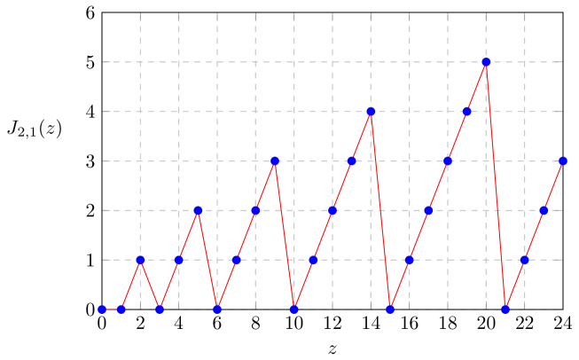
Figure 2: Graph of the function $J_{2,1}$. Since the function is discrete, the image are only the blue points (the red line is given as a visualization helper).

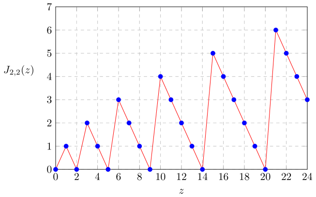
Figure 3: Graph of the function $J_{2,2}$. Since the function is discrete, the image are only the blue points (the red line is given as a visualization helper).

Let us start with the case of $\tilde{\Omega}_{2,1}$. We first analyze the behavior of $J_{2,1}$. Let us suppose that the argument $z$ of $J_{2,1}(z)$ codes a pair $(0,n)$ at the start of the diagonal with sum $n$. Then $J_{2,1}(z)=0$, $J_{2,1}(z+1)=1,$ …, $J_{2,1}(z+n)=n$, $J_{2,1}(z+n+1)=0$, $J_{2,1}(z+n+2)=1,$ … Thus to simulate $J_{2,1}$ we need to track the sum $s$ of the diagonal, and increase it by one when $J_{2,1}(z)$ reaches the value of $s$. On the next value $z+1$, we will have that $J_{2,1}(z+1)$ will take the value $0$, and each time its argument $z$ increases by one, $J_{2,1}(z)$ also increases by one, until it reaches the (new) value of the sum of the diagonal and the cycle repeats itself. We will simulate this behavior with ODEs. Before showing how this can be done, consider the auxiliary function $\xi:\mathbb{R\rightarrow R}$ defined as

$$\xi^{\prime}(x)=\left\{\begin{array}[c]{ll}0&\text{if }x\leq 1/4\\ c_{\xi}\theta(-(x-1/4)(x-3/4))\text{ \ \ }&\text{if }1/4<x<3/4\\ 0&\text{if }x\geq 3/4\end{array}\right.$$

where $\xi(x)=0$ and $c_{\xi}=\left(\int_{1/4}^{3/4}\theta(-(x-1/4)(x-3/4))dx\right)^{-1}$. It is not difficult to see that $\theta(-(x-1/4)(x-3/4))>0$ when $1/4<x<3/4$. Hence we have that $\xi(x)=0$ whenever $x\leq 1/4$, $0<\xi(x)<1$ when $1/4<x<3/4$ and $\xi(x)=1$ when $x\geq 3/4$. Furthermore $\xi$ is $C^{\infty}$ and $\xi$ and all its derivatives are polynomially bounded due to Lemmas 18 and 19.

Let us now present the ODE which will define $\tilde{\Omega}_{2,1}$

$$\left\{\begin{array}[c]{l}x_{1}^{\prime}=\tilde{c}(\xi(r(s_{2})-r(x_{2}))(1+r(x_{2}))-x_{1})^{3}\theta(\sin 2\pi t)\\ x_{2}^{\prime}=\tilde{c}(r(x_{1})-x_{1})^{3}\theta(-\sin 2\pi t)\\ s_{1}^{\prime}=\tilde{c}(r(s_{2})+\xi(r(x_{2})+1-r(s_{2}))-s_{1})^{3}\theta(\sin 2\pi t)\\ s_{2}^{\prime}=\tilde{c}(r(s_{1})-s_{1})^{3}\theta(-\sin 2\pi t)\end{array}\right.$$ (27)

with $x_{1}(0)=x_{2}(0)=s_{1}(0)=s_{2}(0)$ and $\tilde{c}=206$. The behavior of the ODE (27) is similar to the one of (14). The variable updates are done on alternating time intervals. The variable $x_{2}$ stores the value of the function $J_{2,1}$ on time intervals with the format $[k,k+1/2]$, i.e. we will have $\left|z_{2}(t)-J_{2,1}\right|\leq 1/4$ whenever $t\in[k,k+1/2]$, with $k\in\mathbb{N}_{0}$. The variable $s_{2}$ will give the current sum of the diagonal on time intervals with the format $[k,k+1/2]$. We first update the variables $x_{1}$ and $s_{1}$ on time intervals $[k,k+1/2]$ to be able to use the “memorized” values of $x_{2}$ and $s_{2}$ when updating $x_{1}$ and $s_{1}$. We note that $x_{1}$ must be increased by one unit from its previous value (stored on $x_{2}$) until it reaches the value of the sum of the diagonal, which is stored in $s_{2}$. On that moment we will have $\xi(r(s_{2})-r(x_{2}))=0$ on the equation for $x_{1}^{\prime}$ (if the value of $x_{2}$ is less than the value of the sum of the diagonal stored in $s_{2}$, then $\xi(r(s_{2})-r(x_{2}))=1$ and $x_{1}$ is incremented by one) and $x_{1}$ will be reset to the value $0$ starting the cycle again. The analysis for $s_{1}$ is similar: its value will be essentially constant as long as $\xi(r(x_{2})+1-r(s_{2}))=0$, which happens when $r(s_{2})-1\geq r(x_{2})$. When $r(x_{2})=$ $r(s_{2})$, we will have $\xi(r(x_{2})+1-r(s_{2}))=1$ and $s_{1}$ will be incremented by one from its previous value. We can see that the ODE (27) behaves as desired and that we can take $\tilde{\Omega}_{2,1}(t)=x_{2}(t)$. Since the right-hand sides of (27) are polynomially bounded as well as their derivatives and $(x_{1},x_{2},s_{1},s_{2})$ is also polynomially bounded, implying by Lemma 22 that $\tilde{\Omega}_{2,1}$ and all its derivatives are polynomially bounded.

The case for $J_{2,2}$ is similar. Let us suppose that the argument $z$ of $J_{2,2}(z)$ codes a pair $(0,n)$ at the start of the diagonal with sum $n$. Then $J_{2,2}(z)=n$, $J_{2,2}(z+1)=n-1,$ …, $J_{2,2}(z+n)=0$, $J_{2,2}(z+n+1)=n+1$, $J_{2,2}(z+n+2)=n,$ … Thus to simulate $J_{2,2}$ we need again to track the sum $s$ of the diagonal, but now we need to increase it by one when $J_{2,1}(z)$ reaches the value $0$. On the next value $z+1$, we will have that $J_{2,1}(z+1)$ will take the value $s+1$, and each time its argument $z$ increases by one, $J_{2,1}(z)$ decreases by one, until it reaches $0$ and the cycle repeats itself. This behavior can be simulated in a similar way to (27) by the following ODE

$$\left\{\begin{array}[c]{l}x_{1}^{\prime}=\tilde{c}(\xi(x_{2})(r(x_{2})-1)+\xi(1-x_{2})(1+r(s_{2}))-x_{1})^{3}\theta(\sin 2\pi t)\\ x_{2}^{\prime}=\tilde{c}(r(x_{1})-x_{1})^{3}\theta(-\sin 2\pi t)\\ s_{1}^{\prime}=\tilde{c}(\xi(x_{2})(r(s_{2})+\xi(1-x_{2})(r(s_{2})+1)-s_{1})^{3}\theta(\sin 2\pi t)\\ s_{2}^{\prime}=\tilde{c}(r(s_{1})-s_{1})^{3}\theta(-\sin 2\pi t)\end{array}\right.$$ (28)

We can do an analysis to (28) similar to the one of (27) to conclude that we can take $\tilde{\Omega}_{2,2}(t)=x_{2}(t)$ on (28). This concludes the proof of Theorem 20.

7 Can one-dimensional ODEs simulate Turing machines?

As we have seen in the previous section, analytic two-dimensional ODEs can robustly simulate Turing machines. But what about one-dimensional ODEs? In this section we show that no one-dimensional autonomous ODE can simulate a universal Turing machine under some reasonable conditions.

First let us give a more precise meaning to the notion of an ODE simulating a Turing machine. Let $M$ be a Turing machine. Since ODEs are defined on $\mathbb{R}^{k}$, to simulate the Turing machine $M$ with an ODE we first need to encode a configuration of $M$ as a point of $\mathbb{R}^{k}$. However, since the coding of a configuration might not be unique, as it happens in the previous sections, we map each configuration to a set of possible encodings of that configuration. Hence we have to consider a map $\chi$ which maps configurations of $M$ into non-empty subsets of $\mathbb{R}^{k}$. Then given a configuration $c_{M}$, any point of $\chi(c_{M})$ is assumed to represent the configuration $c_{M}$. In this manner we can consider the case when $c_{M}$ is represented by a single point in $\mathbb{R}^{k}$ (when $\chi(c_{M})$ is a singleton) or when $c_{M}$ is represented by several points of $\mathbb{R}^{k}$. For example, in Theorem 9 we have assumed that any point in a $1/5$-vicinity of $I_{3}(y_{1},y_{2},q)$, where $y_{1}$ and $y_{2}$ are given by (2) represents the configuration $c_{M}$ which is encoded by $I_{3}(y_{1},y_{2},q)$, i.e.

$$\chi(c_{M})=\{x\in\mathbb{R}:\left|x-I_{3}(y_{1},y_{2},q)\right|\leq 1/5\}.$$

Note that it makes sense to assume that if $c_{M}$ and $c_{M}^{\prime}$ are distinct configurations, then $\chi(c_{M})\cap\chi(c_{M}^{\prime})=\varnothing$. However, this assumption may be too weak, since even if $\chi(c_{M})\cap\chi(c_{M}^{\prime})=\varnothing$ nothing prevents e.g. that $\chi(c_{M})$ and $\chi(c_{M}^{\prime})$ are fractal (e.g. Cantor-like) sets which are intermingled and thus very hard to separate in practice. To avoid such undesirable instances we impose a natural separation-condition on $\chi$ so that $\chi(c_{M})$ and $\chi(c_{M}^{\prime})$ are separated by disjoint open subsets of $\mathbb{R}^{k}$. More precisely, let $\{c_{i}\}_{i\in\mathbb{N}}$ denote all configurations of a given Turing machine $M$ (recall that a Turing machine has at most countably many configurations). Then we assume that there are two computable maps $a:\mathbb{N\rightarrow Q}^{k}$, $r:\mathbb{N\rightarrow Q}$ such that for all $i\in\mathbb{N}$, $\chi(c_{i})\subseteq\overline{B(a(i),r(i))}=\{x\in\mathbb{R}^{k}:\left\|x-a(i)\right\|\leq r(i)\}$ and, moreover, if $i\neq j$ then $\overline{B(a(i),r(i))}\cap\overline{B(a(j),r(j))}=\varnothing$.

Now we say that the ODE

$$y^{\prime}=f(y),$$ (29)

where $f:\mathbb{R}^{k}\rightarrow\mathbb{R}^{k}$, simulates a Turing machine with the coding $\chi$ if given an arbitrary configuration $c_{0}$ of $M$ and some point $y_{0}\in\chi(c_{0})$ one has that the solution $y$ to (29) with initial condition $y(0)=y_{0}$ satisfies $y(n)\in\chi(\psi^{[n]}(c_{0}))$ for all $n\in\mathbb{N}$, where $\psi$ is the transition function of $M$. In the following, we show that no one-dimensional ODE can simulate a universal Turing machine under the separation-condition.

Theorem 23

Let $M$ be a universal Turing machine. Then no ODE $y^{\prime}=f(y)$ can simulate $M$ in the sense explained above, where $f:\mathbb{R\rightarrow R}$ is a computable function with only isolated zeros.

Proof. Let $M$ be a universal Turing machine. We may assume that it has only one halting state and it cleans its tape immediately before it halts. This implies that $M$ has only one halting configuration $c_{k}$, $k\in\mathbb{N}$; moreover, the problem of deciding whether $M$ halts on input $w$, $w\in\Sigma^{\ast}=\{0,1\}^{\ast}$, is undecidable.

Let us assume, by contradiction, that there is an ODE (29) which simulates $M$, where $f:\mathbb{R}\rightarrow\mathbb{R}$ is a computable function. Then $f$ must admit a zero in $B_{k}=\overline{B(a(k),r(k))}=[a_{k}-r_{k},a_{k}+r_{k}]$ where $a_{k}=a(k)$ and $r_{k}=r(k)$. Assume otherwise that this is not the case. Then since computable functions are continuous, it must be either $f(x)<0$ for all $x\in B_{k}$ or $f(x)>0$ for all $x\in B_{k}$. Moreover, since $B_{k}$ is compact, it follows that $\min_{x\in B_{k}}\left|f(x)\right|=\delta>0$. As a result, any solution starting on $B_{k}$ must leave it in time $\leq 2r_{k}/\delta$ and never return to $B_{k}$ afterwards (note that a solution of (29) is a continuous function which must move continuously along the real line). But this is impossible because $\psi^{[n]}(c_{k})=c_{k}$ for all $n\in\mathbb{N}$ and (29) simulates $M.$ Hence $B_{k}$ must contain at least one zero $x_{k}$, which is computable because $f$ is computable and the zeros of $f$ are isolated (it is well-known that isolated zeros of computable functions are computable. See e.g. [BHW08, Theorem 7.8]).

Let $w$ be some input with the property that $M$ halts on $w$, and suppose that the initial configuration associated to $w$ is $c_{i_{w}}$. Then $c_{i_{w}}\neq c_{k}$ (note that in an universal Turing machine the initial state cannot be an halting state). Hence, if $y_{0}\in\chi(c_{i_{w}})$, then $y_{0}\notin B_{k}$. Let us assume without loss of generality that $y_{0}<a_{k}-r_{k}$. We note that the solution of the IVP (29) with $y(0)=y_{0}$ must reach $B_{k}$ because $M$ halts on input $w$. This implies that $f(x)>0$ for all $x\in[y_{0},a_{k}-r_{k})$. There are two cases to to be considered:

1. $f(x)>0$ for all $x\in(-\infty,a_{k}-r_{k})$. In this case, let $I=(-\infty,a_{k}+r_{k}]$.

2. $f(\bar{x})=0$ for some $\bar{x}\in(-\infty,a_{k}-r_{k})$. In this case, we must have $\bar{x}<y_{0}$, which implies that $d=\min\{\left|x-y_{0}\right|:x\in[\bar{x},y_{0}]$ and $f(x)=0\}>0$. By continuity of $f$ there is some $\tilde{x}\in[\bar{x},y_{0}]$ such that $f(\tilde{x})=0$ and $\left|\tilde{x}-y_{0}\right|=d$. In this case, let $I=(\tilde{x},a_{k}+r_{k}]$ (note that $\tilde{x}$ is computable because it is an isolated zero of a computable function).

If there is a word $w$ such that $M$ halts on input $w$ with the property that there is some $z\in\chi(c_{i_{w}})$ satisfying $a_{k}<z$, we repeat the above procedure on the half line $[a_{k},+\infty)$ obtaining $I:=I\cup[a_{k}+r_{k},+\infty)$ provided that $f(x)<0$ for all $x\in(a_{k}+r_{k},+\infty)$ or $I:=I\cup[a_{k}+r_{k},\tilde{x})$ provided that $f(x)=0$ for some $x\in(a_{k}+r_{k},+\infty)$, where $\tilde{x}$ is obtained similarly as in the previous case.

From the arguments above, we conclude that $M$ halts on word $w$ iff $\chi(c_{i_{w}})\subseteq I$. We will use this fact to show that the halting problem is decidable, a contradiction. Let us assume, without loss of generality that $I=(\tilde{x}_{1},\tilde{x}_{2})$ (the cases where one or more extremities of $I$ are unbounded is dealt with similarly). Suppose first that for all $i\in\mathbb{N}$, $\{\tilde{x}_{1},\tilde{x}_{2}\}\cap B_{i}=\varnothing$. Then to decide whether $M$ halts on input $w$ proceed as follows. Given the initial configuration $c_{i_{w}}$ associated to input $w$, test whether $a_{i_{w}}\in I$ by testing whether $\tilde{x}_{1}<a_{i_{w}}<\tilde{x}_{2}$. Notice that, since $\{\tilde{x}_{1},\tilde{x}_{2}\}\cap B_{i_{w}}=\varnothing$, this test can be done in finite time. If the test suceeds, then accept $w$ otherwise reject it.

Let us now suppose that $\tilde{x}_{1}\in B_{j_{1}}$ and $\tilde{x}_{2}\in B_{j_{2}}$ (the cases where: (i) $\tilde{x}_{1}\in B_{j_{1}}$, and for all $i\in\mathbb{N}$ $\tilde{x}_{2}\notin B_{i}$ or (ii) $\tilde{x}_{2}\in B_{j_{2}\text{,}}$ and for all $i\in\mathbb{N}$ $\tilde{x}_{1}\notin B_{i}$ could be treated similarly). We can then “wire” into the above algorithm for deciding the halting problem the correct answers for the two special cases when $i_{w}=j_{1}$ or $i_{w}=j_{2}$. More specifically, given the initial configuration $c_{i_{w}}$ associated to input $w$, test if $i_{w}=j_{1}$. If the test $i_{w}=j_{1}$ suceeds, then accept (reject) if $M$ (does not, respectively) halts starting on configuration $c_{j_{1}}$. Otherwise, test if $i_{w}=j_{2}$. If the test $i_{w}=j_{2}$ suceeds, then accept (reject) if $M$ (does not, respectively) halts starting on configuration $c_{j_{2}}$. If both tests fail, test whether $a_{i_{w}}\in I$ by testing whether $\tilde{x}_{1}<a_{i_{w}}<\tilde{x}_{2}$. Notice that in this case it must be $\{\tilde{x}_{1},\tilde{x}_{2}\}\cap B_{i_{w}}=\varnothing$, and thus this test can be done in finite time. If the test suceeds, then accept $w$ otherwise reject it.

In other words, if the ODE (29) simulates $M$, then we can decide the halting problem, a contradiction.   

Acknowledgments. D. Graça wishes to thank Marco Mackaaij and Nenad Manojlović for helpful discussions.

References

- [AB01] E. Asarin and A. Bouajjani. Perturbed Turing machines and hybrid systems. In Proc. 16th Annual IEEE Symposium on Logic in Computer Science, pages 269–278, 2001.
- [BC08] O. Bournez and M. L. Campagnolo. A survey on continuous time computations. In S.B. Cooper, B. Löwe, and A. Sorbi, editors, New Computational Paradigms. Changing Conceptions of What is Computable, pages 383–423, New York, 2008. Springer-Verlag.
- [BGH13] O. Bournez, D. S. Graça, and E. Hainry. Computation with perturbed dynamical systems. Journal of Computer and System Sciences, 79(5):714–724, 2013.
- [BGP12] O. Bournez, D. S. Graça, and A. Pouly. On the complexity of solving initial value problems. In Proc. 37h International Symposium on Symbolic and Algebraic Computation (ISSAC 2012), volume abs/1202.4407, 2012.
- [BHW08] V. Brattka, P. Hertling, and K. Weihrauch. A tutorial on computable analysis. In S. B. Cooper, , B. Löwe, and A. Sorbi, editors, New Computational Paradigms: Changing Conceptions of What is Computable, pages 425–491. Springer, 2008.
- [Bou99] O. Bournez. Achilles and the Tortoise climbing up the hyper-arithmetical hierarchy. Theoretical Computer Science, 210(1):21–71, 1999.
- [BP21] O. Bournez and A. Pouly. A Survey on Analog Models of Computation, pages 173–226. Springer International Publishing, Cham, 2021.
- [Bra95] M. S. Branicky. Universal computation and other capabilities of hybrid and continuous dynamical systems. Theoretical Computer Science, 138(1):67–100, 1995.
- [Bra05] M. Braverman. Computational complexity of euclidean sets: hyperbolic Julia sets are poly-time computable. In V. Brattka, L. Staiger, and K. Weihrauch, editors, Proc. 6th Workshop on Computability and Complexity in Analysis (CCA 2004), volume 120 of Electronic Notes in Theoretical Computer Science, pages 17–30. Elsevier, 2005.
- [Cam02] M. L. Campagnolo. Computational Complexity of Real Valued Recursive Functions and Analog Circuits. PhD thesis, Instituto Superior Técnico/Universidade Técnica de Lisboa, 2002.
- [CG08] P. Collins and D. S. Graça. Effective computability of solutions of ordinary differential equations the thousand monkeys approach. In V. Brattka, R. Dillhage, T. Grubba, and A. Klutsch, editors, Proc. 5th International Conference on Computability and Complexity in Analysis (CCA 2008), volume 221 of Electronic Notes in Theoretical Computer Science, pages 103–114. Elsevier, 2008.
- [CMC00] M. L. Campagnolo, C. Moore, and J. F. Costa. Iteration, inequalities, and differentiability in analog computers. Journal of Complexity, 16(4):642–660, 2000.
- [CMPS21] Robert Cardona, Eva Miranda, and Daniel Peralta-Salas. Turing Universality of the Incompressible Euler Equations and a Conjecture of Moore. International Mathematics Research Notices, 08 2021. rnab233.
- [CMPSP21] R. Cardona, E. Miranda, D. Peralta-Salas, and F. Presas. Constructing turing complete euler flows in dimension 3. Proceedings of the National Academy of Sciences, 118(19), 2021.
- [CS96] G. M. Constantine and T. H. Savits. A multivariate faa di bruno formula with applications. Trans. Amer. Math. Soc., 348(2), 1996.
- [GCB08] D. S. Graça, M. L. Campagnolo, and J. Buescu. Computability with polynomial differential equations. Advances in Applied Mathematics, 40(3):330–349, 2008.
- [GZB09] D. S. Graça, N. Zhong, and J. Buescu. Computability, noncomputability and undecidability of maximal intervals of IVPs. Transactions of the American Mathematical Society, 361(6):2913–2927, 2009.
- [KCG94] P. Koiran, M. Cosnard, and M. Garzon. Computability with low-dimensional dynamical systems. Theoretical Computer Science, 132:113–128, 1994.
- [KM99] P. Koiran and C. Moore. Closed-form analytic maps in one and two dimensions can simulate universal Turing machines. Theoretical Computer Science, 210(1):217–223, 1999.
- [Ko91] K.-I Ko. Complexity Theory of Real Functions. Birkhäuser, 1991.
- [Koi96] P. Koiran. A family of universal recurrent networks. Theoretical Computer Science, 168(2):473–480, 1996.
- [KP05] O. Kurganskyy and I. Potapov. Computation in one-dimensional piecewise maps and planar pseudo-billiard systems. In Proc. 4th International Conference on Unconventional Computation (UC 2005), volume 3699 of Lecture Notes in Computer Science, pages 169–175. Springer, 2005.
- [Ma09] T.-W. Ma. Higher chain formula proved by combinatorics. The Electronic Journal of Combinatorics, 16(1), 2009.
- [Mat93] Y. Matiyasevich. Hilbert’s 10th Problem. The MIT Press, 1993.
- [MO98] W. Maass and P. Orponen. On the effect of analog noise in discrete-time analog computations. Neural Computation, 10(5):1071–1095, 1998.
- [Moo91] C. Moore. Generalized shifts: unpredictability and undecidability in dynamical systems. Nonlinearity, 4(2):199–230, 1991.
- [Mos10] Y. Moschovakis. Kleene’s amazing second recursion theorem. The Bulletin of Symbolic Logic, 16:189–239, 2010.
- [Odi89] P. Odifreddi. Classical Recursion Theory, volume 1. Elsevier, 1989.
- [Sip12] M. Sipser. Introduction to the Theory of Computation. Cengage Learning, 3rd edition, 2012.
- [Tur37] A. M. Turing. On computable numbers, with an application to the entscheidungsproblem. Proceedings of the London Mathematical Society, s2-42(1):230–265, 1937.