Towards Principled Causal Effect Estimation
by Deep Identifiable Models

Abstract

As an important problem in causal inference, we discuss the estimation of treatment effects (TEs). Representing the confounder as a latent variable, we propose Intact-VAE, a new variant of variational autoencoder (VAE), motivated by the prognostic score that is sufficient for identifying TEs. Our VAE also naturally gives representations balanced for treatment groups, using its prior. Experiments on (semi-)synthetic datasets show state-of-the-art performance under diverse settings, including unobserved confounding. Based on the identifiability of our model, we prove identification of TEs under unconfoundedness, and also discuss (possible) extensions to harder settings.

1 Introduction

Causal inference (Imbens and Rubin, 2015; Pearl, 2009), i.e, estimating causal effects of interventions, is a fundamental task across many domains. We address the estimation of treatment effects (TEs), such as effects of public policies or new drugs, based on a set of observations consisting of binary labels for treatment/control (non-treated), outcome, and other covariates. The fundamental difficulty of causal inference is that we never observe counterfactual outcomes, which would have been if we had made another decision (treatment or control). While the ideal protocol for causal inference is randomized controlled trials (RCTs), they often have ethical and practical issues, or suffer from expensive costs. Thus, causal inference from observational data is important. It introduces other challenges, however. The most crucial one is confounding: there may be variables (called confounders) that causally affect both the treatment and the outcome, and spurious correlation follows.

A majority of works in causal inference rely on the unconfoundedness, which means that appropriate covariates are collected so that the confounding can be controlled by conditioning on those variables. This is still challenging, due to systematic imbalance (difference) of the distributions of the covariates between the treatment and control groups. Classical ways to deal with imbalance are matching and re-weighting (Stuart, 2010; Rosenbaum, 2020). There are semi-parametric methods (e.g. TMLE, Van der Laan and Rose, 2018), which have better finite sample performance, and also non-parametric methods (e.g. CF, Wager and Athey, 2018). Notably, there is a recent rise of interest in learning balanced representation of covariates, which is independent of treatment groups, starting from Johansson et al. (2016).

There are a few lines of works that address the difficult but important problem of unobserved confounding. Without covariates to adjust for, the naive regression with observed variables introduces bias, if the decision of treatment and the outcome are confounded, as explained in Sec. 2. Instead, many methods assume special structures among the variables, such as instrumental variables (IVs) (Angrist et al., 1996), proxy variables (Tchetgen et al., 2020), network structure (Veitch et al., 2019), and multiple causes (Wang and Blei, 2019). Among them, instrumental and proxy variables are most commonly exploited. Instrumental variables are not affected by unobserved confounders, influencing the outcome only through the treatment. On the other hand, proxy variables are causally connected to unobserved confounders, but are not confounding the treatment and outcome by themselves. Other methods use restrictive parametric models (Allman et al., 2009), or only give interval estimation (Manski, 2009; Kallus et al., 2019).

In this work, we challenge the problem of estimating TEs under unobserved confounding. We in particular discuss the individual-level TE, which measures the TE conditioned on the covariate, for example, on a patient’s personal data. We highlight the natural VAE architecture following from modeling sufficient scores and the promising experimental results, under unconfounded, IV, proxy, and networked confounding settings. On the theoretical side, we show identification of TEs using our generative model under unconfoundedness, but also discuss a parallel work (Anonymous, 2021) addressing limited overlap and future work(s) under unobserved confounding.

Our method exploits the important concepts of sufficient scores for TE estimation (Hansen, 2008; Rosenbaum and Rubin, 1983) and also the recent advance of VAE with identifiable latent variable, which is determined by the true observational distribution (Khemakhem et al., 2020a, iVAE). VAEs (Kingma et al., 2019) are suitable for causal estimation thanks to its probabilistic nature. However, most VAE methods for TEs, e.g., Louizos et al. (2017); Zhang et al. (2020), are ad hoc and thus not identifiable. Instead, our goal is to build a VAE that can identify and recover from observational data a sufficient score via the latent variable, which can be seen as a causal representation (Schölkopf et al., 2021); recovering the true confounder is not necessary. The code is uploaded to OpenReview, and the proofs are in Appendix A. Our main contributions are:

1. A new identifiable VAE, Intact-VAE, as a balanced estimator for individualized TEs;

2. Experimental comparison to state-of-the-art methods under diverse settings;

3. Proof of TE identification via recovery of sufficient scores, under unconfoundedness;

4. Discussions of further theoretical developments and principled TE estimation using VAEs.

An early version of this work, which proposed the same VAE architecture, is in Anonymous (2020).

1.1 Related work

As detailed in Sec. 4.1, current VAE methods for TE estimation are more heuristic than “causal”. Our work endeavors to remedy this situation. Below, we focus on other related works.

Identifiability of representation learning. The hallmark of deep neural networks (NNs) is that they can learn representations of data. A principled approach to interpretable representations is identifiability, that is, when optimizing our learning objective w.r.t. the representation function, only a unique optimum, which represents the true latent structure, will be returned. With recent advances in nonlinear ICA, identifiability of representations is proved under a number of settings, e.g., auxiliary task for representation learning (Hyvärinen and Morioka, 2016; Hyvärinen et al., 2019) and VAE (Khemakhem et al., 2020a). The results are exploited in causal discovery (Wu and Fukumizu, 2020) and causal representation learning (Shen et al., 2020). To the best of our knowledge, this work is the first to explore this identifiability in TE estimation.

Causal inference with auxiliary structures. CEVAE (Louizos et al., 2017) relies on the strong assumption that the true confounder distribution can be recovered from proxies. Our method is quite different in motivation, applicability, architecture. Detailed comparisons are given in Appendix B.3. Also with proxies, Kallus et al. (2018) use matrix factorization to infer the confounders, and Mastouri et al. (2021) use kernel methods to solve the underlying Fredholm integral equation. IVs are also exploited in machine learning, there are methods using deep NNs (Hartford et al., 2017) and kernels (Singh et al., 2019; Muandet et al., 2019).

Representation learning for causal inference. Recently, researchers start to design representation learning methods for causal inference, but mostly limited to unconfounded settings. Some methods focus on learning a balanced representation of covariates, e.g., BLR/BNN (Johansson et al., 2016), and TARnet/CFR (Shalit et al., 2017). Shi et al. (2019) use similar architecture to TARnet, considering the importance of treatment probability. There are also methods using GAN (Yoon et al., 2018, GANITE) and Gaussian process (Alaa and van der Schaar, 2017). Our method shares the idea of balanced representation learning.

2 Preliminaries

2.1 Treatment effects and identification

Following Imbens and Rubin (2015), we begin by defining potential outcomes (or counterfactual outcomes) ${\mathbf{y}}(t),t\in\{0,1\}$, which are the outcomes that would have been observed, if we applied treatment value ${\textnormal{t}}=t$. Note that, for a unit under research, we can observe only one of ${\mathbf{y}}(0)$ or ${\mathbf{y}}(1)$, corresponding to the factual treatment applied. This is the fundamental problem of causal inference. We also observe relevant covariate ${\mathbf{x}}$, which is associated with individuals, and the observation $\mathcal{D}\coloneqq({\mathbf{x}},{\mathbf{y}},{\textnormal{t}})$ is a random variable with underlying probability distribution.

The expected potential outcome is $\mu_{t}({\bm{x}})=\mathbb{E}({\mathbf{y}}(t)|{\mathbf{x}}={\bm{x}})$, conditioned on ${\mathbf{x}}={\bm{x}}$. The estimands in this work are Average TE (ATE) $\nu$ and Conditional ATE (CATE) $\tau$, defined by

$$\tau({\bm{x}})=\mu_{1}({\bm{x}})-\mu_{0}({\bm{x}}),\quad\nu=\mathbb{E}(\tau({\bm{x}})).$$ (1)

CATE can be seen as an individual-level TE, if conditioned on highly discriminative covariates.

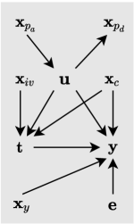
Figure 1: A possible causal graph of unobserved confounding.

Identification of TEs means that, the true observational distribution uniquely determines and gives the ATE or, better, CATE. Adapting standard identification results (Rubin, 2005)(Hernan and Robins, 2020, Ch. 3), we start with the following conditions, denoted by (A): there exists a (possibly unobserved) variable ${\mathbf{u}}\in\mathbb{R}^{n}$ such that together with ${\mathbf{x}}$, it gives (i) (Exchangeability) ${\mathbf{y}}(t)\raisebox{0.50003pt}{\rotatebox[origin={c}]{90.0}{$\models$}}{\textnormal{t}}|{\mathbf{u}},{\mathbf{x}}$ and (ii) (Overlap, or Positivity) $p({\textnormal{t}}|{\mathbf{u}},{\mathbf{x}})>0$; and (iii) (Consistency of counterfactuals) ${\mathbf{y}}={\mathbf{y}}(t)$ if ${\textnormal{t}}=t$. All of them are satisfied for both $t$, which is our convention when $t$ appears in a statement without quantification. Intuitively, exchangeability means all confounders are in essence contained in $({\mathbf{u}},{\mathbf{x}})$, and overlap means each possible value of $({\mathbf{u}},{\mathbf{x}})$ is observed for both treatment groups. Note that, joint exchangeability ${\mathbf{y}}(0),{\mathbf{y}}(1)\raisebox{0.50003pt}{\rotatebox[origin={c}]{90.0}{$\models$}}{\textnormal{t}}|{\mathbf{x}},{\mathbf{u}}$ is stronger than exchangeability and is not necessary for identification (Hernan and Robins, 2020, pp. 15).

A general example of causal structure that satisfies the three conditions is shown in Figure 1, although further structural constraints might be necessary for theoretical developments (see Sec. 4.4).. Here, ${\mathbf{x}}_{c}$,${\mathbf{x}}_{iv}$,${\mathbf{x}}_{p_{a}}$,${\mathbf{x}}_{p_{d}}$,${\mathbf{x}}_{y}$ are covariates that are: (observed) confounder, IV, antecedent proxy (that is antecedent of ${\mathbf{z}}$), descendant proxy, and antecedent of ${\mathbf{y}}$, respectively. The covariate(s) ${\mathbf{x}}$ may not have subsets in any categories in the graph. ${\mathbf{e}}$ is unobserved exogenous noise on ${\mathbf{y}}$. Assumption (A) may hold otherwise, e.g., ${\mathbf{x}}$ is a child of t.

CATE can be given by (2), using assumption (A) in the second equality.

$$\mu_{t}({\bm{x}})=\mathbb{E}(\mathbb{E}({\mathbf{y}}(t)|{\mathbf{u}},{\bm{x}}))=\mathbb{E}(\mathbb{E}({\mathbf{y}}|{\mathbf{u}},{\bm{x}},{\textnormal{t}}=t))=\textstyle\int(\int p(y|{\bm{u}},{\bm{x}},t)ydy)p({\bm{u}}|{\bm{x}})d{\bm{u}}.$$ (2)

If the variable ${\mathbf{u}}$ is observed, then (2) identifies CATE. However, if ${\mathbf{u}}$ is an unobserved confounder, the naive regression $\mathbb{E}[{\mathbf{y}}|{\mathbf{x}}={\bm{x}},{\mathbf{t}}=t]$ based on observable variables is not equal to $\mu_{t}({\bm{x}})$. In fact, if an unknown factor correlates with ${\mathbf{t}}$ positively and tends to give higher value for ${\mathbf{y}}$, the naive regression $\mathbb{E}[{\mathbf{y}}|{\mathbf{x}}={\bm{x}},{\mathbf{t}}=1]$ should be higher than $\mathbb{E}[{\mathbf{y}}(1)|{\mathbf{x}}={\bm{x}}]$.

2.2 Prognostic score

Our method models prognostic scores (Hansen, 2008), adapted as Pt-scores in this paper, closely related to the important concept of balancing score (Rosenbaum and Rubin, 1983). Both are sufficient scores for identification; prognostic scores are sufficient statistics of outcome predictors and balancing score is for the treatment (see Appendix B.1 for details).

Definition 2.1.

A Pt-score (PtS) is two functions $\mathbb{P}_{t}({\mathbf{u}},{\mathbf{x}})$ ($t=0,1$) such that ${\mathbf{y}}(t)\raisebox{0.50003pt}{\rotatebox[origin={c}]{90.0}{$\models$}}{\mathbf{u}},{\mathbf{x}}|\mathbb{P}_{t}({\mathbf{u}},{\mathbf{x}})$. A PtS is called a P-score (PS) if $\mathbb{P}_{0}=\mathbb{P}_{1}$.

The identity function is a trivial PS. If the true data generating process (DGP) satisfies additive noise model, i.e., ${\mathbf{y}}={\bm{f}}^{*}({\mathbf{u}},{\mathbf{x}},{\textnormal{t}})+{\mathbf{e}}$, then ${\bm{f}}^{*}_{t}$ is a PtS (Hansen, 2008); and it is a causal representation (Schölkopf et al., 2021) of the direct cause on ${\mathbf{y}}$, summarizing the effects of $({\mathbf{u}},{\mathbf{x}})$. The independence property of PtS (Lemma A.1 in Appendix),

$${\mathbf{y}}(t)\raisebox{0.50003pt}{\rotatebox[origin={c}]{90.0}{$\models$}}{\textnormal{t}},{\mathbf{u}},{\mathbf{x}}|\mathbb{P}_{t}({\mathbf{u}},{\mathbf{x}}),$$ (3)

is used in second equality of (4) in Theorem 2.2 which extends Proposition 5 in Hansen (2008).

Theorem 2.2 (CATE by PtS).

If $\mathbb{P}_{t}$ is a PtS, then CATE can be given by

$$\begin{split}\mu_{t}({\bm{x}})&=\mathbb{E}(\mathbb{E}({\mathbf{y}}({t})|\mathbb{P}_{t}({\mathbf{u}},{\bm{x}}),{\bm{x}}))=\mathbb{E}(\mathbb{E}({\mathbf{y}}|\mathbb{P}_{t}({\mathbf{u}},{\bm{x}}),{t}))\\ &=\textstyle\int(\int p_{{\mathbf{y}}|\mathbb{P}_{t},{\textnormal{t}}}(y|P,{t})ydy)p_{\mathbb{P}_{t}|{\mathbf{x}}}(P|{\bm{x}})dP,\end{split}$$ (4)

where ${\mathbf{y}}|\mathbb{P}_{t}({\mathbf{u}},{\mathbf{x}}),{\textnormal{t}}\sim p_{{\mathbf{y}}|\mathbb{P}_{t},{\textnormal{t}}}({\bm{y}}|P,t)$ and $\mathbb{P}_{t}({\mathbf{u}},{\mathbf{x}})|{\mathbf{x}}\sim p_{\mathbb{P}_{t}|{\mathbf{x}}}(P|{\bm{x}})$.

Compared to (2), $P=\mathbb{P}_{t}({\bm{u}},{\bm{x}})$ plays the role of ${\bm{u}}$, and $p_{{\mathbf{y}}|\mathbb{P}_{t},{\textnormal{t}}}$ conditions on $P$ instead of $({\bm{u}},{\bm{x}})$. In general, information from ${\mathbf{u}}$ is needed to determine $p_{{\mathbf{y}}|\mathbb{P}_{t},{\textnormal{t}}}$ and $p_{\mathbb{P}_{t}|{\mathbf{x}}}$. In Sec. 4, we first show that our generative model can identify an equivalent PS if ${\mathbf{u}}$ is observed (Sec. 4.2), and then discuss how our model is connected to and might learn relaxations of PtS when ${\mathbf{u}}$ is unobserved (Sec. 4.4).

3 Intact-VAE

In this section, we first introduce our generative model and VAE architecture, then prove the identifiability of the model, and finally use our model to estimate TEs. Our method is expected to learn a latent representation sufficient for TE identification/estimation, as we will see in the next section.

3.1 Model and architecture

We build the generative model (5) of our VAE with the direct cause $\mathbb{P}_{t}({\mathbf{u}},{\mathbf{x}})$ as the latent variable ${\mathbf{z}}$ and connect the model to iVAE. The outcome distribution $p_{{\mathbf{y}}|\mathbb{P}_{t},{\textnormal{t}}}$ in (4) is modeled by $p_{{\bm{f}}}({\bm{y}}|{\bm{z}},t)$, and the score distribution $p_{\mathbb{P}_{{\textnormal{t}}}|{\mathbf{x}}}$ in (4) is modeled by $p_{\bm{\lambda}}({\bm{z}}|{\bm{x}},t)$. The condition on ${\mathbf{x}}$ in the joint model $p({\mathbf{y}},{\mathbf{z}}|{\mathbf{x}},{\textnormal{t}})$ reflects that our estimand is CATE given ${\mathbf{x}}$.

$$\begin{gathered}p_{{\bm{\theta}}}({\bm{y}},{\bm{z}}|{\bm{x}},t)=p_{{\bm{f}}}({\bm{y}}|{\bm{z}},t)p_{\bm{\lambda}}({\bm{z}}|{\bm{x}},t),\\ p_{{\bm{f}}}({\bm{y}}|{\bm{z}},t)=p_{\bm{\epsilon}}({\bm{y}}-{\bm{f}}_{t}({\bm{z}})),\quad p_{\bm{\lambda}}({\bm{z}}|{\bm{x}},t)\sim\mathcal{N}({\bm{z}};{\bm{h}}_{t}({\bm{x}}),\operatorname{diag}({\bm{k}}_{t}({\bm{x}}))),\end{gathered}$$ (5)

The outcome assumes an additive noise model such that $\bm{\epsilon}\sim p_{\bm{\epsilon}}$ denotes the exogenous noise; and $p_{\bm{\lambda}}$ is a factorized Gaussian, where $\bm{\lambda}_{{\textnormal{t}}}({\mathbf{x}})\coloneqq\operatorname{diag}^{-1}({\bm{k}}_{{\textnormal{t}}}({\mathbf{x}}))({\bm{h}}_{{\textnormal{t}}}({\mathbf{x}}),-\frac{1}{2})^{T}$ is the natural parameter as in the exponential family. ${\bm{\theta}}\coloneqq({\bm{f}},\bm{\lambda})=({\bm{f}},{\bm{h}},{\bm{k}})$ contains the functional parameters.

The model is learned by the evidence lower bound (ELBO) which estimates the variational lower bound (See Appendix B.2 for the basics of VAEs):

$$\begin{split}\log p({\bm{y}}|{\bm{x}},t)\geq\log p({\bm{y}}|{\bm{x}},t)-D_{\mathrm{KL}}(q({\bm{z}}|{\bm{x}},{\bm{y}},t)\|p({\bm{z}}|{\bm{x}},{\bm{y}},t))\\ =\mathbb{E}_{{\bm{z}}\sim q}\log p_{{\bm{f}}}({\bm{y}}|{\bm{z}},t)-D_{\mathrm{KL}}(q({\bm{z}}|{\bm{x}},{\bm{y}},t)\|p_{\bm{\lambda}}({\bm{z}}|{\bm{x}},t)).\end{split}$$ (6)

with $p_{{\bm{f}}}$ as the decoder, $q$ as the encoder, and $p_{\bm{\lambda}}$ as the conditional prior.

Figure 2: Decoders of CVAE, iVAE, and Intact-VAE.

We name this architecture Intact-VAE (Identifiable treatment-conditional VAE). Note that (5) has a similar factorization with the generative model of iVAE, $p_{\bm{\theta}}({\bm{y}},{\bm{z}}|{\bm{x}})=p_{{\bm{f}}}({\bm{y}}|{\bm{z}})p_{\bm{\lambda}}({\bm{z}}|{\bm{x}})$; the first factor (decoder) does not condition on ${\mathbf{x}}$. Similarly, our decoder $p_{{\bm{f}}}({\bm{y}}|{\bm{z}},t)$ conditions on ${\mathbf{z}}$ as a PtS which satisfies ${\mathbf{y}}\raisebox{0.50003pt}{\rotatebox[origin={c}]{90.0}{$\models$}}{\mathbf{x}}|{\mathbf{z}},{\textnormal{t}}$. On the other hand, the condition on t is in both the factors of (5). Thus, our VAE architecture can be seen as a combination of iVAE and conditional VAE (CVAE) (Sohn et al., 2015; Kingma et al., 2014), with t as the conditioning variable. See Figure 2 for the comparison in terms of graphical models. Our encoder $q$, which conditions on all the observables and builds the approximate posterior, is similar to other VAEs. See Appendix B.2 for summary of CVAE and iVAE.

Though our theory allows more general distributions, for tractable inference and easy implementation, we have used factorized Gaussian for the prior, and now also use it for the decoder $p_{{\bm{f}},{\bm{g}}}({\bm{y}}|{\bm{z}},t)$ and encoder $q_{\bm{\phi}}({\bm{z}}|{\bm{x}},{\bm{y}},t)$; i.e., they are products of univariate Gaussian distributions:

$$\textstyle{\mathbf{y}}|{\mathbf{z}},{\textnormal{t}}\sim\prod_{j}^{d}\mathcal{N}(y_{j};f_{j},g_{j}),\quad{\mathbf{z}}|{\mathbf{x}},{\mathbf{y}},{\textnormal{t}}\sim\prod_{i=1}^{n}\mathcal{N}(z_{i};r_{i},s_{i}).$$ (7)

$\bm{\phi}\coloneqq({\bm{r}},{\bm{s}})$, like $\bm{\theta}$, contains functional parameters given by NNs which take $({\mathbf{x}},{\mathbf{y}},{\textnormal{t}})$ as inputs. We often write $t$ of the function argument in subscripts.

3.2 Identifiability of model parameters

Our model identifiability lays the foundation for principled causal effect estimation, as we will discuss in Sec. 4. The main theoretical result of iVAE is extended in our Theorem 3.1 which combines the techniques from Khemakhem et al. (2020a) and Sorrenson et al. (2019). Essentially the same results can be proved for other exponential family priors.

Theorem 3.1 (Model identifiability).

Given $p_{{\bm{\theta}}}({\bm{y}},{\bm{z}}|{\bm{x}},t)$ specified by (5) , for ${\textnormal{t}}=t$, assume

1. ${\bm{f}}_{t}({\mathbf{z}})$ is injective and differentiable;

2. there exist $2n+1$ points ${\bm{x}}_{0},...,{\bm{x}}_{2n}$ such that the $2n$-square matrix ${\bm{L}}_{t}\coloneqq[\bm{\gamma}_{t,1},...,\bm{\gamma}_{t,2n}]$ is invertible, where $\bm{\gamma}_{t,k}\coloneqq\bm{\lambda}_{t}({\bm{x}}_{k})-\bm{\lambda}_{t}({\bm{x}}_{0})$.

Then, given ${\textnormal{t}}=t$, the family is identifiable up to an equivalence class. That is, if $p_{{\bm{\theta}}}({\mathbf{y}}|{\mathbf{x}},{\textnormal{t}}=t)=p_{{\bm{\theta}}^{\prime}}({\mathbf{y}}|{\mathbf{x}},{\textnormal{t}}=t)$, we have the relation between parameters: for any ${\bm{y}}_{t}$ in the image of ${\bm{f}}_{t}$,

$${\bm{f}}_{t}^{-1}({\bm{y}}_{t})=\operatorname{diag}({\bm{a}}){{\bm{f}}^{\prime}_{t}}^{-1}({\bm{y}}_{t})+{\bm{b}}=:\mathcal{A}_{t}({{\bm{f}}^{\prime}_{t}}^{-1}({\bm{y}}_{t}))$$ (8)

where $\operatorname{diag}({\bm{a}})$ is an invertible $n$-diagonal matrix and ${\bm{b}}$ is a $n$-vector, both depend on $\bm{\lambda}_{t}$ and $\bm{\lambda}^{\prime}_{t}$.

The essence of Theorem 3.1 is ${\bm{f}}^{\prime}_{t}={\bm{f}}_{t}\circ\mathcal{A}_{t}$, that is, ${\bm{f}}_{t}$ can be identified (learned) up to an affine transformation defined by $\bm{\lambda}_{t}$. This identifiability of parameters does not directly imply TE identification; other assumptions are needed, as we show in Sec. 4. The assumptions in Theorem 3.1 are inherited from iVAE. Injectivity in i) is related to TE identification (Theorem 4.1), which requires injectivity in the true DGP and identifies a PtS up to an injective mapping. Intuitively, if ii) does not hold, then the support of $\bm{\lambda}({\mathbf{x}})$ degenerates to a $(2n-1)$-dimensional space; thus, ii) holds easily in practice (see B.2.3 in Khemakhem et al. (2020a)). Note that, to have (8), we only need the same observational distribution $p({\mathbf{y}}|{\mathbf{x}},{\textnormal{t}}=t)$, but this leaves room for different latent distributions.

3.3 Causal effect estimation

Once the VAE is learned by the ELBO (6), the estimate of $\mu_{t}$ is given by

$$\hat{\mu}_{\hat{t}}({\bm{x}})=\mathbb{E}_{q({\bm{z}}|{\bm{x}})}{\bm{f}}_{\hat{t}}({\bm{z}})=\mathbb{E}_{\mathcal{D}|{\bm{x}}\sim p({\bm{y}},t|{\bm{x}})}\mathbb{E}_{{\bm{z}}\sim q_{\bm{\phi}}}{\bm{f}}_{\hat{t}}({\bm{z}}),{\hat{t}}\in\{0,1\},$$ (9)

where $q({\bm{z}}|{\bm{x}})\coloneqq\mathbb{E}_{p({\bm{y}},t|{\bm{x}})}q_{\bm{\phi}}({\bm{z}}|{\bm{x}},{\bm{y}},t)$ is the aggregated posterior. Our overall algorithm steps should be clear. After training Intact-VAE by (6), we feed $({\bm{x}},{\bm{y}},t)$ into the encoder and draw posterior sample from it. Then, setting ${\textnormal{t}}=\hat{t}$ in the decoder, feed the posterior sample into it, we get counterfactual sample as outputs of the decoder. Finally, we infer CATE $\hat{\tau}({\bm{x}})=\hat{\mu}_{1}({\bm{x}})-\hat{\mu}_{0}({\bm{x}})$.

Our method also addresses the problem of imbalance–if $p({\mathbf{x}}|0),p({\mathbf{x}}|1)$ are very different for some ${\bm{x}}$, then we have few data points for one of $\mathcal{D}|{\bm{x}},t\coloneqq\{({\bm{x}},{\mathbf{y}},t)\}$, resulting in poor estimation. We set $\bm{\lambda}_{0}=\bm{\lambda}_{1}$ in the prior, and thus $p_{\bm{\lambda}}({\mathbf{z}}|{\mathbf{x}},{\textnormal{t}})=p_{\bm{\lambda}}({\mathbf{z}}|{\mathbf{x}})$ is independent of t given ${\mathbf{x}}$. The same prior for the treatment groups, i.e., the balanced prior of latent representation, is similar to balanced representation learning (Johansson et al., 2016; Shalit et al., 2017), where balanced representation is favored by ad hoc regularization. This is also related to the fact that, when building CVAE, unconditional prior can achieve better performance (Kingma et al., 2014).

By taking ${\mathbf{y}}$, the posterior model (the encoder) is better than the prior. On the other hand, sampling posterior requires post-treatment observation ${\bm{y}}$. Often, it is desirable that we can also have pre-treatment prediction for a new subject, with only the observation of its covariate ${\mathbf{x}}={\bm{x}}$. To this end, in (9), we use conditional prior $p({\mathbf{z}}|{\mathbf{x}})$ as a pre-treatment predictor for ${\mathbf{z}}$: draw sample from $p({\mathbf{z}}|{\bm{x}})$ instead of $q$ and get rid of the outer average taken on $\mathcal{D}$; all the others remain the same.

As usual, we expect the variational inference and optimization procedure to be (near) optimal; that is, the consistency of VAE. Consistent estimation using the prior is a direct corollary of TE identification and the consistent VAE. See Appendix A for formal statements and proofs. It is possible to prove the consistency of the posterior estimation, as shown in Bonhomme and Weidner (2021); Liao and Jiang (2011), and we leave this for future work, see Sec. 4.4.

4 Principled causal effect estimation via VAEs: retrospect and prospect

In this section, we present a critical review of existing VAE-based methods in Sec. 4.1 and then discuss theoretical developments that can lead to principled causal estimation, under different settings.

4.1 VAEs for TE estimation

Most VAE methods for TEs, e.g., Louizos et al. (2017); Zhang et al. (2020); Vowels et al. (2020); Lu et al. (2020), add ad hoc heuristics into the VAEs, and thus break down probabilistic modeling, not to mention model identifiability. Moreover, the methods learn representations from proxy variables, leading to either impractical assumptions or conceptual inconsistency, in TE identification.

On identification. First, as to TE identification, CEVAE assumes unobserved confounder can be recovered, which is rarely possible even under further structural assumptions (Tchetgen et al., 2020). Indeed, Rissanen and Marttinen (2021) recently give evidence that the method often fails. Other methods (Zhang et al., 2020; Vowels et al., 2020; Lu et al., 2020) assume unconfoundedness but still rely on proxy at least intuitively; for example, Lu et al. (2020) factorize the decoder as if in the proxy setting. However, unconfoundedness and proxy should not be put together. The conceptual inconsistency is that, by definition, unconfoundedness means covariates fully control confounding, while the motivation for proxy is that unconfoundedness is often not satisfied in practice and covariates are at best proxies of confounding, which are non-confounders causally connected to confounders (Tchetgen et al., 2020). Second, without model identifiability, the empirical results of the methods lack solid ground; under settings not covered by their experiments, the methods would silently fail to learn proper representations, as we show in Sec. 5.1.

On ad hoc heuristics. Ad hoc heuristics break down probabilistic modeling and/or give ELBOs that do not optimally estimate the models. For example, in CEVAE, $q({\textnormal{t}}|{\mathbf{x}})$ and $q({\mathbf{y}}|{\mathbf{x}},{\textnormal{t}})$ are added into the encoder to have pre-treatment estimation, and the ELBO has two additional likelihood terms respectively. The VAE in Zhang et al. (2020) is even more ad hoc; it splits the latent variable ${\mathbf{z}}$ into three components, and applies the ad hoc tricks of CEVAE to each of the component. Particularly, when constructing the encoder, they implicitly assume the three components of ${\mathbf{z}}$ are conditional independent give ${\mathbf{x}}$, which violates the intended graphical model.

Compared to the above methods, our Intact-VAE is simpler and more principled, and often has better performance. It models a prognostic score as the latent variable and is based on the identification equation (4), while not compromised by ad hoc heuristics. Our ELBO is derived by standard variational lower bound (6). Moreover, our pre-treatment prediction is given naturally by the prior, thanks to the correspondence between our model and (4). We show in the following subsections how our model and its identifiability inspire theoretical developments in TE identification.

4.2 Identification under unconfoundedness

As a first step, we take up theoretical analysis of Intact-VAE under assumption (A) when ${\mathbf{u}}$ is observed (i.e., ${\mathbf{u}}$ is components of ${\mathbf{x}}$). Then, we have ${\mathbf{y}}(t)\raisebox{0.50003pt}{\rotatebox[origin={c}]{90.0}{$\models$}}{\textnormal{t}}|{\mathbf{x}}$ and $p({\textnormal{t}}|{\mathbf{x}})>0$ (Exchangeability and Overlap given ${\mathbf{x}}$). This is the standard unconfoundedness setting. Regarding to the PtS, $p_{\mathbb{P}_{{\textnormal{t}}}|{\mathbf{x}}}$ in (4) degenerates to $\mathbb{P}_{{\textnormal{t}}}({\mathbf{x}})$. Theorem 4.1 is an identification under shape restriction (Chetverikov et al., 2018), because injectivity in assumption i) is monotonicity if ${\bm{j}}_{t}$ is on $\mathbb{R}$.

Theorem 4.1 (Identification via PS).

Use model (5) under unconfoundedness, further assume

1. (Injective separation) $\mu_{t}({\mathbf{x}})={\bm{j}}_{t}(\mathbb{O}({\mathbf{x}}))$ for some function $\mathbb{O}$ and injective function ${\bm{j}}_{t}$;

2. (Score matching) in the model, $n=d$, ${\bm{f}}_{t}$ is injective, ${\bm{h}}_{0}({\mathbf{x}})={\bm{h}}_{1}({\mathbf{x}})$, and ${\bm{k}}({\mathbf{x}})=\bm{0}$.

Then, if $\mathbb{E}_{p_{\bm{\theta}}}({\mathbf{y}}|{\mathbf{x}},{\textnormal{t}})=\mathbb{E}({\mathbf{y}}|{\mathbf{x}},{\textnormal{t}})$, we have

1. (Recovery of score) ${\mathbf{z}}_{\bm{\lambda},t}={\bm{h}}_{t}({\mathbf{x}})={\bm{v}}(\mathbb{O}({\mathbf{x}}))$ where ${\bm{v}}$ is an injective function;

2. (CATE Identification) $\mu_{{t}}({\mathbf{x}})=\hat{\mu}_{{t}}({\mathbf{x}})\coloneqq\mathbb{E}_{p_{\bm{\lambda}}({\mathbf{z}}|{\mathbf{x}},t)}\mathbb{E}_{p_{{\bm{f}}}}({\mathbf{y}}|{\mathbf{z}},{t})={\bm{f}}_{t}({\bm{h}}_{t}({\mathbf{x}}))$.

In essence, $\mu_{t}$ is identified up to an invertible mapping ${\bm{v}}$, such that ${\bm{f}}_{t}={\bm{j}}_{t}\circ{\bm{v}}^{-1}$ and ${\bm{h}}_{t}={\bm{v}}\circ\mathbb{O}$, with same ${\bm{v}}$ for both $t$. The connection to PS is clear; if additive noise model is the ground truth, then $\mathbb{O}$ is a PS because $\mu_{t}$ is is a PtS. Then, because $\mathbb{O}$ is recovered up to ${\bm{v}}$, the independence ${\mathbf{y}}(t)\raisebox{0.50003pt}{\rotatebox[origin={c}]{90.0}{$\models$}}{\mathbf{x}}|\mathbb{O}({\mathbf{x}})$ is preserved. Assumption i) says that the treatment affects $\mathbb{E}({\mathbf{y}}|{\bm{x}})$ only through injective ${\bm{j}}_{t}$ (which is identified up to ${\bm{v}}$), and CATEs are given by $\mu_{0}$ and an invertible function ${\bm{i}}\coloneqq{\bm{j}}_{1}\circ{\bm{j}}_{0}^{-1}$. See Appendix C for real-world examples satisfying i) and the connection to “independent causal mechanisms” (Janzing and Scholkopf, 2010). With the existence of $\mathbb{O}$, Assumption ii) simply matches the model to the truth. Note that, with ${\bm{k}}({\mathbf{x}})=\bm{0}$, the prior ${\mathbf{z}}_{\bm{\lambda},t}\sim p_{\bm{\lambda}}({\bm{z}}|{\bm{x}},t)$ degenerates to function ${\bm{h}}_{t}({\mathbf{x}})$.

Interestingly, Theorem 4.1 does not depend on Theorem 3.1, mainly because i) is strong in the sense that it indicates a PS. To work under general additive noise models with only PtSs, we use our model identifiability (8) in Anonymous (2021), the main ideas of which is briefly summarized below.

4.3 Identification without overlap of ${\mathbf{x}}$

The advantage of PtS can be more clearly seen when ${\mathbf{x}}$ does not satisfy overlap. Now, a straightforward estimation of TEs is not possible at a non-overlapping value ${\bm{x}}$ due to lack of data. However, $\mathbb{P}_{t}({\mathbf{x}})$ can map some non-overlapping values to an overlapping value, and overlap of $\mathbb{P}_{t}({\mathbf{x}})$ implies but is not implied by overlap of ${\mathbf{x}}$ (D’Amour et al., 2020). In a parallel submission (Anonymous, 2021), we assume the overlap of a PtS instead and extend Theorem 4.1 to this limited overlap setting. This is a natural next step, because we already model a PtS as the latent variable.

A main result of Anonymous (2021) is that the latent variable of our VAE recovers a PtS and identifies the CATE through the model, under limited overlap, similar to the conclusion 1) and 2) in Theorem 4.1. To recover the PtS, we derive a condition and strengthen (8) so that $\mathcal{A}_{0}=\mathcal{A}_{1}$, which compensates for $\mathbb{P}_{0}\neq\mathbb{P}_{1}$. Thus, we fully exploit the probabilistic nature of VAE in modeling, and give principled causal estimation based on the identifiability of VAE.

Still, with ${\mathbf{u}}$ observed, it would seem unnecessary to model $\mathbb{P}_{{\textnormal{t}}}({\mathbf{x}})$ by the distribution $p_{\bm{\lambda}}({\bm{z}}|{\bm{x}},t)$ (the prior). However, the prior, together with the encoder, quantifies the uncertainty of scores–we are uncertain how likely a PS (not only a PtS) can be recovered (Anonymous, 2021, Sec. 4.1 & C.5).

4.4 Preliminary thoughts under unobserved confounding

The positive experimental results motivate us to consider the theory under unobserved confounding. Moreover, the prior in (5) is even more natural with ${\mathbf{u}}$ unobserved, since $p_{\mathbb{P}_{{\textnormal{t}}}|{\mathbf{x}}}$ is not degenerated due to the uncertainty of ${\mathbf{u}}$. Thus, we conjecture that, in our VAE framework, unobserved confounding is treated as a source of uncertainty of scores and is handled in a Bayesian way. We give more considerations for future theoretical work below.

Identification. Auxiliary structures (e.g., IVs) can give TE identifications via control functions $\mathbb{C}({\textnormal{t}},{\mathbf{x}})$, conditioning on which the treatment becomes exogenous, that is, ${\mathbf{y}}(t)\raisebox{0.50003pt}{\rotatebox[origin={c}]{90.0}{$\models$}}{\textnormal{t}}|\mathbb{C}(t,{\mathbf{x}})$ (Matzkin, 2007; Wooldridge, 2015). Control functions can be stochastic, as in Puli and Ranganath (2020). Consistent TE estimation can be given by a regression of outcome on the treatment and a control function. Our model (5) can be seen as a two-stage procedure: first, $p_{\bm{\lambda}}({\bm{z}}|{\bm{x}},t)$ gives a stochastic control function; second, $p_{{\bm{f}}}({\bm{y}}|{\bm{z}},t)$ regresses the outcome. We need to specify the control function learned by Intact-VAE and the required structural constraints. Control functions are recently found under the proxy setting (Nagasawa, 2021), or in the presence of both proxies and IVs (Tien, 2021).

Estimation. In causal inference, many models, including nonparametric IV regression (NPIV), are stated as conditional moment restrictions (CMRs) (Newey, 1993). Optimizing the ELBO of our VAE, given by (6), can be seen as finding functions ${\bm{f}}$ and $\mathbb{C}$, subject to the CMR $\mathbb{E}_{p_{\bm{\theta}}}({\mathbf{y}}|{\mathbf{x}},{\textnormal{t}})=\mathbb{E}({\mathbf{y}}|{\mathbf{x}},{\textnormal{t}})$. We believe our Intact-VAE framework, possibly with modifications, can be shown to give optimal estimation under the CMR. There are formal connections between CMRs and quasi-Bayesian analysis using KL divergence (Zhang, 2006; Jiang and Tanner, 2008; Kim, 2002). For example, Kato (2013) uses a quasi-likelihood from the CMR of NPIV to set the prior, and the Gibbs posterior (Zhang, 2006; Jiang and Tanner, 2008) is a minimizer of an information complexity which has a variational characterization similar to an ELBO. For general CMR models, Liao and Jiang (2011) extend Kim (2002) and give the best approximation to the true likelihood function under the CMR by minimizing a KL divergence. Very recently, Wang et al. (2021) employ quasi-Bayesian analysis to kernel-based IV methods, but only consider unconditional moments.

5 Experiments

We use the proposed Intact-VAE for three types of data, and compare it with existing methods.

Unless otherwise indicated, for each function ${\bm{f}},{\bm{g}},{\bm{h}},{\bm{k}},{\bm{r}},{\bm{s}}$ in our VAE, we use a multilayer perceptron (MLP) that has 3*200 hidden units with ReLU activation, and $\bm{\lambda}=({\bm{h}},{\bm{k}})$ depends only on ${\mathbf{x}}$. The Adam optimizer with initial learning rate $10^{-4}$ and batch size 100 is employed. All experiments use early-stopping of training by evaluating the ELBO on a validation set. We test post-treatment results on training and validation set jointly. The treatment and (factual) outcome should not be observed for pre-treatment predictions, so we report them on a testing set. More details on hyper-parameters and settings are given in each experiment and Appendix.

As in previous works (Shalit et al., 2017; Louizos et al., 2017), we report the absolute error of ATE $\epsilon_{ate}\coloneqq|\mathbb{E}_{\mathcal{D}}(y(1)-y(0))-\mathbb{E}_{\mathcal{D}}\hat{\tau}({\bm{x}})|$, and the square root of empirical PEHE (Hill, 2011) $\epsilon_{pehe}\coloneqq\mathbb{E}_{\mathcal{D}}((y(1)-y(0))-\hat{\tau}({\bm{x}}))^{2}$ for individual-level TEs.

5.1 Synthetic dataset

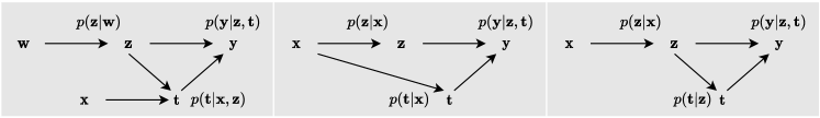
Figure 3: Graphical models for generating synthetic datasets. From left: IV ${\mathbf{x}}$, ignorability given ${\mathbf{x}}$, and proxy ${\mathbf{x}}$. Note that in the latter two cases, reversing the arrow between ${\mathbf{x}},{\mathbf{z}}$ does not change any independence relationships, and causal interpretations of the graphs remain the same.

$$\begin{split}\textstyle{\mathbf{x}}\sim\mathcal{N}(\bm{\mu},\bm{\sigma});{\textnormal{z}}|{\mathbf{x}}\sim\mathcal{N}(h({\mathbf{x}}),\beta k({\mathbf{x}}));{\textnormal{t}}|{\mathbf{x}},{\textnormal{z}}\sim\operatorname{Bern}(\operatorname{Logi}(l({\mathbf{x}},{\textnormal{z}})));{\mathbf{y}}|{\textnormal{z}},{\textnormal{t}}\sim\mathcal{N}(f({\textnormal{z}},{\textnormal{t}}),\alpha).\end{split}$$ (10)

We generate synthetic datasets by (10). The parameters are different between DGPs: $\mu_{i}$ and $\sigma_{i}$ are randomly generated; the functions $h,k,l$ are linear with random coefficients; and $f_{0},f_{1}$ is built by separated randomly initialized (then fixed) NNs. We generate two kinds of outcome models, depending on the type of $f$: linear and nonlinear outcome models use random linear functions and NNs with invertible activations and random weights, respectively. We set the outcome and proxy noise level by $\alpha,\beta$ respectively. See Appendix E.1 for more details.

We experiment on three different causal structures as shown in graphical models of Figure 3, by variation on (10). Instead of taking inputs ${\mathbf{x}},{\textnormal{z}}$ in $l$, we consider two special cases: $l\coloneqq l({\mathbf{x}})$, then ${\mathbf{x}}$ fully adjusts for confounding, we are in fact unconfounded; and $l\coloneqq l({\textnormal{z}})$, then we have unobserved confounder z and proxy ${\mathbf{x}}$ of z. To introduce ${\mathbf{x}}$ as instrumental variable, we generate another 1-dimensional random source w in the same way as ${\mathbf{x}}$, and use w instead of ${\mathbf{x}}$ to generate ${\textnormal{z}}|{\textnormal{w}}\sim\mathcal{N}(h({\textnormal{w}}),\beta k({\textnormal{w}}))$; except indicated above, other aspects of the models are specified by (10).

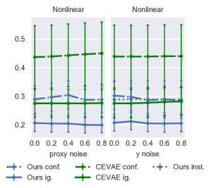
Figure 4: Pre-treatment $\sqrt{\epsilon_{pehe}}$ on nonlinear synthetic dataset. Error bar on 100 random DGPs. We adjust one of the noise levels $\alpha,\beta$ in each panel, with another fixed to 0.2.

For each causal structure, and with the same kind of outcome models, and the same noise levels ($\alpha,\beta$), we evaluate Intact-VAE and CEVAE on 100 random DGPs, with different sets of parameters in (10). For each DGP, we sample 1500 data points, and split them into 3 equal sets for training, validation, and testing. Both the methods use 1-dimensional latent variable in VAE. For fair comparison, all the hyper-parameters, including type and size of NNs, learning rate, and batch size, are the same for both the methods.

Figure 4 shows our method significantly outperforms CEVAE on all cases Both methods work the best under unconfoundedness (“ig.”), as expected. The performances of our method on IV (“inst.”) and proxy (“conf.”) settings match that of CEVAE under unconfoundedness, showing the effective deconfounding. See Appendix E.1 for results on linear outcome. Results for ATE and post-treatment are similar.

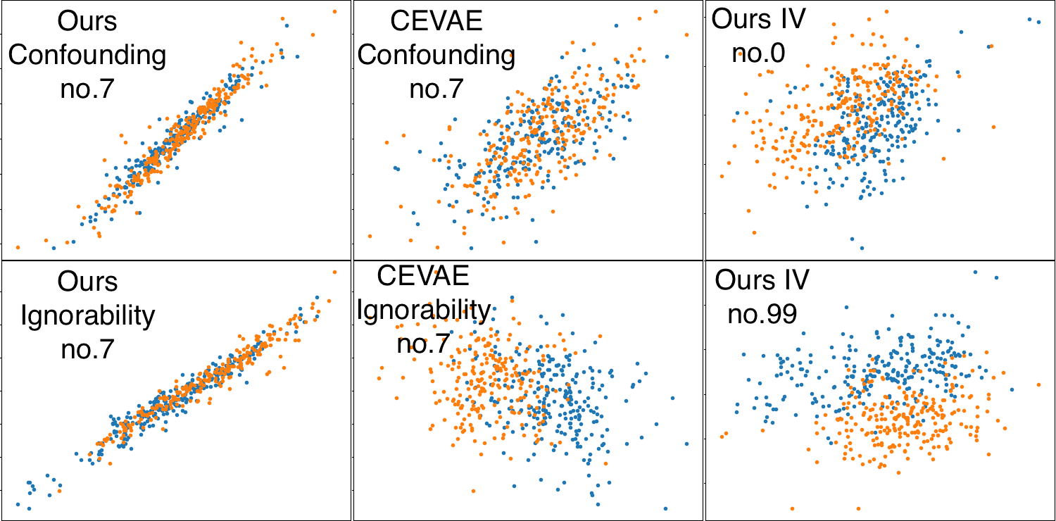
Figure 5: Plots of recovered - true latent on the nonlinear outcome. Blue: $t=0$, Orange: $t=1$. $\alpha,\beta=0.4$. “no.” indicates index among the 100 random models.

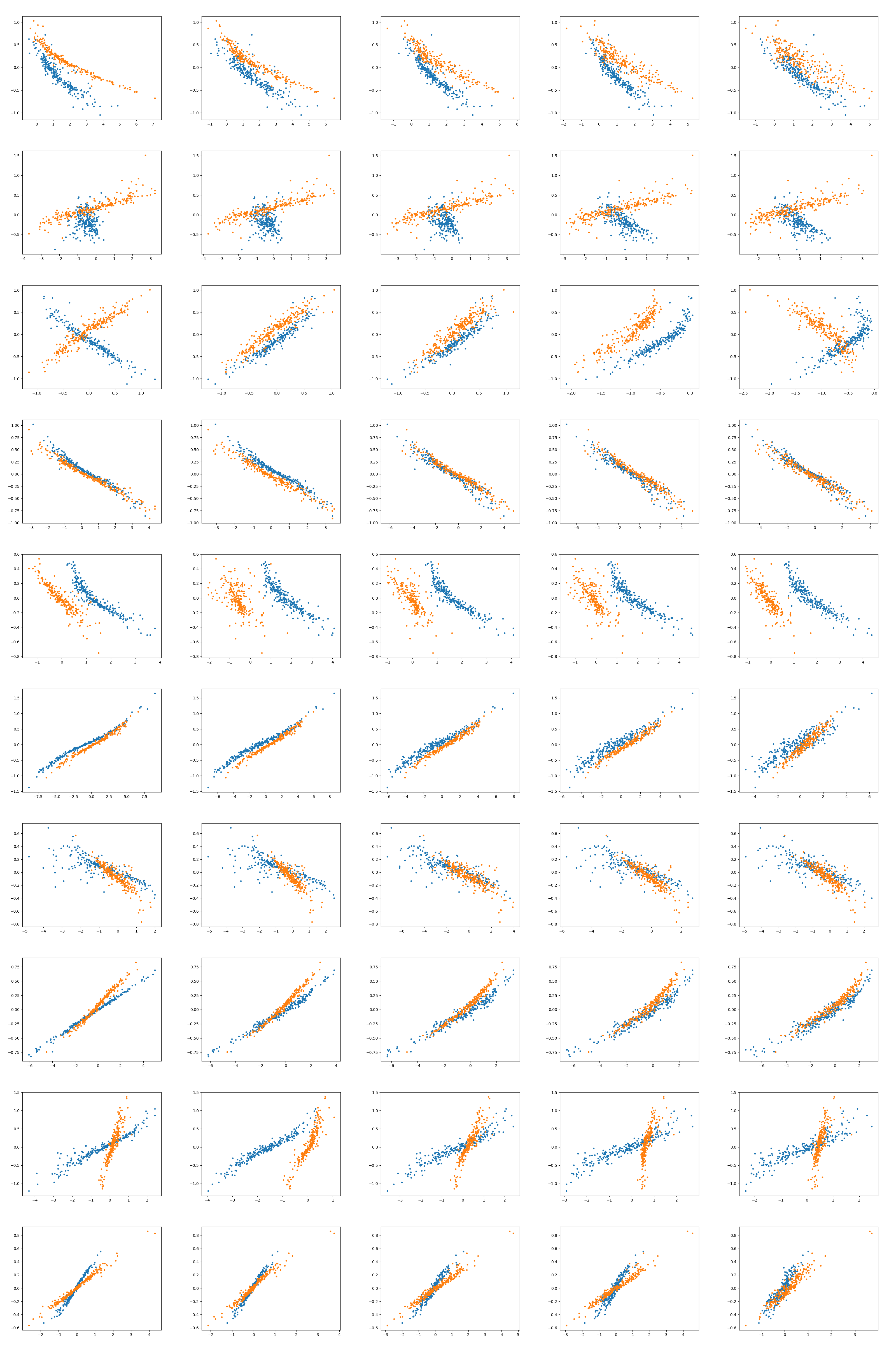
Figure 11: Plots of recovered-true latent when ignorability holds. Conditional prior depends on $t$. Rows: first 10 nonlinear random models, columns: outcome noise level. Compare to the previous figure, we can see the transformations for $t=0,1$ are not the same.

Here, the true latent z is a PS, and there are no better candidate PSs than z, because $f_{t}$ is invertible and no information can be dropped from z. Thus, as shown in Figure 5, our method learns representation as an approximate affine transformation of the true latent value, as a result of our model identifiability. More latent plots are in Appendix E.3 (the end of the paper). As expected, both recovery and estimation are better with unconditional prior $p({\textnormal{z}}|{\mathbf{x}})$, and we see examples of bad recovery using conditional $p({\textnormal{z}}|{\mathbf{x}},{\textnormal{t}})$ in Appendix Figure 11. CEVAE shows much lower quality of recovery, particularly with large noises. Under the IV setting, while TEs are estimated as well as for the proxy setting, the relationship to the true latent is significantly obscured, because the true latent is correlated to IV ${\mathbf{x}}$ only given t, while we model it by $p({\textnormal{z}}|{\mathbf{x}})$. This confirms that our method does not need to recover the true confounder distribution.

We see our method is robust to the unknown noise level. This indicates that noises are learned by our VAE. Appendix E.3 shows that the noise level affects how well we recover the latent variable.

5.2 IHDP benchmark dataset

This experiment shows our balanced estimator matches the state-of-the-art methods specialized for standard unconfoundedness. The IHDP dataset (Hill, 2011) is widely used to evaluate machine learning based causal inference methods, e.g. Shalit et al. (2017); Shi et al. (2019).

The generating process is as following (Hill, 2011, Sec. 4.1).

$${\textnormal{y}}(0)\sim\mathcal{N}(e^{{\bm{a}}^{T}({\mathbf{x}}+{\bm{b}})},1),\quad{\textnormal{y}}(1)\sim\mathcal{N}({\bm{a}}^{T}{\mathbf{x}}-o,1),$$ (11)

where ${\bm{b}}$ is constant with all elements equal to $0.5$, ${\bm{a}}$ and $o$ are a random parameters. Thus, it is not necessary to condition on ${\mathbf{x}}$, but the linear PS ${\bm{a}}^{T}{\mathbf{x}}$ is sufficient. See Appendix E.2 for more details.

To see our balancing property clearly, we add two components specialized for balancing from Shalit et al. (2017) into our method. First, we use two separate NNs to build the two outcome functions ${\bm{f}}_{t}({\mathbf{z}}),t=0,1$ in our model (5). Second, we add to our ELBO (6) a regularization term, which is the Wasserstein distance (Cuturi, 2013) between $\mathbb{E}_{\mathcal{D}\sim p({\mathbf{x}}|{\textnormal{t}}=t)}p_{\bm{\lambda}}({\mathbf{z}}|{\mathbf{x}}),t\in\{0,1\}$.

As shown in Table 1, Intact-VAE outperforms or matches the state-of-the-art methods. In particular, our method has the best ATE estimation; and it has the best individual-level estimation, adding the two components from Shalit et al. (2017). We can see in the caption of Table 1, the specialized additions do not really improve our method, only causing a tradeoff between CATE and ATE estimation, and this may due to the tradeoff between fitting and balancing. And notably, our method outperforms other generative models (CEVAE and GANITE) by large margins.

We find higher than 1-dimensional ${\mathbf{z}}$ in Intact-VAE gives better results, because we have discrete true PS due to the existence of discrete covariates. We report results with 10-dimensional latent variable. The robustness of VAE under model misspecification was also observed by Louizos et al. (2017), where they used 5-dimensional Gaussian latent variable to model a binary ground truth.

Table 1: Errors on IHDP. The mean and std are calculated over 1000 random data generating models. *Results with modifications are $\epsilon_{ate}=.31_{\pm.01}/.30_{\pm.01}$ and $\sqrt{\epsilon_{pehe}}=\textbf{.77}_{\pm.02}/\textbf{.69}_{\pm.02}$. Bold indicates method(s) that are significantly better than all the others. The results of the others are taken from Shalit et al. (2017), except GANITE (Yoon et al., 2018) and CEVAE (Louizos et al., 2017).

Method	TMLE	BNN	CFR	CF	CEVAE	GANITE	Ours*
$\epsilon_{ate}$	NA/.30±.01	.42±.03/.37±.03	.27±.01/.25±.01	.40±.03/.18±.01	.46±.02/.34±.01	.49±.05/.43±.05	$.31_{\pm.01}$/$.30_{\pm.01}$
$\sqrt{\epsilon_{pehe}}$	NA/5.0±.2	2.1±.1/2.2±.1	.76±.02/.71±.02	3.8±.2/3.8±.2	2.6±.1/2.7±.1	2.4±.4/1.9±.4	.77±.02/.69±.02

5.3 Pokec social network dataset

We show our method is the best compared with the methods specialized for networked deconfounding, a challenging problem in its own right. Pokec (Leskovec and Krevl, 2014) is a real world social network dataset. We experiment on a semi-synthetic dataset based on Pokec, introduced in Veitch et al. (2019), and use exactly the same pre-processing and generating procedure. The pre-processed network has about 79,000 vertexes (users) connected by 1.3 $\times 10^{6}$ undirected edges. The subset of users used here are restricted to three living districts that are within the same region. The network structure is expressed by binary adjacency matrix ${\bm{G}}$.

Each user has 12 attributes, among which district, age, or join date is used as a confounder z to build 3 different datasets, with remaining 11 attributes used as covariate ${\mathbf{x}}$. Treatment t and outcome ${\mathbf{y}}$ are synthesised as following:

$${\textnormal{t}}\sim\operatorname{Bern}(g({\textnormal{z}})),\quad{\mathbf{y}}={\textnormal{t}}+10(g({\textnormal{z}})-0.5)+\epsilon,\text{ where $\epsilon$ is standard normal. }$$ (12)

Note that district is of 3 categories; age and join date are also discretized into three bins. There is a PS that is $g({\textnormal{z}})$, which maps the three categories and values to $\{0.15,0.5,0.85\}$.

As in Veitch et al. (2019), we split the users into 10 folds, test on each fold and report the mean and std of pre-treatment ATE predictions. We further separate the rest of users (in the other 9 folds) by 6:3, for training and validation. Table 2 shows the results. In addition, the pre-treatment $\sqrt{\epsilon_{pehe}}$ for Age, District, and Join date confounders are 1.085, 0.686, and 0.699 respectively, practically the same as the ATE errors. Veitch et al. (2019) do not give individual-level prediction.

Table 2: Pre-treatment ATE on Pokec. Ground truth ATE is 1, as we can see in (12). “Unadjusted” estimates ATE by $\mathbb{E}_{\mathcal{D}}(y_{1})-\mathbb{E}_{\mathcal{D}}(y_{0})$. “Parametric” is a stochastic block model for networked data (Gopalan and Blei, 2013). “Embed-” denotes the best alternatives given by (Veitch et al., 2019). Bold indicates method(s) that are significantly better than all the others. 20-dimensional latent variable in Intact-VAE works better, and its result is reported. The results of the other methods are taken from (Veitch et al., 2019).

	Unadjusted	Parametric	Embed-Reg.	Embed-IPW	Ours
Age	4.34 $\pm$ 0.05	4.06 $\pm$ 0.01	2.77 $\pm$ 0.35	3.12 $\pm$ 0.06	2.08 $\pm$ 0.32
District	4.51 $\pm$ 0.05	3.22 $\pm$ 0.01	1.75 $\pm$ 0.20	1.66 $\pm$ 0.07	1.68 $\pm$ 0.10
Join Date	4.03 $\pm$ 0.06	3.73 $\pm$ 0.01	2.41 $\pm$ 0.45	3.10 $\pm$ 0.07	1.70 $\pm$ 0.13

Intact-VAE is expected to learn a PS from ${\bm{G}},{\mathbf{x}}$, if we can exploit the network structure effectively. Given the huge network structure, most users can practically be identified by their attributes and neighborhood structure, which means z can be roughly seen as a deterministic function of ${\bm{G}},{\mathbf{x}}$. This idea is comparable to Assumptions 2 and 4 in Veitch et al. (2019), which postulate directly that a balancing score can be learned in the limit of infinite large network.

To extract information from the network structure, we use Graph Convolutional Network (GCN) (Kipf and Welling, 2017) in the prior and encoder of Intact-VAE. Note that GCN cannot be trained by mini-batch, instead, we perform batch gradient decent using all data for each iteration, with initial learning rate $10^{-2}$. We use dropout (Srivastava et al., 2014) with rate 0.1 to prevent overfitting.

GCN need to take as inputs the network matrix ${\bm{G}}$ and the covariates matrix ${\bm{X}}\coloneqq({\bm{x}}_{1}^{T},\dotsc,{\bm{x}}_{M}^{T})^{T}$ of all users, where $M$ is user number, regardless of whether it is in training, validation, or testing phase; and it outputs a representation matrix ${\bm{R}}$, again for all users. To enable sample separation, we need to make sure the treatment and outcome are used only in the respective phase, e.g., $(y_{m},t_{m})$ of a testing user $m$ is only used in testing. During training, we select the rows in ${\bm{R}}$ that correspond to users in training set. Then, treat this training representation matrix as if it is the covariate matrix for a non-networked dataset, that is, the downstream networks in conditional prior and encoder are the same as in the other two experiments, except that they take $({\bm{R}}_{m,:})^{T}$ where ${\bm{x}}_{m}$ was expected as input. And we have respective selection operations for validation and testing. We can still train Intact-VAE including GCN by Adam, simply setting the gradients of non-seleted rows of ${\bm{R}}$ to 0.

6 Conclusion

In this work, we proposed Intact-VAE for CATE estimation. Our generative model is identifiable and has a sufficient score as its latent variable. Our method outperforms or matches state-of-the-art methods under diverse settings including unobserved confounding. In Sec. 4, we explained why the current VAE methods are unsatisfactory from a more “causal” viewpoint. We gave theoretical analysis of Intact-VAE under unconfoundedness and discussed parallel and future theoretical work–TE identification without overlap and approaches to identification and optimal estimation under unobserved confounding. We believe this series of work will also pave the way towards principled causal effect estimation by other deep architectures, given the fast advances in deep identifiable models. For example, recently, Khemakhem et al. (2020b) provide identifiability to deep energy models, and Roeder et al. (2021) extend the result to a wide class of state-of-the-art deep discriminative models. We hope this work will inspire other methods based on deep identifiable models.

Appendix A Proofs and additional theoretical results

Theorem 2.2 is rather straightforward from (3) (see Lemma A.1) and the definition of PtS, and thus its proof is omitted.

We give main properties of Pt-score as following.

Lemma A.1.

If ${\mathbf{v}}$ gives exchangeability, and $\mathbb{P}_{{\textnormal{t}}}({\mathbf{v}})$ is a Pt-score, then ${\mathbf{y}}(t)\raisebox{0.50003pt}{\rotatebox[origin={c}]{90.0}{$\models$}}{\mathbf{v}},{\textnormal{t}}|\mathbb{P}_{t}({\mathbf{v}})$.

The following three properties of conditional independence will be used repeatedly in proofs.

Proposition A.2 (Properties of conditional independence).

(Pearl, 2009, 1.1.55) For random variables ${\mathbf{w}},{\mathbf{x}},{\mathbf{y}},{\mathbf{z}}$. We have:

$$\begin{split}{\mathbf{x}}\raisebox{0.50003pt}{\rotatebox[origin={c}]{90.0}{$\models$}}{\mathbf{y}}|{\mathbf{z}}\land{\mathbf{x}}\raisebox{0.50003pt}{\rotatebox[origin={c}]{90.0}{$\models$}}{\mathbf{w}}|{\mathbf{y}},{\mathbf{z}}&\implies{\mathbf{x}}\raisebox{0.50003pt}{\rotatebox[origin={c}]{90.0}{$\models$}}{\mathbf{w}},{\mathbf{y}}|{\mathbf{z}}\text{ (Contraction)}.\\ {\mathbf{x}}\raisebox{0.50003pt}{\rotatebox[origin={c}]{90.0}{$\models$}}{\mathbf{w}},{\mathbf{y}}|{\mathbf{z}}&\implies{\mathbf{x}}\raisebox{0.50003pt}{\rotatebox[origin={c}]{90.0}{$\models$}}{\mathbf{y}}|{\mathbf{w}},{\mathbf{z}}\text{ (Weak union)}.\\ {\mathbf{x}}\raisebox{0.50003pt}{\rotatebox[origin={c}]{90.0}{$\models$}}{\mathbf{w}},{\mathbf{y}}|{\mathbf{z}}&\implies{\mathbf{x}}\raisebox{0.50003pt}{\rotatebox[origin={c}]{90.0}{$\models$}}{\mathbf{y}}|{\mathbf{z}}\text{ (Decomposition)}.\end{split}$$

Proof A.3 (of Lemma A.1).

From ${\mathbf{y}}(t)\raisebox{0.50003pt}{\rotatebox[origin={c}]{90.0}{$\models$}}{\textnormal{t}}|{\mathbf{v}}$ (exchangeability of ${\mathbf{v}}$), and since $\mathbb{P}_{t}$ is a function of ${\mathbf{v}}$, we have ${\mathbf{y}}(t)\raisebox{0.50003pt}{\rotatebox[origin={c}]{90.0}{$\models$}}{\textnormal{t}}|\mathbb{P}_{t}({\mathbf{v}}),{\mathbf{v}}$ (1).

From (1) and ${\mathbf{y}}(t)\raisebox{0.50003pt}{\rotatebox[origin={c}]{90.0}{$\models$}}{\mathbf{v}}|\mathbb{P}_{t}({\mathbf{v}})$ (definition of Pt-score), using contraction rule, we have
${\mathbf{y}}(t)\raisebox{0.50003pt}{\rotatebox[origin={c}]{90.0}{$\models$}}{\textnormal{t}},{\mathbf{v}}|\mathbb{P}_{t}({\mathbf{v}})$ for both $t$.

Apply the proposition to our setting, we have eq. (3).

In the proof of Theorem 3.1, all equations and variables should condition on $t$, and we omit the conditioning in notation for convenience.

The main part of our model identifiability follows from that of Theorem 1 in Khemakhem et al. (2020a), but now adapted to the dependency on $t$. Here we give an outline of the proof, and the details can be easily filled by referring to Khemakhem et al. (2020a).

Proof A.4 (of Theorem 3.1).

Using i) and ii) , we transform $p_{{\bm{f}},\bm{\lambda}}({\mathbf{y}}|{\mathbf{x}},t)=p_{{\bm{f}}^{\prime},\bm{\lambda}^{\prime}}({\mathbf{y}}|{\mathbf{x}},t)$ into equality of noiseless distributions, that is,

$$q_{{\bm{f}}^{\prime},\bm{\lambda}^{\prime}}({\mathbf{y}})=q_{{\bm{f}},\bm{\lambda}}({\mathbf{y}})\coloneqq p_{\bm{\lambda}}({\bm{f}}^{-1}({\mathbf{y}})|{\mathbf{x}},t)vol({\bm{J}}_{{\bm{f}}^{-1}}({\mathbf{y}}))\mathbb{I}_{\mathcal{Y}}({\mathbf{y}})$$ (13)

where $p_{\bm{\lambda}}$ is the Gaussian density function of the conditional prior defined in (5) and $vol(A)\coloneqq\sqrt{\det AA^{T}}$. $q_{{\bm{f}}^{\prime},\bm{\lambda}^{\prime}}$ is defined similarly to $q_{{\bm{f}},\bm{\lambda}}$.

Then, plug (5) into the above equation, and take derivative on both side at the ${\bm{x}}^{o}$ in ii), we have

$$\mathcal{F^{\prime}}({\mathbf{y}})=\mathcal{F}({\mathbf{y}})\coloneqq{\bm{L}}^{T}{\bm{t}}({\bm{f}}^{-1}({\mathbf{y}}))-\bm{\beta}$$ (14)

where ${\bm{t}}({\mathbf{z}})\coloneqq({\mathbf{z}},{\mathbf{z}}^{2})^{T}$ is the sufficient statistics of factorized Gaussian, and $\bm{\beta}_{t}\coloneqq(\alpha_{t}({\bm{x}}_{1})-\alpha_{t}({\bm{x}}_{0}),...,\alpha_{t}({\bm{x}}_{2n})-\alpha_{t}({\bm{x}}_{0}))^{T}$ where $\alpha_{t}({\mathbf{x}};\bm{\lambda}_{t})$ is the log-partition function of the conditional prior. $\mathcal{F^{\prime}}$ is defined similarly to $\mathcal{F}$, but with ${\bm{f}}^{\prime},\bm{\lambda}^{\prime},\alpha^{\prime}$

Since ${\bm{L}}$ is invertible, we have

$${\bm{t}}({\bm{f}}^{-1}({\mathbf{y}}))={\bm{A}}{\bm{t}}({\bm{f}}^{\prime-1}({\mathbf{y}}))+{\bm{c}}$$ (15)

where ${\bm{A}}={\bm{L}}^{-T}{\bm{L}}^{\prime T}$ and ${\bm{c}}={\bm{L}}^{-T}(\bm{\beta}-\bm{\beta}^{\prime})$.

The final part of the proof is to show, by following the same reasoning as in Appendix B of Sorrenson et al. (2019), that ${\bm{A}}$ is a sparse matrix such that

$${\bm{A}}=\begin{pmatrix}\operatorname{diag}({\bm{a}})&{\bm{O}}\\ \operatorname{diag}({\bm{u}})&\operatorname{diag}({\bm{a}}^{2})\end{pmatrix}$$ (16)

where ${\bm{A}}$ is partitioned into four $n$-square matrices. Thus

$${\bm{f}}^{-1}({\mathbf{y}})=\operatorname{diag}({\bm{a}}){\bm{f}}^{\prime-1}({\mathbf{y}})+{\bm{b}}$$ (17)

where ${\bm{b}}$ is the first half of ${\bm{c}}$.

Proof A.5 (of Theorem 4.1).

Under i), and because ${\bm{f}}_{t}$ is injective, we have

$$\mathbb{E}_{p_{\bm{\theta}}}({\mathbf{y}}|{\mathbf{x}},{\textnormal{t}})=\mathbb{E}({\mathbf{y}}|{\mathbf{x}},{\textnormal{t}})\implies{\bm{f}}_{t}\circ{\bm{h}}({\bm{x}})={\bm{j}}_{t}\circ\mathbb{O}({\bm{x}})\text{ on $({\bm{x}},t)$ such that $p(t,{\bm{x}})>0$}.$$ (18)

We show the solution set of (18) is

$$\{({\bm{f}},{\bm{h}})|{\bm{f}}_{t}={\bm{j}}_{t}\circ\Delta^{-1},{\bm{h}}=\Delta\circ\mathbb{O},\Delta:\mathcal{P}\to\mathbb{R}^{n}\text{ is injective}\}.$$ (19)

By i) and ii), with injective ${\bm{f}}_{t},{\bm{j}}_{t}$ and $\dim({\mathbf{z}})=\dim({\mathbf{y}})\geq\dim(\mathbb{O})$, for any $\Delta$ above, there exists a functional parameter ${\bm{f}}_{t}$ such that ${\bm{j}}_{t}={\bm{f}}_{t}\circ\Delta$. Thus, set (19) is non-empty, and any element is indeed a solution because ${\bm{f}}_{t}\circ{\bm{h}}={\bm{j}}_{t}\circ\Delta^{-1}\circ\Delta\circ\mathbb{O}={\bm{j}}_{t}\circ\mathbb{O}$.

Any solution of (18) should be in (19). A solution should satisfy ${\bm{h}}({\bm{x}})={\bm{f}}_{t}^{-1}\circ{\bm{j}}_{t}\circ\mathbb{O}({\bm{x}})$ for both $t$ since ${\bm{x}}$ is overlapping. This means the injective function ${\bm{f}}_{t}^{-1}\circ{\bm{j}}_{t}$ should not depend on $t$, thus it is one of the $\Delta$ in (19).

We proved conclusion 1) with ${\bm{v}}\coloneqq\Delta$. And conclusion 2) is quickly seen from

$$\hat{\mu}_{t}({\bm{x}})={\bm{f}}_{t}({\bm{h}}({\bm{x}}))={\bm{j}}_{t}\circ{\bm{v}}^{-1}({\bm{v}}\circ\mathbb{O}({\bm{x}}))={\bm{j}}_{t}(\mathbb{O}({\bm{x}}))=\mu_{t}({\bm{x}}).$$ (20)

The following is a refined version of Theorem 4 in Khemakhem et al. (2020a). The result is proved by assuming: i) our VAE is flexible enough to ensure the ELBO is tight (equals to the true log likelihood) for some parameters; ii) the optimization algorithm can achieve the global maximum of ELBO (again equals to the log likelihood).

Proposition A.6 (Consistency of VAE).

Given the VAE (5)–(7), and let $p^{*}({\mathbf{x}},{\mathbf{y}},{\textnormal{t}})$ be the true observational distribution, assume

1. there exists $(\bar{{\bm{\theta}}},\bar{\bm{\phi}})$ such that $p_{\bar{{\bm{\theta}}}}({\mathbf{y}}|{\mathbf{x}},{\textnormal{t}})=p^{*}({\mathbf{y}}|{\mathbf{x}},{\textnormal{t}})$ and $p_{\bar{{\bm{\theta}}}}({\mathbf{z}}|{\mathbf{x}},{\mathbf{y}},{\textnormal{t}})=q_{\bar{\bm{\phi}}}({\mathbf{z}}|{\mathbf{x}},{\mathbf{y}},{\textnormal{t}})$;

2. the ELBO $\mathbb{E}_{\mathcal{D}\sim p^{*}}(\mathcal{L}({\mathbf{x}},{\mathbf{y}},{\textnormal{t}};{\bm{\theta}},\bm{\phi}))$ (6) can be optimized to its global maximum at $({\bm{\theta}}^{\prime},\bm{\phi}^{\prime})$;

Then, in the limit of infinite data, $p_{{\bm{\theta}}^{\prime}}({\mathbf{y}}|{\mathbf{x}},{\textnormal{t}})=p^{*}({\mathbf{y}}|{\mathbf{x}},{\textnormal{t}})$ and $p_{{\bm{\theta}}^{\prime}}({\mathbf{z}}|{\mathbf{x}},{\mathbf{y}},{\textnormal{t}})=q_{\bm{\phi}^{\prime}}({\mathbf{z}}|{\mathbf{x}},{\mathbf{y}},{\textnormal{t}})$.

Proof A.7.

From i), we have $\mathcal{L}({\mathbf{x}},{\mathbf{y}},{\textnormal{t}};\bar{{\bm{\theta}}},\bar{\bm{\phi}})=\log p^{*}({\mathbf{y}}|{\mathbf{x}},{\textnormal{t}})$. But we know $\mathcal{L}$ is upper-bounded by $\log p^{*}({\mathbf{y}}|{\mathbf{x}},{\textnormal{t}})$. So, $\mathbb{E}_{\mathcal{D}\sim p^{*}}(\log p^{*}({\mathbf{y}}|{\mathbf{x}},{\textnormal{t}}))$ should be the global maximum of the ELBO (even if the data is finite).

Moreover, note that, for any $({\bm{\theta}},\bm{\phi})$, we have $D_{\mathrm{KL}}(p_{{\bm{\theta}}}({\mathbf{z}}|{\mathbf{x}},{\mathbf{y}},{\textnormal{t}})\|q_{\bm{\phi}}({\mathbf{z}}|{\mathbf{x}},{\mathbf{y}},{\textnormal{t}})\geq 0$ and, in the limit of infinite data, $\mathbb{E}_{\mathcal{D}\sim p^{*}}(\log p_{{\bm{\theta}}}({\mathbf{y}}|{\mathbf{x}},{\textnormal{t}}))\leq\mathbb{E}_{\mathcal{D}\sim p^{*}}(\log p^{*}({\mathbf{y}}|{\mathbf{x}},{\textnormal{t}}))$. Thus, the global maximum of ELBO is achieved only when $p_{{\bm{\theta}}}({\mathbf{y}}|{\mathbf{x}},{\textnormal{t}})=p^{*}({\mathbf{y}}|{\mathbf{x}},{\textnormal{t}})$ and $p_{{\bm{\theta}}}({\mathbf{z}}|{\mathbf{x}},{\mathbf{y}},{\textnormal{t}})=q_{\bm{\phi}}({\mathbf{z}}|{\mathbf{x}},{\mathbf{y}},{\textnormal{t}})$.

Based on this, consistent prior estimation of CATE follows directly from TE identification. The following is a corollary of Theorem 4.1.

Corollary A.8.

Under the conditions of Theorem 4.1, further require the consistency of Intact-VAE. Then, in the limit of infinite data, we have $\mu_{t}({\mathbf{x}})={\bm{f}}_{t}({\bm{h}}_{t}({\mathbf{x}}))$ where ${\bm{f}},{\bm{h}}$ are the optimal parameters learned by the VAE.

Appendix B Additional backgrounds

B.1 Prognostic score and balancing score

In the fundamental work of (Hansen, 2008), prognostic score is defined equivalently to our P0-score, but it in addition requires no effect modification to work for ${\mathbf{y}}(1)$. Thus, a useful prognostic score corresponds to our Pt-score. Note particularly, Lemma A.1 implies ${\mathbf{y}}(t)\raisebox{0.50003pt}{\rotatebox[origin={c}]{90.0}{$\models$}}{\textnormal{t}}|\mathbb{P}_{t}({\mathbf{v}})$ (using decomposition rule). Thus, if ${\mathbf{v}}$ gives weak ignorability (exchangeability plus positivity) and $\mathbb{P}({\mathbf{v}})$ is a P-score, then $\mathbb{P}$ also gives weak ignorability, which is a nice property shared with balancing score, as we will see immediately.

Prognostic scores are closely related to the important concept of balancing score (Rosenbaum and Rubin, 1983).

Definition B.1 (Balancing score).

$\bm{\beta}({\mathbf{v}})$, a function of random variable ${\mathbf{v}}$, is a balancing score if ${\textnormal{t}}\raisebox{0.50003pt}{\rotatebox[origin={c}]{90.0}{$\models$}}{\mathbf{v}}|\bm{\beta}({\mathbf{v}})$.

Proposition B.2.

Let $\bm{\beta}({\mathbf{v}})$ be a function of random variable ${\mathbf{v}}$. $\bm{\beta}({\mathbf{v}})$ is a balancing score if and only if $f(\bm{\beta}({\mathbf{v}}))=p({\textnormal{t}}=1|{\mathbf{v}})\coloneqq e({\mathbf{v}})$ for some function $f$ (or more formally, $e({\mathbf{v}})$ is $\bm{\beta}({\mathbf{v}})$-measurable). Assume further that ${\mathbf{v}}$ gives weak ignorability, then so does $\bm{\beta}({\mathbf{v}})$.

Obviously, the propensity score $e({\mathbf{v}}):=p({\mathbf{t}}=1|{\mathbf{v}})$, the propensity of assigning the treatment given ${\mathbf{v}}$, is a balancing score (with $f$ be the identity function). Also, given any invertible function ${\bm{v}}$, the composition ${\bm{v}}\circ\bm{\beta}$ is also a balancing score since $f\circ{\bm{v}}^{-1}({\bm{v}}\circ\bm{\beta}({\mathbf{v}}))=f(\bm{\beta}({\mathbf{v}}))=e({\mathbf{v}})$.

Compare the definition of balancing score and prognostic score, we can say balancing score is sufficient for the treatment t (${\textnormal{t}}\raisebox{0.50003pt}{\rotatebox[origin={c}]{90.0}{$\models$}}{\mathbf{v}}|\bm{\beta}({\mathbf{v}})$), while prognostic score (Pt-score) is sufficient for the potential outcomes ${\mathbf{y}}(t)$ (${\mathbf{y}}(t)\raisebox{0.50003pt}{\rotatebox[origin={c}]{90.0}{$\models$}}{\mathbf{v}}|\mathbb{P}_{t}({\mathbf{v}})$). They complement each other; conditioning on either deconfounds the potential outcomes from treatment, with the former focuses on the treatment side, the latter on the outcomes side.

B.2 VAE, Conditional VAE, and iVAE

VAEs (Kingma et al., 2019) are a class of latent variable models with latent variable ${\mathbf{z}}$, and observable ${\mathbf{y}}$ is generated by the decoder $p_{\bm{\theta}}({\mathbf{y}}|{\mathbf{z}})$. In the standard formulation (Kingma and Welling, 2013), the variational lower bound $\mathcal{L}({\mathbf{y}};{\bm{\theta}},\bm{\phi})$ of the log-likelihood is derived as:

$$\begin{split}\log p({\mathbf{y}})&\geq\log p({\mathbf{y}})-D_{\mathrm{KL}}(q({\mathbf{z}}|{\mathbf{y}})\|p({\mathbf{z}}|{\mathbf{y}}))\\ &=\mathbb{E}_{{\bm{z}}\sim q}\log p_{\bm{\theta}}({\mathbf{y}}|{\bm{z}})-D_{\mathrm{KL}}(q_{\bm{\phi}}({\mathbf{z}}|{\mathbf{y}})\|p({\mathbf{z}})),\end{split}$$ (21)

where $D_{\mathrm{KL}}$ denotes KL divergence and the encoder $q_{\bm{\phi}}({\mathbf{z}}|{\mathbf{y}})$ is introduced to approximate the true posterior $p({\mathbf{z}}|{\mathbf{y}})$. The decoder $p_{\bm{\theta}}$ and encoder $q_{\bm{\phi}}$ are usually parametrized by NNs. We will omit the parameters ${\bm{\theta}},{\bm{\phi}}$ in notations when appropriate.

The parameters of the VAE can be learned with stochastic gradient variational Bayes. With Gaussian latent variables, the KL term of $\mathcal{L}$ has closed form, while the first term can be evaluated by drawing samples from the approximate posterior $q_{\bm{\phi}}$ using the reparameterization trick (Kingma and Welling, 2013), then, optimizing the evidence lower bound (ELBO) $\mathbb{E}_{{\mathbf{y}}\sim\mathcal{D}}(\mathcal{L}({\bm{y}}))$ with data $\mathcal{D}$, we train the VAE efficiently.

Conditional VAE (CVAE) (Sohn et al., 2015; Kingma et al., 2014) adds a conditioning variable ${\mathbf{c}}$, usually a class label, to standard VAE (See Figure 2). With the conditioning variable, CVAE can give better reconstruction of each class. The variational lower bound is

$$\log p({\mathbf{y}}|{\mathbf{c}})\geq\mathbb{E}_{{\bm{z}}\sim q}\log p({\mathbf{y}}|{\bm{z}},{\mathbf{c}})-D_{\mathrm{KL}}(q({\mathbf{z}}|{\mathbf{y}},{\mathbf{c}})\|p({\mathbf{z}}|{\mathbf{c}})).$$ (22)

The conditioning on ${\mathbf{c}}$ in the prior is usually omitted (Doersch, 2016), i.e., the prior becomes ${\mathbf{z}}\sim\mathcal{N}(\bm{0},{\bm{I}})$ as in standard VAE, since the dependence between ${\mathbf{c}}$ and the latent representation is also modeled in the encoder $q$. Moreover, unconditional prior in fact gives better reconstruction because it encourages learning representation independent of class, similarly to the idea of beta-VAE (Higgins et al., 2017).

As mentioned, identifiable VAE (iVAE) (Khemakhem et al., 2020a) provides the first identifiability result for VAE, using auxiliary variable ${\mathbf{x}}$. It assumes ${\mathbf{y}}\raisebox{0.50003pt}{\rotatebox[origin={c}]{90.0}{$\models$}}{\mathbf{x}}|{\mathbf{z}}$, that is, $p({\mathbf{y}}|{\mathbf{z}},{\mathbf{x}})=p({\mathbf{y}}|{\mathbf{z}})$. The variational lower bound is

$$\begin{split}\log p({\mathbf{y}}|{\mathbf{x}})&\geq\log p({\mathbf{y}}|{\mathbf{x}})-D_{\mathrm{KL}}(q({\mathbf{z}}|{\mathbf{y}},{\mathbf{x}})\|p({\mathbf{z}}|{\mathbf{y}},{\mathbf{x}}))\\ &=\mathbb{E}_{{\bm{z}}\sim q}\log p_{{\bm{f}}}({\mathbf{y}}|{\bm{z}})-D_{\mathrm{KL}}(q({\mathbf{z}}|{\mathbf{y}},{\mathbf{x}})\|p_{\bm{T},\bm{\lambda}}({\mathbf{z}}|{\mathbf{x}})),\end{split}$$ (23)

where ${\mathbf{y}}={\bm{f}}({\mathbf{z}})+\bm{\epsilon}$, $\bm{\epsilon}$ is additive noise, and ${\mathbf{z}}$ has exponential family distribution with sufficient statistics $\bm{T}$ and parameter $\bm{\lambda}({\mathbf{x}})$. Note that, unlike CVAE, the decoder does not depend on ${\mathbf{x}}$ due to the independence assumption.

Here, identifiability of the model means that the functional parameters $({\bm{f}},\bm{T},\bm{\lambda})$ can be identified (learned) up to certain simple transformation. Further, in the limit of $\bm{\epsilon}\to\bm{0}$, iVAE solves the nonlinear ICA problem of recovering ${\mathbf{z}}={\bm{f}}^{-1}({\mathbf{y}})$.

B.3 CEVAE: Comparisons and Criticisms

There are few theoretical justifications for CEVAE. Their Theorem 1 directly assumes the joint distribution $p^{*}({\mathbf{x}},{\mathbf{y}},{\textnormal{t}},{\mathbf{u}})$ including hidden confounder ${\mathbf{u}}$ is recovered, then identification is trivial by using the standard adjustment equation (2). The theorem is in essence no more than giving an example where (2) works.

However, as we mentioned in Introduction and Sec. 2, the challenge is exactly that the confounder is hidden, unobserved. Many years of work was done in causal inference, to derive conditions under which hidden confounder can be (partially) recovered (Greenland, 1980; Kuroki and Pearl, 2014; Miao et al., 2018). In particular, Miao et al. (2018) gives the most recent identification result for proxy setting, which requires very specific two proxies structure, and other completeness assumptions on distributions. Thus, it is unreasonable to believe that VAE, with simple descendant proxies, can recover the hidden confounder.

Moreover, the identifiability of VAE itself is a challenging problem. As mentioned in Introduction and Sec. B.2, Khemakhem et al. (2020a) is the first identifiability result for VAE, but it only identifies equivalence class, not a unique representation function. Thus, it is also unconvincing that VAE can learn a unique latent distribution, without certain assumptions.

As we show in Sec. 5.1, for relatively simple synthetic dataset, CEVAE can not robustly recover the hidden confounder, even only up to transformation, while our method can (though, again, this is not needed for our method).

Our work aims to fill this gap of justification for VAE methods, see the next subsection for more. Below we give some straightforward difference between our method and CEVAE.

Motivation

Our method is motivated by the sufficient scores. In particular, our method is motivated by prognostic scores (Hansen, 2008), and our model is directly based on equations (4) which identifies CATE from PtSs. There is no need to recover the hidden confounder in our framework.

CEVAE is motivated by exploiting proxy variables, and its intuition is that the hidden confounder ${\mathbf{u}}$ can be recovered by VAE from proxy variables.

Applicability

As a result, proxy variable ${\mathbf{x}}$ is contained as a special case as shown in our Figure 1. CEVAE assumes a specific structure among the variables (their Figure 1). In particular, their covariate ${\mathbf{x}}$, 1) can only contain descendant proxies, 2) cannot affect the outcome directly, and 3), as implicitly assumed in their (2) for decoder, cannot affect the treatment also. That is, their problem setting is just our Figure 1 with only one possibility ${\mathbf{x}}={\mathbf{x}}_{p_{d}}$.

Architecture

Our model is naturally based on (4), particularly the independence properties of PtS. And as a consequence, our VAE architecture is a natural combination of iVAE and CVAE (see Figure 2). Our ELBO (6) is derived by standard variational lower bound.

On the other hand, the architecture of CEVAE is more ad hoc and complex. Its decoder follows the graphical model of descendant proxy mentioned above, but adds an ad hoc component to mimic TARnet (Shalit et al., 2017): it uses separated NNs for the two potential outcomes. We tried similar idea on IHDP dataset, and, as we show in Sec. 5.2, it has basically no merits for our method, because we have a principled balancing by our prior.

The encoder of CEVAE is more complex. To have post-treatment estimation, $q({\textnormal{t}}|{\mathbf{x}})$ and $q({\mathbf{y}}|{\mathbf{x}},{\textnormal{t}})$ are added into the encoder. As a result, the ELBO of CEVAE has two additional likelihood terms corresponding to the two distributions. However, in our Intact-VAE, post-treatment estimation is given naturally by our standard encoder, thanks to the correspondence between our model and (4).

Appendix C Discussions and examples of the injective separation assumption

We focus on univariate outcome on $\mathbb{R}$ which is the most practical case and the intuitions apply to more general types of outcomes. Then, ${\bm{i}}$, the mapping between $\mu_{0}$ and $\mu_{1}$, is monotone, i.e, either increasing or decreasing. The increasing ${\bm{i}}$ means, if a change of the value of ${\mathbf{x}}$ increases (decreases) the outcome in the treatment group, then it is also the case for the controlled group. This is often true because the treatment does not change the mechanism how the covariates affect the outcome, under the principle of “independence of causal mechanisms (ICM)” (Janzing and Scholkopf, 2010). The decreasing ${\bm{i}}$ corresponds to another common interpretation when ICM does not hold. Now, the treatment does change the way covariates affect ${\mathbf{y}}$, but in a global manner: it acts like a “switch” on the mechanism: the same change of ${\mathbf{x}}$ always has opposite effects on the two treatment groups.

We support the above reasoning by real world examples. First we give two examples where $\mu_{0}$ and $\mu_{1}$ are both monotone increasing. This, and also that both $\mu_{t}$ are monotone decreasing, are natural and sufficient conditions for increasing ${\bm{i}}$, though not necessary. The first example is form Health. (Starling et al., 2019) mentions that gestational age (length of pregnancy) has a monotone increasing effect on babies’ birth weight, regardless of many other covariates. Thus, if we intervene on one of the other binary covariates (say, t = receive healthcare program or not), both $\mu_{t}$ should be monotone increasing in gestational age. The next example is from economics. (Gan and Li, 2016) shows that job-matching probability is monotone increasing in market size. Then, we can imagine that, with t = receive training in job finding or not, the monotonicity is not changed. Intuitively, the examples corresponds to two common scenarios: the causal effects are accumulated though time (the first example), or the link between a covariate and the outcome is direct and/or strong (the second example).

Examples for decreasing ${\bm{i}}$ are rarer and the following is a bit deliberate. This example is also about babies’ birth weight as the outcome. (Abrevaya et al., 2015) shows that, with t = mother smokes or not and ${\mathbf{x}}$ = mother’s age, the CATE $\tau({\bm{x}})$ is monotone decreasing for $20<{\bm{x}}<26$ (smoking decreases birth weight, and the absolute causal effect is larger for older mother). On the other hand, it is shown that birth weight slightly increases (by about 100g) in the same age range in a surveyed population (Wang et al., 2020). Thus, it is convince that, smoking changes the the tendency of birth weight w.r.t mother’s age from increasing to decreasing, and gives the large decreasing of birth weight (by about 300g) as its causal effect. This could be understood: the negative effects of smoking on mother’s heath and in turn on birth weight are accumulated during the many years of smoking.

Appendix D Old lessons

Nowhere in the main text refers this section, so you can omit it if not interested. However, if reading, you may gain insight of how we came to our final theoretical formulation.

D.1 Identifiability of representation (is not enough)

Here we explain that the model identifiability given in Theorem 3.1 alone is, albeit interesting, not enough for estimation of TEs.

The importance of model identifiability can be seen clearly in the following corollary. That is, given ${\textnormal{t}}=t$, the latent representation can be identified up to an invertible element-wise affine transformation. It can be easily understood by noting that, with the small noise and the injective ${\bm{f}}$, the decoder degenerates to deterministic function and the latent representation ${\mathbf{z}}={\bm{f}}^{-1}({\mathbf{y}})$.

Corollary D.1.

In Theorem 3.1, let $\bm{\sigma}_{{\mathbf{y}},t}=\bm{0}$, then ${\mathbf{z}}=\mathcal{A}_{t}({\mathbf{z}}^{\prime})$.

The good news is that, all the possible latent representations in our model are equivalent if we consider their independence relationships with any random variables, because any two of them are related by an invertible mapping. However, the bad news is that, this holds only given ${\textnormal{t}}=t$, while the definition of B/P-score involves both $t$.

Consider how the recovered ${\mathbf{z}}^{\prime}$ would be used. For a control group ($t=0$) data point $({\bm{x}},y,0)$, the real challenge under finite sample is to predict the counterfactual outcome $y(1)$. Taking the observation, the encoder will output a posterior sample point ${\bm{z}}^{\prime}_{0}={\bm{f}}_{0}^{\prime-1}(y)=\mathcal{A}_{0}^{-1}({\bm{z}}_{0})$ (with zero outcome noise, the encoder degenerates to a delta function: $q({\mathbf{z}}|{\bm{x}},y,0)=\delta({\mathbf{z}}-{\bm{f}}_{0}^{\prime-1}(y))$). Then, we should do counterfactual inference, using decoder with counterfactual assignment $t=1$: $y_{1}^{\prime}={\bm{f}}^{\prime}_{1}({\bm{z}}^{\prime}_{0})={\bm{f}}_{1}\circ\mathcal{A}_{1}(\mathcal{A}_{0}^{-1}({\bm{z}}_{0}))$. This prediction can be arbitrary far from the truth $y(1)={\bm{f}}_{1}({\bm{z}}_{0})$, due to the difference between $\mathcal{A}_{1}$ and $\mathcal{A}_{0}$. More concretely, this is because when learning the decoder, only the posterior sample of the treatment group ($t=1$) is fed to ${\bm{f}}^{\prime}_{1}$, and the posterior sample is different to the true value by the affine transformation $\mathcal{A}_{1}$, while it is $\mathcal{A}_{0}$ for ${\bm{z}}_{0}^{\prime}$.

Now we know what we need: $\mathcal{A}_{0}=\mathcal{A}_{1}$ so that the equivalence of independence holds unconditionally; and, there exists at least one representation that is indeed a B-score. Then, any representation in our model will be a B-score. These indeed are what we have in Anonymous (2021).

Proof D.2 (Proof of Corollary 1).

In this proof, all equations and variables should condition on $t$, and we omit the conditioning in notation for convenience.

When $\bm{\sigma}_{{\mathbf{y}}}=\bm{0}$, the decoder degenerates to a delta function: $p({\mathbf{y}}|{\mathbf{z}})=\delta({\mathbf{y}}-{\bm{f}}({\mathbf{z}}))$, we have ${\mathbf{y}}={\bm{f}}({\mathbf{z}})$ and ${\mathbf{y}}^{\prime}={\bm{f}}^{\prime}({\mathbf{z}}^{\prime})$. For any ${\bm{y}}$ in the common support of ${\mathbf{y}},{\mathbf{y}}^{\prime}$, there exist a unique ${\bm{z}}$ and a unique ${\bm{z}}^{\prime}$ satisfy ${\bm{y}}={\bm{f}}({\bm{z}})={\bm{f}}^{\prime}({\bm{z}}^{\prime})$ (use injectivity). Substitute ${\bm{y}}={\bm{f}}({\bm{z}})$ into the l.h.s of (8), and ${\bm{y}}={\bm{f}}^{\prime}({\bm{z}}^{\prime})$ into the r.h.s, so we get ${\mathbf{z}}=\mathcal{A}({\mathbf{z}}^{\prime})$. The result for ${\bm{f}}$ follows.

A technical detail is that, ${\bm{z}},{\bm{z}}^{\prime}$ might not always be related by $\mathcal{A}$, because we used the common support of ${\mathbf{y}},{\mathbf{y}}^{\prime}$ in the proof. Thus, the relation holds for partial supports of ${\mathbf{z}},{\mathbf{z}}^{\prime}$ correspond to the common support of ${\mathbf{y}},{\mathbf{y}}^{\prime}$. This problem disappears if we have the a consistent learning method (see Proposition A.6).

D.2 Balancing covariate and its two special cases

Here we demonstrate part of our old, limited, theoretical formulation, and extract some insights from it.

The following definition was used in the old theory. The importance of this definition is immediate from the definition of balancing score, that is, if a balancing covariate is also a function of ${\mathbf{v}}$, then it is a balancing score.

Definition D.3 (Balancing covariate).

Random variable ${\mathbf{x}}$ is a balancing covariate of random variable ${\mathbf{v}}$ if ${\textnormal{t}}\raisebox{0.50003pt}{\rotatebox[origin={c}]{90.0}{$\models$}}{\mathbf{v}}|{\mathbf{x}}$. We also simply say ${\mathbf{x}}$ is balancing (or non-balancing if it does not satisfy this definition).

Given that a balancing score of the true (hidden or not) confounder is sufficient for weak ignorability, a natural and interesting question is that, does a balancing covariate of the true confounder also satisfies weak ignorability? The answer is no. To see why, we give the next Proposition indicating that a balancing covariate of the true confounder might not satisfy exchangeability.

Proposition D.4.

Let ${\mathbf{x}}$ be a balancing covariate of ${\mathbf{v}}$. If ${\mathbf{v}}$ satisfies exchangeability and ${\mathbf{y}}(t)\raisebox{0.50003pt}{\rotatebox[origin={c}]{90.0}{$\models$}}{\mathbf{x}}|{\mathbf{v}},{\textnormal{t}}$, then so does ${\mathbf{x}}$.

The proof will use the properties of conditional independence (Proposition A.2).

Proof D.5 (Proof).

Let ${\mathbf{w}}\coloneqq{\mathbf{y}}(t)$ for convenience. We first write our assumptions in conditional independence, as A1. ${\textnormal{t}}\raisebox{0.50003pt}{\rotatebox[origin={c}]{90.0}{$\models$}}{\mathbf{v}}|{\mathbf{x}}$ (balancing covariate), A2. ${\mathbf{w}}\raisebox{0.50003pt}{\rotatebox[origin={c}]{90.0}{$\models$}}{\textnormal{t}}|{\mathbf{v}}$ (exchangeability given ${\mathbf{v}}$), and A3. ${\mathbf{w}}\raisebox{0.50003pt}{\rotatebox[origin={c}]{90.0}{$\models$}}{\mathbf{x}}|{\mathbf{v}},{\textnormal{t}}$.

Now, from A2 and A3, using contraction, we have ${\mathbf{w}}\raisebox{0.50003pt}{\rotatebox[origin={c}]{90.0}{$\models$}}{\mathbf{x}},{\textnormal{t}}|{\mathbf{v}}$, then using weak union, we have ${\mathbf{w}}\raisebox{0.50003pt}{\rotatebox[origin={c}]{90.0}{$\models$}}{\textnormal{t}}|{\mathbf{x}},{\mathbf{v}}$. From this last independence and A1, using contraction, we have ${\textnormal{t}}\raisebox{0.50003pt}{\rotatebox[origin={c}]{90.0}{$\models$}}{\mathbf{v}},{\mathbf{w}}|{\mathbf{x}}$. Then ${\textnormal{t}}\raisebox{0.50003pt}{\rotatebox[origin={c}]{90.0}{$\models$}}{\mathbf{w}}|{\mathbf{x}}$ follows by decomposition.

Given this proposition, we know assumptions

$$\begin{split}\text{i) }&{\mathbf{y}}(t)\raisebox{0.50003pt}{\rotatebox[origin={c}]{90.0}{$\models$}}{\textnormal{t}}|{\mathbf{v}}\text{ (exchangeability given ${\mathbf{v}}$), }\\ \text{ii) }&{\textnormal{t}}\raisebox{0.50003pt}{\rotatebox[origin={c}]{90.0}{$\models$}}{\mathbf{v}}|{\mathbf{x}}\text{ (${\mathbf{x}}$ is a balancing covariate of ${\mathbf{v}}$), and}\\ \text{iii) }&{\mathbf{y}}\raisebox{0.50003pt}{\rotatebox[origin={c}]{90.0}{$\models$}}{\mathbf{x}}|{\mathbf{v}},{\textnormal{t}}\end{split}$$ (24)

do not imply exchangeability given ${\mathbf{x}}$, thus seem to be reasonable. Note the independence ${\mathbf{y}}(t)\raisebox{0.50003pt}{\rotatebox[origin={c}]{90.0}{$\models$}}{\mathbf{x}}|{\mathbf{v}},{\textnormal{t}}$ assumed in the above proposition implies, but is not implied by, ${\mathbf{y}}\raisebox{0.50003pt}{\rotatebox[origin={c}]{90.0}{$\models$}}{\mathbf{x}}|{\mathbf{v}},{\textnormal{t}}$. This is because, in general, ${\mathbf{y}}(0)\raisebox{0.50003pt}{\rotatebox[origin={c}]{90.0}{$\models$}}{\mathbf{x}}|{\mathbf{v}},{\textnormal{t}}=1$ and ${\mathbf{y}}(1)\raisebox{0.50003pt}{\rotatebox[origin={c}]{90.0}{$\models$}}{\mathbf{x}}|{\mathbf{v}},{\textnormal{t}}=0$ do not hold.

The assumptions in (24) were assumed by our old theory, with ${\mathbf{v}}$ is hidden confounder ${\mathbf{u}}$ plus observed confounder ${\mathbf{x}}_{c}$. And also note that, iii) is the independence shared by Bt-score.

We examine two important special cases of balancing covariate, which provide further evidence that balancing covariate does not make the problem trivial.

Definition D.6 (Noiseless proxy).

Random variable ${\mathbf{x}}$ is a noiseless proxy of random variable ${\mathbf{v}}$ if ${\mathbf{v}}$ is a function of ${\mathbf{x}}$ (${\mathbf{v}}=\bm{\omega}({\mathbf{x}})$).

Noiseless proxy is a special case of balancing covariate because if ${\mathbf{x}}={\bm{x}}$ is given, we know ${\bm{v}}=\bm{\omega}({\bm{x}})$ and $\bm{\omega}$ is a deterministic function, then $p({\mathbf{v}}|{\mathbf{x}}={\bm{x}})=p({\mathbf{v}}|{\mathbf{x}}={\bm{x}},{\textnormal{t}})=\delta({\mathbf{v}}-\bm{\omega}({\bm{x}}))$. Also note that, a noiseless proxy always has higher dimensionality than ${\mathbf{v}}$, or at least the same.

Intuitively, if the value of ${\mathbf{x}}$ is given, there is no further uncertainty about ${\bm{v}}$, so the observation of ${\bm{x}}$ may work equally well to adjust for confounding. But, as we will see soon, a noiseless proxy of the true confounder does not satisfy positivity.

Definition D.7 (Injective proxy).

Random variable ${\mathbf{x}}$ is an injective proxy of random variable ${\mathbf{v}}$ if ${\mathbf{x}}$ is an injective function of ${\mathbf{v}}$ (${\mathbf{x}}=\bm{\chi}({\mathbf{v}})$, $\bm{\chi}$ is injective).

Injective proxy is again a special case of noiseless proxy, since, by injectivity, ${\mathbf{v}}=\bm{\chi}^{-1}({\mathbf{x}})$, i.e. ${\mathbf{v}}$ is also a function of ${\mathbf{x}}$.

Under this very special case, that is, if ${\mathbf{x}}$ is an injective proxy of the true confounder ${\mathbf{v}}$, we finally have ${\mathbf{x}}$ is a balancing score and satisfies weak ignorability, since ${\mathbf{x}}$ is a balancing covariate and a function of ${\mathbf{v}}$. To see this in another way, let $f=e\circ\bm{\chi}^{-1}$ and $\bm{\beta}=\bm{\chi}$ in Proposition B.1, then $f({\mathbf{x}})=f(\bm{\beta}({\mathbf{v}}))=e({\mathbf{v}})$. By weak ignorability of ${\mathbf{x}}$, (2) has a simpler counterpart $\mu_{t}({\bm{x}})=\mathbb{E}({\mathbf{y}}(t)|{\mathbf{x}}={\bm{x}})=\mathbb{E}({\mathbf{y}}|{\mathbf{x}}={\bm{x}},{\textnormal{t}}=t)$. Thus, a naive regression of ${\mathbf{y}}$ on $({\mathbf{x}},{\textnormal{t}})$ will give a valid estimator of CATE and ATE.

However, a noiseless but non-injective proxy is not a balancing score, in particular, positivity might not hold. Here, a naive regression will not do. This is exactly because $\bm{\omega}$ is non-injective, hence multiple values of ${\mathbf{x}}$ that cause non-overlapped supports of $p({\textnormal{t}}=t|{\mathbf{x}}={\bm{x}}),t=0,1$ might be mapped to the same value of ${\mathbf{v}}$. An extreme example would be ${\textnormal{t}}=\mathbb{I}({\textnormal{x}}>0),{\textnormal{z}}=|{\textnormal{x}}|$. We can see $p({\textnormal{t}}=t|{\textnormal{x}})$ are totally non-overlapped, but $\forall t,z\neq 0:p({\textnormal{t}}=t|{\textnormal{z}}=z)=1/2$.

So far, so good. In the end, what is the problem of balancing covariate? Here it is. If the we have the positivity of ${\mathbf{x}}$ ($p({\textnormal{t}}|{\mathbf{x}})>0$ always), then, using the positivity and balancing to get $p({\bm{u}}|{\bm{x}})=p({\bm{u}}|{\bm{x}},{\textnormal{t}}=t)$ for all ${\bm{x}}$, we follow (2),

$$\begin{split}\mu_{t}({\bm{x}})&=\textstyle\int(\int p(y|{\bm{u}},{\bm{x}},t)ydy)p({\bm{u}}|{\bm{x}})d{\bm{u}}\\ &=\textstyle\int(\int p(y|{\bm{u}},{\bm{x}},t)ydy)p({\bm{u}}|{\bm{x}},{\textnormal{t}}=t)d{\bm{u}}\\ &=\textstyle\int(\int p(y,{\bm{u}}|{\bm{x}},t)d{\bm{u}})ydy=\mathbb{E}({\mathbf{y}}|{\bm{x}},t).\end{split}$$ (25)

Naive estimator just works! Thus, if ${\mathbf{x}}$ indeed was a balancing covariate of true confounder, we gave a better method than naive estimator only in the sense that it works without positivity of ${\mathbf{x}}$. It seems what our old theory really addressed was lack of positivity, another important issue in causal inference (D’Amour et al., 2020), but not confounding.

This limited formulation, together with the great experimental performance of our method, motivated us to develop a much more general theory, that is, the theory based on B*-scores in the main text.

There are several lessons learned from the old formulation. First, there may exist cases that exchangeability given ${\mathbf{x}}$ fails to hold even when positivity of ${\mathbf{x}}$ holds, but the naive estimator still works. This is related to the fact that the conditional independence based on which balancing score/covariate are defined is not necessary for identification. And we should be able to find weaker but still sufficient conditions for identification, and Bt-score is an example. Second, balancing covariate assumption in (24) is strong, though may not make a trivial problem. It basically means ${\mathbf{x}}$, only one of the observables, is sufficient information for treatment assignment. This inspires us to consider both ${\mathbf{x}},{\mathbf{y}}$ in our theory, as in the Bt-score given by our posterior and encoder.

Appendix E Details and additional results for experiments

E.1 Synthetic data

We generate data following (10) with z, ${\mathbf{y}}$ 1-dimensional and ${\mathbf{x}}$ 3-dimensional. $\mu_{i}$ and $\sigma_{i}$ are randomly generated in range $(-0.2,0.2)$ and $(0,0.2)$, respectively.

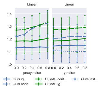
Figure 6: $\sqrt{\epsilon_{pehe}}$ on linear synthetic dataset. Error bar on 100 random models. We adjust one of $\alpha,\beta$ at a time. Results for ATE and post-treatment are similar.

We adjust the outcome and proxy noise level by $\alpha,\beta$ respectively. The output of $f$ is normalized by $C\coloneqq\mathrm{Var}_{\{\mathcal{D}|{\textnormal{t}}=t\}}(f({\textnormal{z}}))$. This means we need to use $0\leq\alpha<1$ to have a reasonable level of noise on ${\mathbf{y}}$ (the scales of mean and variance are comparable). Similar reasoning applies to ${\textnormal{z}}|{\mathbf{x}}$; outputs of $h,k$ have approximately the same range of values since the functions’ coefficients are generated by the same weight initializer.

As shown in Figure 6, our method again constantly outperforms CEVAE under linear outcome models. Interestingly, linear outcome models seem harder for both methods. While we did not dig into this point because this would be a digress from our purpose, we give two possible reasons: 1) under similar noise levels, the observed outcome values under nonlinear outcome models might be more informative about the values of z, because nonlinear models are often steeper than linear models for many values of z; 2) the two true linear outcome models for $t=0,1$ are more similar, particularly when the two potential outcomes are in small and similar ranges, and it is harder to distinguish and learning the two outcome models.

You can find more plots for latent recovery at the end of the paper.

E.2 IHDP

IHDP is based on an RCT where each data point represents a child with 25 features about their birth and mothers. Race is introduced as a confounder by artificially removing all treated children with nonwhite mothers. There are 747 subjects left in the dataset. The outcome is synthesized by taking the covariates (features excluding Race) as input, hence unconfoundedness holds given the covariates.

Following previous work, we split the dataset by 63:27:10 for training, validation, and testing.

E.3 Additional plots on synthetic datasets

See last pages.

Appendix F Discussions

Since our method works without the recovery of either hidden confounder or true score distribution, we often cannot see apparent relationships between recovered latent representation and the true hidden confounder/scores. It would be nice to directly see the learned representation preserves causal properties, for example, by some causally-specialized metrics, e.g. Suter et al. (2019).

Despite the formal requirement in Theorem 3.1 of fixed distribution of noise on ${\mathbf{y}}$, inherited from Khemakhem et al. (2020a), the experiments show evidence that our method can learn the outcome noise. We observed that, in most cases, allowing the noise distribution to be learned depending on ${\mathbf{z}},{\textnormal{t}}$ improves performance. Theoretical analysis of this phenomenon is an interesting direction for future work.

Also, our causal theory does not in principle require continuous latent distributions, though in Theorem 3.1, differentiability of ${\bm{f}}$ is inherited from iVAE. Given the fact that currently all nonlinear ICA based identifiability requires differentiable mapping between the latent and observables, directly based on it, theoretical extensions to discrete latent variable would be challenging. However, what is essential for CATE identification is the same transformation between true and recovered score distribution for both $t$, but the transformation needs not to be affine, and, possibly, neither injective. This opens directions for future extensions, based not necessarily on nonlinear ICA.

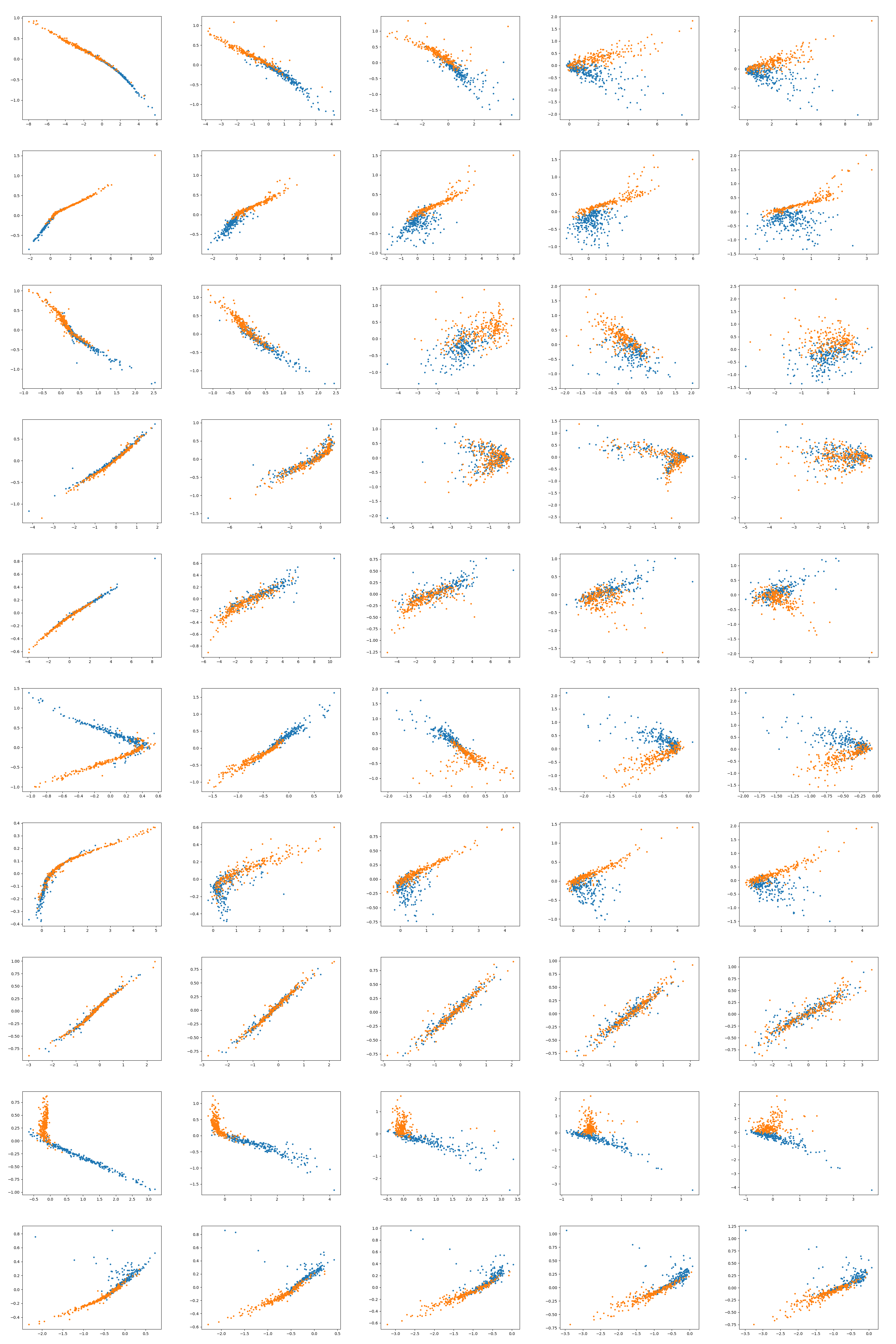
Figure 7: Plots of recovered-true latent under unobserved confounding. Rows: first 10 nonlinear random models, columns: proxy noise level.

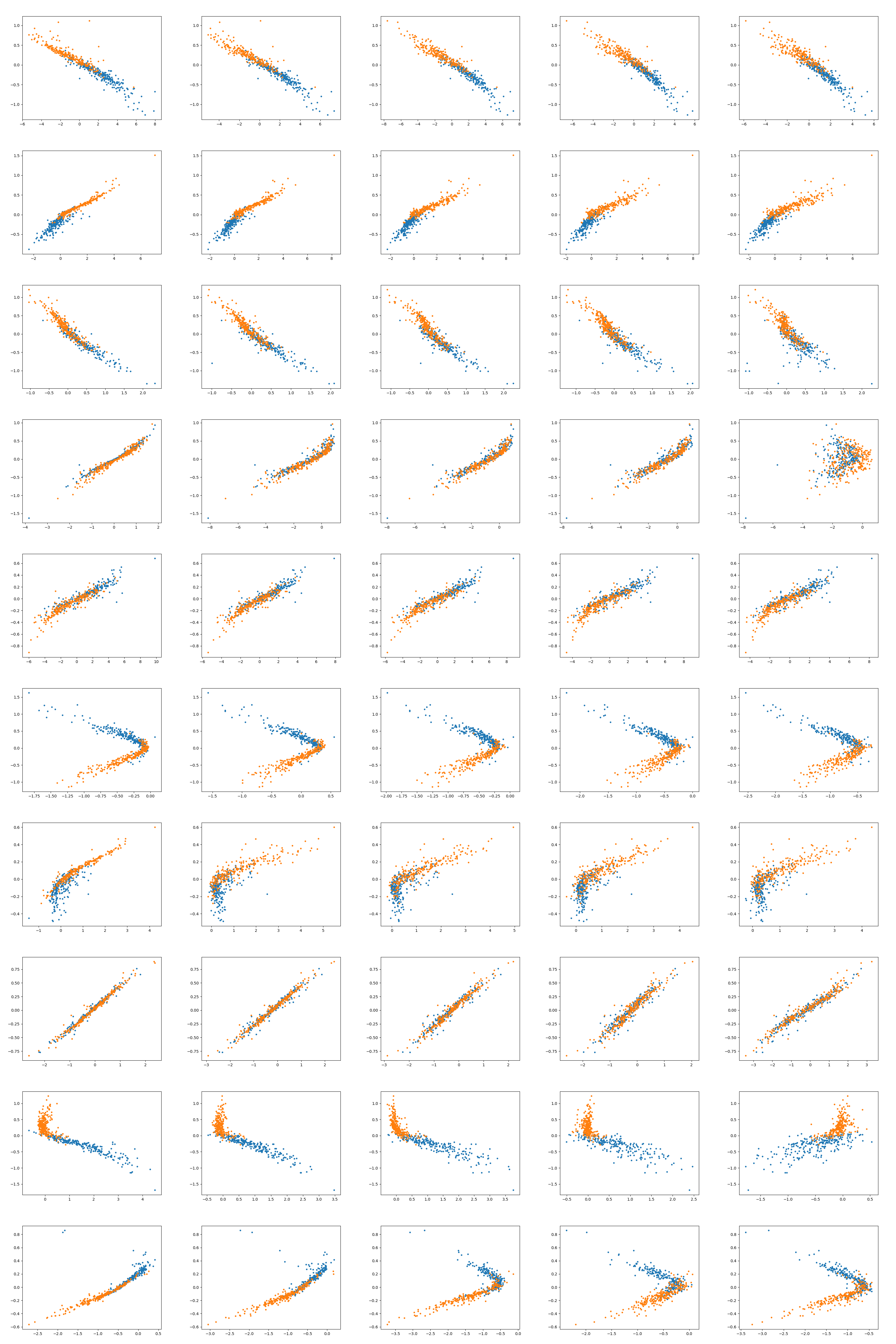
Figure 8: Plots of recovered-true latent under unobserved confounding. Rows: first 10 nonlinear random models, columns: outcome noise level.

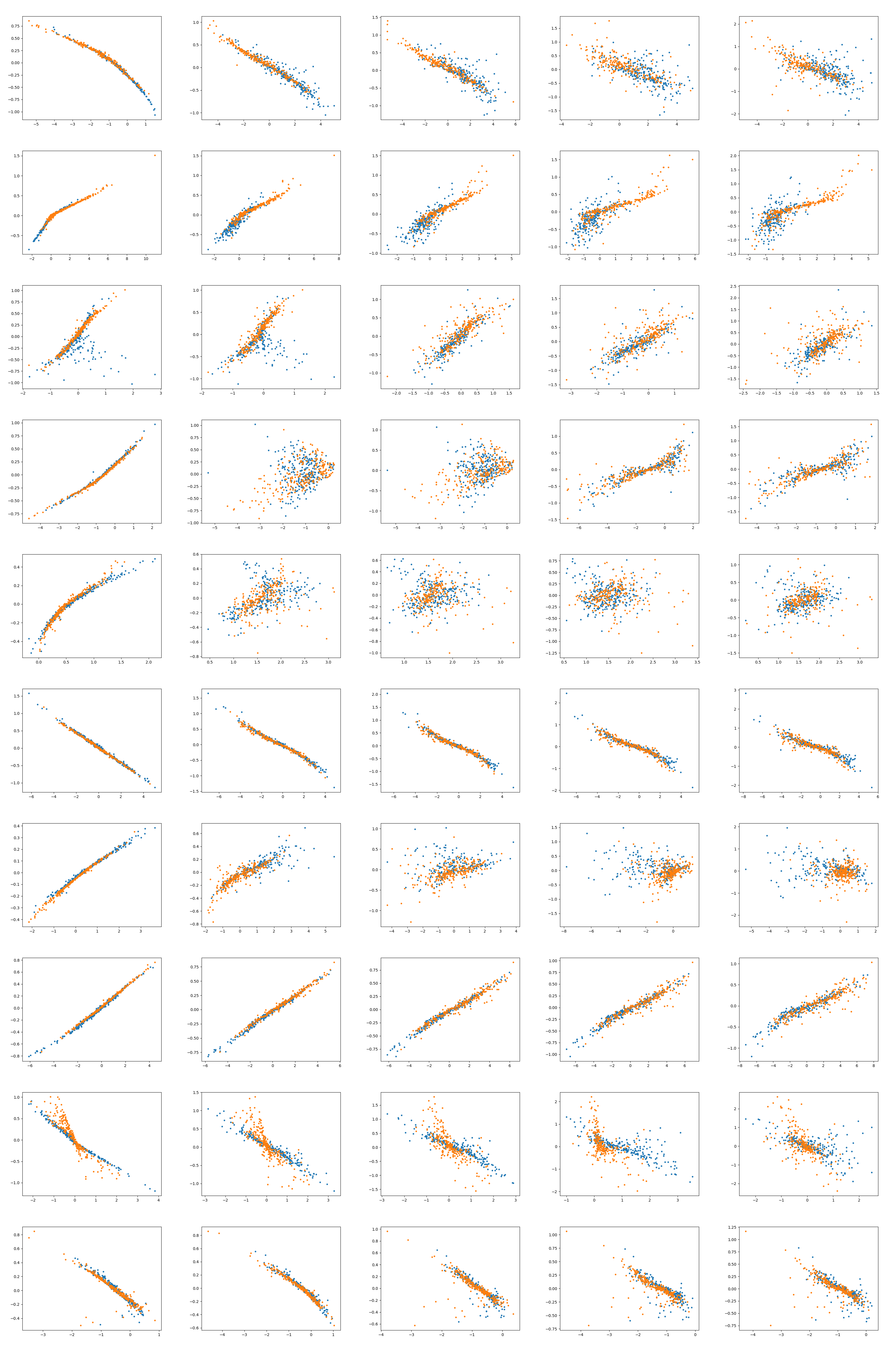
Figure 9: Plots of recovered-true latent when ignorability holds. Rows: first 10 nonlinear random models, columns: proxy noise level.

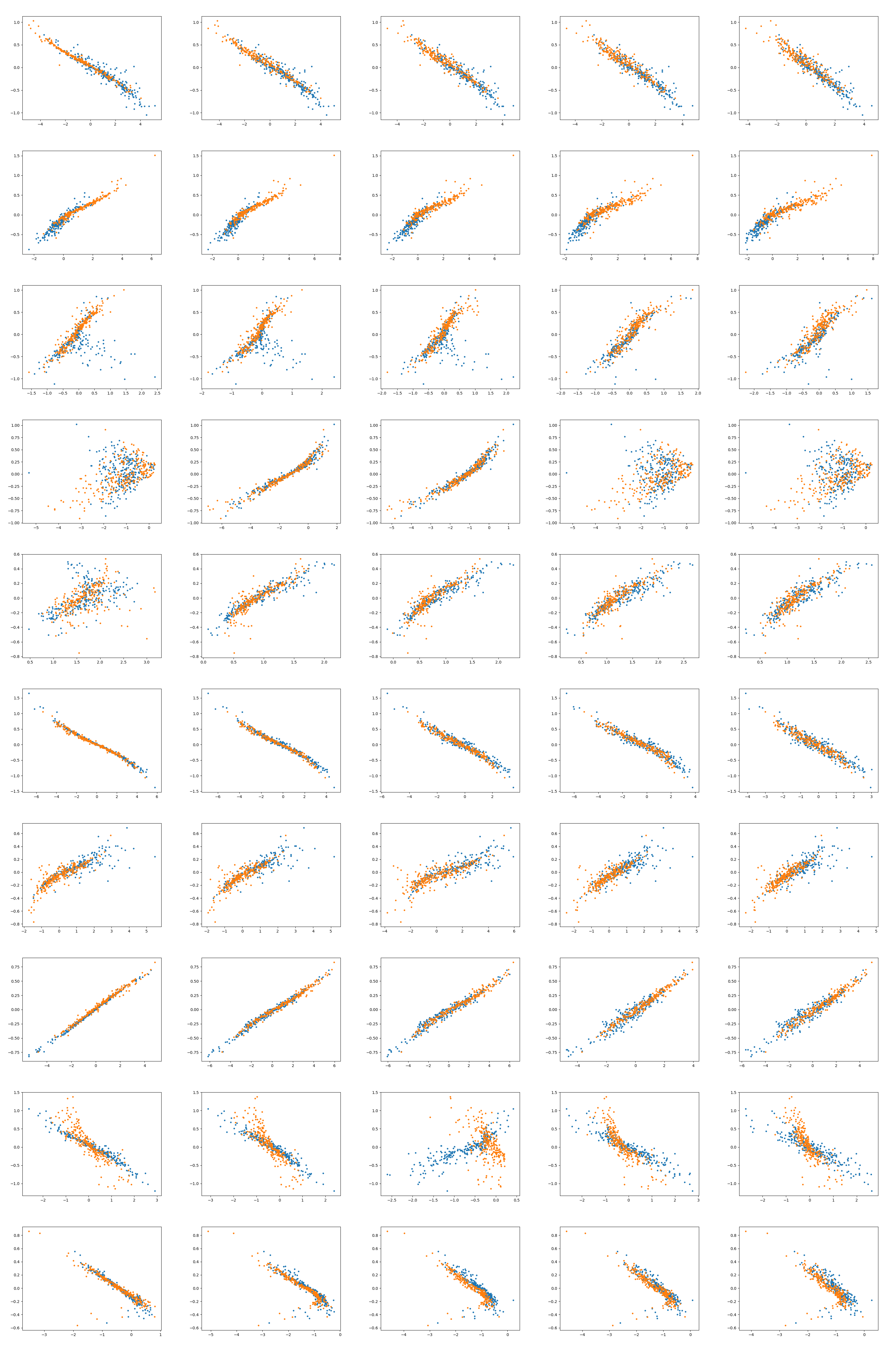
Figure 10: Plots of recovered-true latent when ignorability holds. Rows: first 10 nonlinear random models, columns: outcome noise level.

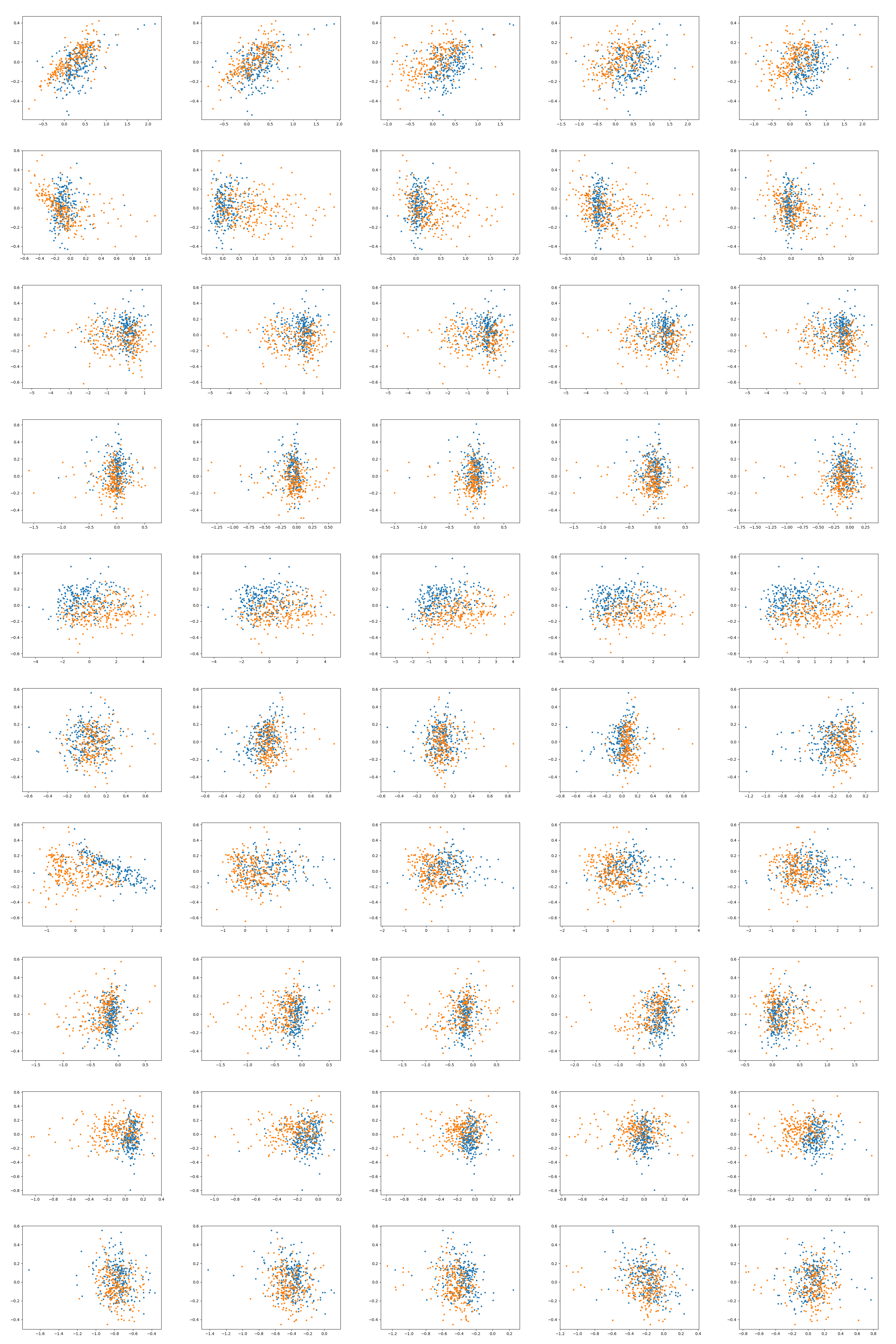
Figure 12: Plots of recovered-true latent on IVs. Rows: first 10 nonlinear random models, columns: outcome noise level.

References

- Abrevaya et al. (2015) Jason Abrevaya, Yu-Chin Hsu, and Robert P Lieli. Estimating conditional average treatment effects. Journal of Business & Economic Statistics, 33(4):485–505, 2015.
- Alaa and van der Schaar (2017) Ahmed M Alaa and Mihaela van der Schaar. Bayesian inference of individualized treatment effects using multi-task gaussian processes. In Advances in Neural Information Processing Systems, pages 3424–3432, 2017.
- Allman et al. (2009) Elizabeth S Allman, Catherine Matias, John A Rhodes, et al. Identifiability of parameters in latent structure models with many observed variables. The Annals of Statistics, 37(6A):3099–3132, 2009.
- Angrist et al. (1996) Joshua D Angrist, Guido W Imbens, and Donald B Rubin. Identification of causal effects using instrumental variables. Journal of the American statistical Association, 91(434):444–455, 1996.
- Anonymous (2020) Anonymous. Identifying treatment effects under unobserved confounding by causal representation learning. submitted to ICLR 2021, 2020.
- Anonymous (2021) Anonymous. beta-intact-vae: Identifying and estimating causal effects under limited overlap. arXiv preprint arXiv:2110.05225, 2021.
- Bonhomme and Weidner (2021) Stéphane Bonhomme and Martin Weidner. Posterior average effects. Journal of Business & Economic Statistics, (just-accepted):1–38, 2021.
- Chetverikov et al. (2018) Denis Chetverikov, Andres Santos, and Azeem M Shaikh. The econometrics of shape restrictions. Annual Review of Economics, 10:31–63, 2018.
- Cuturi (2013) Marco Cuturi. Sinkhorn distances: Lightspeed computation of optimal transport. In Advances in neural information processing systems, pages 2292–2300, 2013.
- Doersch (2016) Carl Doersch. Tutorial on variational autoencoders. arXiv preprint arXiv:1606.05908, 2016.
- D’Amour et al. (2020) Alexander D’Amour, Peng Ding, Avi Feller, Lihua Lei, and Jasjeet Sekhon. Overlap in observational studies with high-dimensional covariates. Journal of Econometrics, 2020.
- Gan and Li (2016) Li Gan and Qi Li. Efficiency of thin and thick markets. Journal of Econometrics, 192(1):40–54, 2016.
- Gopalan and Blei (2013) Prem K Gopalan and David M Blei. Efficient discovery of overlapping communities in massive networks. Proceedings of the National Academy of Sciences, 110(36):14534–14539, 2013.
- Greenland (1980) Sander Greenland. The effect of misclassification in the presence of covariates. American journal of epidemiology, 112(4):564–569, 1980.
- Hansen (2008) Ben B Hansen. The prognostic analogue of the propensity score. Biometrika, 95(2):481–488, 2008.
- Hartford et al. (2017) Jason Hartford, Greg Lewis, Kevin Leyton-Brown, and Matt Taddy. Deep iv: A flexible approach for counterfactual prediction. In International Conference on Machine Learning, pages 1414–1423, 2017.
- Hernan and Robins (2020) Miguel A. Hernan and James M. Robins. Causal Inference: What If. CRC Press, 1st edition, 2020. ISBN 978-1-4200-7616-5.
- Higgins et al. (2017) Irina Higgins, Loïc Matthey, Arka Pal, Christopher Burgess, Xavier Glorot, Matthew Botvinick, Shakir Mohamed, and Alexander Lerchner. beta-vae: Learning basic visual concepts with a constrained variational framework. In 5th International Conference on Learning Representations, 2017. URL https://openreview.net/forum?id=Sy2fzU9gl.
- Hill (2011) Jennifer L Hill. Bayesian nonparametric modeling for causal inference. Journal of Computational and Graphical Statistics, 20(1):217–240, 2011.
- Hyvärinen and Morioka (2016) Aapo Hyvärinen and Hiroshi Morioka. Unsupervised feature extraction by time-contrastive learning and nonlinear ICA. In Advances in Neural Information Processing Systems, pages 3765–3773, 2016.
- Hyvärinen et al. (2019) Aapo Hyvärinen, Hiroaki Sasaki, and Richard Turner. Nonlinear ica using auxiliary variables and generalized contrastive learning. In The 22nd International Conference on Artificial Intelligence and Statistics, pages 859–868, 2019.
- Imbens and Rubin (2015) Guido W Imbens and Donald B Rubin. Causal inference in statistics, social, and biomedical sciences. Cambridge University Press, 2015.
- Janzing and Scholkopf (2010) Dominik Janzing and Bernhard Scholkopf. Causal inference using the algorithmic markov condition. IEEE Transactions on Information Theory, 56(10):5168–5194, 2010.
- Jiang and Tanner (2008) Wenxin Jiang and Martin A Tanner. Gibbs posterior for variable selection in high-dimensional classification and data mining. The Annals of Statistics, 36(5):2207–2231, 2008.
- Johansson et al. (2016) Fredrik Johansson, Uri Shalit, and David Sontag. Learning representations for counterfactual inference. In International conference on machine learning, pages 3020–3029, 2016.
- Kallus et al. (2018) Nathan Kallus, Xiaojie Mao, and Madeleine Udell. Causal inference with noisy and missing covariates via matrix factorization. In Advances in neural information processing systems, pages 6921–6932, 2018.
- Kallus et al. (2019) Nathan Kallus, Xiaojie Mao, and Angela Zhou. Interval estimation of individual-level causal effects under unobserved confounding. In The 22nd International Conference on Artificial Intelligence and Statistics, pages 2281–2290, 2019.
- Kato (2013) Kengo Kato. Quasi-bayesian analysis of nonparametric instrumental variables models. The Annals of Statistics, 41(5):2359–2390, 2013.
- Khemakhem et al. (2020a) Ilyes Khemakhem, Diederik Kingma, Ricardo Monti, and Aapo Hyvarinen. Variational autoencoders and nonlinear ica: A unifying framework. In International Conference on Artificial Intelligence and Statistics, pages 2207–2217, 2020a.
- Khemakhem et al. (2020b) Ilyes Khemakhem, Ricardo Monti, Diederik Kingma, and Aapo Hyvarinen. Ice-beem: Identifiable conditional energy-based deep models based on nonlinear ica. Advances in Neural Information Processing Systems, 33, 2020b.
- Kim (2002) Jae-Young Kim. Limited information likelihood and bayesian analysis. Journal of Econometrics, 107(1-2):175–193, 2002.
- Kingma and Welling (2013) Diederik P Kingma and Max Welling. Auto-encoding variational bayes. arXiv preprint arXiv:1312.6114, 2013. URL http://arxiv.org/abs/1312.6114.
- Kingma et al. (2019) Diederik P Kingma, Max Welling, et al. An introduction to variational autoencoders. Foundations and Trends® in Machine Learning, 12(4):307–392, 2019.
- Kingma et al. (2014) Durk P Kingma, Shakir Mohamed, Danilo Jimenez Rezende, and Max Welling. Semi-supervised learning with deep generative models. In Advances in neural information processing systems, pages 3581–3589, 2014.
- Kipf and Welling (2017) Thomas N. Kipf and Max Welling. Semi-supervised classification with graph convolutional networks. In 5th International Conference on Learning Representations, 2017. URL https://openreview.net/forum?id=SJU4ayYgl.
- Kuroki and Pearl (2014) Manabu Kuroki and Judea Pearl. Measurement bias and effect restoration in causal inference. Biometrika, 101(2):423–437, 2014.
- Leskovec and Krevl (2014) Jure Leskovec and Andrej Krevl. Snap datasets: Stanford large network dataset collection, 2014.
- Liao and Jiang (2011) Yuan Liao and Wenxin Jiang. Posterior consistency of nonparametric conditional moment restricted models. The Annals of Statistics, 39(6):3003–3031, 2011.
- Louizos et al. (2017) Christos Louizos, Uri Shalit, Joris M Mooij, David Sontag, Richard Zemel, and Max Welling. Causal effect inference with deep latent-variable models. In Advances in Neural Information Processing Systems, pages 6446–6456, 2017.
- Lu et al. (2020) Danni Lu, Chenyang Tao, Junya Chen, Fan Li, Feng Guo, and Lawrence Carin. Reconsidering generative objectives for counterfactual reasoning. Advances in Neural Information Processing Systems, 33, 2020.
- Manski (2009) Charles F Manski. Identification for prediction and decision. Harvard University Press, 2009.
- Mastouri et al. (2021) Afsaneh Mastouri, Yuchen Zhu, Limor Gultchin, Anna Korba, Ricardo Silva, Matt J. Kusner, Arthur Gretton, and Krikamol Muandet. Proximal causal learning with kernels: Two-stage estimation and moment restriction. In ICML 2021: 38th International Conference on Machine Learning, pages 7512–7523, 2021.
- Matzkin (2007) Rosa L Matzkin. Nonparametric identification. Handbook of econometrics, 6:5307–5368, 2007.
- Miao et al. (2018) Wang Miao, Zhi Geng, and Eric J Tchetgen Tchetgen. Identifying causal effects with proxy variables of an unmeasured confounder. Biometrika, 105(4):987–993, 2018.
- Muandet et al. (2019) Krikamol Muandet, Arash Mehrjou, Si Kai Lee, and Anant Raj. Dual instrumental variable regression. arXiv preprint arXiv:1910.12358, 2019.
- Nagasawa (2021) Kenichi Nagasawa. Treatment effect estimation with noisy conditioning variables. arXiv preprint arXiv:1811.00667v3, 2021.
- Newey (1993) Whitney K Newey. Efficient estimation of models with conditional moment restrictions. 1993.
- Pearl (2009) Judea Pearl. Causality: models, reasoning and inference. Cambridge University Press, 2009.
- Puli and Ranganath (2020) Aahlad Puli and Rajesh Ranganath. General control functions for causal effect estimation from instrumental variables. Advances in neural information processing systems, 33:8440, 2020.
- Rissanen and Marttinen (2021) Severi Rissanen and Pekka Marttinen. A critical look at the identifiability of causal effects with deep latent variable models. NeurIPS 2021, to appear, 2021.
- Roeder et al. (2021) Geoffrey Roeder, Luke Metz, and Durk Kingma. On linear identifiability of learned representations. In International Conference on Machine Learning, pages 9030–9039. PMLR, 2021.
- Rosenbaum (2020) Paul R Rosenbaum. Modern algorithms for matching in observational studies. Annual Review of Statistics and Its Application, 7:143–176, 2020.
- Rosenbaum and Rubin (1983) Paul R Rosenbaum and Donald B Rubin. The central role of the propensity score in observational studies for causal effects. Biometrika, 70(1):41–55, 1983.
- Rubin (2005) Donald B Rubin. Causal inference using potential outcomes: Design, modeling, decisions. Journal of the American Statistical Association, 100(469):322–331, 2005.
- Schölkopf et al. (2021) Bernhard Schölkopf, Francesco Locatello, Stefan Bauer, Nan Rosemary Ke, Nal Kalchbrenner, Anirudh Goyal, and Yoshua Bengio. Toward causal representation learning. Proceedings of the IEEE, 2021.
- Schuler et al. (2020) Alejandro Schuler, David Walsh, Diana Hall, Jon Walsh, and Charles Fisher. Increasing the efficiency of randomized trial estimates via linear adjustment for a prognostic score. arXiv preprint arXiv:2012.09935, 2020.
- Shalit et al. (2017) Uri Shalit, Fredrik D Johansson, and David Sontag. Estimating individual treatment effect: generalization bounds and algorithms. In International Conference on Machine Learning, pages 3076–3085. PMLR, 2017.
- Shen et al. (2020) Xinwei Shen, Furui Liu, Hanze Dong, Qing Lian, Zhitang Chen, and Tong Zhang. Disentangled generative causal representation learning. arXiv preprint arXiv:2010.02637, 2020.
- Shi et al. (2019) Claudia Shi, David Blei, and Victor Veitch. Adapting neural networks for the estimation of treatment effects. In Advances in Neural Information Processing Systems, pages 2507–2517, 2019.
- Singh et al. (2019) Rahul Singh, Maneesh Sahani, and Arthur Gretton. Kernel instrumental variable regression. arXiv preprint arXiv:1906.00232, 2019.
- Sohn et al. (2015) Kihyuk Sohn, Honglak Lee, and Xinchen Yan. Learning structured output representation using deep conditional generative models. In Advances in neural information processing systems, pages 3483–3491, 2015.
- Sorrenson et al. (2019) Peter Sorrenson, Carsten Rother, and Ullrich Köthe. Disentanglement by nonlinear ica with general incompressible-flow networks (gin). In International Conference on Learning Representations, 2019.
- Srivastava et al. (2014) Nitish Srivastava, Geoffrey Hinton, Alex Krizhevsky, Ilya Sutskever, and Ruslan Salakhutdinov. Dropout: a simple way to prevent neural networks from overfitting. The journal of machine learning research, 15(1):1929–1958, 2014.
- Starling et al. (2019) Jennifer E Starling, Catherine E Aiken, Jared S Murray, Annettee Nakimuli, and James G Scott. Monotone function estimation in the presence of extreme data coarsening: Analysis of preeclampsia and birth weight in urban uganda. arXiv preprint arXiv:1912.06946, 2019.
- Stuart (2010) Elizabeth A. Stuart. Matching Methods for Causal Inference: A Review and a Look Forward. Statistical Science, 25(1):1 – 21, 2010. 10.1214/09-STS313. URL https://doi.org/10.1214/09-STS313.
- Suter et al. (2019) Raphael Suter, Djordje Miladinovic, Bernhard Schölkopf, and Stefan Bauer. Robustly disentangled causal mechanisms: Validating deep representations for interventional robustness. In International Conference on Machine Learning, pages 6056–6065. PMLR, 2019.
- Tarr and Imai (2021) Alexander Tarr and Kosuke Imai. Estimating average treatment effects with support vector machines. arXiv preprint arXiv:2102.11926, 2021.
- Tchetgen et al. (2020) Eric J Tchetgen Tchetgen, Andrew Ying, Yifan Cui, Xu Shi, and Wang Miao. An introduction to proximal causal learning. arXiv preprint arXiv:2009.10982, 2020.
- Tien (2021) Christian Tien. Instrumental common confounding. 2021. URL https://www.christiantien.com/publication/preprint/preprint.pdf.
- Van der Laan and Rose (2018) Mark J Van der Laan and Sherri Rose. Targeted learning in data science: causal inference for complex longitudinal studies. Springer, 2018.
- Veitch et al. (2019) Victor Veitch, Yixin Wang, and David Blei. Using embeddings to correct for unobserved confounding in networks. In Advances in Neural Information Processing Systems, pages 13792–13802, 2019.
- Vowels et al. (2020) Matthew James Vowels, Necati Cihan Camgoz, and Richard Bowden. Targeted vae: Structured inference and targeted learning for causal parameter estimation. arXiv preprint arXiv:2009.13472, 2020.
- Wager and Athey (2018) Stefan Wager and Susan Athey. Estimation and inference of heterogeneous treatment effects using random forests. Journal of the American Statistical Association, 113(523):1228–1242, 2018.
- Wang et al. (2020) Shanshan Wang, Liren Yang, Li Shang, Wenfang Yang, Cuifang Qi, Liyan Huang, Guilan Xie, Ruiqi Wang, and Mei Chun Chung. Changing trends of birth weight with maternal age: a cross-sectional study in xi’an city of northwestern china. BMC Pregnancy and Childbirth, 20(1):1–8, 2020.
- Wang and Blei (2019) Yixin Wang and David M Blei. The blessings of multiple causes. Journal of the American Statistical Association, 114(528):1574–1596, 2019.
- Wang et al. (2021) Ziyu Wang, Yuhao Zhou, Tongzheng Ren, and Jun Zhu. Scalable quasi-bayesian inference for instrumental variable regression. NeurIPS 2021, to appear, 2021.
- Wooldridge (2015) Jeffrey M Wooldridge. Control function methods in applied econometrics. Journal of Human Resources, 50(2):420–445, 2015.
- Wu and Fukumizu (2020) Pengzhou Wu and Kenji Fukumizu. Causal mosaic: Cause-effect inference via nonlinear ica and ensemble method. In International Conference on Artificial Intelligence and Statistics, pages 1157–1167. PMLR, 2020. URL http://proceedings.mlr.press/v108/wu20b.html.
- Yoon et al. (2018) Jinsung Yoon, James Jordon, and Mihaela van der Schaar. GANITE: Estimation of individualized treatment effects using generative adversarial nets. In International Conference on Learning Representations, 2018. URL https://openreview.net/forum?id=ByKWUeWA-.
- Zhang (2006) Tong Zhang. From epsilon-entropy to kl-entropy: Analysis of minimum information complexity density estimation. The Annals of Statistics, 34(5):2180–2210, 2006.
- Zhang et al. (2020) Weijia Zhang, Lin Liu, and Jiuyong Li. Treatment effect estimation with disentangled latent factors. arXiv preprint arXiv:2001.10652, 2020.