Topological changes due to non-equilibrium effects
by means of the statistical model of two-phase flow

Abstract

This paper presents the first results of the two-phase flow obtained using recently introduced physical, mathematical and numerical model of the intermittency region between two-phases (Wacławczyk 2017, 2021). The statistical interpretation of the intermittency region evolution equations allows to account for the non-equilibrium effects in the domain separating two phases. The source of non-equilibrium are spatial variations in the ratio of work done by volume and interfacial forces governing its width. As the statistical description of the two-phase flow differs from the deterministic two-phase flow models known in the literature, in the present work we focus discussion of the results on these differences. To this goal, the rising two dimensional gas bubble is studied; differences between equilibrium and non-equilibrium solutions are investigated. It is argued the statistical description of the intermittency region has potential to account for physical phenomena not considered previously in the computer simulations of two-phase flow.

1 Introduction

The main difference between single and multi-phase flow is in the topological changes of the boundaries separating coexisting phases and/or flow domain(s). The wide spectrum of physical phenomena at these boundaries governs the multi-phase flow and have to be accounted for in all multi-phase flow regimes. The numerical solution of the flow problems with moving boundary conditions is source of complexity of the numerical algorithms and has led to the development of the abundance of the computational techniques anderson1998 ; osher03 ; prosperetti06 ; trygg11 .

In fluid mechanics, the most popular approach splits the control volume containing neighboring phases with the sharp interface smooth enough to compute mean Gaussian curvature needed to determine capillary terms osher03 ; trygg11 . While the division of the given control volume is not arbitrary (as one would expect in the continuum mechanical model), the sharp interface model guarantees the highest possible numerical resolution of the interface (at worst in the single control volume and its nearest neighbors).

In the phase field methods, the control volume is divided by the diffusive interface anderson1998 . The main advantage of the phase field methods is in their physical interpretation based on theory of the Ginzburg-Landau free energy functional kim12 . However, the order parameter in the phase field model does not have clear physical interpretation. This is caused by the fact Allen-Cahn allen1979 and Cahn-Hilliard cahn1958 equations governing the phase field does not have a mathematical form of the classical transport equation. To overcome these difficulties and preserve conservation of the order parameter the Lagrange multiplayer techniques has been adopted kim12 ; kim14 .

In the fluid mechanics community it is assumed, that the numerical sharp and diffusive interface models follow the thermodynamic dividing plane model of Gibbs gibbs1874 and the smooth transition region model of van der Waals waals1979 . We note, that if this indeed is the case, they inherit the known shortcomings of these models, too. For instance, as the position of the Gibbs dividing plane $\mathbf{x}_{\Gamma}\,[m]$ is arbitrary lang15 ; faust2018 the (signed) distance measured from this position is not defined as well. In the phase field models it is often assumed the radius of the curvature $R\,[m]$ has to be much larger than the interface thickness $\epsilon_{h}\,[m]$. Otherwise a numerical robustness and physical interpretation of the phase field model(s) order parameter are impaired kim12 ; lang15 . As phase transitions (e.g. boiling) typically start at the molecular level from the mixture of fluid and its vapor (no bubble exists at this stage, yet) the assumption about $\epsilon_{h}/R\!\ll\!1$ ratio seems to restrict the range of the phase field model(s) application.

Whilst the mathematical and following physical imperfections of the aforementioned model equations can be compensated by a careful choice of the sophisticated numerical techniques (e.g. higher-order advection schemes liu1994 , the height function method cummins05 , adaptive mesh refinement popinet09 , Lagrange multiplayer kim14 , etc.) leading, eventually, to plethora of successful numerical predictions; the most striking flaw of the deterministic sharp/diffusive interface models seems to be their detachment from the experimental reality vrij1973 ; aarts2004 .

Moreover, one could also ask: how likely is it , that solution of the five cahn1958 ; allen1979 ; hirt81 ; osher1988 ; olsson05 , different (sets of) apparently unrelated partial differential equations, describing the same physical phenomenon(a), using different boundary conditions, leads to the same (or very similar) predictions?

The answers to some of these questions are given in twacl17 . Unlike described by the sharp and diffusive interface models the mesoscopic interface $\Gamma$ between two phases is rough and/or turbulent. It is disturbed by thermal fluctuations in the domain where particles of coexisting phases violently exchange energy dependent on the temperature and cohesive forces of the given system. For this reason, the width of this domain is estimated to be $\epsilon_{h}\!\sim\!\sqrt{k_{B}T/\sigma}\!>\!0$ where $k_{B}\,[J/K]$ is the Boltzman constant, $T\,[K]$ is the absolute temperature and $\sigma\,[J/m^{2}]$ is the surface tension coefficient vrij1973 ; aarts2004 . The discrepancy between true nature of the interface and its smooth, deterministic models has led the present author to development of the description that is alternative for the sharp and diffusive interface models and yet it shows they can be considered as complementary components of the same statistical description twacl15 ; twacl17 ; twacl21 .

In the present work, recently derived twacl15 equation describing evolution of the intermittency region is coupled with the Navier-Stokes incompressible flow solver and used to simulate flow of the rising, two-dimensional gas bubble. In addition, we use non-equilibrium solution of the modified Ginzburg-Landau functional twacl17 ; twacl21 derived by the present author to introduce the new mechanism of the topological changes in two-phase flow. To this goal, the two cases are considered: first, when characteristic length scale field $\epsilon_{h}\left(\mathbf{x},t\right)$ governing the local intermittency region width is constant, and second, when $\epsilon_{h}\left(\mathbf{x},t\right)$ is given by the prescribed analytical function.

This paper is organized as follows. In the next section, derivation of the intermittency region evolution equation and its relation with the modified Ginzburg-Landau free energy functional is recalled twacl17 ; twacl21 . Next, we present the numerical method and set-up of the two-dimensional numerical experiment. Finally, obtained results are discussed in context of difference between equilibrium and non-equilibrium effects in two-phase flows and differences between the predictions of the deterministic and the statistical intermittency region models.

2 Statistical model of the intermittency region

In this section we briefly recall arguments already presented in works twacl15 ; twacl17 ; twacl21 . Therein the derivation, physical interpretation and convergence of numerical solution of the intermittency region evolution equation is investigated. The new contribution in these work is description of the intermitency region in terms of probability of finding the mesoscopic sharp interface $\Gamma$. Moreover, establishing its relation to the minimization procedure of the modified Ginzburg-Landau free energy functional.

2.1 Derivation of the cumulative distribution function transport equation

We assume, the interface between two-phases is domain named the microscopic intermittency region. Therein, the position of the sharp interface $\Gamma$ (herein defined on the molecular level) can be found with the non-zero probability described by the cumulative distribution function $\alpha\,[-]$. It is important to note, the intermittency region paradigm was first introduced and developed for modeling of turbulence interface interactions brocchini01a ; mwaclawczyk11 ; waclawczyk2015 . In twacl17 we have drew analogy between the interface interacting with turbulence and sharp interface $\Gamma$ agitated by thermal fluctuations. In both cases, these phenomena can be described as stochastic processes. This allowed us to use the conditional averaging procedure pope88 and eddy viscosity model waclawczyk2015 to close unknown correlations as in turbulence-interface interaction model. As a result, equation for evolution of the probability of finding the mesoscopic sharp interface $\Gamma$: $\alpha\,[-]$, is derived

$$\frac{\partial\alpha}{\partial t}\!+\!\mathbf{w}\nabla\alpha\!=\!\nabla\cdot\left(D\nabla\alpha\right)-|\langle\mathbf{n}_{\Gamma}\rangle_{\Gamma}|\nabla{\left(D\Sigma\right)}\!\cdot\!\mathbf{n}_{\gamma}$$ (1)

where $\mathbf{w}\,[m/s]$ is velocity of the regularized interface $\gamma$ defined by the expected position of $\Gamma$: $\alpha\left(\psi\!=\!0\right)\!=\!1/2$ , $\mathbf{n}_{\gamma}$ is vector normal to $\gamma$, $\mathbf{n}_{\Gamma}$ is vector normal to $\Gamma$, $\langle\cdot\rangle_{\Gamma}$ is the conditional average operator and $D\!=\!C\left(\mathbf{x},t\right)\epsilon_{h}\left(\mathbf{x},t\right)\,[m^{2}/s]$ is the diffusivity coefficient. $C\left(\mathbf{x},t\right)$, $\epsilon_{h}\left(\mathbf{x},t\right)$ are velocity and length scales characterizing the intermittency region, respectively. The first RHS term in Eq. (1) is responsible for spreading of the intermittency region width, the second one has been shown to be the counter gradient diffusion responsible for its contraction mwaclawczyk11 ; waclawczyk2015 .

As Eq. (1) contains an unclosed RHS term with the unknown surface density $\Sigma\,[m^{2}/m^{3}]$, we have used results in cahn1958 ; olsson05 ; chiu11 for its conservative closure and its physical interpretation twacl21 . Hence, $\alpha\,[-]$ evolution equation reads

$$\frac{\partial\alpha}{\partial t}\!+\!\nabla\!\cdot\!\left(\mathbf{w}\alpha\right)\!=\!\nabla\cdot\left[D|\nabla\alpha|\mathbf{n}_{\gamma}\!-\!C\alpha\left(1-\alpha\right)\mathbf{n}_{\gamma}\right].$$ (2)

The coefficients $C\,[m/s],\,D\,[m^{2}/s]$ in Eq. (2) specify the characteristic length $\epsilon_{h}\!\sim\!D/C\,[m]$ and time $\tau_{h}\!\sim\!D/C^{2}\,[s]$ scales governing its solution and in general can be functions of space and time. Thus, in works kmtw14 ; twaclawczyketal14 ; waclawczyk2015 it was shown Eq. (2) can be used to predict the intermittency region evolution due to interaction of turbulent eddies with the macroscopic interface $\gamma$ (the same interface as in the standard volume of fluid (VOF) and level-set (SLS) numerical models).

The steady state solution of Eq. (2) with $\epsilon_{h}\!=\!const.$ and $\mathbf{w}\!=\!\mathbf{u}\!=\!0$ is given by the regularized Heaviside function

$$\alpha\left(\psi\right)=\frac{1}{1+\exp{\left(-\psi\left(\mathbf{x},t\right)/\epsilon_{h}\right)}}=\frac{1}{2}\left[1+\tanh{\left(\frac{\psi\left(\mathbf{x},t\right)}{2\epsilon_{h}}\right)}\right]$$ (3)

and its inverse function that is the signed distance from the expected position of the regularized interface $\gamma$ defined by the level-set $\psi\left(\alpha\!=\!1/2\right)\!=\!0$

$$\psi\left(\alpha\right)=\epsilon_{h}\ln{\left[\frac{\alpha\left(\psi\right)}{1-\alpha\left(\psi\right)}\right]}.$$ (4)

As noticed by the present author twacl15 , Eqs. (3) and (4) are known to characterize the cumulative distribution $\alpha\left(\psi\right)$, and quantile $\psi\left(\alpha\right)$ functions of the logistic distribution. Additionally, the gradient of $\alpha\left(\psi\right)$ given by the formula

$$\nabla\alpha=\frac{\tilde{\delta}\left(\alpha\right)}{\epsilon_{h}}\nabla\psi,$$ (5)

where $\tilde{\delta}\left(\alpha\right)/\epsilon_{h}\!=\!\alpha\left(1\!-\!\alpha\right)/\epsilon_{h}$ is the probability density function of the logistic distribution. Computation of $\nabla\alpha\,[1/m]$ with Eq. (5) bridges the numerical problems with approximation of steep functions gradients (see $\alpha$ when $\epsilon_{h}\rightarrow 0$ and analysis in twacl15 ). Eq. (5) can also be interpreted as calculation of $\nabla\alpha$ in the $\mathbf{n}_{\gamma}$ direction

$$\nabla\alpha\cdot\mathbf{n}_{\gamma}\!=\!\frac{\partial\alpha}{\partial\psi}\!=\!\frac{\tilde{\delta}\left(\alpha\right)}{\epsilon_{h}}.$$ (6)

This observation was recently used in holger2021 to reformulate the modified Ginzburg-Landau free energy functional for its solution in the local coordinate system normal in every point to the interface $\gamma$. While Eq. (6) is exact, the Laplacian $\nabla\!\cdot\!\left\{\nabla\left[\alpha\left(\psi\right)\!\cdot\!\mathbf{n}_{\gamma}\right]\right\}$ in the normal direction can be only approximated in similar way when the interface curvature $\kappa\!\ll\!1$.

Curiously, the definition of the chemical potential and the corresponding modified Ginzburg-Landau functional in twacl17 and holger2021 is the same (to details in the coefficients and the fact that different solution norms are used mirja20 ). The advantage of description used herein over the classical phase field models is sound physical interpretation of the order parameter $\alpha\,[-]$, its gradient $\nabla\alpha\,[1/m]$ and the order parameter inverse function $\psi\,[m]$, see Eqs. (3,5,4) respectively.

This makes the difference as for instance, one can use the physical meaning of the cumulative distribution function given by Eq. (3) to pinpoint the position of the Gibbs dividing surface $\mathbf{x}_{\Gamma}$. The Gibbs dividing surface can be defined as the expected position of the sharp interface $\Gamma$ agitated by the stochastic thermal fluctuations. This position is given by the level-sets $\alpha\left(\psi\!=\!0\right)\!=\!1/2$ and describes the two dimensional smooth surface that is called the sharp interface in the deterministic models of the intermittency region.

In twacl15 it was noticed that substitution of Eq. (5) into Eq. (2) results in

$$\frac{\partial\alpha}{\partial t}+\mathbf{w}\nabla\alpha=\nabla\cdot\left[C\tilde{\delta}\left(\alpha\right)\left(|\nabla\psi|-1\right)\mathbf{n}_{\gamma}\right],$$ (7)

where $\mathbf{n}_{\gamma}\!=\!\nabla\alpha/|\nabla\alpha|\!=\!\nabla\psi/|\nabla\psi|$. In the present work we separate the advection and re-initialization steps in Eq. (7), which leads to

$$\frac{\partial\alpha}{\partial t}\!+\!\mathbf{w}\nabla\alpha\!=\!\frac{\partial\alpha}{\partial t}\!+\!\frac{\tilde{\delta}\left(\alpha\right)}{\epsilon_{h}}\mathbf{w}\!\cdot\!\nabla\psi\!=\!0,$$ (8)

$$\frac{\partial\alpha}{\partial\tau}\!=\!\nabla\!\cdot\!\left[C\tilde{\delta}\left(\alpha\right)\left(\left|\nabla\psi\right|\!-\!1\right)\mathbf{n}_{\gamma}\right],$$ (9)

where $\tau\,[s]$ is time needed to obtain the equilibrium solution of Eq. (9). In our works, this form of Eq. (2) is preferred for numerical solution and theoretical analysis.

At first, the choice of the partial differential algebraic equation (4-7) for the model of two-phase flow in fluid mechanics appears to be surprising. However, it is known ascher1998 , the equations of this type describe systems with the large separation of scales (e.g. chemical kinetics in quasi steady state and partial equilibrium approximations, molecular dynamics, optimal control etc.). This suits our goal of derivation of the intermittency region model that is closer to experimental reality than known in the literature thermodynamic descriptions of the interface between two-phases.

2.2 Re-initialization as minimization of the modified Ginzburg-Landau functional

In twacl21 it was shown, when the characteristic length $\epsilon_{h}\,[m]$ and velocity $C\,[m/s]$ scales governing evolution of the intermittency region are constant, this region is remaining in the equilibrium state according to the modified Ginzburg-Landau functional describing interfacial energy of the intermittency region twacl17 . In this case, the solution of Eq. (9) in the Conservative Level-Set method (CLS) olsson05 is called re-initialization of the function $\alpha$. In this numerical method, the re-initialization step is used to restore deformed due to numerical errors in the advection step function $\alpha$ to its original form given by Eq. (3).

In the limit $\epsilon_{h}\!\rightarrow\!0$, Eqs. (5) and (9) can be used to derive the re-initialization equation of the signed-distance function $\psi$ used in the Standard Level-Set (SLS) method twacl15 ; twacl17 . Here, the goal of the re-initialization step is similar. The goal function in reconstruction procedure is $\psi\,[m]$ disturbed by the numerical errors introduced during the advection step osher03 . Eqs. (4) and (7) explain that these two functions (and two models of the intermittency region) are closely related. Moreover, the present author has proven twacl17 , the re-initialization procedure in the SLS osher03 and CLS olsson05 level-set methods are equivalent to minimization of the free energy functional containing the term which accounts for the regularized interface $\gamma$ deformation.

We note that before work twacl17 the presence of term with $\nabla\alpha$ and the interface curvature $\kappa$ in the definition of chemical potential was postulated folch1999 . Extension of the original free energy Ginzburg-Landau functional by the additional term containing the interface curvature was also proposed in jamet2008 . However, as noticed in mirja20 the derivations in folch1999 ; jamet2008 and twacl15 ; twacl17 were carried out in the different norms. Moreover, as described in Section 1 the present work is driven by the attempt to paint more physical and general picture of the interface. In particular when it is agitated by the thermal or turbulent fluctuations, whereas the works folch1999 ; jamet2008 use mainly mathematical arguments.

2.3 Non-equilibrium of energy ratio in intermittency region

In most of the analytical and numerical discussions presented in the literature it is assumed, the interface or intermittency region are passive actors advected by the fluid velocity. In our view, the role of intermittency region in the multi-phase flow is much more complex. The intermittency region is open system that can interplay with neighboring phases through exchange of the mass and/or energy. In particular, in the case of phase changes it mediates in the exchange of mass and energy. For these reasons, the intermittency region between two weakly miscible phases may not be in the equilibrium state as it is typically assumed in the known sharp and diffusive interface models. Next it is demonstrated, that local non-equilibrium effects can influence distribution of the material properties of the phases, and hence, affect the two-phase flow scenario.

Driven by this general picture in the recent work twacl21 the non-equilibrium solution of Eqs. (7) and (8) was introduced. Therein we have shown, that statistical model of the intermittency region can also be extended to the case when $\epsilon_{h}\left(\mathbf{x},t\right)\!\neq\!const.$. In particular we have derived the free energy functional with $\nabla\alpha\!\cdot\!\nabla\epsilon_{h}$ term showing the variation of volume and interfacial forces work ratio should affect the cumulative distribution function $\alpha\left(\psi\right)$ shape. Moreover, we have demonstrated the stationary solution of Eq. (9) can be used as approximate solution of the non-equilibrium problem when used in a spirit of re-initialization as in the CLS and SLS numerical methods.

In what follows we repeat derivation of the approximate solution already presented in twacl21 . For mathematical details regarding the modified Ginzburg-Landau free energy functional the interested reader should refer to twacl21 .

The equilibrium condition obtained from the stationary solution to Eq. (9) reads

$$\nabla\alpha\!=\!|\nabla\alpha|\mathbf{n}_{\gamma}\!=\!\frac{\alpha\left(1\!-\!\alpha\right)}{\epsilon_{h}\left(\mathbf{x},t\right)}\mathbf{n}_{\gamma}.$$ (10)

Eq. (10) is formulated in the direction $\mathbf{n}_{\gamma}$ normal to the regularized interface $\gamma$, hence, it may be rewritten as

$$\frac{\partial\alpha}{\partial\psi}\left|\frac{\partial\psi}{\partial\mathbf{x}}\right|\!=\!\frac{1}{\epsilon_{h}\left(\mathbf{x},t\right)}\alpha\left(1\!-\!\alpha\right),$$ (11)

where it is assumed $\partial\alpha/\partial\psi\!>\!0$ meaning $\alpha\left(\psi\right)$ is expected to be the cumulative distribution function with infinite support analogously to Eq. (5). Next, we assume $|\nabla\psi|\!\equiv\!1$ in Eqs. (10) and (11). As a result, substitution of Eq. (10) into Eq. (2) with $D\left(\mathbf{x},t\right)\!=\!C\epsilon_{h}\left(\mathbf{x},t\right)$ let us derive Eq. (7) with the variable characteristic length scale governing width of the intermittency region. The assumption $|\nabla\psi|\!\equiv\!1$ means the signed distance function $\psi\left(\mathbf{x},t\right)$ spans the space where surface averaged oscillations of the sharp interface $\Gamma$ take place. On average, these oscillations occur only in the direction $\mathbf{n}_{\gamma}$ normal to the expected position $\psi\!=\!0$ of the regularized interface $\gamma$.

Further, it is noticed at each point $\left(\mathbf{x},t\right)$ of the field $\epsilon_{h}\left(\mathbf{x},t\right)$ the signed distance function $\psi\left(\mathbf{x},t\right)$ is given. Hence, the knowledge of the field $\psi\left(\mathbf{x},t\right)$ gives $\left(\mathbf{x},t\right)$ and thus $\epsilon_{h}\left(\mathbf{x},t\right)$. Therefore, we introduce $\epsilon_{h}^{\psi}\left(\mathbf{x},t\right)$ denoting $\epsilon_{h}\left(\mathbf{x},t\right)$ determined using $\psi\left(\mathbf{x},t\right)$. This let us to integrate Eq. (11) in the local coordinate system attached to the regularized interface $\gamma$. As $\gamma$ is defined by $\psi\left(\mathbf{x},t\right)\!=\!0$, $\psi\left(\mathbf{x},t\right)$ is the normal coordinate with the origin at $\psi\left(\mathbf{x},t\right)\!=\!0$ of this local system. At each fixed point of given $\alpha\left(\psi\right),\,\psi\left(\alpha\right),\,\epsilon_{h}\left(\mathbf{x},t\right)$ fields this integration reads

$$\int^{1/2}_{\alpha\left(\psi\right)}\frac{d\alpha^{\prime}}{\alpha^{\prime}\left(1\!-\!\alpha^{\prime}\right)}=\int^{0}_{\psi\left(\alpha\right)}\frac{d\psi^{\prime}}{\epsilon_{h}^{\psi^{\prime}}\!\left(\mathbf{x},t\right)}.$$ (12)

The integration (12) is performed from the arbitrary point located at the signed-distance from the regularized interface $\alpha\left(\psi\right)\!-\!\psi\left(\alpha\right)$ to the expected position of the regularized interface $\psi\left(\alpha\!=\!1/2\right)\!=\!0$. One notes the LHS integration in Eq. (12) does not assume or result in any specific form/shape of the function $\alpha\left(\psi\right)$.

To reconstruct the equilibrium solution when $\epsilon_{h}\left(\mathbf{x},t\right)\!=\!const.$ it is necessary to preserve the mapping between $\alpha\left(\psi\right)\!-\!\psi\left(\alpha\right)$, see Eq. (4). For this reason, it is more convenient to reformulate the RHS integral in Eq. (12) using a variable substitution as follows

$$\int^{0}_{\psi\left(\alpha\right)}\frac{d\psi^{\prime}}{\epsilon_{h}^{\psi^{\prime}}\!\left(\mathbf{x},t\right)}\!=\!\psi\left(\alpha\right)\int^{0}_{1}\frac{dt^{\prime}}{\epsilon_{h}^{t^{\prime}\psi}\!\left(\mathbf{x},t\right)}\!=\!\psi\left(\alpha\right)\mathcal{I\left(\psi\right)}$$ (13)

where $t^{\prime}\!\in\![0,1]$ is the parameter such that $\psi^{\prime}\!=\!t^{\prime}\psi$ and $d\psi^{\prime}\!=\!dt^{\prime}\psi$, furthermore $\mathcal{I\left(\psi\right)}$ is used to denote the integral on the RHS of Eq. (13).

After integration of Eq. (11) with Eq. (13) one obtains

$$\psi\left(\alpha\right)=\frac{1}{\mathcal{I\left(\psi\right)}}ln\left[\frac{\alpha\left(\psi\right)}{1-\alpha\left(\psi\right)}\right].$$ (14)

It is noted, Eq. (14) can be the source of numerical problems when $\alpha\rightarrow 0$ or $\alpha\rightarrow 1$. In these limits, due to the finite computer arithmetic computation of the natural logarithm is ill conditioned (see discussion of this problem in twacl15 ) and some measures must be taken to account for it. In the code, it is chosen to solve Eq. (9) only in the region where the numerical solution is still possible assuming: $|\nabla\psi|\!=\!1$ and hence $\partial\alpha/\partial\tau\!=\!0$, outside.

At the given, arbitrary point $\left(\mathbf{x},t\right)$, the signed distance $\psi\left(\mathbf{x},t\right)$ has the known value. For this reason, at the point $(\mathbf{x},t)$ the integral $\mathcal{I\left(\psi\right)}\!=\!const.$ and thus the inverse relation is also true

$$\alpha\left(\psi\right)\!=\!\frac{1}{1+\exp{\left[-\psi\left(\alpha\right)\mathcal{I\left(\psi\right)}\right]}}.$$ (15)

In the present work, Eq. (15) is called the approximate, semi-analytical solution of Eq. (9).

When the field $\epsilon_{h}\left(\mathbf{x},t\right)\!=\!const.$, Eq. (12) and Eq. (13) reduce to the equilibrium solution, which is guaranteed by the definition of $\mathcal{I\left(\psi\right)}$. Thus, the mapping given by Eq. (14) or the form of $\alpha\left(\psi\right)$ given by Eq. (15) can be employed during numerical solution of the system given by Eqs. (8) and (9) to model how the $\epsilon_{h}\left(\mathbf{x},t\right)$ field is affecting changes of the cumulative distribution function $0\!<\!\alpha\left(\psi\right)\!<\!1$ profile.

In what follows, we will couple described above approximate solution of Eq. (9) given by Eq. (15) with the Navier-Stokes equation solver to predict how non-equilibrium affects affect the flow of the two-dimensional rising gas bubble.

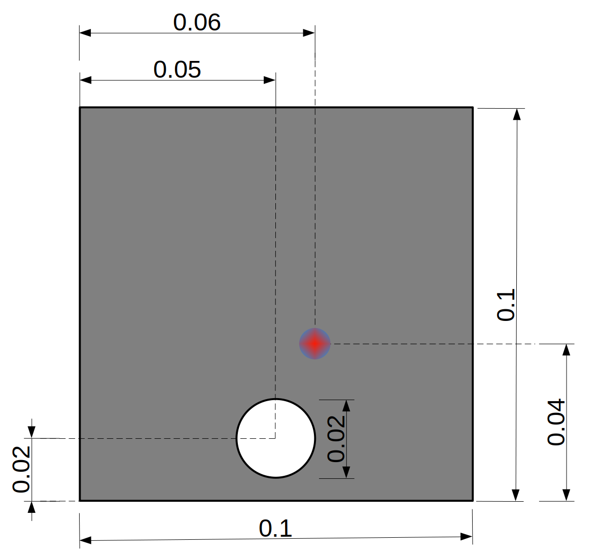
Figure 1: The schematic sketch of the flow case, all dimensions are in meters. The colored spot shows fixed position of variation in the characteristic length scale field $\epsilon_{h}\left(\mathbf{x},t\right)$ given by Eq. (19).

3 Numerical method

This section describes the numerical method used in the present paper for coupling of Eqs. (8, 9, 15) with the incompressible Navier-Stokes solver. In addition, details of incorporation of the non-equilibrium effects into the two-phase flow solver are described.

3.1 Flow solver and one-fluid model implementation

In the present paper, the second-order accurate finite volume flow solver in the collocated variable arrangement is used schaefer06 ; peric02 . For detailed description of the algorithm(s) and presentation of the results, see previous works by the present author waclawczyk05 ; waclawczyk06 ; waclawczyk07 ; waclawczyk08 ; waclawczyk08_2 ; waclawczyk08_3 ; waclawczyk08_phd ; waclawczyk2015 . As in these references, herein, the incompressible Navier-Stokes equation in the conservative form is solved. The momentum conservation equation is coupled with the Poisson equation to bind pressure and velocity fields in the SIMPLE procedure. The equilibrium between the pressure gradient and mass forces is established using the same numerical operators for their discretization zun07 . In this standard solver of incompressible flow, the two-phase flow model using the one-fluid formulation trygg11 is implemented; in the present work the presence of the capillary forces is neglected. Material properties of one-fluid change according to relations

$$\rho=\rho_{1}\alpha+\rho_{2}\left(1-\alpha\right),$$ (16)

$$\mu=\mu_{1}\alpha+\mu_{2}\left(1-\alpha\right),$$ (17)

where $\rho\,[kg/m^{3}],\,\mu\,[Pa\!\cdot\!s]$ denote density and dynamic viscosity of the mixture of two phases; $\rho_{k},\,\mu_{k},\,\,k=1,2$ are density and dynamic viscosity of pure fluid and gas phases, respectively.

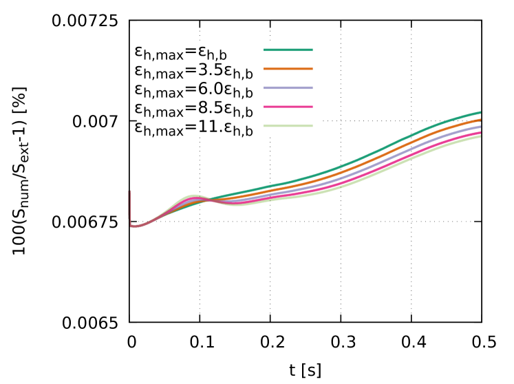
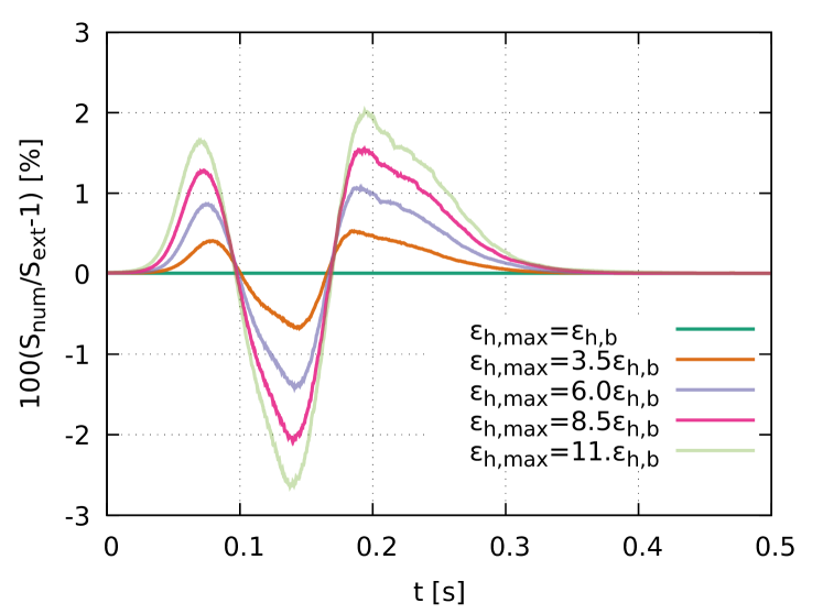
Figure 2: The mass conservation of gas during coupled simulations with constant $\epsilon_{h}\left(\mathbf{x},t\right)\!=\!\epsilon_{h,b}$ and variable characteristic length scale field $\epsilon_{h}\left(\mathbf{x},t\right)$. Total mass is computed using the c.d.f-s $\alpha\left(\psi\right)$ (left) and $\alpha_{d}\!\left(\psi\right)$(right). $\epsilon_{h,max}$ denotes the maximum magnitude of $\epsilon_{h}\left(\mathbf{x},t\right)$ given by Eq. (12).

The advection Eq. (8) is discretized in time using the second-order accurate implicit Euler method. For discretization of the convective term in space, the deferred-correction method with the second-order accurate TVD MUSCL flux limiter xue98 is employed. The same temporal and spatial discretization is used for velocity components in the Navier-Stokes equation. Re-initialization equation (9) is integrated in time using the explicit third-order accurate TVD Runge-Kutta method gottlieb98 . The constrained interpolation twacl17 ; twacl21 is used to discretize $\tilde{\delta}\left(\alpha\right)\!=\!\alpha\left(1-\alpha\right)$, in Eq. (9). For more details about numerical schemes and discretization used to solve Eqs. (8) and (9), refer to Appendixes in twacl15 ; twacl17 ; twacl21 .

It is noticed, Eq. (7) in the limit $\epsilon_{h}\rightarrow 0$ guarantees the statistical model of the intermittency region will converge to the solution obtained using the sharp interface model(s). We choose base or minimal width of the intermittency region as $\epsilon_{h,b}\!=\!\sqrt{2}\Delta x/4$; in twacl15 it was checked this selection guarantees the second order convergence of Eq. (9) and its higher-order derivatives.

Furthermore it is noted, in the statistical model of the intermittency region, unlike in some phase field solvers kim12 , there is no danger the material properties of the fluids will have nonphysical values. This is due to the fact that $\alpha\left(\psi\right)$ is the cumulative distribution function (see Eq. (3)) and it is incorporated into the solution procedure. Therefore, from its definition it is always bounded $0\!<\!\alpha\left(\psi\right)\!<\!1$.

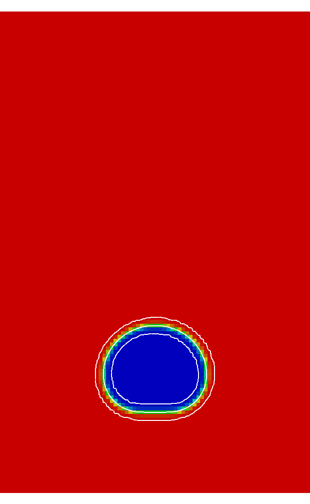
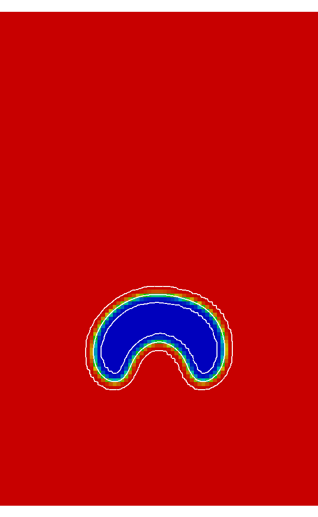
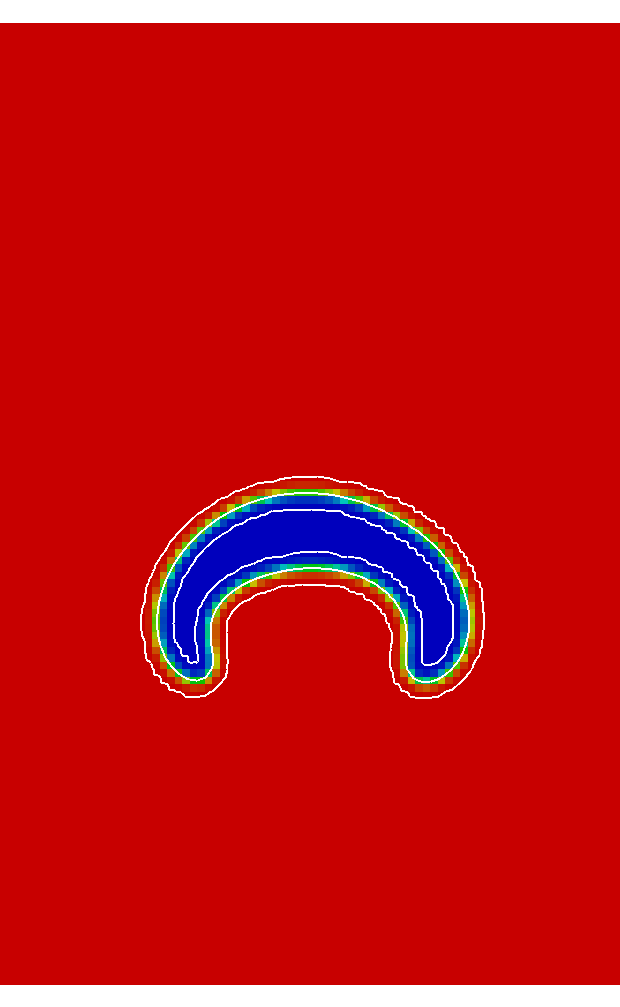
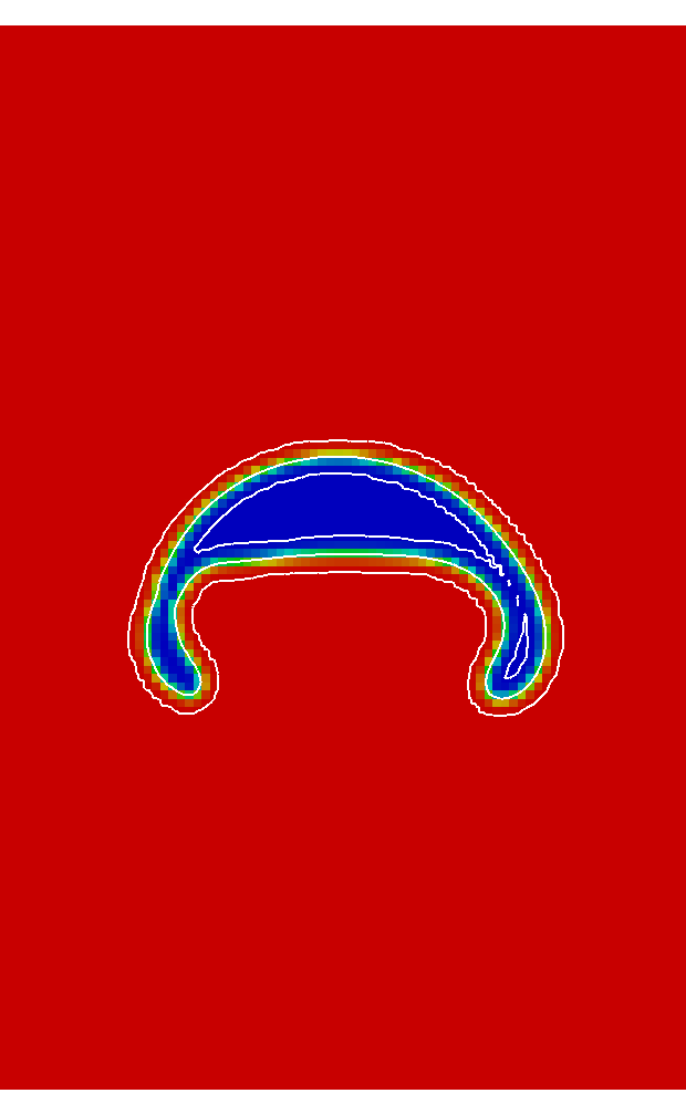
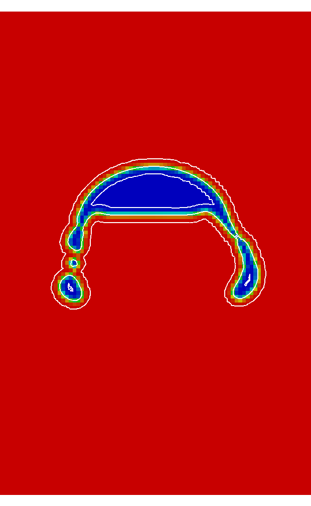
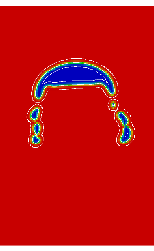
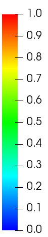
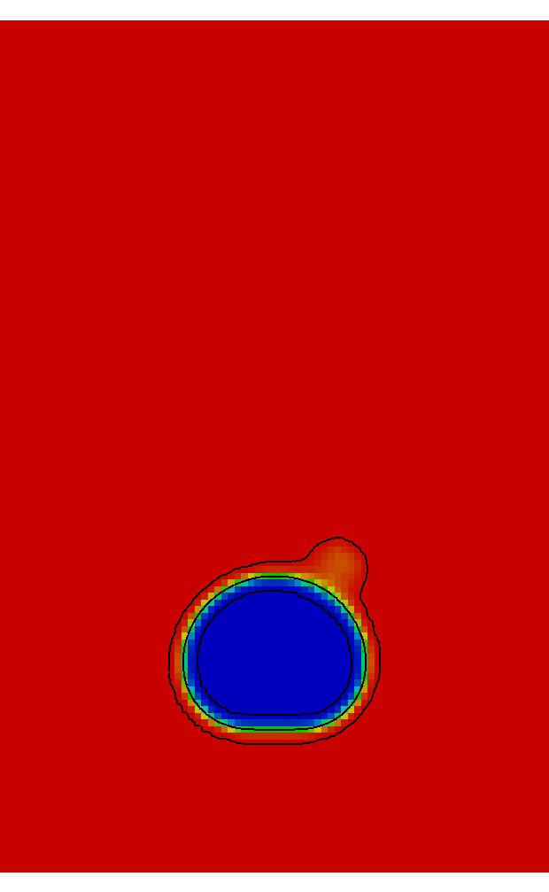
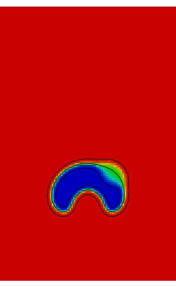
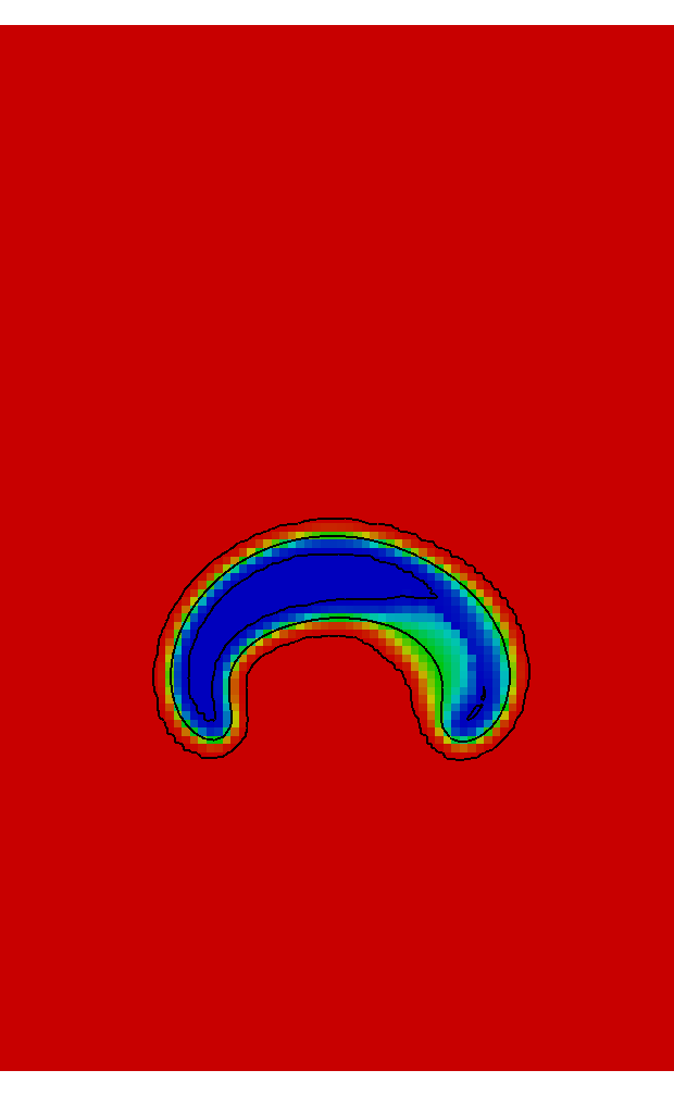
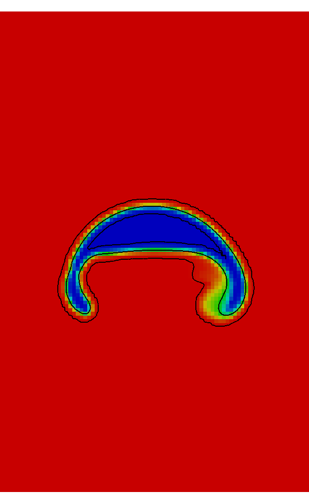
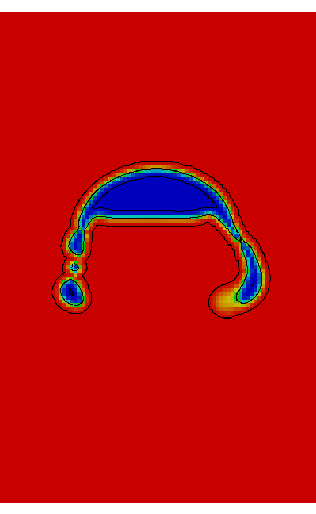
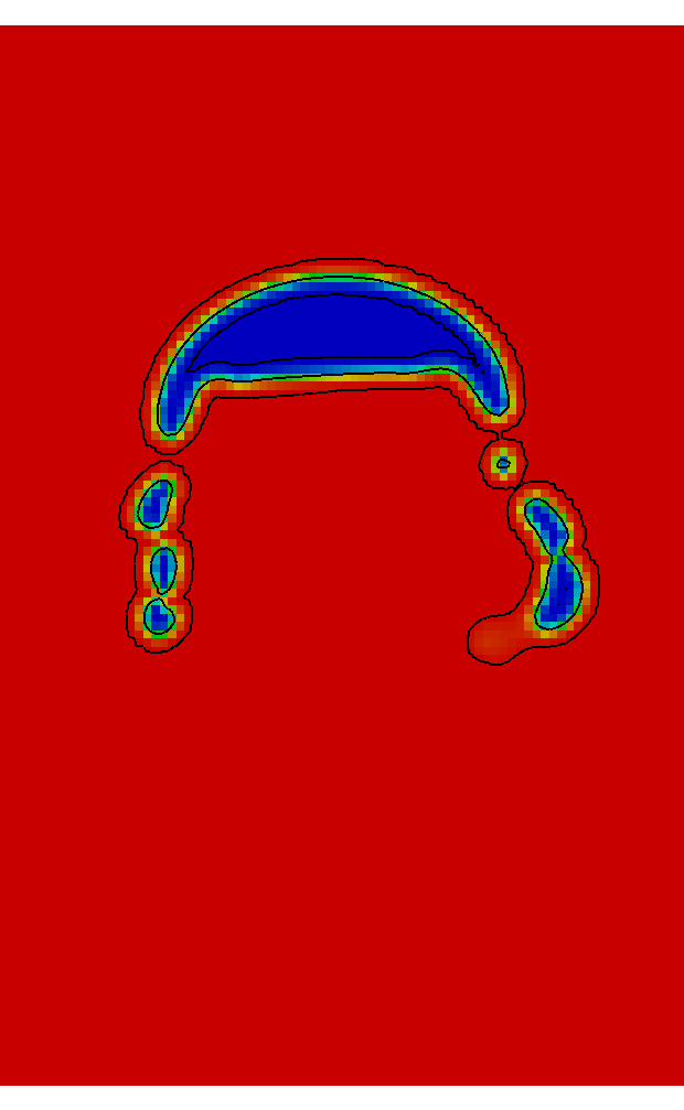
Figure 3: Level-sets $\left[0.01,0.5,0.99\right]$ and color maps of the cumulative distribution functions: $0\!<\!\alpha\left(\psi\right)\!<\!1$ (white contours, top row) and $0\!<\!\alpha_{d}\!\left(\psi\right)\!<\!1$ (black contours, bottom row). Position of both functions is affected by the characteristic length scale field $\epsilon_{h}\left(\mathbf{x},t\right)\,[m]$ with $\epsilon_{h,max}\!=\!11\epsilon_{h,b}\,[m]$, see Fig. 4 (bottom row). The snapshots from the left to the right are taken every $\Delta t\!=\!0.05\,[s]$.

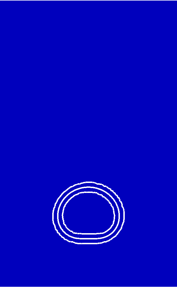
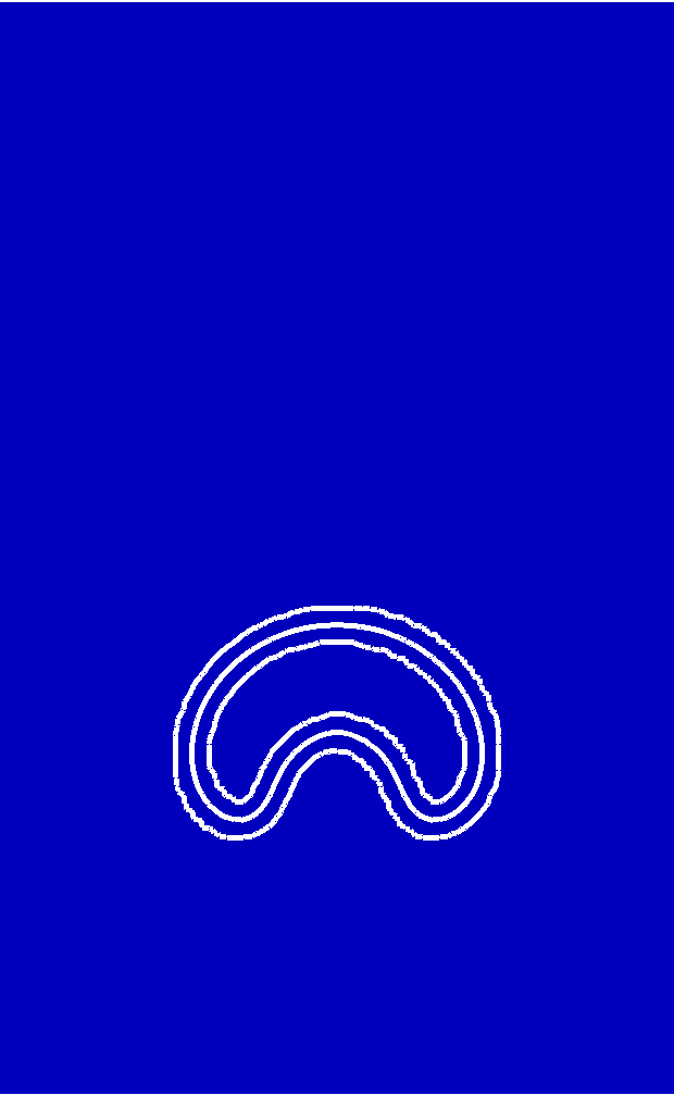
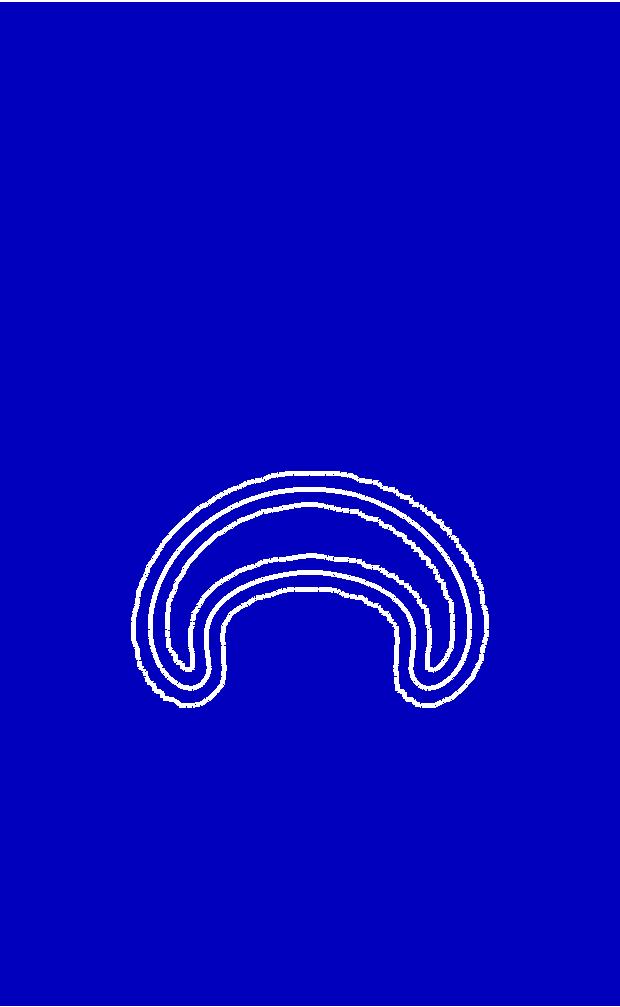
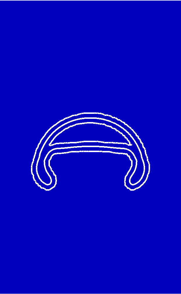
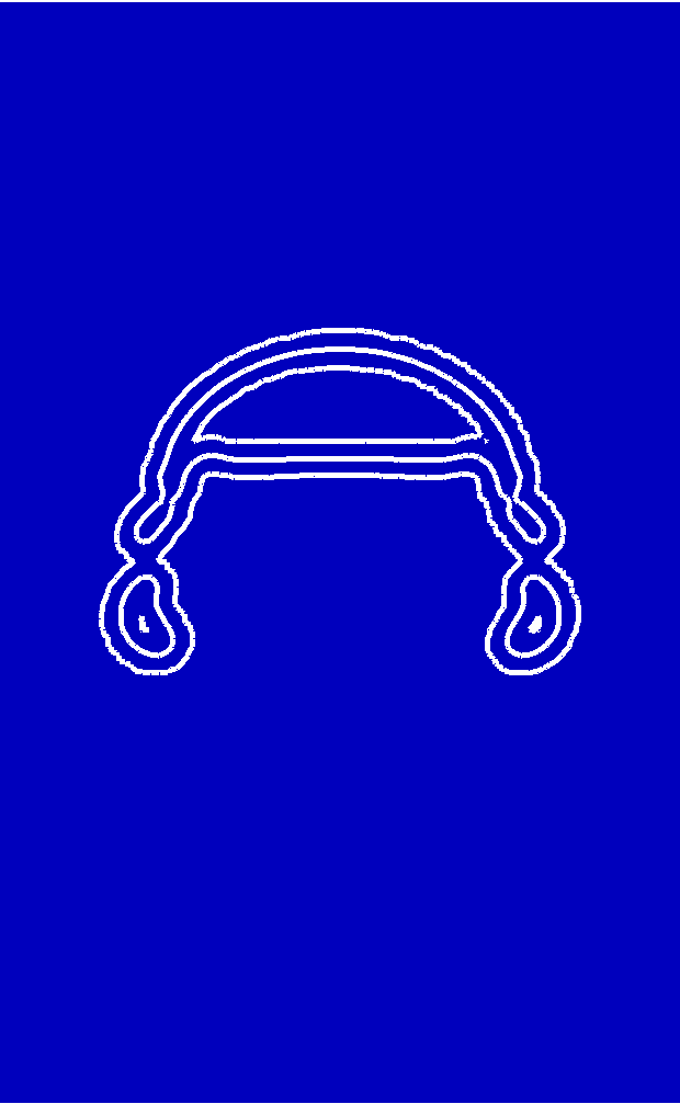
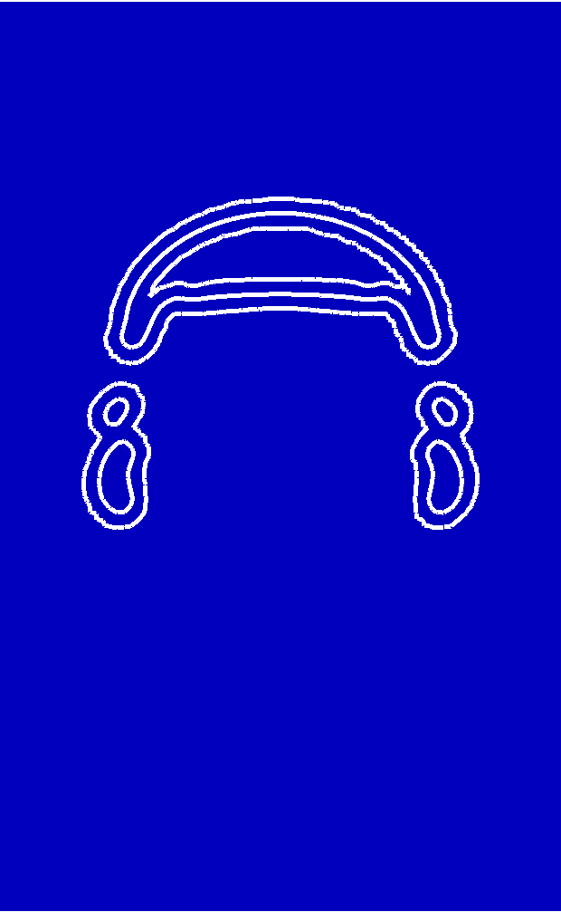
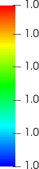
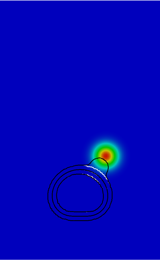
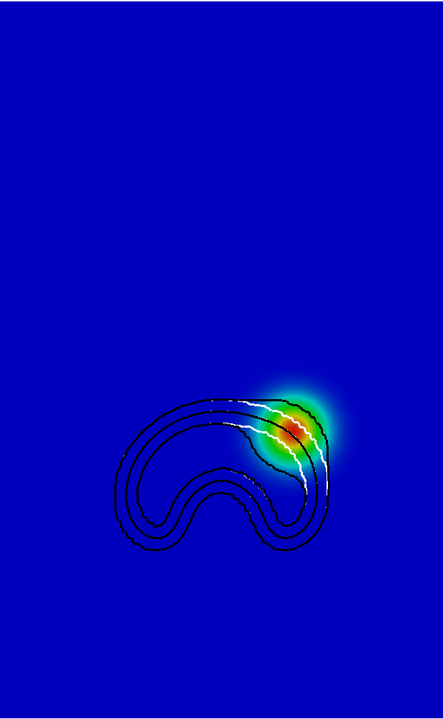
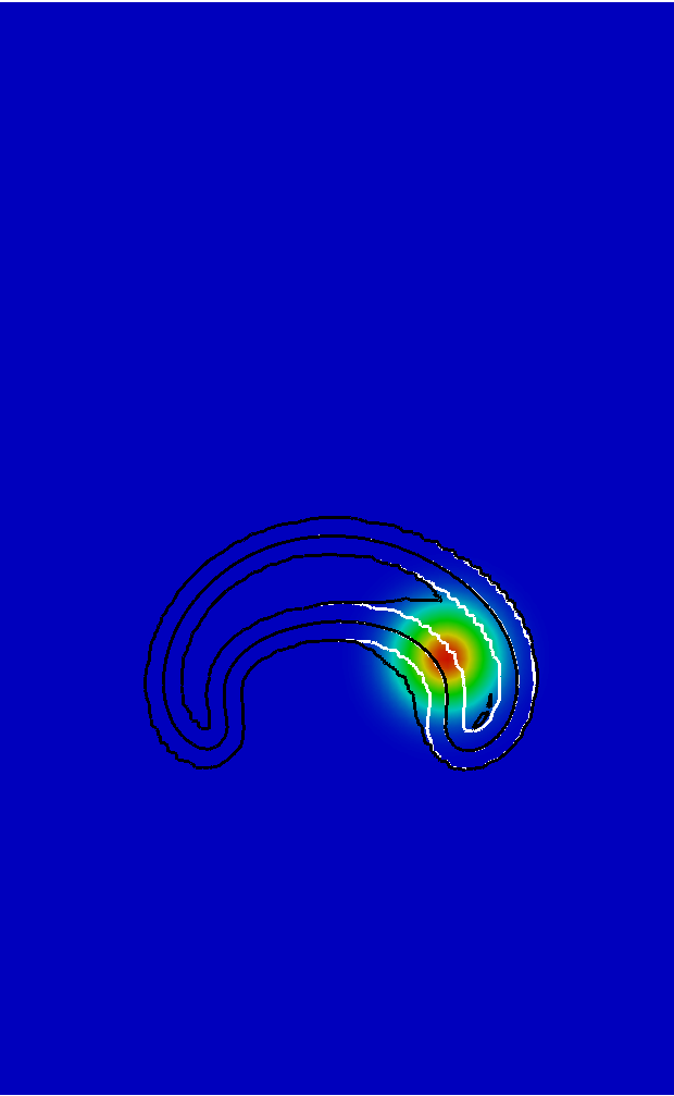
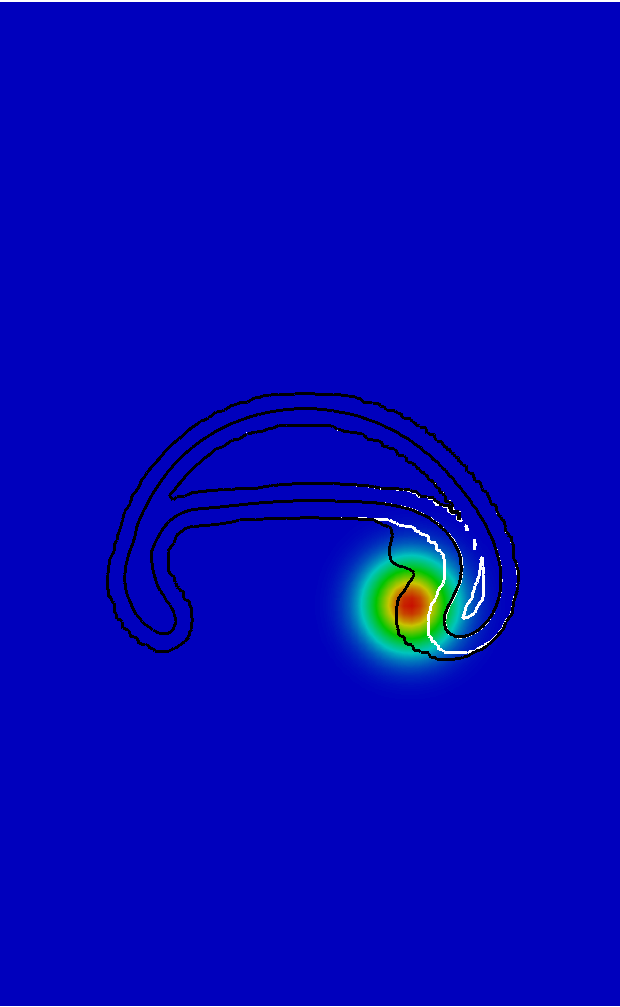
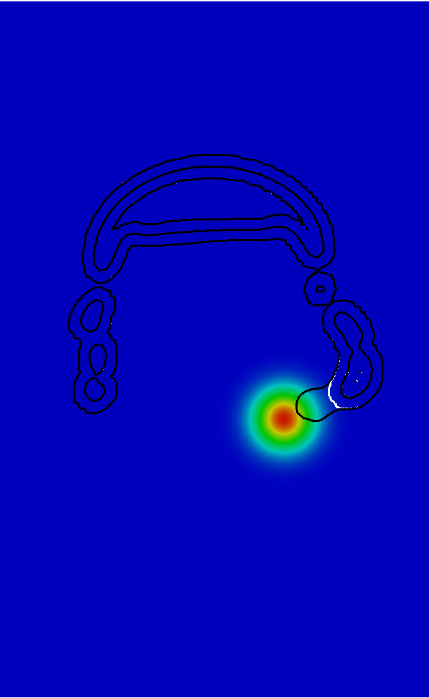
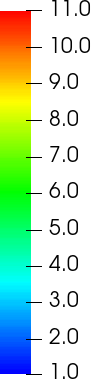
Figure 4: Level-sets $\left[0.01,0.5,0.99\right]$ of the probability $\alpha\left(\psi\right)$ with $\epsilon_{h,b}\!=\!const.$ (white contours) and function $\alpha_{d}\!\left(\psi\right)$ approximating the exact solution of Eq. (9) (black contour). $\alpha_{d}\!\left(\psi\right)$ is affected by the characteristic length scale field $\epsilon_{h}\left(\mathbf{x},t\right)\,[m]$ (colour map). $\epsilon_{h,max}\!=\!\epsilon_{h,b}\!=\!const.$ (top row), $\epsilon_{h,max}\!=\!11\epsilon_{h,b}$ (bottom row). The snapshots from left to right are taken every $\Delta t\!=\!0.05\,[s]$.

3.2 Non-equilibrium effects in the two-phase flow

In the case when $\epsilon_{h}\left(\mathbf{x},t\right)\!=\!const.$, and the regularized interface velocity $\mathbf{w}$ in Eq. (8) is prescribed by known analytical formula, the numerical solution of the transport equations Eqs. (8) and (9) with constraint given by Eq. (4) are described in every detail in twacl15 . In the present work, the non-equilibrium solution of Eq. (9), approximated by Eq. (15) is implemented in described in the previous section two-phase flow solver.

To account for non-equilibrium due to variations in the characteristic length scale field $\epsilon_{h}\left(\mathbf{x},t\right)$, first, Eqs. (8) and (9) are solved with $\epsilon_{h,b}\!=\!const.$, see results presented in the top rows of Figs. 3 – 5 and in the bottom row of Fig. 4 (white contours). This solution provides $\psi\left(\alpha\right)$ and $\alpha\left(\psi\right)$ fields at every time step. Further, $\psi\left(\alpha\right)$ is considered to define the local coordinate systems (where normal in every point of the interface $\gamma:$ $\psi\left(\alpha\!=\!1/2\right)\!=\!0$ is given by $\mathbf{n}_{\gamma}$). These local systems are used to compute the integral Eq. (18) in Eq. (15). The field created by these local coordinate systems is visualized in Fig. 5 as the level-sets of $\psi\left(\alpha\right)$ function.

In twacl21 , physical interpretation of $\psi\left(\alpha\right)$ field was proposed. It is interpreted as the space where the averaged oscillations of the mesoscopic, sharp interface $\Gamma$ take place. The oscillations of $\Gamma$ (in the present work) defined at the molecular level, are governed by thermal fluctuations and for this reason can not be modeled directly in the continuum mechanical description. Eq. (15) mimics their variation in the averaged sense, see twacl21 for full discussion.

Let us consider the last outer iteration of the SIMPLE algorithm, after the single time step $\Delta t\,[s]$ were the momentum conservation and Poisson equations are iterated to enforce stronger coupling between the pressure and velocity fields. At the last outer iteration, $N_{\tau}\!=\!4$ re-initialization steps $\Delta\tau\!=\!D/C^{2}\,[s]$ is carried out advancing Eq. (9) in time $\tau$. As discussed in Section 2.2, this is equivalent to the minimization of the modified Ginzburg-Landau free energy functional.

Before the solution of Eq. (9) in time $\tau$, the integral

$$\begin{split}&\mathcal{I\left(\psi\right)}\!=\!\int^{0}_{1}\frac{dt^{\prime}}{\epsilon_{h}^{t^{\prime}\psi}\!\left(\mathbf{x},t\right)}\!\approx\!\\ &\qquad\qquad\frac{1}{6}\left[\frac{1}{\epsilon_{h}\texttt{(inp)}}+\frac{4}{\epsilon_{h}\texttt{(inm)}}+\frac{1}{\epsilon_{h}\texttt{(int)}}\right].\end{split}$$ (18)

is computed in each control volume (inp) where the signed distance function $\psi\left(\alpha\right)$ is reconstructed. Other Indexes in Eq. (18) denote, respectively, control volumes where: the interface $\alpha\left(\psi\!=\!0\right)\!=\!1/2$ is located (int) and in the distance in between (inm).

It was checked in twacl21 , approximation of the integral (18) using the third-order accurate Simpson rule is sufficient to obtain $\mathcal{I\left(\psi\right)}$ field. Therein, more detailed description of the integration scheme used to evaluate $\mathcal{I\left(\psi\right)}$ field is given, too. Next, obtained in each control volume values of $\mathcal{I\left(\psi\right)}$ are used to compute $\alpha_{d}\!\left(\psi\right)$ field given by Eq. (15) and than material properties are determined setting $\alpha\left(\psi\right)\!=\!\alpha_{d}\!\left(\psi\right)$ in Eqs. (17) and (17). Afterwards, the mass and diffusive fluxes are calculated at the faces of all control volumes. Finally, the segregated Navier-Stokes equation solver proceeds to the solution on the next time step $t\!+\!\Delta t$ solving euqations for velocity components and repeating described procedure.

4 Numerical experiment

In this section, simple two-phase flow experiment is carried out to demonstrate the first application of the numerical method twacl21 used for the approximate solution of Eqs. (4, 8, 9) with Eq. (15) which can account for the non-equilibrium effects due to $\epsilon_{h}\left(\mathbf{x},t\right)\!\neq\!const.$ In particular, during discussion of the numerical results obtained in this study, the differences between statistical and deterministic description of the two-phase flow separated by the intermittency region in the equilibrium or/and non-equilibrium states are emphasized.

4.1 Simulation set-up

In what follows, the two-phase flow of the rising due to positive buoyancy gas bubble is studied. For this demonstration, density and viscosity contrasts are selected to be $\rho_{1}/\rho_{2}\!=\!6$ and $\mu_{1}/\mu_{2}\!=\!20$, respectively. The gravitational acceleration is chosen to have its standard magnitude $\mathbf{g}\!=[0,9.8]\,[m/s^{2}]$. The two-phase flow problem is solved in the domain $\Omega=<0,0.1>\!\times\!<0,0.1>\,[m^{2}]$, discretized using uniform grid with $2^{7}\times 2^{7}$ control volumes. Time step size is set to $\Delta t\!=\!2.5\cdot 10^{-4}\,[s]$ what guarantees the maximum Courant number $Cu_{max}\!<\!0.25\,[-]$ during the whole simulation lasting $T\!=\![0,0.5]\,[s]$.

To couple the pressure and velocity fields, $N_{out}\!=\!4$ outer iterations per time step $\Delta t$ are used. The same time step $\Delta t\,[s]$ is used to advance Eq. (8) in time $t\,[s]$. Re-initialization equation (8) is solved in time $\tau\,[s]$ using the time step size $\Delta\tau\!=\!0.5\!\cdot\!D/C^{2}\!=\!0.5\!\cdot\!\epsilon_{h,b}\,[s]$ and $N_{\tau}\!=\!4$ iterations per $\Delta\tau$. Model function $\alpha_{d}\!\left(\psi\right)$ given by Eq. (15) is computed after each re-initialization cycle.

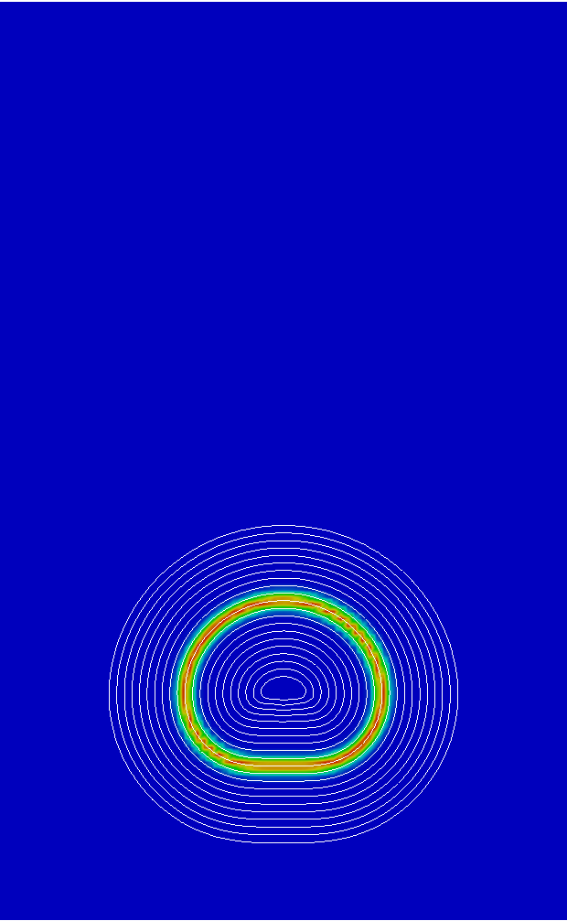
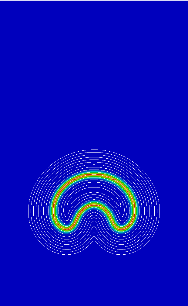
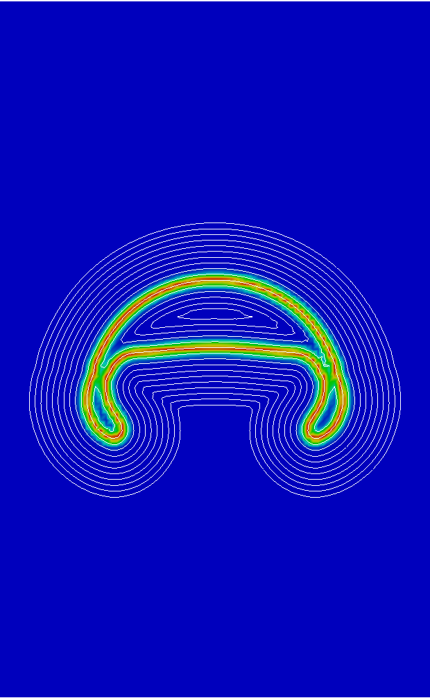
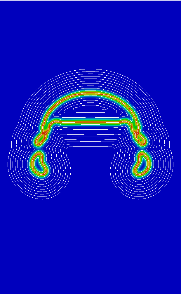
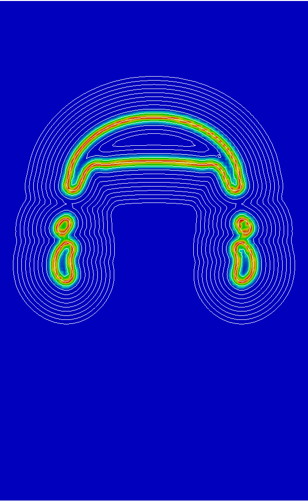
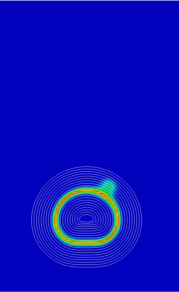
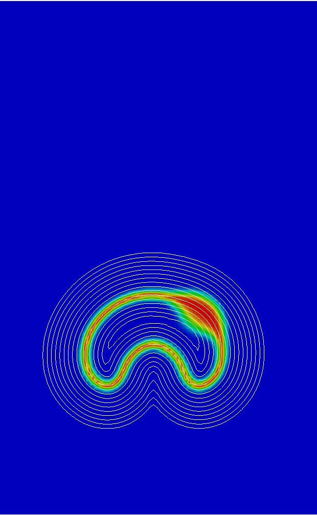
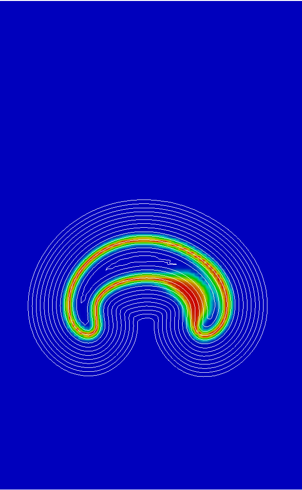
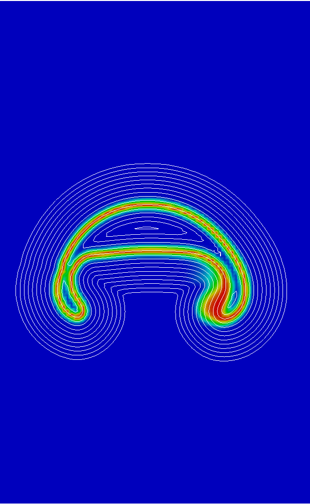
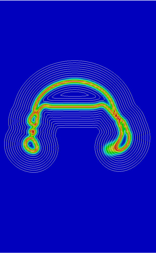
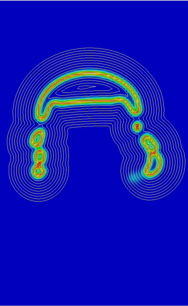
Figure 5: Level-sets $\left\{-3\!\cdot\!n\!\cdot\!\epsilon_{h,b},0,3\!\cdot\!n\!\cdot\!\epsilon_{h,b}\right\}$ where $n\!=\!1,\ldots,8$ of the signed distance function field $\psi\left(\alpha\right)$. The color map depicts joint probability $\alpha_{d}\!\left(\psi\right)\left(1\!-\!\alpha_{d}\!\left(\psi\right)\right)$ of finding the phase $\alpha_{d}\!\left(\psi\right)$ used to define the macroscopic interface $\gamma$ position. $\epsilon_{h,max}\!=\!\epsilon_{h,b}\!=\!const.$ (top row), $\epsilon_{h,max}\!=\!11\epsilon_{h,b}$ (bottom row). The snapshots from the left to the right are taken every $\Delta t\!=\!0.05\,[s]$.

In Fig. 1, sketch of the computational domain with the initial position of the gas bubble $[0.05,0.02]\,[m]$ having diameter $D\!=\!0.02\,[m]$ is presented. The same figure depicts constant in time position $\mathbf{x}_{r}\!=\![0.06,0.04]\,[m]$ of the maximal value of the characteristic length scale field $\epsilon_{h}\left(\mathbf{x},t\right)$ (colored drop), see also the color map in Fig. 4.

The spatial variation of the characteristic length scale field $\epsilon_{h}\left(\mathbf{x},t\right)$ is predefined to be bell shaped with the analytical formula

$$\epsilon_{h}\left(\mathbf{x},t\right)\!=\!\epsilon_{h,b}\left\{1+A\!\cdot\!\exp{\left[-\left(\frac{r}{20\epsilon_{h,b}}\right)^{2}\right]}\right\}$$ (19)

where $r\!=\!\left[\left(x-x_{r}\right)^{2}+\left(y-y_{r}\right)^{2}\right]^{1/2}$, $\mathbf{x}_{r}$ denotes center of $\epsilon_{h}\left(\mathbf{x},t\right)$, and the base width of the intermittency region is $\epsilon_{h,b}=\sqrt{2}\Delta x/4$.

To analyze influence of $\epsilon_{h}\left(\mathbf{x},t\right)$ magnitude on the obtained results, in particular on the mass conservation computed using $\alpha\left(\psi\right)$ or $\alpha_{d}\!\left(\psi\right)$ functions several values of $A\!=\!\left\{2.5,5.0,7.5,10\right\}$ are used affecting the maximal elevation of $\epsilon_{h}\left(\mathbf{x},t\right)$ field. These $A$ values, result in $\epsilon_{h,max}\!=\!max\left[\epsilon_{h}\left(\mathbf{x},t\right)\right]\!=\!\left\{3.5,6,8.5,11\right\}$ elevations, see results in Fig. 2.

It is noticed, Figs. 3 – 5 show only the results of numerical simulation in the two cases $\epsilon_{h,max}/\epsilon_{h,b}\!=\!\left\{1,\,11\right\}$. When $\epsilon_{h,max}/\epsilon_{h,b}\!=\!1$ than $\epsilon_{h}\left(\mathbf{x},t\right)=const.$; in the case $\epsilon_{h,max}/\epsilon_{h,b}\!=\!11$, $\epsilon_{h}\left(\mathbf{x},t\right)$ is defined by Eq. (19) with $A=10$.

5 Discusion of the results

5.1 Conservation of mass

At first the mass conservation of the present numerical method is discussed, see Fig. 2. As in the present model we are using the functions $\alpha\left(\psi\right)$ (in the equilibrium case when $\epsilon_{h}\left(\mathbf{x},t\right)\!=\!\epsilon_{h,b}\!=\!const.$) and $\alpha_{d}\!\left(\psi\right)$ (to account for variations in $\epsilon_{h}\left(\mathbf{x},t\right)$ field), they both can be used to compute conservation of mass or area in incompressible two-phase flow. In the statistical interpretation, the mass conservation is equivalent of the probability (of finding phase chosen to identify the macroscopic interface $\gamma$) conservation.

In Fig. 2 history of the mass variation in the present test case is presented. This diagram is obtained using integration of $\alpha\left(\psi\right)$, $\alpha_{d}\!\left(\psi\right)$ functions in the computational domain there where $\psi\left(\alpha\right)$ is reconstructed. It is noted, the total mass/area is slightly higher then $S_{ext}=\pi D^{2}/4$ used to normalize data in Fig. 2. This is because $\alpha\left(\psi\right)$, $\alpha_{d}\!\left(\psi\right)$ are the cumulative distribution functions with the infinite support and they are resolved that way as accurate as it is possible with the double precision computer arithmetic. In both cases presented in Fig. 2 the law of mass conservation is satisfied during the whole simulation. In this test, the coarse mesh is used ($\sim 26$ grid nodes per buble diameter $D$ at $t=0\,[s]$), the relatively exact mass conservation is due to the conservative form of the transport Eq. (7).

In the case of the mass recording obtained using $\alpha\left(\psi\right)$ in Fig. 2 (left) one observes how coupling through continuity equation with the non-equilibrium solution affects its conservation. Counter intuitively, the larger $\epsilon_{h}\left(\mathbf{x},t\right)$ field magnitude $\epsilon_{h,max}$ is, the lower mass error is obtained.

In Fig. 2 (right), conservation of $\alpha_{d}\!\left(\psi\right)$ is depicted. Herein, one notes interaction with the variable characteristic length scale field $\epsilon_{h}\left(\mathbf{x},t\right)$ causes fluctuations of the mass magnitude in $\pm 3\%$ range. However, due to coupling with the conserved $\alpha\left(\psi\right)-\psi\left(\alpha\right)$ functions the total mass is conserved as well.

The time moments of oscillations peaks in Fig. 2 (right) can be compared with the two-phase flow field(s) in Figs. 3 – 5. One can observe, these peaks occur when the non-symmetrical modes of $\alpha_{d}\!\left(\psi\right)$ are induced by $\epsilon_{h}\left(\mathbf{x},t\right)$ field. This can be obseved at times $t=0.015,0.02\,[s]$, e.g. compare results in Fig. 2 and Fig. 3.

5.2 Impact of non-equilibrium effects on two-phase flow

Impact of the characteristic length scale field $\epsilon_{h}\left(\mathbf{x},t\right)$ on the obtained results is presented in Figs. 4 – 5, compare results in the top and bottom rows. One observes, in the case $\epsilon_{h}\left(\mathbf{x},t\right)=\epsilon_{h,b}$ investigated two-phase flow is symmetric. In spite they are there, black contours of $\alpha_{d}\!\left(\psi\right)$ field can not be seen in Fig. 4 (top row) because in this case $\alpha_{d}\!\left(\psi\right)\!=\!\alpha\left(\psi\right)$.

This is not the case in the bottom row of Fig. 4. Herein, the difference between $\alpha\left(\psi\right)$ (white contours) and $\alpha_{d}\!\left(\psi\right)$ (black contours) functions is clearly visible. As in the non-equilibrium case, the material properties of gas and liquid phases are computed using Eqs. (15) and (17) with $\alpha\left(\psi\right)$ replaced by $\alpha_{d}\!\left(\psi\right)$. This locally changes the mass and diffusive fluxes used to solve the Navier-Stokes equations and couple the pressure and velocity fields. Therefore now, the two-phase flow scenario is affected by $\alpha_{d}\!\left(\psi\right)$ variations causing the flow symmetry to be broken. This can be attributed to differences in topological changes on the left and right side of the gas bubble, compare results in the top and bottom rows in Figs. 4 – 5 for example at times $t=0.25,\,0.3\,[s]$.

In our opinion, the best illustration of mechanisms in the statistical two-phase flow model is given by the joint probabilities $\alpha\left(\psi\right)\left(1-\alpha\left(\psi\right)\right)$ or $\alpha_{d}\!\left(\psi\right)\left(1-\alpha_{d}\!\left(\psi\right)\right)$ depicted in the top and bottom rows in Fig. 5, respectively. Variations of the joint probability used to identify macroscopic interface $\gamma$ as $\psi\left(\alpha=1/2\right)=0$, illustrate the probability distribution of the mesoscopic interface $\Gamma$ residence. In other words, in regions with higher joint probability, it is more likely to find the mesoscopic interface $\Gamma$ (we recall in the present work $\Gamma$ is defined on the molecular level).

5.3 Difference between statistical and deterministic two-phase flow models

Finally, let us discuss the main difference between deterministic and statistical mwaclawczyk11 ; waclawczyk2015 ; twacl15 ; twacl17 ; twacl21 two-phase flow models used in the one-fluid model framework.

In the deterministic description of the interface, the physical interpretation is attributed only to flow domains where the order parameter or the phase indicator function has value zero or one trygg11 ; kim12 . According to models of Gibbs gibbs1874 and van der Waals waals1979 , these domains are occupied by the homogeneous gas or liquid phases lang15 . However, in physical/chemical reality, gases or liquids will never be homogeneous (gas or liquid phases containing 100% of one type molecules are almost never observed in every day experience). Moreover, this constraint imposed on the deterministic sharp interface models results in the presumption that domains where the numerical solution of the order parameter or phase indicator transport equation is between zero and one (smeared, not sharply resolved regions) are non-physical. Similarly, diffusive interface in the phase field models is considered to be thin transition region between the two-phases without clear physical interpretation as well. Nevertheless, exceptionally, the position of the interface in its sharp and/or diffusive deterministic models is typically located between zero and one. As a consequence, the only possibility to increase the accuracy of the numerical predictions with the sharp or diffusive interface model(s) is addition of the new grid points using the adaptive refinement what impairs performance of the solver (steam is putted to the wrong, non-physical wheel).

In the statistical model of intermittency region, the cumulative distribution function describing the probability of finding mesoscopic interface $\Gamma$ (or probability of finding the phase chosen to identify $\Gamma$ and $\gamma$) is bounded $0\!<\!\alpha\left(\psi\right)\!<\!1$ and conserved from its definition, see mathematical form of Eq. (7). In this interpretation, the expected position of the interface $\Gamma$ defined as $\alpha\left(\psi\!=\!0\right)\!=\!1/2$ explains where the macroscopic interface $\gamma$ is located (also in the deterministic interface models). Moreover, values of $\alpha\left(\psi\right)$ have the physical interpretation over the entire range of $\alpha\left(\psi\right)$ field magnitude. Hence, regions where the two-phase flow is not resolved due to lack of the spatial resolution are promoted to physical interpretation as well. This feature of the statistical model of the intermittency region is general and applies equally to the equilibrium and non-equilibrium flow cases. In order not to be too vague, let us analyze the results obtained in the present numerical experiment in the context of above explanations.

It is recalled, $\alpha\left(\psi\right)$ and $\alpha_{d}\!\left(\psi\right)$ are probabilities of finding the liquid phase, $1\!-\!\alpha\left(\psi\right)$ and $1\!-\!\alpha_{d}\!\left(\psi\right)$ are probabilities of finding the gas phase. We note, at $t=0.3\,[s]$ (see Figs. 3 – 5) some features of the rising gas bubble are not well resolved. Contours of $\alpha\left(\psi\right)$ (white) and $\alpha_{d}\!\left(\psi\right)$ (black) capture only values $\left\{0.5,0.99\right\}$, see Figs. 3 – 4. Unlike in the deterministic interface models, the present numerical solution, although not fully resolved, still carries a physical information. Namely it means, that finding of the gas phase in such regions is not certain as $1\!-\!\alpha\left(\psi\right)\!<\!0.99$ and this is why $\alpha\left(\psi\right)\!=\!0.01$ or $\alpha_{d}\!\left(\psi\right)\!=\!0.01$ contours can not be seen.

6 Conclusions

In the present paper, the statistical model of the intermittency region between two phases twacl17 ; twacl21 was coupled with the incompressible Navier-Stokes equation solver to study differences between the equilibrium and non-equilibrium solution of Eq. (7) in the case of rising gas bubble. Results of the present numerical simulations show, inclusion of recently proposed approximate solution to Eq. (7) permits to account for non-equilibrium effects in the two-phase flow model rooted in the one-fluid framework.

Moreover, we have discussed differences between deterministic sharp and diffusive interface models and statistical interface model. It is concluded, the main difference between these two descriptions of two-phase flow is that the results of the statistical two-phase flow model can be interpreted over the entire range of the cumulative distribution function $\alpha\left(\psi\right)$ values also when two-phase flow is not fully resolved.

References

- (1) Anderson, D.M., McFadden, G.B., Wheeler, A.A.: Diffuse-Interface Methods in Fluid Mechanics. Annu. Rev. Fluid Mech. 30(1), 139–165 (1998)
- (2) Osher, S., Fedkiw, R.: Level Set Methods and Dynamic Implicit Surfaces. Springer Verlag, INC. New-York (2003)
- (3) Prosperetti, A., Grétar, T.: Computational Methods for Multiphase Flow. Cambridge University Press (2006)
- (4) Tryggvason, G., Scardovelli, R., Zaleski, S.: Direct Numerical Simulations of Gas-Liquid Multiphase Flows. Cambridge University Press (2011)
- (5) Kim, J.: Phase-field models for multi-component fluid flows. Communications in Computational Physics 12(3), 613–661 (2012)
- (6) Allen, S., Cahn, J.: A microscopic theory for antiphase domain boundary motion and its application to antiphase domain coarsening. Acta Metall. 27, 1085–1095 (1979)
- (7) Cahn, J.W., Hilliard, J.E.: Free Energy of a Nonuniform System. I. Interfacial Free Energy. J. Chem. Phys. 28(2), 258–267 (1958)
- (8) Kim, J., Lee, S., Choi, Y.: A conservative Allen-Cahn equation with a spacetime dependent Lagrange multiplier. Int. J. Eng. Sci. 84, 11 – 17 (2014)
- (9) Gibbs, J.W.: On the equilibrium of heterogeneous substances. Academy (1874)
- (10) van der Waals, J.: The thermodynamic theory of capillarity under the hypothesis of a continuous variation of density. J. Statist. Phys. 20(2), 200–244 (1979)
- (11) Láng, G.G.: Basic interfacial thermodynamics and related mathematical background. ChemTexts 1(3), 1–16 (2015)
- (12) Faust, J.A.: Foreword. In: J.A. Faust, J.E. House (eds.) Physical Chemistry of Gas-Liquid Interfaces, Developments in Physical & Theoretical Chemistry, pp. Foreword, xvii. Elsevier (2018). DOI https://doi.org/10.1016/B978-0-12-813641-6.12001-1. URL http://www.sciencedirect.com/science/article/pii/B9780128136416120011
- (13) Liu, X.D., Osher, S., Chan, T.: Weighted essentially non-oscillatory schemes. Journal of Computational Physics 115(1), 200–212 (1994)
- (14) Cummins, S.J., Francois, M.M., Kothe, D.B.: Estimating curvature from volume fractions. Computers & Structures 83(6), 425–434 (2005), frontier of Multi-Phase Flow Analysis and Fluid-Structure
- (15) Popinet, S.: An accurate adaptive solver for surface-tension-driven interfacial flows. Journal of Computational Physics 228, 5838–5866 (2009)
- (16) Vrij, A.: Light scattering from liquid interfaces. Chemie Ingenieur Technik 45(18), 1113–1114 (1973)
- (17) Aarts, D.G.A.L., Schmidt, M., Lekkerkerker, H.N.W.: Direct visual observation of thermal capillary waves. Science 304(5672), 847–850 (2004)
- (18) Hirt, C.W., Nichols, B.D.: Volume of fluid (VOF) method for dynamics of free boundaries. Journal of Computational Physics 39, 201–225 (1981)
- (19) Osher, S., Sethian, J.A.: Fronts propagating with curvature-dependent speed: Algorithms based on Hamilton-Jacobi formulations. J. Comp. Phys. 79(1), 12 – 49 (1988)
- (20) Olsson, E., Kreiss, G.: A conservative level-set method for two phase flow. J. Comp. Phys. 210, 225–246 (2005)
- (21) Wacławczyk, T.: On a relation between the volume of fluid, level-set and phase field interface models. International Journal of Multiphase Flow 97, 60 – 77 (2017)
- (22) Wacławczyk, T.: A consistent solution of the re-initialization equation in the conservative level-set method. J. Comp. Phys. 299, 487 – 525 (2015)
- (23) Wacławczyk, T.: Modeling of non-equilibrium effects in intermittency region between two phases. International Journal of Multiphase Flow 134, 103459 (2021)
- (24) Brocchini, M., Peregrine, D.H.: The dynamics of strong turbulence at free surfaces. Part 1. Description. J. Fluid Mech. 449, 225–254 (2001)
- (25) Wacławczyk, M., Oberlack, M.: Closure proposals for the tracking of turbulence-agitated gas-liquid interfaces in stratified flows. Int. J. Multiphase Flow 37, 967–976 (2011)
- (26) Wacławczyk, M., Wacławczyk, T.: A priori study for the modelling of velocity-interface correlations in the stratified air-water flows. Int. J. Heat Fluid Flow 52(0), 40 – 49 (2015)
- (27) Pope, S.: The evolution of surfaces in turbulence. Int. J. Eng. Sciences 26, 445–469 (1998)
- (28) Chiu, P.H., Lin, Y.T.: A conservative phase field method for solving incompressible two-phase flows. J. Comp. Phys. 230(1), 185–204 (2011)
- (29) Kraheberger, S.V., Wacławczyk, T., Wacławczyk, M.: Numerical study of the intermittency region in two-fluid turbulent flow. In: Progress in Turbulence VI, Proceedings of the iTi Conference on Turbulence 2014, pp. 289–293. Bertinoro, Italy (2014)
- (30) Wacławczyk, T., Wacławczyk, M., Kraheberger, S.V.: Modeling of turbulence-interface interactions in stratified two-phase flows. Journal of Physics: Conference Series 530 (2014)
- (31) Dadvand, A., Bagheri, M., Samkhaniani, N., Marschall, H., Wörner, M.: Advected phase-field method for bounded solution of the cahn–hilliard navier–stokes equations. Physics of Fluids 33(5), 053311 (2021)
- (32) Mirjalili, S., Ivey, C.B., Mani, A.: A conservative diffuse interface method for two-phase flows with provable boundedness properties. Journal of Computational Physics 401, 109006 (2020)
- (33) Ascher, M., Petzold, L.: Computer Methods for Ordinary Differential Equations and Differential-Algebraic equations. Sociaty for Industrial and Applied Mathematics (1998)
- (34) Folch, R., Casademunt, J., Hernández-Machado, A., Ramírez-Piscina, L.: Phase-field model for hele-shaw flows with arbitrary viscosity contrast. i. theoretical approach. Phys. Rev. E 60, 1724–1733 (1999)
- (35) Jamet, D., Misbah, C.: Thermodynamically consistent picture of the phase-field model of vesicles: Elimination of the surface tension. Phys. Rev. E 78, 041903 (2008)
- (36) Schäfer, M.: Computational Engineering, Introduction to Numerical Methods. Springer-Verlag Berlin Heidelberg New York (2006)
- (37) Ferziger, J.H., Perić, M.: Computational Methods for Fluid Dynamics. Springer Verlag, Berlin Heidelberg New York (2002)
- (38) Wacławczyk, T., Koronowicz, T.: Modelling of the flow in systems of immiscible fluids using Volume of Fluid method with CICSAM scheme. Int. J. Turbulence 11, 267–276 (2005)
- (39) Wacławczyk, T., Koronowicz, T.: Modelling of the free surface flows with high-resolution schemes. Chemical and Process Engineering 27, 783–802 (2006)
- (40) Wacławczyk, T., Gemici, Ö.C., Schäfer, M.: Novel high-resolution scheme for interface capturing. In: Proceedings of the 6-th International Conference on Multiphase Flow, ICMF 2007. Leipzig, Germany (2007)
- (41) Wacławczyk, T., Koronowicz, T.: Remarks on prediction of wave drag using VOF method. Archives of Civil and Mechanical Engineering 8, 6–14 (2008)
- (42) Wacławczyk, T., Koronowicz, T.: Comparison of CICSAM and HRIC high resolution schemes for interface capturing. J. Theoretical and Applied Mechanics 46, 325–345 (2008)
- (43) Wacławczyk, T., Koronowicz, T.: Remarks on prediction of wave drag using VOF method with interface capturing approach. Archives of Civil and Mechanical Engineering 8(1), 5 – 14 (2008)
- (44) Wacławczyk, T.: Numerical modelling of free surface flows in ship hydrodynamics. Ph.D. thesis, Institute of Fluid Flow Machinery, Gdańsk, Poland (2008)
- (45) Mencinger, J., Zun, I.: On the finite volume discretization of discontinuous body force field on collocated grid. Journal of Computational Physics 221, 524–538 (2007)
- (46) Xue, L.: Entwicklung eines effizenten parallelen lösungsalgorithmus zur dreidimenisonalen simulation komplexer turbulenter strömungen. Ph.D. thesis, Doktorarbeit, Technische Universität Berlin (1998)
- (47) Gottlieb, S., Shu, C.W.: Total variation diminishing Runge-Kutta schemes. Math. Comp. 67, 73–85 (1998)