SPATE-GAN: Improved Generative Modeling of Dynamic Spatio-Temporal Patterns with an Autoregressive Embedding Loss

Abstract

From ecology to atmospheric sciences, many academic disciplines deal with data characterized by intricate spatio-temporal complexities, the modeling of which often requires specialized approaches. Generative models of these data are of particular interest, as they enable a range of impactful downstream applications like simulation or creating synthetic training data. Recent work has highlighted the potential of generative adversarial nets (GANs) for generating spatio-temporal data. A new GAN algorithm COT-GAN, inspired by the theory of causal optimal transport (COT), was proposed in an attempt to better tackle this challenge. However, the task of learning more complex spatio-temporal patterns requires additional knowledge of their specific data structures. In this study, we propose a novel loss objective combined with COT-GAN based on an autoregressive embedding to reinforce the learning of spatio-temporal dynamics. We devise SPATE (spatio-temporal association), a new metric measuring spatio-temporal autocorrelation by using the deviance of observations from their expected values. We compute SPATE for real and synthetic data samples and use it to compute an embedding loss that considers space-time interactions, nudging the GAN to learn outputs that are faithful to the observed dynamics. We test this new objective on a diverse set of complex spatio-temporal patterns: turbulent flows, log-Gaussian Cox processes and global weather data. We show that our novel embedding loss improves performance without any changes to the architecture of the COT-GAN backbone, highlighting our model’s increased capacity for capturing autoregressive structures. We also contextualize our work with respect to recent advances in physics-informed deep learning and interdisciplinary work connecting neural networks with geographic and geophysical sciences.

Introduction

Over the last decade, deep learning has emerged as a powerful paradigm for modeling complex data structures. It has also found successful applications in the video domain, for example for trajectory forecasting, video super-resolution or object tracking. Nevertheless, data observed over (discrete) space and time can take many more shapes than just RGB videos: many of the systems and processes governing our planet, from ocean streams to the spread of viruses, exhibit complex spatio-temporal dynamics. Current deep learning approaches often struggle to account for these, as a recent survey by Reichstein et al. (2019) highlights. The authors call for more concerted research efforts aiming to improve the capacity of deep neural networks for modeling earth systems data. Recently, the emergence of physics-informed deep learning has reinforced the integration of physical constraints as a research domain (Zhang and Zhao 2021; Rao, Sun, and Liu 2020; Wang et al. 2020b; Kim et al. 2020).

In this work, we propose a novel GAN tailored to the challenges of spatio-temporal complexities. We first devise a novel measure of spatio-temporal association—SPATE—expanding on the Moran’s I measure of spatial autocorrelation. SPATE uses the deviance of an observation from its space-time expectation, and compares it to neighboring observations to identify regions of (relative) change and regions of (relative) homogeneity over time. We propose three different approaches to calculate the space-time expectations, coming with varying assumptions and advantages for different applications. We then encode a SPATE-based embedding into COT-GAN (Xu et al. 2020) to formulate a new GAN framework, named SPATE-GAN. The motivation of choosing COT-GAN as the base model is that its principle of respecting temporal dependencies in sequential modeling is in line with our intuition for SPATE, see details in the methods section. Lastly, we test our approach on a range of different datasets. Specifically, we select data characterized by complex spatio-temporal patterns such as fluid dynamics (Wallace 2014; Wang et al. 2020b), disease spread (Brix and Diggle 2001) or global surface temperatures (Sismanidis et al. 2018). We observe that SPATE-GAN outperforms baseline models. This finding is particularly interesting as we do not change the architecture of the existing COT-GAN backbone, implying that our performance gains can be solely attributed to our novel SPATE-based embedding loss.

To summarize, the contributions of this study are as follows:

• We introduce SPATE, a new measure of spatio-temporal association, by expanding the intuition of the Moran’s I metric into the temporal dimension.

• We introduce SPATE-GAN, a novel GAN for complex spatio-temporal data utilizing SPATE to construct an embedding loss ”nudging” the model to focus on the learning of autoregressive structures.

• We test SPATE-GAN against baseline GANs designed for image/video generation on datasets representing fluid dynamics, disease spread and global surface temperature. We show performance gains of SPATE-GAN over the baseline models.

Related work

Autocorrelation metrics for spatio-temporal phenomena

Analysing autoregressive patterns in spatial and spatio-temporal data has a long tradition in different academic domains (e.g. GIS, ecology) which over time developed diverse measures to describe these phenomena. The most commonly known of these metrics is the Moran’s I index of global and local spatial autocorrelation. Originally proposed by Anselin (1995), Moran’s I identifies both homogeneous spatial clusters and outliers. Applications of the metric range from identifying rare earth contamination (Yuan, Cave, and Zhang 2018) to analysing land cover change patterns (Das and Ghosh 2017). Throughout the years, Moran’s I has also motivated several methodological expansions, analysing for example spatial heteroskedasticity (Ord and Getis 2012) and local spatial dispersion (Westerholt et al. 2018). Moran’s I has also seen some expansions into the spatio-temporal domain. Matthews, Diawara, and Waller (2019) use the metric iteratively to model disease spread over time. Lee and Li (2017) and Gao et al. (2019) propose novel spatio-temporal expansions of the Moran’s I metric, returning static outputs at a purely spatial resolution. Siino et al. (2018) design an extended Moran’s I for spatio-temporal point processes. However, to the best of our knowledge, neither the Moran’s I nor its spatio-temporal extensions have been applied to discrete spatio-temporal video data. It is evident that metrics of spatio-temporal autocorrelation can provide meaningful embeddings of complex data, capturing underlying patterns throughout a range of different application domains.

Deep learning & GANs for spatial and spatio-temporal data

Deep learning describes a powerful family of methods capable of dealing with the highly complex and non-linear nature of many real world spatial and spatio-temporal patterns (Yan et al. 2017; Aodha, Cole, and Perona 2019; Chu et al. 2019; Bao et al. 2020; Geng et al. 2019). Paradigms like physics-informed deep learning aim to devise methods which integrate (geo)physical constraints explicitly into neural network models (Wang et al. 2020b). There is also an increasing number of studies tackling specific challenges associated with geographic data: Mai et al. (2020) and Yin et al. (2019) propose context-aware vector embeddings for geographic coordinates. Zammit-Mangion et al. (2019) propose to learn deep neural networks for spatial covariance patterns using injective warping functions. Intuitions for spatial autocorrelation, including the Moran’s I metric, have been integrated into machine learning frameworks tackling model selection for ensemble learners (Klemmer, Koshiyama, and Flennerhag 2019), spatial representation learning (Zhang et al. 2019), auxiliary task learning (Klemmer and Neill 2021) or residual correlation graph neural networks (Jia and Benson 2020). All these studies highlight the benefits of explicitly encoding spatial context into neural networks to improve performance.

Narrowing down on the GAN context specifically, we find that spatio-temporal applications have mostly focused on video data (Xu et al. 2020; Tulyakov et al. 2018; Kim, Oh, and Kim 2020). Beyond this, GANs have been used for conditional density estimation of traffic (Zhang et al. 2020), trajectory prediction (Huang et al. 2021) or extreme weather event simulation (Klemmer et al. 2021). Nevertheless, to the best of our knowledge, metrics capturing spatio-temporal autocorrelation have never been integrated into GANs. As previous studies highlight the value on encoding spatial context, this work seeks to provide a first-principle approach of integrating metrics of spatio-temporal autocorrelation into GANs for modeling of complex spatio-temporal patterns.

Embedding loss functions

As SPATE-GAN integrates spatio-temporal metrics into COT-GAN as embeddings, here we briefly revisit previous work and insights into embedding losses. Embedding losses describe approaches where the loss function of a model is computed on an embedding of the data. This can have desirable outcomes, such as training stability or focusing on specific patterns in the data. Embedding losses have become popular in computer vision over the last years: Ghafoorian et al. (2019) use embedding losses to improve GAN-based lane detection. Filntisis et al. (2020) use visual-semantic embedding losses to improve predictions of bodily expressed emotions. Wang et al. (2020a) introduce CLIFFNet, utilizing hierarchical embeddings of depth maps for molecular depth estimation. Bailer, Varanasi, and Stricker (2017) introduce a threshold loss to improve optical flow estimation. It is clear that embedding losses have shown great potential for particularly challenging visual problems, especially those involving complex spatio-temporal dynamics.

Method

SPATE: Spatio-temporal association

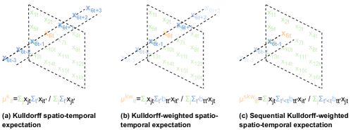
Figure 1: Illustrating the three proposed options to obtain spatio-temporal expectations $\mu_{it}$ used in the computation of SPATE for single-channel data.

For a static, discrete spatial pattern (e.g. a grid of pixels forming an image) consisting of continuous values $x\in\mathbb{R}^{n}$ where $n\in\mathbb{N}$ is the dimensionality of $x$, $x_{i}$ for $i\in 1,\dots,n$ represents the $i$’th pixel value on a regular grid. The local Moran’s I statistic $I_{i}$ is computed as follows:

$$\begin{split}I_{i}=(n_{i}-1)\frac{z_{i}}{\sum^{n_{i}}_{j=1}z_{j}^{2}}\sum^{n_{i}}_{j=1,j\neq i}w_{i,j}z_{j}\end{split}$$ (1)

where $z_{i}=x_{i}-\bar{x}$ is the deviance of observation $x_{i}$ from the global mean $\bar{x}$, $n_{i}$ is the number of spatial neighbors of pixel $x_{i}$, $j$ indexes neighbors of $x_{i}$ for $j\in\{1,...,n_{i}\}$ and $j\neq i$, and $w_{i,j}$ is a binary spatial weight matrix, indicating spatial neighborhood of observations $i$ and $j$. $I_{i}$ can be interpreted as a measure of similarity to neighboring pixels: positive values imply homogeneous clusters, while negative values suggest outliers, change patterns or edges.

Now, let us assume that we observe a sequence of spatial patterns over time $t$: $x=(x_{1},...,x_{T})\in\mathbb{R}^{n\times T}$ where $n$ is the dimensionality of $x_{t}$ at each time $t$ and $T$ is the total time steps of the sequence. Of course, a naive adoption of the approach above is simply to ignore the time component of a sequence and compute the local Moran’s I values $I_{it}$ around pixel $i$ using mean values $\bar{x}_{t}$ at each time $t$. Unfortunately, this approach would strictly separate spatial and temporal effects. In fact, the much more realistic assumption is that space and time are not separable, but do in fact interact and form joint patterns. For this reason, we expand the concept of Moran’s I for spatio-temporal expectations. First, we follow the intuition outlined in Kulldorff et al. (2005) and define expected values of $\mu_{it}(x)$. We refer to this approach as Kulldorff spatio-temporal expectation (”k”):

$$\mu_{it}^{(k)}=\frac{\sum_{j}x_{jt}\sum_{t^{\prime}}x_{it^{\prime}}}{\sum_{j}\sum_{t^{\prime}}x_{jt^{\prime}}}.$$ (2)

$\mu_{it}^{(k)}$ in (2) involves utilizing all spatial units (pixels) available at time step $t$ and across all time steps at a single spatial unit (pixel position) $i$. This computation of the spatio-temporal expectations assumes independence of space and time, and thus the residual $z_{it}=x_{it}-\mu_{it}^{(k)}$ can be thought of as a local measure of space-time interaction at pixel $i$ and time $t$. Moreover, this formulation of $\mu_{it}$ makes two critical assumptions: (1) Different time steps are equally important, irrespective of how distant they are from the current time step. (2) At each time step, we assume availability of the whole time series (i.e. looking into the future is possible). We can modify the computation of $\mu_{it}$ by imposing alternative assumptions.

First, assuming that distant time steps have less significant impact on the current time step, we can integrate temporal weights into the computation, and apply decreasingly lower weights to more distant time steps. For example, one can consider an exponential kernel:

$$\mu_{it}^{(kw)}=\frac{\sum_{j}x_{jt}\sum_{t^{\prime}}b_{tt^{\prime}}x_{it^{\prime}}}{\sum_{j}\sum_{t^{\prime}}b_{tt^{\prime}}x_{jt^{\prime}}},$$ (3)

where $b_{tt^{\prime}}=\exp(-|t-t^{\prime}|/l)$ and $l$ is the lengthscale of the exponential kernel. We refer to this approach as Kulldorff-weighted spatio-temporal expectation (”kw”).

Second, we can restrict the computation of $\mu_{it}$ at time step $t$ to only account for time steps $<t$, so that the expectation at each time step is independent of future observations. Thus, the computation respects the generating logic of sequential data. We refer to this last approach as Kulldorff-sequential-weighted spatio-temporal expectation (”ksw”):

$$\mu_{it}^{(ksw)}=\frac{\sum_{j}x_{jt}\sum_{t^{\prime}<t}b_{tt^{\prime}}x_{it^{\prime}}}{\sum_{j}\sum_{t^{\prime}<t}b_{tt^{\prime}}x_{jt^{\prime}}}.$$ (4)

Note that for the first time step $t=0$, we cannot access past time steps to calculate spatio-temporal expectations $\mu_{i0}^{(ksw)}$.

We can now simply plug in our new spatio-temporal expectations into the Moran’s I metric at time $t$ by replacing spatial only expectations with a spatio-temporal expectation of our choice. As such, we define our novel measure of spatio-temporal association (SPATE),

$$\begin{split}\begin{aligned} S_{it}(x,w)=(n_{i}-1)\frac{z_{it}}{\sum^{n_{x}}_{j=1}z_{jt}^{2}}\sum^{n_{x}}_{j=1,j\neq i}w_{i,j}z_{jt}\end{aligned}\end{split}$$ (5)

where $z_{it}=x_{it}-\mu_{it}$ and $\mu_{it}$ can be any option from $\mu_{it}^{(k)}$, $\mu_{it}^{(kw)}$ and $\mu_{it}^{(ksw)}$. When using $\mu_{it}^{(ksw)}$, SPATE does not return values for $t=0$, as no previous time steps are available to calculate spatio-temporal expectations. See Fig 1 for an illustration of the three proposed options.

SPATE measures spatio-temporal autocorrelation at the input resolution. Its behavior can be closely related to that of the Moran’s I metric. While Moran’s I evaluates the deviance $z_{i}$ between each pixel and the spatial expectation, SPATE does so by using the spatio-temporal expectation $z_{it}$. Like Moran’s I, SPATE acts as a detector of spatio-temporal clusters and change patterns. Like Moran’s I, SPATE identifies positive and negative space-time autocorrelation, i.e. homogeneous areas of similar behavior and outliers that behave differently from their immediate neighborhood. The difference between Moran’s I and SPATE is that the later explicitly captures space-time interactions. For example, if pixel $x_{i}$ and all other data points (not just its neighbors) are increased at a given time step $t$, Moran’s I at time $t$ (for all points) will be high, but SPATE will not be. SPATE of $x_{it}$ will be high if (a) pixel $x_{it}$ is high compared to its expectation at the same time $t$, (b) its neighbors are high compared to their expectations, while (c) its non-neighbors are not particularly high compared to their expectations.

In the $kw$ and $ksw$ settings, the lengthscale parameter $l$ governs whether the metric captures longer or shorter term temporal patterns. For example, if pixel $x_{it}$ and its neighbors increase slowly over time, that change will only cause SPATE to be high for larger lengthscales $l$, while smaller $l$ values imply that current values are compared to those that are close in time. As such, the lengthscale determines what changes are considered ”slow” (incorporated into the mean, not detected as space-time interaction) and ”fast” (current values are different from the mean, detected as space-time interaction). The $ksw$ setting further allows for scenarios where we might wish to compute the metric based on previous time-steps alone, i.e. to preserve sequential logic.

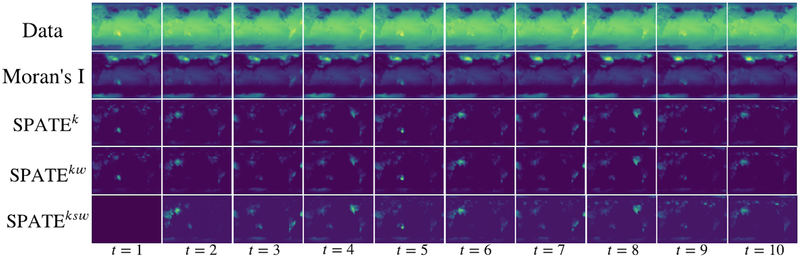
Figure 2: The SPATE metric in its different forms computed for an example from the LGCP datasets. While $\text{SPATE}^{k}$ and $\text{SPATE}^{kw}$ are visually undistinguishable, $\text{SPATE}^{ksw}$ changes as increasingly more past time steps become available, converging to $\text{SPATE}^{kw}$ at time $T$. We can also observe how the Moran’s I metric remains static in time, while all versions of SPATE behave dynamically in space and time.

COT-GAN

Built upon the theory of Causal Optimal Transport (COT), COT-GAN was introduced by Xu et al. (2020) as an adversarial algorithm to train implicit generative models for sequential learning. COT can be considered as a maximization over the classical (Kantorovich) optimal transport (OT) with a temporal causality constraint, which restricts the transporting of mass on the arrival sequence at any time $t$ to depend on the starting sequence only up to time $t$. This motivated us to design the spatio-temporal expectation $\mu_{it}^{ksw}$ in order to respect the nature of sequential data that are generated in an autoregressive manner.

In sequential generation, we are interested in learning a model that produces $y=(y_{1},...,y_{T})\in\mathbb{R}^{n\times T}$ to mimic $x=(x_{1},...,x_{T})\in\mathbb{R}^{n\times T}$. Given two probability measures $\mu,\nu$ defined on $\mathbb{R}^{n\times T}$, and a cost function $c:\mathbb{R}^{n\times T}\times\mathbb{R}^{n\times T}\to\mathbb{R}$, the causal optimal transport of $\mu$ into $\nu$ is formulated as

$$\mathcal{W}^{\mathcal{K}}_{c}(\mu,\nu):=\inf_{\pi\in\Pi^{\mathcal{K}}(\mu,\nu)}\mathbb{E}^{\pi}[c(x,y)],$$ (6)

where $\Pi^{\mathcal{K}}(\mu,\nu)$ is the set of probability measures $\pi$ on $\mathbb{R}^{n\times T}\times\mathbb{R}^{n\times T}$ with marginals $\mu,\nu$, which also satisfy the constraint

$$\pi(dy_{t}|dx_{1:T})=\pi(dy_{t}|dx_{1:t})\quad\text{for all\, $t=1,\cdots,T-1$}.$$

Such plans in $\Pi^{\mathcal{K}}(\mu,\nu)$ are called causal transport plans. Here $c(x,y)$ is a cost function that measures the loss incurred by transporting a unit of mass from $x$ to $y$. $\mathcal{W}^{\mathcal{K}}_{c}(\mu,\nu)$ is thus the minimal total cost for moving the mass $\mu$ to $\nu$ in a causal way.

In comparison, the (classic) OT is defined on $\mathbb{R}^{n}$ and differs from COT by searching an optimal plan that leads to the least cost in a less restricted space $\Pi(\mu,\nu)$ which contains all transport plans,

$$\mathcal{W}_{c}(\mu,\nu):=\inf_{\pi\in\Pi(\mu,\nu)}\mathbb{E}^{\pi}[c(x,y)].$$ (7)

COT-GAN constructed an adversarial objective by reformulating the COT (6) as below,

$$\mathcal{W}^{\mathcal{K}}_{c}(\mu,\nu)=\sup_{c^{\mathcal{K}}\in\mathcal{C}^{\mathcal{K}}(\mu,c)}\inf_{\pi\in\Pi(\mu,\nu)}\{\mathbb{E}^{\pi}[c^{\mathcal{K}}(x,y)]\},$$ (8)

where $\mathcal{C}^{\mathcal{K}}(\mu,c)$ is a special family of costs that encode the causality constraint, see Appendix A for details. Note that the inner optimization problem is equivalent to OT in (7) with a specific class of cost function, i.e., $\mathcal{W}_{c^{\mathcal{K}}}(\mu,\nu)=\inf_{\pi\in\Pi(\mu,\nu)}\{\mathbb{E}^{\pi}[c^{\mathcal{K}}(x,y)]\}$.

In the implementation of COT-GAN, learning is done via stochastic gradient descent (SGD) on mini-batches. Given a distribution $\zeta$ on some latent space $\mathcal{Z}$, the generator $g_{\theta}$ is a function that maps a latent variable $z\sim\zeta$ to the generated sequence $y$ in the path space. Given a mini-batch of size $m$ from training data $\{x^{d}_{1:T}\}_{i=1}^{m}$ and that from generated samples $\{y^{d}_{1:T}\}_{i=1}^{m}$, we define the empirical measures for the mini-batches as

$$\hat{\mu}:=\frac{1}{m}\sum_{d=1}^{m}\delta_{{x}^{d}_{1:T}},\quad\hat{\nu}_{\theta}:=\frac{1}{m}\sum_{d=1}^{m}\delta_{{y}^{d}_{1:T}},$$

where $\hat{\nu}_{\theta}$ incorporates the parameterization of $g_{\theta}$. Thus, the duality of COT given by (8) between the empirical measures of two mini-batches can be written as

$$\mathcal{W}^{\mathcal{K}}_{c}(\hat{\mu},\hat{\nu}_{\theta})=\sup_{c^{\mathcal{K}}\in\mathcal{C}^{\mathcal{K}}(\hat{\mu},c)}\mathcal{W}_{c^{\mathcal{K}}}(\hat{\mu},\hat{\nu}_{\theta}).$$ (9)

Computing (9) involves solving the optimization problem of classic OT. COT-GAN opted for the Sinkhorn algorithm, see (Cuturi 2013; Genevay, Peyre, and Cuturi 2018), and a modified version of Sinkhorn divergence for an approximation. Here we have the entropic-regularized OT defined as

$$\mathcal{W}_{c,\varepsilon}(\mu,\nu):=\inf_{\pi\in\Pi(\mu,\nu)}\{\mathbb{E}^{\pi}[c(x,y)]-\varepsilon H(\pi)\},\quad\varepsilon>0,$$

where $H(\pi)$ is the Shannon entropy of $\pi$. Whilst the Sinkhorn divergence was also computed between two mini-batches, the authors of COT-GAN noticed the bias was better reduced by the mixed Sinkhorn divergence,

$$\widehat{\mathcal{W}}_{c,\varepsilon}^{\text{mix}}(\hat{\mu},\hat{\nu},\hat{\mu}^{\prime},\hat{\nu}^{\prime}) :=\mathcal{W}_{c,\varepsilon}(\hat{\mu},\hat{\nu})+\mathcal{W}_{c,\varepsilon}(\hat{\mu}^{\prime},\hat{\nu}^{\prime})$$

$$\quad-\mathcal{W}_{c,\varepsilon}(\hat{\mu},\hat{\mu}^{\prime})-\mathcal{W}_{c,\varepsilon}(\hat{\nu},\hat{\nu}^{\prime}),$$

where $\hat{\mu}$ and $\hat{\mu}^{\prime}$ represent the empirical measures corresponding to two different mini-batches of the training data, and $\hat{\nu}$ and $\hat{\nu}^{\prime}$ are the ones to the generated samples.

Finally, we have the following objective function for COT-GAN:

$$\inf_{\theta}\sup_{\varphi}\bigg{\{}\widehat{\mathcal{W}}_{c^{\mathcal{K}}_{\varphi},\varepsilon}^{\text{mix}}(\hat{\mu},\hat{\nu}_{\theta},\hat{\mu}^{\prime},\hat{\nu}^{\prime}_{\theta})-\lambda\big{[}p_{{\bf M}_{\varphi_{2}}}(\hat{\mu})+p_{{\bf M}_{\varphi_{2}}}(\hat{\mu}^{\prime})\big{]}\bigg{\}},$$

where the role of discriminator is played by the cost function $c^{\mathcal{K}}$ parameterized by $\varphi$, and $p_{{\bf M}_{\varphi_{2}}}$ is the martingale penalization required for the formulation of the new class of costs $\mathcal{C}^{\mathcal{K}}_{\varphi}$, and $\varphi_{2}$ is a subset of the discriminator parameters $\varphi$, see details in Appendix A. Similar to common GAN training scheme, the discriminator learns the worst-case cost $c^{\mathcal{K}}_{\varphi}$ by maximizing the objective over $\varphi$, and the generator is updated by minimizing it over $\theta$.

SPATE-GAN

In SPATE-GAN, we integrate our newly devised spatio-temporal metric into the COT-GAN objective function. We compute the embedding for each $x^{d}_{it}$ and $y^{d}_{it}$ in minibatches $\{x^{d}_{1:T}\}_{d=1}^{m}$ and $\{y^{d}_{1:T}\}_{d=1}^{m}$ by

$$\hat{x}^{d}_{it}=S_{it}(x^{d}_{1:T},w)\quad\text{and}\quad\hat{y}^{d}_{it}=S_{it}(y^{d}_{1:T},w),$$

where the binary spatial weight matrix $w$ is pre-defined.

The corresponding embeddings are then concatenated with the training data and generated samples on the channel dimension. We define the empirical measures for the concatenated sequences as

$$\widehat{\mu}^{e}:=\frac{1}{m}\sum_{d=1}^{m}\delta_{\text{concat}({x}^{d}_{1:T},\hat{x}_{1:T}^{d}))},$$

$$\widehat{\nu}^{e}_{\theta}:=\frac{1}{m}\sum_{d=1}^{m}\delta_{\text{concat}({y}^{d}_{1:T},\hat{y}_{1:T}^{d})},$$

where $\text{concat}(.,.)$ is an operator that concatenates inputs along the channel dimension.

We thus arrive at the objective function for SPATE-GAN:

$$\inf_{\theta}\sup_{\varphi} \bigg{\{}\widehat{\mathcal{W}}_{c^{\mathcal{K}}_{\varphi},\varepsilon}^{\text{mix}}(\widehat{\mu}^{e},\widehat{\nu}^{e}_{\theta},\widehat{\mu}^{e^{\prime}},\widehat{\nu}^{e^{\prime}}_{\theta})$$

$$\quad-\lambda\big{[}p_{{\bf M}_{\varphi_{2}}}(\widehat{\mu}^{e})+p_{{\bf M}_{\varphi_{2}}}(\widehat{\mu}^{e^{\prime}})\big{]}\bigg{\}}.$$

We maximize the objective function over $\varphi$ to search for a worst-case distance between the two empirical measures, and minimize it over $\theta$ to learn a distribution that is as close as possible to the real distribution. The algorithm is summarized in Algorithm 1. Its time complexity scales as $\mathcal{O}((J+2n)LTm^{2})$ in each iteration where $J$ is the output dimension of the discriminator (see Appendix A for details), and $L$ is the number of Sinkhorn iterations (see Genevay, Peyre, and Cuturi (2018); Cuturi (2013) for details).

In the experiment section, we will compare SPATE-GAN with three different expectations $\mu_{it}^{(k)}$, $\mu_{it}^{(kw)}$ and $\mu_{it}^{(ksw)}$ in the computation of SPATE. Hence, we denote the corresponding models as $\text{SPATE-GAN}^{k}$, $\text{SPATE-GAN}^{kw}$, and $\text{SPATE-GAN}^{ksw}$, respectively.

Last, we would like to emphasize that, although all three embeddings consider the space-time interactions in a certain way, the non-anticipative assumption of $\mu_{it}^{(ksw)}$ is consistent with the generating process of the type of data we are investigating. As the causality constraint in COT-GAN also restricts the search of transport plans to those that satisfy non-anticipative transporting of mass, $\text{SPATE-GAN}^{ksw}$ is a model that fully respects temporal causality in learning, whilst $\text{SPATE-GAN}^{k}$ and $\text{SPATE-GAN}^{kw}$ also combine information from the future.

Data: $\{{x}^{d}_{1:T}\}_{d=1}^{n}$ (input data), $\zeta$ (latent distribution)

Parameters: $\theta_{0}$, $\varphi_{0}$ (parameter initializations), $m$ (batch size), $\varepsilon$ (regularization parameter), $\alpha$ (learning rate), $\lambda$ (martingale penalty coefficient)

Initialize: $\theta\leftarrow\theta_{0}$, $\varphi\leftarrow\varphi_{0}$

for $b=1,2,\dots$ do

        Sample $\{{x}^{d}_{1:T}\}_{d=1}^{m}$ from real data;

      [0.1cm]  Sample $\{{z}^{d}_{1:T}\}_{d=1}^{m}$ from  $\zeta$;

      [0.1cm]  Generate sequences from latent: $(y_{1:T}^{d})\leftarrow g_{\theta}({z}^{d}_{1:T})$;

      [0.1cm]  Compute the embeddings: $\hat{x}^{d}_{it}=S_{it}(x^{d}_{1:T},w),\quad\hat{y}^{i}_{it}=S_{it}(y^{i}_{1:T},w)$;

      [0.1cm]  Concatenated the data with embeddings: $\text{concat}({x}^{d}_{1:T},\hat{x}_{1:T}^{d}),\text{concat}({y}^{d}_{1:T},\hat{y}_{1:T}^{d})$ ;

      [0.1cm]  Update discriminator parameter:

       [0.1cm] ${\varphi}\leftarrow{\varphi}+\alpha\nabla_{\varphi}\big{(}\widehat{\mathcal{W}}_{c^{\mathcal{K}}_{\varphi},\varepsilon}^{\text{mix}}(\widehat{\mu}^{e},\widehat{\nu}^{e}_{\theta},\widehat{\mu}^{e^{\prime}},\widehat{\nu}^{e^{\prime}}_{\theta})-\lambda\big{[}p_{{\bf M}_{\varphi_{2}}}(\widehat{\mu}^{e})+p_{{\bf M}_{\varphi_{2}}}(\widehat{\mu}^{e^{\prime}})\big{]}\big{)}$;

      [0.1cm]  Sample $\{{z}^{d}_{1:T}\}_{d=1}^{m}$ from $\zeta$;

      [0.1cm]  Generate sequences from latent: $(y_{1:T}^{d})\leftarrow g_{\theta}({z}^{d}_{1:T})$;

      [0.1cm]  Compute the embeddings: $\hat{x}^{d}_{it}=S_{it}(x^{d}_{1:T},w),\quad\hat{y}^{d}_{it}=S_{it}(y^{d}_{1:T},w)$;

      [0.1cm]  Concatenated the data with embeddings: $\text{concat}({x}^{d}_{1:T},\hat{x}_{1:T}^{d}),\text{concat}({y}^{d}_{1:T},\hat{y}_{1:T}^{d})$ ;

      [0.1cm]  Update generator parameter: $\theta\leftarrow\theta-\alpha\nabla_{\theta}\left(\widehat{\mathcal{W}}_{c^{\mathcal{K}}_{\varphi},\varepsilon}^{\text{mix}}(\widehat{\mu}^{e},\widehat{\nu}^{e}_{\theta},\widehat{\mu}^{e^{\prime}},\widehat{\nu}^{e^{\prime}}_{\theta})\right)$;

end for

Algorithm 1 training SPATE-GAN by SGD

Experiments

To empirically evaluate SPATE-GAN, we use three datasets characterized by different spatio-temporal complexities.

Extreme Weather (EW)

This dataset, introduced by Racah et al. (2017), was originally proposed for detecting extreme weather events from a range of climate variables (e.g. zonal winds, radiation). Each of these climate variables is observed four times a day for a $128\times 192$ pixel representation of the whole earth. We chose to model surface temperatureas it comes with several interesting spatio-temporal characteristics: It exhibits both static (e.g. continent outlines) and dynamic patterns as well as abnormal patterns (e.g. in the presence of tropical cyclones or atmospheric rivers). Furthermore, simulating climate data is an important potential downstream application of deep generative models.

LGCP

This dataset represents the intensities (number of events in a grid cell) of a log-Gaussian Cox process (LGCP), a continuous spatio-temporal point process. LGCPs are a popular class of models for simulating contagious spatio-temporal patterns and have various applications, for example in epidemiology. We simulate $300$ different LGCP intensities on a $64\times 64$ grid over $10$ time steps using the R package LGCP (Taylor et al. 2015).

Turbulent Flows (TF)

This dataset, proposed by (Wang et al. 2020b), simulates velocity fields according to the Navier-Stokes equation. This is a class of partial differential equations describing the motion of fluids. Fluid dynamics and simulation is another potential application of deep generative models. Following the approach of Wang et al. (2020b), we divide the data into $7$ steps of $64\times 64$ pixel frames. Please note that we only utilize the first velocity field, so that all our utilized datasets are single-channel.

Baselines and evaluation metrics

We use COT-GAN (Xu et al. 2020) and GAN proposed by (Genevay, Peyre, and Cuturi 2018), which we name as SinkGAN, as base models. We augment both models with our new embedding loss, using SPATE with $k$, $kw$ and $ksw$ configurations. We refer to all models using a COT-GAN backbone in combination with our new embedding loss as SPATE-GAN. We further denote the SinkGAN models corresponding to three SPATE settings as $\text{SinkGAN}^{k}$, $\text{SinkGAN}^{kw}$ and $\text{SinkGAN}^{ksw}$. To compare our approach to a non-time-sensitive embedding, we also deploy models using the Moran’s I metric using the same embedding loss procedure, denoted as $\text{COT-GAN}^{M}$ and $\text{SinkGAN}^{M}$.

To compare our GAN output to real data samples, we use three different metrics: Earth Mover Distance (EMD), Maximum Mean Discrepancy (MMD) (Borgwardt et al. 2006) and a classifier two-sample test based on a k-nearest-neighbor (KNN) classifier with $k=1$ (Lopez-Paz and Oquab 2019). All these measures are general purpose GAN metrics. While GAN metrics specialized on video data exist, they rely on extracting features from models pre-trained on three-channel RGB video data. As we are working with single-channel, non-image data, these methods are not applicable in our case.

Experimental Setting

We compare SPATE-GAN to a range of baseline configurations. We use the same GAN architecture for all these settings to ensure comparability. Our GAN generators feed the noise input through two LSTM layers to obtain time-dependent features. These are then mapped into the desired shape for deconvolutional operations using a fully-connected layer with a leaky ReLU activation. Lastly, 4 deconvolutional layers map the output into video frames, all also with leaky ReLU activations. Our discriminators initially feed video input through three convolutional layers with leaky ReLU activations. The outputs from the convolutional operations are then reshaped and fed through two LSTM layers to create the final discriminator outputs.

All our models are implemented in PyTorch (Paszke et al. 2019) and optimized using the Adam algorithm (Kingma and Ba 2015). Our experiments are conducted on a single Geforce 1080Ti or RTX 3090 GPU. Further training details can be found in Appendix B.

Results

Results from our experiments are shown in Table 1. Visual comparisons between real and generated data from the different models are shown in Figures 3,4, and 5. For larger figures including results from all tested model configurations, please see the Appendix D. Through all experiments we can observe that $\text{SPATE-GAN}^{ksw}$ consistently outperforms the competing approaches, achieving the best scores across all datasets and evaluation metrics.

Table 1: Evaluations for LGCP, EW and TF datasets. Lower values in EMD and MMD indicate better sample quality, while values close to 0.5 are more desirable for KNN.

LGCP	EMD	MMD	KNN
SinkGAN	12.46 (0.02)	0.38 (0.001)	0.14 (0.001)
$\text{SinkGAN}^{M}$	12.46 (0.02)	0.38 (0.001)	0.14 (0.001)
$\text{SinkGAN}^{k}$	12.65 (0.03)	0.38 (0.001)	0.15 (0.001)
$\text{SinkGAN}^{kw}$	10.60 (0.01)	0.63 (0.008)	0.30 (0.002)
$\text{SinkGAN}^{ksw}$	13.33 (0.01)	0.36 (0.001)	0.38 (0.003)
COT-GAN	12.38 (0.02)	0.30 (0.001)	0.20 (0.004)
$\text{COT-GAN}^{M}$	12.38 (0.02)	0.30 (0.001)	0.20 (0.004)
$\text{SPATE-GAN}^{k}$	11.56 (0.02)	0.32 (0.01)	0.31 (0.01)
$\text{SPATE-GAN}^{kw}$	10.92 (0.03)	0.64 (0.035)	0.15 (0.006)
$\text{SPATE-GAN}^{ksw}$	10.47 (0.02)	0.30 (0.001)	0.39 (0.01)
Extreme Weather
SinkGAN	29.40 (0.05)	0.49 (0.001)	0.41 (0.004)
$\text{SinkGAN}^{M}$	29.27 (0.05)	0.72 (0.002)	0.22 (0.01)
$\text{SinkGAN}^{k}$	32.57 (0.03)	0.81 (0.001)	0.16 (0.004)
$\text{SinkGAN}^{kw}$	32.78 (0.05)	0.81 (0.001)	0.18 (0.004)
$\text{SinkGAN}^{ksw}$	30.00 (0.04)	0.50 (0.001)	0.41 (0.004)
COT-GAN	26.66 (0.09)	0.43 (0.002)	0.42 (0.002)
$\text{COT-GAN}^{M}$	36.42 (0.14)	0.65 (0.002)	0.09 (0.01)
$\text{SPATE-GAN}^{k}$	33.58 (0.07)	0.73 (0.002)	0.15 (0.01)
$\text{SPATE-GAN}^{kw}$	33.36 (0.09)	0.72 (0.002)	0.13 (0.003)
$\text{SPATE-GAN}^{ksw}$	26.24 (0.07)	0.42 (0.002)	0.42 (0.002)
Turbulent Flows
SinkGAN	26.52 (0.007)	1.23 (0.001)	0.15 (0.001)
$\text{SinkGAN}^{M}$	28.02 (0.005)	1.22 (0.0002)	0.01 (0.002)
$\text{SinkGAN}^{k}$	28.14 (0.002)	1.32 (0.002)	0.08 (0.001)
$\text{SinkGAN}^{kw}$	30.98 (0.001)	1.50 (0.001)	0.03 (0.001)
$\text{SinkGAN}^{ksw}$	25.47 (0.008)	1.24 (0.0002)	0.13 (0.002)
COT-GAN	27.03 (0.01)	1.22 (0.001)	0.16 (0.002)
$\text{COT-GAN}^{M}$	24.93 (0.01)	1.19 (0.001)	0.09 (0.002)
$\text{SPATE-GAN}^{k}$	25.70 (0.02)	1.21 (0.001)	0.12 (0.003)
$\text{SPATE-GAN}^{kw}$	24.30 (0.002)	1.42 (0.001)	0.13 (0.004)
$\text{SPATE-GAN}^{ksw}$	22.98 (0.01)	1.16 (0.001)	0.16 (0.002)

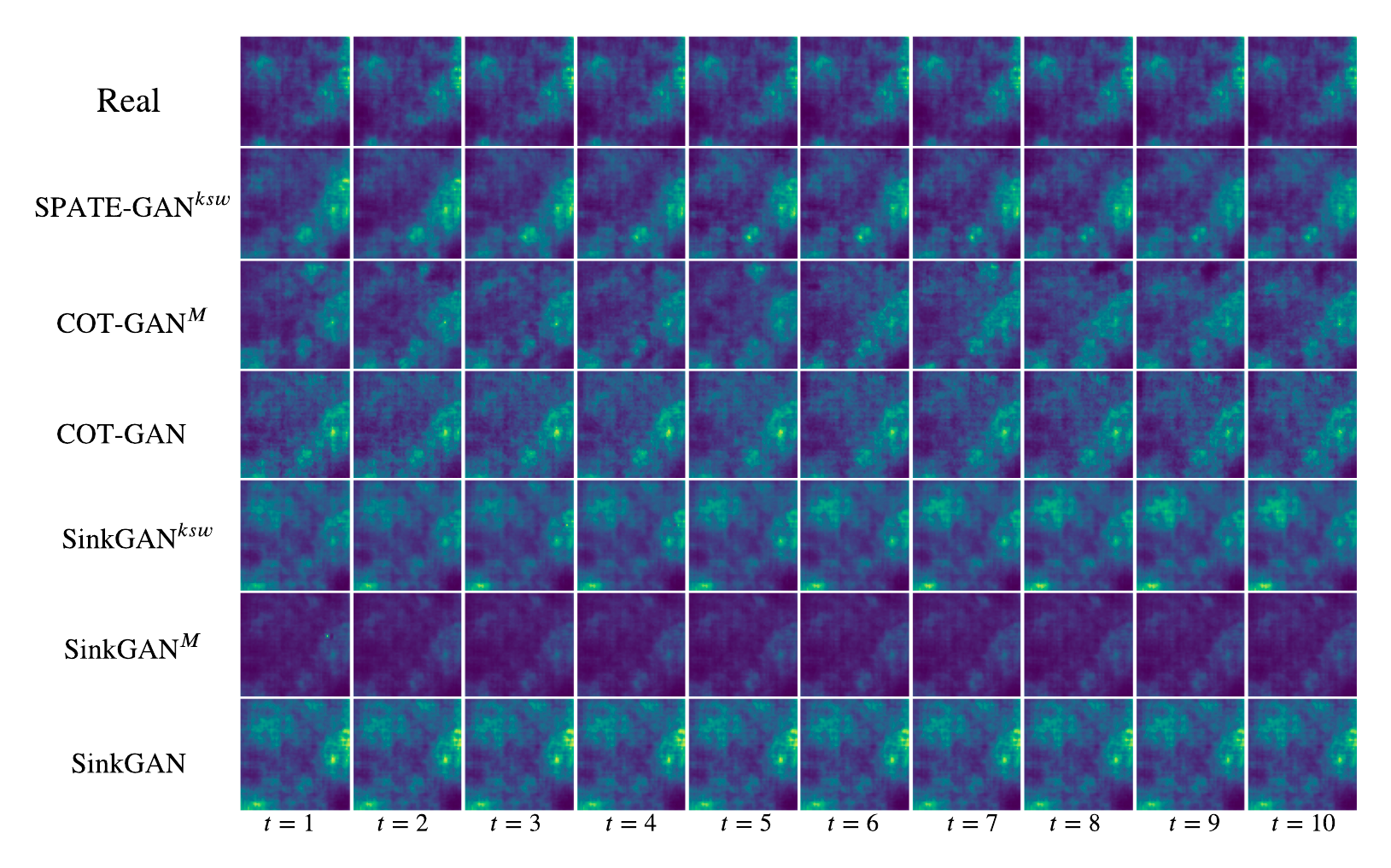
Figure 3: Selected samples for LGCP dataset.

This finding is interesting as the $ksw$ setting theoretically looses information over the $k$ and $kw$ approaches, which both have access to future time steps when calculating the SPATE metric. Nevertheless, this result underlines the strong synergies between $\text{SPATE}^{ksw}$ and the COT-GAN backbone: The metric is calculated in sequential fashion and thus respects the same causality constraints that restrict COT-GAN. As such, the outcome, while noteworthy, is not surprising.

This result is strengthened by a comparison with the SinkGAN-based approaches: SinkGAN does not follow the same restrictions and, as we observe, is not improved as consistently by the SPATE-based embedding losses. In fact, in some cases the naive SinkGAN performs better than its derivatives using SPATE or Moran’s I based embedding losses.

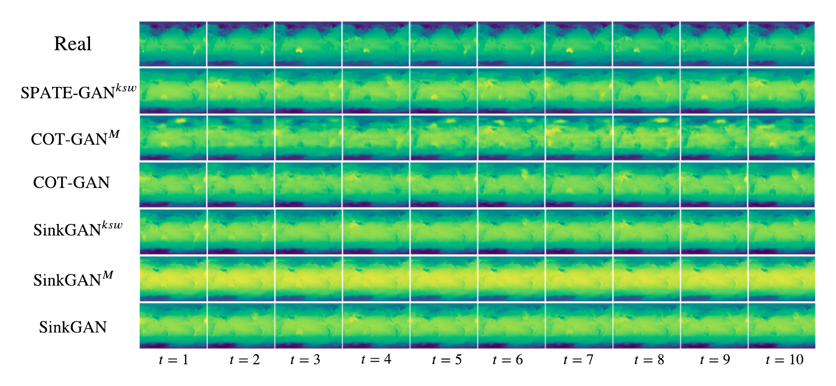
Figure 4: Selected samples for Extreme Weather dataset.

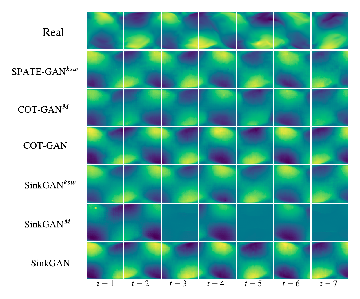
Figure 5: Selected samples for Turbulent Flows dataset.

We also observe that throughout all settings, models using Moran’s I perform similarly to their naive counterparts. This confirms that in fact, simply using measures of spatial autocorrelation computed over a sequence is not sufficient for capturing complex spatio-temporal effects. On the contrary, the other two SPATE settings, $k$ and $kw$, both appear to have beneficial effects and improve performance.

In summary, our results highlight how COT-GAN combined with a non-anticipative measure of space-time association can improve the modeling of complex spatio-temporal patterns. This finding represents another step on the way towards deep learning methods specialized on the dynamics driving many systems on our planet.

Furthermore, we provide an investigation on the impact of the lengthscale parameter $l$ in the spatio-temporal expectations for $l\in\{1,10,20,30,50\}$. As shown in Figure 6, $l=20$ leads to better EMD and KNN results whilst all MMD scores remain unchanged. For the results presented in this paper, we set $l=20$ in all our experiments.

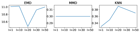
Figure 6: Evaluations of $\text{SPATE-GAN}^{ksw}$ (left: EMD, middle: MMD, and right: KNN) on LGCP dataset given lengthscale $l\in\{1,10,20,30,50\}$.

Conclusion

Recent studies have called for more research into improving deep learning models for spatio-temporal earth systems data (Reichstein et al. 2019). Other academic domains have dealt with these data for many decades and have developed methods for capturing specific spatial and spatio-temporal effects. Inspired by their approaches, we devise SPATE, a measure of spatio-temporal association capable of detecting emerging space-time clusters and homogeneous areas in the data. We then develop a novel embedding loss for video GANs utilizing SPATE as a means of reinforcing the learning of these patterns-of-interest. Our new generative modeling approach, SPATE-GAN, shows performance increases on a range of different datasets emulating the real-world complexities of spatio-temporal dynamics. As such, this study highlights how domain expertise from applied academic areas can help to motivate methodological advances in machine learning.

Appendix

A: Details for COT-GAN

The family of cost functions $\mathcal{C}^{\mathcal{K}}(\mu,c)$ is given by

$$\mathcal{C}^{\mathcal{K}}(\mu,c):=\Bigg{\{} c(x,y)+\sum_{j=1}^{J}\sum_{t=1}^{T-1}h^{j}_{t}(y)\Delta_{t+1}M^{j}(x):$$

$$J\in\mathbb{N},(h^{j},M^{j})\in\mathcal{H}(\mu)\Bigg{\}},$$

where $\Delta_{t+1}M(x):=M_{t+1}(x_{1:t+1})-M_{t}(x_{1:t})$ and $\mathcal{H}(\mu)$ is a set of functions depicting causality:

$$\mathcal{H}(\mu):=\{ (h,M):h=(h_{t})_{t=1}^{T-1},\ h_{t}\in\mathcal{C}_{b}(\mathbb{R}^{n\times t}),$$

$$M=(M_{t})_{t=1}^{T}\in\mathcal{M}(\mu),M_{t}\in\mathcal{C}_{b}(\mathbb{R}^{n\times t})\},$$

with $\mathcal{M}(\mu)$ being the set of martingales on $\mathbb{R}^{n\times T}$ w.r.t. the canonical filtration and the measure $\mu$, and $\mathcal{C}_{b}(\mathbb{R}^{n\times t})$ the space of continuous, bounded functions on $\mathbb{R}^{n\times t}$.

Moreover, in the implementation of COT-GAN, the dimensionality of the sets of $\mathbf{h}:=(h^{j})_{j=1}^{J}$ and $\mathbf{M}:=(M^{j})_{j=1}^{J}$ is bounded by a fixed $J\in\mathbb{N}$. The discriminator in COT-GAN is formulated by parameterizing $\mathbf{h}_{\varphi_{1}}$ and $\mathbf{M}_{\varphi_{2}}$ in the cost function $c^{\mathcal{K}}$ as two separate neural networks that respect causality,

$$c^{\mathcal{K}}_{\varphi}(x,y)=c(x,y)+\sum_{j=1}^{J}\sum_{t=1}^{T-1}h^{j}_{\varphi_{1},t}(y)\Delta_{t+1}M^{j}_{\varphi_{2}}(x),$$ (10)

where $\varphi:=(\varphi_{1},\varphi_{2})$ and $J$ corresponds to the output dimensionality of the two networks. Thus, we update the parameters based upon the loss given by (8) between the empirical distributions of two mini-batches,

Given a mini-batch of size $m$ from training data $\{x^{d}_{1:T}\}_{i=1}^{m}$ we define the empirical measure for the mini-batch as

$$\hat{\mu}:=\frac{1}{m}\sum_{d=1}^{m}\delta_{{x}^{d}_{1:T}}.$$

As the last piece of the puzzle, Xu et al. (2020) enforced $\mathbf{M}$ to be close to a martingale by a regularization term to penalize deviations from being a martingale on the level of mini-batches.

$${p}_{\mathbf{M}}(\widehat{\mu}):=\frac{1}{mT}\sum_{j=1}^{J}\sum_{t=1}^{T-1}\Bigg{|}\sum_{d=1}^{m}\frac{M^{j}_{t+1}(x^{d}_{1:t+1})-M^{j}_{t}(x^{d}_{1:t})}{\sqrt{\text{Var}[M^{j}]}+\eta}\Bigg{|},$$

where $\text{Var}[M]$ is the empirical variance of $M$ over time and batch, and $\eta>0$ is a small constant.

B: Training details

Table 2: Generator architecture.

Generator	Configuration
Input	$z\sim\mathcal{N}(\mathbf{0},\mathbf{I})$
0	LSTM(state size = 64), BN
1	LSTM(state size = 128), BN
2	Dense(8*8*256), BN, LeakyReLU
3	reshape to 4D array of shape (m, 8, 8, 256)
4	DCONV(N256, K5, S1, P=SAME), BN, LeakyReLU
5	DCONV(N128, K5, S2, P=SAME), BN, LeakyReLU
6	DCONV(N64, K5, S2, P=SAME), BN, LeakyReLU
7	DCONV(N1, K5, S2, P=SAME)

Table 3: Discriminator architecture.

Discriminator	Configuration
Input
0	CONV(N64, K5, S2, P=SAME), BN, LeakyReLU
1	CONV(N128, K5, S2, P=SAME), BN, LeakyReLU
2	CONV(N256, K5, S2, P=SAME), BN, LeakyReLU
3	reshape to 3D array of shape (m, T, -1)
4	LSTM(state size = 256), BN
5	LSTM(state size = 64)

We used a smaller size of model with the same network architectures as COT-GAN to train all three datasets. The architectures for generator and discriminator are given in Tables 2 and 3.

Hyperparameter settings are as follows: the Sinkhorn regularizer $\epsilon=0.8$, Sinkhorn iteration $L=100$, the lengthscale $l=20$ and martingale penalty $\lambda=1.5$. We used Adam optimizer with learning rate $0.0001$, $\beta_{1}=0.5$ and $\beta_{2}=0.9$. All models are trained for $60,000$ iterations.

C: Evaluation metrics

To compute our three metrics, let us first assume that we have a set of real data samples ($\mathcal{P}$) and synthetic data samples ($\mathcal{S}$). EMD is defined as:

$$EMD(\mathcal{P},\mathcal{S})=\min_{\phi:\mathcal{P}\rightarrow\mathcal{S}}\sum_{p\in\mathcal{P}}\|p-\phi(p)\|$$ (11)

where $\phi:\mathcal{P}\rightarrow\mathcal{S}$ is a bijection. MMD is defined as:

$$\widehat{MMD}^{2}(\mathcal{P},\mathcal{S})=\frac{1}{n(n-1)}\sum k(p,p)+$$ (12)

$$\frac{1}{n(n-1)}\sum k(s,s)-\frac{2}{n^{2}}\sum k(p,s)$$

where $k$ denotes a positive-definite kernel (e.g. RBF kernel) and $n$ is the number of (real or synthetic) samples.

Lastly, to compute the KNN score, we first split our real and synthetic samples $\mathcal{P}$ and $\mathcal{S}$ into training and test datasets $\mathcal{D}_{tr}$ and $\mathcal{D}_{te}$ so that $\mathcal{D}=\mathcal{D}_{tr}\cup\mathcal{D}_{te}$. We train the KNN classifier $f:\mathcal{X}_{tr}\rightarrow[0,1]$ using training data. The accuracy of the trained classifier is then obtained using test samples $\mathcal{D}_{te}$ and given as:

$$\hat{t}=\frac{1}{n_{te}}\sum_{(z_{i},l_{i})\in\mathcal{D}_{te}}\mathbb{I}\left[\left(f(z_{i})>\frac{1}{2}\right)=l_{i}\right]$$ (13)

where $f(z_{i})$ estimates the conditional probability distribution $p(l=1|z_{i})$. A classifier accuracy approaching random chance (50%) indicates better synthetic data. As suggested by Lopez-Paz and Oquab (2019), we use a $1$-NN classifier to obtain the score.

D: More figures

In this section, we provide more results in larger figures for visual comparisons.

Figure 7: Larger version of Figure 2 for the purpose of visual comparison.

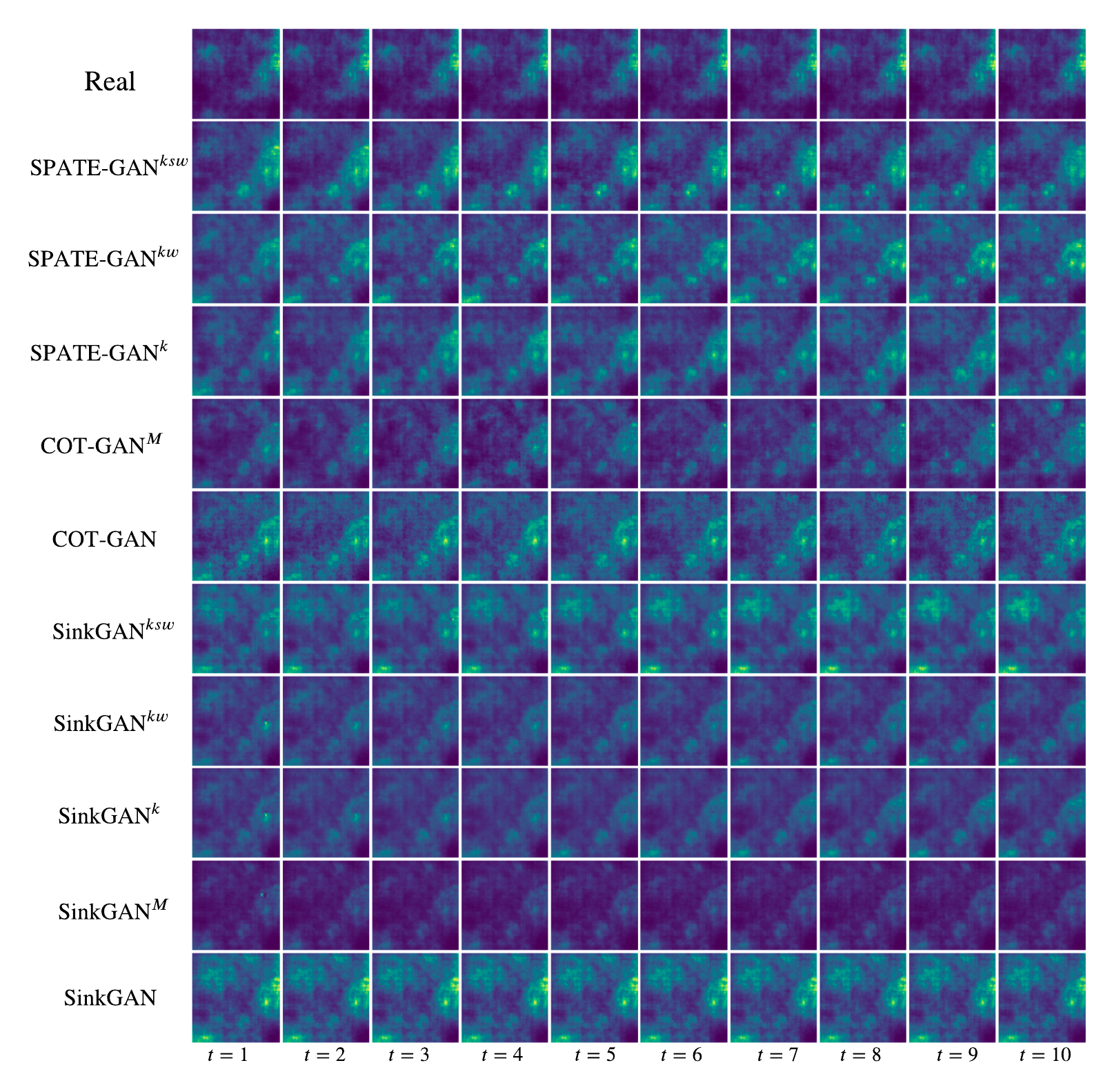
Figure 8: More selected samples for log-Gaussian Cox process (LGCP) dataset.

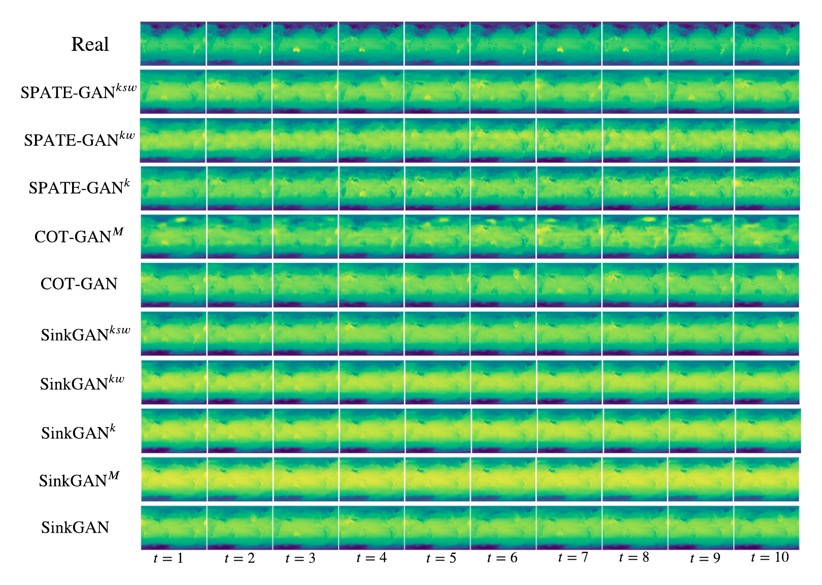
Figure 9: More selected samples for extreme weather (EW) dataset.

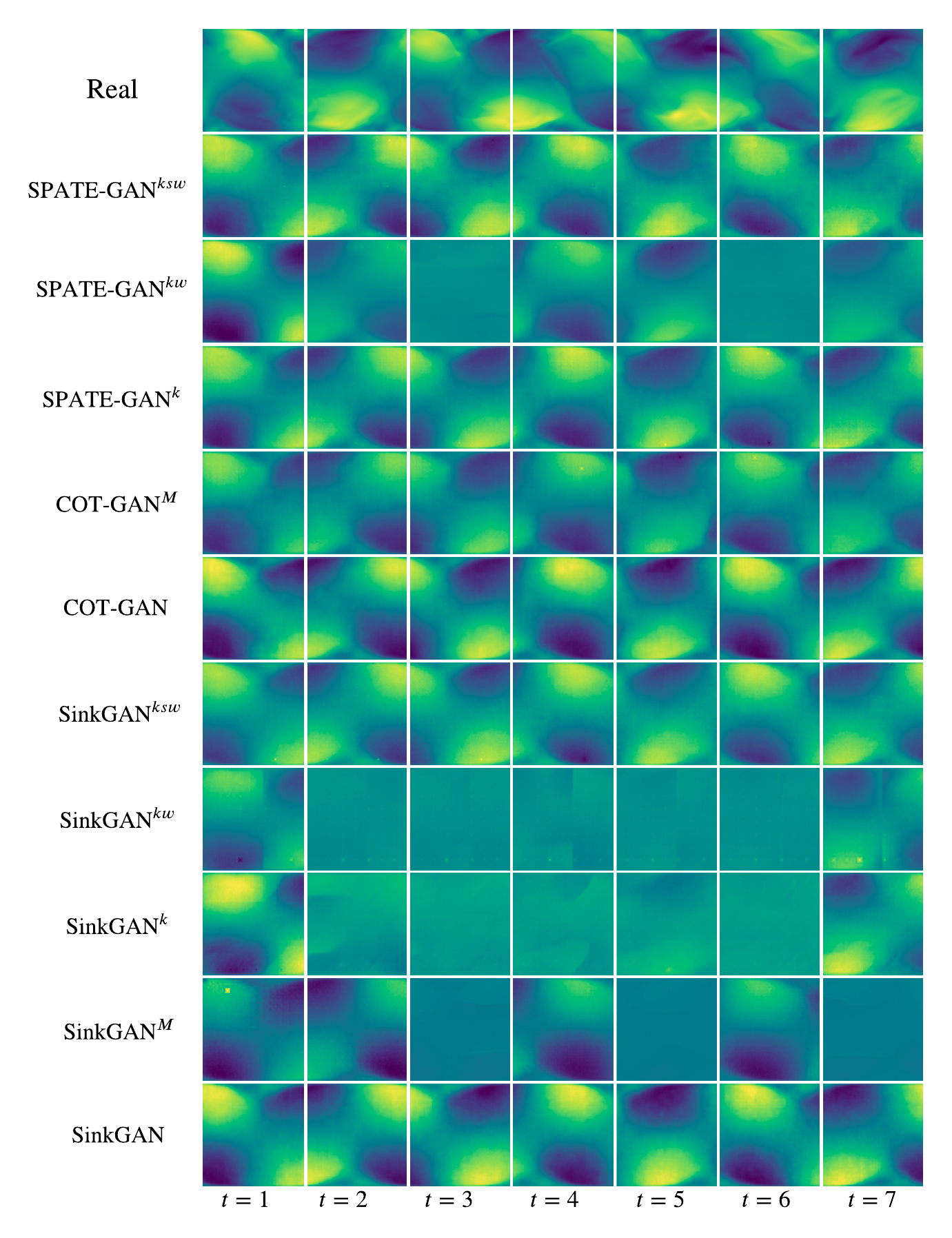
Figure 10: More selected samples for turbulent flow (TF) dataset.

References

- Anselin (1995) Anselin, L. 1995. Local Indicators of Spatial Association—LISA. Geographical Analysis, 27(2): 93–115.
- Aodha, Cole, and Perona (2019) Aodha, O. M.; Cole, E.; and Perona, P. 2019. Presence-only geographical priors for fine-grained image classification. In Proceedings of the IEEE International Conference on Computer Vision. ISBN 9781728148038.
- Bailer, Varanasi, and Stricker (2017) Bailer, C.; Varanasi, K.; and Stricker, D. 2017. CNN-based patch matching for optical flow with thresholded hinge embedding loss. In Proceedings - 30th IEEE Conference on Computer Vision and Pattern Recognition, CVPR 2017, volume 2017-Janua, 2710–2719. ISBN 9781538604571.
- Bao et al. (2020) Bao, H.; Zhou, X.; Zhang, Y.; Li, Y.; and Xie, Y. 2020. COVID-GAN: Estimating Human Mobility Responses to COVID-19 Pandemic through Spatio-Temporal Conditional Generative Adversarial Networks. In SIGSPATIAL: Proceedings of the ACM International Symposium on Advances in Geographic Information Systems, 273–282. New York, NY, USA: Association for Computing Machinery. ISBN 9781450380195.
- Borgwardt et al. (2006) Borgwardt, K. M.; Gretton, A.; Rasch, M. J.; Kriegel, H. P.; Schölkopf, B.; and Smola, A. J. 2006. Integrating structured biological data by Kernel Maximum Mean Discrepancy. In Bioinformatics.
- Brix and Diggle (2001) Brix, A.; and Diggle, P. J. 2001. Spatiotemporal prediction for log-Gaussian Cox processes. Journal of the Royal Statistical Society. Series B: Statistical Methodology, 63(4): 823–841.
- Chu et al. (2019) Chu, G.; Potetz, B.; Wang, W.; Howard, A.; Song, Y.; Brucher, F.; Leung, T.; Adam, H.; and Research, G. 2019. Geo-Aware Networks for Fine-Grained Recognition. In International Conference on Computer Vision (ICCV), 0–0.
- Cuturi (2013) Cuturi, M. 2013. Sinkhorn distances: Lightspeed computation of optimal transport. In NeurIPS.
- Das and Ghosh (2017) Das, M.; and Ghosh, S. K. 2017. Measuring Moran’s I in a cost-efficient manner to describe a land-cover change pattern in large-scale remote sensing imagery. IEEE Journal of Selected Topics in Applied Earth Observations and Remote Sensing, 10(6): 2631–2639.
- Filntisis et al. (2020) Filntisis, P. P.; Efthymiou, N.; Potamianos, G.; and Maragos, P. 2020. Emotion Understanding in Videos Through Body, Context, and Visual-Semantic Embedding Loss. In Lecture Notes in Computer Science (including subseries Lecture Notes in Artificial Intelligence and Lecture Notes in Bioinformatics), volume 12535 LNCS, 747–755. Springer Science and Business Media Deutschland GmbH. ISBN 9783030664145.
- Gao et al. (2019) Gao, Y.; Cheng, J.; Meng, H.; and Liu, Y. 2019. Measuring spatio-temporal autocorrelation in time series data of collective human mobility. Geo-Spatial Information Science, 22(3): 166–173.
- Genevay, Peyre, and Cuturi (2018) Genevay, A.; Peyre, G.; and Cuturi, M. 2018. Learning Generative Models with Sinkhorn Divergences. In AISTATS.
- Geng et al. (2019) Geng, X.; Li, Y.; Wang, L.; Zhang, L.; Yang, Q.; Ye, J.; and Liu, Y. 2019. Spatiotemporal multi-graph convolution network for ride-hailing demand forecasting. In 33rd AAAI Conference on Artificial Intelligence, AAAI 2019, 31st Innovative Applications of Artificial Intelligence Conference, IAAI 2019 and the 9th AAAI Symposium on Educational Advances in Artificial Intelligence, EAAI 2019, volume 33, 3656–3663. AAAI Press. ISBN 9781577358091.
- Ghafoorian et al. (2019) Ghafoorian, M.; Nugteren, C.; Baka, N.; Booij, O.; and Hofmann, M. 2019. EL-GAN: Embedding loss driven generative adversarial networks for lane detection. In Lecture Notes in Computer Science (including subseries Lecture Notes in Artificial Intelligence and Lecture Notes in Bioinformatics), volume 11129 LNCS, 256–272. ISBN 9783030110086.
- Huang et al. (2021) Huang, L.; Zhuang, J.; Cheng, X.; Xu, R.; and Ma, H. 2021. STI-GAN: Multimodal Pedestrian Trajectory Prediction Using Spatiotemporal Interactions and a Generative Adversarial Network. IEEE Access, 9: 50846–50856.
- Jia and Benson (2020) Jia, J.; and Benson, A. R. 2020. Residual Correlation in Graph Neural Network Regression. In Proceedings of the ACM SIGKDD International Conference on Knowledge Discovery and Data Mining, 588–598. New York, NY, USA: Association for Computing Machinery. ISBN 9781450379984.
- Kim et al. (2020) Kim, J.; Lee, K.; Lee, D.; Jin, S. Y.; and Park, N. 2020. DPM: A Novel Training Method for Physics-Informed Neural Networks in Extrapolation. Proceedings of the AAAI Conference on Artificial Intelligence, 35(9): 8146–8154.
- Kim, Oh, and Kim (2020) Kim, S. Y.; Oh, J.; and Kim, M. 2020. JSI-GAN: GAN-based joint super-resolution and inverse tone-mapping with pixel-wise task-specific filters for UHD HDR video. In AAAI 2020 - 34th AAAI Conference on Artificial Intelligence, volume 34, 11287–11295. AAAI press. ISBN 9781577358350.
- Kingma and Ba (2015) Kingma, D. P.; and Ba, J. L. 2015. Adam: A method for stochastic optimization. In 3rd International Conference on Learning Representations, ICLR 2015 - Conference Track Proceedings.
- Klemmer, Koshiyama, and Flennerhag (2019) Klemmer, K.; Koshiyama, A.; and Flennerhag, S. 2019. Augmenting correlation structures in spatial data using deep generative models. arXiv:1905.09796.
- Klemmer and Neill (2021) Klemmer, K.; and Neill, D. B. 2021. Auxiliary-task learning for geographic data with autoregressive embeddings. In SIGSPATIAL: Proceedings of the ACM International Symposium on Advances in Geographic Information Systems.
- Klemmer et al. (2021) Klemmer, K.; Saha, S.; Kahl, M.; Xu, T.; and Zhu, X. X. 2021. Generative modeling of spatio-temporal weather patterns with extreme event conditioning. ICLR’21 Workshop AI: Modeling Oceans and Climate Change (AIMOCC).
- Kulldorff et al. (2005) Kulldorff, M.; Heffernan, R.; Hartman, J.; Assunção, R.; and Mostashari, F. 2005. A space-time permutation scan statistic for disease outbreak detection. PLoS Medicine, 2(3): 0216–0224.
- Lee and Li (2017) Lee, J.; and Li, S. 2017. Extending Moran’s Index for Measuring Spatiotemporal Clustering of Geographic Events. Geographical Analysis, 49(1): 36–57.
- Lopez-Paz and Oquab (2019) Lopez-Paz, D.; and Oquab, M. 2019. Revisiting classifier two-sample tests. In 5th International Conference on Learning Representations, ICLR 2017 - Conference Track Proceedings.
- Mai et al. (2020) Mai, G.; Janowicz, K.; Yan, B.; Zhu, R.; Cai, L.; and Lao, N. 2020. Multi-Scale Representation Learning for Spatial Feature Distributions using Grid Cells. In International Conference on Learning Representations (ICLR).
- Matthews, Diawara, and Waller (2019) Matthews, J. L.; Diawara, N.; and Waller, L. A. 2019. Quantifying Spatio-Temporal Characteristics via Moran’s Statistics. In STEAM-H: Science, Technology, Engineering, Agriculture, Mathematics and Health, 163–177. Springer Nature.
- Ord and Getis (2012) Ord, J. K.; and Getis, A. 2012. Local spatial heteroscedasticity (LOSH). Annals of Regional Science, 48(2): 529–539.
- Paszke et al. (2019) Paszke, A.; Gross, S.; Massa, F.; Lerer, A.; Bradbury, J.; Chanan, G.; Killeen, T.; Lin, Z.; Gimelshein, N.; Antiga, L.; Desmaison, A.; Köpf, A.; Yang, E.; DeVito, Z.; Raison, M.; Tejani, A.; Chilamkurthy, S.; Steiner, B.; Fang, L.; Bai, J.; and Chintala, S. 2019. PyTorch: An imperative style, high-performance deep learning library. In Advances in Neural Information Processing Systems, volume 32.
- Racah et al. (2017) Racah, E.; Beckham, C.; Maharaj, T.; Kahou, S. E.; Prabhat; and Pal, C. 2017. ExtremeWeather: A large-scale climate dataset for semi-supervised detection, localization, and understanding of extreme weather events. In Advances in Neural Information Processing Systems, volume 2017-Decem, 3403–3414.
- Rao, Sun, and Liu (2020) Rao, C.; Sun, H.; and Liu, Y. 2020. Physics-informed deep learning for incompressible laminar flows. Theoretical and Applied Mechanics Letters, 10(3): 207–212.
- Reichstein et al. (2019) Reichstein, M.; Camps-Valls, G.; Stevens, B.; Jung, M.; Denzler, J.; Carvalhais, N.; and Prabhat. 2019. Deep learning and process understanding for data-driven Earth system science. Nature, 566(7743): 195–204.
- Siino et al. (2018) Siino, M.; Rodríguez-Cortés, F. J.; Mateu, J.; and Adelfio, G. 2018. Testing for local structure in spatiotemporal point pattern data. In Environmetrics, volume 29, e2463. John Wiley and Sons Ltd.
- Sismanidis et al. (2018) Sismanidis, P.; Bechtel, B.; Keramitsoglou, I.; and Kiranoudis, C. T. 2018. Mapping the Spatiotemporal Dynamics of Europe’s Land Surface Temperatures. IEEE Geoscience and Remote Sensing Letters, 15(2): 202–206.
- Taylor et al. (2015) Taylor, B. M.; Davies, T. M.; Rowlingson, B. S.; and Diggle, P. J. 2015. Bayesian inference and data augmentation schemes for spatial, spatiotemporal and multivariate log-gaussian cox processes in R. Journal of Statistical Software, 63(7): 1–48.
- Tulyakov et al. (2018) Tulyakov, S.; Liu, M. Y.; Yang, X.; and Kautz, J. 2018. MoCoGAN: Decomposing Motion and Content for Video Generation. In Proceedings of the IEEE Computer Society Conference on Computer Vision and Pattern Recognition, 1526–1535. ISBN 9781538664209.
- Wallace (2014) Wallace, J. M. 2014. Space-time correlations in turbulent flow: A review. Theoretical and Applied Mechanics Letters, 4(2): 022003.
- Wang et al. (2020a) Wang, L.; Zhang, J.; Wang, Y.; Lu, H.; and Ruan, X. 2020a. CLIFFNet for Monocular Depth Estimation with Hierarchical Embedding Loss. In Lecture Notes in Computer Science (including subseries Lecture Notes in Artificial Intelligence and Lecture Notes in Bioinformatics), volume 12350 LNCS, 316–331. Springer Science and Business Media Deutschland GmbH. ISBN 9783030585570.
- Wang et al. (2020b) Wang, R.; Kashinath, K.; Mustafa, M.; Albert, A.; and Yu, R. 2020b. Towards Physics-informed Deep Learning for Turbulent Flow Prediction. In Proceedings of the ACM SIGKDD International Conference on Knowledge Discovery and Data Mining. ISBN 9781450379984.
- Westerholt et al. (2018) Westerholt, R.; Resch, B.; Mocnik, F. B.; and Hoffmeister, D. 2018. A statistical test on the local effects of spatially structured variance. International Journal of Geographical Information Science, 32(3): 571–600.
- Xu et al. (2020) Xu, T.; Wenliang, L. K.; Munn, M.; and Acciaio, B. 2020. COT-GAN: Generating sequential data via causal optimal transport. In Advances in Neural Information Processing Systems, volume 2020-Decem. Neural information processing systems foundation.
- Yan et al. (2017) Yan, B.; Mai, G.; Janowicz, K.; and Gao, S. 2017. From ITDL to Place2Vec – Reasoning About Place Type Similarity and Relatedness by Learning Embeddings From Augmented Spatial Contexts. In SIGSPATIAL: Proceedings of the ACM International Symposium on Advances in Geographic Information Systems. ISBN 9781450354905.
- Yin et al. (2019) Yin, Y.; Liu, Z.; Zhang, Y.; Wang, S.; Shah, R. R.; and Zimmermann, R. 2019. GPS2Vec: Towards generating worldwide GPS embeddings. In SIGSPATIAL: Proceedings of the ACM International Symposium on Advances in Geographic Information Systems, 416–419. New York, NY, USA: Association for Computing Machinery. ISBN 9781450369091.
- Yuan, Cave, and Zhang (2018) Yuan, Y.; Cave, M.; and Zhang, C. 2018. Using Local Moran’s I to identify contamination hotspots of rare earth elements in urban soils of London. Applied Geochemistry, 88: 167–178.
- Zammit-Mangion et al. (2019) Zammit-Mangion, A.; Ng, T. L. J.; Vu, Q.; and Filippone, M. 2019. Deep Compositional Spatial Models.
- Zhang and Zhao (2021) Zhang, J.; and Zhao, X. 2021. Spatiotemporal wind field prediction based on physics-informed deep learning and LIDAR measurements. Applied Energy, 288: 116641.
- Zhang et al. (2019) Zhang, Y.; Fu, Y.; Wang, P.; Li, X.; and Zheng, Y. 2019. Unifying inter-region autocorrelation and intra-region structures for spatial embedding via collective adversarial learning. In Proceedings of the ACM SIGKDD International Conference on Knowledge Discovery and Data Mining. ISBN 9781450362016.
- Zhang et al. (2020) Zhang, Y.; Li, Y.; Zhou, X.; Kong, X.; and Luo, J. 2020. Curb-GAN: Conditional Urban Traffic Estimation through Spatio-Temporal Generative Adversarial Networks. In Proceedings of the ACM SIGKDD International Conference on Knowledge Discovery and Data Mining, volume 20, 842–852. New York, NY, USA: Association for Computing Machinery. ISBN 9781450379984.
Acknowledgments
The authors gratefully acknowledge funding from the UK Engineering and Physical Sciences Research Council, the EPSRC Centre for Doctoral Training in Urban Science (EPSRC grant no. EP/L016400/1).