On Riemannian Approach for Constrained Optimization Model in Extreme Classification Problems

Abstract

We propose a novel Riemannian method for solving the Extreme multi-label classification problem that exploits the geometric structure of the sparse low-dimensional local embedding models. A constrained optimization problem is formulated as an optimization problem on matrix manifold and solved using a Riemannian optimization method. The proposed approach is tested on several real world large scale multi-label datasets and its usefulness is demonstrated through numerical experiments. The numerical experiments suggest that the proposed method is fastest to train and has least model size among the embedding-based methods. An outline of the proof of convergence for the proposed Riemmannian optimization method is also stated.

1 Introduction

A generalization of multi-class classification is multi-label classification, where each data sample can belong to more than one class. Essentially, if we have $l$ labels, then each sample can be classified into as a subset of these, leading to $2^{l}$ distinct possibilities. Extreme multi-label classification problems focus on multi-label classification problems that involve a very large number of labels, sometimes more than a million. It is an important research problem with numerous applications, in tagging, ranking and recommendation.

A major challenge faced in extreme classification problems is the problem of dealing with the tail labels, that is the labels that appear rarely in the dataset. To deal with this challenge, the SLEEC [33] algorithm was proposed, that uses low-dimensional local embeddings to deal with the tail labels. The optimization model proposed by SLEEC has a rich geometric structure; in this paper, we exploit this structure to develop a Riemannian variant of SLEEC, which utilizes optimization techniques on matrix manifolds. This has a much faster training time without losing out on the predictive performance, and scales well with large datasets. We compare our algorithm with many proposed extreme classification algorithms, and detail the results. The main contributions of the paper are listed below:

• We propose a novel embedding-based Riemannian algorithm for extreme classification problems that exploits the rich geometric structure of the optimization model. We also outline a proof of convergence for the algorithm.

• The algorithm has significantly faster training time when compared to many state-of-the-art embedding methods, and fairly comparable train times with Tree-based methods. It also has a comparable predictive performance and the model size is least among all the embedding methods.

The rest of this paper is organized as follows. In section 2, we introduce the notation used in the paper, and in section 3, we review the previous work in the field of Extreme multi-label learning. In Section 4, we discuss the optimization model in detail, and present the basics ideas of optimization on matrix manifolds. We then present the Riemannian algorithm in full detail, discuss the space and time complexity, and also give a tentative proof of the convergence of the algorithm. In Section 5 we detail the experiments we carried out and compare our algorithm to other well known algorithms. In Section 6 we end with concluding remarks.

2 Notation

In the following, $\mathbb{R}^{n}$ denotes space of $n$ dimensional vectors with real entries, $\mathbb{R}^{m\times n}$ denotes the space of $m\times n$ matrices with real entries, $\mathbb{R}_{*}^{m\times n}$ denotes the space of $m\times n$ real matrices of full rank, $\text{rank}(A)$ denotes the rank of a matrix $A,$ $\text{tr}(A)$ denote the trace of matrix $A,$ $\|x\|$ denotes the 2-norm, $\text{dim}\,U$ denotes the vector space dimension of $U,$ $\|A\|_{F}$ denotes the Frobenius norm of the matrix $A.$ For a symmetric matrix A, $A\succeq 0$ denotes that $A$ is positive semidefinite.

3 Previous Work

In the past few years, many novel methods have been formulated for the extreme classification problem. Most of these methods try to deal with the specific problems that are faced in the extreme classification scenario, such as scaling with large dimensions and issues with tail labels. These can broadly be classified into 4 categories.

3.0.1 One-vs-all

strategies involve splitting the classification task by training multiple binary classifiers. State-of-the-art 1-vs-All approaches like DiSMEC [16], PPDSparse [17] and Bonsai [18] give a good prediction accuracy when compared to other state-of-the-art methods, but they are computationally expensive to train and they also have high memory requirement during training. Parabel [15] overcomes this problem by reducing the number of training points in each one vs all classifier.

3.0.2 Tree-based Methods

aim to partition the feature and label space recursively, to break down the original problem into more feasible small scale sub-problems. Examples include SwiftXML [19], PfastreXML [20], FastXML [22], and CRAFTML [21]. These methods generally have fast training and prediction time, but suffer in prediction performance.

3.0.3 Embedding-based Methods

rely on low-dimensional embeddings to approximate the label space. The paper [11] selects a small subset of class labels such that it approximately spans the original label space. The subset construction is done by performing an efficient randomized sampling procedure where the sampling probability of each label reflects its importance among all labels. The label selection approach has previously been attempted in [12]. The label selection approach is based on the assumption that a small subset of labels can be used to recover all the output labels. To select this subset, an optimization problem is solved. However, the size of the label subset cannot be controlled explicitly. To address this issue, the label subset selection problem is modelled as a column subset selection problem (CSSP). In [13], the problem of extreme classification with missing labels (i.e., labels which are present but not annotated) is addressed by formulating the problem in a generic empirical risk minimization (ERM) framework. The paper [14] utilizes a relationship between low dimensional label embeddings and rank constrained estimation to develop a fast label embedding algorithm. In [9], a label space dimension reduction (LSDR) approach is explored, which considers both the feature and the label parts. This approach minimizes an upper bound of the popular Hamming loss, and is called the conditional principal label space transformation (CPLST). In [10], the label space of a multi-label classification problem is perceived as a hypercube. It shows that algorithms such as binary relevance (BR) and compressive sensing (CS) can also be derived from the hypercube view. In this paper, the multilabel classification problem is reduced to binary classification in which the labelsets are represented by low-dimensional binary vectors. This low-dimensional representation is based on the principle of Bloom filters, which is a space efficient data structure that was originally designed for approximate membership testing. The paper [31] provides some guidelines that can be used for selecting the compression and reconstruction functions for performing compressed sensing (CS) in the extreme multi-label setting. The application of CS to the XML problem is motivated by the observation that even though the label space may be very high dimensional, the label vector for a given sample is often sparse. This sparsity of a label vector will be referred to as the output sparsity. The aim of this paper is to utilize the sparsity of $\mathrm{E}[y|x]$ rather than that of $y.$ In [32], the authors present Merged Average Classifiers via Hashing(MACH), which is a generic $L$-classification algorithm where memory scales only at $O(\log L).$ MACH is a count-min sketch structure and it relies on universal hashing to reduce classification with a large number of classes to a few independent classification tasks and with a small number of classes, hence leading to a embarrassingly parallel approach. Earlier attempts on global embedding models, such as LEML [13], failed to perform very well, because the tail labels were not captured accurately. More recent attempts, such as SLEEC [33] and AnnexML [23], used multiple local low-dimensional embeddings to circumvent this problem, and were able to achieve much better performance. Other recent methods such as ExMLDS-(4,1) [25] and DXML [26] also use embedding based approaches.

3.0.4 Deep Learning Based Methods

have recently gained attention. These generally rely on Deep Learning models and have very good performance, but also are computationally very expensive. Examples include AttentionXML [24], XML-CNN [27], DECAF [28], X-Transformer [29], LightXML [30] etc.

To the best of our knowledge, this is the first time that the Riemannian structure for the constrained optimization problem corresponding to extreme multi-label classification has been proposed.

4 The Optimization Model

4.1 Global Embedding Model

We model the extreme classification problem with global embedding as follows

$$\mathop{\rm min}\nolimits\limits_{\mathrm{rank}(W)=r}\left\|XW-Y\right\|_{\rm{F}}^{2}.$$ (1)

We call this the global embedding model of Extreme Classification (or simply the global model). The rank constraint with hyper parameter $r$ on the model $W$ enforces a cheap model to learn. It is well known that the problem (1) has the following closed-form (argmin) solution $W^{\star}=V_{X}{\Sigma}_{X}^{-1}{M},$ where $U_{X}{\Sigma}_{X}V_{X}^{\top}=X$ is the thin singular value decomposition of $X$ and ${M}$ is the rank-$r$ truncated singular value decomposition of $U_{X}^{\top}Y.$ Note that $W^{\star}$ above is of rank $r$ by construction. This closed-form solution is theoretically elegant, but since it involves computing the SVD of $X,$ it is not scalable for extreme classification problems with millions of features and labels. Hence, we are interested in designing a cheaper solver to estimate $W^{*},$ by taking advantage of the matrix manifold structure.

4.2 Riemannian Solver for Global Embedding Model

We present a Riemannian approach to the global model (1). First, we identify the constraint set in the global model as a smooth submanifold and develop the geometric tools required for the optimization algorithms - tangent spaces, orthogonal projectors onto the tangent spaces, a Riemannian metric, retraction, vector transport and Riemannian gradient. These tools help us construct optimization algorithms on manifolds([1], [5]). Then we give an expression for the Riemannian gradient of the objective function in (1). Later, an optimizer that solves (1) is presented which exploits this underlying geometry. The time complexity for the operations involved is presented.

A simple geometry can be given to constraint set in (1). We can view it as a set of fixed-rank matrices as follows

$$\mathbb{R}_{r}^{d\times l}=\{W\in\mathbb{R}^{d\times l}\;:\;\mathrm{rank}(W)=r\}.$$ (2)

The low-rank property of any $W\in\mathbb{R}_{r}^{d\times l}$ can be exploited to store it compactly in SVD form as $W=U\Sigma V^{T}$, where $U\in\mathbb{R}^{d\times r},V\in\mathbb{R}^{l\times r}$ are orthogonal matrices and $\Sigma$ is diagonal of size $r\times r$. The set $\mathbb{R}_{r}^{d\times l}$ is a smooth embedded submanifold of $\mathbb{R}^{d\times l}$ of dimension $r(d+l-r)$ ([2, Prop. 2.1], [1, Section 7.5]). The tangent space at $W\in\mathbb{R}_{r}^{d\times l}$, $W=U\Sigma V^{T}$, is given by

$$T_{W}\mathbb{R}_{r}^{d\times l}=\{UMV^{T}+ U_{p}V^{T}+UV_{p}^{T}:M\in\mathbb{R}^{r\times r},$$

$$U_{p}\in\mathbb{R}^{d\times r},V_{p}\in\mathbb{R}^{l\times r},U^{T}U_{p}=0,V^{T}V_{p}=0\}.$$

Tangent spaces are linear spaces such that for $W\in\mathbb{R}_{r}^{d\times l}$ [1, Thm 8.30]

$$\text{dim}\;T_{W}\mathbb{R}_{r}^{d\times l}=\text{dim}\;\mathbb{R}_{r}^{d\times l}=r(d+l-r).$$

An important tool needed for developing optimization algorithms on smooth manifolds is the orthogonal projector map onto the tangent spaces. For a given $W\in\mathbb{R}_{r}^{d\times l}$ and $W=U\Sigma V^{T}$, any $Z\in\mathbb{R}^{d\times l}$, the orthogonal projector onto $T_{W}\mathbb{R}_{r}^{d\times l}$ is given by

$$\text{Proj}_{W}(Z)=P_{U}ZP_{V}+P_{U}^{\perp}ZP_{V}+P_{U}ZP_{V}^{\perp},$$ (3)

where $P_{U}=UU^{T},P_{V}=VV^{T},P_{U}^{\perp}=I_{d}-P_{U},P_{V}^{\perp}=I_{l}-P_{V}$[1, Section 7.5]. Note that for any $Z\in\mathbb{R}^{d\times l},\text{Proj}_{W}(Z)\in T_{W}\mathbb{R}_{r}^{d\times l}$ and $\text{Proj}_{W}(Z)=Z$ for $Z\in T_{W}\mathbb{R}_{r}^{d\times l}$.

The Euclidean metric(inner product) on $\mathbb{R}^{d\times l}$ is defined for any $A,B\in\mathbb{R}^{d\times l}$ as $\langle A,B\rangle=\text{tr}(A^{T}B)$. One can obtain a Riemannian metric on $\mathbb{R}_{r}^{d\times l}$ by restricting the Euclidean metric to the tangent spaces of $\mathbb{R}_{r}^{d\times l}$[1, Prop 3.45]

$$\langle U,V\rangle_{W}=\text{tr}(U^{T}V),\quad W\in\mathbb{R}_{r}^{d\times l},\quad U,V\in T_{W}\mathbb{R}_{r}^{d\times l}.$$ (4)

A manifold with a Riemannian metric is called a Riemannian manifold. Consequently, a submanifold with a Riemannian metric is called a Riemannian submanifold. The Riemannian metric induces a norm on tangent spaces which is defined as

$$\|V\|_{W}=\sqrt{\langle V,V\rangle_{W}},$$ (5)

where $V\in T_{W}\mathbb{R}_{r}^{d\times l}$ and $W\in\mathbb{R}_{r}^{d\times l}$.

Often smooth submanifolds embedded in Euclidean spaces are non-linear spaces. Hence, we cannot move along these spaces by simple linear combinations as we could in Euclidean spaces. We need maps called the retraction, which allow us to move along the manifold in a given direction. For the smooth manifold $\mathbb{R}_{r}^{d\times l}$, one such retraction is

$$R_{W}(V)=\underset{W^{\prime}\in\mathbb{R}_{r}^{d\times l}}{\mathop{\rm arg\,min}\limits\;}\|W+V-W^{\prime}\|^{2}.$$ (6)

The solution $W^{*}$ of the above optimization problem is the SVD of $W+V$ truncated to rank $r$. The sum $W+V$ can be expressed as the product $Q_{1}\Sigma Q_{2}^{T}$ where $\Sigma$ has rank at most $2r$ and $Q_{1}\in\mathbb{R}^{d\times 2r},Q_{2}\in\mathbb{R}^{l\times 2r}$ are orthogonal matrices. Using this structure, $W^{*}$ can be computed efficiently in $14(d+l)r^{2}+r^{3}$ flops [2, Algo. 6].

We also need a method to translate local information at one point to another point on the manifold. Vector transport serves this purpose. For any two points on the manifold $W,W^{\prime}\in\mathbb{R}_{r}^{d\times l}$, the vector transport is defined for $S\in T_{W}\mathbb{R}_{r}^{d\times l}$ as [1, Prop 10.60]

$$T_{W\rightarrow W^{\prime}}(S)=\text{Proj}_{W^{\prime}}(S).$$ (7)

Note that $T_{W\rightarrow W^{\prime}}(S)\in T_{W^{\prime}}\mathbb{R}^{d\times l}$ for all $S\in T_{W}\mathbb{R}^{d\times l}$. The last tool we define is the Riemannian gradient of a smooth map on a submanifold of Euclidean space. The Riemannian gradient is a generalization of the classical Euclidean gradient. For a Riemannian submanifold, the Riemannian gradient of a smooth scalar-valued function $f$ at $W\in\mathbb{R}_{r}^{d\times l}$ is defined as

$$\text{grad}\,f(W)=\text{Proj}_{W}(\nabla f(W)),$$ (8)

where $\nabla f(W)$ is the Euclidean gradient of $f$ considered as a smooth function on Euclidean space [1, Prop 3.51].

Now that we have finished with the discussion on the geometric tools of the manifold $\mathbb{R}_{r}^{d\times l}$, we focus our attention on solving the global model in (1). For the objective function in (1)

$$f(W)=\|XW-Y\|_{F}^{2},$$ (9)

the Euclidean gradient and the Riemannian gradient of $f$ is given by

$$\nabla f(W)=2X^{T}(XW-Y),\;\;\;\;\text{grad}f(W)=\text{Proj}_{W}(\nabla f(W)).$$ (10)

For solving our optimization problem, we use RiemannianCG presented in Algorithm 1, which is a generalization of the non-linear conjugate gradients algorithm for manifolds ([2, Algo. 1], [4, Algo. 1]). The step length in the above algorithm is determined by performing a line search along the search direction, that is, $\alpha_{k}=\text{arg min}_{t}f(X_{k}+tV_{k+1})$. This is solved by using the Armijo backtracking method [4, Algo. 2]. The computational cost of the projection $\text{Proj}_{W}(Z)$ is $O(dlr)$ flops, same as the cost for computing the vector transport. It takes $O((d+l)r^{2}+r^{3})$ flops for computing retraction. The Euclidean gradient for our objective can be computed in $O(dr^{2}+ndl)$ flops. The per-iteration complexity is $O((d+l)r^{2}+ndl+r^{3})$ which is grows cubically with the size of the problem. So the Riemannian approach to the global model is infeasible to large problems. Hence we turn to local embedding based models.

Algorithm 1 RiemannianCG (RCG)

1:Initial point $X_{1}\in\mathcal{M}$, $V_{1}=0$ and tolerance $\tau>0$ $\triangleright$ Input parameters

2:for $k=1,2,\cdots$ do

3:    $P_{k}=\text{grad}f(X_{k})$

4:    if $\|P_{k}\|\leq\tau$ then break $\triangleright$ Check convergence

5:    $Z_{k}=P_{k}-T_{X_{k-1}\rightarrow X_{k}}(P_{k})$

6:    $\beta_{k}=\mathop{\rm max}\nolimits(0,\langle Z_{k},P_{k}\rangle/\langle P_{k},P_{k}\rangle)$

7:    $V_{k+1}=-P_{k}+\beta_{k}T_{X_{k-1}\rightarrow X_{k}}(V_{k})$ $\triangleright$ Search direction

8:    $\alpha_{k}={\tt LINESEARCH}(X_{k},V_{k+1})$ $\triangleright$ Find the step length

9:    $X_{k+1}=R_{X_{k}}(\alpha_{k}V_{k+1})$

10:end for

4.3 Locally Sparse Embedding for Extreme Classification

Earlier embedding based methods assumed that the label matrix has low rank. With this assumption, the effective number of labels is reduced by projecting the high dimensional label vector onto a low dimensional linear subspace. We note here that the low rank assumption can be violated in most real world datasets. SLEEC [33] tries to solve this issue by learning a small ensemble of local distance-preserving embeddings which can accurately predict infrequently occurring (tail) labels. In the earlier embedding based methods, for a given data point $x_{i}\in\mathbb{R}^{d}$ an $l-$dimensional label vector $y_{i}$ is projected onto a lower $r-$dimensional linear subspace as $z_{i}=Uy_{i}.$ Regressors are then trained to predict $z_{i}=Vx_{i}.$ For a test point $x,$ prediction is done as $y=U^{\dagger}Vx,$ where $U^{\dagger}$ is a decompression matrix that takes the embedded label vectors back to the original label space. The embedding methods differ mainly in their choice of compression and decompression techniques. However, these global low rank approximations do not take into account the presence of tail labels. Hence, these labels will not be captured in a global low dimensional projection. SLEEC [33] instead of projecting globally onto a low-rank subspace, learns embeddings $z_{i}.$ This embedding captures label correlations in a non-linear fashion by preserving the pairwise distances between only the closest (but not all) label vectors, i.e. $\tilde{d}(z_{i},z_{j})=\tilde{d}(y_{i},y_{j})$ only if $i\in\text{kNN}(j),$ where $\tilde{d}$ is a distance metric. Thus, if one of the label vectors has a tail label, it will not be removed by approximation (which is the case for low rank approximation). Subsequently, the regressors $V$ are trained to predict $z_{i}=Vx_{i}.$ Rather than using a decompression matrix, during prediction, SLEEC uses a kNN classifier in the embedding space, using the fact that the nearest neighbours have been preserved during training. Thus, for a new point $x$, the predicted label vector is obtained using $y=\sum_{i\;:\;Vx_{i}\in\text{ kNN}(Vx)}y_{i}.$ For speedup, SLEEC clusters the training data into $C$ clusters, learns a separate embedding per cluster and performs kNN only within the test point’s cluster. Clustering can be unstable in large dimensions, hence, SLEEC learns a small ensemble, where each individual learner is generated by a different random clustering. SLEEC finds an $r-$dimensional matrix $Z=[z_{1},z_{2},\ldots,z_{n}]^{T}\in\mathbb{R}^{n\times r},$ which minimizes the following objective

$$\underset{Z\in\mathbb{R}^{n\times r}}{\mathop{\rm min}\nolimits}||P_{\Omega}(YY^{T})-P_{\Omega}(ZZ^{T})||_{F}^{2},$$ (11)

where the index set $\Omega$ denotes the set of neighbors that we would like to preserve, i.e., $(i,j)\in\Omega$ iff $j\in N_{i},$ where $N_{i}$ denotes the set of nearest neighbors of $i$ and is selected as $N_{i}=\underset{S,|S|\leq\alpha.n}{\mathop{\rm arg\,max}\limits}\sum_{j\in S}(y_{i}^{T}y_{j}),$ the set of $\alpha.n$ points with the largest inner product with $y_{i}$. This prevents the non-neighboring points from entering the neighborhood of any given point. Here $P_{\Omega}:\mathbb{R}^{n\times n}\rightarrow\mathbb{R}^{n\times n}$ is defined as

$$(P_{\Omega}(YY^{T}))_{ij}=\begin{cases}\langle y_{i},y_{j}\rangle,&\text{if }(i,j)\in\Omega\\ 0,&\text{otherwise}.\end{cases}$$ (12)

Let $M=ZZ^{T}.$ Then (11) can be modeled as a low-rank matrix completion problem as shown below

$$\underset{M\succeq 0,\>\text{rank}(M)\leq r}{\mathop{\rm min}\nolimits}||P_{\Omega}(YY^{T})-P_{\Omega}(M)||_{F}^{2}.$$ (13)

Equation (13) can be solved by the SVP method [34], which guarantees convergence to a local minima. Here SVP is a projected gradient descent method, and the projection is done onto the set of low-rank matrices. The update for $t-$th step for SVP is given by

$$M_{t+1}=\tilde{P}_{r}(M_{t}+\eta P_{\Omega}(YY^{T}-M_{t})),$$

where $M_{t}$ is the iterate for the $t$-th step, $\eta>0$ is the step size, and $\tilde{P}_{r}(M)$ is the projection of matrix $M$ onto the set of rank-$r$ positive semi-definite (PSD) matrices. Even though the set of rank-$r$ PSD matrices is non-convex, projection onto this set can be done using the eigenvalue decomposition of $M.$ Thus, we have

$$\begin{split}M=U_{M}\Lambda_{M}U_{M}^{T}\quad\Rightarrow ZZ^{T}=U_{M}\Lambda_{M}^{\frac{1}{2}}\Lambda_{M}^{\frac{1}{2}}U_{M}^{T}\quad\Rightarrow Z=U_{M}\Lambda_{M}^{\frac{1}{2}}\end{split}$$ (14)

Let $r_{M}^{+}$ denote the number of positive eigenvalues of $M.$ Let $\hat{r}=\mathop{\rm min}\nolimits(r,r_{M}^{+}).$ Then taking the top-$\hat{r}$ eigenvalues of $M,$ we have $Z=U_{M}(1:\hat{r})\Lambda_{M}^{\frac{1}{2}}({1:\hat{r}}).$ Once the embeddings $Z=[z_{1},z_{2},\ldots z_{n}]^{T}$ are obtained, the regressor $V$ such that $Z=VX,$ is obtained by optimizing the following objective:

$$\underset{V\in\mathbb{R}^{r\times d}}{\mathop{\rm min}\nolimits}||Z-VX||_{F}^{2}+\lambda||V||_{F}^{2}+\mu||VX||_{1}$$ (15)

The $L1-$term in (15) makes the problem non-smooth, and it involves both $V$ and $X$. Hence, it is solved using ADMM [35], where the variables $Q$ and $V$ are alternately optimized (as shown in [33, Algorithm 4]). By exploiting the special structure of the matrices involved, the eigen decomposition required for SVP can be computed in $O(r(nr+n\bar{n}))$ [33, Section 2.1], where $\bar{n}=|\Omega|/n^{2}$ is the average number of neighbours. Therefore, the per-iteration complexity of SVP is $O(nr^{2}+nr\bar{n})$.

4.4 Riemannian Extreme Multi-Label Classifier (RXML)

We propose a novel formulation to extreme classification problem by solving optimization problem (13) as an optimization problem on a manifold. The optimization problem (13) was reformulated by modifying the constraint set. The set $S_{+}(n,r)\equiv\{M\in\mathbb{R}^{n\times n}:M\succeq 0,\text{rank}(M)=r\}$ is a quotient manifold [6]. We modify the rank constraint in (13) to $\text{rank}(M)=r$. The Riemannian version of optimization problem in (13) is

$$\underset{M\in S_{+}(n,r)}{\mathop{\rm min}\nolimits}||P_{\Omega}(YY^{T})-P_{\Omega}(M)||_{F}^{2}\equiv\Phi(M)$$ (16)

Any point $M\in S_{+}(n,r)$ can be represented as $M=ZZ^{T}$, where $Z\in\mathbb{R}_{*}^{n\times r}$ is a full rank matrix. Then, $M$ is invariant under the map $Z\rightarrow ZO$, where $O$ is an orthogonal matrix of size $r$. Hence, we can consider the set $S_{+}(n,r)$ to be equivalent to the set $\mathbb{R}_{*}^{n\times r}/\mathcal{O}(r)$, where $\mathcal{O}(r)$ is the set of all orthogonal matrices of size $r$. The dimension of this manifold is $nr-r(r-1)/2$ [6]. Identifying $M$ with $Z$, we can define the objective function in (16) in terms of $Z$ as $f(Z)=\Phi(ZZ^{T})$. It can seen that $f$ is invariant under orthogonal transformation.

The set $\mathbb{R}_{*}^{n\times r}$ is an open subset of $\mathbb{R}^{n\times r}$. Thus, $\mathbb{R}_{*}^{n\times r}$ is an open submanifold of $\mathbb{R}^{n\times r}$ and $T_{Z}\mathbb{R}_{*}^{n\times r}=\mathbb{R}^{n\times r}$ [1, Thm. 3.8]. The decomposition of $T_{Z}\mathbb{R}_{*}^{n\times r}$ as horizontal space

$$H_{Z}S_{+}(n,r)=\{U\in\mathbb{R}^{n\times r}:U^{T}{Z}={Z}^{T}U\},$$

and its orthogonal complement can be used to uniquely represent the tangent space of $S_{+}(n,r)$. The horizontal space projector for any $H\in\mathbb{R}^{n\times r}$ is defined at ${Z}$ as

$$\text{Proj}_{Z}^{h}(H)=H-ZE,$$ (17)

where $E$ is the solution of the Sylvester equation $EZ^{T}Z+Z^{T}ZE=Z^{T}H-H^{T}Z$ [7, Thm. 9]. Similar to the case of fixed rank embedded submanifolds discussed earlier, the Riemannian metric is the trace inner product restricted to the tangent spaces. The Riemannian gradient for a smooth real valued function $\Phi$ on $S_{+}(n,r)$ is $\text{grad }\Phi(ZZ^{T})=\nabla f(Z)$. The vector transport for any $Z_{1},Z_{2}\in\mathbb{R}_{*}^{n\times r}$ and $U_{1}\in H_{Z_{1}}S_{+}(n,r)$ is

$$T_{Z_{1}\rightarrow Z_{2}}(U_{1})=\text{Proj}_{Z_{2}}^{h}(U_{1}).$$ (18)

We use the retraction $R_{Z}(tU)=Z+tU$. The retraction is defined for those values of $t$ in the neighborhood of 0 for which $Z+tU$ is full-rank.

The objective function in (16) written using the Hadamard product notation is $f(Z)=||P_{\Omega}\odot(YY^{T})-P_{\Omega}\odot(ZZ^{T})||_{F}^{2}$, where $P_{\Omega}$ is an $n\times n$ matrix. The Euclidean gradient for this objective function can be computed as

$$\nabla f(Z)=2(P_{\Omega}\odot(ZZ^{T}-YY^{T})+P_{\Omega}^{T}\odot(ZZ^{T}-YY^{T}))Z$$ (19)

Similar to the case of fixed rank embedded submanifolds discussed earlier, we use RiemannianCG to solve the optimization problem (16), the main difference being, we solve (16) only for each cluster and not for the entire dataset, thus ensuring the scalability of the approach. We use the sparse local embedding as introduced in previous section, where the subproblem (13) is solved by RiemannianCG. The training algorithm is shown in Algorithm 2 and the test algorithm is shown in Algorithm 3.

Algorithm 2 RXML: Train Algorithm

1:

2:$\mathcal{D},r,\bar{n},C,\lambda,\mu,\rho$ (Input parameters)

3:Partition $X$ into $Q^{1},\ldots,Q^{C}$ using $k$-means

4:for $\text{each partition }Q^{j}$ do

5:    Form $\Omega^{j}$ using $\bar{n}$ nearest neighbors of each label vector $y_{i}\in Q^{j}$

6:    $Z^{j}\leftarrow{\tt RCG}(P_{\Omega^{j}},Y^{j}Y^{j^{T}},r)$

7:    $V^{j}\leftarrow{\tt ADMM}(X^{j},Z^{j},\lambda,\mu,\rho)$

8:    $Z^{j}=V^{j}X^{j}$

9:end for

10:Return: $\{(Q^{1},V^{1},Z^{1}),\ldots,(Q^{C},V^{C},Z^{C})\}$

Algorithm 3 RXML: Test Algorithm

1:$x,\bar{n},p$

2:$Q^{\tau}:$ partition closest to $x$

3:$z\leftarrow V^{\tau}x$

4:$\mathcal{N}_{z}\leftarrow\bar{n}$ nearest neighbors of $z\in Z^{\tau}$

5:$P_{x}\leftarrow$ empirical label dist. for point $\in\mathcal{N}_{z}$

6:$y_{\text{pred}}\leftarrow{\tt Top_{p}}(P_{x})$

4.4.1 Convergence Analysis

Convergence of RiemannianCG follows from the following propositions. The propositions can be found in [2] for the case where the underlying manifold is the fixed rank manifold.

Proposition 1

Consider an infinite sequence of iterates $X_{i}$ generated by RCG with the objective $f.$ Then, every accumulation point $X_{*}$ of $X_{i}$ is a critical point of $f$. The propositions are

It should be noted that the above proposition does not guarantee the existence of accumulation points. To this end, we work with a modified objective function which is in practice numerically equivalent to $f$.

Proposition 2

Consider an infinite sequence of iterates $X_{i}$ generated by RCG with the objective function $g(X)=f(X)+\mu^{2}(\|X^{\dagger}\|_{F}^{2}+\|X\|_{F}^{2})$ for some $0<\mu<1$. Then, $\underset{{i\rightarrow\infty}}{lim}\text{grad }g(X_{i})=0$.

The proof for the propositions can be found in the supplementary material. The proof is an adaptation of the one present in [2] for the manifold $S_{+}(n,r)$.

4.4.2 Space and time complexity

Let the average number of points in each cluster be $\tilde{n}$. The complexity of computing Euclidean gradient for each cluster is approximately $O(|\Omega|r^{2}+\tilde{n}^{2}r)$. The complexity of computing projection onto horizontal space and vector transport is $O(r^{3}+\tilde{n}r^{2})$, where $O(r^{3})$ is the cost for solving Sylvester equation of size $r$. Then, the per-iteration time complexity of RiemannianCG becomes $O(|\Omega|r^{2}+\tilde{n}^{2}r+r^{3})$. RiemannianCG has to maintain matrices of size $\tilde{n}\times\tilde{n}$, so the worst case space complexity is $O(\tilde{n}^{2})$.

5 Numerical experiments

5.1 Experimental setup

Experiments were done on several publicly available multi-label datasets (see Table 1, [8]). We have compared our method RXML with several state-of-the-art methods: a) One-vs-all: PDSparse, Bonsai, PPDSparse, DiSMEC; b) Tree-based Methods: CRAFTML, FastXML, PfastreXML; c) Embedding-based Methods: SLEEC, AnnexML, ExMLDS-4, DXML. The metrics we used for comparison were the P$@k\;(k=1,3,5)$ and nDCG$@k\;(k=1,3,5)$ scores, training time, testing time and, model size. We have run our code and all other methods on a Linux machine with 20 physical cores of Intel(R) Xeon(R) CPU E5-2640 v4 @ 2.40GHz and 120 GB RAM. See supplementary material for the details on parameter settings for other methods. We have not run PPDSparse and DiSMEC as best performance for these methods are reported on 100 core machine. We have not compared against the recent deep learning methods as they are computationally expensive and require several GPUs, yet the train time is usually greater than 10 hours for larger datasets([24], [30]).

We have used MANOPT library [3] for MATLAB to implement the local embedding based Riemannian solver. In particular, we have used conjugategradient (RiemannianCG) and symfixedrankYYfactory $S_{+}(n,r)$ of MANOPT. We have used the SLEECcode available on [8] which implements Algorithm 3 and rest of the Algorithm 2.

Figure 1: P@1 score v/s maxit of RCG on Datasets with ID 4, 5.

ID	Dataset	$n$	$l$	$d$	$n_{test}$
1	Bibtex	4880	159	1836	2515
2	Delicious	12920	983	500	3185
3	Mediamill	30993	101	120	12914
4	EURLex-4K	15539	3993	5000	3809
5	Wiki10-31K	14146	30938	101938	6616
6	Delicious-200K	196606	205443	782585	100095
7	Amazon-670K	490449	670091	135909	153025
8	AmazonCat-13K	1186239	13330	203882	306782

Table 1: Description of datasets.

5.2 Hyperparameters

As we have used SLEEC framework, the hyperparameters were set as per given in [33, Section 3]. We used the hyperparameters known to perform best for SLEEC. In [33], the number of learners are set to be 5, 10, 20 based on the number of data points ($n$). The number of clusters were chosen to be around $\left\lfloor n/6000\right\rfloor$. The embedding dimension is chosen to be 100 for small datasets and 50 for the large datasets. We have set the maximum iteration of RiemannianCG to be 30.

The effect of parameters on the precision score is shown in Fig 1 and 2. Fig 1 shows that the $P@1$ score is saturated after 30 iterations. Thus, setting maximum iterations to 30 gives a decent score with less train time (see Table 2, 3). In our implementation we have parallelized the training over learners, so that the total train time is close to the train time of a single learner. But the model size is directly proportional to the number of learners. As indicated in Fig 2(b), generally 5 to 10 learners are sufficient to get good precision scores. Fig 2(a) show that increasing embedding dimension gives a better score, but only upto a certain threshold. Further increase in score is not seen due to the limitation of the model. Choosing a lower approximation rank is crucial otherwise the model size and the per-iteration complexity of RiemannianCG increases. Increasing the number of clusters is also crucial in reducing the per-itertaion complexity of RiemannianCG. However as seen in Fig 2(c), increasing the number of clusters does not necessarily alter the score. Hence we choose large number of clusters.

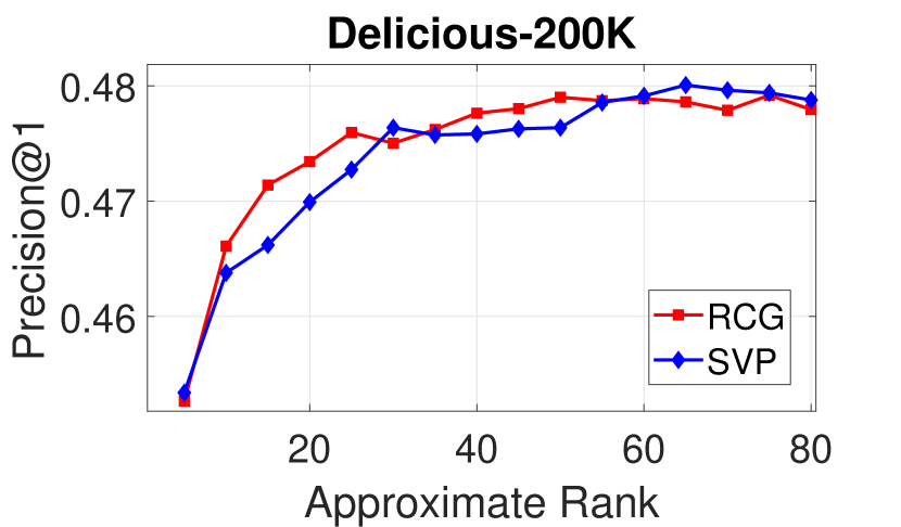
(a)

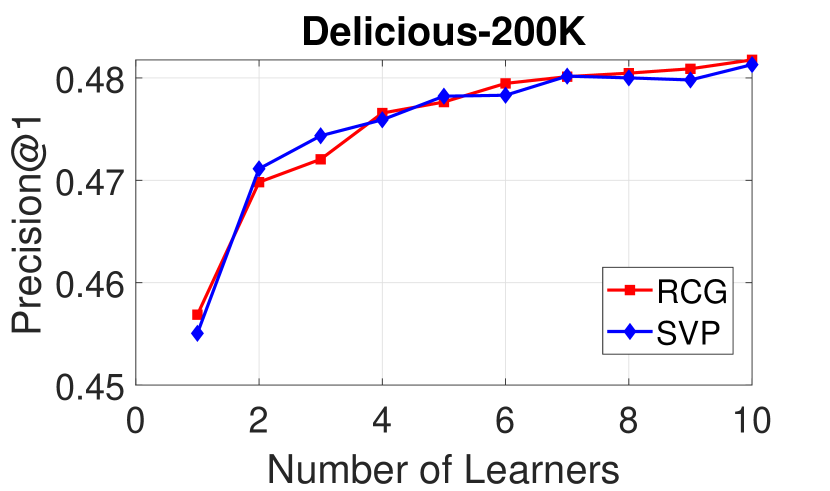
(b)

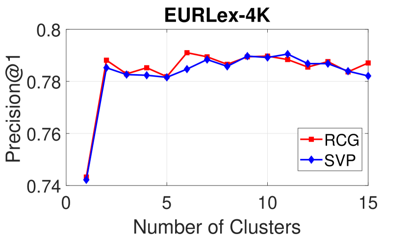
(c)

Figure 2: Variation of P@1 accuracy with embedding dimension, number of learners and number of clusters

Type	Embedding based					Tree Based			1-vs-All
ID	RXML	SLEEC	AnxML	ExML4	DXML	CFML	FXML	PFXML	Bonsai	DSMC	PPDS	PDS
1
P@1	65.84	65.77	-	-	66.03	62.94	64.41	63.14	-	-	-	61.29
P@3	40.08	40.29	-	-	40.21	38.21	39.38	40.11	-	-	-	35.82
P@5	29.26	29.38	-	-	27.51	27.72	28.79	29.38	-	-	-	25.74
2
P@1	67.16	66.91	64.94	66.17	68.17	67.88	68.51	60.31	-	-	-	51.82
P@3	61.02	61.12	59.63	59.87	62.02	62.00	63.44	56.08	-	-	-	44.18
P@5	56.38	56.40	55.01	54.85	57.45	57.32	59.06	53.41	-	-	-	38.95
3
P@1	86.90	87.00	86.82	85.22	88.73	86.51	84.12	83.77	-	81.86	86.50	81.86
P@3	72.50	72.69	69.72	68.31	74.05	71.61	67.46	67.57	-	62.52	68.40	62.52
P@5	58.22	58.58	55.74	54.21	58.83	57.62	53.42	53.51	-	45.11	53.20	45.11
4
P@1	79.10	79.36	80.04	78.41	-	78.73	70.94	70.07	83.01	82.40	83.83	73.38
P@3	64.37	64.68	64.26	61.49	-	64.96	59.90	59.13	69.38	68.50	70.72	60.28
P@5	52.27	52.94	52.71	50.30	-	53.65	50.31	50.37	58.31	57.70	59.21	50.35
5
P@1	86.31	86.43	86.48	86.66	86.45	84.82	82.97	71.78	84.66	85.20	-	77.75
P@3	74.20	73.91	74.26	75.07	70.88	73.57	67.71	59.30	73.70	74.60	-	65.46
P@5	63.64	63.37	64.19	64.62	61.31	63.73	57.66	51.04	64.54	65.90	-	55.28
6
P@1	47.86	47.61	46.64	47.73	48.13	47.87	43.09	17.94	46.69	45.50*	-	-
P@3	42.10	42.07	40.79	41.27	43.85	41.28	38.60	17.40	39.88	38.70*	-	-
P@5	39.30	39.35	37.65	37.93	39.83	38.01	36.18	16.99	36.38	35.50*	-	-
7
P@1	34.79	34.63	42.08	38.92	37.67	37.98	36.60	36.25	45.58	44.70*	45.32	-
P@3	31.18	30.90	36.62	34.30	33.72	34.05	32.84	33.56	40.39	39.70*	40.37	-
P@5	28.60	28.26	32.77	30.98	29.86	31.35	29.93	31.42	36.60	36.10*	36.92	-
8
P@1	89.87	89.94	93.54	92.45	-	92.78*	93.09	85.60	92.98	93.40*	92.72	89.29
P@3	75.69	75.82	78.37	77.43	-	78.48*	78.18	75.23	79.13	79.10*	78.14	74.09
P@5	61.28	61.48	63.31	62.63	-	63.58*	63.42	62.87	64.46	64.10*	63.41	60.12

Table 2: Precision Scores of various methods. Here AnxML stands for AnnexML, ExML4 stands for ExMLDS-4, CFML stands for CRAFTML, FXML stands for FastXML, PFXML stands for PfastreXML, DSMC stands for DiSMEC, PPDS stands for PPDSparse, PDS stands for PDsparse. The missing entries indicate that the results were not reported in the source. * indicates that the particular method did not run successfully on our machine, so the reported score is taken from the source.

5.3 Results

It is to be noted that for the methods indicated in Table 3, the scores obtained during their execution are reported in Table 2. In other cases the scores are copied for either from [8] or the source paper.

5.3.1 Comparison with Embedding-based methods

The results for SLEEC in Table 3 show orders of magnitude speed-up in train and test times compared to that reported in [17]. This is done by simply parallelizing the training and prediction phase over learners. RXML is 1.5 to 2 times faster than SLEEC in train time on large datasets with similar precision scores. In comparison with AnnexML and ExMLDS-4, RXML train times are faster by 1.5 to 4 times on large dataset, and RXML model size smaller by 3 to 10 times except for EURLex-4K. The comparison with DXML is ambiguous as the code is not published and it runs on GPU. Even then the train times of DXML are reported to be much higher on Wiki10-31K, Delicious-200K and Amazaon-670K with similar scores on all datasets except for Amazon-670K.

5.3.2 Comparison with Tree-based methods

Again in comparison to the results reported in [17], FastXML and PfastreXML run orders of magnitude faster with similar scores on 20 cores. RXML is very competitive with the state-of-the-art Tree-based methods. On EURLex-4K and Wiki10-31K both FastXML and PfastreXML are faster in terms of train times, but RXML scores achieves a better score. CRAFTML is slower in train time on Delicious-200K and the prediction times are generally 10 to 15 times slower than RXML. The memory constraints prevents us from running CRAFTML on AmazonCat-13K.

5.3.3 Comparison with 1-vs-All methods

PDSparse is slow compared to RXML in train time, but it is slightly faster in prediction. Bonsai is slower in both train and test times compared to RXML. Memory constraints prevented us from running PDSparse on Delicious-200K and Amazon-670K, and Bonsai on Delicious-200K, Amazon-670K, and AmazonCat-13K.

5.3.4 Comparison with Deep Learning methods

The state-of-the-art deep learning methods such as AttentionXML, LightXML and X-Transformer achieve the highest precision scores, but the train times are also significantly higher compared to RXML. In [30], it is shown that AttentionXML takes 26 hours to train on Amazon-670K, whereas LightXML takes 28 hours.

Type	Embedding based					Other
Language	MATLAB & C		C++		Python	Java	C/C++
Data ID	RXML	SLEEC	AnxML	EXML4	DXML*	CFML	FXML	PFXML	Bonsai	PDS
4
Train (s)	65.8	715	146	106	-	28	18.3	19	73.9	313
Test (ms)	0.48	0.86	0.05	0.05	-	6.56	0.47	0.13	0.99	0.21
Size (MB)	120	120	85.8	85.8	-	30	218	255	23.5	25
5
Train (s)	132	194	798	748	3047	47	59.3	65.8	2784	3558
Test (ms)	0.68	0.66	0.13	0.16	2.46	15.1	0.69	2.06	24.4	0.47
Size (MB)	262	262	611	611	-	-	482	1071	108	-
6
Train (s)	1091	1607	4382	4335	14537	2753	977	1054
Test (ms)	0.68	0.79	0.15	0.16	14.6	11.1	0.68	1.91	MLE	MLE
Size (GB)	1.84	1.84	10.7	10.7	-	0.34	6.2	14.5
7
Train (s)	1095	2250	1629	1609	67038	848	803	851
Test (ms)	0.71	0.75	0.07	0.09	23.3	7.64	1.12	1.65	MLE	MLE
Size (GB)	6.05	6.05	6.70	6.70	-	0.49	9.31	10.7
8
Train (s)	3097	6937	4289	4286	-		1696	1719		5631
Test (ms)	0.62	0.64	0.07	0.08	-	MLE	0.44	0.50	MLE	0.42
Size (GB)	5.91	5.91	18.4	18.4	-		18.3	18.9		0.001

Table 3: Train Time, Test Time(per sample), and Model Size. MLE stands for Memory Limit Exceeded. MLE happens when the memory requirements exceeds 120GB RAM.

6 Conclusion

We presented a novel Riemannian approach to Extreme classification problem, and applied it to several large scale, real world datasets. The method makes use of the underlying geometry of the SLEEC [33] model to perform the optimization faster, and uses a generalization of the conjugate gradient algorithm to matrix manifolds. The model performed comparably to other well known methods, while being significantly faster to train. The method also scales well with increasing number of labels. A similar structure may also exist in other Extreme Classification models, and can be exploited to develop other variants.

References

- [1] Boumal, N.: An introduction to optimization on smooth manifolds, (2020). Accessed online from http://www.nicolasboumal.net/book
- [2] Vandereycken, B.: Low-rank matrix completion by Riemannian optimization. In: SIAM Journal on Optimization, vol. 23, pp. 1214–1236 (2013). \doi10.1137/110845768
- [3] Boumal, N. and Mishra, B. and Absil, P.-A. and Sepulchre, R.: Manopt, a Matlab Toolbox for Optimization on Manifolds. In: Journal of Machine Learning Research, vol. 15, pp. 1455–1459 (2014). https://www.manopt.org
- [4] Boumal, N. and Absil, P.-A.: Low-rank matrix completion via preconditioned optimization on the Grassmann manifold. In: Linear Algebra and its Applications, vol. 475, pp. 200–239 (2015). \doi10.1016/j.laa.2015.02.027
- [5] Absil, P.-A., Mahony, R. and Sepulchre, R.: Optimization Algorithms on Matrix Manifolds. Princeton University Press, Princeton, NJ (2008). Accessed online from https://press.princeton.edu/absil
- [6] Massart, Estelle and Absil, P.-A.: Quotient Geometry with Simple Geodesics for the Manifold of Fixed-Rank Positive-Semidefinite Matrices. In: SIAM Journal on Matrix Analysis and Applications, vol. 41, pp. 171–198 (2020). \doi10.1137/18M1231389
- [7] Journée, M., Bach, F., Sepulchre, R.and Absil, P.-A.: Low-Rank Optimization on the Cone of Positive Semidefinite Matrices. In: SIAM Journal on Optimization, vol. 20, pp. 2327–2351 (2010).
- [8] Bhatia, K. and Dahiya, K. and Jain, H. and Mittal, A. and Prabhu, Y. and Varma, M.: The extreme classification repository: Multi-label datasets and code. (2016). http://manikvarma.org/downloads/XC/XMLRepository.html
- [9] Chen, Y., Lin, H.: Feature-aware Label Space Dimension Reduction for Multi-label Classification. In: Advances in Neural Information Processing Systems, pp. 1529–1537, (2012).
- [10] Tai, F., Lin, H.: Multilabel Classification with Principal Label Space Transformation. In: Neural Computation, vol. 24, issue 9, pp. 2508-2542, (2012).
- [11] Bi, W., Kwok, J.-T.: Efficient Multi-Label Classification with Many Labels. In: Proceedings of the 30th International Conference on International Conference on Machine Learning, pp. 405-413, (2013).
- [12] Balasubramanian, K., Lebanon, G.: The Landmark Selection Method for Multiple Output Prediction. In: Proceedings of the 29th International Coference on International Conference on Machine Learning, pp. 283-290, (2012).
- [13] Hsiang-Fu Yu, Prateek Jain, Inderjit S. Dhillon, Large-scale Multi-label Learning with Missing Labels. In: arXiv, 1307.5101, (2013).
- [14] Mineiro, P., Karampatziakis, N.: Fast Label Embeddings for Extremely Large Output Spaces, In: arXiv, 1412.6547, (2014).
- [15] Y. Prabhu, A. Kag, S. Harsola, R. Agrawal and M. Varma. Parabel: Partitioned label trees for extreme classification with application to dynamic search advertising. In Proceedings of the International World Wide Web Conference, Lyon, France, April 2018
- [16] Babbar, R., Schölkopf, B.: DiSMEC: Distributed Sparse Machines for Extreme Multi-label Classification, In: WSDM, (2016).
- [17] Yen, Ian E.H. and Huang, Xiangru and Dai, Wei and Ravikumar, Pradeep and Dhillon, Inderjit and Xing, Eric, PPDsparse: A Parallel Primal-Dual Sparse Method for Extreme Classification, In: Proceedings of the 23rd ACM SIGKDD International Conference on Knowledge Discovery and Data Mining, pp. 545–553, (2017).
- [18] Khandagale, S., H. Xiao and R. Babbar. “Bonsai: diverse and shallow trees for extreme multi-label classification.” Machine Learning (2020):
- [19] Y. Prabhu, A. Kag, S. Gopinath, K. Dahiya, S. Harsola, R. Agrawal and M. Varma. Extreme Multi-label Learning with Label Features for Warm-start Tagging, Ranking & Recommendation. In Proceedings of the ACM International Conference on Web Search and Data Mining, Los Angeles, United States, February 2018.
- [20] H. Jain, Y. Prabhu, and M. Varma, Extreme Multi-label Loss Functions for Recommendation, Tagging, Ranking & Other Missing Label Applications. In Proceedings of the ACM SIGKDD International Conference on Knowledge Discovery and Data Mining, pp 935-944, (2016).
- [21] Siblini, W., Meyer, F., Kuntz, P.: CRAFTML, an Efficient Clustering-based Random Forest for Extreme Multi-label Learning, In: ICML, (2018).
- [22] Y. Prabhu, and M. Varma, FastXML: A Fast, Accurate and Stable Tree-classifier for eXtreme Multi-label Learning, In Proceedings of the ACM SIGKDD International Conference on Knowledge Discovery and Data Mining, (2014).
- [23] Tagami, Y.: AnnexML: Approximate Nearest Neighbor Search for Extreme Multi-label Classification, In: Proceedings of the ACM SIGKDD International Conference on Knowledge Discovery and Data Mining, pp 455-464, (2017).
- [24] You, R., Zihan Zhang, Ziye Wang, Suyang Dai, H. Mamitsuka and Shanfeng Zhu. “AttentionXML: Label Tree-based Attention-Aware Deep Model for High-Performance Extreme Multi-Label Text Classification.” NeurIPS (2019).
- [25] Gupta, V., Wadbude, R., Natarajan, N., Karnick, H., Jain, P., & Rai, P. Distributional Semantics Meets Multi-Label Learning. In Proceedings of the AAAI Conference on Artificial Intelligence, 33(01), 3747-3754, (2019)
- [26] Wenjie Zhang, Junchi Yan, Xiangfeng Wang, and Hongyuan Zha. 2018. Deep Extreme Multi-label Learning. In Proceedings of the 2018 ACM on International Conference on Multimedia Retrieval (ICMR ’18). Association for Computing Machinery 100–107.
- [27] Liu, J., Wei-Cheng Chang, Yuexin Wu and Yiming Yang. “Deep Learning for Extreme Multi-label Text Classification.” Proceedings of the 40th International ACM SIGIR Conference on Research and Development in Information Retrieval (2017)
- [28] Anshul Mittal, Kunal Dahiya, Sheshansh Agrawal, Deepak Saini, Sumeet Agarwal, Purushottam Kar, and Manik Varma. DECAF: Deep Extreme Classification with Label Features. In Proceedings of the 14th ACM International Conference on Web Search and Data Mining (WSDM ’21). (2021)
- [29] Wei-Cheng Chang, Hsiang-Fu Yu, Kai Zhong, Yiming Yang, and Inderjit S. Dhillon. 2020. Taming Pretrained Transformers for Extreme Multi-label Text Classification. In Proceedings of the ACM SIGKDD International Conference on Knowledge Discovery & Data Mining (KDD ’20).163–3171.
- [30] Jiang, Ting, De-qing Wang, Leilei Sun, Huayi Yang, Zhengyang Zhao and Fuzhen Zhuang. “LightXML: Transformer with Dynamic Negative Sampling for High-Performance Extreme Multi-label Text Classification.” (2021)
- [31] Hsu, D.-J. , KakadeS.-M., Langford, J., Zhang, T.: Multi-Label Prediction via Compressed Sensing, In: arXiv, 0902.1284, (2009).
- [32] Medini, T.K.R, Huang, Q., Wang, Y., Mohan, V., Shrivastava, A.: Extreme Classification in Log Memory using Count-Min Sketch: A Case Study of Amazon Search with 50M Products, In: Advances in Neural Information Processing Systems, pp. 13265-13275, (2019).
- [33] Bhatia, K., Jain, H., Kar, P., Varma, M. and Jain, P.: Sparse Local Embeddings for Extreme Multi-label Classification, In: Advances in Neural Information Processing Systems, pp. 730-738, (2015).
- [34] Jain, P., Meka, R., Dhillon, I.-S.: Guaranteed Rank Minimization via Singular Value Projection, In: International Conference on Neural Information Processing Systems, pp. 937-945, (2010).
- [35] Sprechmann, P., Litman, R., Yakar, T.B., Bronstein, A., Sapiro, G.: Efficient Supervised Sparse Analysis and Synthesis Operators, In: Proceedings of the 26th International Conference on Neural Information Processing Systems, pp. 908-916, (2013).
- [36] Xu, Chang and Tao, Dacheng and Xu, Chao, Robust Extreme Multi-Label Learning, In: Proceedings of the 22nd ACM SIGKDD International Conference on Knowledge Discovery and Data Mining, pp. 1275–1284, (2016).