The LOFAR LBA Sky Survey: Deep Fields I. The Boötes Field

We present the first sub-mJy ($\approx 0.7$ mJy beam^-1) survey to be completed below $100$ MHz, which is over an order of magnitude deeper than previously achieved for widefield imaging of any field at these low frequencies. The high-resolution ($15\times 15$ arcsec) image of the Boötes field at $34$–$75$ MHz is made from $56$ hours of observation with the LOw Frequency ARray (LOFAR) Low Band Antenna (LBA) system. The observations and data reduction, including direction-dependent calibration, are described here. We present a radio source catalogue containing $1,948$ sources detected over an area of $23.6$ deg², with a peak flux density threshold of $5\sigma$. Using existing datasets, we characterise the astrometric and flux density uncertainties, finding a positional uncertainty of $\sim 1.2$  arcsec and a flux density scale uncertainty of about $5$ per cent. Using the available deep $144$-MHz data, we identified $144$-MHz counterparts to all the $54$-MHz sources, and produced a matched catalogue within the deep optical coverage area containing $829$ sources. We calculate the Euclidean-normalised differential source counts and investigate the low-frequency radio source spectral indices between $54$ and $144$ MHz. Both show a general flattening in the radio spectral indices for lower flux density sources, from $\sim-0.75$ at 144-MHz flux densities between $100$ and $1000$ mJy to $\sim-0.5$ at 144-MHz flux densities between $5$ and $10$ mJy. Such flattening is attributable to a growing population of star forming galaxies and compact core-dominated AGN.

1 Introduction

The LOw Frequency ARray (LOFAR; van Haarlem et al., 2013) has been operating successfully for a number of years now and has already produced a number of interesting results, including the first releases of the full sky survey (Shimwell et al., 2017, 2019), and of a series of Deep Fields (Tasse et al., 2021; Sabater et al., 2021) produced by the Surveys Key Science Project (KSP). However, most of the imaging work to date has focused on the upper end of LOFAR’s frequency coverage, using the High Band Antenna (HBA) system, operating at 120–240 MHz. The greater challenges in imaging at lower frequencies have meant that, until recently, less work has focused on imaging with the Low Band Antenna (LBA) system at $10$–$75$ MHz. The lower sensitivity of the LBA dipoles and the wide field of view (FoV; $\sim 20$ deg²) of the LBA stations both compound the problem of correcting for the propagation errors introduced by the varying ionosphere above the array (e.g. Mevius et al., 2016; de Gasperin et al., 2018b). The magnetised plasma of the ionosphere causes, to first order, propagation delays (hence phase errors) inversely proportional to frequency ($1/\nu$), which vary on temporal scales of tens of seconds and spatial scales of a few arcminutes. This therefore requires several tens of different corrections to be determined and applied within the FoV of a single observation. Higher order effects, including Faraday rotation ($\propto 1/\nu^{2}$), are also non-negligible at these frequencies.

Early LBA work was limited to very bright sources, such as M87 (de Gasperin et al., 2012) and 3C 295 (van Weeren et al., 2014), and wider field imaging such as that of the Boötes field ($\sim 5$ mJy beam^-1 noise; van Weeren et al., 2014) did not have full ionospheric calibration. In contrast, HBA observations are now routinely processed to produce thermal-noise images with a pipeline (ddf-pipeline; Shimwell et al., 2019; Tasse et al., 2021) that was built using killMS (Tasse, 2014a, b; Smirnov & Tasse, 2015) for direction-dependent calibration and DDFacet (Tasse et al., 2018) for wide-field correction and imaging. Only recently have we successfully implemented these and other direction-dependent calibration and imaging algorithms to work at the lower frequencies of the LBA, leveraging advances in other software, including dppp (van Diepen et al., 2018) and WSClean (Offringa et al., 2014). Together with a full understanding of the systematic effects in LOFAR data (de Gasperin et al., 2018b, 2019), the application of direction-dependent calibration has led to a number of high-resolution ($\sim 15$  arcsec), low-noise ($\sim 1$ mJy beam^-1) images of several individual targets, including the Toothbrush cluster (de Gasperin et al., 2020a), Abell 1758 (Botteon et al., 2020) and the planetary system HD 80606 (de Gasperin et al., 2020b). This has also allowed for the start of the first LOFAR low-frequency wide-area surveys with the LOFAR LBA Survey (LoLSS; de Gasperin et al., 2021). Here we apply a modified version of the ddf-pipeline to significantly longer LBA observations than those published so far. This provides a crucial test of the expectation that the noise continues to decrease with integration time, and is not fundamentally limited by systematic effects.

Similar to the tiered approach being undertaken for surveys with the HBA, the LOFAR Two-metre Sky Survey (LoTSS; Shimwell et al., 2019), and its Deep Fields (Tasse et al., 2021; Sabater et al., 2021), we aim to complement LoLSS with several deep LBA observations of the LoTSS Deep fields (Boötes, ELAIS-N1 and Lockman Hole). This is the first such observation. This deep, very low-frequency radio imaging, in combination with the higher frequency LoTSS Deep fields, will enable low-frequency spectral indices to be determined for all sources detected at LBA and reveal rare, extreme-valued sources. This will provide unique data on the shape of the low-frequency spectra of star forming galaxies, AGN, and galaxy clusters that will help answer many questions related to these types of sources. LOFAR LBA surveys reach an order of magnitude deeper and achieve an order of magnitude higher resolution than previous surveys at these frequencies (VLSSr; Lane et al., 2014).

As one of several extragalactic deep fields spanning a few square degrees, there is a wealth of additional multi-wavelength data available for the Boötes field. This field was originally part of the National Optical Astronomy Observatory (NOAO) Deep Wide Field Survey (NDWFS; Jannuzi et al., 1999), which covered $\sim 9$ deg² in the optical and near-infrared $B_{W}$, $R$, $I,$ and $K$ bands. Further observations have since been obtained, including X-ray (Murray et al., 2005; Kenter et al., 2005), UV (GALEX; Martin et al., 2003), and mid-infrared (Eisenhardt et al., 2004; Martin et al., 2003) imaging. Moreover, the AGN and Galaxy Evolution Survey (AGES) has provided redshifts for 23,745 sources, including both normal galaxies and AGN, across 7.7 deg² of the field (Kochanek et al., 2012). As one of the LoTSS Deep Fields, high-quality photometric redshifts have been determined for over 2 million optical sources (Duncan et al., 2021). The Boötes field has been widely surveyed at radio wavelengths – with the WSRT at 1.4 GHz (de Vries et al., 2002) and the VLA at 1.4 GHz (Higdon et al., 2005) and 325 MHz (Croft et al., 2008; Coppejans et al., 2015). Additionally, Boötes is one of the LoTSS Deep Fields, with a sensitivity achieved thus far of 30 $\mu$Jy beam^-1 using the HBA at $144$ MHz (Tasse et al., 2021). Finally, the previous LOFAR LBA image of the Boötes field by van Weeren et al. (2014) at $54$–$70$ MHz covered $19.4$ deg² and reached a noise level of $4.8$ mJy beam^-1 with a beam size of $31\times 19$ arcsec.

The outline of this paper is as follows. In Section 2 we describe the LOFAR LBA observations covering the Boötes field. In Section 3 we describe the data reduction techniques employed to achieve the deepest possible image, with a focus on the development and execution of a robust and automated pipeline for the direction-dependent calibration and imaging. In Section 4 we present the final image and describe the source-detection method and the compilation of the source catalogue. This section also includes an analysis of the quality of the catalogue. The spectral index distribution and differential source counts are presented in Section 5. Finally, Section 6 summarises and concludes this work.

Throughout this paper, the spectral index, $\alpha$, is defined as $S_{\nu}\propto\nu^{\alpha}$, where $S$ is the source flux density and $\nu$ is the observing frequency.

2 Observations

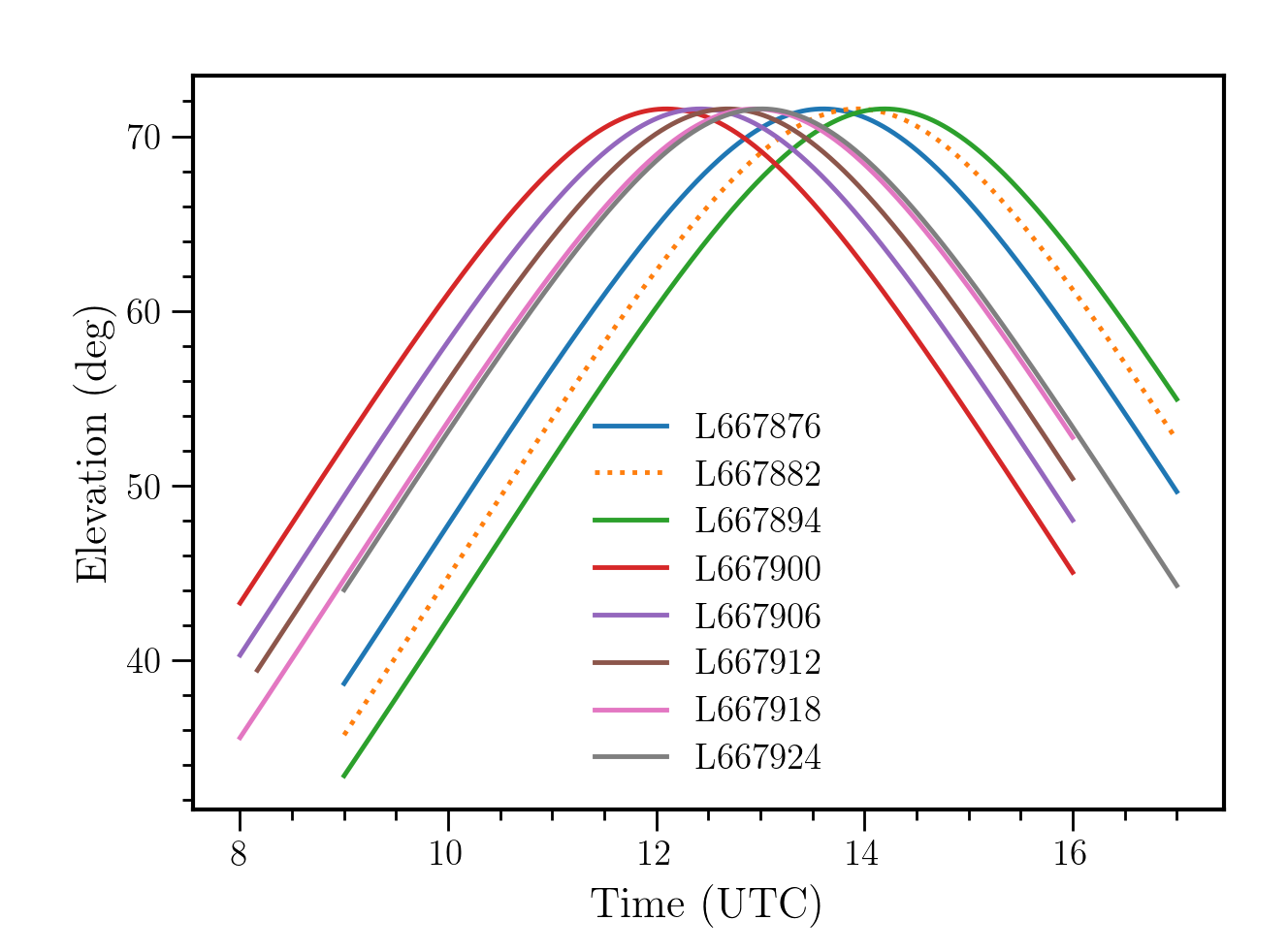
Figure 1: Elevation plots for the eight observations.

The Boötes field, at 14h32m03.0s +34d16m33s, was observed during September–October 2018 with the LOFAR Low Band Antenna (LBA) stations for a total of $64$ hr spread over eight observations of 8 hr each under Project code LC10_007. A summary of the observations is given in Table 1. Each eight-hour track was roughly centred at transit, with the elevation of the target field $\gtrsim 35$ deg (see Fig 1). All four correlation products (XX, XY, YX and YY) were recorded with the frequency band divided into $195.3125$ kHz-wide sub-bands (SBs) with each SB further divided into $64$ channels. The integration time used was $1$ s. These high time and frequency resolutions were selected to allow for the accurate removal of radio frequency interference (RFI). The maximum number of SBs for the system in $8$-bit mode is $488$ and the chosen strategy was to use $244$ for the Boötes field giving a total bandwidth of $48$ MHz between $30$ and $78$ MHz. The remaining $244$ SBs were used to observe the bright calibrator source, 3C 295, located $18.3$^∘ away, with a simultaneous station beam and an identical SB setup to the Boötes observation.

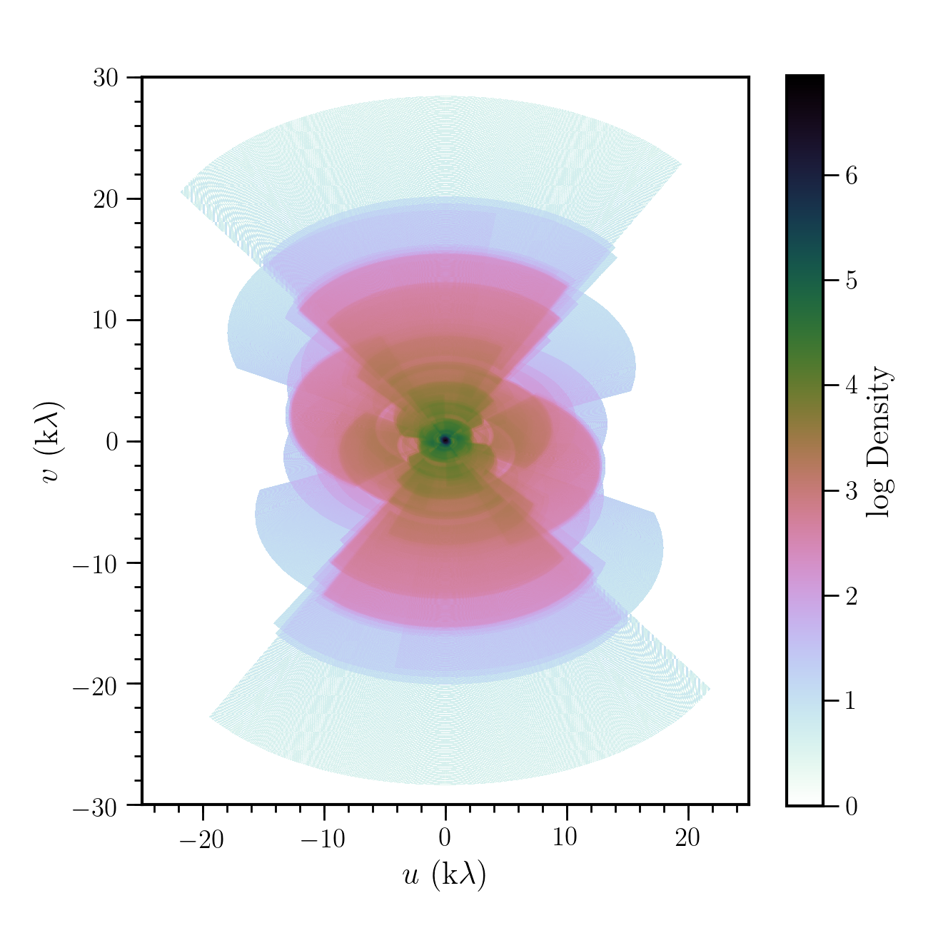
Figure 2: $uv$-coverage for one observation of the Boötes field. The maximum baseline is $120$ km (or $30$ k$\lambda$). The colour scale shows the logarithm of the density of points in $uv$-space.

The full Dutch array with $14$ remote and $24$ core stations was used for all observations, with between $34$ and $38$ total stations available for each observation (typical station failure rates). This setup results in baselines that range between $40$ m and $120$ km. The $uv$-coverage for one Boötes field observation is plotted in Fig. 2 – showing the usual dense inner coverage and outer extensions to the north and south due to the high density of core stations and the north–south extension of the Dutch remote stations. The maximum theoretical resolution achievable with such an array is $10$ arcsec at 60 MHz (varying between $20$ and $8$ arcsec between the lower and upper ends of the frequency band). Finally, the ‘LBA_OUTER’ configuration was employed, which uses the outer $48$ out of the $96$ LBA antennae in each station, giving a station diameter of $81$ m and a full width at half maximum (FWHM) of the field of view $\approx 4.3$^∘ at $54$ MHz (but varying from $\approx 7.8$ to $\approx 3.1$^∘ between $30$ and $75$ MHz).

Table 1: Observations of the Boötes field

ID	Start of Observation	Stations	Image noise
			(mJy beam-1)
L667876	28-Sep-2018/09:00	38	1.72
L667882	23-Sep-2018/09:00	34	2.48
L667894	19-Sep-2018/09:00	35	1.79
L667900	21-Oct-2018/08:00	37	1.82
L667906	16-Oct-2018/08:00	37	1.79
L667912	12-Oct-2018/08:10	35	1.72
L667918	08-Oct-2018/08:00	37	1.69
L667924	07-Oct-2018/09:00	37	1.67

3 Data reduction

3.1 Pre-processing

Initial pipeline pre-processing per SB for both the calibrator and target was carried out by the Netherlands Institute for Radio Astronomy (ASTRON) and included ‘demixing’ (a computationally fast method of removing bright ‘A-team’ sources by subtracting their contributions directly from the visibility data; van der Tol et al., 2007) of Cassiopeia A at a distance of $79^{\circ}$ and Cygnus A at $63^{\circ}$, flagging of RFI with aoflagger (Offringa, 2010; Offringa et al., 2012), and final averaging to $4$ s and $48.828$ kHz per channel. The final pre-processed data were stored in the LOFAR Long Term Archive (LTA; Belikov et al., 2011). Dysco (Offringa, 2016) compression was used resulting in a total data size per observation for both the target and calibrator of $\sim 300$ GB.

3.2 Direction-independent calibration

After download from the archive, the data were processed using prefactor version 3 (v3) to perform further flagging, calibration, and averaging. The prefactor pipeline is built within the LOFAR genericpipeline framework to describe the workflow, and relies heavily on casacore tables and measurement sets (MSs; van Diepen, 2015) and the Default Pre-Processing Pipeline (dppp; van Diepen et al., 2018) for individual operations. The full details of the method for calibrating direction-independent effects in LOFAR data —particularly LBA data— is described in detail by de Gasperin et al. (2019, 2020a) and implemented in prefactor v3. Here, we summarise the steps, noting particular steps where the reduction diverged from the default HBA calibration, which is documented in detail elsewhere (e.g. Shimwell et al., 2019).

3.2.1 Calibrator processing

For all SBs of the calibrator beam, the first step was to flag any data from known bad stations (CS013 and CS031 in all observations), data at low elevations ($<20$ deg) and data with extremely low amplitudes ($<10^{-30}$). aoflagger was then run on a virtually concatenated MS of all SBs to remove RFI across the full bandwidth using the LBAdefaultwideband strategy. No additional averaging was done so the calibrator data remain at a resolution of $4$ s and $48.82$ kHz per channel ($4$ channels per SB).

The model used for calibration of 3C 295 consisted of two point-source components separated by $3.93$ arcsec and was normalised to the flux scale of Scaife & Heald (2012, hereafter SH12). The visibilities of this model are predicted with dppp and stored in the MODEL_DATA column of the MS for efficiency.

The following steps of the calibrator pipeline were then to solve sequentially for the following effects:

1. polarisation alignment (PA) – a time-independent frequency-dependent ($\propto\nu$) term that corrects for the misalignment between the XX and YY polarisations due to different station calibration for the independent feeds,

2. Faraday rotation (FR) – a direction-, time-, and frequency-dependent ($\propto\nu^{-2}$) term that corrects for the phase rotation caused by the ionosphere,

3. bandpass (B) – a time-independent, frequency-dependent term that, for the LBA, largely corrects for the dipole response (strongly peaked at $\sim 60$ MHz, cf. fig. 20 of van Haarlem et al., 2013),

4. and phase (P) – a time- and frequency-dependent scalar term that incorporates both the effects of the ionosphere ($\propto\nu^{-1}$ to first order) and instrumental clock errors ($\propto\nu$).

At each point, the previously determined correction(s) were applied before solving for the next term. Gain solutions were derived with dppp ddecal to determine the diagonal and rotation terms for the polarisation alignment and Faraday rotation steps, and diagonal-only terms for the bandpass and ionosphere steps at the full frequency and time resolution. To improve the signal-to-noise ratio, at each calibration step initially the DATA (the pre-processed visibilities), and subsequently CORRECTED_DATA (the pre-processed visibilities with the previously determined correction(s) applied) were first smoothed with a Gaussian kernel both in time and frequency in a baseline-dependent way before solving, that is the shorter baselines were smoothed with larger kernels than the longer baselines. The corrections were derived from the raw gain solutions with losoto. The final P solutions are decomposed into the contributing ionosphere and clock terms, making use of their different frequency dependence ($\propto 1/\nu$ and $\propto\nu$ respectively). Although these terms are not applied separately to the target visibilities, they are effectively corrected for by applying the time- and frequency-dependent phase solutions. These terms also provide a useful diagnostic as to the severity of the ionospheric effects during each observation.

3.2.2 Target calibration

In the same way as for the calibrator data, for all SBs of the target beam, the first step of the pipeline was to flag any data from known bad stations (CS013 and CS031 in all observations), data at low elevations ($<20$ deg), and data with extremely low amplitudes ($<10^{-30}$). The calibration solutions from the corresponding simultaneous calibrator beam were then applied to each target observation, in the following order: PA, B, and P. We did not apply the FR because this is a direction-dependent effect. We note that, unlike the procedure for HBA processing, because the calibrator is observed simultaneously, we correct the target field with the phases from the calibrator. While these contain the instrumental clock delays that are independent of direction, they also contain the ionospheric delays in the direction of the calibrator. Any further ionospheric phase solutions calculated for the target field will therefore be differential with respect to the direction of 3C 295; however, the frequency-dependence will remain the same. The data were then corrected for the station beams. No additional averaging was done so the data remain at a resolution of $4$ s and $48.82$ kHz per channel ($4$ channels per SB).

HBA processing usually follows this stage with a step to predict the visibilities from bright A-team sources and flag periods with high contributions. However, as the LBA data had already been demixed in pre-processing, this was not necessary. The data were then concatenated into bands of $2$ MHz, and aoflagger was run on a virtually concatenated MS of all bands to remove any remaining RFI, again using the LBAdefaultwideband strategy across the full bandwidth.

We did not use prefactor for the final calibration of the target field, but rather used the Libraries for Low Frequency (LiLF) framework for its ease of testing different strategies. We used BLSmooth to do a baseline-based smoothing of the visibilities before solving for scalarphase only and used a model for the field from the Global Sky Model that included information from TGSS, WENSS, NVSS, and VLSS. We included sources predicted to be above $0.5$ Jy at $60$ MHz within a radius of $0.67$ times the FWHM of the station beam at $34$ MHz. Phases were solved for on a timescale of $12$ s and within frequency blocks of $0.5$ MHz. We note that this is the highest time resolution used in the data reduction so any errors still present at these timescales cannot be removed later in the direction-dependent calibration.

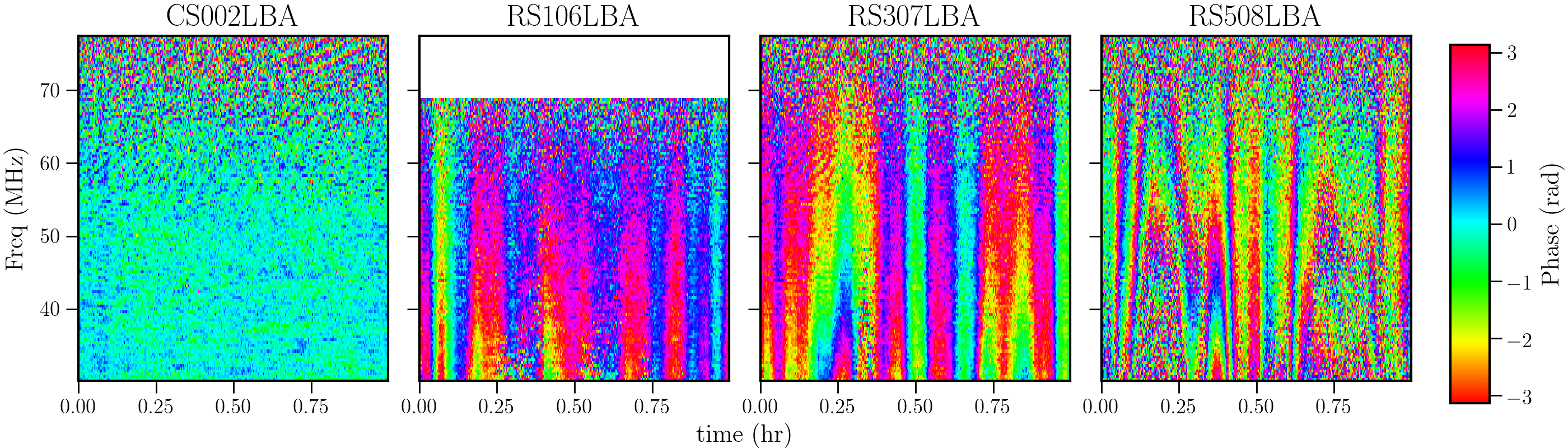
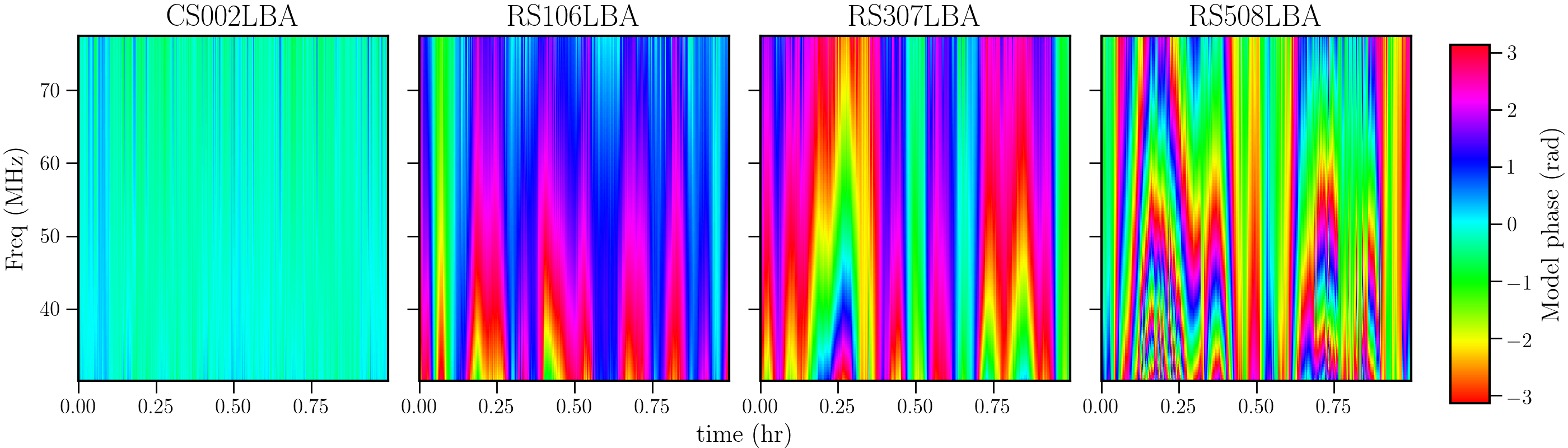
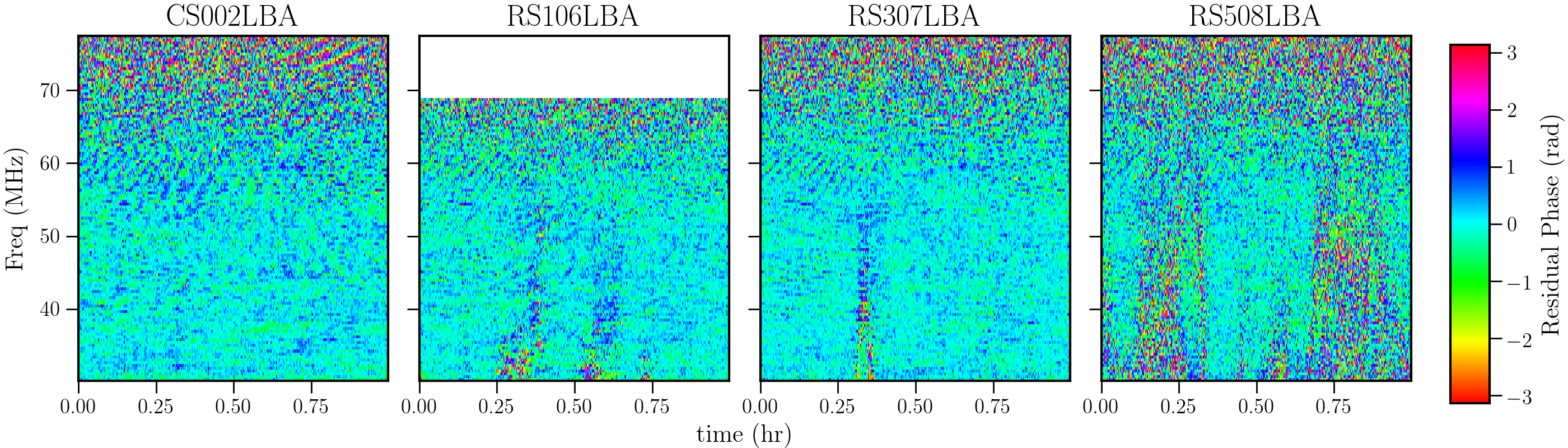
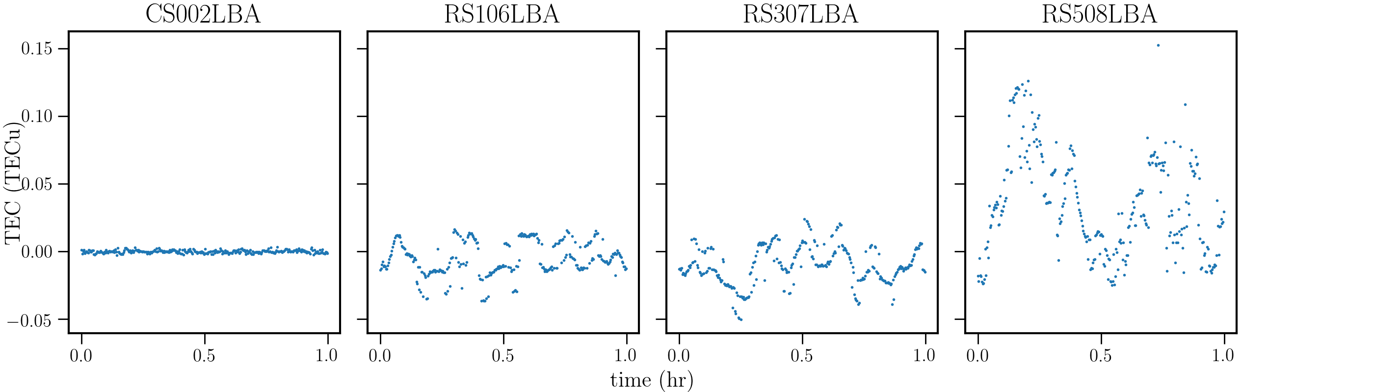
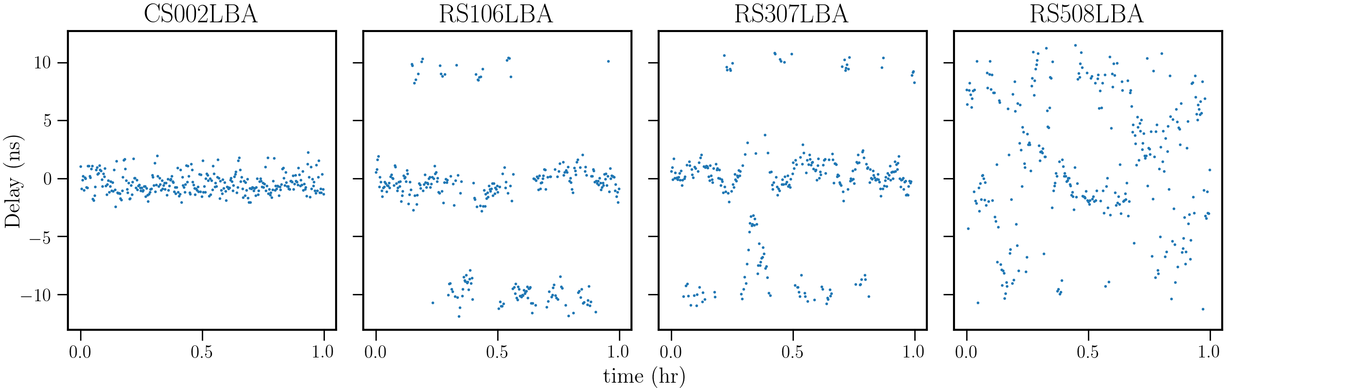
Figure 3: Example direction-independent phase solutions on the target field, taken from the fourth hour of observation L667924. From top to bottom the panels show the raw phase solutions, the TEC+Delay model phases, the phase residuals, and the fitted TEC and Delay terms as a function of time.

Experience has shown that a single total electron content (TEC) term is insufficient to characterise the phase solutions, and so we decompose the scalar phases into a TEC ($\propto 1/\nu$) term and a delay ($\propto\nu$) term. The origin of this delay term is not fully understood because the instrumental clock errors are corrected when the phases are transferred from the calibrator. It may be a geometric delay due to pointing errors. An example of the scalar phase solutions and fitted TEC and delay terms is shown in Fig. 3 for a single one-hour chunk of data from one observation that is representative of the general quality of the solutions. We note that, particularly for remote stations, the delay solutions during some time periods (most often at low elevation) can be very noisy, even random. This may be due to improperly modelled phases (Faraday rotation and higher order ionospheric effects are not modelled here), poor signal-to-noise ratio, or strongly direction-dependent effects that mean a single correction for the field is insufficient. While the noisy data result in discrete ‘jumps’ in the TEC and Delay solutions, due to the incorrect local minimum found in the fit, the overall residual phases are mostly flat and noise-like and are flatter than after a TEC-only fit. Once these solutions had been determined, the unsmoothed visibility data were then corrected for the combined TEC and delay.

3.3 Direction-dependent calibration

The data were further processed using a slightly modified version of version 2.2 of the standard Surveys KSP pipeline, ddf-pipeline as described by Shimwell et al. (2019) and Tasse et al. (2021). This pipeline carries out direction-dependent calibration using killMS (Tasse, 2014a, b; Smirnov & Tasse, 2015) and imaging is done using DDFacet (Tasse et al., 2018). Version 2.2 of the pipeline makes use of enhancements to the calibration and imaging —particularly of extended sources— that were described briefly in section 5 of Shimwell et al. (2019) and discussed more fully by Tasse et al. (2021). The implementation and modifications we made are described here in detail.

We first processed each of the eight observations separately. This provides information on the variation of quality between observations. We adopt a very conservative approach and use only five directions with the same facet layout for each of the eight observations. The small number of directions is a trade-off between the facet size, which is large (approximately $4$–$6$ square degrees), and $S/N$. To process a single observation, we configured the pipeline to perform two cycles of phase-only self-calibration, with imaging at a lower resolution ($30$ arcsec), followed by one cycle of phase-only calibration and imaging at $15$  arcsec. Solutions in both cases are obtained on timescales of $2$ min and within each $2$-MHz band. In practice, full-Jones solutions are calculated, but the amplitudes are set to unity and only the phases are applied in imaging. The phase component of the solutions is smoothed with a TEC-like function, that is $1/\nu$, over the full bandwidth. A final very slow full-Jones calibration is performed, providing both phase and amplitude solutions on timescales of $43$ min. Unlike the standard LoTSS-DR2 processing, we do no additional direction-independent calibration; we apply amplitude corrections only on the very long timescale, and we use the full bandwidth already in the initial steps. As the LBA beam model is better understood than that of the HBA, we did not apply the bootstrapping of the flux-density scale usually done for the HBA. We only processed bands 2–22 ($34$–$75$ MHz), avoiding the low-$S/N$ high-frequency bands (where the dipole response rapidly drops off; cf. fig. 20 of van Haarlem et al., 2013) and the low-frequency end where the ionospheric effects become too large (in particular Faraday rotation). The noise levels achieved in each eight-hour observation, listed in Table 1, mostly vary between 1.67 and 1.82 mJy beam^-1, with one strong outlier of 2.48 mJy beam^-1 for L667882. We therefore excluded this observation from further processing.

To process the seven remaining observations together, we configured the pipeline in the deep-imaging mode (as described in Tasse et al., 2021) using the image from the best single observation (L667924) as a starting model. Each $2$-MHz band is calibrated against this model: first for the $2$ min phase-only solutions, again smoothed with a TEC-like function, followed by the $43$ min amplitude and phase solutions. Final imaging is done at $15$ arcsec resolution. In the final imaging step, we applied a per-facet position offset using this capability in DDFacet. For LoTSS-DR1 and the LoTSS Deep Fields, the per-facet offsets are derived relative to Pan-STARRs (Chambers et al., 2016). However, the resolution of the LBA image is too low and the Pan-STARRS source density too high to achieve unique matches. Instead, the per-facet offsets were derived with respect to the positions of compact sources in the $6$  arcsec resolution deep HBA image of the Boötes field (Tasse et al., 2021) – compact sources were selected as those with size $<10$ arcsec. In summary, after generating a source catalogue using PyBDSF and selecting good sources (positional error $<3$  arcsec and size $<20$  arcsec), the LBA sources were matched to the HBA compact sources taking the nearest source within $10$  arcsec, and Gaussians fitted to the position offset distributions. This is implemented within ddf-pipeline. Around $50$ matches within each facet were found, and were of the order of $1$–$3$  arcsec. These offsets were applied on a per-facet basis in the final round of DDFacet imaging.

3.4 Final image and catalogue

The final beam-corrected image at $15\times 15$ arcsec resolution is shown in Fig. 4 and is masked where the primary beam correction exceeds $3$. This image is available online. A small portion of the image covering the inner $0.25$ deg² is shown in Fig. 5 to illustrate the resolution and quality of the image. The rms noise level in the central part is relatively smooth with a median value of $\sim 0.70$ mJy beam^-1 within the innermost square degree, and $50$% of the map is at a noise level below $1.2$ mJy beam^-1 (see also Fig. 6). There remain some strong phase artefacts and corresponding increases in noise level around the brightest sources; these were not entirely removed during the direction-dependent calibration, but are localised.

Figure 4: Colour-scale map showing the full primary-beam-corrected image. The image covers $23.6$ deg². The colour scale shows the intensity from $-3\sigma_{\mathrm{cen}}$ to $25\sigma_{\mathrm{cen}}$ where $\sigma_{\mathrm{cen}}=0.7$ mJy beam^-1 is the approximate rms in the image centre. The black polygons show the facets used in the calibration and imaging.

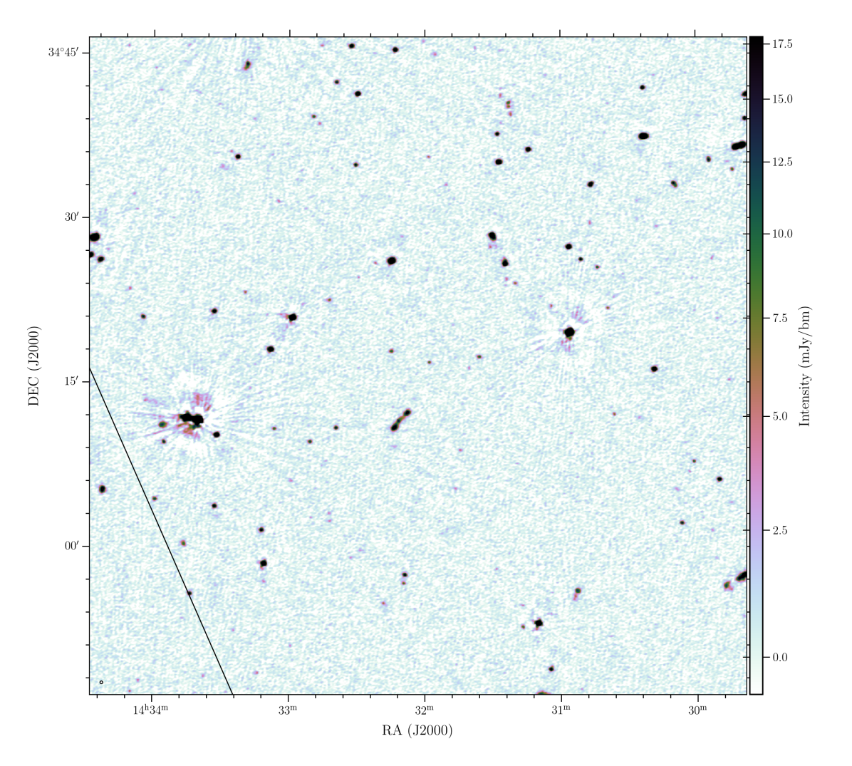
Figure 5: Zoom-in of the central part of the primary-beam-corrected image. The image covers $1$ deg². The colour scale shows the flux density from $-3\sigma_{\mathrm{cen}}$ to $25\sigma_{\mathrm{cen}}$ where $\sigma_{\mathrm{cen}}=0.7$ mJy beam^-1 is the approximate rms in the image centre. The black line shows one of the facet boundaries used in the calibration and imaging – even sources on or near the facet boundaries are well imaged.

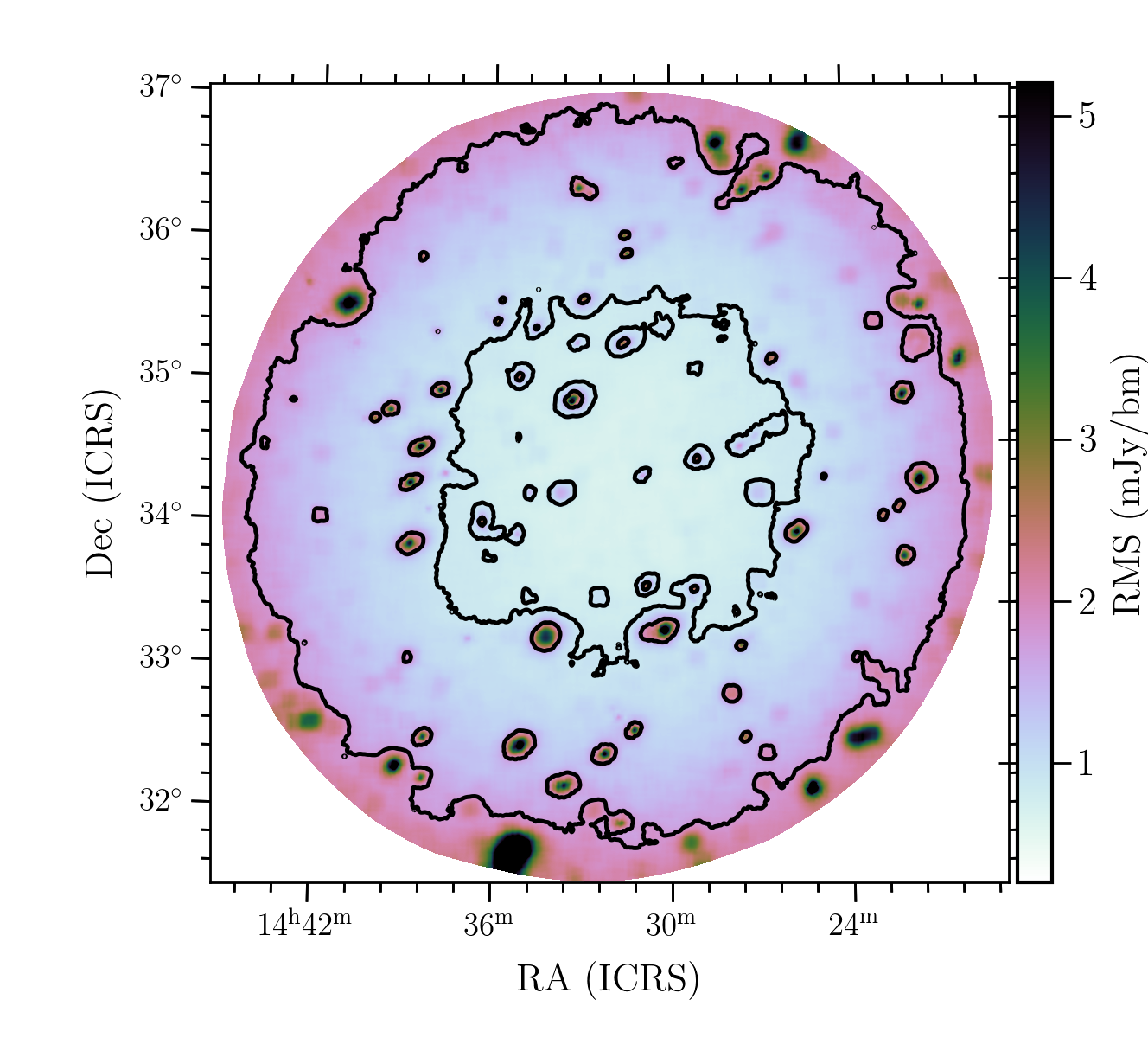
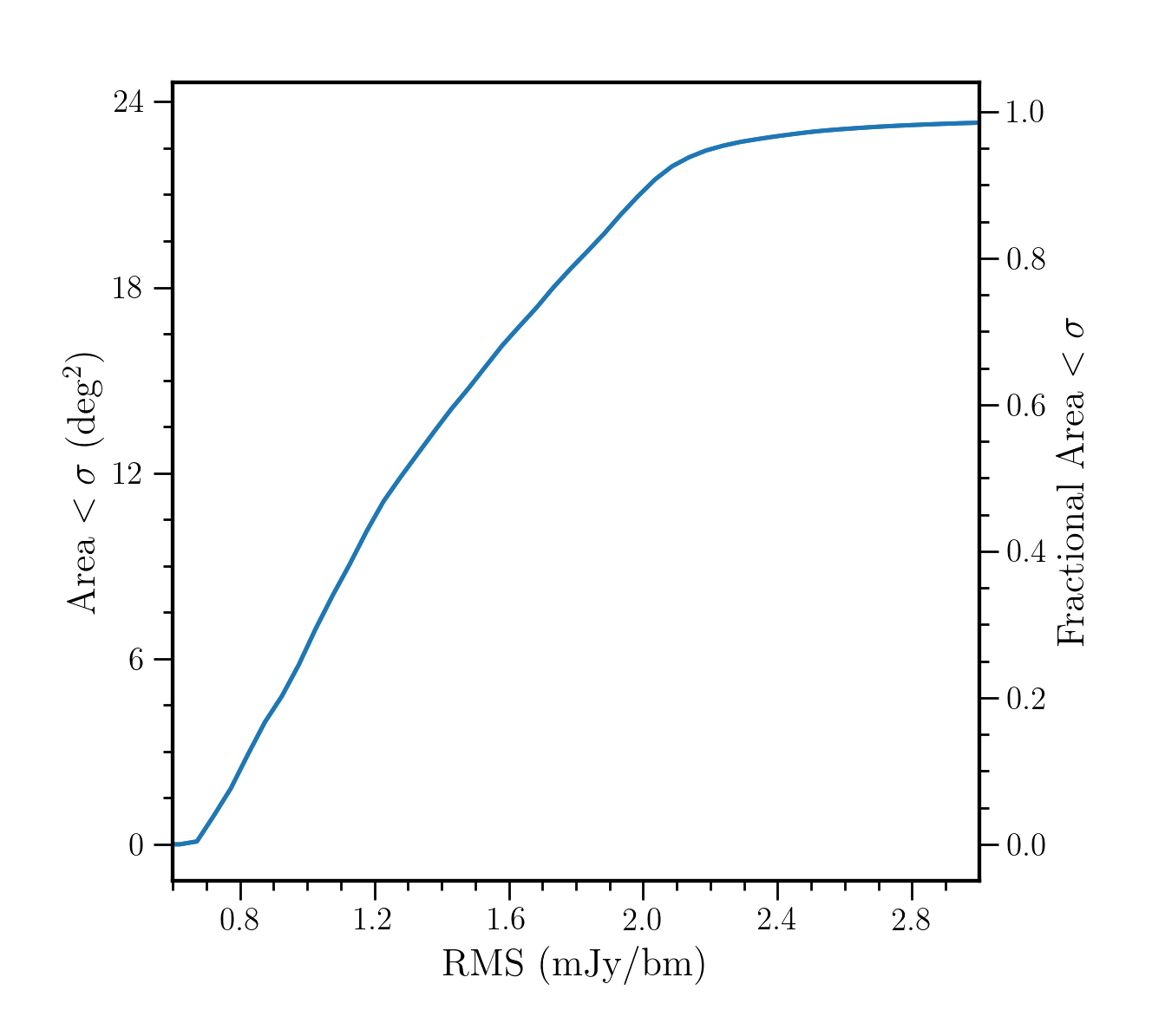
Figure 6: Left: Local rms noise measured in the final image. Contours are plotted at $0.9$ mJy beam^-1 and $1.8$ mJy beam^-1. Peaks in the local noise coincide with the locations of bright sources. Right: Cumulative area of the map with a measured rms noise level below the given value.

4 Source catalogue

To produce a catalogue of the radio sources we extracted sources from the final image using PyBDSF (Mohan & Rafferty, 2015). This was done using the standard HBA Surveys settings (Shimwell et al., 2019): that is with a peak detection threshold of $5\sigma$ and an island detection threshold of $4\sigma$. The background noise variations were estimated across the images using a sliding box with a box size of $30\times 30$ synthesised beams, which was decreased to $12\times 12$ synthesised beams in regions of high $S/N$ sources ($\geq 150$) in order to more accurately capture the increased noise level around bright sources. The PyBDSF wavelet decomposition was used to better characterise the complex low-surface-brightness extended emission. Source detection was done on the apparent sky image, while source parameters were extracted from the beam-corrected image. Figure 6 shows the variation in rms noise determined across the image. The increase in rms noise towards the edge of the field is a result of the ‘primary’ beam (LOFAR station beam). Errors on the fitted source shape parameters are computed following Condon (1997). The PyBDSF catalogue contains $1,948$ sources, with total flux densities between $3$ mJy and $18$ Jy. The PyBDSF source catalogue is available online¹¹. A sample of the catalogue, showing the brightest and faintest entries, is given in Table 2.

Table 2: Example entries from the full source catalogue.

Source Name	RA	$\sigma_{RA}$	DEC	$\sigma_{DEC}$	$S_{i}$		$S_{p}$		$\sigma_{\mathrm{local}}$	$N_{\mathrm{gauss}}$	$a$		$b$		$\phi$
	(deg)	( arcsec)	(deg)	( arcsec)	(mJy)		(mJy/bm)		(mJy/bm)		( arcsec)		( arcsec)		(deg)
(1)	(2)	(3)	(4)	(5)	(6)		(7)		(8)	(9)	(10)		(11)		(12)
LBABOO J143514.80+314052.3	$218.81167$	$0.2$	$31.68122$	$0.1$	$18395.2$ $\pm$	$231.8$	$4315.1$ $\pm$	$33.6$	$33.63$	$3$	$41.6$ $\pm$	$0.5$	$14.1$ $\pm$	$0.2$	$8.4$ $\pm$	$0.9$
LBABOO J144102.55+353046.0	$220.26061$	$0.0$	$35.51280$	$0.0$	$11964.8$ $\pm$	$56.2$	$8396.9$ $\pm$	$7.3$	$7.32$	$7$	$24.4$ $\pm$	$0.0$	$10.1$ $\pm$	$0.0$	$168.5$ $\pm$	$0.1$
LBABOO J143410.44+331144.9	$218.54351$	$0.1$	$33.19582$	$0.3$	$7139.8$ $\pm$	$137.2$	$1350.0$ $\pm$	$4.3$	$4.29$	$8$	$62.4$ $\pm$	$0.8$	$19.7$ $\pm$	$0.2$	$106.9$ $\pm$	$0.9$
LBABOO J143849.07+335015.5	$219.70445$	$0.0$	$33.83765$	$0.0$	$6743.7$ $\pm$	$33.5$	$4838.4$ $\pm$	$4.5$	$4.52$	$8$	$16.8$ $\pm$	$0.0$	$11.9$ $\pm$	$0.0$	$3.1$ $\pm$	$0.3$
LBABOO J143318.03+345102.5	$218.32514$	$0.4$	$34.85072$	$0.4$	$4744.6$ $\pm$	$45.5$	$997.9$ $\pm$	$4.9$	$4.94$	$6$	$94.9$ $\pm$	$1.3$	$13.6$ $\pm$	$0.2$	$133.8$ $\pm$	$0.8$
LBABOO J143334.56+320908.6	$218.39402$	$0.1$	$32.15239$	$0.2$	$3295.6$ $\pm$	$39.3$	$697.0$ $\pm$	$4.5$	$4.48$	$6$	$41.2$ $\pm$	$0.6$	$22.8$ $\pm$	$0.3$	$70.1$ $\pm$	$1.5$
LBABOO J142700.25+341202.0	$216.75104$	$0.1$	$34.20057$	$0.2$	$3114.7$ $\pm$	$15.5$	$410.8$ $\pm$	$1.3$	$1.30$	$9$	$78.9$ $\pm$	$0.5$	$22.8$ $\pm$	$0.1$	$46.8$ $\pm$	$0.4$
LBABOO J142519.37+320707.0	$216.33072$	$0.1$	$32.11863$	$0.2$	$2978.8$ $\pm$	$120.7$	$768.1$ $\pm$	$10.9$	$10.95$	$2$	$27.6$ $\pm$	$0.5$	$14.9$ $\pm$	$0.3$	$69.9$ $\pm$	$1.9$
LBABOO J143849.43+341553.3	$219.70596$	$0.0$	$34.26481$	$0.0$	$2930.8$ $\pm$	$34.3$	$1533.8$ $\pm$	$4.9$	$4.89$	$6$	$18.6$ $\pm$	$0.1$	$13.5$ $\pm$	$0.1$	$143.1$ $\pm$	$0.9$
⋮
LBABOO J142926.62+334405.8	$217.36094$	$2.4$	$33.73496$	$1.1$	$3.0$ $\pm$	$1.3$	$2.9$ $\pm$	$0.7$	$0.75$	$1$
LBABOO J143250.18+340241.5	$218.20909$	$1.8$	$34.04486$	$1.2$	$3.2$ $\pm$	$1.3$	$3.0$ $\pm$	$0.7$	$0.68$	$1$
LBABOO J142755.08+334853.9	$216.97950$	$2.1$	$33.81498$	$1.4$	$3.4$ $\pm$	$1.5$	$3.1$ $\pm$	$0.8$	$0.77$	$1$
LBABOO J143050.88+334700.8	$217.71200$	$2.1$	$33.78358$	$1.6$	$3.4$ $\pm$	$1.5$	$3.0$ $\pm$	$0.8$	$0.76$	$1$
LBABOO J143128.32+335759.4	$217.86799$	$1.2$	$33.96652$	$0.6$	$3.9$ $\pm$	$1.0$	$4.5$ $\pm$	$0.6$	$0.66$	$1$
LBABOO J143229.21+342436.3	$218.12169$	$0.9$	$34.41009$	$0.9$	$3.9$ $\pm$	$1.1$	$4.5$ $\pm$	$0.7$	$0.70$	$1$
LBABOO J142950.63+342049.6	$217.46098$	$2.7$	$34.34712$	$1.3$	$4.1$ $\pm$	$1.6$	$2.9$ $\pm$	$0.7$	$0.71$	$1$
LBABOO J142717.32+350125.2	$216.82216$	$1.9$	$35.02368$	$1.5$	$4.1$ $\pm$	$1.6$	$3.7$ $\pm$	$0.9$	$0.86$	$1$	$10.3$ $\pm$	$5.0$	$0.0$ $\pm$	$2.9$	$120.9$ $\pm$	$39.2$
LBABOO J143541.31+334228.0	$218.92214$	$1.6$	$33.70780$	$2.0$	$4.1$ $\pm$	$1.7$	$3.3$ $\pm$	$0.9$	$0.83$	$1$	$9.6$ $\pm$	$4.9$	$3.6$ $\pm$	$3.7$	$18.2$ $\pm$	$78.4$
LBABOO J143441.07+350146.7	$218.67111$	$2.0$	$35.02964$	$1.5$	$4.1$ $\pm$	$1.7$	$3.6$ $\pm$	$0.9$	$0.89$	$1$

4.1 Astrometric precision

We evaluated any source position errors or offsets induced by phase calibration errors by comparing the positions of sources in the LBA image with those in the $6$ arcsec-resolution deep HBA image of the Boötes field (Tasse et al., 2021). This image has an astrometric accuracy of $0.2$  arcsec with positions corrected in the imaging process relative to the optical Pan-STARRS catalogue (Chambers et al., 2016). We selected a sample of compact single-Gaussian sources with peak flux densities at least $7.5\sigma$ and smaller than $25$  arcsec.

From this sample of $480$ sources, we measured small offsets between the positions of the sources in the LBA and the HBA of $dRA=\alpha_{\mathrm{LBA}}-\alpha_{\mathrm{HBA}}=0.22\pm 0.05$ arcsec ($\sigma=1.17$ arcsec) and $dDEC=\delta_{\mathrm{LBA}}-\delta_{\mathrm{HBA}}=-0.02\pm 0.05$ arcsec ($\sigma=1.20$ arcsec) which is of the order of the pixel size of the LOFAR observations and the HBA accuracy ($\sim 0.2$ arcsec). The offsets are plotted in Fig. 7 and in Fig. 8 as a function of position on the sky. While a per-facet positional correction was made in the imaging (see Sect. 3.3), a trend in the declination offsets is still apparent within each facet, in that at higher declination the LBA positions are shifted slightly south ($\sim 1$  arcsec), while at lower declination, the LBA positions are shifted slightly north ($\sim 1$  arcsec). This is likely due to refraction and systematic ionospheric effects. Refraction causes lines of sight at greater zenith angles through the thicker projected ionosphere to be subject to greater deflection angles. As the observations are centred on transit, the right ascension offset should average out leaving only a bulk declination offset. Deflection angle differences of a few arcseconds over a degree are possible assuming a typical ionosphere height and thickness. Furthermore, the ionosphere typically has a strong north–south gradient in electron density during the daytime that may compound this effect. Smaller facet sizes would allow these effects to be corrected during self-calibration.

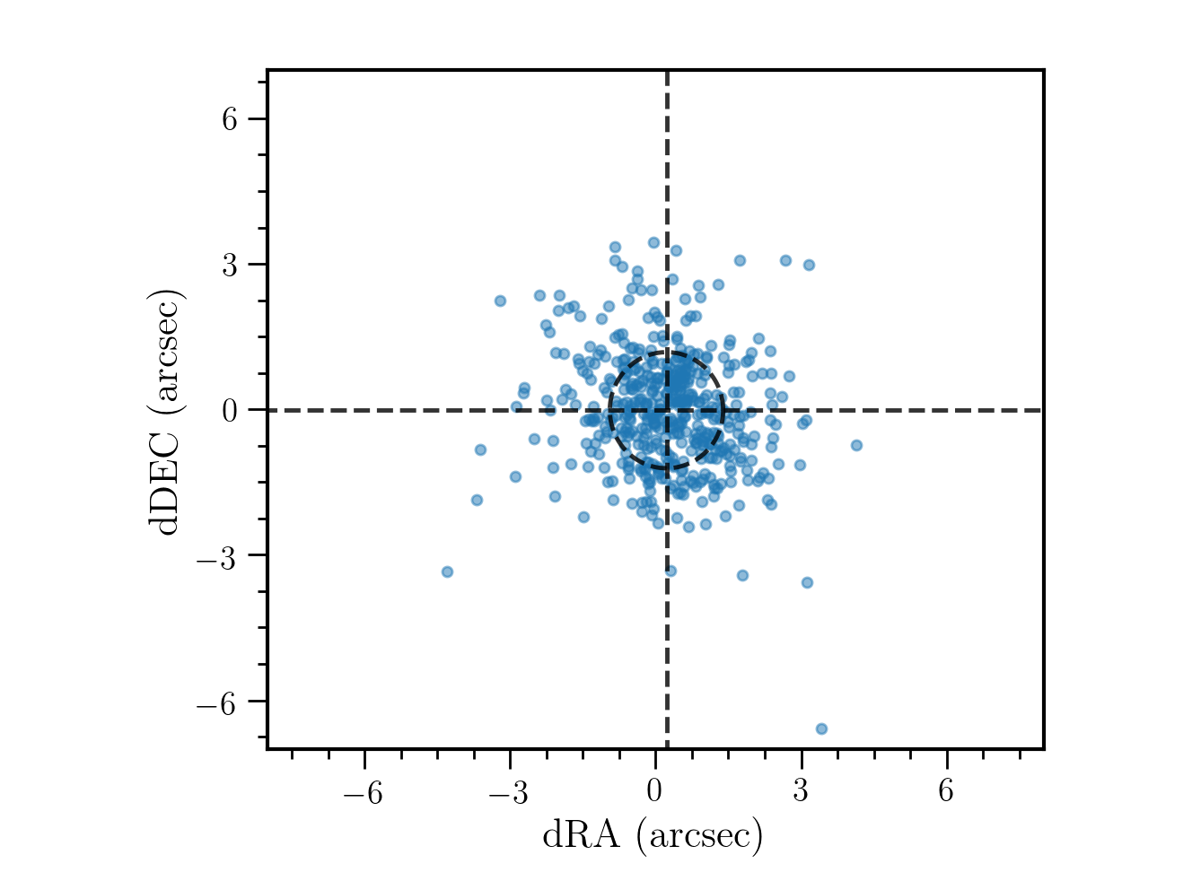
Figure 7: Positional offsets between LBA and deep HBA sources. The oval shows the standard deviation of the distribution in the RA and Dec directions, where the offsets are defined as $dRA=\alpha_{\mathrm{LBA}}-\alpha_{\mathrm{HBA}}$ and $dDEC=\delta_{\mathrm{LBA}}-\delta_{\mathrm{HBA}}$, respectively.

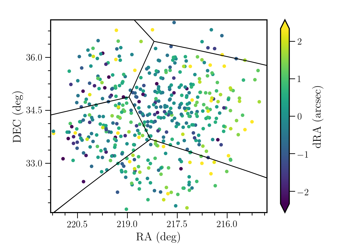
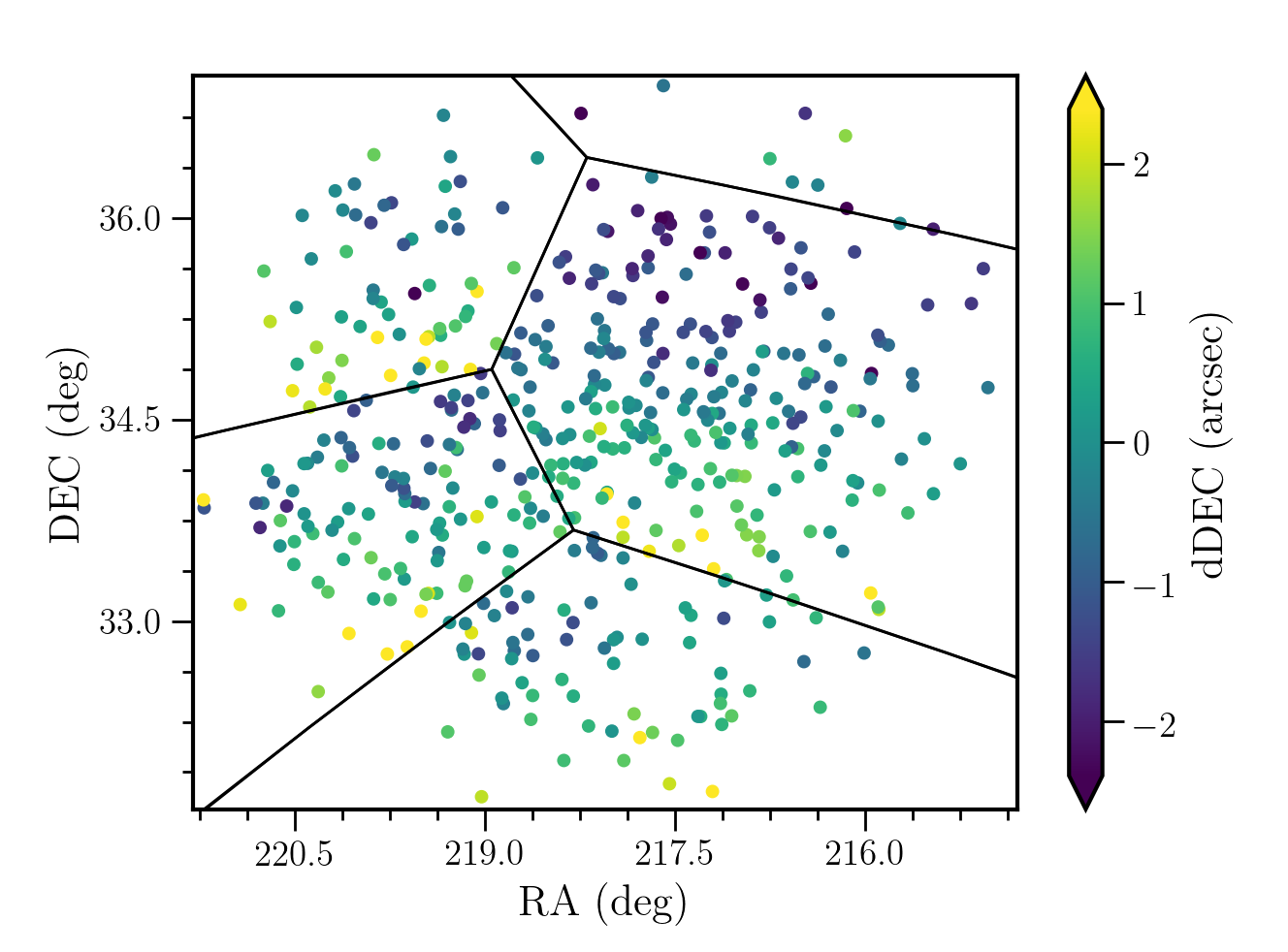
Figure 8: Positional offsets between LBA and deep HBA sources in right ascension, $dRA=\alpha_{\mathrm{LBA}}-\alpha_{\mathrm{HBA}}$, (top) and declination, $dRA=\delta_{\mathrm{LBA}}-\delta_{\mathrm{HBA}}$, (bottom) as a function of position on the sky. The black polygons show the facets used in the calibration and imaging.

4.2 Smearing

By plotting the ratio of the total flux density to the peak intensity (see Fig. 9), it is apparent that there is some level of smearing in that this ratio exceeds unity for almost all sources. For unresolved sources, this ratio should be scattered around unity. The median ratio for small ($<30$  arcsec) single-Gaussian sources increases as a function of distance from the pointing centre, from around $1.5$ at the centre to $\sim 2$ at a radius of $2.5$ degrees. As DDFacet is able to account for a varying psf due to bandwidth and time-averaging during deconvolution, and all these sources are deconvolved, this is likely a result of imperfect phase calibration applied over the very large facets (see Fig. 4). As the facets are large and spread from the centre to the edges of the field, the phase solutions are most applicable in the direction of the greatest apparent flux density of sources which is towards the centre of the field.

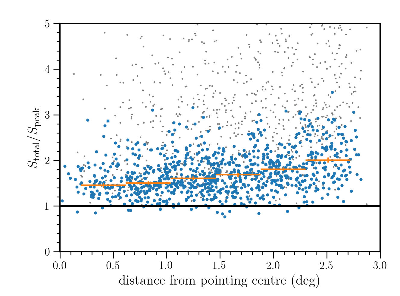
Figure 9: Measured ratio of integrated to peak flux density as a function of distance from the pointing centre for all sources (in gray) and for a selection of compact sources (in blue). The orange crosses show the median smearing of compact sources, which is systematically greater than unity and increases with radius, likely because of imperfect calibration.

4.3 Completeness

To assess completeness, we performed a Monte-Carlo simulation in the image plane in which we generated $25$ random fields each containing approximately $7000$ randomly positioned point sources with flux densities between $2$ and $200$ mJy. The source flux densities were drawn randomly from the $150$-MHz source count distribution of Mandal et al. (2021), scaled to $54$ MHz assuming an average spectral index of $-0.8$. To simulate the effect of smearing, we increased both the major- and minor-axes of these injected 2D Gaussians by $\sqrt{S_{f}}$, where $S_{f}$ is the median smearing factor as a function of distance from pointing centre (see Fig. 9). Sources were added to the residual image produced by the original source detection with PyBDSF. For each simulated image, sources were detected with the same PyBDSF parameters as those described in Section 4, but using the original rms image because this more accurately captures the increased noise level around real bright sources in the image by decreasing the box size used for determining the rms. In each field, approximately $1500$ of the simulated sources were detected.

For each simulated image, we determined the fraction of sources detected as a function of flux density (shown in Fig. 10). Sources are considered detected by matching their coordinates with the injected source catalogue. Only about $250$ sources in each field satisfy the detection criterion of peak intensity $>5\sigma$. Due to the smearing, the detected fraction in the simulations deviates from the fraction of point sources that would be detected based purely on the fraction of the rms below a given value. The completeness, that is, the fraction of recovered sources above a given flux density, is also shown in Fig. 10. This indicates that the catalogue covering the full field is around 90% complete at a flux density of $10$ mJy, while that covering the deep optical area is around 90% complete at a flux density of $6.5$ mJy.

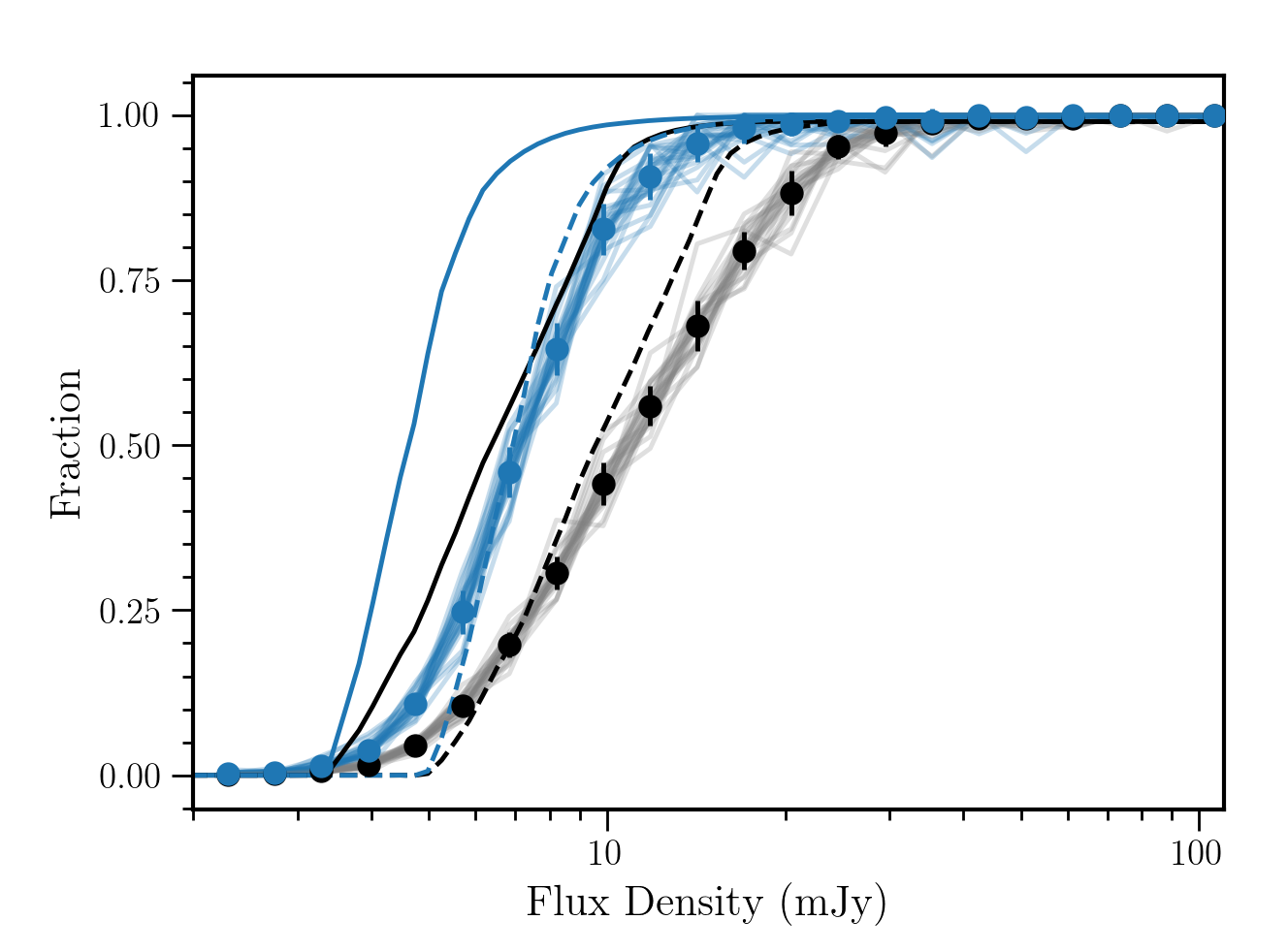
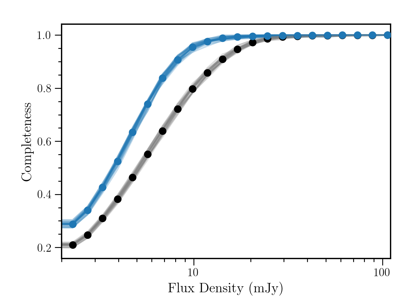
Figure 10: Top: Fraction of simulated sources detected as a function of flux density for each simulated image (in grey) and the median binned points (in black). The solid black line shows the fraction of sources that could be detected with a $5\sigma$ peak intensity threshold based on the rms only, while the dashed black line shows the same but assuming a single average smearing factor of $1.5$, most applicable for the center of the field. The blue points and lines show the same, but determined only over the area with deep optical coverage. Bottom: Estimated completeness above a given flux density —assuming the 150-MHz source count distribution of Mandal et al. (2021)— scaled to $54$ MHz assuming an average spectral index of $-0.8$. This is estimated for the full field (shown in grey and black), and for the region of deep optical coverage (shown in light and solid blue).

4.4 Flux density scale

Given the uncertainties in the low-frequency flux density scale (e.g. Scaife & Heald, 2012, hereafter SH12) and the LOFAR station beam models, we may expect some systematic errors in the measured LOFAR flux densities. In this section we evaluate the uncertainties in the measured LOFAR flux densities and make corrections to the catalogue to account for systematic effects and ensure that the flux densities are on the SH12 flux density scale.

We followed the method of Sabater et al. (2021) to investigate any flux density scale offset, and cross-matched the LBA catalogue with multiple catalogues at higher frequencies, including only relatively compact and isolated sources for the comparison. The flux density measurements from the literature have been adjusted to bring them on to the SH12 scale adopted here, which was designed to be more accurate than previous scales at frequencies below $\sim 300$ MHz. The SH12 scale was calibrated using data on the Roger et al. (1973) flux density scale, which is consistent with the Kellermann et al. (1969) scale above $300$ MHz. Data from the 1.4-GHz VLA surveys —NVSS and FIRST— are on the Baars et al. (1977) flux density scale, and so we used their correction factor (cf. table 7 of Baars et al., 1977) to align the flux densities of these catalogues with the Kellermann et al. (1969) scale. The 1.4-GHz WSRT data were corrected based on NVSS and so we applied the same correction factor. The RACS data are on the Reynolds (1994) flux density scale. This is consistent with the Baars et al. (1977) flux density scale and therefore we used their correction factors (interpolated to 888 MHz from their Table 7) to align the RACS flux densities with the Kellermann et al. (1969) scale. The $325$-MHz data are somewhat more complicated: the correction factor to scale data from WENSS to the SH12 flux scale is an average correction across the discrete set of WENSS calibrators (3C 48, 3C 147, 3C 286 and 3C 295), but this should not apply to localised regions of the sky. As the Boötes field is only 18 deg from 3C 295, it is likely that this is the calibrator that was used for this part of the sky. We therefore scaled the WENSS flux densities by the offset for 3C 295. The 325-MHz VLA data were corrected to the WENSS flux density scale, but we further applied the additional offset factor of 0.95 found by Coppejans et al. (2015). The deep 150-MHz data were corrected by the factor determined by Sabater et al. (2021). The flux densities of the remaining catalogues were all calibrated with respect to SH12 or Roger et al. (1973), and so no further corrections were made. Table 3 lists all the catalogues used with their flux scale corrections and the details of the cross-matching selection to select only compact isolated sources. For the catalogues that are much deeper, we considered only the brighter sources to avoid any bias from a changing spectral index at lower flux densities (see Sect. 5.2). Following the method of Sabater et al. (2021) we set flux density thresholds for both of the cross-matched surveys to avoid a bias towards sources with high absolute values of their spectral indices. For each catalogue, we calculated the ratio of the catalogued flux densities to those at $54$ MHz. The median of this ratio is plotted in Fig. 11. The straight line fitted to these ratios gives a value at $54$ MHz of $0.96\pm 0.11$, suggesting that the LBA catalogued flux densities are consistent with unity. We therefore apply no correction to the catalogued flux densities.

Table 3: Catalogues and cross-match parameters used to test the flux density scale

Catalogue	Frequency	Size Limit	Resolution	Match radius	Flux Limit	Flux scale correction	Flux scale error	Flux Ratio	Reference
	(MHz)	(arcsec)	(arcsec)	(arcsec)	(mJy)
LOFAR60	62	60	30	30	1	1	0.2	$0.962_{0.193}^{0.195}$	1
VLSSr	74	30	75	75	530	1	0.2	$0.787_{0.159}^{0.170}$	2
6C	151	30	60	60	250	1	0.2	$0.517_{0.106}^{0.105}$	3
LOFAR150	150	60	7.5	15	0.01	1	0.15	$0.463_{0.070}^{0.070}$	4
T-RaMiSu	153	30	25	15	10	1	0.15	$0.503_{0.078}^{0.076}$	5
LOFAR150-DEEP	144	60	6	6	10	0.859	0.1	$0.450_{0.045}^{0.046}$	6
VLA-P	325	30	5.5	15	2	0.935	0.15	$0.319_{0.048}^{0.050}$	7
WENSS	325	60	30	30	15	0.982	0.15	$0.250_{0.038}^{0.038}$	8
GMRT610	610	30	5.5	5.5	2	1	0.15	$0.207_{0.038}^{0.036}$	9
RACS	888	30	25	15	2	1	0.15	$0.207_{0.038}^{0.036}$	10
WSRT1400	1400	60	54	54	1	1.029	0.1	$0.100_{0.012}^{0.013}$	11
NVSS	1400	60	45	45	2	1.029	0.1	$0.092_{0.010}^{0.010}$	12
FIRST	1400	30	5	15	2	1.029	0.1	$0.091_{0.010}^{0.010}$	13

(1) van Weeren et al. (2014); (2) Lane et al. (2014); (3) Hales et al. (1988); (4) Williams et al. (2016); (5) Williams et al. (2013); (6) Tasse et al. (2021); (7) Coppejans et al. (2015); (8) Rengelink et al. (1997); (9) Coppejans et al. (2016); (10) McConnell et al. (2020); (11) de Vries et al. (2002); (12) Condon (1997); (13) Becker et al. (1995).

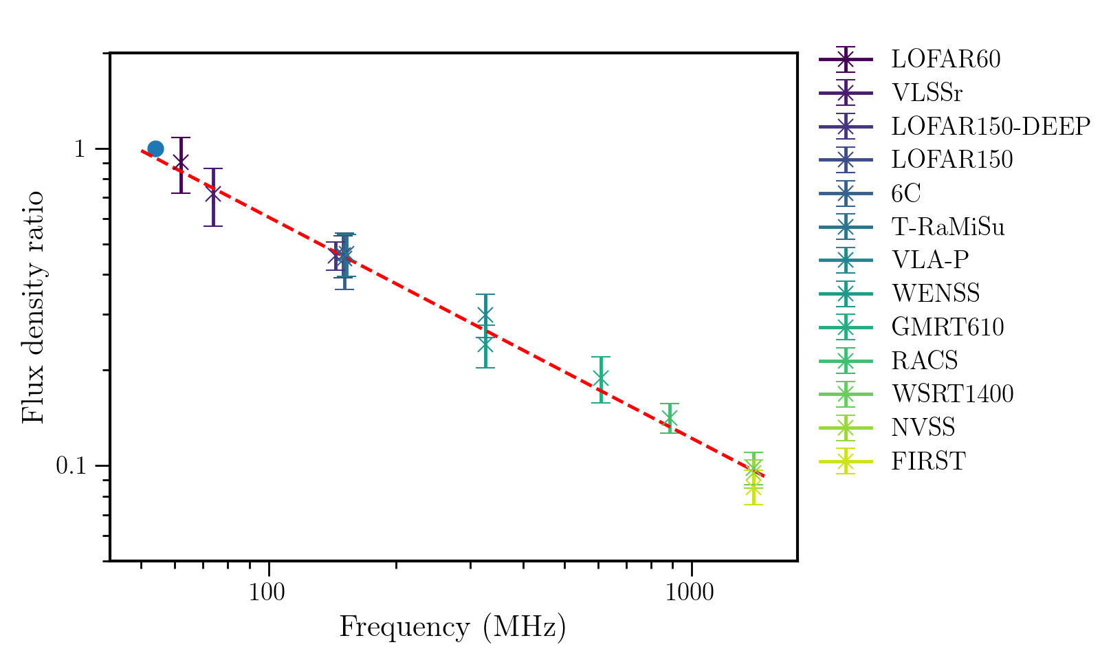
Figure 11: Flux density scaling predicted from observations at multiple frequencies compared to that observed at $54$ MHz here.

We also checked for any variation in the total flux density ratio with distance from the phase centre or position on the sky and found none. The ratio between the $54$-MHz and $144$-MHz flux densities is shown as a function of sky position in Fig. 12 for a sample of bright ($S_{54\mathrm{MHz}}>20$ mJy), high-signal-to-noise-ratio ($S/N>7.5$), and small ($<30$  arcsec) sources. Here, the $144$-MHz flux densities from the deep HBA image have been scaled to $54$ MHz with an assumed spectral index of $-0.7$. There is no noticeable trend with position.

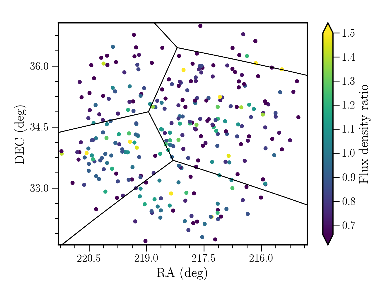
Figure 12: Ratio of flux density at $54$ MHz and the scaled $144$-MHz flux density as a function of position on the sky. The black polygons show the facets used in the calibration and imaging.

5 Spectral indices and source counts

The $1,948$ sources in the catalogue provide a statistically significant sample across three orders of magnitude in flux density from $3$ mJy to $18$ Jy. The addition of the deep $144$-MHz data available allows the calculation of spectral indices for all sources in the catalogue. In this section we present the derived spectral index distributions and 54-MHz source counts.

5.1 HBA cross-matching

Through a process of visual inspection we matched the LBA sources with those from the deep $144$-MHz HBA image (Tasse et al., 2021), which has a central noise level of $30$ $\mu$Jy beam^-1. Within the area of deep optical coverage, we performed the cross-match against the catalogue of Kondapally et al. (2021), which includes the optical identifications as well as the restructuring of the raw PyBDSF source catalogue from Tasse et al. (2021) into true physical sources. In this process, following that of Williams et al. (2016) and Kondapally et al. (2021), we decomposed some of the LBA PyBDSF sources into their Gaussian components and (re-)combined some PyBDSF (Gaussian components) sources into final physical sources. We also flagged some PyBDSF sources as artefacts. The resulting matched catalogue contains $1,789$ sources —of which $829$ ($46$ per cent) lie within the deep optical coverage— and is available online¹¹. The much greater depth of the HBA data (about 50 times greater for a source of spectral index $-0.7$) means that all the LBA sources are detected in the HBA image; a source with a $54$-MHz flux density of $5$ mJy would have to have a spectral index steeper than $-2.5$ to be undetected at $144$ MHz and there are no such sources in the field.

5.2 Spectral Indices

The spectral indices, $\alpha_{54}^{144}$, calculated for these matched sources are plotted in Fig. 13 as a function of their HBA flux densities. The greater depth of the HBA data means that the faintest HBA sources also detected at $54$ MHz preferentially have steeper spectra, that is, the faintest HBA sources with flatter spectra fall below the detection limit of the LBA. This incompleteness is indicated by the shaded grey areas in Fig. 13 where sources within the darkest region cannot be detected and those within the lighter region may only be detected in part of the LBA image. We therefore only calculate the median spectral indices in bins above 144-MHz flux densities of $5$ mJy beam^-1. Nevertheless, there is a clear trend towards flatter spectral indices with decreasing $144$-MHz flux density, from $\sim-0.75$ at flux densities between $100$ and $1000$ mJy to $\sim-0.5$ at flux densities between $5$ and $10$ mJy.

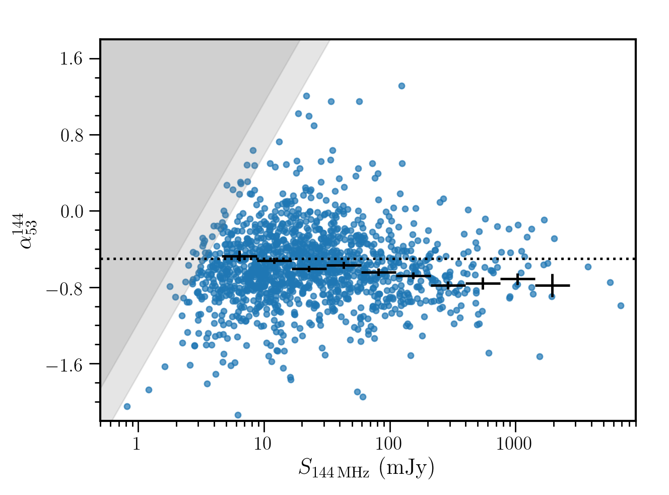
Figure 13: Spectral indices measured between $54$ and $144$ MHz with LOFAR LBA and HBA respectively. The grey shaded areas show where the distribution becomes incomplete for flatter sources due to the varying sensitivity of the LBA observations, assuming a $5\sigma$ detection of a point source at the minimum ($0.65$ mJy beam^-1, light grey) and median ($1.1$ mJy beam^-1, dark grey) rms. The dotted line shows a value of $-0.5$ to guide the eye. The black points show the median values and errors on the median within equally spaced logarithmic flux-density bins, showing a flattening of spectra towards lower flux densities.

Using the optical identifications (Kondapally et al., 2021) and source classifications (Best et al. in prep) available for the deep HBA sources, we investigated the spectral indices for AGN and SFGs separately. Of the $829$ LBA sources within the deep optical coverage, $61$ are classified as SFGs, while $626$ are classified as radio-loud AGN, and $29$ as radio-quiet AGN. A further $113$ are unclassified. These fractions are broadly consistent with predictions from the SKA simulated skies models (SKADS Wilman et al., 2008), which yield about $30$ SFGs and about $800$ AGN taking into account the varying rms and masked deep optical area. The differences may be a result of different models used within SKADS or the SFG/AGN classification used by Best et al. (in prep) which relies on the radio excess above the far-infrared radio correlation. The spectral indices for the SFGs and radio-loud AGN are shown in Fig. 14, and again only showing the median spectral indices in $144$-MHz flux density above $5$ mJy beam^-1, where the median values are not affected by the incompleteness. The majority of the sources are classified as AGN (both high excitation and low excitation radio galaxies) with SFGs only appearing at lower flux densities, but it is apparent that the SFGs have flatter radio spectra. The median spectral index for the SFGs is $-0.4$. This is consistent with a further flattening of the spectra of SFGs compared to that found by Calistro Rivera et al. (2017) at higher frequencies where the average spectral index of SFGs between $150$ and $325$ MHz was found to be $-0.6$ while that between $325$ and $1400$ MHz was a steeper $-0.78$ due to free-free absorption at the lower frequencies (see also Ramasawmy et al., 2021).

The flattening of the spectral index towards lower flux densities is also evident in the AGN population. With the size information from the higher resolution HBA data, we consider the spectral indices of the AGN for about $150$ compact sources, defined as having a deconvolved size of $<2$  arcsec, and for about $320$ extended sources of $\geq 2$  arcsec. This is shown in Fig. 15, from which it is apparent that the compact sources have flatter median spectral indices at lower flux densities compared to the more extended sources, which remain steep ($\alpha^{144}_{54}\sim-0.7$). This is similar to the result of de Gasperin et al. (2018a) who found a similar trend in the spectral index between $150$ MHz and $1.4$ GHz with both flux density and source compactness. This is likely because the population of large sources is dominated by lobe-dominated sources, where more synchrotron emission comes from old electron populations and is thus steeper. The overall flattening of the spectral indices at lower flux densities is therefore likely driven by a growing population of SFGs and core-dominated, compact AGN.

Figure 14: Spectral indices measured between $54$ and $144$ MHz, with LOFAR LBA and HBA respectively. Grey points show all matched sources, while the coloured points show those within the optical coverage, where sources have been classified as SFGs (blue) or AGN (orange). The large coloured points show the median values and errors on the median within equally spaced logarithmic flux density bins for the two populations separately.

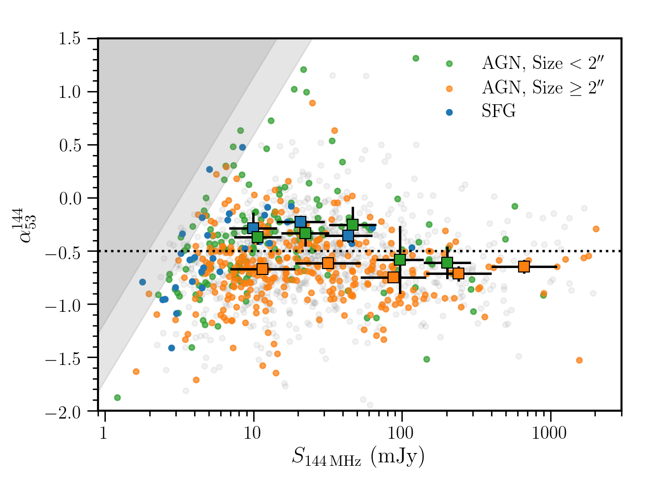
Figure 15: As in Fig. 14, but only the AGN are plotted and are plotted separately for extended (orange) and compact (green) sources, where the source size is determined from the 144 MHz data.

5.3 Source counts

The Euclidean-normalised differential source counts for this catalogue are plotted in Fig. 16, where we show both the raw counts and those corrected for completeness using the results of Fig. 10. The errors on the raw counts per flux density bin are the Poisson errors corrected for small numbers (Gehrels, 1986). The primary causes of incompleteness are the varying rms level due to the ‘primary’ beam (see Fig. 6) and the residual ionospheric smearing (see Sect. 4.2). To account for this, we used the detection fraction (see Fig. 10) determined from the completeness simulations to correct the raw source counts. Errors on the final counts are propagated from the errors on the detection fraction from the simulations. The source counts presented here were determined using the full image, but agree with those determined only within the area of deep optical coverage or within $1$ degree of the phase centre, where the smearing is less dominant and the completeness is higher. It should be noted that the lowest flux-density bins are determined from sources only found in the central region ($\lesssim 3$ deg²), and so they may be affected by cosmic variance. Following the method outlined by Prandoni et al. (2001) and Williams et al. (2016), we make a correction for the resolution bias, that is, the preferential non-detection of large sources, which takes into account the size distribution of sources. This correction is much smaller than the completeness correction. The counts presented here complement the LoLSS source counts (de Gasperin et al., 2021), which provide better statistics at the brighter end, while our deep-field counts probe the fainter sources where LoLSS becomes incomplete.

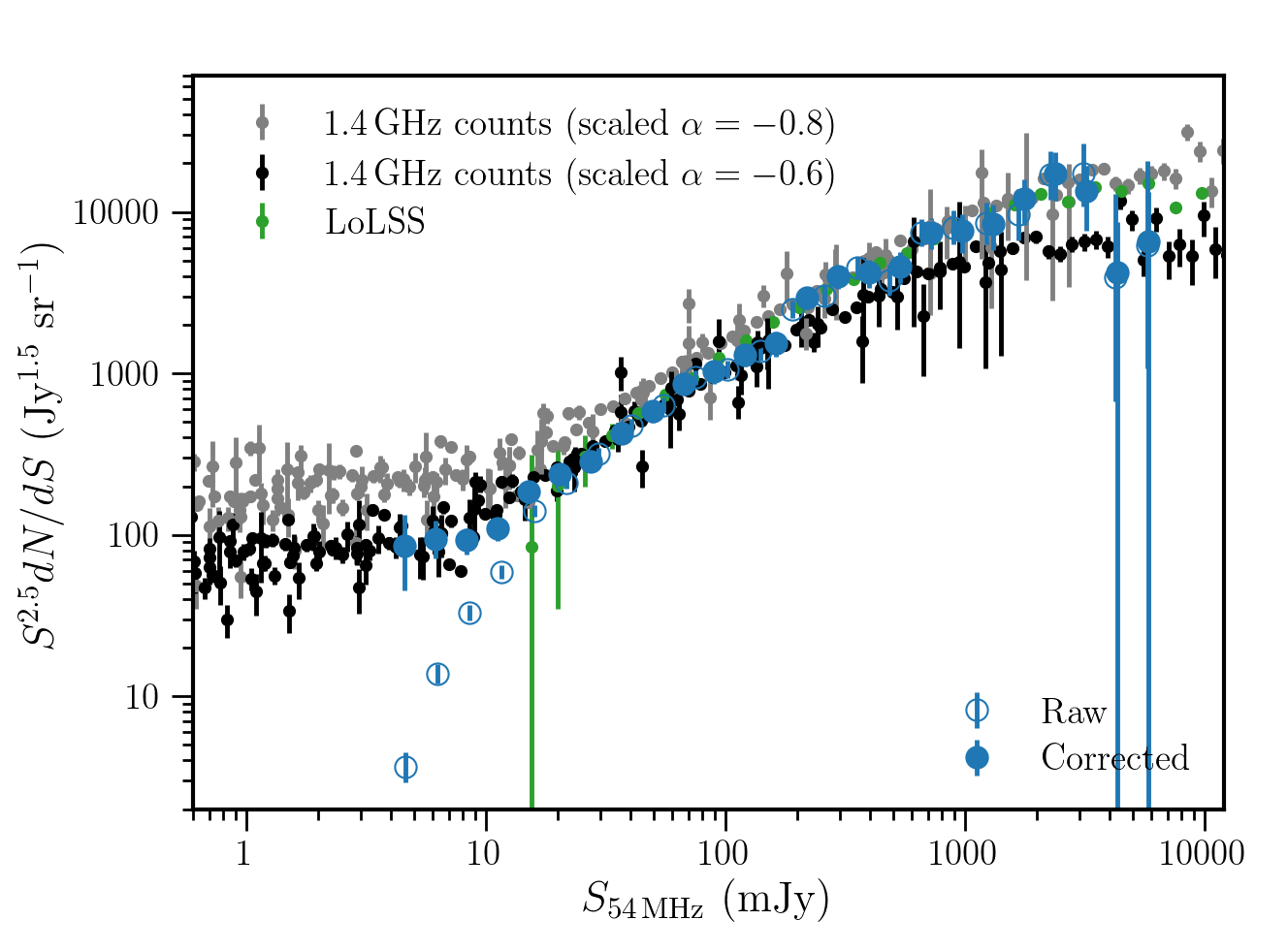
Figure 16: Euclidean-normalised differential source counts for the Boötes field between 4 mJy and 7 Jy. The open circles show the raw, uncorrected source counts, while the filled circles show the completeness-corrected counts. For comparison we include the $1.4$ GHz source counts from various surveys compiled by de Zotti et al. (2010), Bonato et al. (2017), and Bonato et al. (2021), and scaled to $54$ MHz assuming a spectral index of $-0.8$ (in gray) and $-0.6$ (in black), and the $54$-MHz LoLSS source counts between 10 mJy and 30 Jy (small green points).

We compared the Euclidean-normalised source counts derived here with the compilations of $1.4$ GHz source counts by de Zotti et al. (2010), Bonato et al. (2017), and Bonato et al. (2021). We find very good agreement with the higher-frequency counts if we assume different spectral indices at different flux densities. There is some deviation in the lowest flux density bin $4$–$5$ mJy, which may be a result of incompleteness. An average spectral index from $-0.8$ works well at $54$-MHz flux densities above $\sim 100$ mJy, while an average spectral index of $-0.6$ works well at lower flux densities. This is consistent with the change in the measured median spectral indices of individual sources both in this work (see Sect. 5.2) and that of de Gasperin et al. (2018a).

In five flux density bins we determined the spectral index that provides the best scaling between the $1.4$-GHz and $54$-MHz source counts. This is plotted in Fig. 17, where we include the flux-density-dependent spectral index from Fig. 13. Again this shows the flattening of the spectral index towards lower flux densities, but in a statistical way, for the radio source populations at these two frequencies. This flattening is consistent with that observed between 54 MHz and 144 MHz for sources matched individually. There is some indication that at $S_{54\mathrm{MHz}}\sim 10$ mJy the radio spectra at $54$–$144$ MHz are flatter than at $54$–$1400$ MHz suggesting curvature in the spectra of these sources. However, this may be due to the residual incompleteness in the $54$-MHz source counts and warrants further investigation with deeper LBA observations, and detailed follow-up multi-frequency studies of the spectra of individual sources.

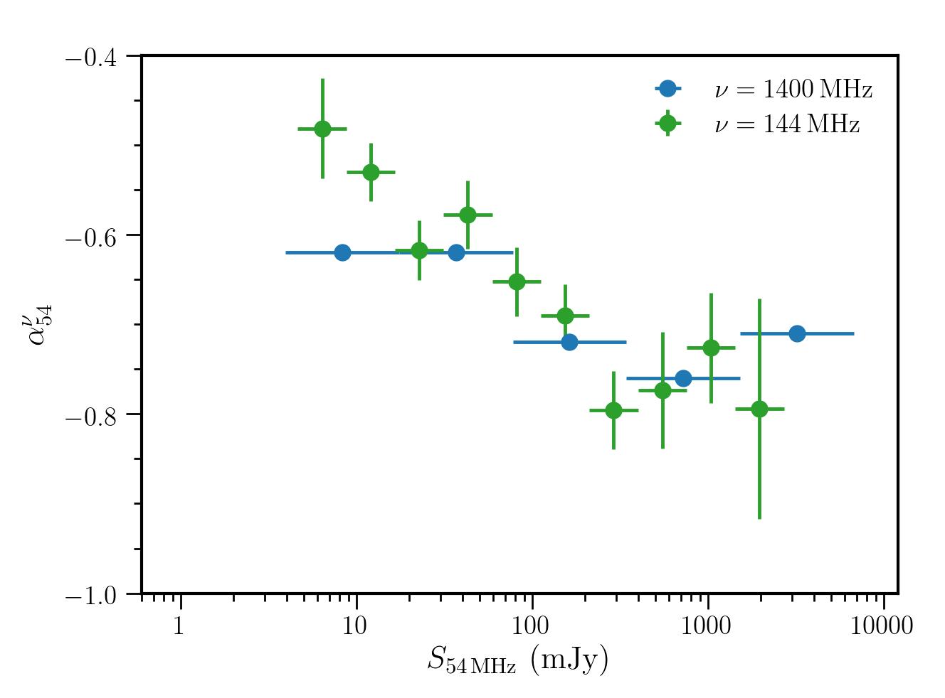
Figure 17: Average spectral index of all sources between $1.4$ GHz and $54$ MHz determined from the source counts (in blue), and between $144$ MHz and $54$ MHz determined from individual sources (from Fig. 13, in green).

6 Summary

We present the first deep ($\approx 0.7$ mJy beam^-1), high-resolution ($15\times 15$ arcsec) LOFAR LBA image of the Boötes field made at $34$–$75$ MHz from $56$ hours of observation and describe the full data reduction process from observations to the direction-dependent calibrated image. The radio source catalogue of $1,289$ sources over an area of $23.6$ deg² allows us to characterise the low-frequency radio source population with unprecedented sensitivity. We present the Euclidean-normalised source counts and investigate the spectral indices of the source population, both of which indicate a flattening of the low-frequency radio spectra of fainter radio sources.

Our observations show that sub-mJy noise levels are obtainable with deep observations at these frequencies. Additional observations of this field and other fields as part of LoLSS-Deep will allow us to probe even deeper, and to increase the area covered to provide better source statistics. Since the time of the observations presented here, a number of improvements have been made in the LOFAR LBA station calibration, resulting in improved sensitivity. Further improvements in calibration are underway and will improve the imaging quality, particularly the dynamic range limitations around bright sources and the residual ionospheric smearing.

The combination of the very deep HBA data available for the Boötes deep field and the wealth of multi-wavelength data, including redshifts and source classifications, will allow further detailed studies of the spectral properties of both star-forming galaxies and AGN.