Gallego and Berbeglia

Bounds, Heuristics, and Prophet Inequalities

Bounds, Heuristics, and Prophet Inequalities for Assortment Optimization

Guillermo Gallego School of Data Science, Chinese University of Hong Kong in Shenzhen gallegoguillermo@cuhk.edu.cn Gerardo Berbeglia Melbourne Business School, The University of Melbourne, Australia g.berbeglia@mbs.edu

Abstract: We introduce odds-ratios in discrete choice models and utilize them to formulate bounds instrumental to the development of heuristics for the assortment optimization problem subject to totally unimodular constraints, and to the assess the benefit of personalized assortments. These heuristics, which only require the first and last-choice probabilities of the underlying discrete choice model, are broadly applicable, efficient, and come with worst-case performance guarantees. We propose a clairvoyant firm model to assess, in the limit, the potential benefits of personalized assortments. Our numerical study indicates that when the mean utilities of the products are heterogeneous among the consumer types, and the variance of the utilities is small, then firms can gain substantial benefits from personalized assortments. We support these observations, and others, with theoretical findings. For regular DCMs, we show that a clairvoyant firm can generate up to $n$ times more in expected revenues than a traditional firm. For discrete choice models with independent value gaps, we demonstrate that the clairvoyant firm can earn at most twice as much as a traditional firm. Prophet inequalities are also shown to hold for a variety of DCMs with dependent value gaps, including the MNL and GAM. While the consumers’ surplus can potentially be larger under personalized assortments, clairvoyant firms with pricing power can extract all surplus, and earn arbitrarily more than traditional firms that optimize over prices but do not personalize them. For the price-aware MNL, however, a clairvoyant firm can earn at most $\exp(1)$ more than a traditional firm.

prophet inequalities, assortment optimization, revenue-ordered assortments The first version of this paper was uploaded to ArXiv in September 2021.

1 Introduction

Two key problems faced by assortment managers are (1) how to find optimal or near-optimal assortments subject to certain business constraints and (2) whether or nor to personalize assortments. The aim of this paper is to tackle these two problems by studying properties about the first and last-choice probabilities of the underlying aggregate discrete choice model (DCM) based on multinomial logit (MNL) approximations.

The Traditional Assortment Optimization Problem (TAOP) is in general NP-hard, and even versions that are polynomially solvable often become NP-hard when firm needs to satisfy some constraints (Sumida et al. 2021, Désir et al. 2020). Many business constraints can be represented as totally unimodular (TUM) constraints. Two examples of TUM constraints are cardinality constraints and precedence (or conditional) constraints, where a product can only be shown if another product is offered. While there exist efficient methods to solve TAOP with TUM constraints for very simple choice models, little is known about the performance of fast methods to solve this problem for more realistic choice models. In this paper we will show how to approximate regular DCMs by tractable models based on first-choice and last-choice probabilities. These approximations are then used to develop heuristics and in some cases provide easy to compute performance guarantees.

The issue of personalization is particularly important in a context where companies have access to more information about its customers. The problem of personalizing assortments is important to business, to consumers and to government regulators. Moreover, its relevance is increasing as online retailers take a higher market share of all sales, reducing the market share of traditional brick-and-mortar counterparts. Assortments offered by brick and mortar stores are of a more strategic nature as they are designed to show the products in an attractive way and to lure consumers into the store. Changing the offered assortment requires reorganizing the store and to have a backroom to hide the products that the store currently does not desire to offer. In contrast, an online platform can make instant changes depending on the information it gathers about consumers. The platform may gather information about the consumers’ location and search keywords and then decide what products to display in real-time. This has led online firms to create consumer types based on such information and solve an assortment optimization problem for each segment. Several papers addressed personalized assortment optimization policies and study their benefits and limitations e.g. Golrezaei et al. (2014), Bernstein et al. (2015), El Housni and Topaloglu (2023). As e-commerce firms collect more detailed personal information about web searches, click-through paths and past purchases, they become more able to create segments of size one and truly offer personalized assortments and personalized prices. This has raised the concern of public and policy makers (see, Tucker (2014), Goldfarb and Tucker (2012)) and to welfare studies of personalized assortments and personalized pricing (see e.g. Ichihashi (2020)).

Firms and policy makers are interested in understanding the impact of personalization when it is taken to a very high degree. In this paper we take a step in this direction by introducing a clairvoyant firm that manages to sell to each arriving consumer the highest revenue product that they are willing to buy and ask how much more a clairvoyant firm can make relative to a TAOP-firm. Although firms may never develop the power to read consumer minds, the analysis of this extreme case is useful since it provides a quantifiable limit to the firm’s benefits of doing any personalization strategy. Moreover, the resulting upper bounds are elegant, tight, and, for some families of choice models, only a constant factor away from the revenue of a TAOP-firm, and in some cases a constant away form the revenue-ordered heuristic. In our studies we find that the consumer’s surplus may be larger under the clairvoyant firm than under the TAOP firm. This suggests that regulators need to be extremely carefully in regulating personalized assortments.

1.1 Our Contributions

We divide our contributions into four themes.

• New heuristics for assortment optimization: We introduce the notion of the odds-ratio for regular choice models and leverage bounds on the odds-ratios to develop a new heuristic approach for the constrained Traditional Assortment Optimization Problem (TAOP) with totally unimodular (TUM) constraints. Our heuristic approach is very general (e.g. it works for any regular choice model) and fill a void as little is known on how to handle problems with TUM constraints for regular choice models. While these heuristics are not conceived to compete with heuristics specifically designed for sub-families of choice models and particular TUM constraints, they typically capture a large fraction of the revenue obtained by the specialized heuristics, run faster, and in some cases have explicitly computable performance guarantees. Additionally, these heuristics require very little information about the choice model, namely first and last-choice probabilities, and as a result they can be extremely useful in real world settings where model parameters aren’t fully known.

• Clairvoyant firm in assortment optimization: To explore the limits of personalization, we introduce a clairvoyant firm that sells to each arriving consumer the highest revenue product she is willing to buy. We demonstrate that the expected revenue of a clairvoyant firm serves as an upper bound on the expected revenue achievable by any personalized policy. Perhaps surprisingly, in Theorem 3.1 we show that under mild conditions, the expected revenue of a clairvoyant firm can be easily computed with the mere knowledge of the outside alternative probabilities for revenue-ordered assortments. Furthermore, in Theorem 3.2 we establish upper bounds on the revenue achievable by the clairvoyant firm, relying solely on the vector of last-choice probabilities. Building on these results, we conduct a numerical study that examines the bounds of personalization in randomly generated latent-class Mixed Logit (MNL) models. These results suggest that the most advantageous scenarios for personalization are those where the firm possesses knowledge of the underlying MNL model for each consumer type, the coefficient of variation of the utilities is small, and there is sufficient spread in the mean utilities across consumer types. This is consistent with our intuition as then knowing the type carries significant information. On the other hand, for instances with low heterogeneity in the means and high variance in the utility the benefits of personalization become small or negligible. These insights are later confirmed by analytical observations and Theorem 3.3. We have also examined extreme cases and discover intriguing results. First, we demonstrate that for regular Discrete Choice Models (DCMs), a clairvoyant firm has the potential to earn up to $n$ times more revenue than a TAOP firm, where $n$ represents the number of products available. Remarkably, this bound is tight and there is a personalized policy that earns as much as the clairvoyant firm. Moreover, the result remains true even when considering the restricted setting of the Markov chain choice model (Theorem 3.4). At the other end of the spectrum, when the DCM is governed by the independent choice model, a clairvoyant firm can make no more than a traditional firm that does not personalize assortments (Proposition 3.5). We also show that offering products sequentially in descending order of revenue can achieve revenue on par with a clairvoyant firm for consumers who adhere to a persistent and satisfying policy. This policy entails consumers purchasing the first satisfying product they encounter and continuing their search until they find a product they like or run-out of products (Proposition 3.6).

• Prophet Inequalities for Assortment Optimization:

  We first investigate DCMs with independent value gaps, and demonstrate the validity of the well-known prophet inequality, indicating that a clairvoyant firm can generate at most twice the revenue of a TAOP firm (Proposition 4.1). Models with independent value gaps include the Random Consideration Set (RCS) model, and the random utility model with deterministic utility for the outside alternative. Moreover, we present a series of results showcasing that the prophet inequality holds for various models with dependent value gaps, including the Multinomial Logit (MNL), the Generalized Attraction Model (GAM), and a non-standard Nested Logit (NL) model, among others (Theorems 4.2, 4.3, and 4.6, and Corollary 4.4 and Proposition 4.5). These findings highlight the implications of the prophet inequality in different model frameworks.

• Extensions: In the discussion section, we provide additional results that relate to recent papers on refined assortment optimization (Berbeglia et al. 2021b) and joint assortment and customization (El Housni and Topaloglu 2023). These results offer refinements of earlier results with new bounds provided by the clairvoyant firm. Furthermore, we delve into the realm of clairvoyant pricing and explore its implications. Specifically, we demonstrate that a clairvoyant firm with the ability to customize its prices has the potential to earn arbitrarily more revenue than a TAOP firm (Propositon 5.1), highlighting the significant advantage of perfect information coupled with pricing freedom. However, for the Multinomial Logit (MNL) model, we establish that a clairvoyant firm that can customize the prices to each incoming consumer can make up to $e\approx 2.71828$ times more revenue with respect to a firm that must treat all consumers equally (Proposition 5.2).

1.2 Related literature

The literature on assortment optimization has increased dramatically during the last 15 years starting with the seminal paper of Talluri and Van Ryzin (2004) where the authors assume that consumer preferences can be described by an MNL model. Reviews of the subject can be found in Strauss et al. (2018), Den Boer (2015), Lobel (2021), and the recent book by Gallego and Topaloglu (2019). The assortment optimization problem has been studied under different choice models (see, e.g. Blanchet et al. (2016) and Davis et al. (2014)). In addition, it has also been studied in different settings such as where the firm faces cardinality limitations on the offer sets and similar constraints (see e.g. Rusmevichientong et al. (2010), Désir et al. (2020), Sumida et al. (2021)) and in settings where inventory is limited (see e.g. Topaloglu (2009)). Recently, there has been an interest in understanding the limitations of traditional assortment optimization and assessing the benefits of enlarging the possible actions taken by the firm such as using lotteries (Ma 2022), reducing product utilities (Berbeglia et al. 2021b), increasing product advertisement (Wang et al. 2021), and customizing the assortment offered (see e.g. Bernstein et al. (2015) and references in the following paragraph).

While the benefits of personalization has been recognized several decades ago (see, e.g. Surprenant and Solomon (1987)), it is only recently that researchers began to study personalized assortment optimization problems. In these problems, consumers are divided into types, and each type follows a discrete choice model that has residual uncertainty. The objective is to choose a (possibly) different assortment to offer to each segment to maximize expected revenues. One of the earliest works in personalized assortments was carried out by Bernstein et al. (2015) who studied a finite-horizon setting in which consumers follow a mixed MNL model, demand is stationary, and the seller is able to observe the segment class of the incoming consumer. In their model, all products have the same revenue, products are limited in inventory, and the seller must choose a personalized assortment at each period. The authors provide structural results about the optimal policy and develop some heuristics. Chan and Farias (2009) studies a framework that contains the previous model but allows non-stationary demand and different product prices and show that a myopic policy guarantees at least half of the revenue of the optimal control policy. Golrezaei et al. (2014) also extended the model of Bernstein et al. (2015) to non-stationary demand and allowing different prices and proposed a personalized assortment policy that achieves 50 percent of the optimal revenue even against an adversarial chosen demand. The authors showed that the bound is tight. Gallego et al. (2015a) considers a similar model but allows for product revenues to be dependent on the consumer types. The authors propose online algorithms to offer personalized assortments that guarantee a factor of $(1-\epsilon)$ of the optimal offline revenue (under complete information) where $\epsilon$ is the error in computing an optimal solution to the choice based linear program (CDLP). Bernstein et al. (2019) proposes an exploration-exploitation framework to learn consumer preferences and personalize assortments under a finite-horizon. They develop a dynamic clustering estimation algorithm that maps consumer segments to clusters. In a case study, the authors show that the clustering policy increased transactions by more than 37% with respect to learning and treating each consumer type separately. Kallus and Udell (2020), who considers a similar framework, argues that the amount of data required to estimate a LC-MNL model is orders of magnitude larger than the data available in practice. To overcome this issue, they impose that the parameter matrix associated to the LC-MNL has a low rank and showed that the model can be learned quickly. They also showed that an exploration-exploitation algorithm that is rank aware and does assortment personalization has much lower regret with respect to those who ignore the rank structure. Cheung and Simchi-Levi (2017) studies another exploration-exploitation setting in which each consumer follows its own MNL model according to their observable attributes. They develop a Thompson sampling based policy to personalize assortments and prove regret bounds with respect to the optimal policy. Jagabathula et al. (2022) developed algorithms to perform personalized promotions in real-time. The authors consider a choice model in which consumers have a partial order among the products which is combined with an MNL. They develop a MILP which, for an incoming consumer, would personalize the assortment of products offered at a fixed discounted price. Chen et al. (2021) consider a learning problem where a firm uses transactions to personalize prices or assortments. The authors developed a unified logit modeling framework in which products and consumers have a feature vector that lie in a multi-dimensional real space. The nominal value of a product to a given consumer is a linear function of the product and consumer features and the error terms follow a Gumbel distribution. They establish finite-sample convergence guarantees that are later traduced into out-of-sample performance bounds.

A personalized assortment may reveal private customer data about the consumer to third-parties. Recently, Lei et al. (2020) considers the personalized assortment optimization problem when the firm must ensure that the assortment policy doesn’t reveal private information using the differential privacy framework (Dwork 2006). Berbeglia et al. (2021b) provides tight revenue guarantees on the performance of the well-known revenue-ordered assortment strategy with respect to the optimal personalized assortment solution. Their result holds for regular DCMs (which includes all RUMs) and works even under personalized refined assortment optimization where the firm may reduce the product utilities to some consumer types. El Housni and Topaloglu (2023) studies a two-stage personalized assortment optimization problem with capacity constraint under the LC-MNL model. In their model, consumers follow a LC-MNL and the firm is able to observe the segment of the incoming consumer to customize the final assortment offered. After proving that the problem is NP-hard, they developed an efficient algorithm that guarantees $\Omega(\frac{1}{\log(m)})$-fraction of the optimal revenue where $m$ is the number of segments. We strengthen that result and show that the same revenue guarantee holds with respect to a clairvoyant firm (see Section 5.3). More recently, Udwani (2021) provided a (0.5-$\epsilon)$-approximation algorithm for the same problem.

Many researchers have studied settings where the firm can customize product prices. One key advantage of a personalized assortment policy with respect to personalized pricing is that it is easier to implement as there is no need to calibrate a price-aware discrete choice model. In addition, personalized pricing is sometimes banned by law and it is generally perceived as an unfair practice (Haws and Bearden 2006). A personalized assortment strategy can better deal with those issues. For instance, a firm doing personalized assortments may simply personalize the products that appear at a prominent position (e.g. in the first page of results) but allow consumers to see the same set of products if they continue browsing. Although the offer set is actually the same for all consumers, this policy has a similar effect in consumers as personalized assortments (Abeliuk et al. 2016, Gallego et al. 2020, Aouad and Segev 2021, Berbeglia et al. 2021a). The reader interested in personalized pricing is referred to Elmachtoub et al. (2021), Chen et al. (2020) and Gallego and Berbeglia (2021) and references therein. In Section 5.2 we prove that; under the MNL model; a clairvoyant firm who can customize product prices to each consumer can extract up to $e\simeq 2.718$ times more revenue with respect to the firm who must set the same prices to each consumer. Recently, Goyal et al. (2023) consider a different stochastic variant of the assortment optimization problem, where the parameters that determine the revenue and the demand of each item are drawn from some known distribution. While the authors also evaluate the profit of a clairvoyant firm, their setting is very different from ours since the randomness in their case comes from the model parameters (including revenue) and not from the consumer choices.

2 MNL bounds for assortment optimization

In this section we construct heuristics to solve assortment optimization problems with totally unimodular (TUM) constraints for the class of regular discrete choice models (DCMs). Our heuristics require only the first and last-choice probabilities of the underlying (DCM). Under mild conditions the heuristics have worst-case performance guarantees. Computational experiments are presented to assess the performance of the heuristic.

We will present brief reviews of DCMs and of the traditional assortment optimization problem (TAOP). We then define the odds-ratio of a product and show that the expected revenue of any assortment can be written in terms of the odds-ratios for the class of regular DCMs. We then bound the odds-ratios using the first and last-choice probability vectors to obtain bounds on the optimal solution of the TAOP subject to TUM constraints.

Let $N=[n]:=\{1,\ldots,n\}$ denote a set of products that the firm can offer to consumers, and let $0$ denote the outside alternative. We assume that the outside alternative is always available, so for any assortment $S\subset N$, consumers select a single alternative from the set $S_{+}:=S\cup\{0\}$. Let $2^{N}$ be the set of all subsets of $N$. A mapping $\mathcal{P}(\cdot,\cdot):N_{+}\times 2^{N}\rightarrow[0,1]$ is a DCM if and only if $\sum_{i\in N_{+}}\mathcal{P}(i,S)=1~{}\forall~{}S\subset N$, and $\mathcal{P}(i,S)=0~{}\forall~{}i~{}\in~{}N\setminus S$. For any DCM, $\mathcal{P}(i,S)$ represents the probability of selecting $i\in N_{+}$ from assortment $S\subset N$. A DCM is regular if $\mathcal{P}(i,S)$ is weakly-decreasing in $S\ni i$.

A DCM is said to be a random utility model (RUM) if there are random variables $U_{i},i\in N_{+}$ such that $\mathcal{P}(i,S)=\Pr(U_{i}\geq U_{j}~{}\forall j\in S_{+}),~{}i\in S_{+},~{}S\subset N$. All RUMs are known to be regular (McFadden and Richter 1990). The class of RUMs is equivalent to the class of DCMs characterized by distributions over preference orderings (Block and Marschak 1960).

The multinomial logit (MNL) model is a RUM that will play a central role in this paper as an auxiliary model to develop bounds and heuristics for more general DCMs. The random utilities of an MNL model are assumed to be independent Gumbel random variables with location parameters $u_{i},i\in N_{+}$ with $u_{0}$ normalized to zero, and a common scale parameter typically normalized to one. Let $v_{i}:=\exp(u_{i}),i\in N_{+}$, and let $v=(v_{i})_{i\in N}$ be the vector of the products’ attraction values with $v_{0}=\exp(0)=1$. We will use the notation $\mathcal{M}_{v}(i,S):=v_{i}/(1+\sum_{j\in S}v_{j})~{}i\in S_{+},S\subset N$ to denote the choice probabilities under the MNL. The MNL is an instance of the basic attraction model of Luce (Luce 1958) and emerges also from the representative agent problem with entropy concentration costs.

We now review the traditional assortment optimization problem (TAOP). Let $r_{i}$ be the unit revenue associated with the sale of one unit of product $i\in N$. We assume without loss of generality that the products are labeled in decreasing order of their revenues, so $r_{1}\geq\ldots\geq r_{n}>0$. For convenience we also define $r_{0}:=0$. For any DCM $\mathcal{P}$, the expected revenue associated with assortment $S\subset N$ is given by $R(S):=\sum_{i\in S}r_{i}\mathcal{P}(i,S)$. The problem of finding an assortment $S\subset N$ that maximizes $R(S)$ is known as the traditional assortment optimization problem (TAOP). We call a firm that faces the TAOP, a TAOP-firm. We will denote the optimal expected revenue by $\mathcal{R}^{*}:=\max_{S\subset N}R(S)$, and an optimal assortment by $S^{*}\in\arg\max_{S}R(S)$. The TAOP is NP-hard although polynomial algorithms exist for some models. A reasonable heuristic for NP-hard instances is to limit the firm’s offerings to the class of revenue-ordered assortments $S(\tau):=\{i\in N:r_{i}>\tau\}$. We denote by $\mathcal{R}^{o}:=\max_{\tau>0}R(S(\tau))=\max_{i\in[n]}R([i])$. Performance guarantees for the revenue-ordered assortment can be found in Rusmevichientong et al. (2014), Aouad et al. (2018), Berbeglia and Joret (2020) and Berbeglia et al. (2021b).

For the rest of this section we will consider regular choice models $\mathcal{P}$ with the property that $\lambda_{0}:=\mathcal{P}(0,N)>0$. This assumption, while restrictive, fits many realistic situations where there is a risk that consumers will walk away without making a purchase even if the firm offers all its products. By regularity $\mathcal{P}(0,S)\geq\mathcal{P}(0,N)>0$ for all $S\subset N$, which allow us to define the odds-ratios

$$\mathcal{O}(i,S):=\mathcal{P}(i,S)/\mathcal{P}(0,S)~{}\forall~{}i\in S,~{}\forall~{}S\subset N.$$ (1)

Lemma 2.1

For any regular choice model with $\mathcal{P}(0,N)>0$

$$R(S)=\sum_{i\in S}\mathcal{O}(i,S)(r_{i}-R(S))~{}~{}~{}S\subset N,$$ (2)

and in particular

$$\mathcal{R}^{*}=\sum_{i\in S^{*}}\mathcal{O}(i,S^{*})(r_{i}-\mathcal{R}^{*}).$$ (3)

For any regular choice model $\mathcal{P}$, let $\lambda$ and $\omega$ be $n$-dimensional vectors with components $\lambda_{i}:=\mathcal{P}(i,N),~{}~{}\omega_{i}:=\mathcal{P}(i,\{i\})~{}i\in N$. We call $\lambda$ the vector of first-choice probabilities, and $\omega$ the vector of last-choice probabilities. The vector of first-choice probabilities was introduced in Blanchet et al. (2016) as part of the input for the Markov Chain model. The vector of the last-choice probabilities was used as the vector of attention probabilities in the random consideration set (RCS) model of Manzini and Mariotti (2014). These vectors are easy to estimate and will play an important role in the development of bound and heuristics in this section and in the development bounds on the value of personalization in Section 3.

For any regular $\mathcal{P}$ with $\lambda_{0}=\mathcal{P}(0,N)>0$, we define

$$a_{i}:=\frac{\lambda_{i}}{1-\omega_{i}},~{}~{}~{}~{}\mbox{and}~{}~{}~{}c_{i}:=\frac{\omega_{i}}{\lambda_{0}}~{}~{}~{}~{}\forall~{}~{}~{}~{}i\in N.$$

The two $n$-dimensional vectors $a=(a_{i})_{i\in N}$ and $c=(c_{i})_{i\in N}$ will serve as bounds for the odds-ratios.

Lemma 2.2

Any regular choice model $\mathcal{P}$ with $\lambda_{0}>0$, generates well defined vectors $a$ and $c$ with the property that $a\leq c$. Moreover,

$$a_{i}\leq\mathcal{O}(i,S)\leq c_{i}~{}~{}\forall~{}~{}i\in N~{}~{}\forall~{}~{}~{}S\ni i,~{}~{}S\subset N.$$ (4)

Another preliminary result that is part of the folklore knowledge about the MNL is summarized in the next lemma which will be used in several parts of the paper.

Lemma 2.3

(Folklore) For an MNL model with attraction vector $v$, the optimal expected revenue, say $\mathcal{R}^{*}_{v}$, is the unique root of the equation $\tau=\sum_{i\in N}(r_{i}-\tau)^{+}v_{i}$. Moreover, $\mathcal{R}^{*}_{v}$ is weakly increasing in $v$ implying that $\mathcal{R}^{*}_{a}\leq\mathcal{R}^{*}_{c}$. Moreover, $S^{*}_{v}=\{i\in N:r_{i}>\mathcal{R}^{*}_{v}\}$ is an optimal assortment that cannot get larger as $v$ increases. In particular, $S^{*}_{c}\subset S^{*}_{a}$.

A common and important problem in revenue management is a constrained version of TAOP, where the solution space (i.e. feasible assortments) is restricted by total unimodular (TUM) constraints. We refer to the TAOP under TUM constraints as the $\mathcal{F}$-TAOP problem. Let $S^{\mathcal{F}}$ and $\mathcal{R}^{\mathcal{F}}=R(S^{\mathcal{F}})$ be, respectively, an optimal solution and the corresponding optimal expected revenue for the $\mathcal{F}$-TAOP. For most choice models $\mathcal{P}$, finding $S^{\mathcal{F}}$ is NP-hard even when finding an optimal unconstrained assortment is not. As an example, the unconstrained TAOP can be solved in polynomial time for the Markov Chain model, (Blanchet et al. 2016) but the problem becomes NP-hard when a cardinality constraint is added (Désir et al. 2020).

Fortunately the $\mathcal{F}$-TAOP problem can be solved via linear programming (Davis et al. 2014) for the MNL model, resulting in $\mathcal{R}^{\mathcal{F}}_{v}=\max\sum_{i\in N}r_{i}x_{i}$ subject to $\sum_{i\in N}x_{i}+x_{0}=1$, $0\leq x_{i}/v_{i}\leq x_{0},i\in N$, and $\sum_{i\in N}d_{ki}x_{i}/v_{i}\leq d_{k}x_{0}~{}~{}\forall k\in K$ where where $D=(d_{ki})_{k\in K,i\in N}$ is a TUM matrix and $d$ is a vector of integers. An optimal assortment is given by $S^{\mathcal{F}}_{v}=\{i\in N:x^{*}_{i}>0\}$. The reader is referred to Section 6 in (Sumida et al. 2021), for a detailed list of applications with TUM constraints.

Consider now the $\mathcal{F}$-TAOP with TUM constraints for a regular choice model $\mathcal{P}$ with $\lambda_{0}>0$, for which the problem is NP-hard. Then, based on the first an last choice probabilities generated from $\mathcal{P}$ we can construct an $n$-dimensional vector $v$ and solve efficiently the $\mathcal{F}$-TAOP for the MNL $\mathcal{M}_{v}$. The optimal solution found $S^{\mathcal{F}}_{v}$ for $\mathcal{M}_{v}$ can then be used as a heuristic for the original problem. Obvious choices for $v$ are $a$ and $c$, the bounds on the odds-ratios. In addition, heuristics based on $\lambda$ and $b$ with $b_{i}=O(i,N),i\in N$ also work well in practice. Since the LPs can be solved efficiently, we can compute $S^{\mathcal{F}}_{v}$ for $v\in\{a,b,c,\lambda\}$ and combine them by selecting $S^{\mathcal{F}}_{x}:=\arg\max(R(S^{\mathcal{F}}_{a}),R(S^{\mathcal{F}}_{b}),R(S^{\mathcal{F}}_{c}),R(S^{\mathcal{F}}_{\lambda}))$ and $\mathcal{R}^{\mathcal{F}}_{x}=R(S^{F}_{x})$. We call this the Max-H heuristic.

Numerical results that will be presented shorty, suggest that the Max-H heuristic performs very well in practice requiring only the first and last-choice probability vectors. To obtain theoretical performance guarantees we restrict the class of TUM constraints to those that satisfy the downward feasibility condition. A set of TUM constraints is said to satisfy downward feasibility if whenever a subset of products $S$ satisfy the TUM constraints, then all subsets $T\subseteq S$ also satisfy the constraints. A prominent example is the cardinality constraint. While the most studied TUM constraint is the single cardinality constraint model (see e.g. Rusmevichientong et al. (2010), Wang (2012), Gallego and Topaloglu (2014), Feldman and Topaloglu (2015), Désir et al. (2020, 2022)), the downward feasibility condition holds even for multiple cardinality constraints where products are partitioned into different groups and there is a maximum number of products that can be offered from each group. To satisfy total unimodularity we need the different groups to be either disjoint or nested as described in Section 6.1 in Sumida et al. (2021).

Theorem 2.4

For any regular choice model $\mathcal{P}$ with $\lambda_{0}>0$, and a set of TUM constraints that satisfy the downward feasibility condition, we have

$$\mathcal{R}^{\mathcal{F}}_{a}\leq R(S^{\mathcal{F}}_{a})\leq\mathcal{R}^{\mathcal{F}}\leq\mathcal{R}^{\mathcal{F}}_{c}.$$ (5)

Theorem 2.4 shows that the heuristic $S^{\mathcal{F}}_{a}$ is guaranteed to provide at least a $\mathcal{R}^{\mathcal{F}}_{a}/\mathcal{R}^{\mathcal{F}}_{c}$-fraction of the optimal revenue of $\mathcal{F}$-TAOP. Moreover, this guarantee can be efficiently computed for any regular choice model with $\lambda_{0}>0$ based only on first and last-choice probabilities. A direct application of Theorem 2.4 to the unconstrained case yields $\mathcal{R}^{*}_{a}\leq R(S^{*}_{a})\leq\mathcal{R}^{*}\leq\mathcal{R}^{*}_{c}$ for all regular DCMs.

Since it is possible to approximate any RUM to any desired degree of accuracy by a latent-class MNL (LC-MNL) model (McFadden and Train 2000, Chierichetti et al. 2018) we will use the LC-MNL as a test bed for our heuristic. The latent-class MNL model arises when each arriving consumer belongs to class $j\in M$ with probability $\theta_{j}$, and class $j$ follows an MNL model $\mathcal{M}_{v_{j}},j\in M$ where $v_{j}$ is a vector $v_{j}=(v_{ij}),i\in N$ for each $j\in M$. More precisely, $\mathcal{P}(i,S):=\sum_{j\in M}\theta_{j}\mathcal{M}_{v_{j}}(i,S)~{}\forall~{}i\in S$, where $\theta_{j}>0,j\in M$, $\sum_{j\in M}\theta_{j}=1$, and $\mathcal{M}_{v_{j}}(i,S)=v_{ij}/(1+V_{j}(S))~{}~{}\forall~{}~{}i\in S,~{}\forall~{}S\subset N$, where $V_{j}(S):=\sum_{k\in S}v_{kj}$ for all $j\in M$. Given a LC-MNL it is tempting to approximate it by a single MNL with attraction vector $\bar{v}$ with components $\bar{v}_{i}=\sum_{j\in M}\theta_{j}v_{ij},i\in N$, and then to use model $\mathcal{M}_{\bar{v}}$ to construct $S^{\mathcal{F}}_{\bar{v}}$, and use it as a heuristic for the $\mathcal{F}$-TAOP with expected revenue $R(S^{\mathcal{F}}_{\bar{v}})$. This heuristic was first proposed in Désir et al. (2020), and will be considered as a benchmark against our Max-H heuristic. Before proceeding with the numerical results, we remark that there is an important difference in terms of what is needed to compute the Max-H heuristic, only the first and last-choice probabilities, and what is needed to implement the heuristic $S^{\mathcal{F}}_{\bar{v}}$, which requires correctly estimating the number of consumer types $m$, the distribution $\theta$ of consumer types, and the $m\cdot n$ parameters $v_{ij}$.

We next test the heuristics numerically on the latent class MNL (LC-MNL) model for a series of LC-MNL instances constructed following the methodology used in Désir et al. (2020). For each value of $n=\{10,12,14,16,18\}$ and $m=\{2,4,8,16,32\}$. The heuristics were tested for a single cardinality constraint where the largest allowable assortment was set to $\left\lceil{n/3}\right\rceil$. For each $n$ and $m$ we created 100 instances of the problem. Figure 1 reports the performance of the heuristic assortment $S^{\mathcal{F}}_{v}$ for $v\in\{a,b,c,\lambda\}$ as a percentage of the optimal revenue $\mathcal{R}^{\mathcal{F}}$ computed by exhaustive search. As one can observe, these heuristics perform quite well.

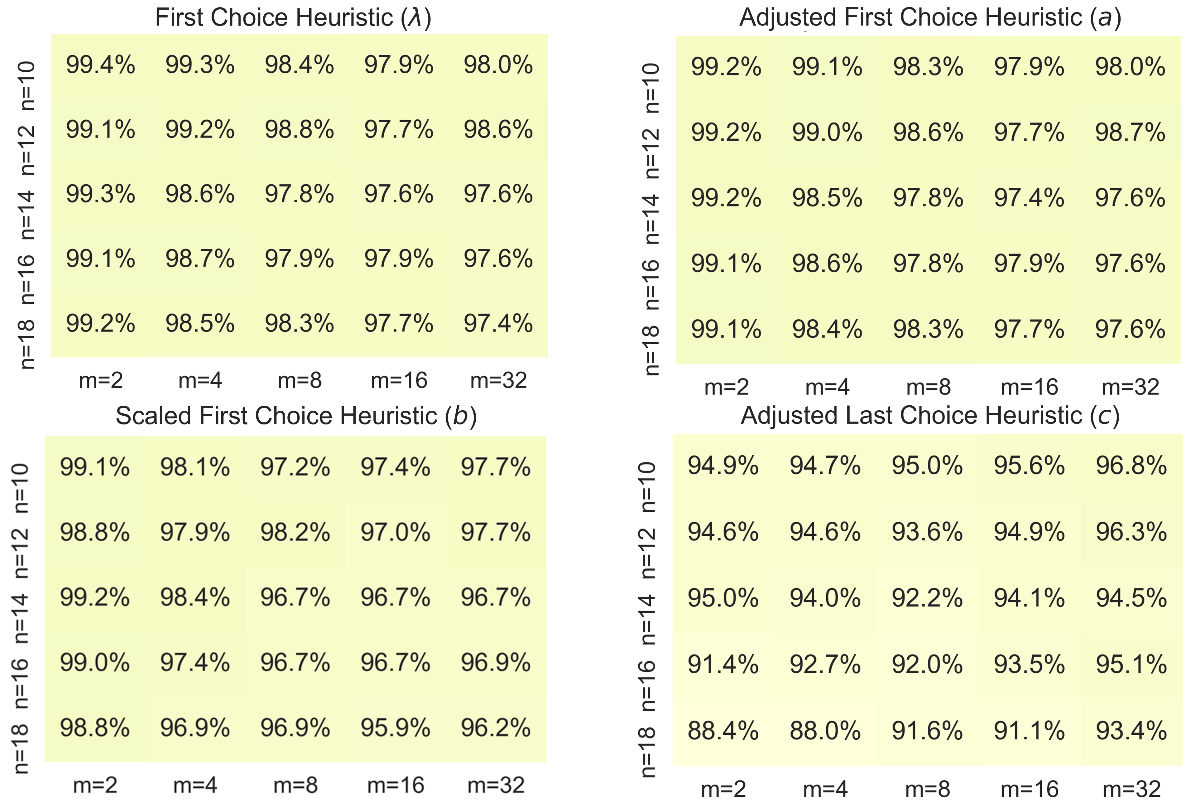
Figure 1: Performance of the four heuristics for cardinality constrained TAOP as a percentage of optimal value under the LC-MNL model. For each value of $n$ and $m$, we performed 100 experiments.

Recall that $S^{\mathcal{F}}_{x}:=\arg\max(R(S^{\mathcal{F}}_{a}),R(S^{\mathcal{F}}_{b}),R(S^{\mathcal{F}}_{c},R(S^{\mathcal{F}}_{\lambda}))$ and $\mathcal{R}^{\mathcal{F}}_{x}=R(S^{\mathcal{F}}_{x})$ define the Max-H heuristic. The performance of the Max-H heuristic is reported in the left-panel of Figure 2. Our numerical results suggest that the Max-H is consistently, but marginally, better than each of the four component heuristics. To assess the benefits of using the $S^{\mathcal{F}}_{x}$ instead of $S^{\mathcal{F}}_{\bar{v}}$, we computed the Captured Opportunity Gap (COG) defined as

$$\mbox{COG}:=\frac{\mathcal{R}^{\mathcal{F}}_{x}-R(S^{\mathcal{F}}_{\bar{v}})}{\mathcal{R}^{\mathcal{F}}-R(S^{\mathcal{F}}_{\bar{v}})}$$

and report the average COG in the right-hand panel of Figure 2 for instances in which $R(S^{\mathcal{F}}_{\bar{v}})$ is more than 5 percent below $\mathcal{R}^{\mathcal{F}}$. As can be seen, the Max-H substantially closes the gap optimality gap when $R(S^{\mathcal{F}}_{\bar{v}})$ underperforms $\mathcal{R}^{\mathcal{F}}$ by more than 5%. Thus, from a practical point of view the Max-H heuristic performs significantly better and is much easier to implement than the heuristic based on $\bar{v}$ that requires knowledge of all of the parameters of the LC-MNL model.

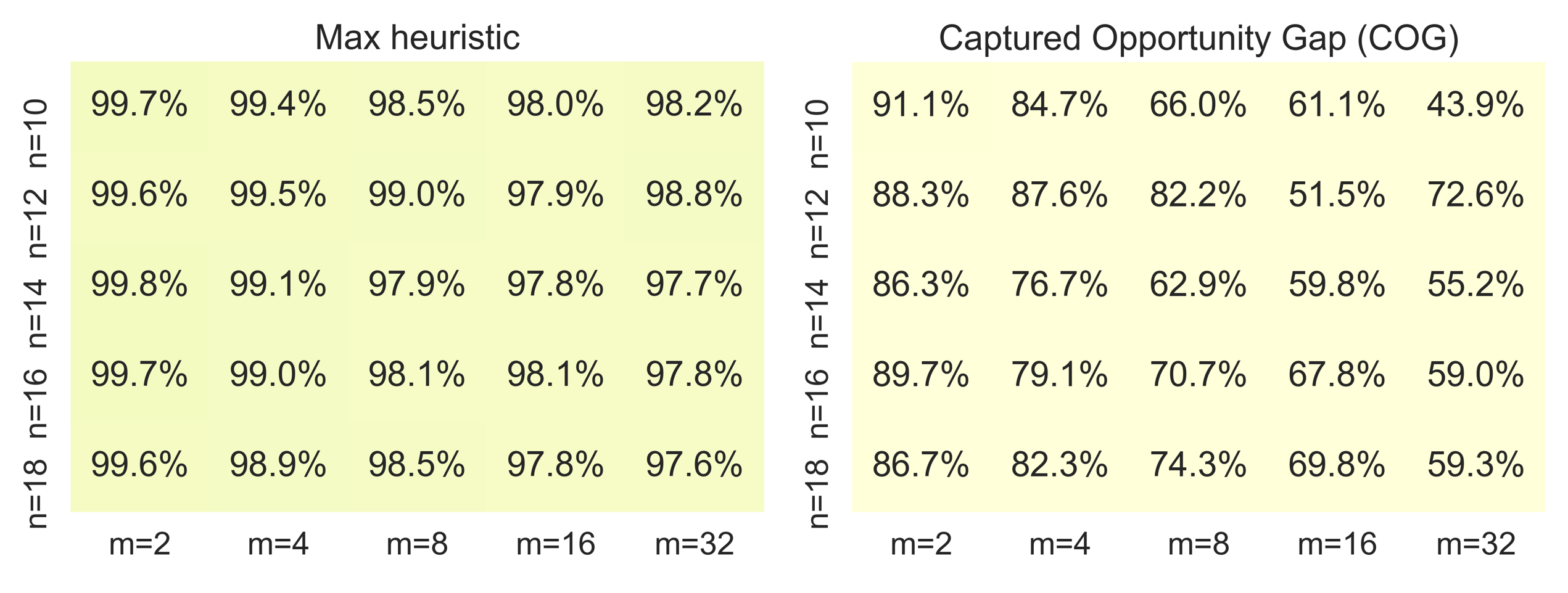
Figure 2: Left figure displays the performance of the best heuristic as a percentage of optimal value under the LC-MNL instances for cardinality constrained TAOP. Right figure shows the Captured Opportunity Gap of the Max-H.

2.1 A Refinement for Monotone Odds Ratios

In this section we briefly explore a refinements of the performance guarantees that requires some additional knowledge about the odds-ratios. Suppose that a DCM has odd-ratios satisfying

$$a^{+}_{i}:=O(i,\{i\})\leq O(i,S)\leq O(i,N)=b_{i}~{}~{}~{}\forall S\ni i~{}~{}~{}\forall i\in N.$$ (6)

A sufficient condition for (6) is that $O(i,S)$ is increasing in $S\ni i$. Examples include the generalized attraction model(GAM) (Gallego et al. 2015b), and the Random Consideration Set (RCS) model (Manzini and Mariotti 2014). The next corollary provides sharper bounds for models satisfying (6).

Corollary 2.5

If property (6) holds, then

$$\mathcal{R}^{\mathcal{F}}_{a^{+}}\leq R(S^{\mathcal{F}}_{a^{+}})\leq\mathcal{R}^{\mathcal{F}}\leq\mathcal{R}^{\mathcal{F}}_{b}$$ (7)

holds under the same conditions of Theorem 2.4.

Tighter bounds can also be obtained if:

$$a^{+}_{i}:=O(i,\{i\})\geq O(i,S)\geq O(i,N)=b_{i}~{}~{}~{}\forall S\ni i~{}~{}~{}\forall i\in N.$$ (8)

by reversing the roles of $a^{+}$ and $b$ in Corollary 2.5. As an example that fits into this situation is the standard nested MNL model with dismilarity parameters less than or equal to one. For the standard nested model (Gallego and Topaloglu 2014) show that the problem with nest-level cardinality constraints can be solved by linear programming. Our heuristic allows for a more general set of cardinality constraints.

3 The Clairvoyant Firm and the Benefits of Personalization

In this section we study the limits of personalization by modeling a clairvoyant firm that manages to sell to each arriving consumer the highest revenue product they are willing to buy. After formally introducing the clairvoyant firm, we will provide a mathematical expression for the expected revenue of the clairvoyant firm and show that it is an upper bound on the maximum revenue a firm can achieve by personalizing assortments. We will then obtain a formula to compute the expected revenue of the clairvoyant firm that works for a large class of DCMs. We will then show how to obtain an upper bound on the benefit of personalization by bounding he ratio of personalized to non-personalized policies by the ratio of the clairvoyant firm to the expected revenue of the revenue-ordered heuristic. This is followed by a numerical study on randomly generated latent-class MNL models, a dense class over the set of random utility models.

Consider a clairvoyant firm that can read the mind of each arriving consumers and sell them the highest revenue product that they are willing to buy. More precisely, let $B_{i}$ be a Bernoulli random variable that takes value one if the arriving consumer is willing to purchase product $i$ and takes value $0$ otherwise. Let $X_{i}:=r_{i}B_{i}$ denote the random revenue that the clairvoyant firm can make from selling product $i$. Since the clairvoyant firm knows the $X_{i},i\in N$ it can earn $\max_{i\in N}X_{i}$. Consequently, the clairvoyant firm makes expected revenue $\bar{\mathcal{R}}=E[\max_{i\in N}X_{i}]$.

We next compare $\bar{\mathcal{R}}$ with the optimal expected revenue, say $\mathcal{R}^{p-TAOP}$ of a p-TAOP firm that can identify the type of each arriving consumer and offer personalized assortments. More precisely, a p-TAOP firm knows that consumers follow a DCM of the form

$$\mathcal{P}(i,S)=\sum_{j\in M}\theta_{j}\mathcal{P}_{j}(i,S),$$ (9)

where $M$ represents the consumer types, or market segments, $\mathcal{P}_{j}$ represents the DCM for type $j\in M$, and $\theta_{j}>0,j\in M,\sum_{j\in M}\theta_{j}=1$ represent the weights of the different types. Let $R_{j}(S)=\sum_{i\in S}r_{i}\mathcal{P}_{j}(i,S)~{}\forall S\subset N,\forall j\in M$. A p-TAOP firm can identify the type of each arriving consumer and offer them an optimal assortment, say $S^{*}_{j}\in\arg\max_{S\subset N}R_{j}(S)$, for each $j\in M$. The p-TAOP-firm earns $\mathcal{R}^{p-TAOP}:=\sum_{j\in M}\theta_{j}\mathcal{R}_{j}(S^{*}_{j})$. The p-TAOP has been the subject of recent attention, see e.g. El Housni and Topaloglu (2023), Chen et al. (2021). Observe that if the choice model $\mathcal{P}$ is partitioned into market segments $\mathcal{P}_{j}$’s such that each $\mathcal{P}_{j}$ is a degenerate choice model, the p-TAOP firm and the clairvoyant firms coincide, so $\bar{\mathcal{R}}=\mathcal{R}^{p-TAOP}$. In general, we have that

$$\bar{\mathcal{R}}\geq\mathcal{R}^{p-TAOP}$$

since for every type $j\in M$ the clairvoyant firm knows the highest index product the consumer will buy, whereas the p-TAOP firm knows only that the consumer makes a choice according to DCM $\mathcal{P}_{j}$. Consequently, the clairvoyant firm makes at least as much revenue as the p-TAOP firm for every consumer type, and consequently a higher expected revenue overall. This clearly establishes that the expected revenue of the clairvoyant firm is an upper-bound on the expected revenue of any p-TAOP firm.

We now show that under mild conditions we can compute $\bar{\mathcal{R}}$ based on the no-purchase probabilities $\mathcal{P}(0,[i])$ of the revenue-ordered sets $[i]=\{1,\ldots,i\},i\in N$. Notice that if $\sum_{i\in N}B_{i}>0$, then $I(B):=\min\{i\in N:B_{i}=1\}$ is the index of the highest revenue product that the consumer is willing to buy. For convenience we define $I(B)=0$ when $\sum_{i\in N}B_{i}=0$. Our clairvoyant firm is able to identify $I(B)$, and to offer an arriving consumer an assortment that leads her to select alternative $I(B)$. Thus if $I(B)\in N$, the arriving consumer buys product $I(B)$, and if $I(B)=0$ she selects the outside alternative. To make the model tractable we will make the following mild assumption.

Assumption I: An arriving consumer selects $I(B)$ when offered assortment $\{I(B)\}$.

This means that if $i\in N$ is the lowest index (highest revenue) product that the consumer is willing to buy, then she would also buy when it is the only product offered. Assumption I implies $\mathcal{P}(B_{i}=1)=\mathcal{P}(i,\{i\})=\omega_{i}$, and preclude situations where an arriving consumer is willing to buy product $i$ but only if it is offered together with some other product(s). A sufficient condition for Assumption I in the context of multiple consumer types (9) is that $\mathcal{P}_{j}$ is a regular choice model for all $j\in M$. Since all RUMs are regular, Assumption I holds for all mixtures of RUMs, including the latent-class MNL.

By defining $r_{0}=0$, we have $\max_{i\in N}X_{i}=r_{I(B)}$, so $\bar{\mathcal{R}}=E[R_{I(B)}]$. We are now ready to show how to compute $\bar{\mathcal{R}}$ based on the knowledge of $\mathcal{P}(0,[i]),i\in N$.

Theorem 3.1

For any DCM that satisfies Assumption I, we have

$$\bar{\mathcal{R}}=E[R_{I(B)}]=\sum_{i\in N}r_{i}[\mathcal{P}(0,[i-1])-\mathcal{P}(0,[i])]=r_{1}-\sum_{i\in N}(r_{i}-r_{i+1})\mathcal{P}(0,[i]).$$

All of the results in the remainder of the paper are limited, without further mentioning, to choice models that satisfy Assumption I. We next apply Theorem 3.1 to DCMs that have independent $B_{i}$s, $i\in N$. In this case $\mathcal{P}(0,[i])=\Pi_{j\leq i}\mathcal{P}(B_{j}=0)=\Pi_{j\leq i}(1-\omega_{j})$, so

$$\bar{\mathcal{R}}=\sum_{i\in N}r_{i}[\Pi_{j\leq i-1}(1-\omega_{j})-\Pi_{j\leq i}(1-\omega_{j})]=\sum_{i\in N}r_{i}\Pi_{j\leq i}(1-\omega_{j})\omega_{i}.$$ (10)

We next apply Theorem 3.1 to the MNL model. For this model, it is easy to see that $\mathcal{P}(0,[i-1])-\mathcal{P}(0,[i])=\mathcal{M}_{v}(0,[i-1])\mathcal{M}_{v}(i,[i])$, so Proposition 1 results in

$$\bar{\mathcal{R}}_{v}=\sum_{i\in N}r_{i}\mathcal{M}_{v}(0,[i-1])\mathcal{M}_{v}(i,[i]).$$ (11)

For the latent class MNL model we have,

$$\bar{\mathcal{R}}=\sum_{j\in M}\theta_{j}\bar{\mathcal{R}}_{j}$$ (12)

where $\theta_{j}$ is the proportion of type $j$ consumers, and $\bar{\mathcal{R}}_{j}$ is the expected revenue of a clairvoyant firm when the type $j$ consumer follows an MNL with attraction vector $v_{j}$.

When the data $\mathcal{P}(0,[i]),i\in N$ needed to compute $\bar{\mathcal{R}}$ are not available, we can use the following bounds on $\bar{\mathcal{R}}$ that are based on $\hat{\mathcal{R}}_{\omega}=\min_{\tau}[\tau+\sum_{i\in N}(r_{i}-\tau)^{+}\omega_{i}]$ and $\mathcal{R}^{*}_{\omega}$, where $\omega$ is the vector of last-choice probabilities.

Theorem 3.2

$$\bar{\mathcal{R}}\leq\hat{\mathcal{R}}_{\omega}\leq 2\mathcal{R}^{*}_{\omega}.$$

The last bound, although numerically superfluous, will be useful later in establishing prophet inequalities.

We now have enough theory to assess, in the limit, the benefit of personalization. This requires that we can compute $\bar{\mathcal{R}}$ via the formula presented in Theorem 3.1 or the upper bound $\hat{\mathcal{R}}_{\omega}$ of Theorem 3.2. Clearly

$$\mathcal{R}^{0}\leq\mathcal{R}^{*}\leq\mathcal{R}^{p-TAOP}\leq\bar{\mathcal{R}}\leq\hat{\mathcal{R}}_{\omega}.$$

Consequently, we have

$$\frac{\mathcal{R}^{p-TAOP}}{\mathcal{R}^{*}}\leq\frac{\bar{\mathcal{R}}}{\mathcal{R}^{*}}\leq\frac{\bar{\mathcal{R}}}{\mathcal{R}^{o}}\leq\frac{\hat{\mathcal{R}}_{\omega}}{\mathcal{R}^{o}}$$ (13)

which bounds the benefits of personalization when we can compute $\bar{\mathcal{R}}$ (or $\hat{\mathcal{R}}_{\omega})$ and either $\mathcal{R}^{*}$ or $\mathcal{R}^{o}$. In many cases, we would have enough information, namely the $\mathcal{P}(0,[i]),i\in N$ to compute $\bar{\mathcal{R}}$, but computing $\mathcal{R}^{*}$ may be an NP-hard so we can use $\mathcal{R}^{o}$ as suggested in (13).

We next present results of computational experiments under the LC-MNL model to study the relative performance of traditional assortment optimization, personalized assortment optimization and the clairvoyant firm. We present these results as percentages of the revenue obtained for a TAOP-firm that employs the revenue-ordered assortment heuristic.

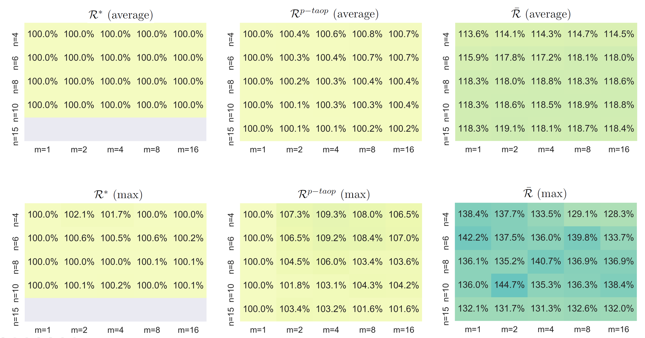
Figure 5: Scenario 3: $\beta=2$. Performance of TAOP, personalized TAOP and a clairvoyant as a percentage of revenue-ordered profits under the LC-MNL model. For each value of $n$ and $m$, we performed 300 experiments.

The instances for the numerical study follow a well accepted procedure to generate random instances first proposed by Rusmevichientong et al. (2014). The utility of $i\in N$ to type $j\in M$ is modeled as $U_{ij}=u_{ij}+\epsilon_{ij}$ where $u_{ij}$ is the deterministic part of the utility and $\epsilon_{ij},i\in N_{+}$ are standard Gumbel random variables with mean zero and variance $\pi^{2}/6$, corresponding to scale parameter 1 and location parameter $-\gamma$ where $\gamma$ is the Euler’s constant. By setting $u_{ij}=a_{ij}/\beta$ for a parameter $\beta>0$ we can control the variance of the utilities. Indeed, by multiplying all the utilities by $\beta$, the variance of each Gumbel changes to $\pi^{2}\beta^{2}/6$. Notice that the exponentiated utilities are given by $v_{i}=\exp(a_{ij}/\beta)$. In our experiments, we fixed the lowest revenue to $1$ and the highest revenue to $10$, and select the revenues of the rest of the products uniformly between $1$ and $10$. For each combination of $(m,n)$ we generated 300 random instances. For each instance, the $a_{ij},i\in N_{+}$ are chosen randomly following Rusmevichientong et al. (2014) and present results for four different values of $\beta$: 0.02 (fig. 3); 0.2 (fig. 4); 2 (fig. 5), and 20 (fig. 6). For each of those four scenarios, we calculate the optimal revenue obtained under TAOP; personalized TAOP (p-TAOP); and the clairvoyant firm ($\bar{\mathcal{R}}$) as a percentage of the revenue obtained using revenue-ordered assortments heuristic under traditional assortment optimization. Each figure reports the average and maximum percentage across the 300 instances.

Our computational experiments suggest that the revenue-ordered heuristic performs relatively well even against a clairvoyant firm. Indeed, from our experiments we see that the expected revenues of the clairvoyant firm are, on average, between 0.5% to 19% higher than the expected revenues under the revenue-ordered heuristic. On the other hand, the personalized heuristic is on average 0% to 10.8% higher than the expected revenue of the revenue-ordered heuristic.

A much clearer picture emerges when we study the numerical results for different values of $\beta$ which is a proxy for the variance of the utilities $U_{ij},i\in N,j\in M$. For $\beta=0.02$ (fig 3) there can be a significant gap between $\mathcal{R}^{p-TAOP}$ and $\mathcal{R}^{*}$, but a relatively small gap between the p-TAOP and the clairvoyant firm. Exploring instances where the p-TAOP firm makes significant gains over the TAOP firm, we see that these instances have both low utility variance and relatively high heterogeneity in the mean utilities. This makes sense because with heterogeneity and low variance a p-TAOP firm can guess with high probability what product(s) the consumer is likely to buy. This also suggests that in this instances the gap between the p-TAOP and the clairvoyant firm should be small! This is indeed confirmed by instance $(m,n)=(16,4)$ where on average the p-TAOP makes 10.8% more than the revenue-ordered heuristic while the clarivoyant firm makes 11.4% more than the revenue-ordered heuristic.

We can make these insights more formal by looking at what happens as $\beta\downarrow 0$. Suppose that the random utilities $U_{ij}=u_{ij}+\epsilon_{ij},i\in N_{+},j\in M$ are such that for every $j$ there the $u_{ij}$s are well spread, and the variance of the $\epsilon_{ij},i\in N$ are small for every $j\in M$. Then, for each customer segment the model converges to a maximum utility model. Consequently, the p-TAOP firm can personalize assortments based on the purchase probabilities $\mathcal{P}_{j}(i,\{i\})=\omega_{ij}$ which in the limit are either $0$ or $1$. Thus, as $\beta\downarrow 0$, the ability of the p-TAOP firm approaches the ability of the clairvoyant firm. This justifies why for small $\beta$ we see a small gap between the expected revenue of a p-TAOP firm and the clairvoyant firm. In this case, the p-TAOP and the clairvoyant firm have a significant advantage relative to the TAOP firm as long as there is heterogeneity among the different consumer types, and also heterogeneity in the $r_{i},i\in N$.

On the other hand, when $\beta=20$ (Fig 6) the optimal revenue under the TAOP and the p-TAOP are almost indistinguishable from each other and from the expected revenue of the revenue-ordered heuristic. Indeed, the p-TAOP makes at most 0.8% on average more than the revenue-oredered heuristic over all the $(m,n)$ combinations. Notice also that there is a significant gap between the p-TAOP and the clairvoyant firm, but the ratio is never larger than 1.5.

We can also make these insights more formal. First, if the variances are large then the exponetiated utilities $v_{ij}=\exp(u_{ij}/\beta)\simeq 1$. So the DCM for each $j\in M$ becomes close to an MNL with attraction vector $v=e$. In this case, the LC-MNL itself resembles an MNL with $v=e$. It is clear that in the limit there is no advantage of personalization and therefore $\mathcal{R}^{p-TAO}=\mathcal{R}^{*}=\mathcal{R}^{0}$. On the other hand, the clairvoant firm has a decisive advantage! In the next theorem we show that this allows the clairvoant firm to earn up to 1.5 more than a TAOP firm. This result supports are numerical finding that the clairvoyant firm never makes more than 1.5 more than the TAOP firm.

To present the theorem we need some notation. Let $\mathcal{R}^{*}(\beta)$ and $\bar{\mathcal{R}}(\beta)$ be the optimal expected revenues, respectively for the TAOP and the clairvoyant firm as a function of $\beta$ for the LC-MNL. Also, let $e$ be the vector of ones, and $\mathcal{R}^{*}_{e}$ the optimal expected revenue of an MNL with $v=e$.

Theorem 3.3

$$\mathcal{R}^{*}_{e}=\lim_{\beta\rightarrow\infty}\mathcal{R}^{*}(\beta)\leq\lim_{\beta\rightarrow\infty}\bar{\mathcal{R}}(\beta)=\bar{\mathcal{R}}_{e}\leq 1.5\mathcal{R}^{*}_{e}.$$

This result is also valid if the products for each consumer type have a different $\beta_{j},j\in M$ and $\beta_{j}\rightarrow\infty$ for all $j\in M$. In practice, it does not take a very large $\beta$ for $\mathcal{R}^{*}(\beta)$ and $\bar{\mathcal{R}}(\beta)$ to be well approximated by $\mathcal{R}^{*}_{e}$ and $\bar{\mathcal{R}}_{e}$.

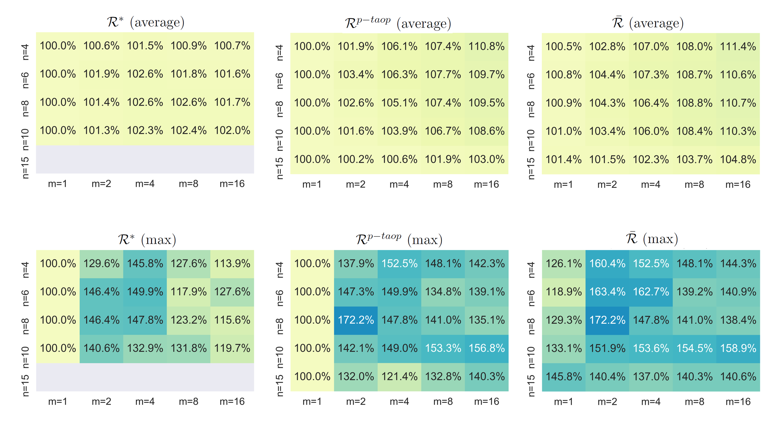
Figure 3: Scenario 1: $\beta=0.02$. Performance of TAOP, personalized TAOP and a clairvoyant as a percentage of revenue-ordered profits under the LC-MNL model. For each value of $n$ and $m$, we performed 300 experiments.

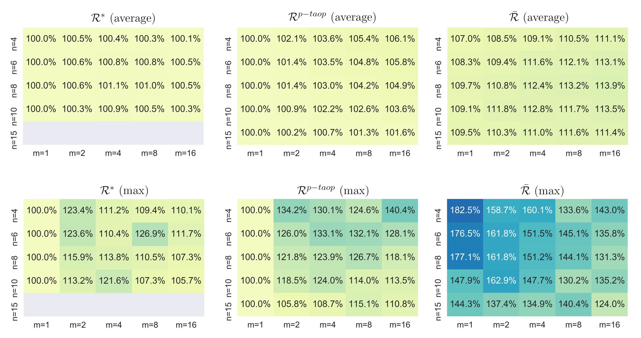
Figure 4: Scenario 2: $\beta=0.2.$ Performance of TAOP, personalized TAOP and a clairvoyant as a percentage of revenue-ordered profits under the LC-MNL model. For each value of $n$ and $m$, we performed 300 experiments.

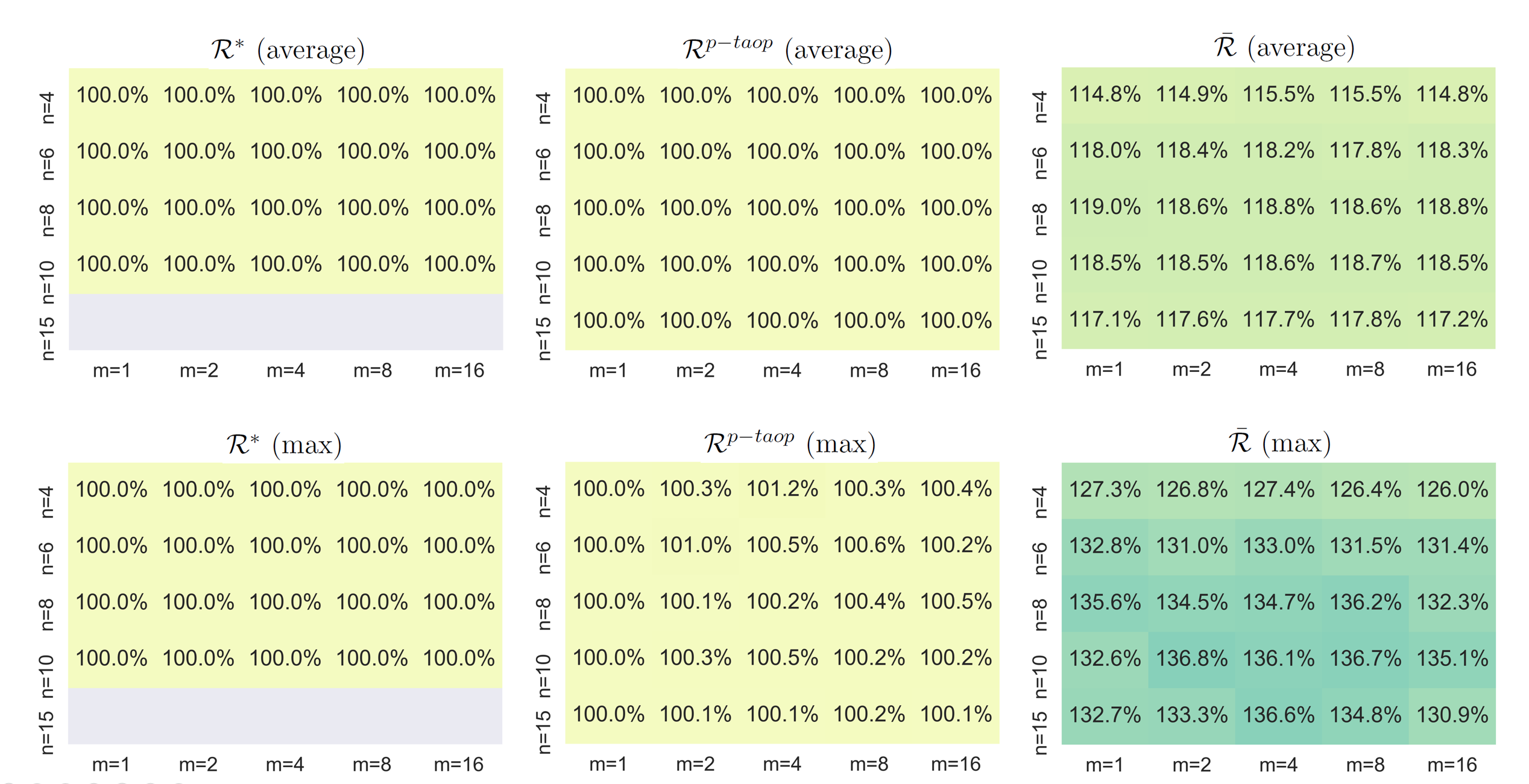
Figure 6: Scenario 4: $\beta=20$. Performance of TAOP, personalized TAOP and a clairvoyant as a percentage of revenue-ordered profits under the LC-MNL model. For each value of $n$ and $m$, we performed 300 experiments.

3.1 Benefits of Personalization: Extreme Cases

While the bound (13) is practically useful to assess the benefits of personalziation for a particular instance or for a set of randomly generated instances, it does not provide us with a good idea how large the right-hand side of (13) can be, or whether there are conditions under which a firm can earn as much revenue in expectation as a clairvoyant firm, and therefore as much revenue as any attempt to personalize assortments. It is possible to construct examples where a clairvoyant firm can make arbitrarily more than a TAOP firm when we allow non-regular DCMs, so for the rest of this section we concentrate on regular discrete choice models. In this section we show that within the class of regular models it is possible to construct examples where the clairvoyant firm makes $n$ times as much as the TAOP firm and examples where the TAOP firm makes as much as the clairvoyant firm. This statement is true even for the class of Markov Chain models.

Theorem 3.4

For all regular DCMs

$$\mathcal{R}^{p-TAOP}\leq\bar{\mathcal{R}}\leq n\mathcal{R}^{o}\leq n\mathcal{R}^{*}$$ (14)

Moreover, we can construct a sequence of instances where $\bar{\mathcal{R}}=\mathcal{R}^{p-TAOP}\geq n\mathcal{R}^{*}-\epsilon$ for all $\epsilon>0$. These results remain true even within the class of Markov chain choice models.

Theorem 3.4 tells us that for all regular DCMs the inequality $\bar{\mathcal{R}}\leq n\mathcal{R}^{*}$, and that there are instances of regular choice models for which $\bar{\mathcal{R}}\geq\mathcal{R}^{p-TAOP}\geq n\mathcal{R}^{*}-\epsilon$ for any $\epsilon>0$ even if we restrict DCMs to the class of Markov chain choice models.

It is also interesting to contrast the factor $n$ gap between $\bar{\mathcal{R}}$ and $\mathcal{R}^{*}$ within the class of Markov chain models with a recent result in Ma (2022). That paper studies how much a firm can increase its expected revenue relative to TAOP by allowing certain products to be only available through lotteries (this is a lower bound of the clairvoyant profit). The author showed that unless $P=NP$, there is no constant factor for the ratio relative to the TAOP for general RUMs, and on the other hand the firm cannot increase their revenue using lotteries for Markov chain choice model.

We next show that for the independent demand model the TAOP firm can make as much as the clairvoyant firm. The independent demand model is defined by $\mathcal{P}(i,S)=\lambda_{i}$ for all $i\in S$, and $\mathcal{P}(0,S)=1-\sum_{i\in S}\lambda_{i}$. The independent demand model gets its name from the fact that $\mathcal{P}(i,S)$ is independent of $S\ni i$. This model, however, does not have independent $B_{i},i\in N$. In fact if $B_{i}=1$ for some $i\in S$, then $B_{k}=0$ for all $k\in S,k\neq i$. For the independent demand model we have $R(S)=\sum_{i\in S}r_{i}\lambda_{i}$, and it is clear that $\mathcal{R}^{*}=R(N)=\sum_{i\in N}r_{i}\lambda_{i}$. From Theorem 3.1 we see that $\mathcal{P}(I(B)=i)=\mathcal{P}(0,[i-1])-\mathcal{P}(0,[i])=\lambda_{i},i\in N$ implying that $\bar{\mathcal{R}}=\sum_{i\in N}r_{i}\lambda_{i}=\mathcal{R}^{*}$. We summarize this finding in the next proposition.

Proposition 3.5

For the independent demand model, $\bar{\mathcal{R}}=\mathcal{R}^{*}$, so the clairvoyant firm cannot make more than the TAOP firm.

Intuitively, a clairvoyant firm that knows that an arriving consumer is willing to buy product $i$ would offer assortment $\{i\}$. However, such a consumer is only interested in product $i$ and would also buy product $i$ if the offered assortment is $N$, so the two firms earn the same revenue for each arriving consumer, and hence earn the same expected revenue.

Interestingly, there is another way that a firm can earn as much as a clairvoyant firm by offering products sequentially in decreasing order of revenues. To achieve revenues as high as the clairvoyant firm, consumers need to be persistent and follow a satisfying policy. A consumer is said to follow a satisfying policy, see (Gao et al. 2021), if she makes a purchase as soon as she sees a product that is preferred to the outside alternative. A consumer is said to be persistent if she continues examining products until she either finds a satisfying product or exhausts the product list. The next result shows that if consumers follow a persistent-satisfying policy then a non-clairvoyant firm can earn $\bar{\mathcal{R}}$ without even knowing the specific form of the DCM or its underlying parameters, and makes clear the potential gains of sequential offerings over traditional assortments.

Proposition 3.6

A non-clairvoyant firm can earn $\bar{\mathcal{R}}$ by offering products sequentially in the order $1,2,\ldots,n$ (from high-to-low revenues) to consumers who follow a persistent-satisfying policy.

4 Prophet Inequalities for Assortment Optimization

We next address a connection between the assortment optimization problem and the classical prophet problem (see, e.g. Lucier (2017) for a recent review of this literature). This connection will allow us to show that if the $B_{i},i\in N$ are independent, then the bound in (13) is at most 2. In the prophet problem, the rewards $X_{i},i\in N$ are assumed to be independent, non-negative, random variables. The decision maker sees the $X_{i}$’s, one at a time, in a given order, say $\sigma(i)~{}i\in N$, where $\sigma$ is a permutation of $N$. Upon observing $X_{\sigma(i)}$, the decision maker decides whether to take the reward $X_{\sigma(i)}$ or move on to the next reward $\sigma(i+1)$ without the recourse of going back to previously passed rewards. The challenge is to compare the optimal expected reward of the decision maker to the expected reward $\bar{\mathcal{R}}=E[\max_{i\in N}X_{i}]$ of a prophet that knows the realized values of the $X_{i},i\in N$. Krengel and Sucheston (1977) show that there exists a heuristic for the decision maker that is robust in the sense that it always yields at least half of $\bar{\mathcal{R}}$ in expectation. The heuristic is in the form of a threshold policy, where the decision maker selects the first product, if any, with reward exceeding the threshold.

Notice that both clairvoyant firm and the prophet earn $E[\max_{i\in N}X_{i}]$. One difference between the two problems is that for the clairvoyant firm the $X_{i}$s are in general dependent random variables while they are independent for the prophet problem. In addition, in the clairvoyant problem the $X_{i}$s can only take values in $\{0,r_{i}\}$, whereas in the prophet problem the $X_{i}$s do not have this restriction. There is also some parallels between the decision makers. In our model, consumers observe the entire assortment before selecting an alternative. In contrast, in the prophet problem the decision maker observes the products in a certain order and must make a selection without recourse. Given the differences and similarities, the reader may wonder whether a prophet type inequality holds for the clairvoyant firm. The answer is yes as shown in the next proposition.

Proposition 4.1

The prophet inequality applies to the assortment optimization problem with independent $B_{i},i\in N$, implying that

$$\mathcal{R}^{*}\leq\bar{\mathcal{R}}\leq 2\mathcal{R}^{*}.$$ (15)

Moreover, the bound is tight, and in addition the following inequality holds

$$\mathcal{R}^{o}\leq\bar{\mathcal{R}}\leq 2\mathcal{R}^{o}.$$

The main idea is that for the threshold policy $\tau$ in the prophet problem, there is a corresponding revenue-ordered assortment $S(\tau)=\{i\in N:r_{i}>\tau\}$. The argument then reduces to showing that $R(S(\tau))$ is at least as large as the expected reward of the threshold policy under the worst possible ordering. Notice that the worst possible ordering for the decision maker is the one that ranks products from the lowest to the highest $r_{i},i\in N$. If product $i$ with $X_{i}>\tau$ is selected by the decision maker then $B_{i}=1$ and $r_{i}>\tau$, implying that $i\in S(\tau)$. Moreover, $B_{j}=0$ for all $j\in S(\tau)$ with $r_{j}<r_{i}$, so a consumer offered $S(\tau)$ would either buy $i\in S(\tau)$ or another product in $S(\tau)$ with $r_{j}>r_{i}$. This implies that the firm offering assortment $S(\tau)$ earns at least as much as the decision maker using threshold $\tau$ who sees the products sequentially in increasing order of revenues. Since the prophet inequality asserts that even under the worst ordering the decision maker earns at least $0.5\bar{\mathcal{R}}$ it follows that $0.5\bar{\mathcal{R}}\leq R(S(\tau))\leq\mathcal{R}^{o}\leq\mathcal{R}^{*}$.

Proposition 4.1 applies directly to RUMs where the value gaps $U_{i}-U_{0},i\in N$ are independent random variables. This holds, for example if the $U_{i},i\in N$ are independent and $U_{0}$ is deterministic. The assortment optimization problem for the special case where $U_{i},i\in N$ are independent Gumbel random variables and $U_{0}$ is deterministic is NP-hard as shown by (Wang 2021). By Proposition 4.1 the TAOP firm earns at least half as much as the clairvoyant firm even if it just uses the revenue-ordered heuristic.

The random variables $B_{i},i\in N$ are also independent, by definition, in the random consideration set (RCS) model (Manzini and Mariotti 2014), where the last-choice probabilities $\mathcal{P}(B_{i}=1)$ are known as attention-probabilities. In their model their is a preference ordering, so all consumers purchase the first product with $B_{i}=1$ in the given order. The assortment optimization problem for the RCS model was first considered by Gallego and Li (2017), who proved that the revenue-ordered heuristic has a 1/2 performance guarantee. By Proposition 4.1 the revenue-ordered heuristic yields at least half of the expected profits of the clairvoyant firm strengthening their result. Notice that for independent $B_{i},i\in N$, the formula for $\bar{\mathcal{R}}=\sum_{i\in N}\Pi_{j<i}(1-\omega_{j})\omega_{i}r_{i}$ $B_{i},i\in N$, coincides with the expected revenue of a RCS model where the preference order is $\{1,\ldots,n\}$. It is not difficult to see that the lowest possible revenue for the RCS model stems from the preference ordering $\{n,n-1,\ldots,1\}$. By the prophet inequality, the ratio of the expected revenues corresponding to the best and worst orderings is at most 2, a fact that can be challenging to establish without the aid of Proposition 4.1.

4.1 Prophet Inequalities for Models with Dependent Value Gaps

Unfortunately the prophet inequality does not easily extend to models where the $X_{i}$s are dependent, and models where the $X_{i}$s are positively correlated are particularly difficult to deal with. On the other hand, for many DCMs the $B_{i}$’s are positively correlated. As an example, for RUMs the $B_{i}$s are indicator functions of $U_{i}-U_{0}\geq 0$, which induces negative correlation when $U_{0}$ is random. Correlation among the $B_{i},i\in N$ precludes us from using Theorem 3.4. In this section we make progress in the quest of finding DCMs with dependent $B_{i},i\in N$ for which the prophet inequality (15) still holds, so the clairvoyant firm cannot make more than twice the expected revenue of a TAOP firm.

We are now ready to provide our first sufficient condition for the prophet inequality to hold without the independence of the $B_{i},i\in N$.

Theorem 4.2

A sufficient condition for the prophet inequality (15) to hold is

$$\mathcal{R}^{*}_{\omega}\leq\mathcal{R}^{o}.$$ (16)

Condition (16) can be checked numerically in $O(n)$ time by computing $\mathcal{R}^{*}_{\omega}$ and $\mathcal{R}^{o}$. Building upon Theorem 4.2, we prove the prophet inequality for the MNL model.

Theorem 4.3

The prophet inequality holds in the assortment optimization problem under the MNL model. Thus,

$$\bar{\mathcal{R}}\leq 2\mathcal{R}^{*}.$$ (17)

Moreover, the bound is tight.

By Theorem 4.3, the clairvoyant firm cannot make more than twice than the TAOP firm when the underlying DCM is an MNL. The reader may wonder whether a prophet inequality will extend to personalized assortments when each type is governed by an MNL. This brings us back to model (9) for the special case where type $j$ consumers follow an MNL with attraction vector $v_{j}=(v_{ij})_{i\in N}$. If the firm can observe the type of each arriving consumer and offer them a personalized assortment the p-TAOP firm earns expected revenue

$$\mathcal{R}^{p-taop}=\sum_{j\in M}\theta_{j}\mathcal{R}^{*}_{j},$$

where $\mathcal{R}^{*}_{j}$ is the optimal expected revenue for type $j$ consumers. On the other hand, the clairvoyant firm earns $\bar{\mathcal{R}}:=\sum_{j\in M}\theta_{j}\bar{\mathcal{R}}_{j}$, where $\bar{\mathcal{R}}_{j}:=\sum_{i=1}^{n}r_{i}\mathcal{M}_{j}(0,[i-1])\mathcal{M}_{j}(i,[i])$ is the expected profit of the clairvoyant firm for type $j$ consumers. The next corollary shows that the prophet inequality also holds in this case.

Corollary 4.4

If each market segment is governed by an MNL model,

$$\mathcal{R}^{p-taop}\leq\bar{\mathcal{R}}\leq 2\mathcal{R}^{p-taop}.$$

Corollary 4.4 asserts that under a LC-MNL model, a clairvoyant firm cannot make more than two times the optimal expected revenue of a p-TAOP firm that can customize an assortment to each MNL segment.

The reader may wonder whether the prophet inequality also holds for other models such as the generalized attraction model (GAM) or some versions of the nested logit (NL) model. Unfortunately condition (16) does not hold for these models, so other methods are needed. We next present a second sufficient condition for a class of models that includes the GAM and the non-standard NL model where each of the dissimilarity parameters is at least one.

Proposition 4.5

Let $\mathcal{P}$ be a regular choice model with $\lambda_{0}>0$ and $O(i,S)\geq O(i,\{i\})=a^{+}_{i}$ for all $S\ni i~{}~{}\forall~{}i\in N$. Then the prophet inequality (15) holds. In particular, the prophet inequality holds for the GAM, and for the non-standard NL model.

The intuition is that if $O(i,S)\geq a^{+}_{i}$, then $a^{+}_{i}=\omega_{i}/(1-\omega_{i})\geq\omega_{i}$, so by Lemma 2.3, $\mathcal{R}^{*}_{\omega}\leq\mathcal{R}^{*}_{a^{+}}\leq R(S^{*}_{a^{+}})\leq\mathcal{R}^{o}$ showing that the sufficient condition (16) holds. It is easy to verify that $O(i,S)\geq a^{+}_{i},~{}\forall i\in N$ holds for the GAM and for the non-standard nested logit model.

In some cases we can obtain prophet-type inequalities that guarantee that the clairvoyant firm can earn at most $2/\phi$ times what can be earned by a regular firm, where $\phi$ is an instance dependent parameter.

Theorem 4.6

For any $\phi>0$, let $\mathcal{R}^{*}_{\phi\omega}$ be the expected revenue of an auxiliary MNL with parameters $\phi\omega$, and let $S^{*}_{\phi\omega}=\{i\in N:r_{i}>\mathcal{R}^{*}_{\phi\omega}\}$. If

$$\mathcal{O}(i,S^{*}_{\phi\omega})\geq\phi\omega_{i}~{}~{}~{}~{}\forall~{}i\in S^{*}_{\phi\omega}$$ (18)

holds for $\phi=1$ then the prophet inequality (15) holds. Else, let $\phi^{*}<1$ be the largest $\phi$ for which (18) holds. Then

$$\frac{\bar{\mathcal{R}}}{\mathcal{R}^{*}}\leq\frac{2}{\phi^{*}}.$$

Moreover, the revenue-ordered heuristic $\mathcal{R}^{o}$ achieves at least half of the revenue of the clairvoyant firm if (18) holds for $\phi=1$, and at least $\phi^{*}/2$ otherwise.

We remark (18) is much weaker than the condition of Proposition (4.5) as we only require the odds ratios $O(i,S^{*}_{\phi\omega})$ for $i\in S^{*}_{\phi\omega}$ to be bounded below. Verifying condition (18) for $\phi=1$ requires $O(n)$ work.

The following corollary provides an easy to compute, but somewhat crude, performance guarantee for the revenue-ordered heuristic relative to the clairvoyant firm. To obtain this bound, we find the largest $\phi$ such that $a_{i}\geq\phi\omega_{i}$ holds for all $i\in N$. This yields

$$\phi_{\min}=\min_{i\in N}\frac{a_{i}}{\omega_{i}}=\min_{i\in N}\frac{\lambda_{i}}{\omega_{i}(1-\omega_{i})}.$$

As a consequence we have the following corollary.

Corollary 4.7

For all regular DCMs with $\lambda_{0}>0$,

$$\frac{\bar{\mathcal{R}}}{\mathcal{R}^{*}}\leq\frac{\bar{\mathcal{R}}}{\mathcal{R}^{o}}\leq\frac{2}{\phi_{\min}}=2\max_{i\in N}\frac{\omega_{i}(1-\omega_{i})}{\lambda_{i}}.$$

We remark that $\phi_{\min}$ can be computed in $O(n\log n)$ time as it involves finding the smallest among $n$ numbers $a_{i}/\omega_{i}$. The advantage of Corollary 2 is that it can give us a very quick measure of the maximum benefits of personalized assortments based only on information of the first and last-choice probabilities, relative to both the TAOP-firm and the revenue-ordered heuristic.

We next examine the LC-MNL model. Since any RUM can be approximated arbitrarily close by a latent class MNL (LC-MNL) model (Chierichetti et al. 2018), and Theorem 3.4 shows that the ratio can be as large as $n$, there is no hope for a general prophet inequality for the non-personalized LC-MNL. What we seek instead, is to find conditions under which the prophet inequality holds.

For non-personalized assortments the firm attempts to maximize

$$R(S):=\sum_{j\in M}\theta_{j}R_{j}(S)$$

over $S\subset N$. This is well known to be NP-hard (add references here). Abusing notation, we can write the last-choice probabilities for the LC-MNL as:

$$\omega_{i}=\mathcal{P}(i,\{i\})=\sum_{j\in M}\theta_{j}\mathcal{M}_{j}(i,\{i\})=\sum_{j\in M}\theta_{j}\omega_{ij},i\in N$$

where $\omega_{ij}=v_{ij}/(1+v_{ij})$. We can then define the vector $\omega$ with components $\omega_{i},i\in N$, and for this vector we compute $\mathcal{R}^{*}_{\omega}$ and $S^{*}_{\omega}$. Then condition (18) for $\phi=1$ is equivalent to

$$\sum_{j\in M}\theta_{j}(v_{ij}-\omega_{i})\mathcal{M}_{j}(0,S^{*}_{\omega})\geq 0~{}~{}~{}\forall i\in S^{*}_{\omega}.$$ (19)

We remark that condition (19) can be checked very efficiently for $\omega$ as it merely requires computing $\omega$, $\mathcal{R}^{*}_{\omega}$ and $S^{*}_{\omega}$ in order to verify whether or not (19) holds.

Corollary 4.8

Consider the LC-MNL model. If condition (19) holds , then the prophet inequality (15) holds for the LC-MNL, and if it fails then there is a largest $\phi<1$, say $\phi^{*}$, such that

$$\sum_{j\in M}\theta_{j}(v_{ij}-\phi\omega_{i})\mathcal{M}_{v_{j}}(0,S)\geq 0~{}~{}~{}\forall i\in S^{*}_{\phi\omega},$$

resulting in

$$\frac{\bar{\mathcal{R}}}{\mathcal{R}^{o}}\leq\frac{2}{\phi^{*}}.$$

To explain why the numerical examples of Section 3 show an extraordinarily good performance relative to the worst case bound obtained in Theorem 3.4, and even relative to the prophet inequality (15), we start by noticing that the condition (19) holds in the vast majority of the generated instances (in all instances in some regimes) giving a theoretical justification of why we never saw in our computational study any instance where the ratio is 2 or higher.

5 Discussion

We proposed a set of auxiliary MNL models that allowed us to provide lower and upper bounds on the optimal expected revenue for all regular DCMs for the TAOP with with TUM constraints, opening the door to the development of simple heuristics that require only knowledge of the first and last-choice probabilities. We then studied the limits of assortment personalization by considering the extreme case in which a firm is clairvoyant. Based on an auxiliary MNL model, we have shown that a clairvoyant firm can make no more than twice as much as the best revenue-ordered assortment for the MNL, for personalized assortments based on the LC-MNL, and for the GAM. At the same time, we provide sufficient conditions that can be used to test whether or not the prophet inequality holds for particular DCMs. Sharper inequalities also emerge for the LC-MNL model when the coefficient of variation of all the products is large, explaining why the revenue-ordered assortment perform so well in practice in such situations. Our computational results for the LC-MNL model support our theoretical results and show that the best revenue-ordered assortments does remarkably well even against a clairvoyant firm. For instance, those results show that the increase in profits when switching from a TAOP-firm that uses revenue-ordered assortments to a clairvoyant firm was never more than 20 percent on average ($n\leq 15,m\leq 16$). We now discuss some extensions to our model.

5.1 Personalized Assortments and TUM constraints

We have explored separately the issues of personalization and assortment optimization under TUM constraints. Conceivably a firm may want to both personalize assortments and offer each market type an assortment that satisfies TUM constraints. If the p-TAOP is given by a LC-MNL then we can solve the $\mathcal{F}$-TAOP problem exactlt for each market segment. Otherwise, we can use the heuristic of Section 2 for each of the market segments obtaining bounds and heuristics for each segment. More precisely, for each market segment $j\in M$, we can use the Max-H heuristic to find a feasible assortment, say $S^{\mathcal{F}}_{x}(j)$, and its expected revenue $R(S^{\mathcal{F}}_{x}(j),j)$. Then, we can compare the expected revenue of the personalized heuristic $\sum_{j\in M}\theta_{j}R(S^{\mathcal{F}}_{x}(j),j)$ with the expected revenue, say $R(S^{\mathcal{F}}_{x})$, for the non-personalized solution. In the downwardly feasible case, we can also obtain an upper bound, say $\sum_{j\in M}\theta_{j}R(S^{\mathcal{F}}_{c}(j),j)$ on the benefits of personalization under TUM constraints. Further work is needed to establish more refined results such as precise conditions for the prophet inequalities to hold for constrained versions of the problem.

5.2 Clairvoyant pricing

Consider now a clairvoyant firm that observes the gross utilities $U_{i},i\in N_{+}$ of each incoming consumer. How should such a clairvoyant firm set prices to maximize expected revenues? For $n=1$, it is optimal to set $p_{1}$ as the largest non-negative price such that $U_{1}-p_{1}\geq U_{0}$. Then a sale occurs at $p_{1}=U_{1}-U_{0}$ if $U_{1}\geq U_{0}$. On the other hand, if $U_{1}<U_{0}$ the firm sets the price at $p_{1}=0$ and the consumer walks away without buying. Consequently, for the case of a single product the firm prices at $p_{1}=(U_{1}-U_{0})^{+}$ and earns $E[(U_{1}-U_{0})^{+}]$ in expectation. Notice here that a product may be sold at a positive price even if $U_{1}<0$ provided that $U_{0}<U_{1}$. For multiple products, let $U_{N}:=\max_{i\in N}U_{i}$. Then the firm should set $p_{i}=(U_{N}-U_{0})^{+}$ for all $i\in N$, so the clairvoyant firm earns

$$\bar{R}=E[(U_{N}-U_{0})^{+}].$$

On the other hand, a non-clairvoyant firm will obtain an expected profit of

$$\mathcal{R}^{*}=\max_{p}\sum_{i\in N}p_{i}\mathcal{P}(U_{i}-p_{i}\geq U_{j}-p_{,}j\in N,j\neq i,~{}~{}~{}U_{i}-p_{i}\geq U_{0}).$$

Clearly $\mathcal{R}^{*}\leq\bar{\mathcal{R}}$. As usual we seek bounds for the ratio of $\bar{\mathcal{R}}/\mathcal{R}^{*}$.

Proposition 5.1

The ratio $\frac{\bar{\mathcal{R}}}{\mathcal{R}^{*}}$ can be arbitrarily large.

The next result shows that things are significantly better for the firm under the MNL model.

Proposition 5.2

For the MNL model, if both the traditional firm and the clairvoyant firm are free to select prices then, the ratio $\frac{\bar{\mathcal{R}}}{\mathcal{R}^{*}}$ is at most $e=\exp(1)$, and the bound is tight.

The result for the MNL readily extends to the LC-MNL problem if personalized pricing is allowed, so if $\mathcal{R}^{p-taop}$ is the expected profit from personalized pricing, then $\bar{\mathcal{R}}\leq\exp(1)\mathcal{R}^{p-taop}$. Furthermore, we can obtain a worst case bound for $\mathcal{R}^{*}$ relative to $\bar{\mathcal{R}}$ that is $\exp(1)$ times larger than the worst-case bounds in Gallego and Berbeglia (2021) for $\mathcal{R}^{p-taop}$ relative to $\mathcal{R}^{*}$.

5.3 A joint assortment and customization problem

Recently, El Housni and Topaloglu (2023) considered a joint assortment and customization problem under the LC-MNL model. This problem, called the Customized Assortment Problem (CAP), consists of two stages. In the first stage, the firm needs to select a subset $T$ of at most $k$ products. In the second stage, the firm observes the consumer type $j\in M$ and chooses a personalized subset $S_{j}\subseteq T$ of products to offer. Thus, the CAP is the following optimization problem:

$$\mathcal{R}^{*}_{cap}=\max_{T\subseteq N,|T|\leq k}\sum_{j\in M}\theta_{j}\max_{S\subseteq T}\mathcal{R}_{j}(S)$$

where $\mathcal{R}_{j}(S)=\sum_{i\in S}\mathcal{M}_{j}(i,S)r_{i}$ denotes the expected revenue for segment $j$ when we offer assortment $S$.

El Housni and Topaloglu (2023) proved that CAP is NP-hard and proposed a polynomial-time algorithm called Augmented Greedy that guarantees at least a $\Omega(1/(\ln(m))$-fraction of the optimal revenue. More recently, Udwani (2021) improved the revenue guarantees by constructing a $(0.5-\epsilon)$-approximation algorithm for the same problem.

A natural way to extend the CAP is to let the firm be a clairvoyant at the second stage so that it can customize the assortment offered to the specific individual rather than to the consumer type. The clairvoyant-CAP is defined as follows:

$$\mathcal{R}^{*}_{clairvoyant-cap}=\max_{T\subseteq N,|T|\leq k}\sum_{j\in M}\theta_{j}\bar{\mathcal{R}}_{j}(T)$$

where $\bar{\mathcal{R}}_{j}(T)$ denotes the expected revenue obtained by a clairvoyant firm with universe of products $T$ that is faced by segment $j$ consumers.

Clearly, $\mathcal{R}^{*}_{cap}\leq\mathcal{R}^{*}_{clairvoyant-cap}$. Combining some of our clairvoyant results with results from El Housni and Topaloglu (2023) and Udwani (2021) it is straightforward to show the following propositions.

Proposition 5.3

$\mathcal{R}^{*}_{clairvoyant-cap}\leq 2\mathcal{R}^{*}_{cap}$

Proposition 5.4

Clairvoyant-CAP is NP-hard.

Given the NP-hardness result for clairvoyant-CAP, we are interested in approximation algorithms. We will consider algorithms to approximate $\emph{clairvoyant}-CAP$ that observe the consumer type but not the Gumbel noises associated to each specific consumer. The following two propositions directly follow from Proposition 5.3 and the revenues guarantees obtained by El Housni and Topaloglu (2023) and Udwani (2021).

Proposition 5.5

The Augmented-Greedy algorithm (El Housni and Topaloglu 2023) provides an $\Omega(1/\ln(m))$-approximation to clairvoyant-CAP.

Proposition 5.6

Algorithm 1 from Udwani (2021) provides a $(0.25-\epsilon)$-approximation to clairvoyant-CAP.

Similarly, one can show that when the number of segments $m$ is fixed, clairvoyant-CAP has a ($1/2-\epsilon$)-approximation algorithm since El Housni and Topaloglu (2023) proved the existence of a FPTAS for CAP in this case.

5.4 Personalized and refined personalized assortments

Often a DCM is used to represent choices of heterogeneous consumer types as in (9). As discussed before, a p-TAOP-firm can identify the consumer types and personalize assortments is called a p-TAOP firm. Clearly a p-TAOP-firm can earn higher expected revenues than a TAOP-firm. The p-TAOP is also related to the personalized refined assortment optimization problem (p-RAOP) introduced by Berbeglia et al. (2021b). Under the RAOP, a firm is allowed to make some products less attractive to avoid demand cannibalization. This is a more refined approach than simply removing such products as done in the TAOP. Likewise, a p-RAOP firm who can customize the refined assortment to each segment performs as least as well as the p-TAOP firm. However, not even the p-RAOP firm can do as well as the clairvoyant firm as it still has to deal with some residual uncertainty. We have shown in Corollary 4.4 that $\bar{R}\leq 2\mathcal{R}^{p-TAOP}$ under the LC-MNL model. Based on the above analysis and Corollary 4.4, we directly obtain the following result.

Proposition 5.7

Under the LC-MNL model, $\mathcal{R}^{p-taop}\leq\mathcal{R}^{p-raop}\leq\bar{\mathcal{R}}\leq 2\mathcal{R}^{p-taop}$ where $\mathcal{R}^{p-raop}$ denotes the optimal expected of a p-RAOP firm.

Berbeglia et al. (2021b) also provided a revenue guarantee for revenue-ordered assortments in relation to $\mathcal{R}^{p-raop}$ in settings where each consumer type satisfies regularity. They showed that $\mathcal{R}^{p-raop}\leq(1+\ln(r_{1}/r_{n}))\mathcal{R}^{o}$. Under any RUM, this bound also works with the clairvoyant firm (i.e. replacing $\mathcal{R}^{p-raop}$ with $\bar{\mathcal{R}}$) since we can interpret each joint realization of the product utilities as a different consumer type and each of them satisfies the regularity condition. Therefore

Theorem 5.8

For every RUM,

$$\mathcal{R}^{p-taop}\leq\mathcal{R}^{p-raop}\leq\bar{\mathcal{R}}\leq[1+\ln(r_{1}/r_{n})]\mathcal{R}^{o}.$$

Since it is possible to construct examples where $\mathcal{R}^{*}$ can be made as close as possible to $(1+\ln(r_{max}/r_{min}))\mathcal{R}^{o}$ (see Berbeglia and Joret (2020)), the bound is tight.

Additionally, when we restrict to the LC-MNL model, we have that (i) $\mathcal{R}^{raop}\leq\mathcal{R}^{p-taop}$ for every such model; and (ii) $\frac{\mathcal{R}^{p-taop}}{\mathcal{R}^{taop}}\geq\min\{n,m\}$ for some LC-MNL models (see Berbeglia et al. (2021b)).

The authors give thanks to Wentao Lu and Zhuodong Tang for their insightful comments. We are also very grateful to Danny Segev for giving us very valuable comments and pointing out relevant references.

6 Appendix

Proof of Lemma 2.1 For all $S\subset N$, $\mathcal{P}(0,S)+\sum_{i\in S}\mathcal{P}(i,S)=1$. Consequently,

$$R(S)=\sum_{i\in S}r_{i}\mathcal{P}(i,S)=R(S)[\mathcal{P}(0,S)+\sum_{i\in S}\mathcal{P}(i,S)].$$

Subtracting $R(S)\sum_{i\in S}\mathcal{P}(i,S)$ from the second term, and dividing by $\mathcal{P}(0,S)\geq\mathcal{P}(0,N)>0$, yields (2). Applying (2) to $S^{*}$ and $\mathcal{R}^{*}=R(S^{*})$ we obtain (3).

Proof of Lemma 2.2

Since $1-\omega_{i}=\mathcal{P}(0,\{i\})\geq\mathcal{P}(0,N)=\lambda_{0}>0$, all of the vectors are well defined. The inequality $a_{i}\leq b_{i}:=\lambda_{i}/\lambda_{0}$ follows from $1-\omega_{i}\geq\lambda_{0}$. Also, $b_{i}\leq c_{i}$ since by regularity $\omega_{i}=\mathcal{P}(i,\{i\})\geq\mathcal{P}(i,N)=\lambda_{i}$.

By regularity,

$$\mathcal{O}(i,S)=\frac{\mathcal{P}(i,S)}{\mathcal{P}(0,S)}\geq\frac{\mathcal{P}(i,S)}{\mathcal{P}(0,\{i\})}\geq\frac{\mathcal{P}(i,N)}{\mathcal{P}(0,\{i\})}=\frac{\lambda_{i}}{1-\omega_{i}}=a_{i}$$

holds for all $S$ containing $i$. Similarly,

$$\mathcal{O}(i,S)=\frac{\mathcal{P}(i,S)}{\mathcal{P}(0,S)}\leq\frac{\mathcal{P}(i,\{i\})}{\mathcal{P}(0,S)}\leq\frac{\mathcal{P}(i,\{i\})}{\lambda_{0}}=\frac{\omega_{i}}{\lambda_{0}}=c_{i}$$

holds for all $S$ containing $i$, so (4) holds.

Proof of Lemma 2.3 The first part of the lemma follows by applying equation (3) to the MNL, and noticing that for this model $O(i,S)=v_{i}~{}\forall~{}i\in N$. By the implicit function theorem we see that

$$\frac{\partial\mathcal{R}^{*}_{v}}{\partial v_{i}}=\frac{(r_{i}-\mathcal{R}^{*}_{v})^{+}}{1+\sum_{i\in N:r_{i}>\mathcal{R}^{*}_{v}}v_{i}}\geq 0~{}~{}~{}~{}~{}\forall~{}~{}~{}~{}i\in N,$$

establishing that $\mathcal{R}^{*}_{v}$ is weakly increasing in $v$. To see that $S^{*}_{v}$ is an optimal assortment notice that

$$\mathcal{R}^{*}_{v}=\sum_{i\in S^{*}_{v}}(r_{i}-\mathcal{R}^{*}_{v})v_{i}.$$

Rearranging terms and solving for $\mathcal{R}^{*}_{v}$ we see that $\mathcal{R}^{*}=R(S^{*}_{v})$ showing that $S^{*}_{v}$ is optimal. It is clear that as $v$ the set $S^{*}_{v}=\{i\in N:r_{i}>\mathcal{R}^{*}_{v}\}$ can only get smaller on account of $\mathcal{R}^{*}_{v}$ beign weakly increaseing in $v$.

Proof of Theorem 2.4 This proof requires three lemmas which we state and prove below. With a slight abuse of notation we define

$$\mathcal{R}^{*}_{c}(S):=\max_{T\subset S}R_{c}(T).$$

As $S$ increases, the optimization is carried over a larger space of assortments implying that $\mathcal{R}^{*}_{c}(S)$ is increasing in $S$.

Let $T(S)\in\arg\max_{T\subset S}R_{c}(T)$, then $\mathcal{R}^{*}_{c}(S)=R_{c}(T(S))$. The first lemma shows that an upper bound on $R(S)$ is given by $\mathcal{R}^{*}_{c}(S)$.

Lemma 6.1

For any choice model $\mathcal{P}$ with $\lambda_{0}>0$, and for any $S\subset N$ there is a subset $T(S)\subset S$ such that

$$R(S)\leq\mathcal{R}^{*}_{c}(S)=R_{c}(T(S)).$$

Proof of Lemma 6.1

From Lemma 2.2,

$$R(S)=\sum_{i\in S}(r_{i}-R(S))\mathcal{O}(i,S)\leq\sum_{i\in S}(r_{i}-R(S))^{+}c_{i},$$

This shows that $R(S)$ is to the left of the root, of the equation $\tau=\sum_{i\in S}(r_{i}-\tau)^{+}c_{i}$, which is precisely $\mathcal{R}^{*}_{c}(S)$, so $R(S)\leq\mathcal{R}^{*}_{c}(S)$ as claimed.

The second lemma provides an upper bound to $\mathcal{R}^{\mathcal{F}}$.

Lemma 6.2

Suppose that $S^{\mathcal{F}}$ is an optimal solution to the $\mathcal{F}$-TAOP. If $T(S^{\mathcal{F}})$ satisfies the TUM constraints then

$$\mathcal{R}^{\mathcal{F}}\leq\mathcal{R}^{\mathcal{F}}_{c}.$$

Proof of Lemma 6.2

Clearly

$$\mathcal{R}^{\mathcal{F}}=R(S^{\mathcal{F}})\leq R^{*}_{c}(S^{\mathcal{F}})=R_{c}(T(S^{\mathcal{F}}))\leq\mathcal{R}^{\mathcal{F}}_{c},$$

where the first inequality follows from Lemma 6.1, and the second since $T(S^{\mathcal{F}})\subset S^{\mathcal{F}}$ is a feasible solution to the optimization problem $\mathcal{R}^{\mathcal{F}}_{c}:=\max R_{c}(S)$ on account of the downward feasbility assumption.

The third lemma shows sufficient conditions for $R_{a}(S)\leq R(S)$ and $\mathcal{R}^{\mathcal{F}}_{a}\leq\mathcal{R}^{\mathcal{F}}$.

Lemma 6.3

Let $S$ be a subset such $r_{i}\geq R_{a}(S)$ for all $i\in S$. Then $R_{a}(S)\leq R(S)$. Moreover, if all subsets of $S^{\mathcal{F}}_{a}$ satisfy the TUM constraints, then $\mathcal{R}^{\mathcal{F}}_{a}\leq\mathcal{R}^{\mathcal{F}}$.

Proof of Lemma 6.3

From Lemma 2.2, we have

$$R_{a}(S)=\sum_{i\in S}(r_{i}-R_{a}(S))a_{i},$$

and by assumption all of terms are non-negative. Consequently,

$$R_{a}(S)=\sum_{i\in S}(r_{i}-R_{a}(S))a_{i}\leq\sum_{i\in S}(r_{i}-R_{a}(S))\mathcal{O}(i,S).$$

Multiplying by $\mathcal{P}(0,S)$ and rearranging terms we obtain

$$R_{a}(S)=R_{a}(S)\mathcal{P}(0,S)+\sum_{i\in S}R_{a}(S)\mathcal{P}(i,S)\leq\sum_{i\in S}r_{i}\mathcal{P}(i,S)=R(S).$$

Let $S^{\mathcal{F}}_{a}$ be an optimal solution for the $\mathcal{F}$-TAOP for $\mathcal{M}_{a}$. Then $\mathcal{R}^{\mathcal{F}}_{a}$ is the root of the equation

$$\sum_{i\in S^{\mathcal{F}}_{a}}a_{i}(r_{i}-\tau)=\tau=\sum_{i\in S^{\mathcal{F}}_{a}}a_{i}(r_{i}-\tau)^{+}$$

where the second equality follows because if $r_{i}<R_{a}(S^{\mathcal{F}}_{a})$ for some $i\in S^{\mathcal{F}}_{a}$ then a higher expected revenue could be obtained by removing $i$ from $S^{\mathcal{F}}_{a}$ while remaining feasible contradicting the optimality of $S^{\mathcal{F}}_{a}$. Therefore $r_{i}-R_{a}(S^{\mathcal{F}}_{a})\geq 0$ for all $i\in S^{\mathcal{F}}_{a}$ and by the first part of this proposition we have

$$\mathcal{R}^{\mathcal{F}}_{a}=R_{a}(S^{\mathcal{F}}_{a})\leq R(S^{\mathcal{F}}_{a})\leq R(S^{\mathcal{F}})=\mathcal{R}^{\mathcal{F}},$$

where the first inequality follows from the first part of the lemma, and the second pert because $S^{\mathcal{F}}_{a}$ is feasible but not necessarily optimal.

We now come back to the proof of Theorem 2.4. The proof of the lower bound follows from Lemma  6.3. The upper bound follows from Lemma 6.2. Consider now $S^{\mathcal{F}}_{a}$ as a heuristic. Then

$$\mathcal{R}^{\mathcal{F}}_{a}\leq R(S^{\mathcal{F}}_{a})\leq\mathcal{R}^{\mathcal{F}}\leq\mathcal{R}^{\mathcal{F}}_{c}.$$

Proof of Corollary 2.5 Same argument as in Theorem 2.4 with $a^{+}$ taking the role of $a$ and $b$ taking the role of $c$.

Proof of Theorem 3.1

Notice that under Assumption I,

$$\mathcal{P}(0,[i-1]) = \mathcal{P}(\{0,[i-1]\},B_{i}=0)+\mathcal{P}(\{0,[i-1]\},B_{i}=1)$$

$$= \mathcal{P}(0,[i])+\mathcal{P}(\{0,[i-1]\},B_{i}=1)$$

$$= \mathcal{P}(0,[i])+\mathcal{P}(I(B)=i),$$

Therefore,

$$\mathcal{P}(I(B)=i)=\mathcal{P}(0,[i-1])-\mathcal{P}(0,[i])$$ (20)

Consequently,

$$\bar{\mathcal{R}} = \sum_{i\in N}r_{i}\cdot\mathcal{P}(I(B)=i)$$

$$= \sum_{i\in N}r_{i}\cdot\left[\mathcal{P}(0,[i-1])-\mathcal{P}(0,[i])\right]$$

$$= r_{1}-\sum_{i\in N}(r_{i}-r_{i+1})\mathcal{P}(0,[i]).$$

where the second equality follows from rearranging terms and recognizing that $\mathcal{P}(0,[0])=1$.

Proof of Theorem 3.2 Notice that $(X_{i}-\tau)^{+}=(r_{i}B_{i}-\tau)^{+}=B_{i}(r_{i}-\tau)^{+}$. It follows that $E[(r_{i}B_{i}-\tau)^{+}]=\omega_{i}(r_{i}-\tau)^{+}$ for all $i\in N$, so by the Lai-Robbins upper bound

$$\bar{\mathcal{R}} = E[\max_{i\in N}X_{i}]$$

$$\leq \tau+\sum_{i\in N}E[(X_{i}-\tau)^{+}]$$

$$= \tau+\sum_{i\in N}\omega_{i}(r_{i}-\tau)^{+}.$$

From this it is clear that the best upper bound of this kind is

$$\hat{\mathcal{R}}=\min_{\tau}[\tau+\sum_{i\in N}\omega_{i}(r_{i}-\tau)^{+}].$$

Moreover, since Since $\mathcal{R}^{*}_{\omega}$ is the root of the equation $\sum_{i\in N}\omega_{i}(r_{i}-\tau)^{+}=\tau$, we have

$$\bar{\mathcal{R}}\leq\mathcal{R}^{*}_{\omega}+\sum_{i\in N}\omega_{i}(r_{i}-\mathcal{R}^{*}_{\omega})^{+}=2\mathcal{R}^{*}_{\omega}.$$

Proof of Theorem 3.4

Let $\mathcal{P}$ be a regular choice model. As usual, we assume that the revenues are decreasing in $i$. By regularity, if a firm offers the best revenue-ordered assortment, it earns

$$\mathcal{R}^{o} = \max_{i\in N}\sum_{j\in[i]}r_{j}\mathcal{P}(j,[i])$$

$$\geq \max_{i\in N}\sum_{j\in[i]}r_{i}\mathcal{P}(j,[i])$$

$$= \max_{i\in N}r_{i}(1-\mathcal{P}(0,[i])$$

$$\geq \max_{i\in N}r_{i}(1-\mathcal{P}(0,\{i\})$$

$$= \max_{i\in N}r_{i}\omega_{i}.$$

On the other hand,

$$\bar{\mathcal{R}} = E[r_{I(B)}]$$

$$= \sum_{i\in N}r_{i}P(I(B)=1)$$

$$\leq \sum_{i\in N}r_{i}P(B_{i}=1)$$

$$= \sum_{i\in N}r_{i}\omega_{i}$$

$$\leq n\max_{i\in N}r_{i}\omega_{i},$$

where the first inequality follows since for all $i\in N$, the event $I(B)=i$ implies the event $B_{i}=1$ and therefore $P(I(B)=1)\leq P(B_{i}=1)$. The second inequality is straightforward. This establishes that

$$\bar{\mathcal{R}}~{}\leq~{}n\max_{i\in N}r_{i}\omega_{i}~{}\leq~{}n\mathcal{R}^{o}~{}\leq~{}n\mathcal{R}^{*}$$

We now provide an example where

$$\mathcal{R}^{p-TAOP}=\bar{\mathcal{R}}~{}\geq~{}n\mathcal{R}^{*}-\epsilon$$

for any $\epsilon>0$. Suppose there are $m=n+1$ consumer types, and all the types have deterministic utilities for products $i\in N$ that satisfy $u_{1}<u_{2}<\ldots<u_{n}$. The consumer types are differentiated by the utility they assign to the outside alternative, or alternatively by their preference ordering when the outside alternative is included. More precisely, for type $j=i$, product $i$ is the smallest index product that ranks higher than the outside alternative. This implies that for type 1 consumers the preference ordering is $0\prec 1\prec\ldots\prec n$, for type two consumers the preference ordering is $1\prec 0\prec 2\ldots\prec n$, and so on, with type $n$ consumers having preference ordering $1\prec\ldots\prec n-1\prec 0\prec n$. Type $0$ consumers are those with preference ordering $1\prec\ldots\prec n-1\prec n\prec 0$. Let $\theta_{j}$ be the proportion of consumers of type $j\in M$, with $\sum_{j\in M}\theta_{j}=1$.

Consider the revenue-ordered assortment $[i]$. While product $i$ is the highest utility product in $[i]$, only consumers of types $j\in[i]$ will prefer $i$ over the outside alternative. Thus $R([i])=r_{i}\sum_{j\leq i}\theta_{j}$ for all $i\in N$. Clearly $\omega_{i}=\mathcal{P}(i,\{i\})=\sum_{j\leq i}\theta_{j}$, so $R([i])=r_{i}\omega_{i},i\in N$, and $\mathcal{R}^{o}=\max_{i\in N}r_{i}\omega_{i}$. We will next show that $\mathcal{R}^{*}=\mathcal{R}^{o}$. To see this, notice that $R(S)=r_{i(S)}\omega_{i(S)}$ where $i(S)=\max\{i\in S\}$. Therefore $\max_{S\subset N}R(S)=\max_{i\in N}r_{i}\omega_{i}=\mathcal{R}^{o}$.

We now turn to the computation of $\bar{\mathcal{R}}$ and $\mathcal{R}^{p-TAOP}$. For this purpose notice that $\mathcal{P}(0,[i])=1-\omega_{i}$, so from Theorem 3.1 we have

$$\bar{\mathcal{R}}=\sum_{i\in N}r_{i}(\omega_{i}-\omega_{i-1})=\sum_{i\in N}r_{i}\theta_{i}.$$

Consider now the p-TAOP firm that can identify the type of each arriving consumer. Such a firm will offer product $i$ to type $i$ consumers earning

$$\mathcal{R}^{p-TAO}=\sum_{i\in N}r_{i}\theta_{i}=\sum_{i\in N}r_{i}(\omega_{i}-\omega_{i-1})=\bar{\mathcal{R}}.$$

We will now show how to set the parameters $r_{i},\omega_{i},i\in N$ so that the bound holds and is tight in the limit. Set $r_{i}=\omega_{1}/\omega_{i},i\in N$. Since $\omega_{i}=\sum_{j\leq i}\theta_{j}$ is increasing in $i$, we see that $r_{i}$ is decreasing in $i\in N$. Since $r_{i}\omega_{i}=\omega_{1}$ for all $i\in N$ it follows that $\mathcal{R}^{o}=\mathcal{R}^{*}=\omega_{1}$ while

$$\bar{\mathcal{R}} = \sum_{i\in N}r_{i}(\omega_{i}-\omega_{i-1})$$

$$= \sum_{i\in N}\frac{\omega_{1}}{\omega_{i}}(\omega_{i}-\omega_{i-1})$$

$$= \sum_{i\in N}\omega_{1}\left(1-\frac{\omega_{i-1}}{\omega_{i}}\right).$$

Set $\omega_{i}:=\delta^{n}(\delta^{-i}-1)$. Then $\omega_{i}$ is increasing in $i$ with $\omega_{n}=1-\delta^{n}<1$. Then

$$\frac{\bar{\mathcal{R}}}{\mathcal{R}^{*}} = \sum_{i\in N}\left(1-\frac{\omega_{i-1}}{\omega_{i}}\right)$$

$$= \sum_{i\in N}\frac{1-\delta^{i}}{1-\delta}$$

with the sum converging to $n$ as $\delta\rightarrow\infty$, showing that for sufficiently small $\delta$ we have $\bar{\mathcal{R}}\geq n\mathcal{R}^{*}-\epsilon$.

Next, we show that the RUM model constructed above can be represented by an instance of the Markov chain model (although every Markov chain can be represented as a RUM (Berbeglia 2016), the converse is not always the case). To see this, consider a Markov chain model with $\lambda_{i}=0,i\in[n-1]$ and $\lambda_{n}=\omega_{n}$. Suppose further that the only possible transitions from $i$ are to either $i-1$ or the outside alternative $0$. Consequently, for $i=1$ we have $\rho_{1,0}=1$. For $i>1$, set $\rho_{i,i-1}=\omega_{i-1}/\omega_{i}$, and $\rho_{i,0}=1-\omega_{i-1}/\omega_{i}$. Then clearly, for any $S\subset N$, $P(i,S)=0$ if $i\neq i(S)$ and for $i=i(S)$ we have

$$\mathcal{P}(i,S)=\omega_{n}\prod_{j=i+1}^{n}\frac{\omega_{j-1}}{\omega_{j}}=\omega_{i}$$

Then $\mathcal{R}^{*}=\max_{i\in N}r_{i}\omega_{i}$. On the other hand, for $S=[i]$ we have $\mathcal{P}(i,[i])=\omega_{i}$, so $\mathcal{P}(0,[i])=1-\omega_{i}$, and by Theorem 3.1, we have $\bar{\mathcal{R}}=\sum_{i\in N}r_{i}(\omega_{i}-\omega_{i-1})$. Then selecting the $\omega_{i}=\delta^{n}(\delta^{-i}-1)$, we see that the ration converges to $n$ even for the MC model.

Proof of Proposition 3.6 Suppose that the firm offers the products one-by-one in the order $1,2,\ldots,n$ to consumers that follow a persistent-satisfying search policy. Then the consumer would buy product $I(B)$ and the firm will earn $r_{I(B)}$. In expectation, the firm earns $E[R_{I(B)}]=\bar{\mathcal{R}}$.

Proof of Proposition 4.1 The proof is based on the classical prophet inequality and given here mostly to show that the revenue-ordered heuristic guarantee at least half of the optimal expected revenue of the clairvoyant firm. The prophet inequality guarantees that there is a threshold, say $\tau$, such that the expected revenue of the decision maker who selects the first product with reward at least $\tau$, obtains a reward at least $0.5E[\max_{i\in N}X_{i}]=0.5\bar{\mathcal{R}}$, when the $X_{i}$s are independent. The prophet inequality holds in particular for the case $X_{i}:=r_{i}B_{i}$ with independent $B_{i},i\in N$.

We remark that the result is independent of the order in which the decision maker considers the product, and holds in particular if the decision maker sees the products in the order $n,n-1,\ldots,1$ and buys the first product, in this order whose reward exceeds the threshold. By doing this the decision maker selects the lowest revenue product that exceeds the threshold. In contrast, if a non-clairvoyant firm offers the revenue-ordered assortment with threshold $\tau$, the consumer can select any of the products in the set $\{i\in N:r_{i}>\tau\}$ that is preferred to the outside alternative and may either select the same product as the decision maker or a more expensive one.

More formally, let $L(\tau)$ denote the expected revenue that the decision maker obtains from selecting the first product whose reward exceeds $\tau$ when the products are presented in the order $n,n-1,\ldots,1$. This means that the decision maker obtains the smallest possible reward among all of those with reward exceeding $\tau$. From the classic prophet inequality we know that $L(\tau)\geq 0.5\bar{\mathcal{R}}$.

Consider now the assortment $S(\tau)=\{i\in N:r_{i}>\tau\}$ and $R(S(\tau))$ the expected reward from a firm offering assortment $S(\tau)$. We will show that $R(S(\tau))\geq L(\tau)\geq 0.5\bar{\mathcal{R}}$, implying that $\mathcal{R}^{o}\geq 0.5\bar{\mathcal{R}}$.

More precisely, we want to show that

$$L(S)=\sum_{i\in S(\tau)}r_{i}P(B_{i}=1,B_{j}=0~{}~{}\forall j>i,j\in S(\tau))\leq R(S(\tau)).$$

To justify the first equality notice that $X_{i}=r_{i}B_{i}>\tau$ only if $B_{i}=1$ and $r_{i}>\tau$, so only the products in $S(\tau)$ can be selected by the decision maker using threshold policy $\tau$. Second, product $i$ will be selected only when $B_{i}=1$ and there is no other product $j>i$ (with lower reward than $i$) with $B_{j}=1$. Thus $i$ is selected only if $B_{i}=1,B_{j}=0~{}\forall j>i,j\in S(\tau)$.

For a firm offering assortment $S(\tau)$, the consumer can select any of the products $k\in S(\tau)$ with $B_{k}=1$. We claim that the revenue of such product is at least as much as the revenue obtained by the decision maker. To see this, suppose that the decision maker selects product $i$, so $B_{i}=1$ and $B_{j}=0,j>i,j\in S(\tau)$, so the consumer can only select from $k\in S(\tau),B_{k}=1,k\leq i$. This is a non-empty set with associated revenues $r_{k}\geq r_{i}$. Taking expectation over all sample paths we see that $L(\tau)\leq R(S(\tau))$ completing the proof.

Proof of Theorem 4.2 Clearly $\mathcal{R}^{o}\leq\mathcal{R}^{*}\leq\bar{\mathcal{R}}\leq\hat{\mathcal{R}}\leq 2\mathcal{R}^{*}_{\omega}$, or equivalently $\bar{\mathcal{R}}/\mathcal{R}^{*}\leq 2\mathcal{R}^{*}_{\omega}/\mathcal{R}^{o}$. Consequently, if $\mathcal{R}^{*}_{\omega}\leq\mathcal{R}^{o}$, then the right hand is at most 2.

Proof of Theorem 4.3 From the upper bound of Theorem 3.2 applied to an MNL model with attraction vector $v$ and $v_{0}=1$, we know that

$$\mathcal{R}^{o}=\mathcal{R}^{*}_{v}\leq\bar{\mathcal{R}}_{v}\leq 2\mathcal{R}^{*}_{\omega},$$

where for the MNL

$$\omega_{i}=\frac{v_{i}}{1+v_{i}}\leq v_{i}~{}~{}~{}\forall~{}~{}i\in N.$$

It is easy to show that the expected revenue $\mathcal{R}^{*}_{v}$ is increasing in $v$, so $\omega\leq v$ implies that $\mathcal{R}^{*}_{\omega}\leq\mathcal{R}^{*}_{v}=\mathcal{R}^{o}$. The result then follows from the sufficient condition in Theorem 4.2. To see that the bound is tight consider an MNL with $n=2$, $r_{1}=1$ and $r_{2}=r_{1}\mathcal{M}(1,\{1\})=v_{1}/(1+v_{1})$. Then, $S^{*}=\{1\}$ and $\mathcal{R}^{*}=r_{2}$ while

$$\bar{\mathcal{R}}_{v}=[1+\mathcal{M}(0,S_{1})\mathcal{M}(2,S_{2})]\mathcal{R}^{*}.$$

Consequently,

$$\frac{\bar{\mathcal{R}}_{v}}{\mathcal{R}^{*}_{v}}=1+\frac{1}{1+v_{1}}\frac{v_{2}}{1+v_{1}+v_{2}}\rightarrow 2$$

as $v_{1}\downarrow 0$ and $v_{2}\rightarrow\infty$.

Proof of Corollary 4.4 Offering personalized assortment $S^{*}_{v_{j}}$ for class $j\in M$ yields an expected revenue of

$$\sum_{j\in M}\theta_{j}\mathcal{R}^{*}_{v_{j}}\leq\sum_{j\in M}\theta_{j}\bar{\mathcal{R}}_{v_{j}}\leq 2\sum_{j\in M}\theta_{j}\mathcal{R}^{*}_{v_{j}}$$

where the second inequality follows from Theorem 4.3.

Proof of Proposition 4.5

From Lemma 2.3, $\mathcal{R}^{*}_{v}$ is weakly increasing in $v$. Then, since $\omega_{i}\leq a^{+}_{i}=\omega_{i}/(1-\omega_{i})$ for all $i\in N$ it follows that $\mathcal{R}^{*}_{\omega}\leq\mathcal{R}^{*}_{a^{+}}$. From Corollary 2.5 we know that $\mathcal{R}^{*}_{a^{+}}\leq\mathcal{R}^{o}$, so $\mathcal{R}^{*}_{\omega}\leq\mathcal{R}^{o}$. Then by Theorem 4.2 we have that the prophet inequality holds.

$$\mathcal{R}^{*}_{\phi\omega}\leq\mathcal{R}^{*}_{a^{+}}\leq\mathcal{R}^{*}\leq\bar{\mathcal{R}}\leq 2\mathcal{R}^{*}_{\omega}\leq 2\frac{\mathcal{R}^{*}_{\phi\omega}}{\phi}$$

Proof of Theorem 4.6 Condition (18) for $\phi=1$ is equivalent to

$$\mathcal{P}(i,S^{*}_{\omega})\geq\omega_{i}\mathcal{P}(0,S^{*}_{\omega})~{}~{}~{}~{}\forall~{}i\in S^{*}_{\omega}.$$ (21)

Multiplying both sides of (21) by $(r_{i}-\mathcal{R}^{*}_{\omega})$ and adding over $i\in S^{*}_{\omega}$ we obtain

$$\sum_{i\in S^{*}_{\omega}}(r_{i}-\mathcal{R}^{*}_{\omega})\mathcal{P}(i,S^{*}_{\omega})\geq\mathcal{P}(0,S^{*}_{\omega})\sum_{i\in S^{*}_{\omega}}(r_{i}-\mathcal{R}^{*}_{\omega})\omega_{i}=\mathcal{P}(0,S^{*}_{\omega})\sum_{i\in N}(r_{i}-\mathcal{R}^{*}_{\omega})^{+}\omega_{i}=\mathcal{P}(0,S^{*}_{\omega})\mathcal{R}^{*}_{\omega}$$

where the last equality follows since $\mathcal{R}^{*}_{\omega}$ is the root of $\sum_{i\in N}(r_{i}-\tau)^{+}\omega_{i}=\tau$. Moving the terms involving $\mathcal{R}^{*}_{\omega}$ to the right we obtain

$$R(S^{*}_{\omega})=\sum_{i\in S^{*}_{\omega}}r_{i}\mathcal{P}(i,S^{*}_{\omega})\geq\mathcal{R}^{*}_{\omega}\cdot\left[\mathcal{P}(0,S^{*}_{\omega})+\sum_{i\in S^{*}_{\omega}}\mathcal{P}(i,S^{*}_{\omega})\right]=\mathcal{R}^{*}_{\omega}.$$

It follows that

$$\mathcal{R}^{*}_{\omega}\leq R(S^{*}_{\omega})\leq\mathcal{R}^{*}\leq\bar{\mathcal{R}}\leq 2\mathcal{R}^{*}_{\omega},$$

so the prophet inequality holds. Since $S^{*}_{\omega}$ is a revenue-ordered set it follows that $R(S^{*}_{\omega})\leq\mathcal{R}^{o}\leq\mathcal{R}^{*}$ which implies that $\mathcal{R}^{o}\leq\bar{\mathcal{R}}\leq 2\mathcal{R}^{o}$.

If (18) holds for $\phi$, then following the same logic we obtain the set of inequalities

$$\mathcal{R}^{*}_{\phi\omega}\leq R(S_{\phi\omega})\leq\mathcal{R}^{*}\leq\bar{\mathcal{R}}\leq 2\mathcal{R}^{*}_{\omega}.$$

Notice that for $\phi\in(0,1)$,

$$\phi\mathcal{R}^{*}_{\omega}=\sum_{i\in S^{*}_{\omega}}\frac{r_{i}\phi\omega_{i}}{1+\sum_{i\in S^{*}_{\omega}}\omega_{i}}\leq\sum_{i\in S^{*}_{\omega}}\frac{r_{i}\phi\omega_{i}}{1+\sum_{i\in S^{*}_{\omega}}\phi\omega_{i}}\leq\mathcal{R}^{*}_{\phi\omega},$$

implying that $\mathcal{R}^{*}_{\omega}\leq\mathcal{R}^{*}_{\phi\omega}/\phi$. Consequently

$$\mathcal{R}^{*}_{\phi\omega}\leq\mathcal{R}^{*}\leq\bar{\mathcal{R}}\leq 2\mathcal{R}^{*}_{\omega}\leq\frac{2}{\phi}\mathcal{R}^{*}_{\phi\omega},$$

so

$$\frac{\bar{\mathcal{R}}}{\mathcal{R}^{*}}\leq\frac{2}{\phi}$$

as claimed. Since $\mathcal{R}^{*}_{\phi\omega}\leq\mathcal{R}^{o}\leq\mathcal{R}^{*}$ it also follows that $\mathcal{R}^{o}\leq\bar{\mathcal{R}}\leq 2\mathcal{R}^{o}/\phi$, so

$$\frac{\bar{\mathcal{R}}}{\mathcal{R}^{o}}\leq\frac{2}{\phi}$$

as claimed.

Proof of Corollary 4.7 The first part follows directly from Theorem 4.6 applied to $\phi_{\min}$.

Proof of Corollary 4.8 Let $S^{*}_{\omega}=\{i\in N:r_{i}>\mathcal{R}^{*}_{\omega}\}$ since condition (19) holds for all $i\in S^{*}_{\omega}$, it follows from Theorem 4.6 that $\mathcal{R}^{*}_{\omega}\leq\mathcal{R}^{o}\leq\mathcal{R}^{*}$. The upper bound $\mathcal{R}^{*}\leq\bar{\mathcal{R}}\leq 2\mathcal{R}^{*}_{\omega}$ also follows from Theorem 2, and together these two results imply the desired prophet inequality.

Proof of Theorem 3.3

We will first show that $\mathcal{P}(i,S)\rightarrow\mathcal{M}_{e}(i,S)=1/(1+|S|)$ for all $i\in S_{+}$ and all $S\subset N$. Notice that for $i\in S$,

$$\mathcal{P}_{j}(i,S)=\frac{\exp(a_{ij}/\beta)}{1+\sum_{k\in S}\exp(a_{kj}/\beta)}\rightarrow\frac{1}{1+|S|}$$

as $\beta\rightarrow\infty$ as $\exp(a_{kj}/\beta)\rightarrow\exp(0)=1$ for all $k\in S$. Consequently,

$$\mathcal{P}(i,S)=\sum_{j\in M}\theta_{j}\mathcal{P}_{j}(i,S)\rightarrow\frac{1}{1+|S|}=\mathcal{M}_{e}(i,S)~{}~{}~{}i\in S$$

as claimed. This shows that in the limit each consumer MNL with $v=e$. Consequently the LC-MNL is also an MNL with $v=e$. This implies that $\mathcal{R}^{o}=\mathcal{R}^{*}_{e}=\mathcal{R}^{p-TAOP}$. Clearly $\omega=0.5e$, so $\bar{\mathcal{R}}_{e}\leq 2\mathcal{R}^{*}_{e/2}$. Moreover, $2\mathcal{R}^{*}_{e/2}\leq 2\mathcal{R}^{*}_{e}$ since $\mathcal{R}^{*}_{v}$ is increasing in $v$, showing that the prophet inequality (15) holds.

We next sketch the proof of the 3/2 bound leaving some details to the reader. By equations (11, 12), and using the fact that $\mathcal{P}(0,[i])=1/(1+i)$, we see that

$$\bar{\mathcal{R}}=r_{1}-\sum_{i=2}^{n}(r_{i}-r_{i+1})\left(\frac{1}{i}-\frac{1}{i+1}\right).$$

Without loss of generality, set $r_{1}=1$ and $r_{2}=r\in[0,1]$. It is clear that $\bar{\mathcal{R}}$ is the largest when $r_{i}=r$ for all $i\in\{3,\ldots,n\}$, so

$$\bar{\mathcal{R}}\leq\frac{1+r}{2}.$$

On the other hand, for $r_{1}=1$ and $r_{i}=r,i\in\{2,\ldots,n\}$, we have

$$\mathcal{R}^{*}=\max\{R([1]),R([n]))=\max\left(\frac{1}{2},\frac{1-r+nr}{1+n}\right),$$

so $\mathcal{R}^{*}=R([1])$ when $r\leq 1/2$, and $\mathcal{R}^{*}=R([n])$ otherwise. In the first case the ratio is at most $1+r$ for all $r\leq 1/2$ so the worst case ratio is $3/2$ and it is attained at $r=1/2$. On the other hand, if $r>1/2$ then the ratio of $(1+r)/2$ to $R([n])$ is decreasing in $r$, so the worst case again is the limit as $r\downarrow 1/2$, obtaining again the worst case ratio of 3/2.

Proof of Proposition 5.3 Let $T^{*}_{c-CAP}$, $T^{*}_{CAP}$ denote the optimal assortments chosen in the first stage for the clairvoyant-CAP and CAP respectively.

$$\mathcal{R}^{*}_{clairvoyant-cap} = \sum_{j\in M}\theta_{j}\bar{\mathcal{R}}_{j}(T^{*}_{c-CAP})$$

$$\leq \sum_{j\in M}\theta_{j}\max_{S\subseteq T^{*}_{c-CAP}}2\cdot\mathcal{R}_{j}(S)$$

$$\leq \sum_{j\in M}\theta_{j}\max_{S\subseteq T^{*}_{CAP}}2\cdot\mathcal{R}_{j}(S)$$

$$= 2\cdot\mathcal{R}^{*}_{cap}$$

The first inequality follows from Theorem 4.3 and the second from the optimality of assortment $T^{*}_{CAP}$.

Proof of Proposition 5.4 Observe that in the case where all products have the same prices, the clairvoyant expected revenue ($\mathcal{R}^{*}_{clairvoyant-cap}$), is the same as the CAP revenue ($\mathcal{R}^{*}_{cap}$). Since El Housni and Topaloglu (2023) proved that CAP is NP-hard even in the case where all revenues are the same, the result follows.

Proof of Proposition 5.1 Suppose there is a single product with gross utility $U$ and that $U_{0}=1$ almost surely. Suppose further that

$$\mathcal{P}(U>p)=\min(1,1/p)~{}~{}~{}~{}0<p\leq 1+a$$

for some constant $a>0$. The clairvoyant firm observes $U$ and prices at $p=U$ obtaining expected profit $\bar{\mathcal{R}}=E[U]=(1+\ln(1+a))$. On the other hand, the non-clairvoyant firm obtains profit $\mathcal{R}^{*}=1$ by using any price $p\in[1,1+a]$. The ratio is therefore $1+\ln(1+a)$ which can be made arbitrarily large as $a\rightarrow\infty$.

Proof of Proposition 5.2 From our analysis for the general case we know that

$$\bar{\mathcal{R}}=E[(U_{N}-U_{0})^{+}]=E[\max(U_{N},U_{0})]-E[U_{0}]=E[\max(U_{N},U_{0})]$$

when $E[U_{0}]=0$ as in the normalized MNL case. Thus, for the MNL

$$\bar{\mathcal{R}}=E[\max(U_{N},U_{0})]=\ln(1+V(N)),$$

where $V(N)=\sum_{i\in N}e^{u_{i}}$ (Gumbel 1935). For the non-clairvoyant firm, it is well known that $p_{i}=p$ for all $i\in N$, so

$$\mathcal{R}^{*}=\max_{p}\frac{pV(N)}{\exp(p)+V(N)}.$$

It is easy to show that at optimality $p$ satisfies that $(p-1)\exp(p)=V(N)$, so that $\mathcal{R}^{*}=p-1$. Since the optimal profit is positive, it must be that an optimal price is at least 1. Thus,

$$\frac{\bar{\mathcal{R}}}{\mathcal{R}^{*}}=\frac{\ln(1+(p-1)\exp(p))}{p-1}=\frac{\ln(1+x\exp(x+1))}{x}=f(x),$$

where $x\in(0,\infty)$.

The derivative is

$$f^{\prime}(x)=\frac{\frac{\exp(x+1)x(x+1)}{\exp(x+1)x+1}-\ln(\exp(x+1)x+1)}{x^{2}},$$

and one can verify that $f^{\prime}(x)<0$ for all $x>0$ so $f(x)$ is a decreasing function. Thus,

$$\frac{\bar{\mathcal{R}}}{\mathcal{R}^{*}}\leq\lim_{x\to 0^{+}}\frac{\ln(1+x\exp(x+1))}{x}=e=\exp(1).$$

We can also see that the bound is tight in the limit when $p\downarrow 1$, which occurs when $V(N)\downarrow 0$.

References

- Abeliuk et al. (2016) Abeliuk A, Berbeglia G, Cebrian M, Van Hentenryck P (2016) Assortment optimization under a multinomial logit model with position bias and social influence. 4OR 14(1):57–75.
- Aouad et al. (2018) Aouad A, Farias V, Levi R, Segev D (2018) The approximability of assortment optimization under ranking preferences. Operations Research 66(6):1661–1669.
- Aouad and Segev (2021) Aouad A, Segev D (2021) Display optimization for vertically differentiated locations under multinomial logit preferences. Management Science 67(6):3519–3550.
- Berbeglia et al. (2021a) Berbeglia F, Berbeglia G, Van Hentenryck P (2021a) Market segmentation in online platforms. European Journal of Operational Research 295(3):1025–1041.
- Berbeglia (2016) Berbeglia G (2016) Discrete choice models based on random walks. Operations Research Letters 44:234–237.
- Berbeglia et al. (2021b) Berbeglia G, Flores A, Gallego G (2021b) The refined assortment optimization problem. arXiv preprint arXiv:2102.03043 .
- Berbeglia and Joret (2020) Berbeglia G, Joret G (2020) Assortment optimisation under a general discrete choice model: A tight analysis of revenue-ordered assortments. Algorithmica 82(4):681–720.
- Bernstein et al. (2015) Bernstein F, Kök AG, Xie L (2015) Dynamic assortment customization with limited inventories. Manufacturing & Service Operations Management 17(4):538–553.
- Bernstein et al. (2019) Bernstein F, Modaresi S, Sauré D (2019) A dynamic clustering approach to data-driven assortment personalization. Management Science 65(5):2095–2115.
- Blanchet et al. (2016) Blanchet J, Gallego G, Goyal V (2016) A markov chain approximation to choice modeling. Operations Research 64(4):886–905.
- Block and Marschak (1960) Block HD, Marschak J (1960) Random orderings and stochastic theories of responses. Contributions to probability and statistics 2:97–132.
- Chan and Farias (2009) Chan CW, Farias VF (2009) Stochastic depletion problems: Effective myopic policies for a class of dynamic optimization problems. Mathematics of Operations Research 34(2):333–350.
- Chen et al. (2021) Chen X, Owen Z, Pixton C, Simchi-Levi D (2021) A statistical learning approach to personalization in revenue management. Management Science .
- Chen et al. (2020) Chen X, Simchi-Levi D, Wang Y (2020) Privacy-preserving dynamic personalized pricing with demand learning. Available at SSRN 3700474 .
- Cheung and Simchi-Levi (2017) Cheung WC, Simchi-Levi D (2017) Thompson sampling for online personalized assortment optimization problems with multinomial logit choice models. Available at SSRN 3075658 .
- Chierichetti et al. (2018) Chierichetti F, Kumar R, Tomkins A (2018) Discrete choice, permutations, and reconstruction. Proceedings of the Twenty-Ninth Annual ACM-SIAM Symposium on Discrete Algorithms, 576–586 (SIAM).
- Davis et al. (2014) Davis JM, Gallego G, Topaloglu H (2014) Assortment optimization under variants of the nested logit model. Operations Research 62(2):250–273.
- Den Boer (2015) Den Boer AV (2015) Dynamic pricing and learning: historical origins, current research, and new directions. Surveys in operations research and management science 20(1):1–18.
- Désir et al. (2020) Désir A, Goyal V, Segev D, Ye C (2020) Constrained assortment optimization under the markov chain–based choice model. Management Science 66(2):698–721.
- Désir et al. (2022) Désir A, Goyal V, Zhang J (2022) Capacitated assortment optimization: Hardness and approximation. Operations Research 70(2):893–904.
- Dwork (2006) Dwork C (2006) Differential privacy. International Colloquium on Automata, Languages, and Programming, 1–12 (Springer).