The Eccentric and Accelerating Stellar Binary Black Hole Mergers in Galactic Nuclei: Observing in Ground and Space Gravitational Wave Observatories

Abstract

We study the stellar binary black holes (BBHs) inspiralling/merging in galactic nuclei based on our numerical method GNC. We find that $3-40\%$ of all new born BBHs will finally merge due to various dynamical effects. In a five year’s mission, up to $10^{4}$, $10^{5}$, $\sim 100$ of BBHs inspiralling/merging in galactic nuclei can be detected with SNR$>8$ in aLIGO, Einstein/DECIGO, TianQin/LISA/TaiJi, respectively. About tens are detectable in both LISA/TaiJi/TianQin and aLIGO. These BBHs have two unique characteristics: (1) Significant eccentricities. $1-3\%$, $2-7\%$, or $30-90\%$ of them is with $e_{i}>0.1$ when they enter into aLIGO, Einstein, or space observatories, respectively. Such high eccentricities provide a possible explanation for that of GW 190521. Most highly-eccentric BBHs are not detectable in LISA/Tianqin/TaiJi before entering into aLIGO/Einstein as their strain become significant only at $f_{\rm GW}\mathrel{\mathchoice{\lower 4.0pt\vbox{\halign{$\nms\displaystyle\hfil#\hfil$\cr>\crcr\sim\crcr}}}{\lower 4.0pt\vbox{\halign{$\nms\textstyle\hfil#\hfil$\cr>\crcr\sim\crcr}}}{\lower 4.0pt\vbox{\halign{$\nms\scriptstyle\hfil#\hfil$\cr>\crcr\sim\crcr}}}{\lower 4.0pt\vbox{\halign{$\nms\scriptscriptstyle\hfil#\hfil$\cr>\crcr\sim\crcr}}}}0.1$ Hz. DECIGO become an ideal observatory to detect those events as it can fully cover the rising phase. (2) Up to $2\%$ of BBHs can inspiral/merge at distances $\mathrel{\mathchoice{\lower 4.0pt\vbox{\halign{$\nms\displaystyle\hfil#\hfil$\cr<\crcr\sim\crcr}}}{\lower 4.0pt\vbox{\halign{$\nms\textstyle\hfil#\hfil$\cr<\crcr\sim\crcr}}}{\lower 4.0pt\vbox{\halign{$\nms\scriptstyle\hfil#\hfil$\cr<\crcr\sim\crcr}}}{\lower 4.0pt\vbox{\halign{$\nms\scriptscriptstyle\hfil#\hfil$\cr<\crcr\sim\crcr}}}}10^{3}r_{\rm SW}$ from the massive black hole (MBH), with significant accelerations, such that the Doppler phase drift of $\sim 10-10^{5}$ of them can be detectable with SNR$>8$ in space observatories. The energy density of the gravitational wave backgrounds (GWB) contributed by these BBHs deviate from the powerlaw slope of $2/3$ at $f_{\rm GW}\mathrel{\mathchoice{\lower 4.0pt\vbox{\halign{$\nms\displaystyle\hfil#\hfil$\cr<\crcr\sim\crcr}}}{\lower 4.0pt\vbox{\halign{$\nms\textstyle\hfil#\hfil$\cr<\crcr\sim\crcr}}}{\lower 4.0pt\vbox{\halign{$\nms\scriptstyle\hfil#\hfil$\cr<\crcr\sim\crcr}}}{\lower 4.0pt\vbox{\halign{$\nms\scriptscriptstyle\hfil#\hfil$\cr<\crcr\sim\crcr}}}}1$mHz. The high eccentricity, significant accelerations and different profile of GWB of these sources make them distinguishable, thus interesting for future GW detections and tests of relativities.

[0]

1 Introduction

The discovery of the merging of binary black holes (BBHs) by the Advanced LIGO (aLIGO) in September 2015 opens a new era of gravitational wave astronomy (Abbott et al., 2016a). After a successive of observational runs of aLIGO and Virgo, up to $50$ compact binary mergers have been revealed (Abbott et al., 2021, 2019a, 2019b, 2016b, 2016c, 2016d, 2017a, 2017b, 2017c, 2017d). Although the BBHs mergers account for most of these sources, their astrophysical origin remain largely unclear. The BBHs may merge isolatedly in the field of which the progenitors are binary stars in the early universe (e.g., Dominik et al., 2015; Belczynski et al., 2016) or even population III binary stars (e.g., Inayoshi et al., 2017; Liu & Bromm, 2020). Many other models propose dynamical channels of merging, e.g., through Kozai-Lidov effect (e.g., Kozai, 1962; Meiron et al., 2017; Wen, 2003; Antonini & Perets, 2012; Fragione et al., 2019), gas-assistant or dynamical hardening in accretion discs (e.g., Bartos et al., 2017; Stone et al., 2017; McKernan et al., 2018; Tagawa et al., 2020), dynamical interactions in dense-stellar environments, e.g., in globular clusters (e.g., Rodriguez et al., 2015, 2016a, 2016b), and in the galactic nuclei (e.g., Antonini & Perets, 2012; Antonini & Rasio, 2016; Zhang et al., 2019; Arca Sedda, 2020).

The BBHs merging around the massive black hole (MBH) in galactic nuclei are different from those in other channels, mainly due to the existence of the MBH. These merging events have some unique features. For example, the phase shift of the waveform due to acceleration (e.g., Bonvin et al., 2017; Inayoshi et al., 2017; Wong et al., 2019; Torres-Orjuela et al., 2020), relativistic effects or gravitational effects (e.g., Meiron et al., 2017), repeated gravitational lensing of waves (Campbell & Matzner, 1973; D’Orazio & Loeb, 2020; Lawrence, 1973; Kocsis, 2013), binary extreme-mass ratio inspirals (b-EMRIs) (Chen & Han, 2018), and significant eccentricities, which may be due to Kozai-Lidov (Wen, 2003; Hoang et al., 2018; Antonini & Perets, 2012; Zhang et al., 2019) , gravitational wave captures (e.g., O’Leary et al., 2009; Gondán et al., 2018; Gondán & Kocsis, 2020; Hong & Lee, 2015) or three-body encounters (e.g., Zhang et al., 2019; Trani et al., 2019). These features are significantly different from those of BBHs merging in other environments. For example, high eccentricity will not be expected in aLIGO/Virgo or LISA band for those BBHs merging isolatedly in the field. Also, the accelerations of BBHs merging in the globular clusters are expected several orders of magnitude smaller than those merging near the MBH (e.g., Inayoshi et al., 2017).

In order to separate various merging channels, it is important to study the distribution of eccentricity, and other unique features associated with the BBHs merging around the MBHs that can possibly be measured in the current and future gravitational wave (GW) observatories (e.g., Hoang et al., 2019; Randall & Xianyu, 2019; Fang et al., 2019). As aLIGO and Virgo only detect the signals in the final seconds, many useful information that related to the above effects may have been lost. Thus, to probe these effects, it will be necessary to study the characteristics of them by GW detectors in other bands, e.g., Einstein (Hild et al., 2011), or Deci-Hz detectors such as DECIGO (e.g., Kawamura et al., 2006, 2021; Arca Sedda et al., 2019; Liu et al., 2020a; Mandel et al., 2018) or the space GW detectors, e.g., LISA (Amaro-Seoane et al., 2017), TaiJi (Ruan et al., 2020) or TianQin (Luo et al., 2016) , in addition to the aLIGO/Virgo detection.

In a previous work (Zhang et al., 2019, here after Paper I), we have developed a Monte-Carlo numerical simulation framework to study the dynamical evolution and merging of BBHs near the MBH in galactic nuclei. Paper I has for the first time combined various dynamical effects that are important for the evolution of BBHs. The rates and the eccentricities of merging events near local universe in aLIGO and Virgo band have been only simply discussed in Paper I. Here we make some further improvements of the framework and then calculate and study more details of the observational features, e.g., the predicted number, eccentricity and the Doppler drift of the inspiraling/merging BBH with significant signal to noise ratio (SNR) in aLIGO/Virgo, Einstein, TianQin, LISA and TaiJi band. We focus mainly on the BBH merging events with high eccentricities, or happen very close to the MBH with significant phase drifts. Different observatories can cover only a specific range of frequency of a BBH event, thus, it will be also interesting to study those BBHs of which the GW frequency can evolve and cross multiple observatories within a short period of time, e.g., $10$ yr. These events are important for localization and multiband observations of the sources in future.

This work is organized as following. In Section 2 we obtain samples of BBHs that are merging in the galactic nuclei in different models, by using an updated numerical framework from our previous paper. These samples are output from the numerical method when the inner orbital evolution is dominated by GW orbital decay. We also describe the detail model settings and the method used to obtain the inferred merging rates. In Section 3, we calculate the evolution of the GW radiation of BBHs and use a Monte-Carlo method to obtain samples of inspiralling/merging BBHs within a given period of observation time. We also predict the detectable number of BBHs with SNR$>8$ in different observatories. In Section 4 we study the entering eccentricities of BBHs in different observatories. In Section 5 we discuss the BBHs inspiralling/merging very close to the MBH and those samples with significant Doppler phase drifts in different observatories. Section 6 describe the calculation and the results of the gravitational wave backgrounds from the BBHs merging around MBH. Discussion of results in different models are provided in Section 7. The merging events of BBHs presented in this work are all for first generation of BBH mergers due to a number of limitations in the current MC code. In order to study multiple generation of mergers and also EMRI events, we plan to update the MC code in the future, with more details shown in Section 8. Finally, the conclusions are shown in Section 9.

In this paper, we assume a flat $\Lambda$CDM cosmology with parameters ($h_{0},\Omega_{\rm m},\Omega_{\Lambda})=(0.679,0.306,0.694)$ (Planck Collaboration et al., 2014), where $h_{0}=H_{0}/100$ km s^-1 Mpc^-1 with $H_{0}$ as the Hubble constant, $\Omega_{\rm m}$ and $\Omega_{\Lambda}$ are the fractions of matter and cosmological constant in the local universe, respectively.

2 Modeling the evolution of BBHs in the Nuclear star cluster

In this section, we describe the model used to calculate the evolution of BBHs in the nuclear star cluster and some immediate results from the model, with the assumed initial conditions of the cluster and the BBHs described in Section 2.1. The merging rate estimation have some uncertainties, and we have covered them in full details in the Section 2.2. The results of many possible outcome (including merging, tidal disruption and ionization) of the BBHs from our simulations are summarized in Section 2.3.

Our method is based on an updated Monte-Carlo numerical method in our previous work (Paper I). We name it the Monte-Carlo code for dynamics of Galactic Nuclear star Cluster with a central MBH (abbreviated to GNC). GNC have combined various dynamical effects of BBH in its evolution, e.g., the two-body relaxation and resonant relaxation (Rauch & Tremaine, 1996) of outer-orbit of BBHs, the encounters of the BBH with the background objects, gravitational wave orbital decays of the inner orbit of BBHs, Kozai-Lidov (KL) oscillation, and the close encounters of BBHs with the central MBH. We have used the “clone scheme” similar to Shapiro & Marchant (1978) to increase the number of BBHs in inner regions. These clone BBHs are created once a BBH moves inside some boundaries of the inner regions of the cluster, such that the total number of samples in the very inner regions will be boosted to a sufficiently large number to reduce the fluctuations of statistics. For more details, see Paper I.

Compared to Paper I, we have made some improvements on GNC: (1) We can now consider multiple mass components of the background stars (or compact objects) for both the dynamical relaxation and collisions between the BBHs and the background objects. By such improvement, we can consider the effects from different background components, e.g., the stars and the clusters of single black holes. (2) We have added the GW radiation in any three-body dynamical interactions. For example, during the encounters between the BBH with a background star, and during the encounters between the BBHs with the central MBH; (3) Other minor improvements. For more details of these above improvements, see the Appendix A;

Note that, if not otherwise specified, we adopt the notation of symbols the same as in our previous work (See Table 1 of Paper I).

2.1 Models and the initial conditions

Table 1: Models and initial conditions

Model	$\log$ $M_{\bullet}$	$r_{i}^{a}$	IMFb	pdf($e_{1,\rm ini}$)c	$m_{\star}$ ($M_{\odot}$)
MP1	$5-8$	$r_{h}$	LIGO_BK	$U(0,0.9)$	$1$
MP2	$5-8$	$0.1r_{h}$	LIGO_BK	$U(0,0.9)$	$1$
MP3	$5-8$	$r_{h}$	LIGO_BK	$e_{1,\rm ini}=0$	$1$
MP4	$5-8$	$r_{h}$	LIGO_BK	$U(0,0.9)$	$10$
MP5	$5-8$	$r_{h}$	$\gamma=-2.35$	$U(0,0.9)$	$1$
MP6	$5-8$	$r_{h}$	LIGO_BK	$U(0,0.9)$	$1+10$

In order to make reasonable predictions of the merging events of BBHs, the uncertainties in the initial conditions of the nuclear star cluster should be covered in our simulation. Most of the uncertainties are the mass ($m_{\star}$) and the composition (stars and the compact objects) of the background star, the birth position of the BBHs ($r_{i}$ or $a_{2}$), the initial mass function (IMF) of the BBHs, and the details of the BBHs parameters (e.g., the inner eccentricity distribution of the BBHs when they initially formed). As the prediction of the merging events of the BBHs may depend on some of these initial conditions, we explore six different models, with the initial conditions listed in Table 1, to cover these uncertainties.

BBHs are assumed formed at the inner parts $r_{i}=0.1r_{h}$ for model MP2, and the outer part of the cluster, e.g., $r_{i}=r_{h}$ for other models. The initial orbital semimajor axis (SMA) of the inner orbit of BBHs $a_{1}$ are assumed to follow a log-normal distribution between $0.002{\rm AU}<a_{1}<50{\rm AU}$. The upper limit of $50{\rm AU}$ is set to avoid wide binaries, and an alternative value of the upper and lower limit of $a_{1}$ can be absorbed into the uncertainties in the binary fraction $f_{\rm gBBH}$ discussed in Section 2.2. The initial value of the inner eccentricities of the BBHs are assumed with $e_{1,\rm ini}=0$ for model MP3, or uniformly distributed between $0$ and $0.9$ for other models (“$U(0,0.9)$” in table 1). The IMF of BBHs are assumed to follow a powerlaw given by $f(m_{A},m_{B})\propto m_{A}^{-2.35}m_{B}^{-1}$ and $m_{A}>m_{B}$ with $m_{A}+m_{B}<100M_{\odot}$ for model MP5 (Abbott et al., 2016d), where $m_{A}$ and $m_{B}$ is the primary and secondary mass component of the BBH. For other models, their IMF are according to an updated results from  Abbott et al. (2021, the smoothed broken power-law model, excluding GW190521) (“LIGO_BK” in table 1).

For the background stars, their distribution can be determined by given slope of density profile ($\alpha_{\star}$) and the number of objects within the influence radius ($N(<r_{h})$). all models except MP4 and MP6 assume a single background component of stars of $m_{\star}=1M_{\odot}$, with a cusp density profile given by $\alpha_{\star}=7/4$ (Bahcall & Wolf, 1976) and $N(<r_{h})=M_{\bullet}/m_{\star}$. In MP4, we assume the same density profile except that the background objects are dominated by more massive stellar objects (e.g., stellar black holes) with mass of $m_{\star}=10M_{\odot}$ (and $N(<r_{h})=M_{\bullet}/m_{\star}$). In MP6 we assume that the background objects are combined by two mass components with masses of $1M_{\odot}$ and $10M_{\odot}$, which are supposed to be single main-sequence stars and black holes, respectively. Following Alexander & Hopman (2009), we assume that for the stars $m_{\star}=1M_{\odot}$, $\alpha_{\star}=1.4$ and $N(<r_{h})=M_{\bullet}/m_{\star}$; For the black holes $m_{\bullet}=10M_{\odot}$, $\alpha_{\bullet}=2$, and $N(<r_{h})=0.05M_{\bullet}/m_{\bullet}$.

For each model, we perform four simulations with different masses of MBH, i.e., given by $M_{\bullet}=10^{5}M_{\odot},10^{6}M_{\odot},10^{7}M_{\odot}$, and $10^{8}M_{\odot}$. In each simulation, the calculation ends only if the density profile of BBHs are converged. For more details of the Monte-Carlo simulation, see Paper I.

2.2 Merging Rate estimations

Table 2: Results

Model	$\log$ $M_{\bullet}$	$f_{\rm mrg}^{\rm eMBH}$	$f_{\rm mrg}^{\rm KL}$	$f^{\rm eBK}_{\rm mrg}$	$f_{\rm mrg}$	$f_{\rm td}$	$f_{\rm ion}$	$a_{2}<10^{4}$	$r_{p2}<10^{4}$	$r<10^{4}$	$e_{1}$	$\mathcal{R}_{0}$
	$(M_{\odot})$							($r_{\rm SW}$)	($r_{\rm SW}$)	($r_{\rm SW}$)	$>0.999$	(Gpc-3 yr-1)
MP1-5	5	$15\%$	$65\%$	$19\%$	$20\%$	$60\%$	$0.8\%$	$2.9\%$	$17\%$	$3.0\%$	$68\%$	$\displaystyle\begin{aligned} 7.9\\ \sim 79\end{aligned}$
MP1-6	6	$7.1\%$	$52\%$	$41\%$	$29\%$	$33\%$	$3.5\%$	$4.9\%$	$20\%$	$4.7\%$	$58\%$
MP1-7	7	$2.2\%$	$31\%$	$67\%$	$14\%$	$9.5\%$	$2.9\%$	$5.2\%$	$22\%$	$5.4\%$	$48\%$
MP1-8	8	$0.4\%$	$7.0\%$	$93\%$	$9.8\%$	$7.1\%$	$2.5\%$	$4.5\%$	$21\%$	$4.3\%$	$36\%$
MP2-5	5	$15\%$	$67\%$	$18\%$	$27\%$	$63\%$	$1.1\%$	$2.0\%$	$16\%$	$2.0\%$	$70\%$	$\displaystyle\begin{aligned} 20\\ \sim 201\end{aligned}$
MP2-6	6	$6.1\%$	$60\%$	$34\%$	$43\%$	$37\%$	$3.5\%$	$3.7\%$	$17\%$	$3.6\%$	$64\%$
MP2-7	7	$2.2\%$	$45\%$	$53\%$	$39\%$	$13\%$	$5.3\%$	$3.4\%$	$17\%$	$3.5\%$	$58\%$
MP2-8	8	$1.7\%$	$16\%$	$83\%$	$33\%$	$18\%$	$7.0\%$	$2.8\%$	$29\%$	$3.3\%$	$37\%$
MP3-5	5	$19\%$	$63\%$	$18\%$	$19\%$	$61\%$	$0.8\%$	$4.7\%$	$25\%$	$4.5\%$	$66\%$	$\displaystyle\begin{aligned} 7.5\\ \sim 75\end{aligned}$
MP3-6	6	$8.0\%$	$52\%$	$40\%$	$28\%$	$33\%$	$2.6\%$	$7.2\%$	$25\%$	$6.8\%$	$57\%$
MP3-7	7	$2.0\%$	$29\%$	$69\%$	$13\%$	$8.1\%$	$2.7\%$	$7.8\%$	$28\%$	$7.4\%$	$44\%$
MP3-8	8	$0.9\%$	$5.7\%$	$93\%$	$8.9\%$	$7.1\%$	$2.8\%$	$6.1\%$	$26\%$	$5.9\%$	$31\%$
MP4-5	5	$19\%$	$51\%$	$30\%$	$3.1\%$	$61\%$	$10\%$	$0\%$	$11\%$	$0\%$	$64\%$	$\displaystyle\begin{aligned} 0.2\\ \sim 1.7\end{aligned}$
MP4-6	6	$11\%$	$45\%$	$44\%$	$4.3\%$	$44\%$	$23\%$	$0.2\%$	$10\%$	$0.2\%$	$56\%$
MP4-7	7	$6.7\%$	$28\%$	$65\%$	$2.8\%$	$18\%$	$18\%$	$0.5\%$	$11\%$	$0.7\%$	$41\%$
MP4-8	8	$2.5\%$	$15\%$	$83\%$	$2.8\%$	$14\%$	$20\%$	$0.1\%$	$8.7\%$	$0.2\%$	$35\%$
MP5-5	5	$13\%$	$64\%$	$23\%$	$16\%$	$56\%$	$2.1\%$	$1.0\%$	$13\%$	$1.1\%$	$69\%$	$\displaystyle\begin{aligned} 5\\ \sim 50\end{aligned}$
MP5-6	6	$6.1\%$	$49\%$	$45\%$	$21\%$	$32\%$	$6.4\%$	$3.0\%$	$16\%$	$3.1\%$	$56\%$
MP5-7	7	$2.7\%$	$26\%$	$71\%$	$8.0\%$	$8.9\%$	$4.3\%$	$3.8\%$	$18\%$	$3.8\%$	$47\%$
MP5-8	8	$1.6\%$	$8.0\%$	$90\%$	$6.1\%$	$7.5\%$	$3.6\%$	$3.2\%$	$15\%$	$3.0\%$	$32\%$
MP6-5	5	$25\%$	$68\%$	$7.0\%$	$18\%$	$63\%$	$5.1\%$	$6.9\%$	$25\%$	$6.7\%$	$70\%$	$\displaystyle\begin{aligned} 7\\ \sim 71\end{aligned}$
MP6-6	6	$11\%$	$68\%$	$21\%$	$25\%$	$35\%$	$11\%$	$9.0\%$	$27\%$	$8.2\%$	$67\%$
MP6-7	7	$4.1\%$	$44\%$	$52\%$	$13\%$	$10.0\%$	$7.2\%$	$11\%$	$29\%$	$10\%$	$56\%$
MP6-8	8	$2.1\%$	$12\%$	$86\%$	$9.6\%$	$8.8\%$	$6.0\%$	$8.7\%$	$26\%$	$8.0\%$	$38\%$

One physically motivated method of rate estimation assumes that the supply of BBHs are given by the continuous star formation processes that form the central nuclear star cluster (e.g., Petrovich & Antonini, 2017; Hamers et al., 2018). We assume that a star cluster of mass $\sim M_{\bullet}$ is built up in time of about the age of galaxy (usually $t_{g}\sim 10$ Gyr) by continuous star formation, and the fraction of BBHs formed from these new born (binary) stars is given by $f_{\rm gBBH}$, then the expected supply rate of BBHs is given by $f_{\rm gBBH}M_{\bullet}/(t_{g}m_{\star})$. During an equilibrium state, if the merge fraction is given by $f_{\rm mrg}$ for all new born BBHs, the merging rate of BBHs is given by

$$\mathbf{R}(M_{\bullet})= 10{~{}\rm Gyr^{-1}}\times\frac{f_{\rm mrg}}{0.1}\frac{f_{\rm gBBH}}{10^{-3}}\frac{M_{\bullet}}{10^{6}~{}M_{\odot}}\frac{1~{}M_{\odot}}{m_{\star}}.$$ (1)

In the above method, $f_{\rm mrg}$ can be obtained from our numerical simulations, and $f_{\rm gBBH}$ can be reasonably estimated from stellar evolution models. Belczynski et al. (2004) simulate the stellar evolution of $10^{6}$ stellar binaries and found that in most cases there will be $\sim 10^{3}-10^{4}$ BBHs, suggesting that a fraction of $10^{-3}-10^{-2}$ of all stellar binaries will end up with BBHs. The fraction of binary stars in galactic nuclei can be inferred from the observations of our Galactic Center, e.g., $\sim 0.3$ (Pfuhl et al., 2014). Thus we have $f_{\rm gBBH}\sim 10^{-4}-10^{-3}$. Considering that currently there are large uncertainties of the mass function of BBHs resulting from a given stellar IMF, the above analysis provides only a rough estimation of $f_{\rm gBBH}$. To be conservative, we assume that the total masses of newly formed BBHs should not exceeds $10\%$ of the all newly formed stellar masses in the cluster (a limit according to Alexander & Hopman (2009), in which a canonical IMF of stars is assumed), i.e., $f_{\rm gBBH}\langle m_{\rm BBH}\rangle\mathrel{\mathchoice{\lower 4.0pt\vbox{\halign{$\nms\displaystyle\hfil#\hfil$\cr<\crcr\sim\crcr}}}{\lower 4.0pt\vbox{\halign{$\nms\textstyle\hfil#\hfil$\cr<\crcr\sim\crcr}}}{\lower 4.0pt\vbox{\halign{$\nms\scriptstyle\hfil#\hfil$\cr<\crcr\sim\crcr}}}{\lower 4.0pt\vbox{\halign{$\nms\scriptscriptstyle\hfil#\hfil$\cr<\crcr\sim\crcr}}}}0.1m_{\star}$, where $\langle m_{\rm BBH}\rangle$ is the average mass of the BBHs. Thus, for all models in Table 1 we assume that $10^{-4}<f_{\rm gBBH}<{\rm min}(10^{-3},0.1m_{\star}/\langle m_{\rm BBH}\rangle)$.

All the above rates are for a galaxy with a given mass of MBH $M_{\bullet}$. To estimate the total rate for all galaxies in the local universe, we integrate it over all the MBHs,

$$\mathcal{R}_{0}=\int_{10^{5}M_{\odot}}^{10^{8}M_{\odot}}\mathbf{R}(M_{\bullet})n(M_{\bullet},z=0)dM_{\bullet}$$ (2)

Here the upper limit is $10^{8}M_{\odot}$ as we found that merging events from $>10^{8}M_{\odot}$ are negligible (Zhang et al., 2019). Here $n(M_{\bullet},z)$ is given by Aversa et al. (2015), which includes both the black hole mass function in inactive and active galaxies.

2.3 Evolution and Merging of BBHs

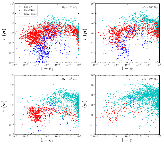
Figure 1: The output inner eccentricity and lifetime of the BBHs (inspiralling time from when gravitational wave decay dominates the evolution of the inner orbit to the moment of the final coalescence) of model MP1 given different MBH masses. For clarity, only $3000$ samples are shown in each panel. The colored dots show the dynamical process experienced by the BBHs before merging: the KL oscillation (red dots), encounters with a background object (cyan dots) and with the MBH (blue dots).

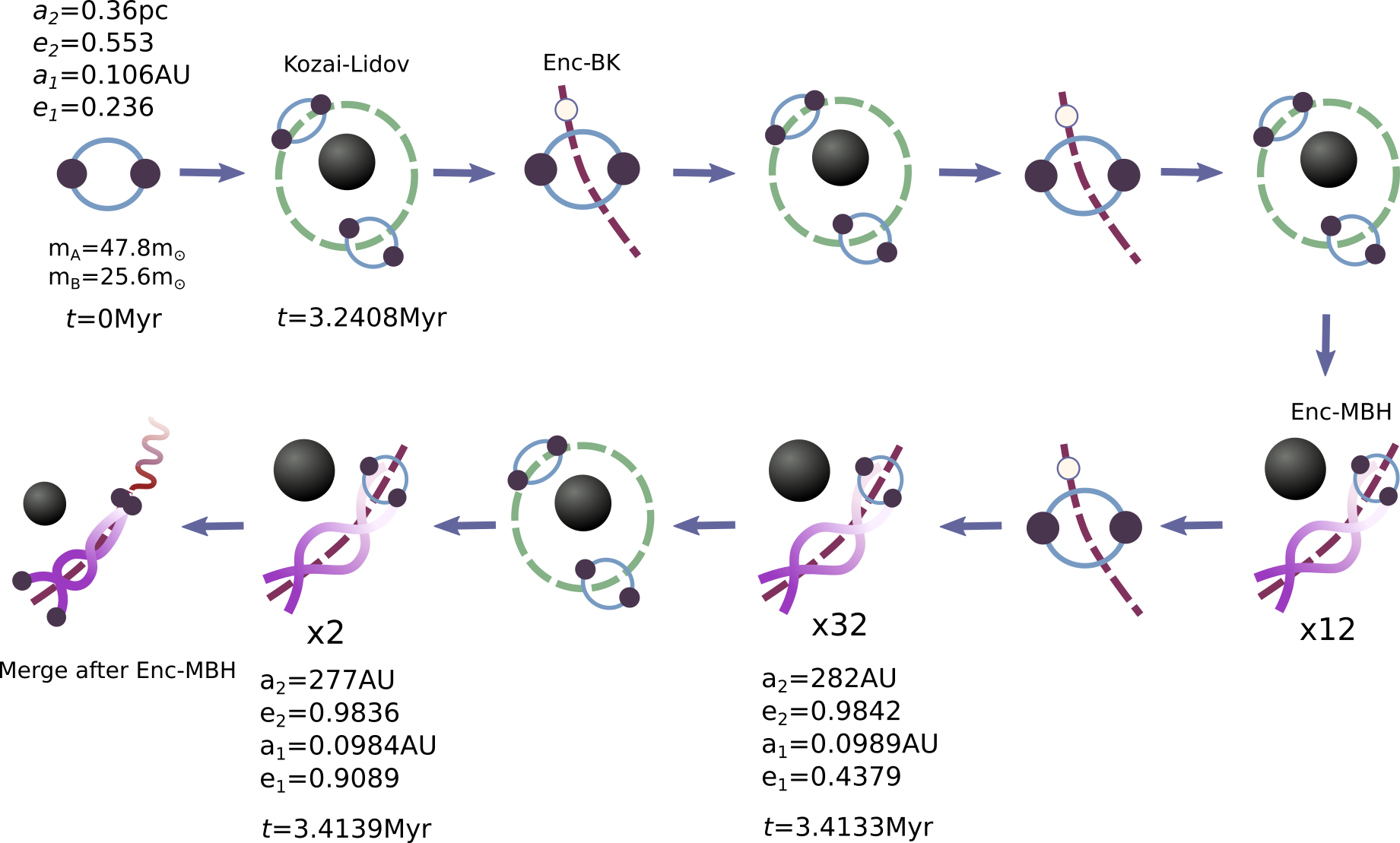
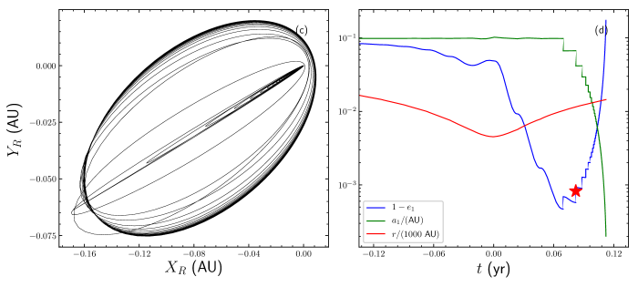
Figure 2: Upper illustrations show one example of the dynamical evolution of a BBH that finally merge due to an encounter with the MBH. The example is from model MP1 of simulation runs given $M_{\bullet}=10^{5}M_{\odot}$. “Kozai-Lidov”, “Enc-MBH”, and “Enc-BK” in the illustration show the dynamical process of KL oscillation, an encounter with the MBH, and an encounter with a background object, respectively. The trajectory of the relative position vector between the two components of the BBH during the final encounter with the MBH is shown in the bottom left panel. The evolution of the SMA ($a_{1}$), eccentricity ($e_{1}$) of the inner orbit of BBH and the distance $(r)$ of the mass center of BBH to the MBH during the final encounter with the MBH are shown in the bottom right panel. The red star in the eccentricity curve marks the position where the GNC find that the GW orbital decay dominates the evolution of the inner orbit of the BBH.

In each simulation, BBHs form continuously, and the distribution of BBHs dynamically evolve into an equilibrium state when the density profile of BBHs is converged at any position of the cluster. During a time interval ${\Delta}t$, suppose that there are a number of ${\Delta}N_{\rm tot}$ BBHs generated in the simulation, and a number of ${\Delta}N_{\rm mrg}$ of samples end up with merging, then we can estimate that the corresponding merging fractions of BBHs are given by $f_{\rm mrg}={\Delta}N_{\rm mrg}/{\Delta}N_{\rm tot}$. Similarly, we can obtain the fraction of BBHs end up with tidal disruption $f_{\rm td}$ and ionization due to the encounters with the background objects $f_{\rm ion}$. These fraction of BBH are shown in Table 2.

2.3.1 The Merging samples

We find that in galactic nulcei, typically $f_{\rm mrg}\sim 3-40\%$ of the BBHs end up with merging events (See Table 2). The highest fraction occur in clusters with MBHs around $M_{\bullet}\sim 10^{6}M_{\odot}$ and usually decrease for larger or smaller MBHs. When the inner orbit of a BBH in the numerical simulation is found dominated by GW radiation, the simulation ends and it is output from the GNC. Usually the BBHs samples output from the simulations are with very different distributions of eccentricities and lifetimes . The results of MP1 are shown in Figure 1 as an example.

We found that these events have two unique features. The first one is that they have very significant eccentricities. As shown in Table 2, about $40\%\sim 70\%$ of them have extremely high eccentricities ($1-e_{1}\mathrel{\mathchoice{\lower 4.0pt\vbox{\halign{$\nms\displaystyle\hfil#\hfil$\cr<\crcr\sim\crcr}}}{\lower 4.0pt\vbox{\halign{$\nms\textstyle\hfil#\hfil$\cr<\crcr\sim\crcr}}}{\lower 4.0pt\vbox{\halign{$\nms\scriptstyle\hfil#\hfil$\cr<\crcr\sim\crcr}}}{\lower 4.0pt\vbox{\halign{$\nms\scriptscriptstyle\hfil#\hfil$\cr<\crcr\sim\crcr}}}}10^{-3}$). The other one is that some of the events can happen at positions very close to the MBH. For example, up to $10\%$ of all BBHs can merge at distance $r$ from the MBH, or with SMA of the outer orbit $a$ smaller than $10^{4}r_{\rm SW}$. Up to $30\%$ of all merging events are with pericenter of the outer orbit $r_{p2}<10^{4}r_{\rm SW}$. Here $r_{\rm SW}$ is the Schwarzschild radius.

These merging BBHs can be either happens (1) After one or multiple encounters with the MBH (the fraction of which is denoted by $f_{\rm mrg}^{\rm eMBH}$). (2) after Kozai Lidov oscillation (denoted by $f_{\rm mrg}^{\rm KL}$); (3) after one encounter with a background object (denoted by $f_{\rm mrg}^{\rm eBK}$); Here $f_{\rm mrg}^{\rm eMBH}$, $f_{\rm mrg}^{\rm KL}$, and $f^{\rm eBK}_{\rm mrg}$ are all obtained by counting over the merging BBHs.

A significant fraction (up to $f_{\rm mrg}^{\rm eMBH}\sim 25\%$) of all merging BBHs are merged after one or multiple encounters with the MBH. These events happen more likely around MBHs of $10^{5}M_{\odot}$. Before such encounter, the BBHs have usually experienced multiple encounters with background objects, epochs of KL oscillations and also encounters with the MBH. One example of such dynamical evolution is shown in Figure 2. The eccentricity of the inner orbit of BBH is cumulatively excited from initial value of $e_{1}=0.236$ to $\sim 0.9$ before the final dramatic encounters with the MBH that lead to the merging event. The bottom panels of Figure 2 show the trajectory (bottom left) and the evolution of both the inner and outer orbits (bottom right) right before the merging of the BBH.

The encounter of BBHs with MBH can excite the BBHs into extremely high eccentricities, i.e., up to $1-e_{1}\simeq 10^{-2}-10^{-6}$ (See Figure 1). For a few of them ($\sim 1\%$), the eccentricity is so high that the BBH will plunge directly to each other with pericenter about a few times of horizon (which is a few to several tens of km), result in an rapidly decay GW transit event; Mainly due to their high eccentricity, they can merge very quickly after the encounter with the MBH. Figure 1 show that the lifetime of the majorities of these events are $10^{3}$s$\sim 10^{3}$yr, the short ones of which merge within days right after the encounter.

The relatively short lifetime of these events are understandable, as otherwise, in most cases, they will be modified again by a successive encounter with the MBH. Thus, the period of the outer orbit of BBHs can set an upper limit of their GW lifetime. As a result, the lifetime of these events will be slightly longer if the mass of MBH is larger, e.g., $10^{7}M_{\odot}$, as shown in bottom left panel of Figure 1.

Another important feature is that these events merge very close to the central MBH. The merging event usually happens right after the encounter. For $M_{\bullet}=10^{5}M_{\odot}$, the pericenter of the encounter can be about a few AU (See the bottom right panel of Figure 2), and the merging position is at distance of about a few tens of AU from the black hole ($\sim 10^{4}r_{\rm SW}$ for $M_{\bullet}=10^{5}M_{\odot}$). As these events happen very close to the MBH, the phases of GW will be significantly drifted due to the acceleration. We will discuss about them later in Section 5.

Note that the merging of a BBH is usually a result of multiple encounters with the MBH. As the outer orbit of a BBH is dynamically evolving under the two-body and resonant relaxations, a BBH will experience multiple encounters (which can be up to hundreds and thousands) with the MBH when it moves from $D=r_{p}/r_{\rm td}\sim 3$ into $D\sim 1$ before being tidally disrupted, where $r_{td}$ is the tidal radius of the BBH. For example, the BBH illustrated in Figure 2 is merged after in total of $45$ times of encounters with MBH. The probability of a BBH with inital eccentricity $e_{1}<0.9$ merging after encountering with MBH with $D<3$ is usually $0.01\%-0.1\%$ per encounter. In most cases the BBH will remain integrity after that although the inner orbital eccentricity is changed. Thus, the probability of merging is dramatically increased due to the excited inner eccentricity of the BBH and the increased number of encounters.

Another important merging channel of BBHs is the KL oscillation, of which the fraction to all the merging events can be up to $\sim 70\%$, and decrease to $\sim 6-16\%$ with increasing mass of MBH. Similarly, KL and other dynamical processes have been cumulatively modified the BBHs before the last KL oscillation that leads to the final merging event. One example of such evolution is illustrated in Figure 3. The panel on the right of Figure 3 show the evolution of the inner orbit of BBHs before the final merging event. The GNC output the eccentricity of this event with $e_{1}\sim 0.97$ when GW dominates the evolution of the inner orbit. As shown in Figure 1, the output eccentricity of BBHs due to KL can be up to $1-e_{1}\sim 10^{-7}$, comparable to those due to BBH-MBH encounters. The lifetime of these events are about a few hours up to $10^{5}$ yr, slightly depends on the mass of the MBH.

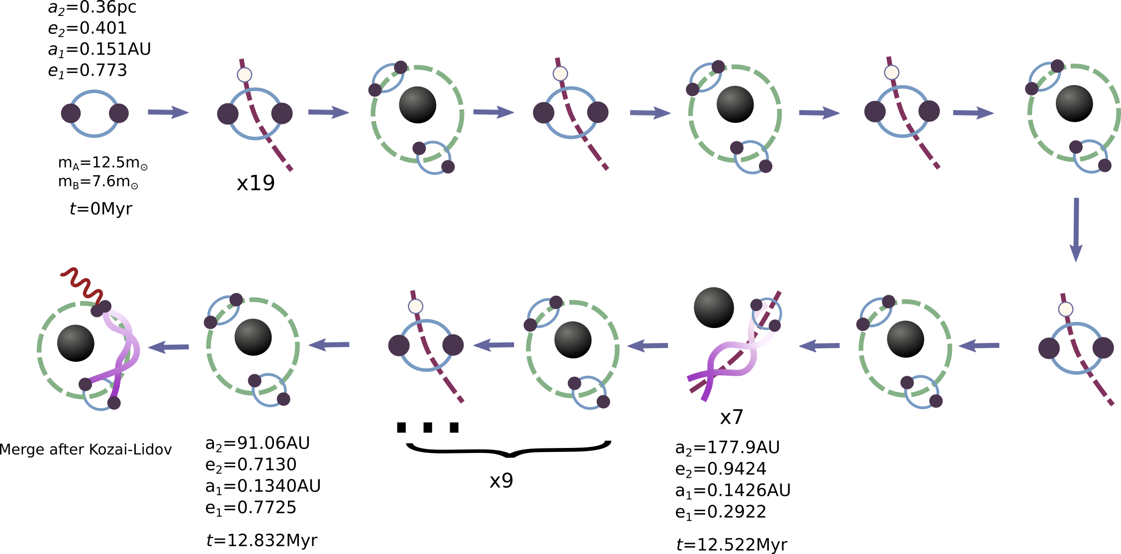
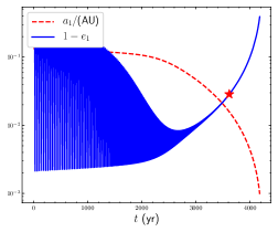
Figure 3: The illustrations on the left show one example of the dynamical evolution history of a BBH that merge due to KL oscillation. The example is from model MP1 of simulations runs given $M_{\bullet}=10^{5}M_{\odot}$. The illustration of each dynamical processes are similar to Figure 2. The orbital evolution of the inner orbit of BBH during the final KL oscillation are shown in the panel on the right. The red star in the eccentricity curve marks the position where the GNC find that the GW orbital decay dominates the evolution of the inner orbit of the BBH.

The encounters with the background objects is the third merging channel of BBHs, the fraction of which varies between $7.0\%\sim 90\%$ of all merging events. The rates are higher if increasing the mass of the MBH. The resulting eccentricities are relatively smaller compared to the first two channels mentioned above, i.e., $1-e_{1}=10^{-4}-1$ (See Figure 1). The lifetime of these events can be up to $10^{4}$yrs around $10^{5}M_{\odot}$ MBH or up to $10^{7}$ yrs around $10^{8}M_{\odot}$ MBH. In most cases, such a long time is limited by the dynamical timesteps $\delta t$ of GNC as we require that the merging timescale of these BBH samples satisfy $t_{\rm GW}<0.1\delta t$. Here $\delta t$ is set according to the timescales of two body relaxation, resonant relaxation, or the collision rate between BBHs and the background objects. For more details, see Paper I.

The overall merging rates in the local universe can be estimated according to Equation 2, and the results can be seen in Table 2. We find that the rate mainly depend on the assumed background masses of the stars. For models assuming $m_{\star}=1$ (models MP1-3 and MP5), the estimated rates are $5-200$Gpc^-3yr^-1. If the background mass is $m_{\star}=10M_{\odot}$ (model MP4), the rate reduce to $0.2-1.7$Gpc^-3yr^-1. When the background mass is mixing stars and stellar black holes (in model MP6), the rate is between the above two, i.e., $7-71$Gpc^-3yr^-1. Thus, all models except MP4 are consistent with the rate given by aLIGO/Virgo detection, which is $\sim 23.9$Gpc^-3yr^-1(Abbott et al., 2021). As the number and masses should be dominated by main-sequence stars over the entire cluster except the very inner regions  (Alexander, 2005), MP4 should be unfavored by the observations.

2.3.2 The tidally disrupted or ionized samples

The BBHs may also end up with tidal disruption by close encounters with the MBH or be ionized due to encounters with the background objects. $f_{\rm td}$ can be very significant near small mass MBH ($\sim 60\%$) and decreased to $\sim 7\%$ for MBH with $10^{8}M_{\odot}$. This is because in small mass MBH, the two body and resonant relaxation dynamical timescale is much shorter, making them more easily move into the loss cone region. The fraction of ionization of BBHs is low, i.e., $f_{\rm ion}\sim 1-7\%$, if the masses of the background stars are small (e.g., MP1-3 and MP5). However, $f_{\rm ion}\sim 10-20\%$ if the background stars’ masses is $m_{\star}=10M_{\odot}$ (for MP4), and $f_{\rm ion}\sim 5-11\%$ if the background objects mix with single stars and black holes. These results suggest that the tidal forces of the MBH, rather than the encounters with the background stars, is more effective in destroying the binarities of black holes in the vicinity of MBH.

3 Observing BBHs in current and future GW observatories

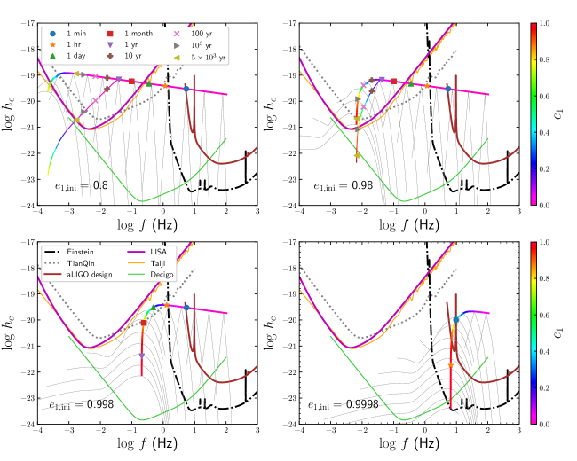
Figure 4: The evolution of the strain amplitude $h_{c}$ for BBHs with different eccentricities. BBHs start with orbital period $P_{1,\rm ini}=1$day and with different eccentricity ($e_{1,\rm ini}$ in each panel). For illustration purpose, all BBHs are with $m_{A}=m_{B}=20M_{\odot}$ and $z=0.01$. The noise-level of different GW observatories are shown in lines with different color and styles, see the legends in the lower right panel. The thin gray lines show the GW spectrum at different harmonics. The thick (or thin) solid lines are the evolution of the peak of the GW radiation (or assuming that the BBHs have no frequency evolution in a $t_{M}=5$ yr’s mission, see texts in Section 3 for more detail), of which the color map show the eccentricity ($e_{1}$) of the BBHs during the evolution.

In this section, we investigate how the merging BBHs obtained by GNC described in Section 2 appear in the current (aLIGO/Virgo O2) and future GW observatories, i.e., aLIGO (design), Einstein, DECIGO, TianQin, LISA and Taiji observatories. We mainly focus on the evolution and harmonics of the BBHs appeared in the observations (Section 3.1), and we investigate the numbers and SNR of the inspiralling and merging of BBHs (Section 3.2 and Section 3.3).

3.1 The evolution of BBHs and the harmonics of GW

As shown in Section 2.3 and Figure 1, BBHs form in galactic nuclei around MBH usually have very significant eccentricities, thus their GW spectrum will spread to high orders of harmonics. For each of the BBH merging events from our simulation, we can get their orbital evolution under GW orbital decay and also the characteristic strain of GW at the $n$th harmonic before coalescence, which is given by (Barack & Cutler, 2004) (See also Randall et al (2021) for a more efficient way of estimation.)

$$h_{c,n}(f)=\frac{1}{\pi D}\sqrt{\frac{2G}{c^{3}}\frac{dE_{n}}{df_{r}}}$$ (3)

Where $D$ is the comoving distance of the BBH. The detail forms of $dE_{n}/df_{r}$ can be found in the literature (e.g., Huerta et al., 2015; Chen et al., 2017; Peters & Mathews, 1963). We summarize them in the Appendix B.

The SNR is then given by (O’Leary et al., 2009)

$$\rho^{2}=\left(\frac{\rm S}{N}\right)^{2}=\sum^{n_{\rm max}}_{n=1}\int^{f_{\rm max}}_{f_{\rm min}}\frac{h_{c,n}^{2}(f)}{fS(f)}\frac{df}{f}$$ (4)

where $f=f_{0}(1+z)$ and $f_{0}$ is the frequency of the GW in the rest frame and in the observer’s frame, respectively; $S(f)$ is the strain spectral sensitivity of the observatory. For aLIGO/Virgo(O2) and aLIGO(design) sensitivity, it is given by Barsotti et al. (2012) and Barsotti et al. (2018), respectively. For LISA $S(f)$ is given by Robson et al. (2019), Einstein by Hild et al. (2011), DECIGO by Yagi & Seto (2011), TaiJi by Ruan et al. (2020) and TianQin by Luo et al. (2016); Wang et al. (2019).

The integrations are performed between the minimum and maximum frequency of the BBHs during the mission, and they depend on the order of harmonic $n$. For a given BBH, if the minimum and maximum of GW frequency at $n$-th harmonic in a five years mission is given by $f_{{\rm min},n}$ and $f_{{\rm max},n}$, respectively, the minimum and maximum frequency of the observational band are given by $f_{\rm min,ob}$ and $f_{\rm max,ob}$, respectively, then the lower and upper limit for the integration is given by $f_{\rm min}={\rm max}(f_{{\rm min},n},f_{\rm min,ob})$, $f_{\rm max}={\rm min}(f_{{\rm max},n},f_{\rm max,ob})$, respectively.

The duration and evolution of the GW of a BBH observed in an observatory depend largely on its eccentricity. Figure 4 illustrates some of the examples of BBH’s $f-h_{c}$ evolution. For a BBH starts with $P_{1,\rm ini}=1$day, and $e_{1,\rm ini}=0.8$, the strains enter into LISA band when its eccentricity decreases to $e_{1}\sim 0.4$, and then stay in LISA band for thousands of years before merging. Most of these events will be considered as background sources in LISA band as they evolved too slowly unless they have significant SNR. For these BBHs with almost no frequency evolution, Equation 4 become $\rho^{2}\simeq\sum h^{2}_{c,n}(\dot{f}t_{M}/f)/(fS(f))$, where $t_{M}$ is the mission time. Thus, when $t_{M}<f/\dot{f}$, we can approximately consider that the BBHs have no evolution in frequency, and the quantity $h_{c,n}\sqrt{\dot{f}t_{M}/f}=h(f)ft_{M}$ (thin solid line with colormap in Figure 4) provides an effective characteristic amplitude that can be used in estimating SNR, where $h(f)$ is the amplitude of the GW (Finn & Thorne, 2000; D’Orazio & Samsing, 2018; Robson et al., 2019; Sesana et al., 2005).

If the eccentricity is higher, i.e., $e_{1,\rm ini}=0.98$, the strain amplitude rise above the noise level of LISA with slightly increased GW frequency when $e_{1}\sim 0.8$, and then moves towards Einstein and aLIGO band after evolving about a thousand years. If $e_{1,\rm ini}=0.998$, the evolution become much faster and the peak arises directly into the band of TianQin, without passing through LISA band, and then move into Einstein and aLIGO band within one month. If a BBH has an even higher eccentricity of $e_{1,\rm ini}=0.9998$ ($1-e_{1,\rm ini}\sim 10^{-4}$), its characteristic strain can directly rise above and into Einstein and aLIGO band. These results suggest that for very highly eccentric BBHs, they can only be seen in detectors with entering frequencies larger than $0.1\sim 1$ Hz (e.g., aLIGO, Einstein or DECIGO detectors).

3.2 Generating samples of inspiralling/merging BBHs

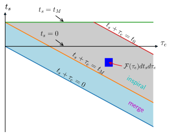
Figure 5: Figure show the timeline of the generation and the merging of samples. $t_{s}$ is the time where sample forms and $\tau_{e}$ is the lifetime of each sample observed on earth. The observation starts at $t_{s}=0$ and ends at $t_{s}=t_{M}=5$ yr. The samples with $t_{s}<-\tau_{e}$ are already coalesced before the start of the mission, and those form between $-\tau_{e}<t_{s}<t_{M}-\tau_{e}$ filled by color light blue are samples coalescing during the mission. The regions filled by light grey are samples insprialling with time of coalescence $t_{\rm CO}$ less than a given time of interest $t_{0}$ during the mission. $\mathcal{F}(\tau_{e})$ is the formation rate of samples with lifetime $\tau_{e}$ given by Equation 5.

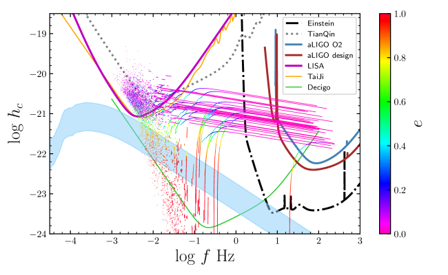
Figure 6: The $5$yr evolution of the strain amplitude of inspiralling BBHs from a MC realization described in Section 3.2, by using samples of MP1 (in total of $5000$ samples are presented as examples). For clarity of the figure, here we only show samples with $0.001<z<0.5$, and with time to coalescence at the start of the observation less than $10^{3}$ yr. The solid lines with color maps are the evolution of the peak of the GW radiation. The color map in the solid line show the eccentricity $e_{1}$ of the BBHs during the evolution. The light-blue shaded region show the characteristic strain noise amplitude of the GW background from BBHs merging around MBHs. For more details of the GW background, see Section 6.

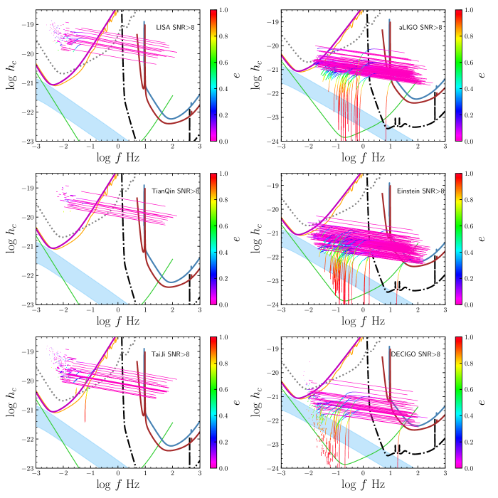
Figure 7: Examples of the evolution of BBHs with SNR$>8$ in LISA, aLIGO (design), TianQin, Einstein, TaiJi and DECIGO during a continuous $5$ yr mission. The solid lines with color maps are the evolution of the peak of the GW radiation. The color map in the solid line show the eccentricity $e_{1}$ of the BBHs during the evolution. The samples are limited with redshifts of $0.001<z<2$.

Section 2.2 and Table 2 provide the merging rates of BBHs in the local universe. These numbers are related to the final stage of the merging BBHs, thus usually useful for aLIGO/Virgo detection. However, LISA or other low frequency detectors can probe the inspiralling phase of BBHs. The number of inspiralling BBHs detected in the different observatories should depend on the mission time ($5$ yr in this work), the evolution trajectories of $f-h_{c}$ of the individual BBHs, the detection sensitivity of observatories, and etc.

In order to investigate the inspiralling samples that can be observed in individual or mulitiple observatories, first we need to estimate the number of inspiralling/merging BBHs given some distribution of their lifetime (defined in Section 2.3.1) and then generate a group of Monte-Carlo samples for SNR estimation. The details are in the following sections.

3.2.1 Estimating the total number of inspiralling/merging BBHs

Suppose that we have a group of samples resulting from a simulation by GNC given MBH mass of $M_{\bullet}$, and denote the local lifetime of samples from the simulation by $\tau$ (The time span of a BBH from when GW dominate its inner orbital evolution to its final coalescence, see also Figure 1), then the formation rate of samples with $\tau\rightarrow\tau+{\rm d}\tau$ is given by $\mathbf{R}({M_{\bullet}},\tau){\rm d}\tau=\mathbf{R}(M_{\bullet})f(\tau|M_{\bullet}){\rm d}\tau$, where $f(\tau|M_{\bullet})$ is the probability distribution function (pdf) of $\tau$ from the simulation given MBH mass of $M_{\bullet}$ and $\mathbf{R}(M_{\bullet})$ can be estimated by Equation 1. The formation rate of BBHs observed per unit time of earth with per unit lifetime $\tau_{e}=(1+z)\tau$ observed on earth, is given by integrating over all MBHs and all redshift:

$$\mathcal{F}(\tau_{e})=\int_{0}^{\infty}\frac{n(M_{\bullet},z)}{(1+z)^{2}}R\left(M_{\bullet},\frac{\tau_{e}}{1+z}\right)dM_{\bullet}\int_{0}^{\infty}\frac{dV_{c}}{dz}dz$$ (5)

where $n(M_{\bullet},z)$ is the black hole number density per unit comoving volume given by Aversa et al. (2015), and $V_{c}$ is the comoving volume. Then the number of BBH samples formed measured at earth time $t_{s}\rightarrow t_{s}+dt_{s}$ with lifetime between $\tau_{e}\rightarrow\tau_{e}+d\tau_{e}$ is given by $\mathcal{F}(\tau_{e})dt_{s}d\tau_{e}$ . Note that here $t_{s}$ is the formation time of BBHs observed on earth (the moment when the evolution of inner orbit of BBH is dominated by GW radiation). Here we consider redshift between $0.001<z<2$.

The formation and coalescence timeline of samples with different $\tau_{e}$ can then be illustrated in Figure 5. Suppose that $t_{s}=0$ is the time when the observation starts, then samples form before $t_{s}\leq-\tau_{e}$ coalesce at time $t_{s}\leq 0$, right before the start of the mission. Those form between $-\tau_{e}<t_{s}<t_{M}-\tau_{e}$ will coalesce during the mission, where $t_{M}$ is the mission time. If the time to coalescence of a BBH measured at the start of the mission is denoted by $t_{\rm CO}$, then the number of samples merging, or inspiralling with $t_{\rm CO}$ less than a time of interest $t_{0}$, i.e., $t_{\rm CO}<t_{0}$ ($t_{0}=1000$yr, see texts later) can be obtained by :

$$N_{\rm tot} (t_{\rm co}<t_{0}|t_{M})=N_{\rm merge}(t_{M})+N_{\rm insp}(t_{\rm co}<t_{0}|t_{M})$$ (6)

where $N_{\rm merge}$ is the number of merging samples during the mission, and $N_{\rm insp}$ is the number of insprialling samples with time to coalescence $t_{\rm CO}<t_{0}$ at the start of the mission. According to Figure 5, they can be estimated by

$$N_{\rm merge} =t_{M}\int^{\infty}_{0}\mathcal{F}(\tau_{e})d\tau_{e}$$ (7)

$$N_{\rm insp} =\int^{t_{0}-t_{M}}_{0}\tau_{e}\mathcal{F}(\tau_{e})d\tau_{e}+t_{0}\int^{\infty}_{t_{0}-t_{M}}\mathcal{F}(\tau_{e})d\tau_{e}$$

From Figure 4, we can see that most BBHs appeared in LISA band usually have a lifetime of $\mathrel{\mathchoice{\lower 4.0pt\vbox{\halign{$\nms\displaystyle\hfil#\hfil$\cr<\crcr\sim\crcr}}}{\lower 4.0pt\vbox{\halign{$\nms\textstyle\hfil#\hfil$\cr<\crcr\sim\crcr}}}{\lower 4.0pt\vbox{\halign{$\nms\scriptstyle\hfil#\hfil$\cr<\crcr\sim\crcr}}}{\lower 4.0pt\vbox{\halign{$\nms\scriptscriptstyle\hfil#\hfil$\cr<\crcr\sim\crcr}}}}10^{3}$yr. Thus, by setting $t_{0}=1000$yr is sufficient in covering most BBHs that can be detected with high SNR in ground and space-based observatories. We found that for models in Table 1, in a $5$ yr mission, the typical number of $N_{\rm tot}(t_{\rm co}<10^{3}{\rm~{}yr})\sim 10^{6}$.

The total number of inspiralling samples at any given moment are given by $t_{M}\rightarrow 0$ and $t_{0}\rightarrow\infty$, which can be further reduced to

$$N_{\rm tot}=\int^{\infty}_{0}R(M_{\bullet},\tau)\tau d\tau\int^{\infty}_{0}dz\int^{\infty}_{0}dM_{\bullet}n(M_{\bullet},z)\frac{dV_{c}}{dz}$$ (8)

We find that the typical number for all models is $N_{\rm tot}\sim 10^{9}$. Most of these sources should be very slowly evolving and contributing to a background of GW. The amplitude of the GW backgrounds contributed from BBHs merging around MBH will be discussed later in Section 6.

3.2.2 Generating the inspiralling/merging samples by Monte-Carlo method

We use a Monte-Carlo (MC) method to generate the mock inspiralling/merging samples during a given time of mission $t_{M}$ and with time to coalescence less than $t_{0}$. Statistical analysis of these samples can then provide predictions of the inspiralling/merging samples for different models. Each of them is generated following the steps below:

1. Draw a pair of $M_{\bullet},z$ from a two-dimensional distribution given by

   $$P(M_{\bullet},z)\propto n(M_{\bullet},z)\frac{\mathbf{R}(M_{\bullet})}{1+z}\frac{dV_{c}}{dz}$$ (9)

2. For a $M_{\bullet}$ from above, get the samples from the simulation runs of GNC given MBH mass closest to $M_{\bullet}$ (one of the $M_{\bullet}=10^{5}M_{\odot},10^{6}M_{\odot},10^{7}M_{\odot}$ and $10^{8}M_{\odot}$). Randomly select one of the samples, get its corresponding lifetime observed on earth, i.e., $\tau_{e}=\tau(1+z)$. According to Figure 5, suppose that the mission last for $t_{M}=5$ yr, and we are only interested for samples with time of coalescence less than $t_{0}=1000$yr at the start of observation, then the probability of accepting this sample with lifetime $\tau_{e}$ is $\propto{\rm min}[1,(t_{M}+\tau_{e})/t_{0}]$. If the sample is rejected, then go back to step (1).

3. The formation time of this sample observed on earth ($t_{s}$) is uniformly distributed between $(-\tau_{e},t_{0}-\tau_{e})$ if $\tau_{e}>t_{0}-t_{M}$, or between $(-\tau_{e},t_{M})$ if $\tau_{e}<t_{0}-t_{M}$.

4. At the start of the mission, if $t_{s}<0$, the time of coalescence of each sample is given by $t_{\rm co}=(t_{s}+\tau_{e})$; If $t_{s}>0$, they are newly formed samples and their time of colascences is given by $t_{\rm co}=\tau_{e}$.

Such process repeats until a sufficiently large number of Monte-Carlo samples are realized. The orbital evolution of these samples due to GW orbital decay are then calculated and the frequency and the strain amplitude of GW are estimated according to Equation 3

Figure 6 show the $5$ yr evolution of $5000$ examples resulting from above MC simulation for model MP1. We can see that in LISA/TaiJi band, many of the BBHs inspiral at frequency $1\sim 10$mHz do not show significant evolution during the mission time. Only samples above $10\sim 100$mHz show some evolution towards high frequencies. The eccentricities of a number of BBHs are so high that, the $h_{c}$ rise up at frequency $\sim 0.1$Hz and directly evolved into Einstein and aLIGO/Virgo band without passing through any of the space-based observatories such as LISA/TianQin/TaiJi. We expect that such a rising phase of $h_{c}$ can only be probed by DECIGO (see also Chen & Amaro-Seoane, 2017), that are sensitive to frequencies between $0.1-10$Hz (Arca Sedda et al., 2019; Liu et al., 2020a).

3.3 The SNR of BBHs

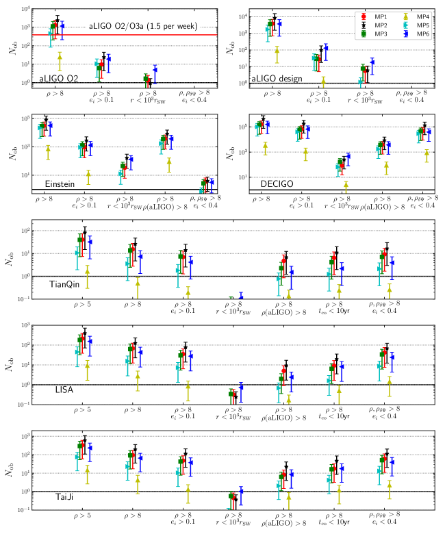
Figure 8: Predicted numbers of inspiralling/merging BBHs in different observatories given SNR $\rho>8$ (or $\rho>5$) and also some other conditions. For example, with entering eccentricity $e_{i}>0.1$, or inspiralling/merging at distance of $r<10^{3}r_{\rm SW}$ ($r_{\rm SW}$ is the Schwarzchild radius) to the MBH, or with the SNR of the Doppler drift of phase $\rho_{\delta\Psi}>8$ (See Equation 13) and with $e_{i}<0.4$, or with time to coalescence at the start of mission less than ten years ($t_{\rm co}<10$yr). We also predict number of BBHs that can be observed in multiband observations. For example, we show the number of samples with $\rho>8$ in Einstein, LISA, TianQin and TaiJi and also with SNR$>8$ in aLIGO(design) band ($\rho(\rm aLIGO)>8$). Symbols for each model show the mean value of the prediction and the errorbar is from the uncertainty of the event rates.

Here we mainly focus on BBH merging samples with SNR$>8$ such that the false alarm rate is below $0.02$ (Abbott et al., 2016e). Figure 7 show some examples of those BBHs with SNR$>8$ in different observatories. We can see that in LISA and TianQin (TaiJi is also similar), many inspiralling BBHs show little evolution in frequency while others will evolve quickly and can be also detected in Einstein or aLIGO band. In these space-based observatories, some of the highly-eccentric BBHs evolve differently in $f-h_{c}$ spaces from those of near circular ones. For BBHs with SNR$>8$ in Einstein or aLIGO band, many of them are not previously detectable in LISA/TaiJi/TianQin band. For most samples, their GW radiation can be continuously monitored by DECIGO, suggesting that DECIGO will be an ideal observatory to trace the inspiralling and merging of these highly eccentric BBH mergers.

The number of samples with SNR$>8$ in different observatories can be estimated as follows. Suppose that by using Monte-Carlo method described in Section 3.2, a total number of $N_{\rm mc}$ is generated and among them there are a number of $N_{\rm ob,mc}$ samples with SNR$>8$, then the number of samples in reality is given by $N_{\rm ob}=N_{\rm ob,mc}/N_{\rm mc}\times N_{\rm tot}(t_{\rm CO}<1000{\rm yr}|t_{M}=5{\rm yr})$, where $N_{\rm tot}(t_{\rm CO}<1000{\rm yr}|t_{M}=5{\rm yr})$ is estimated according to Equation 6. The observable number of BBHs under other conditions is also estimated similarly by the method above. In a five-years mission, the total number of BBHs that can be observed with SNR$>8$ in different observatories, or under other conditions, can be found in Figure 8.

If using the current aLIGO/Virgo facility and observing for $5$ yrs, we found that about $N_{\rm ob}\sim 10^{2}-10^{3}$ BBHs mergers with SNR$>8$ can be detected. This number is well consistent with the number of $1.5$ per week from the current LIGO-O2 and LIGO-O3a surveys (Abbott et al., 2021) (See the red horizontal line of the top left panel in Figure 8). If aLIGO/Virgo can upgrade to the designed aLIGO in the future, the expected numbers can be about ten times higher, i.e., $10^{3}-10^{4}$ with SNR$>8$ in a five year’s mission. The number of merging events with SNR$>8$ in both Einstein and DECIGO can be up to $\sim 10^{5}$. Note that here the upper limit of redshift is $z<2$. If we consider higher redshift samples, the number of observable samples for both Einstein and DECIGO is expected much higher.

The total number of SNR$>8$ events in LISA/TaiJi band can be up to $\sim 200/300$. The number become $\sim 10^{3}$ if requiring SNR$>5$. For TianQin, the numbers of BBHs with SNR$>8$ (SNR$>5$) is about $1-50$ ($10\sim 200$), mainly due to their high noise level.

Some of the inspiralling BBHs in LISA/TianQin/TaiJi have a short time to coalescence (e.g.,$t_{\rm CO}<10$yr), and them will further evolve into and merging in Einstein/aLIGO band. These samples are interesting for multiple band observations of the same inspiralling event. However, because some of the BBHs have very significant eccentricities, not all of those that enter into aLIGO or Einstein band have previously detectable in LISA/TaiJi/TianQin band. For example, the characteristic strain amplitude of many of these BBHs rise above $10^{-21\sim-22}$ at $f\sim 0.1-1$Hz, which is far below the sensitivity of LISA/TaiJi. Only a fraction ($\sim 20\%$) of the BBHs inspiralling in LISA/TaiJi/TianQin band can enter into the aLIGO(design) band with SNR$>8$. The total number of BBHs that enter into both bands of LISA-aLIGO, TaiJi-aLIGO, or TianQin-aLIGO can be up to $\sim 20$, $\sim 50$, or $\sim 50$ in a five years’ mission, respectively.

4 The entering eccentricity of BBHs in different observatories

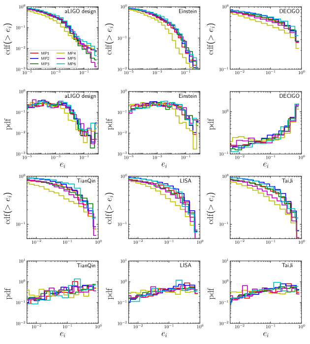
Figure 9: The cumulative distribution function (cdf) or probability distribution function (pdf) of the eccentricity distribution of inspiralling/merging BBHs with SNR$>8$ in different observatories and in different models.

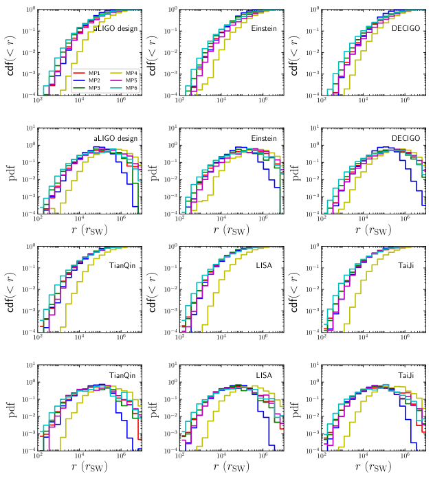
Figure 10: The cdf (top panels) or pdf (bottom panels) of the distance of the inspiralling/merging BBHs from the central MBHs (in unit of $r_{\rm SW}$), which can be detected in GW observatories with SNR$>8$.

The eccentricity of BBH is one of the most important features that can be used to distinguish different formation scenario of BBHs (Wen, 2003; Hoang et al., 2018; Antonini & Perets, 2012; Zhang et al., 2019; Seto, 2016; Kyutoku & Seto, 2016; Nishizawa et al., 2016; Breivik et al., 2016). Here we define the “entering eccentricity” (denoted by $e_{i}$) of a BBH in a given observatory as follows. At the start of mission, if the peak of characteristic strain $h_{c}$ is below the noise level, then $e_{i}$ is the inner eccentricity ($e_{1}$) of BBH when $h_{c}$ rise and cross (for the first time) the noise level of an observatory. If initially $h_{c}$ is above the noise level and the GW frequency $f$ is within the band of observation, then $e_{i}=e_{1}$ when the mission starts ($t_{s}=0$). Here we investigate the entering eccentricity ($e_{i}$) for samples that is with SNR $\rho>8$. The fraction and the number of eccentric insprialling/merging BBHs with $e_{i}>0.1$ and $\rho>8$ for different observatories are shown in Table 3 and in Figure 8, respectively. The distribution of the entering eccentricity in different observatories can be found in Figure 9.

We find that the pdf of $e_{i}$ is nearly uniformly distributed between $\sim 0.1-1$ (in log scale) for LISA/TaiJi/TianQin. For DECIGO, however, the pdf of $e_{i}$ peaks around $\sim 0.9$, as it can cover the rising phase of those extremely eccentric BBHs. For these space-based observatories, the fraction of eccentric events ($e_{i}>0.1$) is $\sim 30-70\%$. In a five year’s mission, the expected number of samples with SNR$>8$ and $e_{i}>0.1$ are up to $\sim 10^{5}$, $\sim 100$, $\sim 200$ and $\sim 30$ for DECIGO, LISA, TaiJi and TianQin, respectively.

For the ground-based observatories, the peak of pdf is much smaller. For example, the peak of pdf is around $e_{i}\sim 10^{-3}$ for aLIGO band, $\sim 10^{-2}$ for Einstein band. The fraction of $e_{i}>0.1$ is low for aLIGO(O2)/ aLIGO(design) ($\sim 1-2\%$) and Einstein ($\sim 2-5\%$) among all the detectable events, simply because their observational windows are at high frequency. The expected number of events with SNR$>8$ and $e_{i}>0.1$ are about $1-10$ for aLIGO(O2), $10-100$ for aLIGO(design) and $\sim 10^{3}$ for Einstein. Thus they should not be rare events.

In some cases, the eccentricities of these events in aLIGO/Einstein band are quite significant, e.g., $e_{i}>0.3$, such that they rise above the noise level at GW frequency of about tens of Hz. For example, In Figure 6, the peak of GW radiation of one highly eccentric event rises above the noise level of aLIGO directly at $f\sim 20$Hz with $e_{i}\sim 0.5$. Similarly in the bottom right panel of Figure 7, one high eccentricity events rise above the noise level of Einstein at $f\sim 20$Hz. These BBHs will merge very quickly without passing through LISA band or even deci-Hz band, and can only be detected in aLIGO or Einstein band. These BBHs provide a good explanation for GW 190521 observed by aLIGO/Virgo, which may have a very high eccentricity  (Gayathri et al., 2020; Romero-Shaw et al., 2020; Abbott et al., 2020a).

These results suggest that the eccentric inspiralling events are not only common in space-based GW observatories, but also likely to be detected in ground-based observatories. Thus it is necessary to apply eccentric waveform templates (e.g. Hinderer & Babak, 2017; Seto, 2016; Liu et al., 2020b) to search these eccentric events for both ground and space observatories.

Table 3: Models and results

Model	$\rho>8$ & $e_{i}>0.1$
	aLIGO/Virgo (O2)	aLIGO (design)	Einstein	DECIGO	TianQin	LISA	TaiJi
MP1	$0.7\%$	$0.7\%$	$3.0\%$	$63\%$	$46\%$	$51\%$	$50\%$
MP2	$1.0\%$	$1.2\%$	$3.4\%$	$66\%$	$54\%$	$61\%$	$59\%$
MP3	$0.5\%$	$0.8\%$	$4.4\%$	$62\%$	$54\%$	$48\%$	$46\%$
MP4	$0.9\%$	$1.5\%$	$1.8\%$	$51\%$	$39\%$	$31\%$	$31\%$
MP5	$2.3\%$	$1.9\%$	$4.3\%$	$59\%$	$51\%$	$47\%$	$46\%$
MP6	$1.6\%$	$3.5\%$	$4.2\%$	$68\%$	$57\%$	$64\%$	$57\%$

Model	$\rho>8$ & $r<10^{3}r_{\rm SW}$
	aLIGO/Virgo (O2)	aLIGO (design)	Einstein	DECIGO	TianQin	LISA	TaiJi
MP1	$0.10\%$	$0.14\%$	$0.11\%$	$0.05\%$	$0.32\%$	$0.47\%$	$0.49\%$
MP2	$0\%$	$0.1\%$	$0.20\%$	$0.06\%$	$0.18\%$	$0.19\%$	$0.19\%$
MP3	$0.15\%$	$0.21\%$	$0.15\%$	$0.1\%$	$0.50\%$	$0.55\%$	$0.63\%$
MP4	$0\%$	$0.01\%$	$0.01\%$	$0.08\%$	$0\%$	$0.01\%$	$0.01\%$
MP5	$0.1\%$	$0.1\%$	$0.1\%$	$0.06\%$	$0.22\%$	$0.28\%$	$0.30\%$
MP6	$0.42\%$	$0.49\%$	$0.42\%$	$0.3\%$	$1.50\%$	$1.69\%$	$1.58\%$

Model	$\rho>8$ & $\rho_{\delta\Psi}>8~{}\&~{}e_{i}<0.4$
	aLIGO/Virgo (O2)	aLIGO (design)	Einstein	DECIGO	TianQin	LISA	TaiJi
MP1	$0\%$	$0\%$	$10^{-4}$	$30\%$	$68\%$	$46\%$	$54\%$
MP2	$0\%$	$0\%$	$4\times 10^{-5}$	$31\%$	$64\%$	$44\%$	$51\%$
MP3	$0\%$	$0\%$	$8\times 10^{-5}$	$31\%$	$52\%$	$39\%$	$45\%$
MP4	$0\%$	$0\%$	$10^{-5}$	$26\%$	$50\%$	$37\%$	$41\%$
MP5	$0\%$	$0\%$	$3\times 10^{-5}$	$29\%$	$56\%$	$42\%$	$47\%$
MP6	$0\%$	$0\%$	$10^{-4}$	$25\%$	$47\%$	$46\%$	$53\%$

5 The inspiralling/merging BBHs close to the MBH

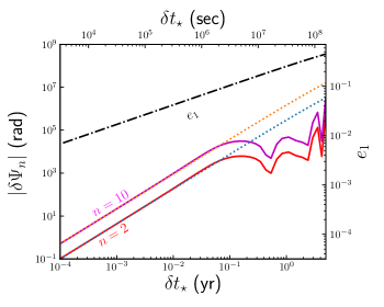
Figure 11: The increase of Fourier phase drift of an example BBH rotating around MBH as a function of time to coalescence $\delta t_{\star}$. Here $M_{\bullet}=10^{6}M_{\odot}$, the BBH is with $m_{A}=m_{B}=10M_{\odot}$, $a_{2}=100{\rm AU}$ and $e_{2}=0.6$, where $a_{2}$ and $e_{2}$ is the SMA and eccentricity of the outer orbit of BBH, respectively. The BBH coalesces with $e_{\rm iso}=5\times 10^{-5}$. The dash-dot line show the evolution of the inner eccentricity of the BBH ($e_{1}$). The dotted lines are prediction from Equation C9; the solid lines are results from Equation C6.

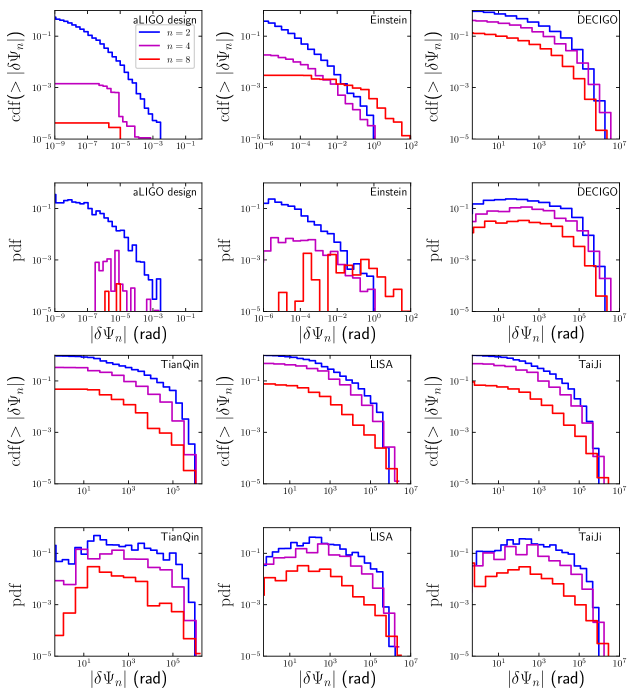
Figure 12: The cdf (top panels) or pdf (bottom panels) of the Doppler drift $\delta\Psi_{n}$ in Fourier phases of the inspiralling or merging BBHs in different observatories (only for samples with $e_{i}<0.4$ and SNR $\rho>8$) in model MP1. Here $n$ is the order of harmonics. Only $\delta\Psi_{n}$ of samples with strain $h_{c,n}$ of the $n$-th harmonic above the sensitivity of the observatory are considered in this plot. The results for other models are similar.

As shown in Section 2.3, there is a fraction of BBHs that can inspiral/merge very close to the MBH (See Table 2). The inner most orbit of BBHs is limited by the tidal radius, thus the periapsis of the outer orbit of BBH should satisfy:

$$r_{p,\rm min} \mathrel{\mathchoice{\lower 4.0pt\vbox{\halign{$\nms\displaystyle\hfil#\hfil$\cr>\crcr\sim\crcr}}}{\lower 4.0pt\vbox{\halign{$\nms\textstyle\hfil#\hfil$\cr>\crcr\sim\crcr}}}{\lower 4.0pt\vbox{\halign{$\nms\scriptstyle\hfil#\hfil$\cr>\crcr\sim\crcr}}}{\lower 4.0pt\vbox{\halign{$\nms\scriptscriptstyle\hfil#\hfil$\cr>\crcr\sim\crcr}}}}a_{1}\left(\frac{3M_{\bullet}}{m_{A}+m_{B}}\right)^{1/3}$$ (10)

$$\mathrel{\mathchoice{\lower 4.0pt\vbox{\halign{$\nms\displaystyle\hfil#\hfil$\cr>\crcr\sim\crcr}}}{\lower 4.0pt\vbox{\halign{$\nms\textstyle\hfil#\hfil$\cr>\crcr\sim\crcr}}}{\lower 4.0pt\vbox{\halign{$\nms\scriptstyle\hfil#\hfil$\cr>\crcr\sim\crcr}}}{\lower 4.0pt\vbox{\halign{$\nms\scriptscriptstyle\hfil#\hfil$\cr>\crcr\sim\crcr}}}} 266r_{\rm SW}\times\frac{a_{1}}{0.1~{}\rm AU}\left(\frac{M_{\bullet}}{10^{6}M_{\odot}}\right)^{-2/3}\left(\frac{m_{A}+m_{B}}{20M_{\odot}}\right)^{-1/3}$$

where $a_{1}$ is the SMA of the inner orbit of BBH. If $a_{1}=0.1\rm AU$, $r_{p,\rm min}$ varies between $10^{3}-10r_{\rm SW}$ for MBHs with masses vary from $10^{5}M_{\odot}$ to $10^{8}M_{\odot}$.

By using the samples obtained in Section 3.2, we can estimate the distributions and the number of inspiralling/merging BBHs with SNR$>8$ and at distance $r<10^{3}r_{\rm SW}$ in different observatories. The results are shown in Figure 8 and  10 and Table 3.

Figure 10 show the pdf of the distance of the inspiralling/merging BBHs to the MBH in different observatories. The distribution of BBHs peaks around $10^{5}r_{\rm SW}$ where $r_{\rm SW}$ is the Schwarzschild radius, almost independent with the observatories. The fraction of BBHs within some given radius $r$ decreases rapidly with $r$. From Figure 10 and Table 3, we can see that the probability of $r<10^{3}r_{\rm SW}$ is about $0.1\%-2\%$. Thus for aLIGO/Virgo(O2), aLIGO(design), or Einstein, in a five years mission, there are about $\sim 1$, $1\sim 10$ and $10-100$ of them can be detected, respectively (See Figure 8). For DECIGO, the expected number can be $10-1000$, however, for LISA/TaiJi, it is very marginally ($\sim 1$). TianQin can not observe such samples as their expected number are smaller than one. We note that the space observatories are more powerful in revealing the relativistic effects of the samples that is very close to the MBH, as their observation time is much longer than those in aLIGO and Einstein.

Due to the existence of a MBH in the vicinity of the inspiralling/merging BBH, the GW radiation will show some unique properties, which is quite different from those BBHs in other environments (e.g., the BBHs in the field regions or globular clusters). For example, if the inspiralling/merging BBHs are sufficiently close to the MBH, they will experience significant accelerations or relativistic effects including gravitational redshift, lensing, and relativistic orbital precession. These effects modify the observed gravitational waveforms in a way very similar to those of the pulsar timing observation, which could cause de-phase of the wave and thus possibly measurable in the current or future GW observatories (e.g., Meiron et al., 2017; Inayoshi et al., 2017). These BBHs provide unique probes for testing relativity in the vicinity of MBHs, and their unique features in waveforms can be used to distinguish the BBHs merging around MBHs in galactic nucleus from those in other environments.

As a first study, here we investigate and discuss only the Doppler drift effects due to the accelerations of the BBHs around a MBH. These effects can be easily analyzed by using some analytical methods if the orbits of the BBHs are near circular. However, it may be more difficult for eccentric BBHs, as their evolution in the Fourier domain is more complex than those of circular ones (Tanay et al., 2016; Yunes et al., 2009; Nishizawa et al., 2016; Moore et al., 2018). For simplicity, here we only estimate the Doppler drift effects of BBHs with entering eccentricity $e_{i}<0.4$, by using the Fourier phase formalism from Yunes et al. (2009) which ignore other PN orders of the orbit (expect the GW orbital decay). The Doppler drift effects for higher eccentric events or including other PN orders will defer to future studies.

According to Figure 9, the eccentricities of BBHs are usually quite low in aLIGO and Einstein observations, with $\mathrel{\mathchoice{\lower 4.0pt\vbox{\halign{$\nms\displaystyle\hfil#\hfil$\cr>\crcr\sim\crcr}}}{\lower 4.0pt\vbox{\halign{$\nms\textstyle\hfil#\hfil$\cr>\crcr\sim\crcr}}}{\lower 4.0pt\vbox{\halign{$\nms\scriptstyle\hfil#\hfil$\cr>\crcr\sim\crcr}}}{\lower 4.0pt\vbox{\halign{$\nms\scriptscriptstyle\hfil#\hfil$\cr>\crcr\sim\crcr}}}}98\%$ of $e_{i}<0.4$, and the fraction of BBHs with $e_{i}<0.4$ is $60\sim 80\%$ in DECIGO/LISA/TianQin/TaiJi band. Our estimation of the Doppler drift should cover a majority of all the detectable events.

Details of the derivation of the Fourier phase drift of BBHs due to its Keplerian motion around MBH can be found in Appendix C. To estimate the phase drift given the order of harmonic $n$ we need to select a time of reference. It is defined as the time at the end of the mission, or the time when the characteristic strain of the BBH $h_{c,n}$ of the $n$-th harmonic moves just below the detection sensitivity. For aLIGO/Einstein and $n=2$, it is usually the time of coalescence. If $h_{c,n}$ of the $n$-th harmonic is below the sensitivity during the whole mission time, we consider that it is not detectable.

In the case when the eccentricity of BBH $e_{1}$ is small and the coalescence time is the time of reference, the phase drift of the $n$-th harmonic can be estimated by Equation C9 (up to orders of $e_{i}^{2}$)

$$| \delta\Psi_{n}|=0.102\times M_{6}^{-1}r_{4}^{-2}f_{1{\rm Hz}}^{-13/3}\mathcal{M}_{14}^{-10/3}\left(\frac{n}{2}\right)^{16/3}\sin I_{2}$$ (11)

$$\times\mathscr{P}(E^{\prime},e_{2},\omega_{2})\left(1-\frac{314}{43}e_{i}^{2}\chi^{-19/9}\right)$$

where $e_{i}$ is the entering eccentricity of the BBH, $\chi=f/f_{i}$ and $f_{i}$ is the GW frequency of the BBH when $e_{1}=e_{i}$, $M_{6}=M_{\bullet}/10^{6}M_{\odot}$, $\mathcal{M}_{14}=\mathcal{M}/14M_{\odot}$, $r_{4}=r/10^{4}{~{}r_{\rm SW}}$ and $f_{1{\rm Hz}}=f/1{\rm~{}Hz}$. $\mathscr{P}\mathrel{\mathchoice{\lower 4.0pt\vbox{\halign{$\nms\displaystyle\hfil#\hfil$\cr<\crcr\sim\crcr}}}{\lower 4.0pt\vbox{\halign{$\nms\textstyle\hfil#\hfil$\cr<\crcr\sim\crcr}}}{\lower 4.0pt\vbox{\halign{$\nms\scriptstyle\hfil#\hfil$\cr<\crcr\sim\crcr}}}{\lower 4.0pt\vbox{\halign{$\nms\scriptscriptstyle\hfil#\hfil$\cr<\crcr\sim\crcr}}}}1$ is a factor determined by the line of sight position of BBH, given by

$$\mathscr{P}=\frac{\sin\omega_{2}(\cos E^{\prime}-e_{2})+(1-e_{2}^{2})^{1/2}\cos\omega_{2}\sin E^{\prime}}{1-e_{2}\cos E^{\prime}}$$ (12)

where $E^{\prime}$ is the eccentric anomaly at the reference position. $e_{2}$, $I_{2}$ and $\omega_{2}$ is the eccentricity, inclination and the argument of periapsis of the outer orbit of the BBH around MBH.

We can see that at a given time, $\delta\Psi_{n}\propto(f/n)^{-13/3}n\propto n$, thus it will be easier to observe phase drift effects in the high order harmonics for eccentric BBHs. However, note that $h_{c,n}$ of the $n$-th harmonic has to be above the noise level of an observatory such that it can measured. An example of the phase drift of a BBH is shown in Figure 11.

The drift of the Fourier phase of a BBH due to acceleration can be observed only if the perturbations on the strain amplitudes are large enough. The signal to noise ratio can be estimated by  (Kocsis et al., 2011)

$$\rho^{2}_{\delta\Psi}=2\sum^{n_{\rm max}}_{n=1}\int^{f_{\rm max}}_{f_{\rm min}}\frac{h_{c,n}^{2}(f)(1-\cos\delta\Psi_{n})}{fS_{n}(f)}\frac{df}{f}$$ (13)

To detect such perturbations in observatories, it is required that at least one of the $n$-th harmonics of $h_{c,n}$ ($n=1,2,\cdots$) is sufficiently above the noise level, and that the corresponding $|\delta\Psi_{n}|$ is also sufficiently larger than unity. For aLIGO, the eccentricities of most BBHs are quite low, thus the most important order is $n=2$. According to Equation 11 we have $f_{1}=10$ and $|\delta\Psi_{2}|\sim 5\times 10^{-4}$ even if $r_{4}\sim 0.1$, thus it is not possible to observe Doppler drift in aLIGO band. Such a small drift is a result of the extremely short time the BBHs spent in aLIGO band (typically in orders of $1-10$ seconds) respect to the orbital time of BBH around MBH ($\mathrel{\mathchoice{\lower 4.0pt\vbox{\halign{$\nms\displaystyle\hfil#\hfil$\cr>\crcr\sim\crcr}}}{\lower 4.0pt\vbox{\halign{$\nms\textstyle\hfil#\hfil$\cr>\crcr\sim\crcr}}}{\lower 4.0pt\vbox{\halign{$\nms\scriptstyle\hfil#\hfil$\cr>\crcr\sim\crcr}}}{\lower 4.0pt\vbox{\halign{$\nms\scriptscriptstyle\hfil#\hfil$\cr>\crcr\sim\crcr}}}}$days if $a_{2}\mathrel{\mathchoice{\lower 4.0pt\vbox{\halign{$\nms\displaystyle\hfil#\hfil$\cr>\crcr\sim\crcr}}}{\lower 4.0pt\vbox{\halign{$\nms\textstyle\hfil#\hfil$\cr>\crcr\sim\crcr}}}{\lower 4.0pt\vbox{\halign{$\nms\scriptstyle\hfil#\hfil$\cr>\crcr\sim\crcr}}}{\lower 4.0pt\vbox{\halign{$\nms\scriptscriptstyle\hfil#\hfil$\cr>\crcr\sim\crcr}}}}10^{3}r_{\rm SW}$). Figure 12 show the distributions of $\delta\Psi_{n}$ for different orders of $n$ for those BBHs with $\rho>8$. We can see that for aLIGO the maximum possible value of $|\delta\Psi_{2}|$ is about $10^{-3}$, and we do not expect to see any Doppler drift effects in aLIGO (See also Figure 8).

For Einstein the lookback time of BBHs coalescence can be about a few hours and the eccentricities of BBHs are slightly higher than aLIGO. It is interesting to see that the large phase drift come from those harmonics of high order (See Figure 12), as for many highly-eccentric BBHs, only high order harmonics of strains appear earlier in Einstein band, instead of the low order ones (See the bottom panels of Figure 4) at a given time. Thus, according to Equation 11 the Doppler drift can be observable if $f_{1}\sim 1$, $r_{4}\sim 0.1$ and $n>2$, however, the probability of $r_{4}\mathrel{\mathchoice{\lower 4.0pt\vbox{\halign{$\nms\displaystyle\hfil#\hfil$\cr<\crcr\sim\crcr}}}{\lower 4.0pt\vbox{\halign{$\nms\textstyle\hfil#\hfil$\cr<\crcr\sim\crcr}}}{\lower 4.0pt\vbox{\halign{$\nms\scriptstyle\hfil#\hfil$\cr<\crcr\sim\crcr}}}{\lower 4.0pt\vbox{\halign{$\nms\scriptscriptstyle\hfil#\hfil$\cr<\crcr\sim\crcr}}}}0.1$ is about $10^{-3}$ as shown in Figure 10. Nevertheless, we find that the expected number of samples with $\rho>8$ and $\rho_{\delta\Psi}>8$ in Einstein telescope can be up to $\sim 10$ (See Figure 8).

For the space observatories, the drift of phase in a $5$-yr’s mission is so large that the approximation given by Equation 11 is no longer valid, and we need to use explicitly the Equation C6 for accurate estimation. As shown in Figure 12, in DECIGO/LISA/TaiJi/TianQin band, the distributions of $\delta\Psi_{n}$ for $n=2$, $n=4$ and $n=8$ all peak around $10-10^{3}$. Most of the BBHs are with phase drift contribute from $n=2$, which is larger than those of higher order ones, such as $n=4$ and $n=8$. This is mainly because we focus on samples with $e_{i}<0.4$, and thus many of the high order harmonics of GW are below the sensitivity level of space observatories (See Top-right panel of Figure 4). The observable numbers of phase drift with $\rho_{\delta\Psi}>8$ and $\rho>8$ can be up to $10^{4}-10^{5}$ for DECIGO, $\sim 30$ for TianQin and $\sim 100$ for LISA/TaiJi, which is about $\sim 30-80\%$ of all detectable samples, see Table 3.

Note that the above estimations are for samples with entering eccentricity $e_{i}<0.4$. Thus, for space telescopes the actual number of samples with detectable Doppler drift should be higher, especially for DECIGO.

6 Gravitational wave backgrounds of BBHs

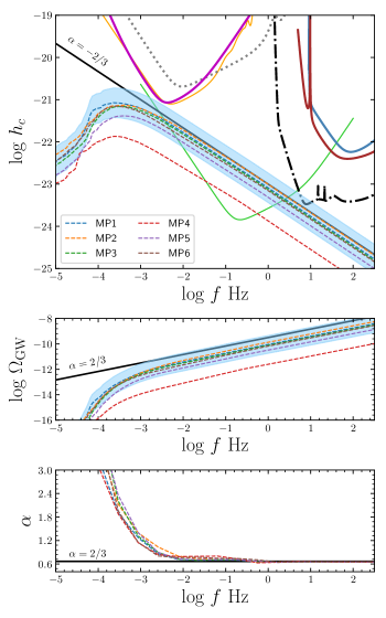
Figure 13: GWB in different models. Top panel: The characteritic strain amplitude of GWB from different models. The shaded region show the uncertainties in model MP1, due to the uncertainties in event rates. The uncertainties is similar for other models and thus not showed here for clarity of the figure. The black solid line show a reference slope of $\alpha=-2/3$; Middle panel: Similar to top panel but for the energy density of GWB from different models. The black solid line show a reference slope of $\alpha=2/3$; Bottom panel: The powerlaw slope of $\Omega_{\rm GW}$ in different models as a function of frequency.

The total number of inspiralling BBHs at any moment can be up to billions (See the estimation at the end of Section 3.2.1). They appear in a GW observatory as a background noise as the majorities of them are weak and slowly evolving BBHs. As many of the BBHs inspiralling/merging around MBH are with high eccentricity, the gravitational wave background (GWB) contributed by these objects are expected different from those of circular inspiralling/merging BBHs (e.g., Zhao & Lu, 2020). Here we investigate the GWB by using the BBH samples obtained from GNC simulations.

The GWB can be estimated by (Phinney, 2001)

$$h_{c,bkg}^{2}(f)=\frac{4G^{5/3}}{3\pi^{1/3}c^{2}f^{4/3}}\iiint de_{0}d\mathcal{M}dz\times$$ (14)

$$\frac{d^{3}N(\mathcal{M},e_{0},z)}{d\mathcal{M}de_{0}dz}\frac{\mathcal{M}^{5/3}}{(1+z)^{1/3}}\sum_{n=1}^{\infty}\left(\frac{2}{n}\right)^{2/3}\frac{g(n,e)}{F(e)}$$

where $g(n,e)$ and $F(e)$ is given by Equation B2 and B3, respectively. $d^{3}N(\mathcal{M},e_{0},z)/d\mathcal{M}de_{0}dz$ is the number distribution function of BBHs. The eccentricity $e$ in the above equation is determined by the following relation for a given value of $e_{0}$, $n$ (the order of harmonics) and $f$:

$$\frac{f}{f_{0}}=\left[\frac{1-e_{0}^{2}}{1-e^{2}}\left(\frac{e}{e_{0}}\right)^{12/19}\left(\frac{1+121e^{2}/304}{1+121e_{0}^{2}/304}\right)^{870/2299}\right]^{-3/2}$$ (15)

where $f_{0}=nF_{\rm orb}$, and $F_{\rm orb}$ is the initial orbital frequency given the initial eccentricity $e_{0}$.

We can obtain individual BBH samples from the GNC rather than its distribution, thus we can use the Monte-Carlo integration to estimate the strain amplitude of the GWB, which is much more simple and straight foward. For more details see Appendix D.

The strain of GWB for different models can be found in Figure 13. We found that the characteristic strain amplitude of GW backgrounds follows well a powerlaw profile of $h_{c,bkg}\propto f^{-2/3}$ when $f>1$mHz, similar to those from circular BBHs (Phinney, 2001). However, the slope changes below $f<1$mHz as the eccentric inspiralling BBHs start to dominate the GWB at those low frequency regions, which is also consistent with those from Zhao & Lu (2020). The energy density of the GWB, i.e., $\Omega_{\rm GW}=2\pi^{2}h_{c,bkg}^{2}(f)f^{2}/(3H_{0}^{2})$, for different models are shown in Figure 13. Similarly, we find that the energy density $\Omega_{\rm GW}\propto f^{2/3}$ if $f\mathrel{\mathchoice{\lower 4.0pt\vbox{\halign{$\nms\displaystyle\hfil#\hfil$\cr>\crcr\sim\crcr}}}{\lower 4.0pt\vbox{\halign{$\nms\textstyle\hfil#\hfil$\cr>\crcr\sim\crcr}}}{\lower 4.0pt\vbox{\halign{$\nms\scriptstyle\hfil#\hfil$\cr>\crcr\sim\crcr}}}{\lower 4.0pt\vbox{\halign{$\nms\scriptscriptstyle\hfil#\hfil$\cr>\crcr\sim\crcr}}}}1$mHz. The power-law slope changes to $\sim 1.2$ at $f\sim 1$mHz and higher if $f<1$mHz. As LISA can put constraints on the GWB above $\Omega_{\rm GW}>10^{-14}$ at $f\sim 1$mHz (See Figure 3 of Abbott et al., 2017a), we expect that LISA/TaiJi/DECIGO can be used to distinguish different merging channels by measuring the profile of GWB.

7 discussion

There are some unique phenomena proposed for BBHs merging around MBH. For example, the b-EMRIs (Chen & Han, 2018), Doppler abbreviation (Torres-Orjuela et al., 2020), relativistic effects (Meiron et al., 2017), lensing effects(D’Orazio & Loeb, 2020; Kocsis, 2013), and etc. To observe these effects, the position of the inspiralling/merging BBHs should be very close to the MBH. We find that there are mainly two factors that affect the closest distance between a BBH and MBH. The first one is the size of the loss cone region of the MBH, which is due to the tidal force of the MBH and it puts a very solid boundary of the BBHs. Thus, almost independent of the initial conditions of the models (expect model MP4, see below), the probability of BBHs merging at distance $r<10^{3}r_{\rm SW}$ is always about $10^{-3}-10^{-2}$. The second factor is the mass of the background objects. If the background object is massive (e.g., $m_{\star}=10M_{\odot}$ in model MP4), the encounters of BBHs with them have a high probability of ionization and they will likely be destroyed before moving into the inner most region.

Comparing models of MP1 and MP2, we find that placing the birth position of BBHs into more inner regions can increase simultaneously the fraction of BBH being merged, tidally disrupted, and ionized (such that BBHs remain integrity is reduced). This will result in a higher merging rate and the predicted total number of samples detectable ($\rho>8$) in different observatories. However, the fraction of samples in the vicinity of MBH are almost unchanged, mainly due to the solid boundary of the loss cone set by the MBH.

Comparing the results of MP3 to other models, we find that if initially the BBHs are born with zero eccentricity, the merging rates, distribution of the merging position of BBHs and other properties of BBHs are not significantly affected. This is mainly because the information of the initial value of the eccentricity will be lost after experiencing large number of multiple dynamical process, including the KL oscillation, encounters with the background objects or with the MBH. The distribution of eccentricities of BBHs in an equilibrium state is then shaped by these dynamical evolution rather than the initial condition of the eccentricities.

Comparing models of MP6 to other models, we find that if the background components are mixed with single black holes ($10M_{\odot}$) and stars ($1M_{\odot}$), the dynamical evolution of BBHs is similar to those assuming background stars with $1M_{\odot}$. This is mainly because the single BHs always contribute a small fraction of the numbers ($\sim 10^{-3}$) and masses ($\sim 10^{-2}$) of the cluster, expect those of the most inner regions. For a Milky way size MBH, the enclosed mass of BHs surpass those of the single stars within radius of about $10^{3}$ AU (Alexander & Hopman, 2009), thus the majorities of the cluster are not affected by the existence of these BHs. The overall effect is a slight increase of the ionization rates of the BHs (from $\sim 1-7\%$ to $5-11\%$).

Assuming that the IMF of stars formed in galactic nuclei follows a top-heavy one, effective mass segregation due to relaxation leads to a mass function that appears to be between the “LIGO_BK” of MP1 and Salpeter-like IMF of MP5. To explore the effects, we run an additional simulation of model that is similar to MP5 but with $\propto m_{A}^{-1.8}$. We find that both the event rates and the predicted number of samples in different observatories are between those predicted from the two above models. This suggests that the two model would provide an upper and lower bound of the predicted numbers of the merging BBHs, respectively.

Here in this work we limit our samples with $z<2$. For higher redshift the structure of the nuclear star cluster around the MBH may be different from those in local universe, thus the results may not be reliable if we expanding to higher redshift. However, Einstein telescope can observe samples with $z>2$, and our predicted numbers of Einstein is only a lower limit of their total sample sizes. The samples from Einstein telescope in the future can help to study the evolution of BBHs in galactic nuclei in high redshift.

8 The planned future updates of the Monte-Carlo code

It is very important to study the hierarchical formation of BBHs and the distinct signatures between the first and multiple generation of BBH mergers (e.g., see a recent review in Gerosa & Fishbach, 2021). It is suggested that GW190521 might come from second-generation mergers due to its large component masses inside the mass gap (Abbott et al., 2020), supporting their dynamical formation hypothesis. In the meanwhile, investigating presented features of EMRIs together with those BBH mergers in galactic nuclei is also important to understand the formation and evolution of MBH in near-by universe (See a review in Amaro-Seoane, 2018).

However, due to some limitations of the current GNC code, we are unable to provide reasonable estimations for these GW events. For example, if the exchange event of a BBH with a background object happens in current GNC code, the simulation stops and thus the following evolution of the BBHs are not calculated and the sample is abandoned for simplicity. Also, the evolution of a BBH stops when it is found merging, and thus the possibility that its merged remnant merging with another BH (i.e., producing the second generation merger) are not included in the simulation. Another limitation is that each components of the cluster is assumed to follow a given power law distribution (e.g. for stars $\propto r^{-7/4}$ or $\propto r^{-1.4}$) and the depletion of background objects due to tidal disruption (for stars) or falling into MBHs (for compact objects) and the exchange between the background objects with BBHs are not included in the simulation. Thus, the results presented in this work are all for first generation BBH mergers. For comprehensive and self-consistent study of GW merging events, including multiple generation of BBH mergers and also the EMRIs in galactic nuclei, we plan to include the following functionalities into GNC in future:

• Evolving multiple species background component. As these background components can be also affected by the tidal disruption of MBH (for stars), or EMRIs (for compact objects), the rejuvenation of them due to the disrupted, ionized or merged BBHs, we can update the profile of background objects according to these events and then obtain a self-consistent steady-state Fokker-Planck solution of the density profiles for the background components.

• Follows the evolution of both the BBHs that have exchanged components with background objects, and the evolution of component being exchanged into background species. For example, a BBH may become a BH-MS binary with the exchange with a background star, and the BH component exchanged become one of the background BH species. If a BBH exchange with those first-generation BBH mergers, a second generation BBH mergers may happen.

• The dynamical evolution of individual background objects, including two-body and resonant relaxations. By including such evolution, we are then able to study the dynamical evolution and the properties (e.g., event rates) of EMRI in galactic nuclei.

• The spinning of the merging BBHs and the GW recoil kick velocity due to the merging of a BBH. The spin distribution of the hierarchical BBH mergers can possible be affected by the dynamically evolution and GW recoil kick may significantly affect the orbital evolution of the BBH mergers, if it is not kicked out from the galactic nuclei. The distribution of spin and also the masses of the BBH mergers provide another dimension in distinguishing different merging channels.

• Stellar evolution, such that the composition of background components and also the compact binaries as a result of stellar evolution of stars (or binary stars) can be estimated self-consistently under different metalicities. In the meanwhile, the stellar evolution of those BH-MS binary can be traced, which may become BBH or other black hole compact binaries in the later stage of the simulation.

• Tidal dissipation of stellar objects. For those BH-MS binary during the Kozai-Lidov oscillation, and those BBHs encountering with a background stars, the tidal dissipation may affect the evolution significantly, and thus tidal dissipation should be added into the code for self-consistency.

• Considering various components of compact objects, such as neutron stars (NS) or white dwarfs (WD) in both the background species and also the compact binaries. Such that we can be able to discuss the evolution and merging of various types of compact binaries, especially BH-NS, BH-WD binaries or NS binaries.

By implementing the above features, GNC will become a more powerful tool to study the complex interplay between various types of compact objects under a number of dynamical effects around MBH. Many of these phenomena can be treated in a self-consistent way, such that we can provide accurate predictions of the hierarchical binary merging events (e.g., distribution of mass, spin, eccentricity, and other unique features) and EMRI events. These predictions can then be useful for distinguishing GW merging sources in galactic nuclei and those in other merging channels.

9 conclusions

Stellar binary black holes (BBHs) merging around the MBH have same unique features, for example, extremely high eccentricities and locating at the very vicinity of the MBH that cause very large accelerations of their motion. We study the properties of these unique features by updated numerical methods of Zhang et al. (2019) (named GNC). We also study the detection of these BBHs in ground or space gravitational wave observatories, including aLIGO/Virgo, Einstein, DECIGO, LISA, TianQin and TaiJi.

We find that $3-40\%$ of all newly formed BBHs will finally merged due to various dynamical effects. A significant fraction of them are merged due to encounters with the background stars ($7\%-90\%$) and KL effects ($6\%-70\%$). The rest of them ($1-25\%$) are merged after one or multiple encounters with the MBH. Some of these events ($40\%-70\%$) can have extremely high eccentricities ($1-e_{1}\mathrel{\mathchoice{\lower 4.0pt\vbox{\halign{$\nms\displaystyle\hfil#\hfil$\cr<\crcr\sim\crcr}}}{\lower 4.0pt\vbox{\halign{$\nms\textstyle\hfil#\hfil$\cr<\crcr\sim\crcr}}}{\lower 4.0pt\vbox{\halign{$\nms\scriptstyle\hfil#\hfil$\cr<\crcr\sim\crcr}}}{\lower 4.0pt\vbox{\halign{$\nms\scriptscriptstyle\hfil#\hfil$\cr<\crcr\sim\crcr}}}}10^{-3}$), or locate very close to the MBH with $r<10^{4}r_{\rm SW}$ (up to $10\%$) when the gravitational wave dominates the inner orbital evolution.

We find that in a five year’s mission, the number of inspiralling/merging BBHs with SNR$>8$ can be up to $\sim 10^{4}$ in aLIGO, $\sim 10^{5}$ in Einstein/DECIGO, $\sim 50$ in TianQin, and $\sim 200$ in LISA/TaiJi band. Some of them can be observed in multiple band observations. For example, there are about $\sim 10$ samples both detectable in LISA/TaiJi/TianQin and aLIGO band with SNR$>8$; Up to $\sim 10^{4}$ samples can be both detectable in DECIGO and aLIGO band with SNR$>8$.

Due to the existence of the central MBH, these BBHs have two unique characteristics:

1. Significant eccentricities. The fraction of high entering eccentricity $e_{i}>0.1$ for different observatories are: aLIGO/Virgo(O2)/aLIGO(design) ($1-3\%$), Einstein ($2-7\%$), DECIGO ($50-70\%$) TianQin ($30-65\%$) and LISA ($30-90\%$). The significant eccentricities of these events provide a possible explanation for the event GW 190521. Due to very high orbital eccentricity, many of the BBHs entering into the aLIGO/Einstein band are not previously detectable in LISA/TaiJi/TianQin band as the strain amplitude become significant only if gravitational wave frequency $>0.1$Hz. Thus, DECIGO become the most ideal obsevatory in probing the rising phases of these extremely high eccentricy GW events.

2. We find that $\sim 0.1\%-2\%$ of the BBHs can merge in distance less than $10^{3}r_{\rm SW}$. These samples have very large acceleration and may also have some significant relativistic effects. We explore the Doppler drift effects in the Fourier phases which can be detectable with SNR$>8$. We find that the number of them with SNR$>8$ are up to $\sim 10^{4}-10^{5}$ in DECIGO, $\sim 30$ in TianQin and $\sim 10^{2}$ in LISA/TaiJi. For Einstein the expected numbers of detection can be up to $\sim 10$.

We find that the gravitational wave background from these highly-eccentric BBH have an energy density follows a powlaw slope of $2/3$ if $f>1$mHz, but deviate to $\mathrel{\mathchoice{\lower 4.0pt\vbox{\halign{$\nms\displaystyle\hfil#\hfil$\cr>\crcr\sim\crcr}}}{\lower 4.0pt\vbox{\halign{$\nms\textstyle\hfil#\hfil$\cr>\crcr\sim\crcr}}}{\lower 4.0pt\vbox{\halign{$\nms\scriptstyle\hfil#\hfil$\cr>\crcr\sim\crcr}}}{\lower 4.0pt\vbox{\halign{$\nms\scriptscriptstyle\hfil#\hfil$\cr>\crcr\sim\crcr}}}}1.2$ at frequency $f<1$mHz. Future space-based telescopes, such as LISA/TaiJi/DECIGO can be able to detect such deviations.

The high eccentricity, the strong accelerations (and also relativistic effects) and a different profile of GWB expected from these sources make them distinguishable from other sources, thus interesting for future GW detection and tests of relativities.

Appendix A Updates to the Numerical Method

The numerical Monte-Carlo framework previously developed in Zhang et al. (2019) have now been updated, with the following improvements:

1. We can now consider both the NR and RR diffuion processes of the BBHs under background objects with multiple species. For the two-body relaxation, such extension can be realized by noticing that the diffusion coefficients of BBHs are obtained by suming up the contributions of all the background particles. Following Rosenbluth et al. (1957); Binney & Tremaine (1987), we can show that if there are a number of $N_{b}$ kinds of background objects with mass $m_{i}$, number density function $n_{i}(r)=n_{i,0}(r/r_{h})^{\alpha_{i}}$, here $i=1,\cdots,N_{b}$, where $n_{i,0}$ is the number density of the $i$-th component at position $r_{h}$, $\alpha_{i}$ is the index of the density profile of the $i$-th component. The diffusion coefficients of BBHs from the $i$-th component are given by $D_{i}^{\rm NR}$, then the total diffusion coefficients of BBHs from all the background stars are given by $D^{\rm NR}=\sum_{i}D_{i}^{\rm NR}$.

   For the RR processes, under the assumpsion that the process is a Gaussian random processes, the contributions of multiple species on RR is approximately represented by a single species with effective mass given by $m_{\rm eff}=\langle m^{2}\rangle(r)/\langle m\rangle(r)$, where the average is calculated at a given position $r$ (Kocsis & Tremaine, 2011), the $\mu_{M}=\sum\mu_{i,M}$, where $\mu_{i,M}$ is the procession due to the $i$-th component.

   We also consider the collision between the BBHs with the multiple species of background objects. The total collision rates are given by summing up the rates of individual background species, i.e., $R_{\rm tot}=\sum R_{i}$, where the rates of BBHs colliding with each species is given by $R_{i}$.

2. We now do not use the soft radius anymore in our explicit $3$-body simulation. Instead, for both the BBH-star encounter and the BBH-MBH encounter we added the PN2.5 term to consider the GW damping effects between any pairs of particles $1$ and $2$. For particle $1$, these terms are given by (Blanchet, 2014)

   $$\vec{a}_{1,{\rm PN25}} =\frac{4}{5c^{5}}\frac{G^{2}m_{1}m_{2}}{r_{12}^{3}}\left[\left(\frac{2Gm_{1}}{r_{12}}-\frac{8Gm_{2}}{r_{12}}-v_{12}^{2}\right)\vec{v}_{12}\right.$$ (A1)

   $$\left.+(\hat{r}_{12}\cdot\vec{v}_{12})\left(\frac{52Gm_{2}}{3r_{12}}-\frac{6Gm_{1}}{r_{12}}+3v_{12}^{2}\right)\hat{r}_{12}\right].$$

   where $\vec{r}_{12}$ and $\vec{v}_{12}$ is the relative position and velocity vector between particle $1$ and $2$, respectively. $\hat{r}_{12}$ and $\hat{v}_{12}$ are the corresponding unit vectors. The accelerations for particle $2$ can be obtained by changing the notion $1\leftrightarrow 2$. $\vec{v}_{12}$ and $\hat{r}_{12}$ change sign by such an operation.

   We find that, by including such radiation, the merging rates of BBHs are increased by $\sim 10\%$ compared to those in Paper I that is without such effect.

   Including the GW damping effect can affect the dynamics of the 3-body encounters between a BBH and a star. For example, BBHs in the soft region can become ‘hard’ after the encounter as the GW can radiative away some excess energy between the BBHs and the incoming star. This will also affect the outcome of the orbital corrections of the outer orbit mentioned below.

3. We added the orbital corrections on the outer orbit of the BBH due to a fly-by event between the BBH and a background object. We perform explicit 3-body simulation for each encounter and we can obtain the change of relative velocity at infinity $\Delta\vec{v}^{\prime}$ in the center of mass frame of the three body before and after the encounter. Denote $\vec{v}_{b}$ as the orbital velocity of the outer orbit of BBH when the encounter happens, and $\Delta\vec{v}_{b}$ as its change due to the encounter. Then simply we have

   $$\Delta\vec{v}_{b}=\frac{m_{3}}{m_{\rm BBH}+m_{3}}\Delta\vec{v}^{\prime}$$ (A2)

   where $m_{3}$ is the mass of the incoming background object.

   Then the change of the orbital energy $\Delta E$ and angular momentum $\Delta\vec{h}$ in the MBH frame can be obtained according to corrections of this velocity, assuming that the the encounter is located at position $|\vec{r}|=a_{2}$ of the orbit. Such a correction introduce additional change in the energy and angular momentum of the outer orbit of a BBH, which is effectively an additional diffusion on the outer orbits of the BBHs, in additional to the two-body and resonant relaxation.

4. Other minor refinements. For example, we refine the criteria of when a BBH is dominated by GW radiation during the phase of KL oscillation. A BBH is considered merging only if $10|\dot{e}^{\rm KL}_{1}|<|\dot{e}^{\rm GW}_{1}|$ and $\delta t-t^{\prime}<50T_{\rm GW}$. If $|\dot{e}^{\rm KL}_{1}|>|\dot{e}^{\rm GW}_{1}|$, we then require $r_{p}<(M_{A}+M_{B})G/c^{2}$, such that it can be merged only if the horizon of each black hole touches with each other.

Appendix B The GW harmonic

For the BBHs with chirp mass $\mathcal{M}=(m_{A}m_{B})^{3/5}m_{\rm BBH}^{-1/5}$, and with none-zero eccentricity $e_{1}$, the energy usually emitted in a broad range of harmonics. The energy emitted per GW frequency at the $n$th harmonic at the rest frame of the source is given by (Eq. 20 of Huerta et al., 2015), (Chen et al., 2017)

$$\frac{dE_{n}}{df_{r}}=\frac{(\pi G)^{2/3}(\mathcal{M})^{5/3}}{3(1+z)^{1/3}f^{1/3}}\left(\frac{2}{n}\right)^{2/3}\frac{g(n,e_{1})}{F(e_{1})}$$ (B1)

where function $g(n,e)$ is given by (Peters & Mathews, 1963)

$$g(n,e_{1}) =\frac{n^{4}}{32}\left\{\left[J_{n-2}(ne_{1})-2eJ_{n-1}(ne_{1})+\frac{2}{n}J_{n}(ne_{1})+2e_{1}J_{n+1}(ne_{1})-J_{n+2}(ne_{1})\right]^{2}\right.$$ (B2)

$$\left.+(1-e_{1}^{2})\left[J_{n-2}(ne_{1})-2J_{n}(ne_{1})+J_{n+2}(ne_{1})\right]^{2}+\frac{4}{3n^{2}}J_{n}(ne_{1})^{2}\right\}$$

where $J_{n}$ are Bessel’s functions and $F(e_{1})$ is given by

$$F(e_{1})=\frac{1+\frac{73}{24}e_{1}^{2}+\frac{37}{96}e_{1}^{4}}{(1-e_{1}^{2})^{7/2}}$$ (B3)

The maximum number of harmonics necessary to a precision of $10^{-3}$ can be estimated as(O’Leary et al., 2009)

$$n_{\rm max}=5\frac{(1+e)^{1/2}}{(1-e)^{3/2}}$$ (B4)

For simplicity here the maximum harmonics we considered is $\min(n_{\rm max},10^{5})$.

The calculation of evolution of BBH ends at the last stable orbit (LSO). For a total mass of $m_{\rm BBH}$, the mean orbital frequency (assuming $e_{1}=0$) at LSO is given by

$$F_{\rm LSO}=\frac{c^{3}}{2\pi m_{\rm BBH}G}\frac{1}{6^{3/2}}$$ (B5)

Appendix C The drift of Fourier phase of BBHs

Denote $t_{\star}$ as the proper time of BBH, $t_{\star,c}$ as the proper time of coalescence and $l_{c}$ as the orbital phase before coalescence. If ignoring all relativistic effects, the time of arrival of the GW emitted from the BBHs to the observer is determined simply by the Reomer delay. Assuming Keplerian motion of BBHs around MBH, the time of arrival is given by

$$t=t_{\star}+\Delta_{R}(t_{\star}),$$ (C1)

where

$$\Delta_{R} =\frac{a_{2}}{c}\sin I_{2}\sin\omega_{2}(\cos E^{\prime}-e_{2})+\frac{a_{2}}{c}(1-e_{2}^{2})^{1/2}\sin I_{2}\cos\omega_{2}\sin E^{\prime},$$ (C2)

$$E^{\prime}-e_{2}\sin E^{\prime}=\frac{2\pi}{P_{2}}(t_{\star}-t_{\star,0}).$$

Here $E^{\prime}$ is the eccentric anomaly, $t_{\star,0}$ is the time of pericenter passage and $P_{2}$ is the orbital period of the outer orbit of BBH. $a_{2}$ and $e_{2}$ is the SMA and eccentricity of the outer orbit of the BBH, respectively. $I_{2}$ is the orbital inclination respect to the sky plane and $\omega_{2}$ is the argument of periapsis of the orbit.

BBHs moving in a constant speed respect to the observer will cause a constant shift in measured chirp mass thus the line of signt velocity can not be reconstructed from observation. However, drift of the observed phase of the GW will be measurable if enough accelerations are presented during a period of observation. Similar to Meiron et al. (2017), we call the BBH moving around an MBH the “source” BBH, and suppose that there is a “reference BBH” that has the same velocity with the source BBH, i.e., $v_{\rm ref}$, at a given reference time $t_{r}$ in the observer’s frame. For aLIGO/Einstein telescope, $t_{r}$ is usually the observed time of coalescence. For spaced-based telescopes, $t_{r}$ is either the time at the end of the mission, or the time when the characteristic strain of the BBH $h_{c}$ moves below the detection sensitivity. Denote $t_{\star}^{\prime}$ and $t^{\prime}$ as the proper time of BBH and time of arrival of the GW of the reference BBH, respectively, then we can define the coordinate of time such that the proper time of both the source and the reference BBH at $t_{r}$ is both given by $t_{\star,r}$. Thus, in the reference BBH, we have

$$t^{\prime}=t_{\star}^{\prime}+\Delta_{R}(t_{\star,r})-\frac{v_{\rm ref}}{c}(t_{\star,r}-t_{\star}^{\prime})=t_{\star}^{\prime}+\Delta_{R}(t_{\star,r})-\frac{v_{\rm ref}}{c}\left[t_{r}-\Delta_{R}(t_{\star,r})-t_{\star}^{\prime}\right]$$ (C3)

Denote $l(t_{\star})$ (or $l(t^{\prime}_{\star})$) as the orbital phase at proper time $t_{\star}$ of the source BBH (or $t^{\prime}_{\star}$ of the reference BBH). For eccentric BBHs, the GW radiation has a broad range of harmonics. The Fourier transform of the GW can be calculated in the stationary phase approximation (Bender, 1999). For a BBH with no relative motion respect to the observer, the Fourier phase of the $n$-th harmonic at frequency $f$ is given by

$$\Psi_{n}(f)=-2\pi ft_{\star}(f)+nl[t_{\star}(f)]$$ (C4)

where $t_{\star}$ is the solution of $ndl(t_{\star})/dt_{\star}=f$. For BBHs with $e<0.4$ the phase is provided by Yunes et al. (2009) (ignoring other PN terms expect GW radiation)

$$\Psi_{n}(f) =nl_{c}-2\pi ft_{\star,c}-\frac{3}{128x}\left(\frac{n}{2}\right)^{8/3}\left[1-\frac{2355}{1462}e_{i}^{2}\chi^{-19/9}+e_{i}^{4}\left(\frac{5222765}{998944}\chi^{-38/9}-\frac{2608555}{444448}\chi^{-19/9}\right)\right.$$ (C5)

$$\left.+e_{i}^{6}\left(-\frac{75356125}{3326976}\chi^{-19/3}-\frac{1326481225}{101334144}\chi^{-19/9}+\frac{17355248095}{455518464}\chi^{-38/9}\right)\right.$$

$$+e_{i}^{8}\left(-\frac{250408403375}{1011400704}\chi^{-19/3}+\frac{4537813337273}{39444627456}\chi^{-76/9}-\frac{6505217202575}{277250217984}\chi^{-19/9}\right.$$

$$\left.\left.+\frac{128274289063885}{830865678336}\chi^{-38/9}\right)+\mathcal{O}(e_{i}^{10})\right]$$

where $x=(\pi\mathcal{M}fG/c^{3})^{5/3}$ and $\chi=f/f_{i}$, $e_{i}$ and $f_{i}$ is the entering eccentricity and frequency of the BBH, respectively; $t_{\star,c}$ is the time of coalescence.

If considering the motion of the source BBH and those of the reference BBH, the Fourier phase difference between the two are given by

$$\delta\Psi_{n}(f) =-2\pi f(t-t^{\prime})-n[l(t_{\star})-l(t_{\star}^{\prime})]$$ (C6)

$$=-2\pi f(t-t^{\prime})+\Psi_{n}(f_{0})-\Psi_{n}(f_{0}^{\prime})+2\pi(f_{0}t_{\star}-f_{0}^{\prime}t_{\star}^{\prime})$$

where

$$f_{0}=n\frac{dl(t_{\star})}{dt_{\star}}=\frac{f}{1+v(t_{\star})/c},~{}~{}f_{0}^{\prime}=n\frac{dl(t_{\star}^{\prime})}{dt_{\star}^{\prime}}=\frac{f}{1+v_{\rm ref}/c}$$ (C7)

If $t_{\star}$ is very close to $t_{\star,r}$, denote $\delta t_{\star}=t_{\star,r}-t_{\star}$, using the fact that

$$\frac{d\Psi_{n}(f_{0})}{df_{0}}=-2\pi t_{\star}$$ (C8)

Then Equation C6 reduce to

$$\delta\Psi_{n}(\delta t_{\star}) \simeq\left(\frac{d\Psi_{n}(f_{0})}{df_{0}}+2\pi t_{\star}\right)(f_{0}-f_{0}^{\prime})-\frac{2\pi f}{2c}a_{\rm ref}\delta t_{\star}^{2}$$ (C9)

$$\simeq-\pi f\frac{a_{\rm ref}}{c}\delta t_{\star}^{2}=-\pi nF_{\rm orb}(t_{\star})\frac{a_{\rm ref}}{c}\delta t_{\star}^{2}$$

where $F_{\rm orb}$ is the orbital frequency of BBH, $a_{\rm ref}$ is the line of sight acceleration at proper time $t_{\star,r}$ (or $t_{r}$ at the observer’s frame), which is given by

$$a_{\rm ref}=-\frac{M_{\bullet}Gc}{r(t_{\star,r})^{3}}\Delta_{R}(t_{\star,r})$$ (C10)

$r(t_{\star})=a_{2}(1-e_{2}\cos E^{\prime})$ is the distance to the MBH at local time $t_{\star}$ of the BBH. Note that $t_{\star,r}$ depends on the order of harmonic $n$ as each harmonic rise above the noise level at different time of observation (for a given GW frequency $f$). If the reference time is the time of coalescence ($t_{\star,r}=t_{c}$), then $\delta t_{\star}$ can be expressed as a function of frequency $f$, by using Equation C8, up to orders of $e^{10}_{i}$:

$$\delta t_{\star} =t_{c}-t_{\star}=\frac{5}{256\pi xf}\left(\frac{n}{2}\right)^{8/3}\left[1-\frac{157}{43}e_{i}^{2}\chi^{-19/9}+e_{i}^{4}\left(\frac{1044553}{56544}\chi^{-38/9}-\frac{521711}{39216}\chi^{-19/9}\right)\right.$$ (C11)

$$\left.+e_{i}^{6}\left(-\frac{15071225}{138624}\chi^{-19/3}-\frac{265296245}{8941248}\chi^{-19/9}+\frac{3471049619}{25784064}\chi^{-38/9}\right)\right.$$

$$+e_{i}^{8}\left(-\frac{50081680675}{42141696}\chi^{-19/3}+\frac{31764693360911}{45513031680}\chi^{-76/9}-\frac{1301043440515}{24463254528}\chi^{-19/9}\right.$$

$$\left.\left.+\frac{25654857812777}{47030132736}\chi^{-38/9}\right)+\mathcal{O}(e_{i}^{10})\right]$$

Note that Equation C5 and C11 are only stable when $e_{i}\mathrel{\mathchoice{\lower 4.0pt\vbox{\halign{$\nms\displaystyle\hfil#\hfil$\cr<\crcr\sim\crcr}}}{\lower 4.0pt\vbox{\halign{$\nms\textstyle\hfil#\hfil$\cr<\crcr\sim\crcr}}}{\lower 4.0pt\vbox{\halign{$\nms\scriptstyle\hfil#\hfil$\cr<\crcr\sim\crcr}}}{\lower 4.0pt\vbox{\halign{$\nms\scriptscriptstyle\hfil#\hfil$\cr<\crcr\sim\crcr}}}}0.4$.

Appendix D Estimating GW backgrounds by Monte-Carlo integration

The multiple integration of Equation LABEL:eq:hcbkg_int can be simply reduced to a Monte-Carlo integration:

$$h_{c,bkg}^{2}(f) \simeq\frac{4G^{5/3}}{3\pi^{1/3}c^{2}f^{4/3}}\frac{R_{0}}{N_{\rm tot}}\sum_{i=1}^{N^{\rm tot}}\frac{\mathcal{M}_{i}^{5/3}}{(1+z_{i})^{4/3}}\sum_{n=1}^{\infty}\left(\frac{2}{n}\right)^{2/3}\frac{g(n,e_{i})}{F(e_{i})}$$ (D1)

where $N_{\rm tot}$ is the size of the MC samples (usually $10^{5}$). $\mathcal{M}_{i}$, $z_{i}$ and $e_{i}$ is the chirp mass, redshift and the eccentricity of the $i-$th Monte-Carlo samples. $R_{0}$ is the total merging rate given by

$$R_{0} =\iiint\frac{dN(\mathcal{M},e_{0},z)}{dzde_{0}d\mathcal{M}}dzde_{0}d\mathcal{M}$$ (D2)

$$=\iiiint\frac{dN(\mathcal{M},e_{0},z|M_{\bullet})}{dt_{r}de_{0}d\mathcal{M}}\frac{dt_{r}}{dz}n(M_{\bullet},z)dzde_{0}d\mathcal{M}dM_{\bullet}$$

$$=\iint\frac{R(M_{\bullet})n(M_{\bullet},z)}{(1+z)H_{0}E(z)}dM_{\bullet}dz$$

where $E(z)=[\Omega_{M}(1+z)^{3}+\Omega_{\Lambda}]^{1/2}$, $R(M_{\bullet})$ is the merging rate in the local universe for galaxies with a given MBH mass (Equation 1), $t_{r}$ is local time of BBH, $n(M_{\bullet},z)$ is the number distribution function of MBH given by Aversa et al. (2015). The integration is over all redshift and MBH mass ranges.

According to Chen et al. (2017), this summation can be further reduced to

$$h_{c,bkg}^{2}(f)\simeq \frac{R_{0}}{N_{\rm tot}}\sum_{i=1}^{N^{\rm tot}}\left(\frac{\mathcal{M}_{i}}{\mathcal{M}_{0}}\right)^{5/3}\left(\frac{1+z_{i}}{1+z_{0}}\right)^{-1/3}$$ (D3)

$$\times h_{c,0}^{2}\left(\left.f\frac{f_{p,0}}{f_{p,t}}\right|e_{0},f_{0}\right)\left(\frac{f_{p,t}}{f_{p,0}}\right)^{-4/3}$$

where $\mathcal{M}_{0}=4.16\times 10^{8}M_{\odot}$, $z_{0}=0.02$. $h_{c,0}^{2}(f|e_{0},f_{0})$ is given by Chen et al. (2017) in unit of Mpc^-3, and $f_{p,0}$ is given by the following equation when $f=0.1$nHz and $e=0.9$:

$$\frac{f_{p}}{f}=\frac{1293}{181}\left[\frac{e^{12/19}}{1-e^{2}}(1+\frac{121e^{2}}{304})^{870/2299}\right]^{3/2},$$ (D4)

$f_{p,t}$ is given by the above equation when $f=f_{0}$ and $e=e_{0}$.

To generate Monte-Carlo samples, we take the following steps:

1. Draw a total number of $N_{\rm tot}=10^{5}$ random pairs of $M_{\bullet},z$ following the two-dimensional distribution:

   $$P(M_{\bullet},z)\propto\frac{R(M_{\bullet})n(M_{\bullet},z)}{(1+z)H_{0}E(z)}$$ (D5)

2. For the $i$-th mass and redshift from above (deonted by $M_{\bullet,i}$ and $z_{i}$, respectively), get the samples from each model that is with the mass of MBH closest to $M_{\bullet,i}$ (one of the four GNC runs with $M_{\bullet}=10^{5}M_{\odot},10^{6}M_{\odot},10^{7}M_{\odot}$ and $10^{8}M_{\odot}$). Randomly select one of the sample and get its corresponding value of $\mathcal{M}_{i}$ and $e_{0,i}$.

3. Calculate the GWB according to Equation LABEL:eq:hcbkg_monte_carlo given the $\mathcal{M}_{i}$, $e_{0,i},z_{i}$, $i=1,\cdots,N_{\rm tot}$ of the MC samples for each value of frequency $f$.

References

- Abbott et al. (2016a) Abbott, B. P., Abbott, R., Abbott, T. D., et al. 2016a, Physical Review Letters, 116, 061102
- Abbott et al. (2016b) Abbott, B. P., Abbott, R., Abbott, T. D., et al. 2016b, ApJ, 833, L1
- Abbott et al. (2016c) Abbott, B. P., Abbott, R., Abbott, T. D., et al. 2016c, Physical Review Letters, 116, 241103
- Abbott et al. (2016d) Abbott, B. P., Abbott, R., Abbott, T. D., et al. 2016d, Physical Review X, 6, 041015
- Abbott et al. (2016e) Abbott, B. P., Abbott, R., Abbott, T. D., et al. 2016e, Phys. Rev. D, 93, 122003. doi:10.1103/PhysRevD.93.122003
- Abbott et al. (2017a) Abbott, B. P., Abbott, R., Abbott, T. D., et al. 2017a, Physical Review Letters, 118, 221101
- Abbott et al. (2017b) Abbott, B. P., Abbott, R., Abbott, T. D., et al. 2017b, ApJ, 851, L35
- Abbott et al. (2017c) Abbott, B. P., Abbott, R., Abbott, T. D., et al. 2017c, Physical Review Letters, 119, 141101
- Abbott et al. (2017d) Abbott, B. P., Abbott, R., Abbott, T. D., et al. 2017d, ApJ, 848, L12
- Abbott et al. (2019a) Abbott, B. P., Abbott, R., Abbott, T. D., et al. 2019, Physical Review X, 9, 031040. doi:10.1103/PhysRevX.9.031040
- Abbott et al. (2019b) Abbott, B. P., Abbott, R., Abbott, T. D., et al. 2019, ApJ, 882, L24
- Abbott et al. (2020a) Abbott, R., Abbott, T. D., Abraham, S., et al. 2020, Phys. Rev. Lett., 125, 101102. doi:10.1103/PhysRevLett.125.101102
- Abbott et al. (2020) Abbott, R., Abbott, T. D., Abraham, S., et al. 2020, ApJ, 900, L13. doi:10.3847/2041-8213/aba493
- Abbott et al. (2021) Abbott, R., Abbott, T. D., Abraham, S., et al. 2021, ApJ, 913, L7. doi:10.3847/2041-8213/abe949
- Abbott et al. (2021) Abbott, R., Abbott, T. D., Abraham, S., et al. 2021, Physical Review X, 11, 021053. doi:10.1103/PhysRevX.11.021053
- Alexander (2005) Alexander, T. 2005, Phys. Rep., 419, 65
- Alexander & Hopman (2009) Alexander, T., & Hopman, C. 2009, ApJ, 697, 1861
- Arca Sedda (2020) Arca Sedda, M. 2020, ApJ, 891, 47
- Arca Sedda et al. (2019) Arca Sedda, M., Berry, C. P. L., Jani, K., et al. 2019, arXiv:1908.11375
- Amaro-Seoane et al. (2017) Amaro-Seoane, P., Audley, H., Babak, S., et al. 2017, arXiv:1702.00786
- Amaro-Seoane (2018) Amaro-Seoane, P. 2018, Living Reviews in Relativity, 21, 4. doi:10.1007/s41114-018-0013-8
- Antonini & Perets (2012) Antonini, F., & Perets, H. B. 2012, ApJ, 757, 27
- Antonini & Rasio (2016) Antonini, F., & Rasio, F. A. 2016, ApJ, 831, 187
- Aversa et al. (2015) Aversa, R., Lapi, A., de Zotti, G., Shankar, F., & Danese, L. 2015, ApJ, 810, 74
- Bahcall & Wolf (1976) Bahcall, J. N., & Wolf, R. A. 1976, ApJ, 209, 214
- Barack & Cutler (2004) Barack, L., & Cutler, C. 2004, Phys. Rev. D, 70, 122002
- Barsotti et al. (2012) Barsotti L, Fritschel P (2012) Early aLIGO configurations: example scenarios toward design sensitivity. Technical report LIGO-T1200307-v4, LIGO, Pasadena, CA. https://dcc.ligo.org/LIGO-T1200307/public
- Barsotti et al. (2018) L. Barsotti, S. Gras, M.Evans, & P. Fritschel, 2018, LIGO document LIGO-T1800044-v5, https://dcc.ligo.org/LIGO-T1800044/public
- Bartos et al. (2017) Bartos, I., Kocsis, B., Haiman, Z., & Márka, S. 2017, ApJ, 835, 165
- Belczynski et al. (2004) Belczynski, K., Sadowski, A., & Rasio, F. A. 2004, ApJ, 611, 1068
- Belczynski et al. (2016) Belczynski, K., Holz, D. E., Bulik, T., & O’Shaughnessy, R. 2016, Nature, 534, 512
- Bender (1999) Bender, C. M. 1999, Advanced Mathematical Methods for Scientists and Engineers I. Asymptotic Methods and Perturbation Theory Volume package: Bender,C.M.;Orszag,S.A.: Adv.Math.Methods Scientists,Eng.. Bender, Carl M., Orszag, Steven A., pp. 593. ISBN 0-387-98931-5. Springer-Verlag Berlin Heidelberg 1999, 593
- Binney & Tremaine (1987) Binney, J., & Tremaine, S. Galactic Dynamics, 1987, Princeton, NJ, Princeton University Press, 1987, 747 p.
- Blanchet (2014) Blanchet, L. 2014, Living Reviews in Relativity, 17, 2
- Bonvin et al. (2017) Bonvin, C., Caprini, C., Sturani, R., et al. 2017, Phys. Rev. D, 95, 044029
- Breivik et al. (2016) Breivik, K., Rodriguez, C., Larson S. et al. 2016 ApJ, 830, 18
- Campbell & Matzner (1973) Campbell, G. A. & Matzner, R. A. 1973, Journal of Mathematical Physics, 14, 1. doi:10.1063/1.1666159
- Chen & Han (2018) Chen, X., & Han, W.-B. 2018, Communications Physics, 1, 53
- Chen et al. (2017) Chen, S., Sesana, A., & Del Pozzo, W. 2017, MNRAS, 470, 1738
- Chen & Amaro-Seoane (2017) Chen, X. & Amaro-Seoane, P. 2017, ApJ, 842, L2. doi:10.3847/2041-8213/aa74ce
- Dominik et al. (2015) Dominik, M., Berti, E., O’Shaughnessy, R., et al. 2015, ApJ, 806, 263
- D’Orazio & Samsing (2018) D’Orazio, D. J., & Samsing, J. 2018, MNRAS, 481, 4775
- D’Orazio & Loeb (2020) D’Orazio, D. J. & Loeb, A. 2020, Phys. Rev. D, 101, 083031. doi:10.1103/PhysRevD.101.083031
- Fang et al. (2019) Fang, Y., Chen, X., & Huang, Q.-G. 2019, ApJ, 887, 210. doi:10.3847/1538-4357/ab510e
- Finn & Thorne (2000) Finn, L. S., & Thorne, K. S. 2000, Phys. Rev. D, 62, 124021
- Fragione et al. (2019) Fragione, G., Grishin, E., Leigh, N. W. C., et al. 2019, MNRAS, 488, 47
- Gayathri et al. (2020) Gayathri, V., Healy, J., Lange, J., et al. 2020, arXiv:2009.05461
- Gerosa & Fishbach (2021) Gerosa, D. & Fishbach, M. 2021, Nature Astronomy, 5, 749. doi:10.1038/s41550-021-01398-w
- Gondán et al. (2018) Gondán, L., Kocsis, B., Raffai, P., et al. 2018, ApJ, 860, 5. doi:10.3847/1538-4357/aabfee
- Gondán & Kocsis (2020) Gondán, L. & Kocsis, B. 2020, arXiv:2011.02507
- Hamers et al. (2018) Hamers, A. S., Bar-Or, B., Petrovich, C., & Antonini, F. 2018, ApJ, 865, 2
- Hild et al. (2011) Hild, S., Abernathy, M., Acernese, F., et al. 2011, Classical and Quantum Gravity, 28, 094013. doi:10.1088/0264-9381/28/9/094013
- Hinderer & Babak (2017) Hinderer, T., & Babak, S. 2017, Physical Review D, 96, 104048
- Hoang et al. (2018) Hoang, B.-M., Naoz, S., Kocsis, B., Rasio, F. A., & Dosopoulou, F. 2018, ApJ, 856, 140
- Hoang et al. (2019) Hoang, B.-M., Naoz, S., Kocsis, B., et al. 2019, AAS Division on Dynamical Astronomy meeting #50, id. 202.03. Bulletin of the American Astronomical Society, Vol. 51, No. 5
- Hong & Lee (2015) Hong, J. & Lee, H. M. 2015, MNRAS, 448, 754. doi:10.1093/mnras/stv035
- Huerta et al. (2015) Huerta, E. A., McWilliams, S. T., Gair, J. R., et al. 2015, Phys. Rev. D, 92, 063010
- Inayoshi et al. (2017) Inayoshi, K., Tamanini, N., Caprini, C., et al. 2017, Phys. Rev. D, 96, 063014
- Inayoshi et al. (2017) Inayoshi, K., Hirai, R., Kinugawa, T., et al. 2017, MNRAS, 468, 5020
- Kawamura et al. (2006) Kawamura, S., Nakamura, T., Ando, M., et al. 2006, Classical and Quantum Gravity, 23, S125. doi:10.1088/0264-9381/23/8/S17
- Kawamura et al. (2021) Kawamura, S., Ando, M., Seto, N., et al. 2021, Progress of Theoretical and Experimental Physics, 2021, 05A105. doi:10.1093/ptep/ptab019
- Kocsis & Tremaine (2011) Kocsis, B. & Tremaine, S. 2011, MNRAS, 412, 187. doi:10.1111/j.1365-2966.2010.17897.x
- Kocsis et al. (2011) Kocsis, B., Yunes, N., & Loeb, A. 2011, Phys. Rev. D, 84, 024032
- Kocsis (2013) Kocsis, B. 2013, ApJ, 763, 122. doi:10.1088/0004-637X/763/2/122
- Kozai (1962) Kozai, Y. 1962, AJ, 67, 591
- Kyutoku & Seto (2016) Kyutoku, K., & Seto, N. 2016, MNRAS, 462, 2177
- Lawrence (1973) Lawrence, J. K. 1973, Phys. Rev. D, 7, 2275. doi:10.1103/PhysRevD.7.2275
- Liu & Bromm (2020) Liu, B. & Bromm, V. 2020, arXiv:2009.11447
- Liu et al. (2020a) Liu, C., Shao, L., Zhao, J., & Gao, Y. 2020a, MNRAS, 496, 182
- Liu et al. (2020b) Liu, X., Cao, Z., Shao, L. 2020b, Phys. Rev. D, 101, 044049
- Luo et al. (2016) Luo, J., Chen, L.-S., Duan, H.-Z., et al. 2016, Classical and Quantum Gravity, 33, 035010
- Mandel et al. (2018) Mandel, I., Sesana, A., & Vecchio, A. 2018, Class. Quantum Grav., 35, 054004
- Meiron et al. (2017) Meiron, Y., Kocsis, B., & Loeb, A. 2017, ApJ, 834, 200
- McKernan et al. (2018) McKernan, B., Ford, K. E. S., Bellovary, J., et al. 2018, ApJ, 866, 66. doi:10.3847/1538-4357/aadae5
- Moore et al. (2018) Moore, B., Robson, T., Loutrel, N., et al. 2018, Classical and Quantum Gravity, 35, 235006
- Nishizawa et al. (2016) Nishizawa, A., Berti, E., Klein, A., et al. 2016, Phys. Rev. D, 94, 064020
- O’Leary et al. (2009) O’Leary, R. M., Kocsis, B., & Loeb, A. 2009, MNRAS, 395, 2127
- Peters & Mathews (1963) Peters, P. C., & Mathews, J. 1963, Physical Review, 131, 435
- Petrovich & Antonini (2017) Petrovich, C., & Antonini, F. 2017, ApJ, 846, 146
- Pfuhl et al. (2014) Pfuhl, O., Alexander, T., Gillessen, S., et al. 2014, ApJ, 782, 101. doi:10.1088/0004-637X/782/2/101
- Phinney (2001) Phinney, E. S. 2001, astro-ph/0108028
- Planck Collaboration et al. (2014) Planck Collaboration, Ade, P. A. R., Aghanim, N., et al. 2014, A&A, 571, A16. doi:10.1051/0004-6361/201321591
- Randall & Xianyu (2019) Randall, L. & Xianyu, Z.-Z. 2019, arXiv:1902.08604
- Randall et al (2021) Randall, L., Shelest A. and Xianyu Z. Z., arXiv:2103.16030
- Rauch & Tremaine (1996) Rauch, K. P., & Tremaine, S. 1996, NewA, 1, 149
- Robson et al. (2019) Robson, T., Cornish, N. J., & Liu, C. 2019, Classical and Quantum Gravity, 36, 105011
- Rodriguez et al. (2016a) Rodriguez, C. L., Haster, C.-J., Chatterjee, S., Kalogera, V., & Rasio, F. A. 2016, ApJ, 824, L8
- Rodriguez et al. (2016b) Rodriguez, C. L., Chatterjee, S., & Rasio, F. A. 2016, Phys. Rev. D, 93, 084029
- Rodriguez et al. (2015) Rodriguez, C. L., Morscher, M., Pattabiraman, B., et al. 2015, Physical Review Letters, 115, 051101
- Romero-Shaw et al. (2020) Romero-Shaw, I., Lasky, P. D., Thrane, E., et al. 2020, ApJ, 903, L5. doi:10.3847/2041-8213/abbe26
- Rosenbluth et al. (1957) Rosenbluth, M. N., MacDonald, W. M., & Judd, D. L. 1957, Physical Review, 107, 1. doi:10.1103/PhysRev.107.1
- Ruan et al. (2020) Ruan, W.-H., Guo, Z.-K., Cai, R.-G., et al. 2020, International Journal of Modern Physics A, 35, 2050075. doi:10.1142/S0217751X2050075X
- Shapiro & Marchant (1978) Shapiro, S. L., & Marchant, A. B. 1978, ApJ, 225, 603
- Sesana et al. (2005) Sesana, A., Haardt, F., Madau, P., et al. 2005, ApJ, 623, 23
- Seto (2016) Seto, N. 2016, MNRAS, 460, L1
- Stone et al. (2017) Stone, N. C., Metzger, B. D., & Haiman, Z. 2017, MNRAS, 464, 946
- Tagawa et al. (2020) Tagawa, H., Haiman, Z., & Kocsis, B. 2020, ApJ, 898, 25. doi:10.3847/1538-4357/ab9b8c
- Tanay et al. (2016) Tanay, S., Haney, M., & Gopakumar, A. 2016, Phys. Rev. D, 93, 064031
- Trani et al. (2019) Trani, A. A., Spera, M., Leigh, N. W. C., et al. 2019, ApJ, 885, 135
- Torres-Orjuela et al. (2020) Torres-Orjuela, A., Chen, X., & Amaro-Seoane, P. 2020, Phys. Rev. D, 101, 083028
- Wang et al. (2019) Wang, H.-T., Jiang, Z., Sesana, A., et al. 2019, Phys. Rev. D, 100, 043003. doi:10.1103/PhysRevD.100.043003
- Wen (2003) Wen, L. 2003, ApJ, 598, 419
- Wong et al. (2019) Wong, K. W. K., Baibhav, V., & Berti, E. 2019, MNRAS, 488, 5665
- Yagi & Seto (2011) Yagi, K. & Seto, N. 2011, Phys. Rev. D, 83, 044011. doi:10.1103/PhysRevD.83.044011
- Yunes et al. (2009) Yunes, N., Arun, K. G., Berti, E., et al. 2009, Phys. Rev. D, 80, 084001
- Zhang et al. (2019) Zhang, F., Shao, L., & Zhu, W. 2019, ApJ, 877, 87
- Zhao & Lu (2020) Zhao, Y. & Lu, Y. 2020, MNRAS, 500, 1421. doi:10.1093/mnras/staa2707