Reinforcement Learning for Classical Planning:
Viewing Heuristics as Dense Reward Generators

Abstract

Recent advances in reinforcement learning (RL) have led to a growing interest in applying RL to classical planning domains or applying classical planning methods to some complex RL domains. However, the long-horizon goal-based problems found in classical planning lead to sparse rewards for RL, making direct application inefficient. In this paper, we propose to leverage domain-independent heuristic functions commonly used in the classical planning literature to improve the sample efficiency of RL. These classical heuristics act as dense reward generators to alleviate the sparse-rewards issue and enable our RL agent to learn domain-specific value functions as residuals on these heuristics, making learning easier. Correct application of this technique requires consolidating the discounted metric used in RL and the non-discounted metric used in heuristics. We implement the value functions using Neural Logic Machines, a neural network architecture designed for grounded first-order logic inputs. We demonstrate on several classical planning domains that using classical heuristics for RL allows for good sample efficiency compared to sparse-reward RL. We further show that our learned value functions generalize to novel problem instances in the same domain.

1 Introduction

Deep reinforcement learning (RL) approaches have several strengths over conventional approaches to decision making problems, including compatibility with complex and unstructured observations, little dependency on hand-crafted models, and some robustness to stochastic environments. However, they are notorious for their poor sample complexity; e.g., it may require $10^{10}$ environment interactions to successfully learn a policy for Montezuma’s Revenge (Badia et al. 2020). This sample inefficiency prevents their applications in environments where such an exhaustive set of interactions is physically or financially infeasible. The issue is amplified in domains with sparse rewards and long horizons, where the reward signals for success are difficult to obtain through random interactions with the environment.

In contrast, research in AI Planning and classical planning has been primarily driven by the identification of tractable fragments of originally PSPACE-complete planning problems (Bylander 1994), and the use of the cost of the tractable relaxed problem as domain-independent heuristic guidance for searching through the state space of the original problem. Contrary to RL approaches, classical planning has focused on long-horizon problems with solutions well over 1000 steps long (Jonsson 2007; Asai and Fukunaga 2015). Moreover, classical planning problems inherently have sparse rewards — the objective of classical planning is to produce a sequence of actions that achieves a goal. However, although domain-independence is a welcome advantage, domain-independent methods can be vastly outperformed by carefully engineered domain-specific methods such as a specialized solver for Sokoban (Junghanns and Schaeffer 2000) due to the no-free-lunch theorem for search problems (Wolpert, Macready et al. 1995). Developing such domain-specific heuristics can require intensive engineering effort, with payoff only in that single domain. We are thus interested in developing domain-independent methods for learning domain-specific heuristics.

In this paper, we draw on the strengths of reinforcement learning and classical planning to propose an RL framework for learning to solve STRIPS planning problems. We propose to leverage classical heuristics, derivable automatically from the STRIPS model, to accelerate RL agents to learn a domain-specific neural network value function. The value function, in turn, improves over existing heuristics and accelerates search algorithms at evaluation time.

To operationalize this idea, we use potential-based reward shaping (Ng, Harada, and Russell 1999), a well-known RL technique with guaranteed theoretical properties. A key insight in our approach is to see classical heuristic functions as providing dense rewards that greatly accelerate the learning process in three ways. First, they allow for efficient, informative exploration by initializing a good baseline reactive agent that quickly reaches a goal in each episode during training. Second, instead of learning the value function directly, we learn a residual on the heuristic value, making learning easier. Third, the learning agent receives a reward by reducing the estimated cost-to-go (heuristic value). This effectively mitigates the issue of sparse rewards by allowing the agent to receive positive rewards more frequently.

We implement our neural network value functions as Neural Logic Machines (Dong et al. 2019, NLM), a recently proposed neural network architecture that can directly process first-order logic (FOL) inputs, as are used in classical planning problems. NLM takes a dataset expressed in grounded FOL representations and learns a set of (continuous relaxations of) lifted Horn rules. The main advantage of NLMs is that they structurally generalize across different numbers of terms, corresponding to objects in a STRIPS encoding. Therefore, we find that our learned value functions are able to generalize effectively to problem instances of arbitrary sizes in the same domain.

We provide experimental results that validate the effectiveness of the proposed approach in 8 domains from past IPC (International Planning Competition) benchmarks, providing detailed considerations on the reproducibility of the experiments. We find that our reward shaping approach achieves good sample efficiency compared to sparse-reward RL, and that the use of NLMs allows for generalization to novel problem instances. For example, our system learns from blocksworld instances with 2-6 objects, and the result enhances the performance of solving instances with up to 50 objects.

2 Background

We denote a multi-dimensional array in bold. ${\bm{a}};{\bm{b}}$ denotes a concatenation of tensors ${\bm{a}}$ and ${\bm{b}}$ in the last axis. Functions (e.g., $\log,\exp$) are applied to arrays element-wise.

2.1 Classical Planning

We consider planning problems in the STRIPS subset of PDDL (Fikes and Nilsson 1972), which for simplicity we refer to as lifted STRIPS. We denote such a planning problem as a 5-tuple ${\left<O,P,A,I,G\right>}$. $O$ is a set of objects, $P$ is a set of predicates, and $A$ is a set of actions. We denote the arity of predicates $p\in P$ and action $a\in A$ as $\text{\#}{}p$ and $\text{\#}{}a$, and their parameters as, e.g., $X=(x_{1},\cdots,x_{\text{\#}{}a})$. We denote the set of predicates and actions instantiated on $O$ as $P(O)$ and $A(O)$, respectively, which is a union of Cartesian products of predicates/actions and their arguments, i.e., they represent the set of all ground propositions and actions. A state $s\subseteq P(O)$ is a set of propositions that are true in that state. An action is a 4-tuple ${\left<\textsc{pre}(a),\textsc{add}(a),\textsc{del}(a),\textsc{cost}(a)\right>}$, where $\textsc{pre}(a),\textsc{add}(a),\textsc{del}(a)\in P(X)$ are preconditions, add-effects, and delete-effects, and $\textsc{cost}(a)\in\mathbb{R}$ is a cost of taking the action $a$. In this paper, we primarily assume a unit-cost domain where $\textsc{cost}(a)=1$ for all $a$. Given a current state $s$, a ground action $a_{\dagger}\in A(O)$ is applicable when $\textsc{pre}(a_{\dagger})\subseteq s$, and applying an action $a_{\dagger}$ to $s$ yields a successor state $a_{\dagger}(s)=(s\setminus\textsc{del}(a_{\dagger}))\cup\textsc{add}(a_{\dagger})$. Finally, $I,G\subseteq P(O)$ are the initial state and a goal condition, respectively. The task of classical planning is to find a plan $(a_{\dagger}^{1},\cdots,a_{\dagger}^{n})$ which satisfies $a_{\dagger}^{n}\circ\cdots\circ a_{\dagger}^{1}(I)\supseteq G$ and every action $a_{\dagger}^{i}$ satisfies its preconditions at the time of using it. The machine representation of a state $s$ and the goal condition $G$ is a bitvector of size $|P(O)|=\sum_{p\in P}O^{\text{\#}{}p}$, i.e., the $i$-th value of the vector is 1 when the corresponding $i$-th proposition is in $s$, or $G$.

2.2 Markov Decision Processes

In general, RL methods address domains modeled as a discounted Markov decision processes (MDP), $\mathcal{M}={\left<\mathcal{S},\mathcal{A},T,r,q_{0},\gamma\right>}$ where $\mathcal{S}$ is a set of states, $\mathcal{A}$ is a set of actions, $T(s,a,s^{\prime}):\mathcal{S}\times\mathcal{A}\times\mathcal{S}\rightarrow[0,1]$ encodes the probability $\Pr(s^{\prime}|s,a)$ of transitioning from a state $s$ to a successor state $s^{\prime}$ by an action $a$, $r(s,a,s^{\prime}):\mathcal{S}\times\mathcal{A}\times\mathcal{S}\rightarrow\mathbb{R}$ is a reward function, $q_{0}$ is a probability distribution over initial states, and $0\leq\gamma<1$ is a discount factor. In this paper, we restrict our attention to deterministic models because PDDL domains are deterministic, and we have a deterministic mapping $T^{\prime}:\mathcal{S}\times\mathcal{A}\rightarrow\mathcal{S}$. Given a policy $\pi:\mathcal{S}\times\mathcal{A}\rightarrow[0,1]$ representing a probability $\Pr(a|s)$ of performing an action $a$ in a state $s$, we define a sequence of random variables ${\left\{S_{t}\right\}}^{\infty}_{t=0}$, ${\left\{A_{t}\right\}}^{\infty}_{t=0}$ and ${\left\{R_{t}\right\}}^{\infty}_{t=0}$, representing states, actions and rewards over time $t$.

Our goal is to find a policy maximizing its long term discounted cumulative rewards, formally defined as a value function $V_{\gamma,\pi}(s)=\mathbb{E}_{A_{t}\sim\pi(S_{t},\cdot)}\left[\sum_{t=0}^{\infty}\gamma^{t}R_{t}\mid S_{0}=s\right].$ We also define an action-value function to be the value of executing a given action and subsequently following some policy $\pi$, i.e., $Q_{\gamma,\pi}(s,a)=\mathbb{E}_{S_{1}\sim T(s,a,\cdot)}\left[R_{0}+\gamma V_{\gamma,\pi}(S_{1})\mid S_{0}=s,A_{0}=a\right].$ An optimal policy $\pi^{*}$ is a policy that achieves the optimal value function $V^{*}_{\gamma}=V_{\gamma,\pi^{*}}$ that satisfies $V^{*}_{\gamma}(s)\geq V_{\gamma,\pi}(s)$ for all states and policies. $V^{*}_{\gamma}$ satisfies Bellman’s equation:

$$V^{*}_{\gamma}(s) =\max_{a\in\mathcal{A}}Q^{*}_{\gamma}(s,a)\;\;\;\forall s\in\mathcal{S},$$ (1)

where $Q^{*}_{\gamma}=Q_{\gamma,\pi^{*}}$ is referred to as the optimal action-value function. We may omit $\pi$ in $V_{\gamma,\pi}$, $Q_{\gamma,\pi}$ for clarity.

Finally, we can define a policy by mapping action-values in each state to a probability distribution over actions. For example, given an action-value function, $Q$, we can define a policy $\pi(s,a)=\textsc{softmax}(Q(s,a)/\tau)$, where $\tau>0$ is a temperature that controls the greediness of the policy. It returns a greedy policy $\operatorname*{arg\,max}_{a}Q(s,a)$ when $\tau\rightarrow 0$; and approaches a uniform policy when $\tau\rightarrow\infty$.

2.3 Formulating Classical Planning as an MDP

There are two typical ways to formulate a classical planning problem as an MDP. In one strategy, given a transition $(s,a,s^{\prime})$, one may assign a reward of 1 when $s^{\prime}\in G$, and 0 otherwise (Rivlin, Hazan, and Karpas 2019). In another strategy, one may assign a reward of 0 when $s\in G$, and $-1$ otherwise (or, more generally $-\textsc{cost}(a)$ in a non-unit-cost domain). In this paper we use the second, negative-reward model because it tends to induce more effective exploration in RL due to optimistic initial values (Sutton and Barto 2018). Both cases are considered sparse reward problems because there is no information about whether one action sequence is better than another until a goal state is reached.

3 Bridging Deep RL and AI Planning

We consider a multitask learning setting with a training time and a test time (Fern, Khardon, and Tadepalli 2011). During training, classical planning problems from a single domain are available. At test time, methods are evaluated on held-out problems from the same domain. The transition model (in PDDL form) is known at both training and test time.

Learning to improve planning has been considered in RL. For example, in AlphaGo (Silver et al. 2016), a value function was learned to provide heuristic guidance to Monte Carlo Tree Search (Kocsis and Szepesvári 2006). Applying RL techniques in our classical planning setting, however, presents unique challenges.

(P1): Preconditions and dead-ends. In MDPs, a failure to perform an action is typically handled as a self-cycle to the current state in order to guarantee that the state transition probability $T$ is well-defined for all states. Another formulation augments the state space with an absorbing state with a highly negative reward. In contrast, classical planning does not handle non-deterministic outcomes (success and failure). Instead, actions are forbidden at a state when its preconditions are not satisfied, and a state is called a dead-end when no actions are applicable. In a self-cycle formulation, random interaction with the environment could be inefficient due to repeated attempts to perform inapplicable actions. Also, the second formulation requires assigning an ad-hoc amount of negative reward to an absorbing state, which is not appealing.

(P2): Objective functions. While the MDP framework itself does not necessarily assume discounting, the majority of RL applications aim to maximize the expected cumulative discounted rewards of trajectories. In contrast, classical planning tries to minimize the sum of costs (negative rewards) along trajectories, i.e., cumulative undiscounted costs, thus carrying the concepts in classical planning over to RL requires caution.

(P3): Input representations. While much of the deep RL literature assumes an unstructured (e.g., images in Atari) or a factored input representation (e.g., location and velocity in cartpole), classical planning deals with structured inputs based on FOL to perform domain- and problem-independent planning. This is problematic for typical neural networks, which assume a fixed-sized input. Recently, several network architectures were proposed to achieve invariance to size and ordering, i.e., neural networks for set-like inputs (Zaheer et al. 2017). Graph/Hypergraph Neural Networks (Scarselli et al. 2009; Rivlin, Hazan, and Karpas 2019; Shen, Trevizan, and Thiébaux 2020; Ma et al. 2020, GNNs/HGNs) have also been recently used to encode FOL inputs. While the choice of the architecture is arbitrary, our network should be able to handle FOL inputs.

3.1 Value Iteration for Classical Planning

Our main approach will be to learn a value function that can be used as a heuristic to guide planning. To learn estimated value functions, we build on the value iteration (VI) algorithm (line 1, Algorithm 1), where a known model of the dynamics is used to incrementally update the estimates $V_{\gamma,\pi}(s)$ of the optimal value function $V_{\gamma,\pi^{*}}(s)$. The current estimates $V_{\gamma,\pi}(s)$ is updated by the r.h.s. of Eq. 1 until a fixpoint is reached.

1:  Value Iteration (VI):

2:  while not converged do

3:     for $s\in\mathcal{S}$ do

4:        $V_{\gamma,\pi}(s)\leftarrow\max_{a\in\mathcal{A}}Q_{\gamma,\pi}(s,a)$

5:  Approximate RTDP with Replay Buffer:

6:  Buffer $B\leftarrow\emptyset$

7:  while not converged do

8:     $s\sim q_{0}$, $t\leftarrow 0$

9:     while $t<D$ and $s$ is non-terminal do

10:        $a\leftarrow\operatorname*{arg\,max}_{a}Q_{\gamma,\pi}(s,a)$

11:        $s\leftarrow T^{\prime}(s,a)$

12:        $B\textit{.push}(s)$

13:        SGD($\frac{1}{2}{\left(V_{\gamma,\pi}(s)-\mathbb{E}_{a\in\mathcal{A}}Q_{\gamma,\pi}(s,a)\right)}^{2},B$)

14:        $t\leftarrow t+1$

15:  Approximate RTDP for Classical Planning:

16:  Buffer $B\leftarrow{\color[rgb]{1,0,0}[\emptyset,\emptyset,\emptyset,\ldots]}$

17:  while not converged do

18:     ${\color[rgb]{1,0,0}{\left<\mathcal{D},O,I,G\right>}}\sim q_{0}$, $t\leftarrow 0$, $s\leftarrow I$,

19:     while $t<D$, $s\not\in G$, $s$ is not a deadlock do

20:        $a\leftarrow\operatorname*{arg\,max}_{a\in{\color[rgb]{1,0,0}{\left\{a|\textsc{pre}(a)\subseteq s\right\}}}}Q_{\gamma,\pi}(s,a)$

21:        $s\leftarrow T^{\prime}(s,a)$

22:        $B{\color[rgb]{1,0,0}[|O|]}\textit{.push}(s)$

23:        SGD($\frac{1}{2}{\left(V_{\gamma,\pi}(s)-\mathbb{E}_{a\in\mathcal{A}}Q_{\gamma,\pi}(s,a)\right)}^{2},B$)

24:        $t\leftarrow t+1$

Algorithm 1 VI, RTDP, RTDP for Classical Planning

In classical planning, however, state spaces are too large to enumerate its states (line 3), or to represent the estimates $V_{\gamma,\pi}(s)$ in a tabular form (line 4).

To avoid the exhaustive enumeration of states in VI, Real Time Dynamic Programming (Sutton and Barto 2018, RTDP, line 5) samples a subset of the state space based on the current policy. In this work, we use on-policy RTDP, which replaces the second $\max_{a}$ with $\mathbb{E}_{a}$ (line 13) for the current policy defined by the softmax of the current action-value estimates. On-policy methods are known to be more stable but can sometimes lead to slower convergence.

Next, to avoid representing the value estimates in an exhaustive table, we encode $V_{\gamma,\pi}$ using a neural network parameterized by weights $\theta$ and applying the Bellman updates approximately with Stochastic Gradient Descent (line 13).

As a common practice called experience replay (Lin 1993; Mnih et al. 2015), we store the state history into a fixed-sized FIFO buffer $B$ (lines 6-12), and update $V_{\gamma,\pi}(s)$ with mini-batches sampled from $B$ to leverage GPU parallelism. The oldest record retires when $|B|$ reaches a limit.

We modify RTDP to address the assumptions (P1) in classical planning, resulting in line 15. First, in our multitask setting, where goals vary between problem instances, we wish to learn a single goal-parameterized value function that generalizes across problems (Schaul et al. 2015). We omitted the goal for notational concision, but all of our value functions are implicitly goal-parameterized, i.e., $V(s)=V(s,G)$.

Next, problem instances with different numbers of objects have state representations (tensors) of varying sizes and dimensions. Such a set of arrays with non-uniform shapes makes it challenging from a mini-batch processing on GPUs. Moreover, since larger problem instances typically require more steps to solve, states from these problems are likely to dominate the replay buffer. This can make updates to states from smaller problems rare, which can lead to catastrophic forgetting. To address this, we separate the buffer into buckets (line 22), where states in one bucket are from problem instances with the same number of objects. When we sample a mini-batch, we randomly select a bucket and randomly select states from this bucket.

Next, instead of terminating the inner loop and sampling the initial state in the same state space, we redefine $q_{0}$ to be a distribution of problem instances, and select a new training instance and start from its initial state (line 18).

Finally, since $\operatorname*{arg\,max}_{a}$ in RTDP is not possible at a state with no applicable actions (a.k.a. deadlock), we reset the environment upon entering such a state (line 19). We also select actions only from applicable actions and do not treat an inapplicable action as a self-cycle (line 20). Indeed, training a value function along a trajectory that includes self-cycles has no benefit because the test-time agents never execute them due to duplicate detection.

3.2 Planning Heuristics as Dense Rewards

The fundamental difficulty of applying RL-based approaches to classical planning is the lack of dense reward to guide exploration. We address this by combining heuristic functions (e.g., $h^{\text{FF}},h^{\text{add}}$) with a technique called potential-based reward shaping. To correctly perform this technique, we should take care of the difference between the discounted and non-discounted objectives (P2).

Potential-based reward shaping (Ng, Harada, and Russell 1999) is a technique that helps RL algorithms by modifying the reward function $r$. Formally, with a potential function $\phi:\mathcal{S}\rightarrow\mathbb{R}$, a function of states, we define a shaped reward function on transitions, $\hat{r}:\mathcal{S}\times\mathcal{A}\times\mathcal{S}\rightarrow\mathbb{R}$, as follows:

$$\hat{r}(s,a,s^{\prime}) =r(s,a,s^{\prime})+\gamma\phi(s^{\prime})-\phi(s).$$ (2)

Let $\mathcal{\hat{M}}$ be a MDP with a shaped reward $\hat{r}$, and $\mathcal{M}$ be the original MDP. When the discount factor $\gamma<1$, or when the MDP is proper, i.e., every policy eventually ($t\rightarrow\infty$) reaches a terminal state with probability 1 under $\gamma=1$, any optimal policy $\hat{\pi}^{*}$ of $\mathcal{\hat{M}}$ is an optimal policy $\pi^{*}$ of $\mathcal{M}$ regardless of $\phi$, thus RL converges to an policy optimal in the original MDP $\mathcal{M}$. Also, the optimal value function $\hat{V}^{*}_{\gamma}$ under $\mathcal{\hat{M}}$ satisfies

$$V^{*}_{\gamma}(s) =\hat{V}^{*}_{\gamma}(s)+\phi(s).$$ (3)

In other words, an agent trained in $\mathcal{\hat{M}}$ is learning an offset of the original optimal value function from the potential function. The potential function thus acts as prior knowledge about the environment, which initializes the value function to non-zero values (Wiewiora 2003).

Building on this theoretical background, we propose to leverage existing domain-independent heuristics to define a potential function that guides the agent while it learns to solve a given domain. A naive approach that implements this idea is to define $\phi(s)=-h(s)$. The $h$ value is negated because the MDP formulation seeks to maximize reward and $h$ is an estimate of cost-to-go, which should be minimized. Note that the agent receives an additional reward when $\gamma\phi(s^{\prime})-\phi(s)$ is positive (Eq. 2). When $\phi=-h$, this means that approaching toward the goal and reducing $h$ is treated as a reward signal. Effectively, this allows us to use a domain-independent planning heuristic to generate dense rewards that aid in the RL algorithm’s exploration.

However, this straightforward implementation has two issues: (1) First, when the problem contains a dead-end, the function may return $\infty$, i.e., $h:\mathcal{S}\rightarrow\mathbb{R}^{+0}\cup{\left\{\infty\right\}}$. This causes a numerical error in gradient-based optimization. (2) Second, the value function still requires a correction even if $h$ is the “perfect” oracle heuristic $h^{*}$. Recall that $V^{*}_{\gamma}$ is the optimal discounted value function with $-1$ rewards per step. Given an optimal unit-cost cost-to-go $h^{*}(s)$ of a state $s$, the discounted value function and the non-discounted cost-to-go can be associated as follows:

$$V^{*}_{\gamma}(s) =\sum_{t=1}^{h^{*}(s)}\gamma^{t}\cdot(-1)=-\frac{1-\gamma^{h^{*}(s)}}{1-\gamma}\not=-h^{*}(s).$$ (4)

Therefore, the amount of correction needed (i.e., $\hat{V}^{*}_{\gamma}(s)=V^{*}_{\gamma}(s)-\phi(s)$) is not zero even in the presence of an oracle $\phi=-h^{*}$. This is a direct consequence of discounting difference.

To address these issues, we propose to use the discounted value of the heuristic function as a potential function. Recall that a heuristic function $h(s)$ is an estimate of the cost-to-go from the current state $s$ to a goal. Since $h(s)$ does not provide a concrete idea of how to reach a goal, we tend to treat it as a black box. An important realization, however, is that it nevertheless represents a sequence of actions; thus its value can be decomposed into a sum of action costs (below, left), and we define a corresponding discounted heuristic function $h_{\gamma}(s)$ (below, right):

$$h(s) =\sum_{t=1}^{h(s)}1, h_{\gamma}(s) =\sum_{t=1}^{h(s)}\gamma^{t}\cdot 1=\dfrac{1-\gamma^{h(s)}}{1-\gamma}.$$ (5)

Notice that $\phi=-h^{*}_{\gamma}$ results in $\hat{V}^{*}_{\gamma}(s)=0$. Also, $h_{\gamma}$ is bounded within $[0,\frac{1}{1-\gamma}]$, avoiding numerical issues.

3.3 Value-Function Generalized over Problems

To learn domain-dependent, instance-independent heuristics, the value function used in the reward-shaping framework discussed above must be invariant to the number, the order, and the textual representation of propositions and objects in a PDDL definition (P3). We propose the use of Neural Logic Machines (Dong et al. 2019, NLMs), a differentiable ILP system for a learning task over FOL inputs. Below, we describe how it works and how we encode and pass states $s$ and goal condition $G$ to NLM to obtain $V(s,G)$.

Neural Logic Machines

NLMs represent a state in terms of binary arrays representing the truth value of each proposition. Propositions are grouped by the arity $N$ of the predicates they were grounded from. This forms a set of $(N+1)$-d arrays denoted as ${\bm{z}}/N$, where the leading dimensions are indexed by objects and the last dimension is indexed by predicates of arity $N$. For example, when we have objects a, b, c and four binary predicates on, connected, above and larger, we enumerate all combinations on(a,a), on(a,b) … larger(c,c), resulting in an array ${\bm{z}}/2\in[0,1]^{3\times 3\times 4}$. Similarly, we may have ${\bm{z}}/1\in[0,1]^{3\times 2}$ for 2 unary predicates, and ${\bm{z}}/3\in[0,1]^{3\times 3\times 3\times 5}$ for 5 ternary predicates. The total number of elements in all arrays combined matches the number of propositions $|P(O)|=\sum_{p\in P}O^{\text{\#}{}p}$. In the following, we call this representation a Multi-Arity Predicate Representation (MAPR).

NLMs are designed to learn a class of FOL rules with the following set of restrictions: Every rule is a Horn rule, no rule contains function terms (such as a function that returns an object), there is no recursion, and all rules are applied between neighboring arities. Due to the lack of recursion, the set of rules can be stratified into layers. Let $P_{k}$ be a set of intermediate conclusions in the $k$-th stratum. The following set of rules are sufficient for representing any rules in this class of rules (Dong et al. 2019):

(expand) $$\forall{x}_{\text{\#}{}\overline{p_{k}}};\overline{p_{k}}(X;x_{\text{\#}{}\overline{p_{k}}})\leftarrow p_{k}(X),$$

(reduce) $$\underline{p_{k}}(X)\leftarrow\exists x_{\text{\#}{}p_{k}};p_{k}(X;x_{\text{\#}{}p_{k}}),$$

(compose) $$p_{k+1}(X)\leftarrow$$

$$\mathcal{F}{\left(\bigcup_{\pi}\Bigg{(}\Big{(}P_{k}\cup\underline{P_{k}}\cup\overline{P_{k}})/\text{\#}{}p_{k+1}\Big{)}{\left(\pi(X)\right)}\Bigg{)}\right)}.$$

Here, $p_{k},\underline{p_{k}},\overline{p_{k}},p_{k+1}\in P_{k},\underline{P_{k}},\overline{P_{k}},P_{k+1}$ (respectively) are predicates, $X=(x_{1},\ldots)$ is a sequence of parameters, and $\mathcal{F}(T)$ is a formula consisting of logical operations ${\left\{\land,\lor,\lnot\right\}}$ and terms $T$. Intermediate predicates $\underline{p_{k}}$ and $\overline{p_{k}}$ have one less / one more parameters than $p_{k}$, e.g., when $\text{\#}{}p_{k}=3$, $\text{\#}{}\overline{p_{k}}=4$ and $\text{\#}{}\underline{p_{k}}=2$. $(P_{k}\cup\underline{P_{k}}\cup\overline{P_{k}})/{\text{\#}{}p_{k+1}}$ extracts the predicates whose arity is the same as that of $p_{k+1}$. $\pi(X)$ is a permutation of $X$, and $\bigcup_{\pi}$ iterates over $\pi$ to generate propositional groundings with various argument orders. $\mathcal{F}(\cdot)$ represents a formula that combines a subset of input propositions. By chaining these set of rules from $P_{k}$ to $P_{k+1}$ for a sufficient number of times (e.g., from $P_{1}$ to $P_{5}$), it is able to represent any FOL Horn rules without recursions (Dong et al. 2019).

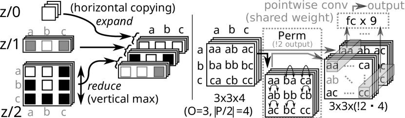
Figure 1: (Left) expand and reduce operations performed on a boolean MAPR containing nullary, unary, and binary predicates and three objects, a, b, and c. Each white / black square represents a boolean value (true / false). (Right) compose operation performed on 4 binary predicates. Each predicate is represented as a $3\times 3$ matrix, resulting in a $\mathbb{R}^{3\times 3\times 4}$ tensor. For a matrix, perm is equivalent to concatenating the matrix with its transposition, resulting in a $\mathbb{R}^{3\times 3\times(!2\cdot 4)}$ tensor. After perm, a shared fully-connected layer is applied to each combination of arguments (such an operation is sometimes called a pointwise convolution).

All three operations (expand, reduce, and compose) can be implemented as tensor operations over MAPRs (Figure 1). Given a binary tensor ${\bm{z}}/n$ of shape $O^{n}\times{\left|P/n\right|}$, expand copies the $n$-th axis to $n+1$-th axis resulting in a shape $O^{n+1}\times{\left|P/n\right|}$, and reduce takes the $\max$ of $n$-th axis resulting in a shape $O^{n-1}\times{\left|P/n\right|}$, representing $\exists$.

Finally, the compose operation combines the information between the neighboring tensors ${\bm{z}}/n,{\bm{z}}/_{n-1},{\bm{z}}/_{n+1}$. In order to use the information in the neighboring arities ($P$, $\underline{P}$ and $\overline{P}$), the input concatenates ${\bm{z}}/n$ with $\textsc{expand}({\bm{z}}/_{n-1})$ and $\textsc{reduce}({\bm{z}}/_{n+1})$, resulting in a shape $O^{n}\times C$ where $C={\left|P/n\right|}+{\left|P/_{n-1}\right|}+{\left|P/_{n+1}\right|}$. Next, a Perm function enumerates and concatenates the results of permuting the first $n$ axes in the tensor, resulting in a shape $O^{n}\times(!n\cdot C)$. It then applies a $n$-D pointwise convolutional filter $f_{n}$ with $Q$ output features, resulting in $O^{n}\times Q$, i.e., applying a fully connected layer to each vector of length $!n\cdot C$ while sharing the weights. It is activated by any nonlinearity $\sigma$ to obtain the final result, which is a sigmoid activation function in our implementation. We denote the result as $\textsc{compose}({\bm{z}},n,Q,\sigma)$. Formally, $\forall j\in 1..n,\forall o_{j}\in 1..O$,

$$({\bm{z}})=\textsc{perm}\Big{(}\textsc{expand}({\bm{z}}/_{n-1});\ {\bm{z}}/n;\ \textsc{reduce}({\bm{z}}/_{n+1})\Big{)},$$

$$\textsc{compose}({\bm{z}},n,Q,\sigma)_{o_{1}\cdots o_{n}}=\sigma(f_{n}(\Pi({\bm{z}})_{o_{1}\cdots o_{n}}))\in\mathbb{R}^{Q}.$$

An NLM contains $N$ (the maximum arity) compose operation for the neighboring arities, with appropriately omitting both ends ($0$ and $N+1$) from the concatenation. We denote the result as $\textsc{NLM}_{Q,\sigma}({\bm{z}})=(\textsc{compose}({\bm{z}},1,Q,\sigma),\cdots,\textsc{compose}({\bm{z}},N,Q,\sigma))$. These horizontal arity-wise compositions can be layered vertically, allowing the composition of predicates whose arities differ more than 1 (e.g., two layers of NLM can combine unary and quaternary predicates). Since $f_{n}$ is applied in a convolutional manner over $O^{n}$ object tuples, the number of weights in an NLM layer does not depend on the number of objects in the input. However, it is still affected by the number of predicates in the input, which alters $C$.

NLMs/GNNs/HGNs

We prefer NLMs over GNNs/HGNs for two reasons. First, unlike GNNs/HGNs, operations in NLMs have clear logical interpretations: $\forall/\exists$ (reduce / expand) and combining input formula with different arguments (compose). Next, the arity in NLMs’ hidden layers can be expand-ed arbitrarily large. GNNs are limited to binary/unary relations (edge/node-embeddings). The arity of a hidden HGN layer can be higher, but must match the input. FactorGNN (Zhang, Wu, and Lee 2020) is similar.

Value Function as NLMs

To represent a goal-generalized value function $V(s,G)$ with NLMs, we concatenate each element of two sets of binary arrays: One set representing the current state and another the goal conditions. The last dimension of each array in the resulting set is twice larger.

When the predicates in the input PDDL domain have a maximum arity $N$, we specify the maximum intermediate arity $M$ and the depth of NLM layers $L$ as a hyperparameter. The intermediate NLM layers expand the arity up to $M$ using expand operation, and shrink the arity near the output because a value function has a scalar (arity 0) output. For example, with $N=2$, $M=3$, $L=7$, the arity of each layer follows $(2,3,3,3,2,1,0)$. Higher arities are not necessary near the output because the information in each layer propagates only to the neighboring arities. Since each expand/reduce operation only increments/decrements the arity by one, $L,N,M$ must satisfy $N\leq M\leq L$. Intermediate conclusions in NLM is fixed to $Q=8$.

The output of this NLM is unactivated, similar to a regression task, because we use its raw value as the predicted correction to the heuristic function. In addition, we implement NLM with a skip connection that was popularized in ResNet image classification network (He et al. 2016): The input of $l$-th layer is a concatenation of the outputs of all previous layers. Due to the direct connections between the layers in various depths, the layers near the input receive more gradient information from the output, preventing the gradient vanishing problem in deep neural networks.

4 Experimental Evaluation

Our objective is to see whether our RL agent can improve the efficiency of a Greedy Best-First Search (GBFS), a standard algorithm for solving satisficing planning problems, over a domain-independent heuristic. The efficiency is measured by the number of node-evaluations performed during search. We also place an emphasis on generalization: We hope that NLMs are able to generalize from smaller training instances with fewer objects to instances with more objects.

We train our RL agent with rewards shaped by $h^{\text{FF}}$ and $h^{\text{add}}$ heuristics obtained from pyperplan library. We write blind heuristic $\forall s;h^{\text{blind}}(s)=1$ to denote a baseline without shaping. While our program is compatible with a wide range of unit-cost IPC domains (see the list of 25 domains in Appendix A.6), we focus on extensively testing its selected subset with a large enough number of independently trained models with different random seeds (20), to produce high-confidence results. This is because RL algorithms tend to have a large variance in their outcomes (Henderson et al. 2018), induced by sensitivity to initialization, randomization in exploration, and randomization in experience replay.

We trained our system on five domains in (Rivlin, Hazan, and Karpas 2019): 4-ops blocksworld, ferry, gripper, logistics, satellite, and three additional IPC domains: miconic, parking, and visitall. In all domains, we generated problem instances using existing parameterized generators (Fawcett et al. 2011). For each domain, we provided between 195 and 500 instances for training, and between 250 and 700 instances for testing. The generator parameters for test instances contain the ranges used for IPC instances (See Appendix Table 3). We remove trivial instances whose initial states satisfy the goals, which are produced by the generators occasionally, especially for small parameter values used for training instances. Each agent is trained for 50000 steps, which takes about 4 to 6 hours on Xeon E5-2600 v4 and Tesla K80. Hyperparameters can be found in Appendix A.5.

Baselines Ours (mean${{\pm}}$stderr (max) of 20 runs) GBFS GBFS GBFLS (incomparable) domain (total) $h^{\text{blind}}$ $h^{\text{add}}$ $h^{\text{FF}}$ $H^{\text{blind}}$ $H^{\text{add}}$ $H^{\text{FF}}$ -HGN -H -V (-H -V) blocks (250) 0 126 87 73.1${{\pm}}$2.8(94) 186.6${{\pm}}$7.5(229) 104${{\pm}}$1.5(114) 3 208 0 250 250 ferry (250) 0 138 250 40.4${{\pm}}$3.2(62) 233.9${{\pm}}$4(249) 0.4 250${{\pm}}$0(250) 27 240 0 250 250 gripper (250) 0 250 250 47.5${{\pm}}$5(85) 0.4 250${{\pm}}$0(250) 0.4 250${{\pm}}$0(250) 63 139 0 250 250 logistics (250) 0 106 243 0${{\pm}}$0(0) 54.1${{\pm}}$6.8(115) 79.8${{\pm}}$12.9(189) - 0 0 30 33 miconic (442) 171 442 442 143.3${{\pm}}$6.8(246) 0.4 442${{\pm}}$0(442) 0.4 440.8${{\pm}}$1.3(442) - 0 0 442 442 parking (700) 0 607 700 0.9${{\pm}}$0.2(3) 619${{\pm}}$32.4(689) 0.4 696.9${{\pm}}$0.5(700) - 333 0 403 357 satellite (250) 0 249 222 26.5${{\pm}}$5(99) 0.4 233.3${{\pm}}$5.2(250) 163.2${{\pm}}$11(205) - 9 0 137 135 visitall (252) 252 252 252 207.6${{\pm}}$5.3(238) 0.4 251.9${{\pm}}$0.1(252) 0.4 252${{\pm}}$0(252) - 101 0 249 249

Table 1: Coverage of GBFS with 100,000 node evaluations limit. Our scores are highlighted in bold and underline when our average score is significantly better/worse than the baseline ($|\text{ours}-\text{baseline}|>\text{stderr}$, where $\text{stderr}=\frac{\text{stdev}}{\sqrt{20}}$). Some scores are 0.4 marked for caution when both ours and baselines solved nearly all instances. They were too easy to measure coverage differences, and thus the lack thereof does not imply the lack of improvement in the heuristics. Instead, node evaluation plots (Figure 2) show reduction in the search effort. In conclusion, our approach generally improves the performance in many domains except logistics, where only the best seed of $h^{\text{add}}$ managed to improve upon the baseline (106 $\rightarrow$ 115).

$H^{\text{blind}}$ $h^{\text{blind}}$ $H^{\text{add}}$ $h^{\text{add}}$ $H^{\text{FF}}$ $h^{\text{FF}}$ blocks 94 0 224 5 109 9 ferry 62 0 249 0 250 0 gripper 85 0 250 0 200 50 logistics 0 0 108 14 167 77 miconic 234 17 381 61 442 0 parking 2 0 508 105 484 173 satellite 93 0 115 110 155 63 visitall 192 60 216 36 192 59

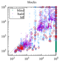
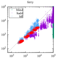
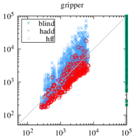
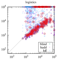
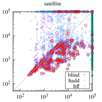
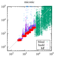
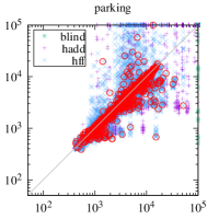
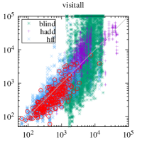
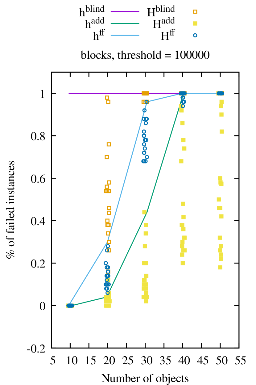
Figure 2: Best viewed on computer screens. (Left) Number of instances where $\textsc{GBFS}(H)$ had less evaluations than $\textsc{GBFS}(h)$ did (and vice versa), excluding ties and instances failed by both. $\textsc{GBFS}(H)$ is a result of the best training seed with the least sum of evaluations across the instances in a domain. They show that RL improves the performance both with ($H^{\text{FF}},H^{\text{add}}$) and without ($H^{\text{blind}}$) reward shaping in the best case. (Middle) Scatter plot showing the number of node evaluations on 8 domains, where $x$-axis is for GBFS with $h^{\text{blind}},h^{\text{FF}},h^{\text{add}}$ and $y$-axis is for $H^{\text{blind}},H^{\text{FF}},H^{\text{add}}$. Each point corresponds to a single test problem instance. Results of 20 random seeds are plotted against a single deterministic baseline. Failed instances are plotted on the border. Red points highlight the best seed from $H^{\text{FF}}$. (Right) The rate of finding a solution ($y$-axis) for blocks instances and the number of objects ($x$-axis), demonstrating that the improvements generalize to larger instances. The agents are trained on 2-6 objects while the test instances contain 10-50 objects (Table 3). Results on other domains are in the appendix (Figure 3).

We ran GBFS on the test instances using $-V(s,G)=-\hat{V}(s,G)+h_{\gamma}(s)$ as a heuristics. (Discounting does not affect the expansion order in GBFS and unit cost domains.) Instead of setting time or memory limits, we limited the maximum node evaluations in GBFS to 100,000. If a problem was solved within the limit, the configuration gets the score 1 for that instance, otherwise it gets 0. The sum of the scores for each domain is called the coverage in that domain. Table 1 shows the coverage in each of the tested domains, comparing our configurations to the baselines, as well as to the prior work (Section 4). The baselines are denoted by their heuristic (e.g., $h^{\text{FF}}$ is the GBFS with $h^{\text{FF}}$), while our heuristics, obtained by a training with reward shaping $\phi=-h_{\gamma}$, are denoted with a capital $H$ (e.g., $H^{\text{FF}}$). Additionally, Figure 2 goes beyond the pure coverage and compares the node evaluations. These results answer the following questions:

(Q1) Do our agents learn heuristic functions at all, i.e., is $\textsc{gbfs}(h^{\text{blind}})<\textsc{gbfs}(H^{\text{blind}})$ (green dots in Figure 2), where $\textsc{gbfs}(h^{\text{blind}})$ is similar to breadth-first search with duplicate detection, and $\textsc{gbfs}(H^{\text{blind}})$ is baseline RL without reward shaping? With the exception of visitall and miconic, $\textsc{gbfs}(h^{\text{blind}})$ could not solve any instances in the test set, while using the heuristics learned without shaping ($\textsc{gbfs}(H^{\text{blind}})$) significantly improved coverage in 5 of the 6 domains.

(Q2) Do they improve over the baselines they were initialized with, i.e., is $\textsc{gbfs}(h)<\textsc{gbfs}(H)$? In domains where they did not solve every instances (blocks, ferry, logistics, parking, satellite), Table 1 suggests that the reward-shaping-based training has successfully improved the coverage in blocks, ferry, parking. Since the number of solved instances is not a useful metric in domains where both configurations solved nearly all instances (lack of coverage improvement does not imply lack of improvement in efficiency), we next compare the number of node evaluations, which directly evaluates the search efficiency. Figure 2 shows that the search effort tends to be reduced, especially on the best seed. However, this is sensitive to the random seed, and the improvement is weak on logistics. These results suggest that while RL can improve the planning efficiency, we need several iterations of random experiments to achieve improvements due to the high randomness of RL.

(Q3) Do our agents with reward shaping outperform our agents without shaping? According to Table 1, $H^{\text{FF}}$ and $H^{\text{add}}$ outperforms $H^{\text{blind}}$. Notice that $h^{\text{FF}}$ and $h^{\text{add}}$ also outperform $h^{\text{blind}}$. This suggest that the informativeness of the base heuristic used for reward shaping affects the quality of the learned heuristic. This matches the theoretical expectation: The potential function plays the role of domain knowledge that initializes the policy.

(Q4) Did heuristics accelerate exploration during training and contribute to the improvement? Table 2 shows the number of goals reached during training, indicating that reward shaping helps the agent receive real rewards at goals more often. See Appendix Figure 4-5 for cumulative plots.

(Q5) Do the learned heuristics maintain their improvement in larger problem instances, i.e., do they generalize to more objects? Figure 2 (Right) plots the number of objects ($x$-axis) and the ratio of success ($y$-axis) over blocks instances. The agents are trained on 2-6 objects while evaluated on 10-50 objects. It shows that the heuristic accuracy is improved in instances whose size far exceeds the training instances for $h^{\text{blind}},h^{\text{FF}},h^{\text{add}}$. Due to space limitations, plots for the remaining domains are in Appendix, Figure 3.

domain	$h^{\text{blind}}$	$h^{\text{add}}$	$h^{\text{FF}}$
blocks	362$\pm$42	527$\pm$58	621$\pm$31
ferry	516$\pm$52	976$\pm$19	949$\pm$21
gripper	275$\pm$33	673$\pm$18	600$\pm$20
logistics	93$\pm$21	502$\pm$33	488$\pm$32
miconic	542$\pm$18	708$\pm$9	722$\pm$9
parking	400$\pm$51	809$\pm$24	814$\pm$27
satellite	212$\pm$37	658$\pm$34	654$\pm$26
visitall	211$\pm$22	198$\pm$20	350$\pm$17

Table 2: The cumulative number of goal states the agent has reached during training. The numbers are average and standard deviation over 20 seeds. Best numbers among heuristics are highlighted in bold, with ties equally highlighted when there are no statistically significant differences between them under Wilcoxon’s rank-sum test ($p\geq 0.05$). The results indicate that reward shaping significantly accelerates the exploration compared to no shaping ($h^{\text{blind}}$).

Comparison with Previous Work

Next, we compared our learned heuristics with two recent state-of-the-art learned heuristics. The first approach, STRIPS-HGN (Shen, Trevizan, and Thiébaux 2020), is a supervised learning method that can learn domain-dependent or domain-independent heuristics depending on the dataset. It uses hypergraph networks (HGN), a generalization of Graph Neural Networks (GNNs) (Scarselli et al. 2009). The authors have provided us with pre-trained weights for three domains: gripper, ferry, and blocksworld for the domain-dependent setting. STRIPS-HGN was originally developed and evaluated for use with $A^{*}$, for obtaining near-optimal plans. Since we do not optimize plan quality in this work, we instead use it with GBFS, which helps finding the goal more quickly possibly at the expense of plan quality and is the same algorithm we use for our heuristics. We recognize it may not have been designed for this scenario and that therefore may not best demonstrate its strengths. It remains useful as a baseline point of comparison for our work. We denote this variant GBFS-HGN.

The second approach we compare to is GBFS-GNN (Rivlin, Hazan, and Karpas 2019), an RL-based heuristic learning method that trains a GNN-based value function. The authors use Proximal Policy Optimization (Schulman et al. 2017), a state of the art RL method that stabilizes the training by limiting the amount of policy change in each step (the updated policy stays in the proximity of the previous policy). The value function $V(s)$ is a GNN optionally equipped with attentions (Veličković et al. 2018; Vaswani et al. 2017). In addition, the authors proposed to adjust $V(s)$ by the policy $\pi(a|s)$ and its entropy $H_{\pi}=\sum_{a}\pi(a|s)\log\pi(a|s)$. The heuristic value of the successor state $s^{\prime}=a(s)$ is given by $h(s^{\prime})=\frac{\pi(a|s)V(s)}{1+H_{\pi}}$. We call it an $H$-adjusted value function.

The authors also proposed a variant of GBFS which launches a greedy informed local search after each expansion. We distinguish their algorithmic improvement and the heuristics improvement by naming their search algorithm as Greedy Best First Lookahead Search (GBFLS). Our formal rendition of GBFLS can be found in Appendix A.2.

We counted the number of test instances that are solved by these approaches within 100,000 node evaluations. In the case of GBFLS, the evaluations also include the nodes that appear during the lookahead. We evaluated GBFS-HGN on the domains where pretrained weights are available. For GBFS-GNN, we obtained the source code from the authors (private communication) and minimally modified it to train on the same training instances that we used for our approach. We evaluated 4 variants of GBFS-GNN: GBFS-H, GBFS-V, GBFLS-H, and GBFLS-V, where “H” denotes $H$-adjusted value function, and “V” denotes the original value function. Note that fair evaluation should compare our method with GBFS-H/V, not GBFLS-H/V.

Table 1 shows the results. We first observe that large part of the success of GBFS-GNN should be attributed to the lookahead extension of GBFS. This is because the score is GBFLS-V $\gg$ GBFS-H $\gg$ GBFS-V, i.e., GBFLS-V performs very well even with a bad heuristics ($V(s)$). While we report the coverage for both GBFLS-H/V and GBFS-H/V, the configurations that are comparable to our setting are GBFS-H/V. First, note that GBFS-HGN is significantly outperformed by all other methods. Comparing to the other two, both $H^{\text{add}}$ and $H^{\text{FF}}$ outperform GBFS-H in 7 out of the 8 domains, losing only on blocks. It is worth noting that $H^{\text{blind}}$ outperforms GBFS-H in miconic, satellite, and visitall. Since both $H^{\text{blind}}$ and GBFS-H are trained without reward shaping, the difference is due to the network shape (NLM vs GNN) and the training (Modified RTDP vs PPO).

5 Related Work

Early attempts to learn heuristics include shallow, fully connected neural networks (Arfaee, Zilles, and Holte 2011), its online version (Thayer, Dionne, and Ruml 2011), combining SVMs (Cortes and Vapnik 1995) and NNs (Satzger and Kramer 2013), learning a residual from heuristics (Yoon, Fern, and Givan 2008), or learning a relative ranking between states (Garrett, Kaelbling, and Lozano-Pérez 2016). More recently, Ferber, Helmert, and Hoffmann (2020) tested fully-connected layers in modern frameworks. ASNet (Toyer et al. 2018) learns domain-dependent heuristics using a GNN-like network. They are based on supervised learning methods that require the high-quality training dataset (accurate goal distance estimates of states) that are prepared separately. Our RL-based approaches explore the environment by itself to collect data, which is automated (pros) but could be sample-inefficient (cons).

A large body of work utilize ILP techniques to learn a value function (Gretton and Thiébaux 2004) features (Wu and Givan 2010), pruning rules (Krajnanský et al. 2014), or a policy function by classifying the best action (Fern, Yoon, and Givan 2006). NLM is a differentiable ILP system that subsumes first-order decision lists / trees used in ILP.

Other RL-based approaches include Policy Gradient with FF to accelerate exploration for probabilistic PDDL (Buffet, Aberdeen et al. 2007), and PPO-based Meta-RL (Duan et al. 2016) for PDDL3.1 discrete-continuous hybrid domains (Gutierrez and Leonetti 2021). They do not use reward shaping, thus our contributions are orthogonal.

Grounds and Kudenko (2005) combined RL and STRIPS planning with reward shaping, but in a significantly different setting: They treat a 2D navigation as a two-tier hierarchical problem where unmodified FF (Hoffmann and Nebel 2001) or Fast Downward (Helmert 2006) are used as high-level planner, then their plans are used to shape the rewards for the low-level RL agent. They do not train the high-level planner.

6 Conclusion

In this paper, we proposed a domain-independent reinforcement learning framework for learning domain-specific heuristic functions. Unlike existing work on applying policy gradient to planning (Rivlin, Hazan, and Karpas 2019), we based our algorithm on value iteration. We addressed the difficulty of training an RL agent with sparse rewards using a novel reward-shaping technique which leverages existing heuristics developed in the literature. We showed that our framework not only learns a heuristic function from scratch ($H^{\text{blind}}$), but also learns better if aided by heuristic functions (reward shaping). Furthermore, the learned heuristics keeps outperforming the baseline over a wide range of problem sizes, demonstrating its generalization over the number of objects in the environment.

Appendix A Appendix

A.1 Domain-Independent Heuristics for Classical Planning

In this section, we discuss various approximations of delete-relaxed optimal cost $h^{+}(s)$. Given a classical planning problem ${\left<P,O,A,I,G\right>}$, and a state $s$, each heuristics is typically implicitly conditioned by the goal condition. $h^{\text{add}}$ heuristics is recursively defined as follows:

$$h^{\text{add}}(s,G)=\sum_{p\in G}\left\{\begin{array}[]{l}0\ \text{if}\ p\in s.\ \text{Otherwise,}\\ \min_{{\left\{a\in A\mid p\in\textsc{add}(a)\right\}}}\\ \qquad\left[\textsc{cost}(a)+h^{\text{add}}(s,\textsc{pre}(a))\right].\\ \end{array}\right.$$ (9)

$h^{\text{FF}}$ heuristics can be defined based on $h^{\text{add}}$ as a subprocedure. The action $a$ which minimizes the second case ($p\not\in S$) of each of the definition above is conceptually a “cheapest action that achieves a subgoal $p$ for the first time”, which is called a cheapest achiever / best supporter $\text{bs}(p,s)$ of $p$. Using $h$ and its best supporter function, $h^{\text{FF}}$ is defined as follows:

$$h^{\text{FF}}(s,G) =\sum_{a\in\text{RelaxedPlan}(s,G)}\textsc{cost}(a)$$ (10)

$$\text{RelaxedPlan}(s,G) =\bigcup_{p\in G}\left\{\begin{array}[]{l}\emptyset\ \text{if}\ p\in s.\ \text{Otherwise,}\\ {\left\{a\right\}}\cup\text{RelaxedPlan}(s,\textsc{pre}(a))\\ \qquad\text{where}\ a=\text{bs}(p,s).\end{array}\right.$$ (14)

$$\text{bs}(p,s) =\operatorname*{arg\,min}_{{\left\{a\in A\mid p\in\textsc{add}(a)\right\}}}\left[\textsc{cost}(a)+h^{\text{add}}(s,\textsc{pre}(a))\right].$$ (15)

A.2 Greedy Best First Search and Greedy Best First Lookahead Search (Rivlin, Hazan, and Karpas 2019)

Given a classical planning problem ${\left<P,O,A,I,G\right>}$, we define its state space as a directed graph $(V,E)$ where $V=2^{P(O)}$, i.e., a power set of subsets of propositions $P(O)$. Greedy Best First Search is a greedy version of $A^{*}$ algorithm (Hart, Nilsson, and Raphael 1968), therefore we define $A^{*}$ first.

We follow the optimized version of the algorithm discussed in Burns et al. (2012) which does not use CLOSE list and avoids moving elements between CLOSE list and OPEN list by instead managing a flag for each search state. Let $f(s)=g(s)+h(s)$ be a function that computes the sum of $h(s)$ and $g(s)$, where $g(s)$ is a value stored for each state which represents the currently known upper bound of the shortest path cost from the initial state $I$. For every state $s$, $g(s)$ is initialized to infinity except $g(I)=0$. Whenever a state $s$ is expended, $f(s)$ is a lower bound of the path cost that goes through $s$. $A^{*}$ algorithm is defined as in Algorithm 2. We simplified some aspects such as updating the parent node pointer, the rules for tiebreaking, or extraction of the plan by backtracking the parent pointers. Notice that the update rule for $g$-values in $A^{*}$ is a Bellman update specialized for a positive cost function.

1:  Priority queue $\text{OPEN}\leftarrow\emptyset$.

2:  $g(s)\leftarrow\infty$ for all $s\in V$ except $g(I)\leftarrow 0$.

3:  $s$.closed $\leftarrow\bot$ for all $s\in V$.

4:  $\text{OPEN}.\textsc{push}(I,f(I))$

5:  while $\text{OPEN}\not=\emptyset$ do

6:     State $s\leftarrow\text{OPEN}.\textsc{popmin}()$ Expansion

7:     if $s\supseteq G$ then

8:        return  $s$

9:     if $s$.closed $=\top$ then

10:        continue

11:     else

12:        $s$.closed $\leftarrow\top$

13:     for $a\in{\left\{a\in A\mid\textsc{pre}(a)\subseteq s\right\}}$  do

14:        successor $t=a(s)$ Note: Appropriate caching of $t$ is necessary.

15:        if $g(t)>\textsc{cost}(a)+g(s)$ then

16:           $g(t)\leftarrow\textsc{cost}(a)+g(s)$ Bellman update

17:           $t$.closed $\leftarrow\bot$ Reopening

18:           $\text{OPEN}.\textsc{push}(t,f(t))$

Algorithm 2 $A^{*}$ algorithm for a planning problem ${\left<P,O,A,I,G\right>}$ with state space $(V,E)$.

Three algorithms can be derived from $A^{*}$ by redefining the sorting key $f(s)$ for the priority queue OPEN. First, ignoring the heuristic function by redefining $f(s)=g(s)$ yields Dijkstra’s search algorithm. Another is weighted $A^{*}$ (Pohl 1970), where we redefine $f(s)=g(s)+w\cdot h(s)$ for some value $w\geq 1$, which results in trusting the heuristic guidance relatively more greedily.

As the extreme version of WA*, conceptually $w\rightarrow\infty$ yields the Greedy Best First Search algorithm (Russell et al. 1995) which completely greedily trusts the heuristic guidance. In practice, we implement it by ignoring the $g(s)$ value, i.e., $f(s)=h(s)$. This also simplifies some of the conditionals in Algorithm 2: There is no need for updating the $g$ value, or reopening the node. In addition, purely satisficing algorithm like GBFS can enjoy an additional enhancement called early goal detection. In $A^{*}$, the goal condition is checked when the node is popped from the OPEN list (line 7) – if we detect the goal early, it leaves the possibility that it returns a suboptimal goal node. In contrast, since we do not have this optimality requirement in GBFS, the goal condition can be checked in line 12 where the successor state is generated. GBFS is thus defined as in Algorithm 3.

1:  Priority queue $\text{OPEN}\leftarrow\emptyset$.

2:  $s$.closed $\leftarrow\bot$ for all $s\in V$.

3:  $\text{OPEN}.\textsc{push}(I,h(I))$

4:  while $\text{OPEN}\not=\emptyset$ do

5:     State $s\leftarrow\text{OPEN}.\textsc{popmin}()$ Expansion

6:     if $s$.closed $=\top$ then

7:        continue

8:     else

9:        $s$.closed $\leftarrow\top$

10:     for $a\in{\left\{a\in A\mid\textsc{pre}(a)\subseteq s\right\}}$  do

11:        successor $t=a(s)$ Note: Appropriate caching of $t$ is necessary.

12:        if $t\supseteq G$ then

13:           return  $t$ Early goal detection.

14:        $\text{OPEN}.\textsc{push}(t,h(t))$

Algorithm 3 GBFS algorithm for a planning problem ${\left<P,O,A,I,G\right>}$ with state space $(V,E)$.

Finally, Rivlin, Hazan, and Karpas (2019) proposed an unnamed extension of GBFS which performs a depth-first lookahead after a node is expanded. We call the search algorithm Greedy Best First Lookahead Search (GBFLS), defined in Algorithm 4. We perform the same early goal checking during the lookahead steps. Note that the nodes are added only when the current node is expanded; Nodes that appear during the lookahead are not added to the OPEN list. However, these nodes must be counted as evaluated node because it is subject to goal checking and because we evaluate their heuristic values. The lookahead has an artificial depth limit $D$ which is defined as $D=5\cdot h^{\text{FF}}(I)$, i.e., 5 times the value of the FF heuristics at the initial state. When $h^{\text{FF}}(I)=\infty$, the limit is set to 50, according to their code base.

1:  Priority queue $\text{OPEN}\leftarrow\emptyset$.

2:  $s$.closed $\leftarrow\bot$ for all $s\in V$.

3:  $\text{OPEN}.\textsc{push}(I,h(I))$

4:  while $\text{OPEN}\not=\emptyset$ do

5:     State $s\leftarrow\text{OPEN}.\textsc{popmin}()$ Expansion

6:     if $s$.closed $=\top$ then

7:        continue

8:     else

9:        $s$.closed $\leftarrow\top$

10:     for depth $d<D$ do

11:        for $a\in{\left\{a\in A\mid\textsc{pre}(a)\subseteq s\right\}}$  do

12:           successor $t=a(s)$ Note: Appropriate caching of $t$ is necessary.

13:           if $t\supseteq G$ then

14:              return  $t$ Early goal detection.

15:           $\text{OPEN}.\textsc{push}(t,h(t))$ if $d=0$

16:        $a\leftarrow\operatorname*{arg\,min}_{a}h(a(s))$

17:        $s\leftarrow a(s)$

Algorithm 4 GBFLS algorithm for a planning problem ${\left<P,O,A,I,G\right>}$ with state space $(V,E)$.

A.3 Implementation

Our implementation combines the jax auto-differentiation framework for neural networks, and pyperplan for parsing and to obtain the heuristic value of $h^{\text{FF}}$ and $h^{\text{add}}$.

A.4 Generator Parameters

Table 3 contains a list of parameters used to generate the training and testing instances. Since generators have a tendency to create an identical instance especially in smaller parameters, we removed the duplicates by checking the md5 hash value of each file.

Domain	Parameters	$|O|$
blocks/train/	2-6 blocks x 50 seeds	2-6
blocks/test/	10,20,..,50 blocks x 50 seeds	10-50
ferry/train/	2-6 locations x 2-6 cars x 50 seeds	4-7
ferry/test/	10,15,…30 locations and cars x 50 seeds	20-60
gripper/train/	2,4…,10 balls x 50 seeds (initial/goal locations are randomized)	6-14
gripper/test/	20,40,…,60 balls x 50 seeds (initial/goal locations are randomized)	24-64
logistics/train/	1-3 airplanes x 1-3 cities x 1-3 city size x 1-3 packages x 10 seeds	5-13
logistics/test/	4-8 airplanes/cities/city size/packages x 50 seeds	32-96
satellite/train/	1-3 satellites x 1-3 instruments x 1-3 modes x 1-3 targets x 1-3 observations	15-39
satellite/test/	4-8 satellites/instruments/modes/targets/observations x 50 seeds	69-246
miconic/train/	2-4 floors x 2-4 passengers x 50 seeds	8-12
miconic/test/	10,20,30 floors x 10,20,30 passengers x 50 seeds	24-64
parking/train/	2-6 curbs x 2-6 cars x 50 seeds	8-16
parking/test/	10,15,..,25 curbs x 10,15,..25 cars x 50 seeds	24-54
visitall/train/	For $n\in 3..5$, $n$x$n$ grids, 0.5 or 1.0 goal ratio, $n$ blocked locations, 50 seeds	8-22
visitall/test/	For $n\in 6..8$, $n$x$n$ grids, 0.5 or 1.0 goal ratio, $n$ blocked locations, 50 seeds	32-58

Table 3: List of parameters used for generating the training and testing instances.

A.5 Hyperparameters

We trained our network with a following set of hyperparameters: Maximum episode length $D=40$, Learning rate 0.001, discount rate $\gamma=0.999999$, maximum intermediate arity $M=3$, number of layers $L=4$ in satellite and logistics, while $L=6$ in all other domains, the number of features in each NLM layer $Q=8$, batch size 25, temperature $\tau=1.0$ for a policy function (Section 2.2), replay buffer size $|B|=6000$, and the total number of SGD steps to 50000, which determines the length of the training. We used $L=4$ for those two domains to address GPU memory usage: Due to the size of the intermediate layer $O^{n}\times(n!\cdot C)$, NLM sometimes requires a large amount of GPU memory. Each training takes about 4 to 6 hours, depending on the domain.

A.6 Preliminary Results on Compatible Domains

We performed a preliminary test on a variety of IPC classical domains that are supported by our implementation. The following domains worked without errors: barman-opt11-strips, blocks, depot, driverlog, elevators-opt11+sat11-strips, ferry, floortile-opt11-strips, freecell, gripper, hanoi, logistics00, miconic, mystery, nomystery-opt11-strips, parking-opt11+sat11-strips, pegsol-opt11-strips, pipesworld-notankage, pipesworld-tankage, rovers, satellite, scanalyzer-08-strips, sokoban-opt11-strips, tpp, transport-opt11+sat08-strips, visitall-opt11-strips, zenotravel.

A.7 Full Results

Figure 3 contains the full results of Figure 2 (Right).

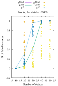
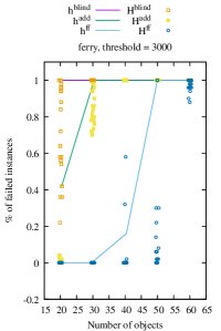
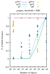
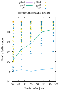
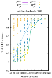
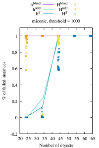
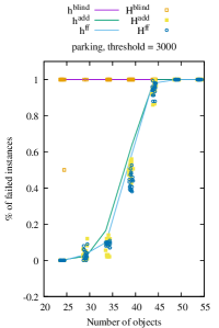
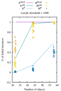
Figure 3: The rate of successfully finding a solution ($y$-axis) for instances with a certain number of objects ($x$-axis). Learned heuristic functions outperform their original baselines used for reward shaping in most domains. Since the initial maximum node evaluation is too permissive, we manually set a threshold for the number of node evaluations for each domain and filtered the instances when the node evaluation exceeded this threshold. This filtering emphasizes the difference because both the learned and the baseline variants may have solved all instances.

Figure 4: Cumulative number of instances that are solved during the training, where $x$-axis is the training step (part 1). Note that this may include solving the same instance multiple times.

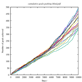
Figure 5: Cumulative number of instances that are solved during the training, where $x$-axis is the training step (part 2). Note that this may include solving the same instance multiple times.

References

- Arfaee, Zilles, and Holte (2011) Arfaee, S. J.; Zilles, S.; and Holte, R. C. 2011. Learning Heuristic Functions for Large State Spaces. Artif. Intel., 175(16-17).
- Asai and Fukunaga (2015) Asai, M.; and Fukunaga, A. 2015. Solving Large-Scale Planning Problems by Decomposition and Macro Generation. In ICAPS.
- Badia et al. (2020) Badia, A. P.; Piot, B.; Kapturowski, S.; Sprechmann, P.; Vitvitskyi, A.; Guo, Z. D.; and Blundell, C. 2020. Agent57: Outperforming the Atari Human Benchmark. In ICML. PMLR.
- Buffet, Aberdeen et al. (2007) Buffet, O.; Aberdeen, D.; et al. 2007. FF+FPG: Guiding a Policy-Gradient Planner. In ICAPS.
- Burns et al. (2012) Burns, E. A.; Hatem, M.; Leighton, M. J.; and Ruml, W. 2012. Implementing Fast Heuristic Search Code. In SOCS.
- Bylander (1994) Bylander, T. 1994. The Computational Complexity of Propositional STRIPS Planning. Artif. Intel., 69(1).
- Cortes and Vapnik (1995) Cortes, C.; and Vapnik, V. 1995. Support-Vector Networks. Mach. Learn., 20(3).
- Dong et al. (2019) Dong, H.; Mao, J.; Lin, T.; Wang, C.; Li, L.; and Zhou, D. 2019. Neural Logic Machines. In ICLR.
- Duan et al. (2016) Duan, Y.; Schulman, J.; Chen, X.; Bartlett, P. L.; Sutskever, I.; and Abbeel, P. 2016. RL2: Fast Reinforcement Learning via Slow Reinforcement Learning. CoRR, abs/1611.02779.
- Fawcett et al. (2011) Fawcett, C.; Helmert, M.; Hoos, H.; Karpas, E.; Röger, G.; and Seipp, J. 2011. FD-Autotune: Domain-Specific Configuration using Fast Downward. In PAL.
- Ferber, Helmert, and Hoffmann (2020) Ferber, P.; Helmert, M.; and Hoffmann, J. 2020. Neural Network Heuristics for Classical Planning: A Study of Hyperparameter Space. In ECAI.
- Fern, Khardon, and Tadepalli (2011) Fern, A.; Khardon, R.; and Tadepalli, P. 2011. The First Learning Track of the International Planning Competition. Mach. Learn., 84(1-2).
- Fern, Yoon, and Givan (2006) Fern, A.; Yoon, S.; and Givan, R. 2006. Approximate Policy Iteration with a Policy Language Bias: Solving Relational Markov Decision Processes. J. Artif. Intell. Res., 25.
- Fikes and Nilsson (1972) Fikes, R. E.; and Nilsson, N. J. 1972. STRIPS: A New Approach to the Application of Theorem Proving to Problem Solving. Artif. Intel., 2(3).
- Garrett, Kaelbling, and Lozano-Pérez (2016) Garrett, C. R.; Kaelbling, L. P.; and Lozano-Pérez, T. 2016. Learning to Rank for Synthesizing Planning Heuristics. In IJCAI.
- Gretton and Thiébaux (2004) Gretton, C.; and Thiébaux, S. 2004. Exploiting First-Order Regression in Inductive Policy Selection. In UAI.