The Scott-Vogelius method for the Stokes problem on anisotropic meshes

Abstract

This paper analyzes the Scott-Vogelius divergence-free element pair on anisotropic meshes. We explore the behavior of the inf-sup stability constant with respect to the aspect ratio on meshes generated with a standard barycenter mesh refinement strategy, as well as a newly introduced incenter refinement strategy. Numerical experiments are presented which support the theoretical results.

1 Introduction

Let $\Omega\subset\mathbb{R}^{2}$ be a regular open polygon with boundary $\Gamma$. We consider the Stokes equation with the no-slip boundary condition:

$$-\nu\Delta\bm{u}+\nabla p ={\bm{f}}\text{ in }\Omega,$$

$$\nabla\cdot\bm{u} =0\text{ in }\Omega,$$

$$\bm{u} =0\text{ on }\Gamma,$$

where $\bm{u}$ is the velocity, $p$ is the pressure, ${\bm{f}}$ is a given body force, and $\nu$ is the viscosity.

In this manuscript we study the stability of the divergence-free Scott-Vogelius (SV) finite element pair on anisotropic meshes for the Stokes problem; the results trivially extend to other divergence free equations, e.g., the incompressible Navier-Stokes equations. Divergence-free methods and other pressure-robust schemes are an extremely active field of research (cf. [24, 31]) ranging from a variety of finite element pairs (e.g., [34, 9, 36, 16, 1, 15, 21, 18, 20]) to modifying the formulation of the equations (e.g., [27, 14, 28, 29, 26, 35, 25]). Advantages of divergence-free methods include exact enforcement of conservation laws, pressure robustness with the velocity error being independent of the pressure error and viscosity term [24, 3], and improved stability and accuracy of timestepping schemes [11, 17].

The Stokes equation has been studied on anisotropic meshes for a number of different element pairs. In [8] it was shown that for the Crouzeix-Raviart element, the inf-sup constant is independent of the aspect ratio on triangular and tetrahedral meshes. A similar result was shown for the Bernardi-Raugel finite element pair in two dimensions for classes of triangular and quadrilateral meshes in [7]. Recently, in [10] it was shown for a specific class of anisotropic triangulation that the lowest order Taylor-Hood element was uniformly inf-sup stable. A nonconforming pressure robust method was studied in [6]. Stability and convergence on anisotropic meshes for the Stokes equation has also been studied extensively for the hp-finite element method [4, 32, 33].

Up to this point there have been no theoretical results for $H^{1}$ conforming divergence free finite elements on anisotropic meshes. The low-order SV element pair is somewhat unique in that it is not inf-sup stable on general meshes, but requires special meshes e.g., the barycenter refinement (or Clough-Tocher refinement) which is obtained by connecting the vertices of each triangle on a given mesh to its barycenter. As pointed out in [23, p.12] this gives rise to meshes with possibly very small and large angles. The impact of these angles on the inf-sup constant was stated as an open problem in [23].

In this work we show barycenter refinement on anisotropic meshes will necessarily lead to large angles and propose an alternative mesh refinement strategy based on the incenter of each triangle. This incenter refinement strategy produces a mesh that avoids large angles and allows a smaller increase in aspect ratio on refinement. We prove there is a linear relationship between the inf-sup constant and the inverse of the aspect ratio for both the barycenter and incenter refined mesh; numerical experiments show that these results are sharp. Surprisingly, numerical tests indicate that there is not a significant difference, in terms of accuracy, between the incenter and barycenter refinement.

The rest of this manuscript is organized as follows: In Section 2 we introduce notation and give some preliminary results that will be used for the inf-sup stability estimates. We also prove that the incenter refined mesh has superior aspect ratios and angles compared to the barycenter refined mesh. In Section 3 we prove that the inf-sup constant scales linearly with the inverse of the aspect ratio for both barycenter and incenter refinement. In Section 4, we verify numerically the geometric results proven in Section 2 and stability results proven in Section 3. We also demonstrate that there does not appear to be an appreciable difference in terms of accuracy for the incenter versus barycenter refinement. Finally, the appendix contains proofs of some technical lemmas.

2 Preliminaries

Let $\mathcal{T}_{h}$ denote a conforming simplicial triangulation of $\Omega\subset\mathbb{R}^{2}$. We denote the vertices and edges of $T$ as $\{z_{i}\}_{i=1}^{3}$ and $\{e_{i}\}_{i=1}^{3}$ respectively, labeled such that $z_{i}$ is opposite of $e_{i}$. Set $h_{i}=|e_{i}|$ and without loss of generality, we assume $h_{1}\leq h_{2}\leq h_{3}$. We denote by $\rho_{T}$ the diameter of the incircle of $T$ and set $h_{T}=h_{3}$. Let $\alpha_{i}$ be the angle of $T$ at vertex $z_{i}$, note that $\alpha_{1}\leq\alpha_{2}\leq\alpha_{3}$.

Let $z_{0}\in T$ be an interior point of $T$, and set $T^{ct}=\{K_{1},K_{2},K_{3}\}$ to be the local (Clough-Tocher) triangulation of $T$, obtained by connecting the vertices of $T$ to $z_{0}$. The three triangles $\{K_{i}\}_{i=1}^{3}$ are labeled such that ${\partial}K_{i}\cap{\partial}T=e_{i}$. Let $a_{T}$ be the altitude of $T$ with respect to edge $e_{3}$, and let $k_{i}$ be the altitude of $K_{i}$ with respect to $e_{i}$ (cf. Figure 1).

2.1 Geometric results and dependence of split point

We examine the dependencies and properties of the local triangulation of $T$ on the choice of split point $z_{0}$. In particular, we consider geometric properties of the triangulations obtained by connecting vertices of $T$ to the barycenter and the incenter of $T$. First, we require a few definitions.

Definition 1.

The barycenter of $T$ is given by

$$z_{{\rm bary}}=\frac{1}{3}(z_{1}+z_{2}+z_{3}).$$

The incenter of $T$ is given by

$$z_{{\rm inc}}=\frac{1}{|{\partial}T|}(h_{1}z_{1}+h_{2}z_{2}+h_{3}z_{3}).$$

Definition 2.

1. The aspect ratio of $T$ is given by

   $${\varrho}_{T}:=\frac{h_{T}}{\rho_{T}}=\frac{|{\partial}T|h_{T}}{4|T|}.$$

2. The aspect ratio of $T^{ct}$, denoted by ${\varrho}_{T^{ct}}$, is defined as the maximum of the aspect ratio of the three triangles in the refinement, i.e.,

   $${\varrho}_{T^{ct}}:=\max_{K_{i}\in T^{ct}}{\varrho}_{K_{i}}.$$

Definition 3 ([2]).

A triangle $T$ is said to satisfy a large angle condition, written as $LAC(\delta)$, if there exists $\delta>0$ such that $\alpha_{i}<\pi-\delta$ for $i=1,2,3$.

Fig. 1: The Clough–Tocher split of a single triangle taking the split point $z_{0}$ to be the incenter (left) and barycenter (right).

Lemma 4.

Let the split point be taken to be the barycenter, i.e., $z_{0}=z_{{\rm bary}}$. Then as the aspect ratio of $T$ goes to infinity, the largest angle in $K_{3}$ goes to $\pi$, i.e., the large angle condition will be violated in $T^{ct}$ regardless of the angles of $T$.

Proof.

Recall the labeling assumption $h_{1}\leq h_{2}\leq h_{3}$. A simple calculation shows that the side lengths of $K_{3}$ are $h_{3},\frac{\sqrt{2h_{2}^{2}+2h_{3}^{2}-h_{1}^{2}}}{3},\frac{\sqrt{2h_{1}^{2}+2h_{3}^{2}-h_{2}^{2}}}{3}$, and we easily find that each side length is bounded below by $\frac{h_{T}}{3}$.

Let $\gamma_{1},\gamma_{2},\gamma_{3}$ be the angles of $K_{3}$ at $z_{1}$, $z_{2}$, and $z_{{\rm bary}}$, respectively. By properties of the barycenter, $k_{3}=\frac{1}{3}a_{T}$, where we recall that $k_{3}$ and $a_{T}$ are, respectively, the altitudes of $K_{i}$ and $T$ with respect to $e_{3}$. Thus,

$$\sin{\gamma_{1}}=\frac{3k_{3}}{\sqrt{2h_{2}^{2}+2h_{3}^{2}-h_{1}^{2}}}\leq\frac{3a_{T}}{h_{T}},$$

$$\sin{\gamma_{2}}=\frac{3k_{3}}{\sqrt{2h_{1}^{2}+2h_{3}^{2}-h_{2}^{2}}}\leq\frac{3a_{T}}{h_{T}}.$$

The bound $2h_{T}\leq|\partial T|\leq 3h_{T}$ gives us

$$\frac{h_{T}}{a_{T}}\leq\frac{|\partial T|h_{T}}{4|T|}\leq\frac{3h_{T}}{2a_{T}},$$

and so the aspect ratio of $T$ is equivalent to $\frac{h_{T}}{a_{T}}$. Thus, as the aspect ratio of $T$ goes to infinity, $\gamma_{1}$ and $\gamma_{2}$ go to zero, implying that $\gamma_{3}$ goes to $\pi$. ∎

Lemma 5.

Let the split point of $T$ be taken to be the incenter, i.e., $z_{0}=z_{{\rm inc}}$. Then, if $T$ satisfies $LAC(\delta)$, all triangles in $T^{ct}$ satisfy $LAC(\frac{\delta}{2})$.

Proof.

The incenter is defined as the intersection of the angle bisectors. Thus, $K_{i}$ has angles $\frac{\alpha_{i+1}}{2},\frac{\alpha_{i+2}}{2},\pi-\frac{1}{2}(\alpha_{i+1}+\alpha_{i+2})$.

As $T$ satisfies $LAC(\delta)$, $\alpha_{i}<\pi-\delta=\alpha_{1}+\alpha_{2}+\alpha_{3}-\delta$, and therefore $\delta\leq\alpha_{i+1}+\alpha_{i+2}$. We then conclude that $\pi-\frac{1}{2}(\alpha_{i+1}+\alpha_{i+2})\leq\pi-\frac{\delta}{2}$ implying that $K_{i}$ satisfies $LAC(\frac{\delta}{2})$. ∎

Lemma 6.

Let ${\varrho}_{T^{ct}_{\rm inc}}$ be the aspect ratio of $T^{ct}$ when refined with respect to the incenter. The following bounds hold:

$$2{\varrho}_{T}\leq{\varrho}_{T^{ct}_{\rm inc}}\leq 2\Big{(}1+\frac{a_{T}}{h_{T}}\Big{)}{\varrho}_{T}.$$

Proof.

First note that if a triangle is refined with the incenter, then the longest edge of each subtriangle is the edge shared with the original triangle. Indeed, the angles of the triangle $K_{i}$ in the refinement are $\frac{\alpha_{i+1}}{2},\frac{\alpha_{i+2}}{2},\frac{\pi-(\alpha_{i+1}+\alpha_{i+2})}{2}=\frac{\pi+\alpha_{i}}{2}$. As $\frac{\pi+\alpha_{i}}{2}$, the angle at the incenter, is an obtuse angle, it is opposite the longest edge of $K_{i},$ the edge shared with $T.$ Thus, the aspect ratio of $K_{i}$ is $\frac{h_{i}}{\rho_{K_{i}}}=\frac{|\partial K_{i}|h_{i}}{4|K_{i}|}$.

By definition of incenter, the altitude of $K_{i}$ with respect to $e_{i}$ is the inradius of $T.$ Therefore $|K_{i}|=\frac{k_{i}h_{i}}{2}=\frac{\rho_{T}h_{i}}{4}=\frac{|T|h_{i}}{|\partial T|}$, and so

$${\varrho}_{K_{i}} =\frac{|\partial K_{i}|h_{i}}{4|K_{i}|}=\frac{|\partial T||\partial K_{i}|}{4|T|}=\frac{|\partial K_{i}|}{h_{T}}{\varrho}_{T}.$$

For an arbitrary triangle $K_{i}$ in the refinement, we have $|\partial K_{i}|\leq|\partial T|\leq 2h_{T}+2a_{T}$, giving us

$${\varrho}_{T^{ct}_{\rm inc}}\leq 2\Big{(}1+\frac{a_{T}}{h_{T}}\Big{)}{\varrho}_{T}.$$

As $K_{3}$ shares the longest edge with $T,$ we have $2h_{T}\leq|\partial K_{3}|,$ giving us

$$2{\varrho}_{T}\leq{\varrho}_{K_{3}}\leq{\varrho}_{T^{ct}_{\rm inc}}.$$

∎

Lemma 7.

Let ${\varrho}_{T^{ct}_{\rm bary}}$ be the aspect ratio of $T^{ct}$ when refined with the barycenter. The following bounds hold:

$$\frac{3}{1+\frac{a_{T}}{h_{T}}}{\varrho}_{T}\leq{\varrho}_{T^{ct}_{\rm bary}}\leq 3{\varrho}_{T}.$$

Proof.

By properties of the barycenter, $|K_{i}|=\frac{|T|}{3}$. Thus, the aspect ratio of $K_{i}$ is

$${\varrho}_{K_{i}} =\frac{|\partial K_{i}|h_{K_{i}}}{4|K_{i}|}=\frac{3|\partial K_{i}|h_{K_{i}}}{4|T|}=\frac{3|\partial K_{i}|h_{K_{i}}}{|\partial T|h_{T}}{\varrho}_{T}.$$

For all triangles, we have $|\partial K_{i}|\leq|\partial T|$ and $h_{K_{i}}\leq h_{T}$, and so,

$${\varrho}_{T^{ct}_{\rm bary}}\leq 3{\varrho}_{T}.$$

For $K_{3}$ we use the bounds $2h_{T}\leq|\partial K_{3}|$ and $|\partial T|\leq 2h_{T}+2a_{T}$ to get the following lower bound:

$$\frac{3}{1+\frac{a_{T}}{h_{T}}}{\varrho}_{T}\leq{\varrho}_{T^{ct}_{\rm bary}}.$$

∎

Remark 2.1.

Lemmas 4–7 indicate superior properties of the incenter refinement compared to barycenter refinement. In particular, the incenter refinement inherits the large angle condition of its parent triangle. Furthermore, Lemmas 6–7 show that for $T$ with large aspect ratio, the barycenter refinement induces a triangulation with aspect ratio approximately three times that of its parent triangle; in contrast, the incenter refinement yields triangles with aspect ratios approximately twice that of its parent triangle.

On the other hand, we comment that (i) the finite element spaces given below inherit the approximation properties of the parent triangulation, in particular, the piecewise polynomial spaces may still possess optimal-order approximation properties even if $T^{ct}$ does not satisfy the large angle condition; (ii) the inf-sup stability constants derived below are given in terms of ${\varrho}_{T}$ (not ${\varrho}_{T^{ct}}$). Nonetheless, the analysis will show that, while asymptotically similar with respect to aspect ratio, the incenter refinement leads to better constants in the stability and convergence analysis than the barycenter refinement.

Remark 2.2.

For the rest of the paper, the constant $C$ will denote a generic positive constant independent of the mesh size and aspect ratio that may take different values at each occurence.

3 Stability Estimates

In this section, we derive stability estimates of the lowest-order Scott-Vogelius Stokes pair in two dimensions. This pair is defined on the globally refined Clough-Tocher triangulation given by

$$\mathcal{T}_{h}^{ct}=\{K\in T^{ct}:\exists T\in\mathcal{T}_{h}\}.$$

For a triangulation $S_{h}$ and $k\in\mathbb{N}_{+}$, we define the spaces

$$\EuScript{P}_{k}(S_{h}) =\{q\in L^{2}(D):\ q|_{K}\in\EuScript{P}_{k}(K)\ \forall K\in S_{h}\},\qquad \mathring{\EuScript{P}}_{k}(S_{h})=\EuScript{P}_{k}(S_{h})\cap L^{2}_{0}(D),$$

$$\EuScript{P}^{c}_{k}(S_{h}) =\EuScript{P}_{k}(T^{ct})\cap H^{1}(D),\qquad \mathring{\EuScript{P}}_{k}^{c}(S_{h})=\EuScript{P}^{c}_{k}(S_{h})\cap H^{1}_{0}(D),$$

where $D={\rm int}\bigcup_{K\in S_{h}}\bar{K}$. Analogous vector-valued spaces are denoted in boldface, e.g., $\bm{\EuScript{P}}^{c}_{k}(S_{h})=[\EuScript{P}^{c}_{k}(S_{h})]^{2}$. The lowest-order Scott-Vogelius pair is then $\mathring{\bm{\EuScript{P}}}_{2}^{c}(\mathcal{T}_{h}^{ct})-\mathring{\EuScript{P}}_{1}(\mathcal{T}_{h}^{ct})$.

The proof of inf-sup stability of the two-dimensional Scott-Vogelius pair on Clough-Tocher triangulations is based on a macro element technique. Inf-sup stability is first shown on a single macro element consisting of three triangles, and then these local results are “glued together” using the stability of the $\bm{\EuScript{P}}^{c}_{2}-\EuScript{P}_{0}$ pair.

We now summarize the proof of inf-sup stability of the $\mathring{\bm{\EuScript{P}}}^{c}_{2}(\mathcal{T}_{h}^{ct})-\mathring{\EuScript{P}}_{1}(\mathcal{T}_{h}^{ct})$ pair given in [22, Proposition 6.1]. The stability proof relies on two preliminary results. The first states the well-known stability of the $\bm{\EuScript{P}}_{2}^{c}-\EuScript{P}_{0}$ pair [12, 13]. The second is a bijective property of the divergence operator acting on local polynomial spaces [22, 9].

Lemma 8 (Stability of $\bm{\EuScript{P}}^{c}_{2}-\EuScript{P}_{0}$ pair on $\mathcal{T}_{h}$).

There exists $\beta_{0}>0$ such that

$$\beta_{0}\|q\|_{L^{2}(\Omega)}\leq\sup_{0\neq{\bm{v}}\in\mathring{\bm{\EuScript{P}}}_{2}^{c}(\mathcal{T}_{h})}\frac{\int_{\Omega}({\rm div}\,{\bm{v}})q}{\|\nabla{\bm{v}}\|_{L^{2}(\Omega)}}\qquad\forall q\in\mathring{\EuScript{P}}_{0}(\mathcal{T}_{h}).$$

Lemma 9 (Stability on macro element).

Let $T\in\mathcal{T}_{h}$. Then there exists $\beta_{T^{ct}}>0$ such that for any $q\in\mathring{\EuScript{P}}_{1}(T^{ct})$, there exists a unique ${\bm{v}}\in\mathring{\bm{\EuScript{P}}}^{c}_{2}(T^{ct})$ such that ${\rm div}\,{\bm{v}}=q$ and $\|\nabla{\bm{v}}\|_{L^{2}(T)}\leq\beta_{T^{ct}}^{-1}\|q\|_{L^{2}(T)}$.

Remark 3.1.

Lemma 9 implies there exists $\beta_{T^{ct}}>0$ such that $\|\nabla{\bm{v}}\|_{L^{2}(T)}\leq\beta_{T^{ct}}^{-1}\|{\rm div}\,{\bm{v}}\|_{L^{2}(T)}$ for all ${\bm{v}}\in\mathring{\bm{\EuScript{P}}}_{2}^{c}(T^{ct})$. For the continuation of the paper, we assume that $\beta_{T^{ct}}$ is the largest constant such that this inequality is satisfied.

Theorem 10 (Stability of SV pair).

There holds

$$\beta\|q\|_{L^{2}(\Omega)}\leq\sup_{0\neq\bm{w}\in\mathring{\bm{\EuScript{P}}}^{c}_{2}(\mathcal{T}_{h}^{ct})}\frac{\int_{\Omega}({\rm div}\,\bm{w})q}{\|\nabla\bm{w}\|_{L^{2}(\Omega)}}\qquad\forall q\in\mathring{\EuScript{P}}_{1}(\mathcal{T}_{h}^{ct}),$$ (1)

with

$$\beta=\Big{(}(1+\beta_{0}^{-1})\beta_{*}^{-1}+\beta_{0}^{-1}\Big{)}^{-1}=\frac{\beta_{0}\beta_{*}}{\beta_{*}+\beta_{0}+1},$$

where $\beta_{0}>0$ is given in Lemma 8, $\beta_{*}=\min_{T\in\mathcal{T}_{h}}\beta_{T^{ct}}$, and $\beta_{T^{ct}}$ is given in Lemma 9.

Proof.

Again the proof of this result is found in [22, Proposition 6.1]. We provide the proof here for completeness.

For given $q\in\mathring{\EuScript{P}}_{1}(\mathcal{T}_{h}^{ct})$, let $\bar{q}\in\mathring{\EuScript{P}}_{0}(\mathcal{T}_{h})$ be its $L^{2}$-projection onto $\mathring{\EuScript{P}}_{0}(\mathcal{T}_{h})$:

$$\bar{q}|_{T}=\frac{1}{|T|}\int_{T}q\qquad\forall T\in\mathcal{T}_{h}.$$

Then $(q-\bar{q})|_{T}\in\mathring{\EuScript{P}}_{1}(T^{ct})$ for all $T\in\mathcal{T}_{h}$.

By Lemma 9, for each $T\in\mathcal{T}_{h}$, there exists ${\bm{v}}_{T}\in\mathring{\bm{\EuScript{P}}}^{c}_{2}(T^{ct})$ satisfying ${\rm div}\,{\bm{v}}_{T}=(q-\bar{q})|_{T}$ and $\|\nabla{\bm{v}}\|_{L^{2}(T)}\leq\beta_{T^{ct}}^{-1}\|q-\bar{q}\|_{L^{2}(T)}$. We then set ${\bm{v}}\in\mathring{\bm{\EuScript{P}}}^{c}_{2}(\mathcal{T}_{h}^{ct})$ such that ${\bm{v}}|_{T}={\bm{v}}_{T}$ for all $T\in\mathcal{T}_{h}$. Note that $\|\nabla{\bm{v}}\|_{L^{2}(\Omega)}\leq\beta_{*}^{-1}\|q-\bar{q}\|_{L^{2}(\Omega)}$ with $\beta_{*}=\min_{T\in\mathcal{T}_{h}}\beta_{T^{ct}}$, and therefore

$$\|q-\bar{q}\|_{L^{2}(\Omega)}^{2} =\int_{\Omega}q(q-\bar{q})=\int_{\Omega}({\rm div}\,{\bm{v}})q$$

$$=\|\nabla{\bm{v}}\|_{L^{2}(\Omega)}\frac{\int_{\Omega}({\rm div}\,{\bm{v}})q}{\|\nabla{\bm{v}}\|_{L^{2}(\Omega)}}\leq\beta_{*}^{-1}\|q-\bar{q}\|_{L^{2}(\Omega)}\sup_{0\neq\bm{w}\in\mathring{\bm{\EuScript{P}}}^{c}_{2}(\mathcal{T}_{h}^{ct})}\frac{\int_{\Omega}({\rm div}\,\bm{w})q}{\|\nabla\bm{w}\|_{L^{2}(\Omega)}}.$$

Thus,

$$\|q-\bar{q}\|_{L^{2}(\Omega)}\leq\beta_{*}^{-1}\sup_{0\neq\bm{w}\in\mathring{\bm{\EuScript{P}}}^{c}_{2}(\mathcal{T}_{h}^{ct})}\frac{\int_{\Omega}({\rm div}\,\bm{w})q}{\|\nabla\bm{w}\|_{L^{2}(\Omega)}}.$$ (2)

We also have, by Lemma 8 and the triangle and Cauchy-Schwarz inequalities,

$$\beta_{0}\|\bar{q}\|_{L^{2}(\Omega)}\leq\|q-\bar{q}\|_{L^{2}(\Omega)}+\sup_{0\neq\bm{w}\in\mathring{\bm{\EuScript{P}}}^{c}_{2}(\mathcal{T}_{h}^{ct})}\frac{\int_{\Omega}({\rm div}\,\bm{w})q}{\|\nabla\bm{w}\|_{L^{2}(\Omega)}}.$$ (3)

Combining (2)–(3) yields

$$\|q\|_{L^{2}(\Omega)} \leq\|q-\bar{q}\|_{L^{2}(\Omega)}+\|\bar{q}\|_{L^{2}(\Omega)}$$

$$\leq(1+\beta_{0}^{-1})\|q-\bar{q}\|_{L^{2}(\Omega)}+\beta_{0}^{-1}\sup_{0\neq\bm{w}\in\mathring{\bm{\EuScript{P}}}^{c}_{2}(\mathcal{T}_{h}^{ct})}\frac{\int_{\Omega}({\rm div}\,\bm{w})q}{\|\nabla\bm{w}\|_{L^{2}(\Omega)}}$$

$$\leq\Big{(}(1+\beta_{0}^{-1})\beta_{*}^{-1}+\beta_{0}^{-1}\Big{)}\sup_{0\neq\bm{w}\in\mathring{\bm{\EuScript{P}}}^{c}_{2}(\mathcal{T}_{h}^{ct})}\frac{\int_{\Omega}({\rm div}\,\bm{w})q}{\|\nabla\bm{w}\|_{L^{2}(\Omega)}}.$$

∎

Remark 3.2.

The mapping ${\rm div}:\mathring{\bm{\EuScript{P}}}_{k}^{c}(T^{ct})\to\mathring{\EuScript{P}}_{k-1}(T^{ct})$ is surjective for all $k\geq 1$ [22]. Therefore, the proof of Theorem 10 easily extends to the $\mathring{\bm{\EuScript{P}}}_{k}^{c}(\mathcal{T}_{h}^{ct})-\mathring{\EuScript{P}}_{k-1}(\mathcal{T}_{h}^{ct})$ pair for $k\geq 2$.

Remark 3.3.

Theorem 10 shows that the inf-sup constant $\beta$ depends on inf-sup constants of two related problems: (1) the inf-sup constant of the $\mathring{\bm{\EuScript{P}}}_{2}^{c}(\mathcal{T}_{h})-\mathring{\EuScript{P}}_{0}(\mathcal{T}_{h})$ pair $\beta_{0}$ and (2) the local inf-sup constant $\beta_{T^{ct}}$ given in Lemma 9. These two stability constants are estimated in subsequent sections.

3.1 Estimates of the inf-sup stability constant $\beta_{0}$ for the $\mathring{\bm{\EuScript{P}}}_{2}^{c}(\mathcal{T}_{h})-\mathring{\EuScript{P}}_{0}(\mathcal{T}_{h})$ pair

We summarize the results in [7] which show that the inf-sup stability constant $\beta_{0}$ for the $\mathring{\bm{\EuScript{P}}}_{2}^{c}(\mathcal{T}_{h})-\EuScript{P}_{0}(\mathcal{T}_{h})$ is uniformly stable (with respect to aspect ratio and mesh size) on a large class of two-dimensional anisotropic meshes.

We assume that $\mathcal{T}_{h}$ is a refinement of a shape-regular, or isotropic, macrotriangulation $\mathcal{T}_{H}$ of triangular or quadrilateral elements with

$$\bar{\Omega}=\bigcup_{Q\in\mathcal{T}_{H}}\bar{Q}.$$

The restriction of the microtriangulation $\mathcal{T}_{h}$ to a macroelement $Q\in\mathcal{T}_{H}$ is assumed to be a conforming triangulation of $Q$. These triangulations of a macroelement $Q$ (or patch) are classified into three groupings (cf. [7, p.92-93]):

1. Patches of isotropic elements: The triangulation $\mathcal{T}_{h}$ restricted to $Q$ consists of isotropic elements.

2. Boundary layer patches: All vertices of the triangulation $\mathcal{T}_{h}$ restricted to $Q$ are contained in two edges of $Q$.

3. Corner patches: Two edges with a common vertex are geometrically refined. It is assumed that $Q$ can be partitioned into a finite number of patches $K$ of isotropic elements or of boundary layer type such that adjacent patches have the same size. One hanging node per side is allowed, but with the restriction that there is an edge $e$ of some $T\in\mathcal{T}_{h}$ that joings the handing node with a node on the opposite side of $K$.

Theorem 11 (Theorem 1 in [7]).

Suppose that isotropic patches, boundary layer patches, or corner patches are used. Then the inf-sup constant $\beta_{0}$ associated with the $\mathring{\bm{\EuScript{P}}}_{2}^{c}(\mathcal{T}_{h})-\mathring{\EuScript{P}}_{0}(\mathcal{T}_{h})$ pair is uniformly bounded from below with respect to the aspect ratio of $\mathcal{T}_{h}$.

3.2 Estimates of inf-sup stability constant $\beta_{T^{ct}}$

To estimate the local stability constant $\beta_{T^{ct}}$, we first map $T$ to a “scaled reference triangle” (under the assumption that $T$ satisfies a large angle condition). The following lemma is a minor modification of [2, Theorem 2.2]. For completeness, we provide the proof of the result in the appendix.

Lemma 12.

Let $T$ satisfy $LAC(\delta)$ and have edge lengths $h_{1},h_{2}$, and $h_{3}$ (with the convention $h_{1}\leq h_{2}\leq h_{3}$). Then there exists a triangle $\tilde{T}$ with vertices $\tilde{z}_{3}:=(0,0),\tilde{z}_{2}:=(h_{1},0),\tilde{z}_{1}:=(0,h_{2})$ that can be mapped to $T$ by an affine bijection $\tilde{F}_{T}(\tilde{x}):=A\tilde{x}+b$ where $\|A\|,\|A^{-1}\|\leq C(\delta)$, where $C(\delta)$ depends only on $\delta$, in particular, the constant is independent of the aspect ratio and size of $T$.

Lemma 12 implies that it is sufficient to estimate $\beta_{T^{ct}}$ in the case $T=\tilde{T}$. Indeed, for given $\bm{w}\in\mathring{\bm{\EuScript{P}}}_{2}^{c}(T^{ct})$, let $\tilde{\bm{w}}:\tilde{T}\to\mathbb{R}^{2}$ be given via a scaled Piola transform:

$$\bm{w}(x)={D\tilde{F}_{T}\hat{\bm{w}}(\tilde{x})}\qquad x=\tilde{F}_{T}(\tilde{x}).$$

We then have $\tilde{\bm{w}}\in\mathring{\bm{\EuScript{P}}}_{2}^{c}(\tilde{T}_{T}^{ct})$, where $\tilde{T}_{T}^{ct}$ is the Clough-Tocher partition of $\tilde{T}$ induced by $\tilde{F}_{T}$, i.e.,

$$\tilde{T}^{ct}_{T}=\{\tilde{K}_{i}=\tilde{F}_{T}^{-1}(K_{i}):\ K_{i}\in T^{ct}\}.$$

By the chain rule, there holds

$$\nabla\bm{w}(x)=D\tilde{F}_{T}\tilde{\nabla}\tilde{\bm{w}}(\tilde{x})D\tilde{F}_{T}^{-1},\qquad{\rm div}\,\bm{w}(x)=\widetilde{\rm div}\,\tilde{\bm{w}}(\tilde{x}).$$

Making a change of variables, and applying Lemma 9 on $\tilde{T}^{ct}_{T}$, we compute

$$\|\tilde{\nabla}\tilde{\bm{w}}\|_{L^{2}(\tilde{T})}^{2} \leq|\det(D\tilde{F}_{T})||D\tilde{F}_{T}|^{2}|D\tilde{F}_{T}^{-1}|^{2}\|\tilde{\nabla}\tilde{\bm{w}}\|_{L^{2}(\tilde{T})}^{2}$$

$$\leq\beta_{\tilde{T}^{ct}_{T}}^{-2}|\det(D\tilde{F}_{T})||D\tilde{F}_{T}|^{2}|D\tilde{F}_{T}^{-1}|^{2}\|\widetilde{\rm div}\,\tilde{\bm{w}}\|_{L^{2}(\tilde{T})}^{2}$$

$$\leq\beta_{\tilde{T}^{ct}_{T}}^{-2}|D\tilde{F}_{T}|^{2}|D\tilde{F}_{T}^{-1}|^{2}\|{\rm div}\,\bm{w}\|_{L^{2}(T)}^{2}.$$

Thus, we conclude from Lemma 12 that

$$\|\nabla\bm{w}\|_{L^{2}(T)}\leq\beta_{\tilde{T}_{T}^{ct}}^{-1}|DF_{T}||DF_{T}^{-1}|\|{\rm div}\,\bm{w}\|_{L^{2}(T)}\leq C\beta_{\tilde{T}^{ct}_{T}}^{-1}\|{\rm div}\,\bm{w}\|_{L^{2}(T)}.$$

The goal of this section then is to estimate $\beta_{\tilde{T}_{T}^{ct}}$, i.e., to explicitly estimate the stability result stated in Lemma 9 in the case $T=\tilde{T}$. Of particular interest is the case where the split point $z_{0}$ is not affine invariant (e.g., the incenter), and therefore standard scaling arguments are not immediately applicable. To this end, we derive such an estimate by adopting a constructive stability proof of the $\mathring{\bm{\EuScript{P}}}_{2}(\tilde{T}_{T}^{ct})-\mathring{\EuScript{P}}_{1}(\tilde{T}_{T}^{ct})$ pair given in [22]. The argument is quite involved and requires some additional notation and technical lemmas.

First, the mapping $\tilde{F}_{T}$ in Lemma 12 satisfies $\tilde{F}_{T}(\tilde{z}_{i})=z_{i}$. Adopting the notation presented in Section 2, we denote the edges of $\tilde{T}$ as $\{\tilde{e}_{i}\}_{i=1}^{3}$, labeled such that $\tilde{e}_{i}$ is opposite $\tilde{z}_{i}$. The lengths of the edges of $\tilde{T}$ are $\tilde{h}_{1}:=h_{1}=|\tilde{e}_{1}|$, $\tilde{h}_{2}:=h_{2}=|\tilde{e}_{2}|$, and $\tilde{h}_{3}:=|\tilde{e}_{3}|=(h_{1}^{2}+h^{2}_{2})^{1/2}$. The labeling assumptions stated in Section 2 implies $\tilde{h}_{1}\leq\tilde{h}_{2}\leq\tilde{h}_{3}$.

We set $\vec{k}=(\tilde{k}_{2},\tilde{k}_{1})^{\intercal}=\tilde{F}_{T}(z_{0})\in\mathbb{R}^{2}$ to be the image of the split point of $T$ onto $\tilde{T}$. The notational convention is chosen so that the altitude of $\tilde{K}_{i}$ with respect to $\tilde{e}_{i}$ is $\tilde{k}_{i}$ for $i=1,2$. We also set $\tilde{k}_{3}$ to be the altitude of $\tilde{K}_{3}$ with respect to $\tilde{e}_{3}$.

The main result of this section is summarized in the following theorem.

Theorem 13.

Let $\tilde{\mu}\in\mathring{\EuScript{P}}_{1}^{c}(\tilde{T}^{ct}_{T})$ be the hat function associated with the split point $(\tilde{k}_{2},\tilde{k}_{1})^{\intercal}$ and set $\tilde{\varrho}=\frac{\tilde{h}_{2}}{\tilde{h}_{1}}$. Then there holds, for all $\tilde{\bm{w}}\in\mathring{\bm{\EuScript{P}}}_{2}^{c}(\tilde{T}^{ct}_{T})$,

$$|\tilde{\bm{w}}|_{H^{1}(\tilde{T})}\leq C{\tilde{\varrho}}^{1/2}(1+|\tilde{\mu}|_{H^{1}(\tilde{T})})\|\widetilde{{\rm div}\,}\tilde{\bm{w}}\|_{L^{2}(\tilde{T})}.$$

In particular, there holds $\beta_{\tilde{T}_{ct}^{T}}\geq C\Big{(}\sqrt{\tilde{\varrho}}(1+|\tilde{\mu}|_{H^{1}(\tilde{T})})\Big{)}^{-1}$.

To prove Theorem 13 we require two scaling results whose proofs are given in the appendix.

Lemma 14.

Set $\tilde{\varrho}=\frac{\tilde{h}_{2}}{\tilde{h}_{1}}$. Then for $\tilde{\bm{v}}\in\bm{\EuScript{P}}_{1}(\tilde{T})$, there holds

$$\|\nabla\tilde{\bm{v}}\|_{L^{2}(\tilde{T})}^{2}+\|\tilde{\bm{v}}\|_{L^{\infty}(\tilde{T})}^{2} \leq C\tilde{\varrho}|\tilde{T}|^{-1}\sum_{i=1}^{3}\tilde{h}_{i}\|\tilde{\bm{v}}\cdot\tilde{\bm{n}}_{i}\|_{L^{2}(\tilde{e}_{i})}^{2}.$$

Lemma 15.

For any $\tilde{q}\in\EuScript{P}_{1}(\tilde{K}_{i})$, there holds

$$\tilde{k}_{i}\|\tilde{q}\|_{L^{2}(\tilde{e}_{i})}^{2}\leq C\|\tilde{q}\|_{L^{2}(\tilde{K}_{i})}^{2}.$$

Proof of Theorem 13.

The main idea of the proof is to write $\tilde{\bm{w}}=\tilde{\mu}\tilde{\bm{w}}_{1}+\tilde{\mu}^{2}\tilde{\bm{w}}_{0}$, where $\tilde{\bm{w}}_{j}\in\bm{\EuScript{P}}_{j}(\tilde{T})$ are specified by Brezzi-Douglas-Marini degrees of freedom (DOFs). This decomposition of $\tilde{\bm{w}}$ is unique.

Step 1: Construction of $\tilde{\bm{w}}_{1}$:
Set $\tilde{q}:=\widetilde{{\rm div}\,}\tilde{\bm{w}}\in\mathring{\EuScript{P}}_{1}(\tilde{T}^{ct})$, and define $\tilde{\bm{w}}_{1}\in\bm{\EuScript{P}}_{1}(\tilde{T})$ uniquely by the DOFs

$$\int_{\tilde{e}_{i}}(\tilde{\bm{w}}_{1}\cdot\tilde{\bm{n}}_{i})\tilde{\kappa}=-\tilde{k}_{i}\int_{\tilde{e}_{i}}\tilde{q}\tilde{\kappa}\qquad\forall\tilde{\kappa}\in\EuScript{P}_{1}(\tilde{e}_{i}),\ i=1,2,3.$$

Thus, $\tilde{\bm{w}}_{1}\cdot\tilde{\bm{n}}_{i}|_{\tilde{e}_{i}}=-\tilde{k}_{i}\tilde{q}|_{\tilde{e}_{i}}$, and therefore, since $\tilde{\nabla}\tilde{\mu}|_{\tilde{K}_{i}}=-\tilde{k}_{i}^{-1}\tilde{\bm{n}}_{i}$ ($i=1,2,3$),

$$\tilde{\bm{w}}_{1}\cdot\tilde{\nabla}\tilde{\mu}|_{{\partial}\tilde{T}}=\tilde{q}|_{{\partial}\tilde{T}}.$$ (4)

Step 2: Construction of $\bm{w}_{0}$:
Set

$$\tilde{q}_{0}=\frac{-1}{\tilde{\mu}}\big{(}\widetilde{{\rm div}\,}(\tilde{\mu}\tilde{\bm{w}}_{1})-\tilde{q}\big{)}.$$ (5)

By (4), $(\widetilde{{\rm div}\,}(\tilde{\mu}\tilde{\bm{w}}_{1})-\tilde{q})|_{{\partial}\tilde{T}}=(\tilde{\nabla}\tilde{\mu}\cdot\tilde{\bm{w}}_{1}-\tilde{q})|_{{\partial}\tilde{T}}=0$, and therefore we conclude $\tilde{q}_{0}\in\EuScript{P}_{0}(\tilde{T}^{ct})$. We also have

$$\int_{\tilde{T}}\tilde{\mu}\tilde{q}_{0}=-\int_{\tilde{T}}(\widetilde{{\rm div}\,}(\tilde{\mu}\tilde{\bm{w}}_{1})-\tilde{q})=0.$$

Let $\tilde{\bm{w}}_{0}\in\bm{\EuScript{P}}_{0}(\tilde{T})$ be uniquely determined by

$${2}\int_{\tilde{e}_{i}}(\tilde{\bm{w}}_{0}\cdot\tilde{\bm{n}}_{i})=-\tilde{k}_{i}\int_{\tilde{e}_{i}}\tilde{q}_{0}\qquad i=1,2,$$ (6)

i.e., $2\tilde{\bm{w}}_{0}\cdot\tilde{\nabla}\tilde{\mu}|_{\tilde{e}_{i}}=\tilde{q}_{0}|_{\tilde{e}_{i}}\ (i=1,2)$, which implies $2\tilde{\bm{w}}_{0}\cdot\tilde{\nabla}\tilde{\mu}|_{\tilde{K}_{i}}=\tilde{q}_{0}|_{\tilde{K}_{i}}\ (i=1,2)$ because all of the functions in the expression are piecewise constant. We then calculate

$${\rm div}\,(\tilde{\mu}^{2}\tilde{\bm{w}}_{0})|_{\tilde{K}_{i}}=2\tilde{\mu}(\tilde{\bm{w}}_{0}\cdot\tilde{\nabla}\tilde{\mu})|_{\tilde{K}_{i}}=\tilde{\mu}\tilde{q}_{0}|_{\tilde{K}_{i}}\qquad i=1,2,$$

and so,

$$\int_{\tilde{K}_{3}}\tilde{\mu}(2\tilde{\nabla}\tilde{\mu}\cdot\tilde{\bm{w}}_{0}-\tilde{q}_{0})=\int_{\tilde{K}_{3}}(\widetilde{{\rm div}\,}(\tilde{\mu}^{2}\tilde{\bm{w}}_{0})-\tilde{\mu}\tilde{q}_{0})=\int_{\tilde{T}}(\widetilde{{\rm div}\,}(\tilde{\mu}^{2}\tilde{\bm{w}}_{0})-\tilde{\mu}\tilde{q}_{0})=0.$$

Thus, $2\tilde{\bm{w}}_{0}\cdot\tilde{\nabla}\tilde{\mu}|_{\tilde{K}_{3}}=\tilde{q}_{0}|_{\tilde{K}_{3}}$, and we conclude

$$\widetilde{{\rm div}\,}(\tilde{\mu}^{2}\tilde{\bm{w}}_{0})=\tilde{\mu}\tilde{q}_{0}=-(\widetilde{{\rm div}\,}(\tilde{\mu}\tilde{\bm{w}}_{1})-\tilde{q}\big{)}\text{ in $\tilde{T}$},$$

that is,

$$\widetilde{{\rm div}\,}(\tilde{\mu}\tilde{\bm{w}}_{1})+\widetilde{{\rm div}\,}(\tilde{\mu}^{2}\tilde{\bm{w}}_{0})=\tilde{q}.$$

Finally, we set $\tilde{\bm{w}}=\tilde{\mu}\tilde{\bm{w}}_{1}+\tilde{\mu}^{2}\tilde{\bm{w}}_{0}\in\mathring{\bm{\EuScript{P}}}_{2}^{c}(\tilde{T}^{ct})$, so that $\widetilde{{\rm div}\,}\bm{w}=q$.

Step 3: Estimate of $|\tilde{\bm{w}}|_{H^{1}(\tilde{T})}$:

We estimate norms of $\tilde{\bm{w}}_{1}$ and $\tilde{\bm{w}}_{0}$ separately to derive an estimate of $|\tilde{\bm{w}}|_{H^{1}(\tilde{T})}$. First, recall that $\tilde{\bm{w}}_{1}\cdot\tilde{\bm{n}}_{i}|_{\tilde{e}_{i}}=\tilde{k}_{i}\tilde{q}|_{\tilde{e}_{i}}$, and therefore by Lemmas 14 and 15,

$$\|\tilde{\bm{w}}_{1}\|_{L^{\infty}(\tilde{T})}^{2}+\|\tilde{\nabla}\tilde{\bm{w}}_{1}\|_{L^{2}(\tilde{T})}^{2} \leq C\tilde{\varrho}|\tilde{T}|^{-1}\sum_{i=1}^{3}\tilde{h}_{i}\tilde{k}_{i}^{2}\|\tilde{q}\|_{L^{2}(\tilde{e}_{i})}^{2}$$ (7)

$$\leq C\tilde{\varrho}|\tilde{T}|^{-1}\sum_{i=1}^{3}\tilde{h}_{i}\tilde{k}_{i}\|\tilde{q}\|_{L^{2}(K_{i})}^{2}\leq C\tilde{\varrho}\|\tilde{q}\|_{L^{2}(\tilde{T})}^{2}.$$

To estimate $\tilde{\bm{w}}_{0}$, we use a more explicit calculation. To this end, let $\{\tilde{\lambda}_{j}\}_{j=1}^{3}\subset\bm{\EuScript{P}}_{1}(\tilde{T})$ be the barycenter coordinates of $\tilde{T}$, labeled such that $\tilde{\lambda}_{j}(\tilde{z}_{i})=\delta_{i,j}$. We then write

$$\tilde{q}|_{\tilde{K}_{i}}=\sum_{j=1}^{3}a_{i,j}\tilde{\lambda}_{j}\qquad a_{i,j}\in\mathbb{R}.$$ (8)

Note that $a_{i,j}=\tilde{q}|_{\tilde{K}_{i}}(\tilde{z}_{j})$ for $i\neq j$.

A calculation then shows (cf. (4))

$$\tilde{\bm{w}}_{1}=\begin{pmatrix}\tilde{k}_{2}\tilde{q}|_{\tilde{K}_{2}}+\tilde{\lambda}_{2}c_{2}\\ \tilde{k}_{1}\tilde{q}|_{\tilde{K}_{1}}+\tilde{\lambda}_{1}c_{1}\end{pmatrix},$$

where the constants $c_{j}\in\mathbb{R}$ are given by

$$c_{j}=\frac{-1}{\tilde{h}_{j}}\sum_{i=1}^{3}a_{i,j}\tilde{h}_{i}\tilde{k}_{i}=\frac{-2}{\tilde{h}_{j}}\sum_{i=1}^{3}|\tilde{K}_{i}|a_{i,j}.$$ (9)

Another calculation shows that (cf. (5))

$$\tilde{q}_{0}|_{K_{1}} =-(\widetilde{\rm div}\,\tilde{\bm{w}}_{1}+\frac{c_{1}}{\tilde{h}_{2}}),$$

$$\tilde{q}_{0}|_{K_{2}} =-(\widetilde{\rm div}\,\tilde{\bm{w}}_{1}+\frac{c_{2}}{\tilde{h}_{1}}),$$

and therefore (cf. (6))

$$\tilde{\bm{w}}_{0}=-\frac{1}{2}\begin{pmatrix}\tilde{k}_{1}(\widetilde{{\rm div}\,}\tilde{\bm{w}}_{1}+\frac{c_{1}}{\tilde{h}_{2}})\\ \tilde{k}_{2}(\widetilde{{\rm div}\,}\tilde{\bm{w}}_{1}+\frac{c_{2}}{\tilde{h}_{1}})\end{pmatrix}.$$ (10)

Because $\widetilde{\rm div}\,\tilde{\bm{w}}_{1}$ is constant, we have

$$|\tilde{T}||\widetilde{\rm div}\,\tilde{\bm{w}}_{1}|^{2} =\int_{\tilde{T}}|{\rm div}\,\tilde{\bm{w}}_{1}|^{2}=(\widetilde{\rm div}\,\tilde{\bm{w}}_{1})\int_{{\partial}\tilde{T}}\tilde{\bm{w}}_{1}\cdot\tilde{\bm{n}}=-(\widetilde{\rm div}\,\tilde{\bm{w}}_{1})\sum_{i=1}^{3}\int_{\tilde{e}_{i}}\tilde{k}_{i}\tilde{q}.$$

Therefore by the Cauchy-Schwarz inequality and Lemma 15, we have

$$|\widetilde{\rm div}\,\tilde{\bm{w}}_{1}| \leq|\tilde{T}|^{-1}\sum_{i=1}^{3}\tilde{h}_{i}^{1/2}\tilde{k}_{i}\|\tilde{q}\|_{L^{2}(\tilde{e}_{i})}$$

$$\leq|\tilde{T}|^{-1}\sum_{i=1}^{3}\tilde{h}_{i}^{1/2}\tilde{k}^{1/2}_{i}\|\tilde{q}\|_{L^{2}(\tilde{K}_{i})}$$

$$\leq C|\tilde{T}|^{-1}\sum_{i=1}^{3}|\tilde{K}_{i}|^{1/2}\|\tilde{q}\|_{L^{2}(\tilde{K}_{i})}\leq C|\tilde{T}|^{-1/2}\|\tilde{q}\|_{L^{2}(\tilde{T})}.$$

Noting that $\tilde{k}_{2}\leq\tilde{h}_{1}$ and $\tilde{k}_{1}\leq\tilde{h}_{2}$ by definition of $\tilde{T}$, we find

$$\tilde{k}_{i}|\widetilde{\rm div}\,\tilde{\bm{w}}_{1}|\leq\tilde{\varrho}^{1/2}\|\tilde{q}\|_{L^{2}(\tilde{T})}.$$ (11)

We now show $\frac{\tilde{k}_{1}|c_{1}|}{\tilde{h}_{2}}\leq C\|\tilde{q}\|_{L^{2}(\tilde{T})}$, where the constant $c_{1}$ is given by (9). We first note that, by (8), for $i\neq j$,

$$|\tilde{K}_{i}||a_{i,j}|=|\tilde{K}_{i}||\tilde{q}|_{K_{i}}(a_{j})|\leq|K_{i}|\|\tilde{q}\|_{L^{\infty}(K_{i})}\leq C|\tilde{K}_{i}|^{1/2}\|\tilde{q}\|_{L^{2}(\tilde{K}_{i})},$$

where a standard scaling argument (inverse estimate) was used in the last inequality. On the other hand, the value of $q|_{K_{1}}$ at the split point $\vec{k}=(\tilde{k}_{2},\tilde{k}_{1})^{\intercal}$ is

$$\tilde{q}|_{K_{1}}(\vec{k})=a_{1,1}\tilde{\lambda}_{1}(\vec{k})+\tilde{q}|_{\tilde{K}_{1}}(\tilde{z}_{2})\tilde{\lambda}_{2}(\vec{k})+\tilde{q}|_{\tilde{K}_{1}}(\tilde{z}_{3})\tilde{\lambda}_{3}(\vec{k}).$$

Using $\tilde{\lambda}_{1}(\vec{k})=\frac{\tilde{k}_{1}}{\tilde{h}_{2}}$ and $0\leq\tilde{\lambda}_{j}\leq 1$, we conclude $|a_{1,1}|\leq C\frac{\tilde{h}_{2}}{\tilde{k}_{1}}\|\tilde{q}\|_{L^{\infty}(\tilde{K}_{1})}$. Therefore,

$$|\tilde{K}_{1}||a_{1,1}|\leq C|K_{1}|\frac{\tilde{h}_{2}}{\tilde{k}_{1}}\|\tilde{q}\|_{L^{\infty}(\tilde{K}_{1})}\leq C|\tilde{K}_{1}|^{1/2}\frac{\tilde{h}_{2}}{\tilde{k}_{1}}\|\tilde{q}\|_{L^{2}(\tilde{K}_{1})}.$$

Thus, using $\tilde{k}_{2}\leq\tilde{h}_{1}$ and $\tilde{k}_{1}\leq\tilde{h}_{2}$, we have

$$\frac{\tilde{k}_{1}|c_{1}|}{\tilde{h}_{2}} =\frac{2\tilde{k}_{1}}{\tilde{h}_{1}\tilde{h}_{2}}\Big{|}|\tilde{K}_{1}|a_{1,1}+|\tilde{K}_{2}|a_{2,1}+|\tilde{K}_{3}|a_{3,1}\Big{|}$$

$$\leq\frac{C\tilde{k}_{1}}{\tilde{h}_{1}\tilde{h}_{2}}\big{(}|\tilde{K}_{1}|^{1/2}\frac{\tilde{h}_{2}}{\tilde{k}_{1}}+|\tilde{K}_{2}|^{1/2}+|\tilde{K}_{3}|^{1/2}\big{)}\|\tilde{q}\|_{L^{2}(\tilde{\tilde{T}})}\leq C\tilde{\varrho}^{1/2}\|\tilde{q}\|_{L^{2}(\tilde{T})}.$$

The same arguments show

$$\frac{\tilde{k}_{2}|c_{2}|}{\tilde{h}_{1}}\leq C\tilde{\varrho}^{1/2}\|\tilde{q}\|_{L^{2}(\tilde{T})}.$$

Thus, we conclude from (10) and (11), that

$$\|\tilde{\bm{w}}_{0}\|_{L^{\infty}(\tilde{T})}\leq C{\tilde{\varrho}}^{1/2}\|\tilde{q}\|_{L^{2}(\tilde{T})}.$$ (12)

Finally, we combine (7) and (12) to obtain

$$|\tilde{\bm{w}}|_{H^{1}(\tilde{T})} \leq C\big{(}\|\tilde{\mu}\|_{L^{\infty}(\tilde{T})}|\tilde{\bm{w}}_{1}|_{H^{1}(\tilde{T})}+|\tilde{\mu}|_{H^{1}(\tilde{T})}\|\tilde{\bm{w}}_{1}\|_{L^{\infty}(\tilde{T})}+|\tilde{\mu}|_{H^{1}(\tilde{T})}\|\tilde{\bm{w}}_{0}\|_{L^{\infty}(\tilde{T})}\big{)}$$

$$\leq C\tilde{\varrho}^{1/2}(1+|\tilde{\mu}|_{H^{1}(\tilde{T})})\|\tilde{q}\|_{L^{2}(\tilde{T})}.$$

Corollary 16.

There holds

$$|\tilde{\mu}|_{H^{1}(\tilde{T})}^{2}=\frac{1}{2}\sum_{i=1}^{3}\frac{\tilde{h}_{i}}{\tilde{k}_{i}},$$

and therefore, under the assumptions stated in Theorem 13,

$$|\tilde{\bm{w}}|_{H^{1}(\tilde{T})}\leq C{\tilde{\varrho}}^{1/2}\left(\sum_{i=1}^{3}\frac{\tilde{h}_{i}}{\tilde{k}_{i}}\right)^{1/2}\|\widetilde{{\rm div}\,}\tilde{\bm{w}}\|_{L^{2}(\tilde{T})}\qquad\forall\tilde{\bm{w}}\in\mathring{\bm{\EuScript{P}}}_{2}^{c}(\tilde{T}_{T}^{ct}).$$

Proof.

The function $\tilde{\mu}$ satisfies $\tilde{\nabla}\tilde{\mu}|_{\tilde{K}_{i}}=-\frac{1}{\tilde{k}_{i}}\tilde{\bm{n}}_{i}$. Therefore,

$$|\tilde{\mu}|_{H^{1}(\tilde{T})}^{2} =\sum_{i=1}^{3}|\tilde{K}_{i}|\tilde{k}_{i}^{-2}=\frac{1}{2}\sum_{i=1}^{3}\frac{\tilde{h}_{i}}{\tilde{k}_{i}}.$$

∎

We now apply Corollary 16 to two situations, each determined by the location of the split point of $T^{ct}$: barycenter refinement and incenter refinement.

3.2.1 Estimates of inf-sup stability constant $\beta_{T^{ct}}$ on barycenter refined meshes

The barycenter of a triangle is preserved via affine diffeomorphisms and therefore, if the split point is taken to be the barycenter ($z_{0}=z_{{\rm bary}}$), the local triangulation on the reference triangle $\tilde{T}_{T}^{ct}$ is independent of $T$. In this setting $(\tilde{k}_{2},\tilde{k}_{1})^{\intercal}=\frac{1}{3}(\tilde{h}_{1},\tilde{h}_{2})^{\intercal}$ is the barycenter of $\tilde{T}$, and $\tilde{k}_{3}=\frac{\tilde{h}_{1}\tilde{h}_{2}}{\tilde{h}_{3}}$. Thus, we have

$$|\tilde{\mu}|_{H^{1}(\tilde{T})}^{2}=\frac{1}{2}\sum_{i=1}^{3}\frac{\tilde{h}_{i}}{\tilde{k}_{i}} =\frac{1}{2}\Big{(}\frac{\tilde{h}_{1}}{\tilde{h}_{2}}+\frac{\tilde{h}_{2}}{\tilde{h}_{1}}+\frac{\tilde{h}_{3}^{2}}{\tilde{h}_{1}\tilde{h}_{2}}\Big{)}\leq\frac{3}{2}\tilde{\varrho}.$$

Via Theorem 13 and mapping back to $T$, we have a refinement of Lemma 9 on barycenter refined meshes.

Lemma 17.

Suppose that the split point of $T^{ct}$ is the barycenter of $T$, and that $T$ satisfies the large angle condition. Then

$$\|\nabla{\bm{v}}\|_{L^{2}(T)}\leq C\varrho_{T}\|{\rm div}\,{\bm{v}}\|_{L^{2}(T)}\qquad\forall{\bm{v}}\in\mathring{\bm{\EuScript{P}}}_{2}^{c}(T^{ct}).$$

3.2.2 Estimates of inf-sup stability constant $\beta_{T^{ct}}$ on incenter refined meshes

The incenter of $T$ is $z_{{\rm inc}}=\frac{1}{|\partial T|}(h_{1}z_{1}+h_{2}z_{2}+h_{3}z_{3}).$ Using the affine transformation given in Lemma 12, we have $(\tilde{k}_{2},\tilde{k}_{1})^{\intercal}=A^{-1}(z_{{\rm inc}}-b)$. Using the formula for $A$ in the proof of Lemma 12, we calculate

$$(\tilde{k}_{2},\tilde{k}_{1})^{\intercal} =A^{-1}\Bigg{(}\frac{1}{|\partial T|}(h_{1}z_{1}+h_{2}z_{2}+h_{3}z_{3})-\frac{(h_{1}+h_{2}+h_{3})z_{3}}{|\partial T|}\Bigg{)}$$

$$=A^{-1}\Big{(}\frac{h_{1}(z_{1}-z_{3})+h_{2}(z_{2}-z_{3})}{|\partial T|}\Big{)}$$

$$=\frac{h_{1}}{|\partial T|}\tilde{z_{1}}+\frac{h_{2}}{|\partial T|}\tilde{z_{2}}=\frac{h_{1}h_{2}}{|\partial T|}(1,1)^{\intercal}.$$

Thus, $\tilde{k}_{1}=\tilde{k}_{2}=\frac{h_{1}h_{2}}{|\partial T|}$, and

$${\tilde{k}_{3}} =\frac{h_{1}h_{2}-h_{2}\tilde{k}_{2}-h_{1}\tilde{k}_{1}}{\tilde{h}_{3}}=\frac{h_{3}}{\tilde{h}_{3}}\frac{h_{1}h_{2}}{|{\partial}T|}.$$

We then compute, via Corollary 16,

$$|\tilde{\mu}|_{H^{1}(\tilde{T})}^{2}=\frac{1}{2}\sum_{i=1}^{3}\frac{\tilde{h}_{i}}{\tilde{k}_{i}}=\frac{|{\partial}T|}{2h_{1}h_{2}}\big{(}\tilde{h}_{1}+\tilde{h}_{2}+\frac{\tilde{h}_{3}^{2}}{h_{3}}\big{)}{\leq\frac{|\partial T|}{4|T|}(h_{3}+h_{3}+2h_{3})=4{\varrho}_{T}.}$$

Lemma 18.

Suppose that the split point of $T^{ct}$ is the incenter of $T$ and that $T$ satisfies the large angle condition. Then

$$\|\nabla{\bm{v}}\|_{L^{2}(T)}\leq C\varrho_{T}\|{\rm div}\,{\bm{v}}\|_{L^{2}(T)}\qquad\forall{\bm{v}}\in\mathring{\bm{\EuScript{P}}}_{2}^{c}(T^{ct}).$$

3.3 Summary of Stability Results

We summarize the stability results in the following theorem. Combining Theorem 10, Theorem 11, and Lemmas 17–18 yields the following result.

Theorem 19.

Suppose $\mathcal{T}_{h}$ satisfies a large angle condition. Suppose further that isotropic patches, boundary layer patches or corner patches are used (cf. Section 3.1). Let $\mathcal{T}^{ct}_{h}$ denote the Clough-Tocher refinement with respect to either the barycenter or incenter of each $T\in\mathcal{T}_{h}$. Then the inf-sup condition (1) is satisfied, where $\beta\geq C\min_{T\in\mathcal{T}_{h}}\varrho_{T}^{-1}$.

4 Numerical Experiments

In this section we numerically investigate the theoretical results from the previous sections and explore the performance of the traditional barycenter refined meshes versus incenter refinement. All calculations are performed using the finite element software FEniCS [30]. The associated code can be found on GitHub at https://github.com/mschneier91/anisotropic-SV.

4.1 Barycenter vs Incenter Aspect Ratio, Inf-Sup Constant, and Scaling

For the first numerical experiment we examine the aspect ratio, inf-sup constant, and scaling between these quantities for the different refinement methods. We begin with an initial $2\times 2$ mesh on ${\Omega=(0,1)^{2}}$ and perform a repeated barycenter or incenter refinement. The aspect ratio on the barycenter refined mesh, ${\varrho_{bary}}$, and incenter refined mesh, ${\varrho_{inc}}$, are defined as the maximum aspect ratio over all mesh cells. In practice we do not recommend this mesh refinement strategy as the error of a solution would plateau due to mesh edges not being refined (see [19] for a hierarchical approach that is convergent). However, this refinement strategy allows for easy numerical inspection of the theoretical results proven in Section 2 and Section 3.

We see in Table 1 and Table 2 that ${\varrho_{inc}}$ is smaller than ${\varrho_{bary}}$ at all refinement levels. Additionally, ${\varrho_{inc}}$ increases by a factor of $2$ at each refinement level whereas ${\varrho_{bary}}$ increases by a factor of $3$. These numerical results align with the bounds proven in Lemma 6 and Lemma 7.

It is also shown in Table 1 and Table 2 that the inf-sup constant for both refinement strategies scales linearly with ${\varrho}^{-1}$. This results in a larger inf-sup constant for for incenter refinement compared to barycenter refinement due to the smaller aspect ratio resulting from using incenter refinement. This result conforms with the theoretical scaling proven in Theorem 19.

Table 1: Inf-Sup Constant Aspect Ratio and Rate Dependence for Barycenter Refined Mesh.

refinement level	$\beta_{bary}$	${\varrho_{bary}}$	rate
1	.26301	12.32	-
2	.18898	36.11	.30749
3	.06402	108.03	.98777
4	.02137	324.01	.99862
5	.00713	972.00	.99985
6	.00238	2916.00	.99998

Table 2: Inf-Sup Constant Aspect Ratio and Rate Dependence for Incenter Refined Mesh.

refinement level	$\beta_{inc}$	$\varrho_{inc}$	rate
1	.27880	10.05	-
2	.27590	20.30	.01493
3	.13861	40.71	.98959
4	.06939	81.47	.99739
5	.03471	162.96	.99934
6	.01735	325.94	.99984

4.2 Convergence of Barycenter vs Incenter Refinement

For the second numerical experiment we consider the test problem for the steady state Stokes equation used in [5]. We take the domain $\Omega=(0,1)^{2}$ and the exact solution

$$u =\left(\frac{\partial\xi}{\partial x_{2}},-\frac{\partial\xi}{\partial x_{1}}\right),\qquad p=\exp\left(-\frac{x_{1}}{\epsilon}\right),$$

where the stream function is defined as

$$\xi=x_{1}^{2}(1-x_{1})^{2}x_{2}^{2}(1-x_{2})^{2}\exp\left(-\frac{x_{1}}{\epsilon}\right).$$

This exact solution is characterized by the fact that the velocity and pressure have an exponential boundary layer of width $\mathcal{O}(\epsilon)$ near $x_{1}=0$. For our computations the parent grid will be the same Shishkin-type mesh used in [5]. Letting $N\geq 2$ and $\tau\in(0,1)$ we generate a grid of points

$$x_{1}^{i} =\begin{cases}i\frac{2\tau}{N},&0\leq i\leq\frac{N}{2},\ i\in\mathbb{N},\\ \tau+\left(i-\frac{N}{2}\right)2\frac{(1-\tau)}{N},&\frac{N}{2}<i\leq N,\ i\in\mathbb{N},\end{cases}$$

$$x_{2}^{j} =\frac{j}{N},0\leq j\leq N,\ j\in\mathbb{N},$$

and then connect the gird points with edges to obtain a rectangular mesh. Each rectangle is then subdivided into two triangles yielding a triangulation of $\Omega$ with $n=2N^{2}$ elements and an aspect ratio of

$$\rho=\frac{\sqrt{1+4\tau^{2}}}{1+2\tau-\sqrt{1+4\tau^{2}}}.$$

An example of this mesh can be seen in Fig. 2.

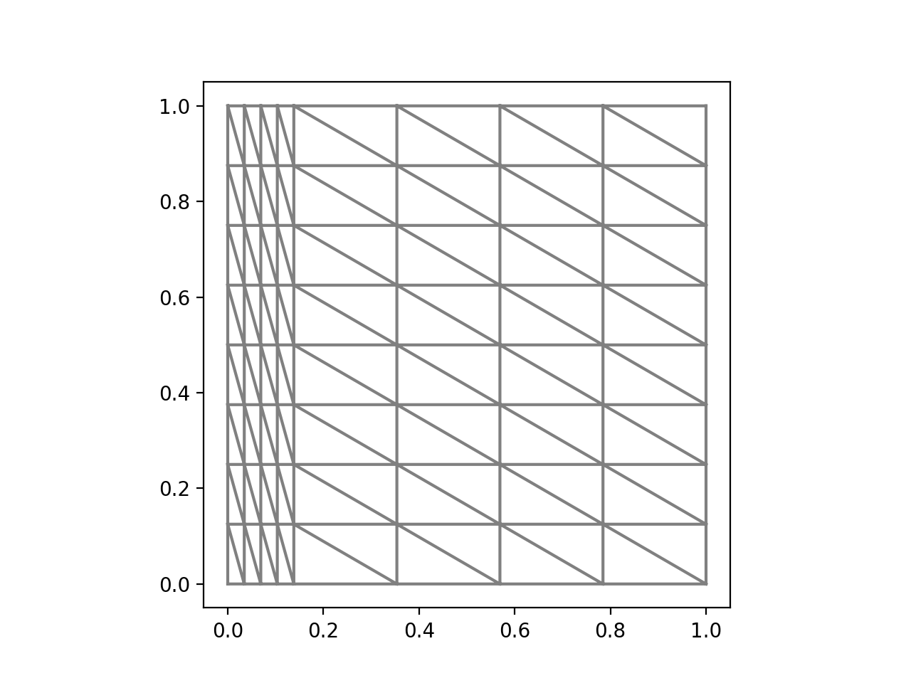
Fig. 2: Shishkin type mesh with $N=8$, $\epsilon=.01$, and $\tau=3\epsilon|\log\epsilon|$.

For this numerical experiment we compare a single barycenter and incenter refinement with $\epsilon=.01$, $\tau=3\epsilon|\log\epsilon|$, and for varying values of $N$. This results in aspect ratios of ${\varrho_{inc}}\approx 18$ and ${\varrho_{bary}}\approx 24$. We see in Fig. 3 the difference in velocity errors is negligible between the two refinement strategies. However, we see in Fig. 4 there is a small, but noticeable improvement in the pressure error when the incenter refinement is used.

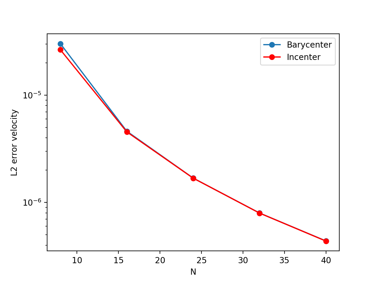
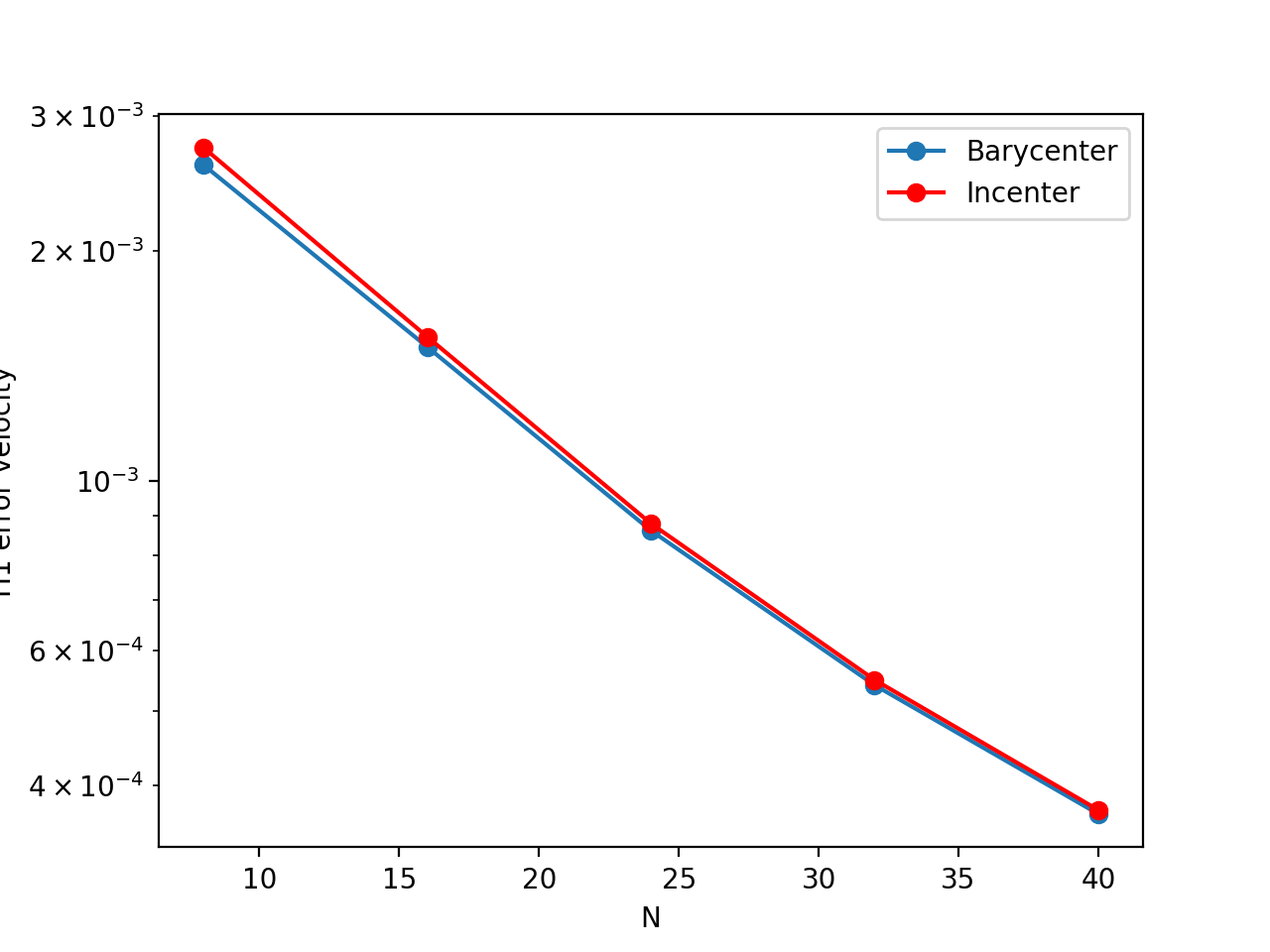
Fig. 3: Comparison of $L^{2}$ velocity error (left) and $H^{1}$ error (right) for incenter versus barycenter refinement.

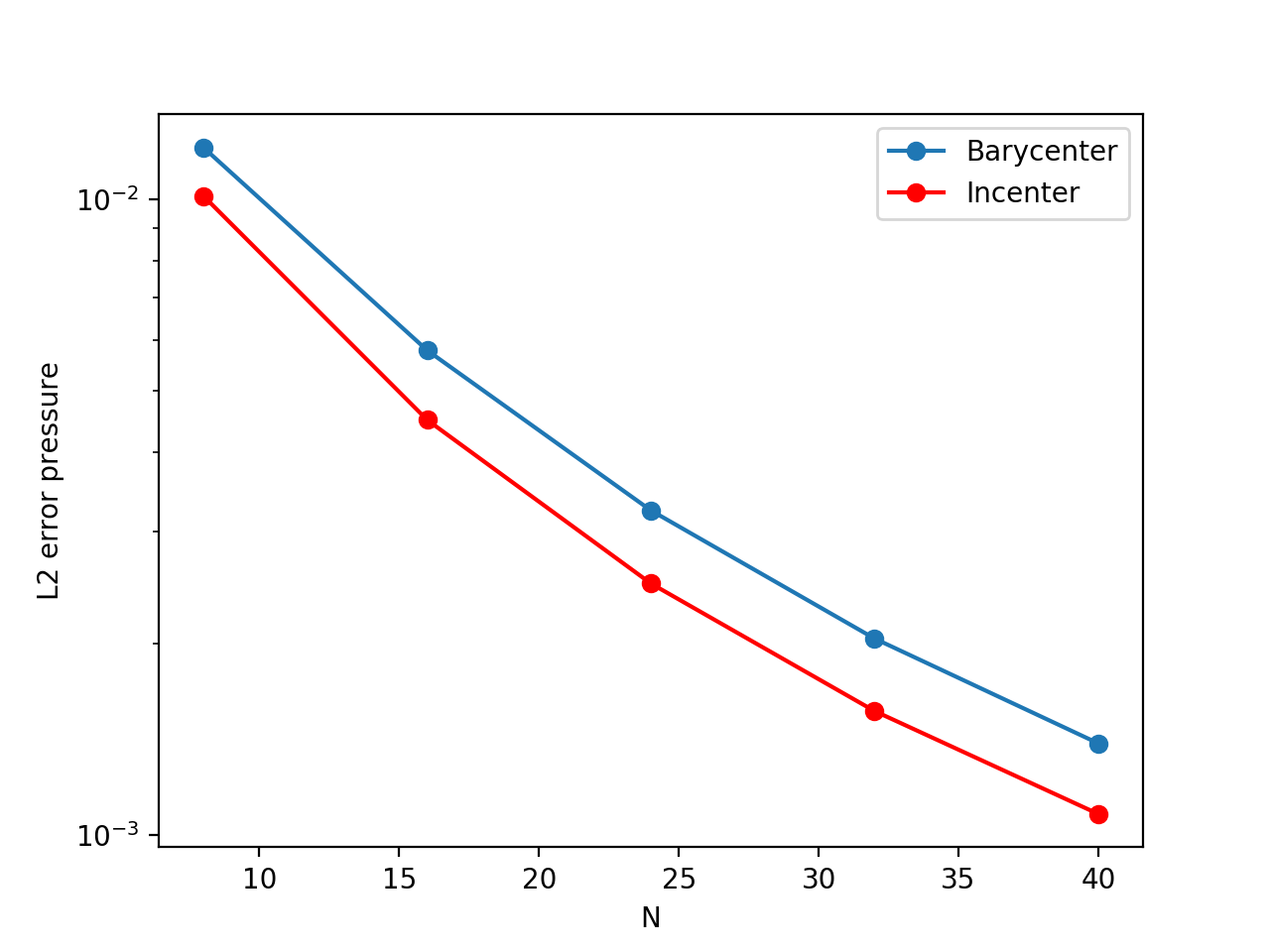
Fig. 4: Comparison of $L^{2}$ pressure error for incenter versus barycenter refinement.

Appendix A Proof of Lemma 12

Proof.

First, we may assume that $\delta<\frac{\pi}{3}.$

We will use the same notation for edges and vertices as in Section 2, in particular preserving the ordering of side lengths.

Define $t_{1}$ to be the unit vector along $e_{1}$, and $t_{2}$ to be the unit vector along $e_{2}.$ That is, $t_{1}=\frac{z_{2}-z_{3}}{h_{1}},t_{2}=\frac{z_{1}-z_{3}}{h_{2}}$. Then, let $A$ have columns $t_{1},t_{2}.$ Let $b=z_{3}.$ Then, the affine map $A\tilde{x}+b$ maps $\tilde{T}$ onto $T.$

It is clear that as each entry in $A$ is bounded above by 1 as the columns are unit vectors. Thus $\|A\|\leq 2$ and $\|adj(A)\|\leq 2,$ giving us $\|A^{-1}\|\leq\frac{2}{|det(A)|}.$

It is well known that $|det(A)|$ is the area of the parallelogram formed by the vectors $t_{1}$ and $t_{2}.$ We then have the formula

$$|det(A)|=|t_{1}||t_{2}|\sin{\alpha_{3}}=\sin{\alpha_{3}}$$

As $\alpha_{3}\in[\frac{\pi}{3},\pi-\delta],$ $\sin{\alpha_{3}}\geq\sin{\delta}$, and $\|A^{-1}\|\leq\frac{2}{\sin{\delta}}=C(\delta).$ ∎

Appendix B Proof of Lemma 14

We denote by $\tilde{F}:\hat{T}\to\tilde{T}$ the affine mapping given by

$$\tilde{F}(\hat{x})=\begin{pmatrix}h_{1}&0\\ 0&h_{2}\end{pmatrix}.$$

For $\tilde{\bm{v}}\in\bm{\EuScript{P}}_{1}(\tilde{T})$, let $\hat{\bm{v}}\in\bm{\EuScript{P}}_{1}(\hat{T})$ be given via the Piola transform

$$\tilde{\bm{v}}(\tilde{x})=\frac{1}{\det(D\tilde{F})}D\tilde{F}\hat{\bm{v}}(\hat{x})=\begin{pmatrix}h_{2}^{-1}\hat{v}_{1}(\hat{x})\\ h_{1}^{-1}\hat{v}_{2}(\hat{x})\end{pmatrix},\qquad\tilde{x}=\tilde{F}(\hat{x}).$$ (13)

Proof.

Let $\hat{\bm{v}}\in\bm{\EuScript{P}}_{1}(\hat{T})$ be defined by (13). The Brezzi-Douglas-Marini DOFs and equivalence of norms yields

$$\|\hat{\bm{v}}\|^{2}\leq C\sum_{i=1}^{3}\|\hat{\bm{v}}\cdot\hat{\bm{n}}_{i}\|_{L^{2}(\hat{e}_{i})}^{2}$$

for any norm $\|\cdot\|$ on $\bm{\EuScript{P}}_{1}(\hat{T})$. Using the identity $\hat{\bm{v}}\cdot\hat{\bm{n}}_{i}(\hat{x})=(h_{i}/|\hat{e}_{i}|)({\bm{v}}\cdot\bm{n}_{i})(x)$, we have, by a change of variables,

$$\|\hat{\bm{v}}\|^{2} \leq C\sum_{i=1}^{3}h_{i}\|{\bm{v}}\cdot\bm{n}_{i}\|_{L^{2}(e_{i})}^{2}.$$

Furthermore, by the chain rule

$$\nabla{\bm{v}}(x) =\frac{1}{\det(D\tilde{F})}D\tilde{F}\hat{\nabla}\hat{\bm{v}}(\hat{x})(D\tilde{F})^{-1}=\frac{1}{h_{1}h_{2}}\begin{pmatrix}\frac{{\partial}\hat{v}_{1}}{{\partial}\hat{x}_{1}}&\frac{h_{1}}{h_{2}}\frac{{\partial}\hat{v}_{1}}{{\partial}\hat{x}_{2}}\\ \frac{h_{2}}{h_{1}}\frac{{\partial}\hat{v}_{2}}{{\partial}\hat{x}_{1}}&\frac{{\partial}\hat{v}_{2}}{{\partial}\hat{x}_{2}}.\end{pmatrix}$$

Therefore,

$$\|\nabla{\bm{v}}\|_{L^{2}(\tilde{T})}^{2} \leq 2|\tilde{T}|(h_{1}h_{2})^{-2}\max\{\frac{h_{1}}{h_{2}},\frac{h_{2}}{h_{1}}\}\|\hat{\nabla}\hat{\bm{v}}\|_{L^{2}(\hat{T})}^{2}$$

$$=(h_{1}h_{2})^{-1}\varrho\|\hat{\nabla}\hat{\bm{v}}\|_{L^{2}(\hat{T})}^{2}$$

$$\leq C|\tilde{T}|^{-1}\varrho\sum_{i=1}^{3}k_{i}\|{\bm{v}}\cdot\bm{n}_{i}\|_{L^{2}(e_{i})}^{2}.$$

We also have

$$\|{\bm{v}}\|_{L^{\infty}(\tilde{T})}^{2}=\max\{h_{2}^{-2},h_{1}^{-2}\}\|\hat{\bm{v}}\|_{L^{\infty}(\hat{T})}^{2}\leq C|\tilde{T}|^{-1}\varrho\sum_{i=1}^{3}h_{i}\|{\bm{v}}\cdot\bm{n}\|_{L^{2}(e_{i})}^{2}.$$

∎

B.1 Proof of Lemma 15

Proof.

We have

$$k_{i}\|q\|_{L^{2}(e_{i})}^{2}\leq h_{i}k_{i}\|q\|_{L^{\infty}(e_{i})}^{2}\leq h_{i}k_{i}\|q\|_{L^{\infty}(K_{i})}^{2}.$$

Therefore by standard scaling,

$$k_{i}\|q\|_{L^{2}(e_{i})}^{2}\leq Ch_{i}k_{i}|K_{i}|^{-1}\|q\|_{L^{2}(K_{i})}^{2}\leq C\|q\|_{L^{2}(K_{i})}^{2}.$$

∎

References

• [1] Travis M. A., T. A. Manteuffel, and Steve McCormick. A robust multilevel approach for minimizing $\mathbb{H}({\rm div})$-dominated functionals in an $\mathbb{H}^{1}$-conforming finite element space. Numer. Linear Algebra Appl., 11(2-3):115–140, 2004.
• [2] G. Acota, T. Apel, R. G. Durán, and A. L. Lombardi. Error estimates for Raviart-Thomas interpolation of any order on anisotropic tetrahedra. Mathematics of Computation, 80(273):141–163, 2011.
• [3] Naveed Ahmed, Alexander Linke, and Christian Merdon. Towards pressure-robust mixed methods for the incompressible Navier-Stokes equations. Comput. Methods Appl. Math., 18(3):353–372, 2018.
• [4] M. Ainsworth, G. R. Barrenechea, and A. Wachtel. Stabilization of high aspect ratio mixed finite elements for incompressible flow. SIAM Journal on Numerical Analysis, 53(2):1107–1120, 2015.
• [5] T. Apel and V. Kempf. Brezzi–Douglas–Marini interpolation of any order on anisotropic triangles and tetrahedra. SIAM Journal on Numerical Analysis, 58(3):1696–1718, 2020.
• [6] T. Apel, V. Kempf, A. Linke, and C. Merdon. A nonconforming pressure-robust finite element method for the Stokes equations on anisotropic meshes. IMA Journal of Numerical Analysis, 01 2021. draa097.
• [7] T. Apel and S. Nicaise. The inf-sup condition for low order elements on anisotropic meshes. Calcolo, 41:89–113, 2004.
• [8] T. Apel, S. Nicaise, and J. Schöberl. Crouzeix-Raviart type finite elements on anisotropic meshes. Numer. Math., 89(2):193–223, 2001.
• [9] D. N. Arnold and J. Qin. Quadratic velocity/linear pressure Stokes elements. In Advances in Computer Methods for Partial Differential Equations VII, pages 28–34. IMACS, 1992.
• [10] G. R. Barrenechea and A. Wachtel. The inf-sup stability of the lowest order Taylor–Hood pair on affine anisotropic meshes. IMA Journal of Numerical Analysis, 40(4):2377–2398, 07 2019.
• [11] M. Akbas Belenli, L. G. Rebholz, and F. Tone. A note on the importance of mass conservation in long-time stability of Navier–Stokes simulations using finite elements. Applied Mathematics Letters, 45:98–102, 2015.
• [12] C. Bernardi and G. Raugel. Analysis of some finite elements for the Stokes problem. Mathematics of Computation, 44(169):71–79, 1985.
• [13] B. Boffi, R. Brezzi, L.F. Demkowicz, R.G. Durán, R.S. Falk, and M. Fortin. Mixed finite elements, compatibility conditions, and applications. Lectures given at the C.I.M.E. Summer School held in Cetraro, June 26–July 1, 2006, 44(169):71–79, 2008.
• [14] C. Brennecke, A. Linke, C. Merdon, and J. Schöberl. Optimal and pressure-independent $L^{2}$ velocity error estimates for a modified Crouzeix-Raviart Stokes element with BDM reconstructions. J. Comput. Math., 33(2):191–208, 2015.
• [15] A. Buffa, C. de Falco, and G. Sangalli. IsoGeometric Analysis: stable elements for the 2D Stokes equation. Internat. J. Numer. Methods Fluids, 65(11-12):1407–1422, 2011.
• [16] B. Cockburn, G. Kanschat, and D. Schotzau. A locally conservative LDG method for the incompressible Navier-Stokes equations. Math. Comp., 74(251):1067–1095, 2005.
• [17] V. DeCaria and M. Schneier. An embedded variable step imex scheme for the incompressible Navier–Stokes equations. Computer Methods in Applied Mechanics and Engineering, 376:113661, 2021.
• [18] R. S. Falk and M. Neilan. Stokes complexes and the construction of stable finite elements with pointwise mass conservation. SIAM J. Numer. Anal., 51(2):1308–1326, 2013.
• [19] P. E. Farrell, L. Mitchell, L. Ridgway Scott, and F. Wechsung. A Reynolds-robust preconditioner for the Scott-Vogelius discretization of the stationary incompressible Navier-Stokes equations. The SMAI journal of computational mathematics, 7:75–96, 2021.
• [20] J. Guzmán, A. Lischke, and M. Neilan. Exact sequences on Powell-Sabin splits. Calcolo, 57(2):Paper No. 13, 25, 2020.
• [21] J. Guzmán and M. Neilan. Conforming and divergence-free Stokes elements on general triangular meshes. Math. Comp., 83(285):15–36, 2014.
• [22] J. Guzmán and M. Neilan. Inf-sup stable finite elements on barycentric refinements producing divergence–free approximations in arbitrary dimensions. SIAM Journal on Numerical Analysis, 56(5):2826–2844, 2018.
• [23] V. John, P. Knobloch, and J. Novo. Finite elements for scalar convection-dominated equations and incompressible flow problems: a never ending story? Computing and Visualization in Science, 19:47–63, 2018.
• [24] V. John, A. Linke, C. Merdon, M. Neilan, and L. G. Rebholz. On the divergence constraint in mixed finite element methods for incompressible flows. SIAM Rev., 59(3):492–544, 2017.
• [25] C. Kreuzer and P. Zanotti. Quasi-optimal and pressure-robust discretizations of the Stokes equations by new augmented Lagrangian formulations. IMA J. Numer. Anal., 40(4):2553–2583, 2020.
• [26] P. L. Lederer, A. Linke, C. Merdon, and J. Schöberl. Divergence-free reconstruction operators for pressure-robust Stokes discretizations with continuous pressure finite elements. SIAM J. Numer. Anal., 55(3):1291–1314, 2017.
• [27] A. Linke. On the role of the Helmholtz decomposition in mixed methods for incompressible flows and a new variational crime. Comput. Methods Appl. Mech. Engrg., 268:782–800, 2014.
• [28] A. Linke, G. Matthies, and L. Tobiska. Robust arbitrary order mixed finite element methods for the incompressible Stokes equations with pressure independent velocity errors. ESAIM Math. Model. Numer. Anal., 50(1):289–309, 2016.
• [29] A. Linke and C. Merdon. Pressure-robustness and discrete Helmholtz projectors in mixed finite element methods for the incompressible Navier-Stokes equations. Comput. Methods Appl. Mech. Engrg., 311:304–326, 2016.
• [30] A. Logg, K. Mardal, and G. Wells. Automated solution of differential equations by the finite element method: The FEniCS book, volume 84. Springer Science & Business Media, 2012.
• [31] M. Neilan. The Stokes complex: a review of exactly divergence-free finite element pairs for incompressible flows. In 75 years of mathematics of computation, volume 754 of Contemp. Math., pages 141–158. Amer. Math. Soc., [Providence], RI, [2020] ©2020.
• [32] D. Schotzau and C. Schwab. Mixed hp-fem on anisotropic meshes. Mathematical Models and Methods in Applied Sciences, 08(05):787–820, 1998.
• [33] D. Schotzau, C. Schwab, and R. Stenberg. Mixed hp-fem on anisotropic meshes II: Hanging nodes and tensor products of boundary layer meshes. Numerische Mathematik, 83:667–697, 1999.
• [34] L. R. Scott and M. Vogelius. Norm estimates for a maximal right inverse of the divergence operator in spaces of piecewise polynomials. RAIRO Modél. Math. Anal. Numér., 19(1):111–143, 1985.
• [35] R. Verfürth and P. Zanotti. A quasi-optimal Crouzeix-Raviart discretization of the Stokes equations. SIAM J. Numer. Anal., 57(3):1082–1099, 2019.
• [36] S. Zhang. A new family of stable mixed finite elements for the 3D Stokes equations. Math. Comp., 74(250):543–554, 2005.