A Two-Time-Scale Stochastic Optimization Framework with Applications in Control and Reinforcement Learning

Abstract

We study a new two-time-scale stochastic gradient method for solving optimization problems, where the gradients are computed with the aid of an auxiliary variable under samples generated by time-varying Markov random processes parameterized by the underlying optimization variable. These time-varying samples make gradient directions in our update biased and dependent, which can potentially lead to the divergence of the iterates. In our two-time-scale approach, one scale is to estimate the true gradient from these samples, which is then used to update the estimate of the optimal solution. While these two iterates are implemented simultaneously, the former is updated “faster” (using bigger step sizes) than the latter (using smaller step sizes). Our first contribution is to characterize the finite-time complexity of the proposed two-time-scale stochastic gradient method. In particular, we provide explicit formulas for the convergence rates of this method under different structural assumptions, namely, strong convexity, convexity, the Polyak-Łojasiewicz (PŁ) condition, and general non-convexity.

We apply our framework to two problems in control and reinforcement learning. First, we look at the standard online actor-critic algorithm over finite state and action spaces and derive a convergence rate of $\mathcal{O}(k^{-2/5})$, which recovers the best known rate derived specifically for this problem. Second, we study an online actor-critic algorithm for the linear-quadratic regulator and show that a convergence rate of $\mathcal{O}(k^{-2/3})$ is achieved. This is the first time such a result is known in the literature. Finally, we support our theoretical analysis with numerical simulations where the convergence rates are visualized.

1 Introduction

Online policy gradient algorithms for reinforcement learning (RL), commonly referred to as “actor-critic” algorithms, can be re-cast as optimization problems with a specific type of stochastic oracle for gradient evaluations. In this paper, we present a simple actor-critic-like algorithm solving general optimization problems with this same form, and give convergence guarantees for different types of assumed structural properties of the function being optimized. Our abstraction unifies the analysis of actor-critic methods in RL, and we show how our main results reproduce the best-known convergence rates for the general policy optimization problem and how they can be used to derive a state-of-the-art rate for the online linear-quadratic regulator (LQR) controllers.

Our optimization framework is described as follows. The overall goal is to solve the (possibly non-convex) program

$$\min_{\theta\in\mathbb{R}^{d}}~{}f(\theta),$$ (1)

where the gradient of $f$ is accessed through a stochastic oracle $H(\theta,\omega,X)$. The three arguments to $H$ are the decision variable $\theta$, an auxiliary variable $\omega\in\mathbb{R}^{r}$, and a random variable $X$ drawn over a compact sample space ${\cal X}$. For a fixed $\theta$, there is a single setting of the auxiliary variable, which we will denote $\omega^{\star}(\theta)$, such that $H$ returns an unbiased estimate of the gradient $\nabla f(\theta)$ when $X$ is drawn from a particular distribution $\mu_{\theta}$,

$$\nabla f(\theta)=\mathbb{E}_{X\sim\mu_{\theta}}[H(\theta,\omega^{\star}(\theta),X)].$$ (2)

For other settings of $\omega\neq\omega^{\star}(\theta)$ or $X$ drawn from a distribution other than $\mu_{\theta}$, $H(\theta,\omega,X)$ will be (perhaps severely) biased. The mapping from $\theta$ to the “optimal” setting of the auxiliary variable $\omega^{\star}(\theta)$ is implicit; it is determined by solving a nonlinear system of equations defined by another stochastic sampling operator $G:\mathbb{R}^{d}\times\mathbb{R}^{r}\times{\cal X}\rightarrow\mathbb{R}^{r}$. Given $\theta$, $\omega^{\star}(\theta)$ is the (we will assume unique) solution to

$$\mathbb{E}_{X\sim\mu_{\theta}}[G(\theta,\omega^{\star}(\theta),X)]=0.$$ (3)

Combining (2) and (3), solving (1) is equivalent to finding $(\theta^{\star},\omega^{\star}(\theta^{\star}))$ that satisfies

$$\left\{\begin{array}[]{ll}&\mathbb{E}_{X\sim\mu_{\theta^{\star}}}[H(\theta^{\star},\omega^{\star}(\theta^{\star}),X)]=0,\\ &\mathbb{E}_{X\sim\mu_{\theta^{\star}}}[G(\theta^{\star},\omega^{\star}(\theta^{\star}),X)]=0.\end{array}\right.$$ (6)

In the applications we are interested in, we only have indirect access to the distribution $\mu_{\theta}$. Instead of parameterizing a distribution directly, $\theta$ parameterizes a set of probability transition kernels on ${\cal X}\times{\cal X}$ through a mapping ${\cal P}:{\cal X}\times\mathbb{R}^{d}\rightarrow\text{dist}({\cal X})$. Given $\theta$ and $X$, we will assume that we can generate a sample $X^{\prime}\sim{\cal P}(\cdot|X,\theta)$ using one of these kernels. Each of these ${\cal P}(\cdot|\cdot,\theta)$ induces a different Markov chain and a different stationary distribution $\mu_{\theta}$, which is what is used in (2) and (3) above.

This problem structure is motivated by online algorithms for reinforcement learning [35, 34, 22]. In this class of problems, two of which we describe in details in Section 5, we are searching for a control policy parameterized by $\theta$ that minimizes a long term cost captured by the function $f$. The gradient for this cost depends on the value function the policy indexed by $\theta$, which is specified implicitly through the Bellman equation, the analog to (3) above. These problems often also have a mechanism for generating samples, either through experiments or simulations, that makes only implicit use of the transition kernel ${\cal P}$.

If we were able to generate independent and identically distributed (i.i.d.) samples from $\mu_{\theta}$ given any $\theta$ then a straightforward approach to solving (6) would be to use a nested-iterations approach. With $\theta$ fixed, we could sample $X\sim\mu_{\theta}$ repeatedly to (approximately) solve (3) using stochastic approximation, then with $\theta$ and $\omega^{\star}(\theta)$ fixed sample again and average over evaluations of $H$ to provide an (almost unbiased) estimate of the gradient in (2). While there is an established methodology for analyzing this type of nested loop algorithm, variants of which have appeared in the control and RL literature in [40, 39, 31], they tend to be “sample hungry” in practice. The method we will study below is truly online, updating estimates of both the auxiliary and decision variables after each sample observation. This type of update is usually favored in practice as the implementation is simpler and empirically requires fewer samples [37, 36].

An additional complication is that for a given $\theta$, actually generating samples from the induced stationary distribution $\mu_{\theta}$ is expensive and often impractical, requiring many draws using the kernels ${\cal P}$ for a burn-in period and re-starting the Markov chain many times. Our online update simply draws a single sample in every iteration $k$ according to $X_{k}\sim{\cal P}(\cdot|X_{k-1},\theta_{k})$, where $\theta_{k}$ is the decision variable iterate whose updates will be discussed in Section 2. This results in a time-varying Markov chain for $\{X_{k}\}$, which requires delicate analytical treatment. Nevertheless, we are able to show that this non-stationarity settles down over time and establish rates of convergence of the decision variable and auxiliary variable iterates.

Finally, we note that along with applications in reinforcement learning, problems that involve the types of coupled system of equations described above also appear in bi-level optimization [17] and generative adversarial models [14].

1.1 Main Contribution

The main contributions of this paper are twofold. First, we develop a new two-time-scale SGD method for solving (1) under the general stochastic oracle described above. This is an iterative algorithm that requires exactly one evaluation of $H$, one evaluation of $G$, and one query of the sampling procedure for each iteration. We then analyze the finite-time and finite-sample complexity of the proposed method under when the objective function has different types of structure, namely strong convexity, convexity, the Polyak-Lojasiewicz (PŁ) condition, and general non-convexity. For each type of function structure, we provide an explicit upper bound on the convergence rate that has been tuned to the decay rate of the step sizes. The finite-time convergence rates are summarized in Table 1, where $k$ denotes the number of algorithm iterations. Since we draw exactly one sample in every iteration of the algorithm, the sample complexity has the same order as the time complexity. The key technical challenge in our analysis is to handle the coupling between the two iterates while addressing the impacts of time-varying Markovian randomness.

Second, we demonstrate how our theoretical results apply to actor-critic algorithms for two different reinforcement learning problems. Although these are both reinforcement learning problems, they have significantly different structure; nevertheless, our framework and analysis apply easily to both cases. We start with the general finite state and action space setting using infinite-horizon average-cost. Here our analysis recovers the state-of-the-art result for online actor-critic algorithms for policy optimization. Next we describe how our general framework can also be specialized as an online natural actor-critic method for solving the classic linear-quadratic regulator (LQR) problem, providing the first known finite-sample complexity guarantee for an online algorithm for this problem. Specifically, we prove that after $k$ iterations, this method has found a control that is within ${\cal O}(k^{-2/3})$ of the optimal control in terms of the infinite-horizon average cost. Key to our analysis is exploiting the fact that the LQR problem has an objective that obeys the PŁ condition. To support our theoretical results, we provide numerical simulations that illustrate the convergence rate of our method for solving the LQR.

Table 1: Summary of Main Results - Time and Sample Complexity.
$\theta^{\star}$ is an optimal solution to (1). $\bar{\theta}_{k}$ is a weighted average of the iterates defined in (34).

Structural Property of $f$	Metric	Rate	$\alpha_{k}$, $\beta_{k}$
Strong Convexity	$\mathbb{E}[\|\theta_{k}-\theta^{\star}\|^{2}$]	${\cal O}(k^{-2/3})$	${\cal O}(k^{-1}),{\cal O}(k^{-2/3})$
Convexity	$\mathbb{E}[f(\bar{\theta}_{k})-f(\theta^{\star})]$	${\cal O}(k^{-1/4})$	${\cal O}(k^{-3/4}),{\cal O}(k^{-1/2})$
PŁ Condition	$\mathbb{E}[f(\theta_{k})-f(\theta^{\star})]$	${\cal O}(k^{-2/3})$	${\cal O}(k^{-1}),{\cal O}(k^{-2/3})$
Non-convexity	$\min_{t\leq k}\mathbb{E}[\|\nabla f(\theta_{t})\|^{2}]$	${\cal O}(k^{-2/5})$	${\cal O}(k^{-3/5}),{\cal O}(k^{-2/5})$

1.2 Related Work

Our work closely relates to the existing literature on two-time-scale stochastic approximation (SA), actor-critic algorithms in reinforcement learning, and SGD under Markovian samples. In this section, we discuss the recent progress in these three domains and point out our novelty.

First, two-time-scale stochastic approximation aims to solve a system of equations that has a similar form to (6), but often considers the setting where $\mu_{\theta}=\mu$, a fixed distribution over a statistical sample space. The convergence of the two-time-scale SA is traditionally established through the analysis of an associated ordinary differential equation (ODE) [2]. Finite-time convergence of the two-time-scale SA has been studied for both linear [23, 5, 4, 11, 16, 7, 19, 12] (when $H$ and $G$ are linear) and nonlinear settings [28, 8, 6], under both i.i.d. and Markovian samples. In addition, the analysis in the nonlinear setting is only established when $H$ and $G$ are both strongly monotone [8, 6]. The work in [17] for solving bi-level optimization problems can also be viewed as a variant of the two-time-scale SA algorithm, where the authors assume that the bias of the gradient estimate satisfies certain decay properties. Compared with these prior works, the novelty of our work is twofold. While the previous works in two-time-scale SA solve a system of equation under a fixed distribution $\mu$, we aim to solve (6) where the distribution of the samples also depends on the decision variable. This is an important generalization as many realistic problems in control and reinforcement learning can only be abstracted as (6) with $\mu_{\theta}$ being a function of the control variable. Making this generalization requires generating decision-variable-dependent samples from a Markov chain whose stationary distribution shifts over iterations, which creates additional challenges in the analysis. Furthermore, while the previous works consider linear or strongly monotone $H$, our work studies a wide range of function structures including strong convexity, convexity, PŁ condition, and general non-convexity. As we will see in Section 5.1, the fast convergence guarantee for PŁ functions is particularly interesting due to its tie to the LQR problem in stochastic control.

Second, in the RL literature actor-critic algorithms also aim to solve a problem similar to (6), where $\theta$ and $\omega^{\star}(\theta)$ are referred to as the actor and critic, respectively; see for example [21, 30, 24, 37, 36, 38]. Among these works, only [21, 36] consider an online setting similar to the one studied in this paper. In fact, the online actor-critic algorithm in RL is a special case of our framework with a non-convex objective function $f$. Our analysis recovers the state-of-the-art result in this domain [36], while being more general by removing the projection operation in the update of the critic parameter used to limit the growth of its norm.

Last but not least, we note that our paper is related to the works on stochastic algorithms under Markovian samples. In particular, [32, 9, 10, 41] study various SGD/SA algorithms under samples generated from a fixed Markov chain and show that the convergence rates are only different from that under i.i.d. samples by a log factor. The authors in [43] consider a variant of SA under stochastic samples from a time-varying Markov chain controlled by the decision variable. The algorithm in our work also updates with samples drawn from a time-varying Markov chain. However, we study two-time-scale methods while the work in [43] only consider a single-time-scale SA.

2 Two Time-scale Stochastic Gradient Descent

In this section, we present our two-time-scale SGD method (formally stated in Algorithm 1) for solving (6) under the gradient oracles discussed in Section 1.

Algorithm 1 Two Timescale Stochastic Gradient Descent

1:  Initialization: the decision variable $\theta_{0}$, auxiliary variable $\omega_{0}$, and step size sequences $\{\alpha_{k}\}$ for the decision variable update, $\{\beta_{k}\}$ for the auxiliary variable update

2:  Observe a initial sample $X_{0}$

3:  for $k=1,2,3,...$ do

4:     Decision variable update:

$$\theta_{k+1} =\theta_{k}-\alpha_{k}H(\theta_{k},\omega_{k},X_{k})$$ (7)

5:     Auxiliary variable update:

$$\omega_{k+1}=\omega_{k}-\beta_{k}G(\theta_{k+1},\omega_{k},X_{k})$$ (8)

6:     Draw sample

$$X_{k+1}\sim{\cal P}(\cdot\mid X_{k},\theta_{k+1})$$ (9)

7:  end for

In Algorithm 1, $\theta_{k}$ and $\omega_{k}$ are estimates of $\theta^{\star}$ and $\omega^{\star}(\theta^{\star})$. The random variables $\{X_{k}\}$ are generated by a Markov process parameterized by $\{\theta_{k}\}$ under the transition kernel ${\cal P}$, i.e.,

$$X_{0}\stackrel{{\scriptstyle\theta_{1}}}{{\longrightarrow}}X_{1}\stackrel{{\scriptstyle\theta_{2}}}{{\longrightarrow}}X_{2}\stackrel{{\scriptstyle\theta_{3}}}{{\longrightarrow}}\cdots\stackrel{{\scriptstyle\theta_{k-1}}}{{\longrightarrow}}X_{k-1}\stackrel{{\scriptstyle\theta_{k}}}{{\longrightarrow}}X_{k}.$$ (10)

As $\theta_{k}$ changes at every iteration, so do the dynamics of this Markov process that generates the data. At finite time step $k$, $X_{k}$ is in general not an i.i.d. sample from the stationary distribution $\mu_{\theta_{k}}$, implying that $H(\theta_{k},\omega_{k},X_{k})$ employed in the update (7) is not an unbiased estimate of $\nabla f(\theta_{k})$ even if $\omega_{k}$ were to track $\omega^{\star}(\theta_{k})$ perfectly. This sample bias, along with the error in the difference between $\omega_{k}$ and $\omega^{\star}(\theta_{k})$, affects the variables $\theta_{k+1}$ and $\omega_{k+1}$ of the next iteration and accumulates inaccuracy over time which we need to control.

The updates use two different step sizes, $\alpha_{k}$ and $\beta_{k}$. We choose $\alpha_{k}\ll\beta_{k}$ as a way to approximate, very roughly, the nested-loop algorithm that runs multiple auxiliary variable updates for each decision variable update. Many small critic updates get replace with a single large one. In other words, the auxiliary variable $\omega_{k}$ is updated at a faster time scale (larger step size) as compared to $\theta_{k}$ (smaller step size).

The ratio $\beta_{k}/\alpha_{k}$ can be interpreted as the time-scale difference. We will see that this ratio needs to be carefully selected based on the structural properties of the function $f$ for the algorithm to achieve the best possible convergence. Table  1 provides a brief summary of our main theoretical results, which characterizes the finite-time complexity of Algorithm 1 and the corresponding optimal choice of step sizes under different function structures.

3 Technical Assumptions

In this section, we present the main technical assumptions important in our later analysis. We first consider the smoothness assumption of $H$ and $G$ and the boundedness condition $H$ as below.

Assumption 1

There exists a constant $L>0$ such that for all $\theta_{1},\theta_{2}\in\mathbb{R}^{d},$ $\omega_{1},\omega_{2}\in\mathbb{R}^{r}$, and $X\in{\cal X}$

$$\left\|H(\theta_{1},\omega_{1},X)-H(\theta_{2},\omega_{2},X)\right\|\leq L\left(\|\theta_{1}-\theta_{2}\|+\|\omega_{1}-\omega_{2}\|\right),$$

$$\left\|G(\theta_{1},\omega_{1},X)-G(\theta_{2},\omega_{2},X)\right\|\leq L\left(\|\theta_{1}-\theta_{2}\|+\|\omega_{1}-\omega_{2}\|\right).$$ (11)

In addition, there exits a constant $B>0$ such that

$$\|H(\theta,\omega,X)\|\leq B,\quad\forall\theta\in\mathbb{R}^{d},\omega\in\mathbb{R}^{r},X\in{\cal X}.$$ (12)

We also assume the smoothness of the objective function $f$.

Assumption 2

There exists a constant $L>0$ such that for all $\theta_{1},\theta_{2}\in\mathbb{R}^{d}$

$$\left\|\nabla f(\theta_{1})-\nabla f(\theta_{2})\right\|\leq L\|\theta_{1}-\theta_{2}\|.$$ (13)

Assumptions 1 and 2 are common in the literature of stochastic approximation [3, 6] and hold in the context of actor-critic methods, which we will verify in Section 5. Next, we assume that the operator $G$ is strongly monotone in expectation at its root (which we have assumed is unique).

Assumption 3

There exists a constant $\lambda_{G}>0$ such that

$$\left\langle\mathbb{E}_{X\sim\mu_{\theta}}[G(\theta,\omega,X)],\omega-\omega^{\star}(\theta)\right\rangle\leq-\lambda_{G}\|\omega-\omega^{\star}(\theta)\|^{2},\quad\forall\theta\in\mathbb{R}^{d},\omega\in\mathbb{R}^{r}.$$

This assumption is often made in the existing literature on two-time-scale stochastic approximation [17, 6] and is a sufficient condition to guarantee the fast convergence of the auxiliary variable iterate. We will verify that Assumption 3 (or an equivalent contractive condition) holds in the actor-critic methods discussed in Section 5.

In addition, we assume that the solution $\omega^{\star}(\cdot)$ is $L$-Lipschitz continuous with respect to $\theta$ as follows.

Assumption 4

There exists a constant $L,B>0$ such that

$$\left\|\omega^{\star}(\theta_{1})-\omega^{\star}(\theta_{2})\right\|\leq L\|\theta_{1}-\theta_{2}\|,\quad\forall\theta_{1},\theta_{2}\in\mathbb{R}^{d}$$

$$\hskip 50.0pt\left\|\omega^{\star}(\theta)\right\|\leq B,\quad\forall\theta\in\mathbb{R}^{d}.$$

Note that we use the same constants $L$ and $B$ in the three assumptions mentioned above for the convenience of notation.

Given two probability distributions $\mu_{1}$ and $\mu_{2}$ over the space ${\cal X}$, their total variation distance is defined as

$$d_{\text{TV}}(\mu_{1},\mu_{2})=\frac{1}{2}\sup_{\nu:{\cal X}\rightarrow[-1,1]}\left|\int\nu d\mu_{1}-\int\nu d\mu_{2}\right|.$$ (14)

The definition of the mixing time of a Markov chain $\{X_{k}\}$ is given as follows.

Definition 1

Consider the Markov chain $\{X_{k}^{\theta}\}$ generated according to $X_{k}^{\theta}\sim{\cal P}(\cdot\mid X_{k-1}^{\theta},\theta)$, and let $\mu_{\theta}$ be its stationary distribution. For any $\alpha>0$, the mixing time of the chain $\{X_{k}^{\theta}\}$ corresponding to $\alpha$ is defined as

$$\tau_{\theta}(\alpha)=\min\{k\geq 0:\sup_{X\in{\cal X}}d_{\text{TV}}(P(X_{k}^{\theta}=\cdot\mid X_{0}^{\theta}=X),\mu_{\theta}(\cdot))\leq\alpha\}.$$

The mixing time $\tau_{\theta}(\alpha)$ essentially measures the time needed for the Markov chain $\{X_{k}^{\theta}\}$ to approach its stationary distribution [25]. We next consider the following important assumption that guarantees that the Markov chain induced by any static $\theta$ “mixes” geometrically.

Assumption 5

Given any $\theta$, the Markov chain $\{X_{k}\}$ generated by ${\cal P}(\cdot\mid\cdot,\theta)$ has a unique stationary distribution $\mu_{\theta}$ and is uniformly geometrically ergodic. In other words, there exist constants $C_{0}\geq 1$ and $\rho\in(0,1)$ independent of $\theta$ such that

$$\sup_{X\in{\cal X}}d_{\text{TV}}(P(X_{k}=\cdot\,|X_{0}=X,\,\theta),\mu_{\theta}(\cdot))\leq C_{0}\rho^{k}\text{ for all }\theta\in\mathbb{R}^{d}\text{~{}and }k\geq 0.$$

This assumption implies that there exists a positive constant $C$ depending only on $\rho$ and $C_{0}$ such that

$$\tau_{\theta}(\alpha)\leq C\log\left(1/\alpha\right),$$ (15)

for all $\theta$. In the rest of the paper, we denote

$$\tau(\alpha)\triangleq\sup_{\theta\in\mathbb{R}^{d}}\tau_{\theta}(\alpha)\leq C\log\left(1/\alpha\right).$$

Assumption 5 is again fairly standard in the analysis of Markov SGD and reinforcement learning algorithms [3, 43, 41].

Finally, we consider the following assumption on the ensemble of transition kernels:

Assumption 6

Given $\theta,\hat{\theta}\in\mathbb{R}^{d}$ and $X,\hat{X}\in{\cal X}$, let $X^{\prime}\sim{\cal P}(\cdot\mid X,\theta)$ and $\hat{X}^{\prime}\sim{\cal P}(\cdot\mid\hat{X},\theta^{\prime})$. Then there exists a constant $L>0$

$$d_{\text{TV}}(P(X^{\prime}=\cdot),P(\hat{X}^{\prime}=\cdot))\leq d_{\text{TV}}(P(X=\cdot),P(\hat{X}=\cdot))+L\|\theta-\hat{\theta}\|.$$ (16)

In addition, we assume that

$$d_{\text{TV}}(\mu_{\theta},\mu_{\hat{\theta}})\leq L\|\theta-\hat{\theta}\|.$$ (17)

This assumption amounts to a regularity condition on the transition probability matrix ${\cal P}(\cdot\mid\cdot\theta)$ as a function of $\theta$, and has been shown to hold before in the context of actor-critic methods in reinforcement learning (see, for example, [36, Lemma A1]). We also use the same constant $L$ as in Assumptions 1–4 without loss of generality. We define

$$D=\max\{L+\max_{X\in{\cal X}}\|G(0,0,X)\|,\|\omega^{*}(0)\|\},$$ (18)

which is a finite constant since ${\cal X}$ is compact. Finally, we assume that the optimal solution set $\Theta^{\star}=\{\theta^{\star}:f(\theta^{\star})\leq f(\theta)\,\forall\theta\in\mathbb{R}^{d}\}$ is non-empty.

4 Main Results

In this section, we present the main results of this paper, which are the finite-time convergence of Algorithm 1 under different objective functions, namely, strong convexity, convexity, PŁ condition, and general non-convexity. We start by briefly explaining the main technical challenges and the role of our technical assumptions in analyzing two-time-scale SGD under time-varying Markovian samples in Section 4.1. In Section 4.2, we introduce an important lemma that performs Lyapunov analysis on a coupled dynamical system of two inequalities. This lemma is a unified tool to analyze our algorithm under different function structures and can be of independent interest in the study of other multiple-time-scale coupled dynamical systems. Finally, we present our main theorems in Section 4.3 on the convergence of the decision variable.

4.1 Technical Challenges

The main technical challenge in analyzing Algorithm 1 is to handle the coupling between $\theta$, $\omega$, and the time-varying Markovian samples simultaneously. It also worth noting that the Markovian samples affect the current update of $\theta$, which induces the Markov chain used to generate the future samples. To illustrate the complications involved, we quickly look at how we might show $\|\theta_{k}-\theta^{\star}\|^{2}\rightarrow 0$ in the case where $f$ is strongly convex. Using the update rule (7), we have the following recursion on $\|\theta_{k}-\theta^{\star}\|^{2}$:

$$\|\theta_{k+1}-\theta^{\star}\|^{2}=\|\theta_{k}-\theta^{\star}\|^{2}-2\alpha_{k}\langle\theta_{k}-\theta^{\star},H(\theta_{k},\omega_{k},X_{k})\rangle+\alpha_{k}^{2}\|H(\theta_{k},\omega_{k},X_{k})\|^{2}$$

$$=\|\theta_{k}-\theta^{\star}\|^{2}-2\alpha_{k}\Big{\langle}\theta_{k}-\theta^{\star},\mathbb{E}_{\hat{X}\sim\mu_{\theta_{k}}}[H(\theta_{k},\omega^{\star}(\theta_{k}),\hat{X})]\Big{\rangle}+\alpha_{k}^{2}\|H(\theta_{k},\omega_{k},X_{k})\|^{2}$$

$$\quad-2\alpha_{k}\underbrace{\Big{\langle}\theta_{k}-\theta^{\star},H(\theta_{k},\omega^{\star}(\theta_{k}),X_{k})-\mathbb{E}_{\hat{X}\sim\mu_{\theta_{k}}}[H(\theta_{k},\omega^{\star}(\theta_{k}),\hat{X})]\Big{\rangle}}_{T_{1}}$$

$$\quad-2\alpha_{k}\underbrace{\langle\theta_{k}-\theta^{\star},H(\theta_{k},\omega_{k},X_{k})-H(\theta_{k},\omega^{\star}(\theta_{k}),X_{k})\rangle}_{T_{2}}$$

$$\approx(1-2\lambda_{G}\alpha_{k}+\alpha_{k}^{2})\|\theta_{k}-\theta^{\star}\|^{2}+T_{1}+T_{2},$$

where in the last equality we use $\nabla f(\theta_{k})=\mathbb{E}_{\hat{X}\sim\mu_{\theta_{k}}}[H(\theta_{k},\omega^{\star}(\theta_{k}),\hat{X})]$ (cf. (2)) and the strong convexity of $f$. We refer to $T_{1}$ as the time-varying Markovian noise and $T_{2}$ as the bias due to the inaccurate auxiliary variable. If the samples were i.i.d. and the auxiliary variables were always solved perfectly, we would have $\mathbb{E}[T_{1}]=\mathbb{E}[T_{2}]=0$, reducing the problem to the one studied in the standard SGD. Our focus in this work is to investigate how $T_{1}$ and $T_{2}$ can be properly controlled in the presence of the Markovian noise and inexact auxiliary variables.

First, to analyze $T_{1}$ we will use both Assumptions 5 and 6. On the one hand, Assumption 5 implies that the Markov chain induced by each $\theta_{k}$ has geometric mixing time. On the other hand, as $\theta_{k}$ evolves over time we have a sequence of time-varying Markov chains. By using Assumption 6, we are able to show that the size of errors caused by any two Markov chains associated with any two iterates $\theta$ can be bounded by the distance of these iterates. In a sense, using these two assumptions we will show that the bias of the gradient samples decays to zero.

Second, to study the error caused by $T_{2}$, we will use the Lipschitz continuity of $H$ so that the size of $T_{1}$ can be bounded by both $\|\theta_{k}-\theta^{\star}\|^{2}$ and $\|\omega_{k}-\omega^{\star}(\theta_{k})\|^{2}$. This together with our results in bounding $T_{1}$ studied above gives

$$\mathbb{E}[\|\theta_{k+1}-\theta^{\star}\|^{2}]\approx(1-{\cal O}(\alpha_{k}))\mathbb{E}[\|\theta_{k}-\theta^{\star}\|^{2}]+{\cal O}(\alpha_{k})\mathbb{E}[\|\omega_{k}-\omega^{\star}(\theta_{k})\|^{2}]+\text{noise},$$

where $\|\omega_{k}-\omega^{\star}(\theta_{k})\|^{2}$ will be analyzed by using Assumption 3. Specifically, we can derive

$$\mathbb{E}[\|\omega_{k+1}-\omega^{\star}(\theta_{k+1})\|^{2}] \leq(1-{\cal O}(\beta_{k}))\mathbb{E}[\|\omega_{k}-\omega^{\star}(\theta_{k})\|^{2}]+{\cal O}(\beta_{k})\mathbb{E}\left[\|\theta_{k}\|^{2}\right]+\text{noise},$$

where the details of this analysis will be presented in Proposition 1 later. As mentioned above, the update of the auxiliary variable $\omega_{k}$ occurs at a faster time scale, i.e. $\alpha_{k}\ll\beta_{k}$, in order to provide a more accurate gradient for the update of $\theta_{k}$. The two inequalities above form a coupled dynamical system that evolves under two different rates. To characterize the coupling of the two iterates and analyze the finite-time complexity, we consider the following Lyapunov function

$$V(\theta_{k},\omega_{k})=\mathbb{E}[\|\theta_{k}-\theta^{\star}\|^{2}]+\frac{\alpha_{k}}{\beta_{k}}\mathbb{E}[\|\omega_{k}-\omega^{\star}(\theta_{k})\|^{2}].$$

We derive the finite-time convergence rate of $V(\theta_{k},\omega_{k})$ to 0, which immediately translates convergence rates for $\mathbb{E}[\|\theta_{k}-\theta^{\star}\|^{2}]$ and $\mathbb{E}[\|\omega_{k}-\omega^{\star}(\theta_{k})\|^{2}]$.

4.2 Two-Time-Scale Lemma

Although we analyze the performance of our algorithm for different types of objective functions and using different convergence metrics, we will see that these analyses eventually reduce to the study of two coupled inequalities. The dynamics of these two inequalities happen on different time scales determined by the two step sizes used in our algorithm. In this section we present a general result, which we call the two-time-scale lemma, that characterizes the behavior of these coupled inequalities. This lemma gives us a tool for a unified analysis for different types of objectives $f$, and may be of further interest to the study of the finite-time performance of multiple-time-scale dynamical systems apart from those considered in this paper. The proof of Lemma 1 is given in Appendix B.1.

Lemma 1

Let $\{a_{k},\,b_{k},\,c_{k},\,d_{k},\,e_{k},\,f_{k}\}$ be non-negative sequences that satisfy

$$\frac{a_{k+1}}{d_{k+1}}\leq\frac{a_{k}}{d_{k}}<1,\quad\text{for all }k\geq 0.$$ (19)

Let $\{x_{k},y_{k}\}$ be two non-negative sequences. We consider the following two settings on the dynamics of $x_{k},y_{k}$:

1. Suppose that $x_{k},y_{k}$ satisfy the following coupled dynamics

   $$x_{k+1}\leq(1-a_{k})x_{k}+b_{k}y_{k}+c_{k},$$ (20)

   $$y_{k+1}\leq(1-d_{k})y_{k}+e_{k}x_{k}+f_{k}.$$ (21)

   In addition, assume that there exists a constant $A\in\mathbb{R}$ such that

   $$Aa_{k}-b_{k}-\frac{Aa_{k}^{2}}{d_{k}}\geq 0\qquad\text{and}\qquad\frac{Aa_{k}e_{k}}{d_{k}}\leq\frac{a_{k}}{2},\quad\text{for all }k\geq 0.$$ (22)

   Then we have for all $0\leq\tau\leq k$

   $$x_{k} \leq(x_{\tau}+\frac{Aa_{\tau}}{d_{\tau}}y_{\tau})\prod_{t=\tau}^{k-1}(1-\frac{a_{t}}{2})+\sum_{\ell=\tau}^{k-1}\left(c_{\ell}+\frac{Aa_{\ell}f_{\ell}}{d_{\ell}}\right)\prod_{t=\ell+1}^{k-1}(1-\frac{a_{t}}{2}).$$

2. Suppose that $\{x_{k},y_{k}\}$ satisfy the following coupled dynamics

   $$x_{k+1}\leq(1+a_{k})x_{k}+b_{k}y_{k}+c_{k},$$ (23)

   $$y_{k+1}\leq(1-d_{k})y_{k}+e_{k}x_{k}+f_{k}.$$ (24)

   $\{u_{k}\}$ is a non-negative sequence that satisfies

   $$u_{k}\leq(1+a_{k})x_{k}-x_{k+1}+b_{k}y_{k}+c_{k},$$ (25)

   then we have for any $0\leq\tau\leq k$

   $$\sum_{t=\tau}^{k}u_{t}\leq\left(1+\sum_{t=\tau}^{k}(a_{t}+\frac{b_{t}e_{t}}{d_{t}})e^{\sum_{t=\tau}^{k}(a_{t}+\frac{b_{t}e_{t}}{d_{t}})}\right)\left(x_{\tau}+\frac{b_{\tau}y_{\tau}}{d_{\tau}}+\sum_{t=\tau}^{k}(c_{t}+\frac{b_{t}f_{t}}{d_{t}})\right).$$

Lemma 1 studies the behavior of the two interacting sequences $\{x_{k}\}$ and $\{y_{k}\}$ that have generic structure. We will show in our later analysis that properly selected convergence metrics on $\theta_{k}$ and $\omega_{k}$ evolve as $x_{k}$ and $y_{k}$ above, respectively, according to either (20)-(21) or (23)-(24) under different structures of $f$, while the sequences $\{a_{k},\,b_{k},\,c_{k},\,d_{k},\,e_{k},\,f_{k}\}$ are ratios and products of the step sizes $\{\alpha_{k}\}$ and $\{\beta_{k}\}$.

4.3 Finite-Time Complexity of Two-Time-Scale SGD

In this subsection, we present the main results studied in this paper, which is the finite-time complexity of Algorithm 1. We analyze the convergence rates of the two-time-scale SGD algorithm under four structural properties of the function $f$, namely, strong convexity, convexity, non-convexity with the PŁ condition, and general non-convexity. Our results are derived under the assumptions introduced in Section 3, which we assume always hold in the rest of this paper. The analysis of these results will be presented in Section 7.

The convergence of Algorithm 1 relies on $\alpha_{k},\beta_{k}\rightarrow 0$ with reasonable rates. As mentioned in Section 2, $\alpha_{k}$ needs to be much smaller than $\beta_{k}$ to approximate the nested-loop algorithm where multiples auxiliary variable updates are performed for every decision variable update. Therefore, we consider the following choices of step sizes

$$\alpha_{k}=\frac{\alpha_{0}}{(k+1)^{a}},\quad\beta_{k}=\frac{\beta_{0}}{(k+1)^{b}},\quad\forall k\geq 0,$$ (26)

where $a,b,\alpha_{0},\beta_{0}$ are some constants satisfying $0<b\leq a\leq 1$ and $0<\alpha_{0}\leq\beta_{0}$. Given any $\alpha_{k}$, recall that $\tau(\alpha_{k})$ is the mixing time corresponding to $\alpha_{k}$ for the Markov chain induced by $\{\theta_{k}\}$ defined in Definition 1. In the sequel, for convenience we use a shorthand notation $\tau_{k}$ to denote this mixing time

$$\tau_{k}\triangleq\tau(\alpha_{k}).$$ (27)

Since $\tau_{k}\leq C\log((k+1)^{a}/\alpha_{0})$ for some constant $C>0$ (cf. (15)) we have

$$\lim_{k\rightarrow\infty}\alpha_{k}\tau_{k}^{2}=\lim_{k\rightarrow\infty}\beta_{k}\tau_{k}^{2}=0.$$

This implies that there exists a positive integer ${\cal K}$ such that

$$\beta_{k-\tau_{k}}\tau_{k}^{2}\leq\min\left\{1,\frac{1}{6LB},\frac{\lambda_{G}}{22C_{1}+32D^{2}},\frac{\lambda_{f}}{2C_{3}},\frac{\lambda_{f}^{2}\lambda_{G}}{32L^{2}C_{2}}\right\},\quad\forall k\geq{\cal K},$$ (28)

where $C_{i}$, for $i=1,2,3$, are positive constants defined as

$$\begin{aligned} C_{1}&=18D^{2}+7LDB+9LD+LB+3D,\\ C_{2}&=(4D^{2}+1)(4C_{1}+32D^{2})+\frac{2L^{2}B^{2}}{\lambda_{G}}+2L^{2}B^{2},\\ C_{3}&=4\left(BL^{2}+B^{2}L^{2}+B^{2}L+B+B^{2}+L^{2}\right).\end{aligned}$$ (29)

In addition, there exists a constant $c_{\tau}\in(0,1)$ such that for any $k>\tau_{k}$ we have

$$\tau_{k}\leq(1-c_{\tau})k+(1-c_{\tau}),\quad\text{and}\quad c_{\tau}(k+1)\leq k-\tau_{k}+1\leq k+1.$$ (30)

We carefully come up with the constants and conditions in (28) and (29) to prevent an excessively large step size from destroying the stability of the updates. We also note that ${\cal K}$ is a constant that only depends on the structures of the function $f$ and the constants involved in the step sizes in (26).

4.3.1 Strong Convexity

We consider the following assumption on function $f$.

Assumption 7

The function $f$ is strongly convex with a constant $\lambda_{f}$

$$f(y)\geq f(x)+\langle\nabla f(x),y-x\rangle+\frac{\lambda_{f}}{2}\|y-x\|^{2},\quad\forall x,y\in\mathbb{R}^{d}.$$ (31)

We now present our first main result in the following theorem, where we derive the convergence rate of Algorithm 1 when $f$ is strongly convex. We show that the mean square error converges to zero at a rate ${\cal O}(1/k^{2/3})$ up to a logarithm factor.

Theorem 1 (Strongly Convex)

Suppose that Assumption 7 holds. Let the step size sequences $\{\alpha_{k}\}$ and $\{\beta_{k}\}$ satisfy (26) with

$$a=1,\quad b=2/3,\quad\alpha_{0}\geq\frac{4}{\lambda_{f}},\quad\text{and}\quad\frac{\alpha_{0}}{\beta_{0}}\leq\frac{\lambda_{G}}{2\lambda_{f}}\cdot$$

Then for all $k\geq{\cal K}$ where ${\cal K}$ is defined in (28) (again, we note that ${\cal K}$ is a constant depending only on $a,b,\alpha_{0},\beta_{0}$ and the structures of the function $f$), we have

$$\mathbb{E}\left[\|\theta_{k}-\theta^{\star}\|^{2}\right] \leq\frac{{\cal K}+1}{k+1}\left(\mathbb{E}\left[\|\theta_{{\cal K}}-\theta^{\star}\|^{2}\right]+\frac{4L^{2}\alpha_{0}}{\lambda_{G}\lambda_{f}\beta_{0}}\mathbb{E}[\|\omega_{{\cal K}}-\omega^{\star}(\theta_{{\cal K}})\|^{2}]\right)$$

$$+\frac{C^{2}\log^{2}((k+1)/\alpha_{0})}{3(k+1)^{2/3}}\left((6C_{3}+2B^{2}+\frac{8L^{2}C_{2}}{\lambda_{G}\lambda_{f}}(2\|\theta^{\star}\|^{2}+1))\frac{\alpha_{0}\beta_{0}}{c_{\tau}}+\frac{16L^{4}B^{2}\alpha_{0}^{3}}{\lambda_{G}^{2}\lambda_{f}\beta_{0}^{2}}\right),$$ (32)

where $C_{i}$, $\forall i=1,2,3$, are defined in (29) and $L$ and $B$ are defined in Assumption 4.

We note that the rate in (32) is similar to the one in two-time-scale SA studied in [6]. However, while [6] considers noise generated by a fixed Markov chain, the noise in our algorithm is generated by a time-varying Markov process parameterized by the decision variable.

4.3.2 Convexity

Under convex function $f$, we have convergence to the globally optimal objective function. In this case, we choose horizon-aware constant step sizes. Suppose we run Algorithm 1 for $T$ iterations. We select the step size

$$\alpha_{k}=\alpha_{0}=\sqrt{\frac{\lambda_{G}}{2L^{2}\sqrt{2C_{2}+C_{3}}}}\frac{1}{2C\log^{3/4}(T)T^{3/4}},$$

and $$\beta_{k}=\beta_{0}=\frac{1}{2C\sqrt{2C_{2}+C_{3}}\sqrt{\log(T)}\sqrt{T}}.$$ (33)

As a result of the constant step size, the mixing time is also constant over iterations

$$\tau_{k}=\tau\leq C\log(1/\alpha_{0}).$$

Then, we can achieve a convergence rate of ${\cal O}(T^{-1/4})$. One can compare this with the rate of the standard SGD for convex functions, which is ${\cal O}(T^{-1/2})$.

Theorem 2 (Convex)

Suppose the function $f$ is convex. Let the step sizes satisfy (33). We define

$$\bar{\theta}_{k}=\frac{\sum_{t={\cal K}}^{T}w_{t+1}\theta_{t}}{\sum_{t^{\prime}={\cal K}}^{T}w_{t^{\prime}+1}},$$ (34)

where $w_{k}=(\frac{2L^{2}\alpha_{0}^{2}}{\lambda_{G}\beta_{0}}+(2C_{2}+C_{3})\tau\beta_{0}^{2})^{-k}$. Then for all $k\in[{\cal K},T]$ where ${\cal K}$ is defined in (28), we have

$$\mathbb{E}[f({\bar{\theta}}_{T})-f^{\star}] \leq\frac{(\frac{2C\sqrt{2L^{2}\sqrt{2C_{2}+C_{3}}}}{\lambda_{G}}+3)w_{{\cal K}}\mathbb{E}\left[\|\theta_{{\cal K}}-\theta^{\star}\|^{2}+\|\omega_{{\cal K}}-\omega^{\star}(\theta_{{\cal K}})\|^{2}\right]}{2\alpha_{0}(T-{\cal K})}$$

$$\hskip 20.0pt+\frac{C_{4}L\tau^{2}\log^{1/2}(T)}{2C^{2}(2D+C_{3})^{3/4}\sqrt{\lambda_{G}}T^{1/4}}+\frac{2L^{3}B^{2}(2D+3C_{3}^{1/4})}{\sqrt{\lambda_{G}}\log^{1/2}(T)T^{1/4}}.$$

where $C_{4}=2C_{2}\|\theta^{\star}\|^{2}+C_{2}+3C_{3}+B^{2}$.

4.3.3 Non-convexity under PŁ Condition

We also study the convergence of Algorithm 1 under the following condition.

Assumption 8

There exists a constant $\lambda_{f}>0$ such that

$$\frac{1}{2}\|\nabla f(x)\|^{2}\geq\lambda_{f}\left(f(x)-f^{\star}\right),\quad\forall x\in\mathbb{R}^{d}.$$ (35)

This is known as the PŁ condition and is introduced in [29, 27]. The PŁ condition does not imply convexity, but guarantees the linear convergence of the objective function value when gradient descent is applied to solve a non-convex optimization problem [20], which is similar to the convergence rate of gradient descent for strongly convex functions. Recently, this condition has been observed to hold in many important practical problems such as supervised learning with an over-parametrized neural network [26] and the linear quadratic regulator in optimal control [13, 39].

Under the PŁ condition, with a choice of $a=1$ and $b=2/3$, we show that $f(\theta_{k})$ converges to the optimal function value $f^{\star}$ with rate ${\cal O}(k^{-2/3})$. This is the same rate as in the case of strongly convex $f$. However, in this case the convergence is measured in the function value, whereas under strong convexity the iterates $\theta_{k}$ converge to the unique global minimizer.

Theorem 3 (PŁ Condition)

Suppose the function $f$ observes the PŁ condition (35). Let the step size sequences $\{\alpha_{k}\}$ and $\{\beta_{k}\}$ satisfy (26) where

$$a=1,\quad b=2/3,\quad\alpha_{0}\geq\max\{1,\frac{2}{\lambda_{f}}\},\quad\text{and}\quad\frac{\alpha_{0}}{\beta_{0}}\leq\frac{\lambda_{G}}{4\lambda_{f}}.$$

Then for all $k\geq{\cal K}$ where ${\cal K}$ is defined in (28), we have

$$\mathbb{E}\left[f(\theta_{k})-f^{\star}\right] \leq\frac{{\cal K}+1}{k+1}\left(\mathbb{E}\left[f(\theta_{{\cal K}})-f^{\star}\right]+\frac{2L^{2}\alpha_{0}}{\lambda_{G}\beta_{0}}\mathbb{E}[\|\omega_{{\cal K}}-\omega^{\star}(\theta_{{\cal K}})\|^{2}]\right)+\frac{2C^{2}C_{6}\log^{4}(k+1)}{3(k+1)^{2/3}},$$

where we define $C_{5}=4B^{3}L+4B^{2}L+2B^{2}L^{2}+2B^{2}$ and $C_{6}=(12C_{5}+6LB^{2})\frac{\alpha_{0}^{2}}{c_{\tau}}+\frac{48C_{2}L^{2}}{\lambda_{G}}(\|\theta_{0}\|^{2}+B^{2}\alpha_{0}^{2}+1)\frac{\alpha_{0}\beta_{0}}{c_{\tau}}+\frac{48L^{4}B^{2}\alpha_{0}^{3}}{\lambda_{G}^{2}\beta_{0}^{2}}$.

4.3.4 Non-Convexity

Finally, we study the case where the objective function $f$ is non-convex and smooth. In general, we cannot find an optimal solution and may only reach a stationary point. Measuring the convergence in terms of $\|\nabla f(\theta_{k})\|^{2}$, the squared norm of the gradient at the iterates, we show a convergence rate of ${\cal O}(k^{-2/5})$ with $a=3/5$ and $b=2/5$.

Analyzing the convergence without any convexity or PŁ condition is more challenging, and we need to make the following assumption that ensures stability, which replaces (11) in Assumption 1.

Assumption 9

There exists a constant $L>0$ such that for all $\theta_{1},\theta_{2}\in\mathbb{R}^{d},$ $\omega_{1},\omega_{2}\in\mathbb{R}^{r}$, and $X\in{\cal X}$

$$\left\|G(\theta_{1},\omega_{1},X)-G(\theta_{2},\omega_{2},X)\right\|\leq L(\|\omega_{1}-\omega_{2}\|+1).$$ (36)

We note that this assumption holds in the actor-critic algorithms we discuss in Section 5 where the operator $G$ does not depend on $\theta$, as well as in problems where there $G$ is bounded in $\theta$.

Theorem 4 (Non-convex)

Let the step size $\{\alpha_{k}\}$ and $\{\beta_{k}\}$ satisfy (26) and

$$a=\frac{3}{5},\quad\text{and}\quad b=\frac{2}{5}\cdot$$

Under Assumptions 9, we have for all $k\geq{\cal K}$ where ${\cal K}$ is defined in (28)

$$\min_{t\leq k}\mathbb{E}[\|\nabla f(\theta_{t})\|^{2}] \leq\frac{4}{\alpha_{0}(k+1)^{2/5}}\mathbb{E}[f(\theta_{{\cal K}})-f^{\star}]$$

$$\hskip 20.0pt+\frac{4L^{2}}{\beta_{0}\lambda_{G}(k+1)^{2/5}}\mathbb{E}[\|\omega_{{\cal K}}-\omega^{\star}(\theta_{{\cal K}})\|^{2}]+\frac{8C_{8}\tau_{k}^{2}\log(k+1)}{5\log(2)c_{\tau}(k+1)^{2/5}},$$

where $C_{7}=(2B^{2}+1)(4C_{1}+4D^{2})+\frac{2L^{2}B^{2}}{\lambda_{G}}+2L^{2}B^{2}$ and $C_{8}=\frac{\alpha_{0}^{2}(2C_{5}+LB^{2})}{2c_{\tau}}+\frac{2L^{4}B^{2}\alpha_{0}^{3}}{\lambda_{G}\beta_{0}^{2}}+\frac{L^{2}\alpha_{0}\beta_{0}C_{7}}{c_{\tau}\lambda_{G}}$.

5 Motivating Applications

In this section, we how our results on two-time-scale SGD apply to actor-critic algorithms in reinforcement learning. We will consider two settings. The first is policy optimization for a general average-reward finite-state reinforcement learning problem modeled as a Markov Decision Process (MDP). The second is the linear-quadratic regulator (LQR), a problem with much richer structure that we exploit to derive an accelerated convergence rate. We are interested in the online setting, and our goal is to derive the rate of actor-critic methods that use a single sample trajectory.

First, we show that the classic online actor-critic method for solving MDPs, originally studied in [22], is a variant of Algorithm 1 when the function $f$ is non-convex. In this case, our result in Theorem 4 implies that this method converges at a rate ${\cal O}(k^{-2/5})$, the same as in the recent work [36]. A subtle difference here is that our analysis does not require projecting the critic parameter onto a compact set, which [36] needs to perform to guarantee the stability of the critic.

Second, we consider an online actor-critic method for solving the classic LQR problem, which can be viewed as a variant of Algorithm 1 where $f$ is a non-convex function that satisfies the PŁ  condition. In this case, our result in Theorem 3 implies that this method converges at a rate of ${\cal O}(k^{-2/3})$. To our best knowledge, our work is the first to study the online actor-critic method for solving the LQR, and our result vastly improves over the rate ${\cal O}(k^{-1/5})$ of the nested-loop actor-critic algorithm derived in [39] which also operate under more restrictive assumptions (e.g. sampling from the stationary distribution, boundedness of the iterates).

5.1 Online Actor-Critic Method for MDPs

We consider a RL problem for the standard MDP model ${\cal M}=({\cal S},{\cal A},{\cal P},{\cal R})$, where ${\cal S}$ is the state space, ${\cal A}$ is the action space, ${\cal P}:{\cal S}\times{\cal A}\rightarrow\Delta_{{\cal S}}$ denotes the transition probabilities, and ${\cal R}:{\cal S}\times{\cal A}\rightarrow[-1,1]$ is the reward function. Our goal is to find the policy $\pi_{\theta}\in\Delta_{{\cal A}}^{{\cal S}}$, parameterized by $\theta\in\mathbb{R}^{d}$ (where $d$ can be much smaller than $|{\cal S}|\times|{\cal A}|$), that maximizes the average cumulative reward

$$\theta^{\star}=\mathop{\rm argmax}_{\theta\in\mathbb{R}^{d}}J(\theta)\triangleq\lim_{K\rightarrow\infty}\frac{1}{K}\mathbb{E}\Big{[}\sum_{k=0}^{K}{\cal R}\left(s_{k},a_{k}\right)\Big{]}=\mathbb{E}_{s\sim\mu_{\theta},a\sim\pi_{\theta}}[{\cal R}(s,a)],$$ (37)

where $\mu_{\theta}$ denotes the stationary distribution of the states induced by the policy $\pi_{\theta}$. Defining the (differential) value function of the policy $\pi_{\theta}$

$$V^{\pi_{\theta}}(\cdot)=\mathbb{E}\Big{[}\sum_{k=0}^{\infty}\left({\cal R}\left(s_{k},a_{k}\right)-J(\theta)\right)\mid s_{0}=\cdot\Big{]},$$

we can use the policy gradient theorem (Section 13.2 of [33]) to express the gradient of the objective function in (37) as

$$\nabla J(\theta)=\mathbb{E}_{s\sim\mu_{\theta}(\cdot),a\sim\pi_{\theta}(\cdot\mid s),s^{\prime}\sim{\cal P}(\cdot\mid s,a)}\Big{[}\left({\cal R}(s,a)-J(\theta)+V^{\pi_{\theta}}(s^{\prime})-V^{\pi_{\theta}}(s)\right)\nabla\log\pi_{\theta}(a\mid s)\Big{]}.$$

Optimizing (37) with (stochastic) gradient ascent methods requires evaluating $V^{\pi_{\theta}}$ and $J(\theta)$ at the current iterate of $\theta$, which are usually unknown and/or expensive to compute exactly. “Actor-critic” algorithms attack this problem on two scales as discussed in the sections above: an actor keeps a running estimate of the policy parameters $\theta_{k}$ , while a critic approximately tracks the differential value function for $\theta_{k}$ to aid the evaluation of the policy gradient.

In many practical problems, the state space can be too large for the critic to store the tabular value function, and it is of interest to learn a parameter $\omega\in\mathbb{R}^{m}$ to approximate $V^{\pi_{\theta}}$ where $m\ll|{\cal S}|$. In this work, we consider the linear function approximation setting where each state $s$ is encoded by a feature vector $\phi(s)\in\mathbb{R}^{m}$ and the approximate value function is $\widehat{V}^{\pi_{\theta},\psi}(s)=\phi(s)^{\top}\psi$. Under the assumptions that the Markov chain of the states induced by any policy is uniformly ergodic (equivalent of Assumption 5 in this context) and that the feature vectors $\{\phi(s)\}_{s\in{\cal S}}$ are linearly independent, it can be shown that a unique optimal pair $(J(\theta),\psi^{\star}(\theta))$ exists that solves the projected Bellman equation

$$\mathbb{E}_{s\sim\mu_{\theta}(\cdot),a\sim\pi_{\theta}(\cdot\mid s),s^{\prime}\sim{\cal P}(\cdot\mid s,a)}\left[\begin{array}[]{c}J(\theta)-{\cal R}(s,a)\\ \left({\cal R}(s,a)-J(\theta)+\phi(s^{\prime})^{\top}\psi^{\star}(\theta)-\phi(s)^{\top}\psi^{\star}(\theta)\right)\phi(s)\end{array}\right]=0.$$

We use an auxiliary variable $\omega=(\hat{J},\psi)$ to track the solution to this Bellman equation.

Due to the limit in the representational power of the function approximation, there is an approximation error between $V^{\pi_{\theta}}$ and $\hat{V}^{\pi_{\theta},\psi^{\star}(\theta)}$ as a function of $\theta$, which we define over the stationary distribution

$$\epsilon_{\text{approx}}(\theta)=\sqrt{\mathbb{E}_{s\sim\mu_{\theta}}\left[(\phi(s)^{\top}\psi^{\star}(\theta)-V^{\pi_{\theta}}(s))^{2}\right]}.$$

We assume that there exists a constant $\epsilon_{\text{approx}}^{\max}$ such that for all $\theta\in\mathbb{R}^{d}$

$$\epsilon_{\text{approx}}(\theta)\leq\epsilon_{\text{approx}}^{\max}.$$

Comparing this problem with Eq. (2) and (3), it is clear that this is a special case of our optimization framework with $X=(s,a,s^{\prime})$, $\omega^{\star}(\theta)=(J(\theta),\psi^{\star}(\theta))$ and

$$f(\theta)=-J(\theta),\quad G(\theta,\omega,X)=\left[\begin{array}[]{c}\hat{J}-{\cal R}(s,a)\\ ({\cal R}(s,a)-\hat{J}+\phi(s^{\prime})^{\top}\psi-\phi(s)^{\top}\psi)\phi(s)\end{array}\right],$$

$$H(\theta,\omega,X)=-({\cal R}(s,a)-\hat{J}+\phi(s^{\prime})^{\top}\psi-\phi(s)^{\top}\psi+\varepsilon_{\text{approx}}(\theta))\nabla\log\pi_{\theta}(a\mid s),$$

where $\varepsilon_{\text{approx}}(\theta)$ is an error in the gradient of the actor carried over from the approximation error of the critic which can be upper bounded by $2\epsilon_{\text{approx}}^{\max}$ in expectation. In this case, the function $-J(\theta)$ is non-convex and the operator $G(\theta,\omega,X)$ can be shown to be strongly monotone [42]. As a result, our two-time-scale SGD algorithm is guaranteed to find a stationary point of the objective function with rate ${\cal O}(k^{-2/5})$, up to errors proportional to $\epsilon_{\text{approx}}^{\max}$. This rate matches the state-of-the-art result derived in [36]. However, the analysis in [36] requires the projection of the critic parameter to a compact set in every iteration of their algorithm to prevent the potentially unbound growth of the critic parameter, while our analysis does not require the projection.

5.2 Online Natural Actor-Critic Algorithm for LQR

In this section, we consider the infinite-horizon average-cost LQR problem

$$\begin{aligned} &\underset{\{u_{k}\}}{\text{minimize}}\quad\lim_{T\rightarrow\infty}\frac{1}{T}\mathbb{E}\left[\sum_{k=0}^{T}\left(x_{k}^{\top}Qx_{k}+u_{k}^{\top}Ru_{k}\right)\mid x_{0}\right]\\ &\text{subject to}\quad x_{k+1}=Ax_{k}+Bu_{k}+w_{k},\end{aligned}$$ (38)

where $x_{k}\in\mathbb{R}^{d_{1}}$, $u_{k}\in\mathbb{R}^{d_{2}}$ are the state and the control variables, $w_{k}\sim N(0,\Psi)\in\mathbb{R}^{d_{1}}$ time-invariant system noise, $A\in\mathbb{R}^{d_{1}\times d_{1}}$ and $B\in\mathbb{R}^{d_{1}\times d_{2}}$ are the system transition matrices, and $Q\in\mathbb{R}^{d_{1}\times d_{1}},R\in\mathbb{R}^{d_{2}\times d_{2}}$ are positive-definite cost matrices. It is well-known (see, for example, [1, Chap. 3.1]) that the optimal control sequence $\{u_{k}\}$ that solves (38) is a time-invariant linear function of the state

$$u_{k}^{\star}=-K^{\star}x_{k},,$$ (39)

where $K^{\star}\in\mathbb{R}^{d_{2}\times d_{1}}$ is a matrix that depends on the problem parameters $A,B,Q,R$. This fact will allow us to reformulate the LQR as an optimization program over the feedback gain matrix $K$. It is also true that optimizing over the set of stochastic controllers

$$u_{k}=-Kx_{k}+\sigma\epsilon_{k},\quad\epsilon_{k}\sim\text{N}(0,\sigma^{2}\mathbf{I}),$$

with $\sigma\geq 0$ fixed will in the end yield the same optimal $K^{\star}$ [15]. In our RL setting below, we will consider this type of stochastic controller as they encourage exploration. Defining $\Psi_{\sigma}=\Psi+\sigma^{2}BB^{\top}$, we can now re-express the LQR problem as

$$\begin{aligned} \underset{K}{\text{minimize }}&J(K)\triangleq\operatorname{trace}(P_{K}\Psi_{\sigma})+\sigma^{2}\operatorname{trace}(R)\\ \text{s.t. }&P_{K}=Q+K^{\top}RK+(A-BK)^{\top}P_{K}(A-BK).\end{aligned}$$ (40)

We show how our two time-scale optimization technique can solve (40) when the system transition matrices $A$ and $B$ are unknown and we take online samples from a single trajectory of the states $\{x_{k}\}$ and control inputs $\{u_{k}\}$.

This problem has been considered recently in [39], and in fact much of our formulation is modeled on this work. The essential difference is that while [39] worked in the “batch” setting, where multiple trajectories can be drawn for a fixed feedback gain estimate, our algorithm is entirely online.

We now define two matrices $\Sigma_{K}$ and $E_{K}$ which help us express the gradient of $J(K)$. For fixed $K$, we define $\Sigma_{K}$ implicitly as the matrix that obeys the Lyapunov equation

$$\Sigma_{K}=\Psi_{\sigma}+(A-BK)\Sigma_{K}(A-BK)^{\top}.$$ (41)

If $K$ is a stable feedback gain matrix, meaning that $\|A-BK\|<1$, then there exists a unique symmetric positive-definite $\Sigma_{K}$ observing this condition. We can interpret $\Sigma_{K}$ as the covariance of the stationary distribution of the states under the feedback gain matrix $K$. In other words, the linear dynamical system in (38) has the stationary distribution $x\sim\mu_{K}=N(0,\Sigma_{K})$. Defining $E_{K}$ as

$$E_{K}\triangleq 2\left(R+B^{\top}P_{K}B\right)K-2B^{\top}P_{K}A,$$ (42)

we can write the gradient of $J(K)$ as

$$\nabla J(K)=E_{K}\Sigma_{K}.$$

$J(K)$ is non-convex with respect to $K$ but satisfies the PŁ condition [39, Lemma 5], which we will exploit for accelerated convergence,

$$J(K)-J(K^{\star})\leq\frac{\|\Sigma_{K^{\star}}\|}{\sigma_{\min}(\Sigma_{K})^{2}\sigma_{\min}(R)}\|\nabla J(K)\|^{2},$$ (43)

where $\sigma_{\min}(\cdot)$ returns the smallest singular value. Since $R$ is positive definite, $\sigma_{\min}(R)$ is a strictly positive constant. $\sigma_{\min}(\Sigma_{K})$ is bounded away from zero under a proper assumption on $K$ as will be discussed below in Lemma 2.

Estimating the gradient $\nabla J(K)$ requires estimating the two matrices $\Sigma_{K}$ and $E_{K}$, both of which depend on the unknown $A$ and $B$. While $E_{K}$ can be decomposed and estimated component-wise in a tractable manner using sampled data, as we will see shortly, estimating $\Sigma_{K}$ is more difficult. In light of this, our actor-critic algorithm will be based on estimating the natural policy gradient, which we will denote by $\tilde{\nabla}J(K)$

$$\widetilde{\nabla}J(K)=\nabla J(K)\Sigma_{K}^{-1}=E_{K}.$$

Natural policy gradient descent can be interpreted as policy gradient descent on a changed system of coordinates [18], and its analysis here will require only some small modifications to our general framework.

As detailed in Section 7.3, our analysis of gradient descent using the PŁ condition centers on a second-order expansion of the objective function of the form

$$J(K_{k})\leq J(K_{k-1})+\langle\nabla J(K_{k-1}),K_{k}-K_{k-1}\rangle+e_{k}.$$

For gradient descent, we have $K_{k}-K_{k-1}=-\alpha_{k}\nabla J(K_{k-1})$ and the inner product term conveniently becomes $-\alpha_{k}\|\nabla J(K_{k-1})\|^{2}$, allowing us to eventually quantify the progress using (43). For natural gradient descent, we have $K_{k}-K_{k-1}=-\alpha_{k}\widetilde{\nabla}J(K_{k-1})$, and we can bound the inner product term as

$$-\alpha_{k}\langle\nabla J(K_{k-1}),\widetilde{\nabla}J(K_{k-1})\rangle\leq-\alpha_{k}\sigma_{\min}(\Sigma_{K_{k-1}}^{-1})\|\nabla J(K_{k-1})\|^{2}.$$

Since $\Sigma_{K}$ has upper and lower bounded eigenvalues as we will show later, we can absorb this multiplicative factor into the step size. More details on how the analysis needs to be adjusted are given in Appendix C.

Algorithm 2 Online Actor Critic Algorithm for LQR

1:  Initialization: The control gain matrix $K_{0}\in\mathbb{R}^{d_{1}\times d_{2}}$, the auxiliary variable $\hat{\Omega}_{0}\in\mathbb{R}^{(d_{1}+d_{2})\times(d_{1}+d_{2})},\hat{J}_{0}\in\mathbb{R}$, and step size sequences $\{\alpha_{k}\}_{k\in\mathbb{N}}$ for the $K$ update, $\{\beta_{k}\}_{k\in\mathbb{N}}$ for the auxiliary variable update

2:  Sample an initial state $x_{0}\sim{\cal D}$, takes an initial control $u_{0}\sim N(-K_{0}x_{0},\sigma^{2}I)$, and observe the cost $c_{0}=x_{0}^{\top}Qx_{0}+u_{0}^{\top}Ru_{0}$ and the next state $x_{1}\sim N(Ax_{0}+Bu_{0},\Psi)$

3:  for $k=0,1,2,...$ do

4:     Take the control $u_{k+1}\sim N(-K_{k}x_{k+1},\sigma^{2}I)$ and observe the cost $c_{k+1}=x_{k+1}^{\top}Qx_{k+1}+u_{k+1}^{\top}Ru_{k+1}$ and the next state $x_{k+2}\sim N(Ax_{k+1}+Bu_{k+1},\Psi)$

5:     Gain matrix update at the actor:

$$K_{k+1}=K_{k}-\alpha_{k}(\hat{\Omega}_{k}^{22}K_{k}-\hat{\Omega}_{k}^{21})$$ (44)

6:     Critic variable update:

$$\hat{c}_{k} =x_{k}^{\top}Qx_{k}+u_{k}^{\top}Ru_{k}$$

$$\hat{J}_{k+1} =\hat{J}_{k}-\beta_{k}(\hat{J}_{k}-\hat{c}_{k})$$ (45)

$$\hat{\Omega}_{k+1} =\hat{\Omega}_{k}-\beta_{k}\left[\begin{array}[]{c}x_{k}\\ u_{k}\end{array}\right]\left[\begin{array}[]{c}x_{k}\\ u_{k}\end{array}\right]^{\top}\left(\left[x_{k}^{\top}\,\,\,u_{k}^{\top}\right]\hat{\Omega}_{k}\left[\begin{array}[]{c}x_{k}\\ u_{k}\end{array}\right]+\hat{J}_{k}-\hat{c}_{k}\right)$$ (52)

7:  end for

We now show how the LQR problem can be placed in our optimization framework. It is clear that the feedback gain matrix $K$ maps to the decision variable $\theta$ and the average cost function $J(K)$ is the objective $f(\theta)$. Recall the natural gradient

$$\widetilde{\nabla}J(K)=E_{K}=2\left(R+B^{\top}P_{K}B\right)K-2B^{\top}P_{K}A.$$

To track $E_{K}$ when $A$ and $B$ are unknown it suffices to estimate $R+B^{\top}P_{K}B$ and $B^{\top}P_{K}A$. We define

$$\Omega_{K}=\left(\begin{array}[]{cc}\Omega_{K}^{11}&\Omega_{K}^{12}\\ \Omega_{K}^{21}&\Omega_{K}^{22}\end{array}\right)=\left(\begin{array}[]{cc}Q+A^{\top}P_{K}A&A^{\top}P_{K}B\\ B^{\top}P_{K}A&R+B^{\top}P_{K}B\end{array}\right),$$ (57)

of which $R+B^{\top}P_{K}B$ and $B^{\top}P_{K}A$ are sub-matrices. We define the operator $\text{svec}(\cdot)$ as the vectorization of the upper triangular sub-matrix of a symmetric matrix with off-diagonal entries weighted by $\sqrt{2}$, and define $\text{smat}(\cdot)$ as the inverse of $\text{svec}(\cdot)$. We also define for any $x\in\mathbb{R}^{d_{1}},u\in\mathbb{R}^{d_{2}}$,

$$\phi(x,u)=\text{svec}\Big{(}\left[\begin{array}[]{l}x\\ u\end{array}\right]\left[\begin{array}[]{l}x\\ u\end{array}\right]^{\top}\Big{)}.$$

Then, it can be shown that $\Omega_{K}$ and $J(K)$ jointly satisfy the Bellman equation

$$\mathbb{E}_{x\sim\mu_{K},u\sim N(-Kx,\sigma^{2}I)}\left[M_{x,u,x^{\prime},u^{\prime}}\right]\left[\begin{array}[]{c}J(K)\\ \text{svec}(\Omega_{K})\end{array}\right]=\mathbb{E}_{x\sim\mu_{K},u\sim N(-Kx,\sigma^{2}I)}\left[c_{x,u,K}\right],$$ (60)

where the matrix $M_{x,u,x^{\prime},u^{\prime}}$ and vector $c_{x,u,K}$ are defined as

$$M_{x,u,x^{\prime},u^{\prime}}=\left[\begin{array}[]{cc}1&0\\ \phi(x,u)&\phi(x,u)\left[\phi(x,u)-\phi\left(x^{\prime},u^{\prime}\right)\right]^{\top}\end{array}\right],$$

$$c_{x,u}=\left[\begin{array}[]{c}x^{\top}Qx+u^{\top}Ru\\ \left(x^{\top}Qx+u^{\top}Ru\right)\phi(x,u)\end{array}\right].$$

The solution to (60) is unique if $K$ is stable with respect to $A$ and $B$ [39].

We connect this to our optimization framework by noting that Eq. (3) translates to Eq. (60) with the state-control samples $(x,u,x^{\prime},u^{\prime})$ and $[J(K),\text{svec}(\Omega_{K})^{\top}]^{\top}$ mirroring $X$ and $\omega^{\star}(\theta)$, respectively. Our online actor-critic method for solving the LQR is formally presented in Algorithm 2, where the actor $K_{k}$ and critic $[\hat{J}_{k},\text{svec}(\hat{\Omega}_{k})^{\top}]^{\top}$ are estimates of $K^{\star}$ and $[J(K_{k}),\text{svec}(\Omega_{K_{k}})^{\top}]^{\top}$ and are equivalent to $\theta_{k}$ and $\omega_{k}$ of Algorithm 1. The purpose of the critic updates (45) and (52) is to find the solution to (60) with stochastic approximation, while (44) updates the actor along the natural gradient direction estimated by the critic $\hat{\Omega}_{k}$. The natural gradient oracle in this case is $H(\theta,\omega,X)=2\hat{\Omega}^{22}K-2\hat{\Omega}^{21}$, which does not depend on the samples $X$ directly, and the operator $G$ is $G(\theta,\omega,X)=-M_{x,u,x^{\prime},u^{\prime}}\omega+c_{x,u}$. As the problem obeys the PŁ condition (43), one can expect Algorithm 2 to converge in objective function value at a rate of ${\cal O}(k^{-2/3})$ if Assumptions 1-6 of the general optimization framework are satisfied.

We make the following assumption on the uniform stability of $K_{k}$, which guarantees Assumptions 1-6 in the context of the LQR.

Assumption 10

There exists a constant $\rho\in(0,1)$ such that $\|A-BK_{k}\|<\rho$ a.s. for all iterations $k$.

This assumption immediately implies Assumptions 5-6 and also the boundedness of the singular values of $\Sigma_{K_{k}}$.

Lemma 2

Under Assumption 10, there exist constants $0<\sigma_{l},\sigma_{u}<\infty$ depending only on $\Psi_{\sigma}$ and $\rho$ such that the eigenvalues of $\Sigma_{K_{k}}$ all lie within $[\sigma_{l},\sigma_{u}]$ for any $k\geq 0$.

Lemma 2 guarantees the PŁ constant in (43) is indeed upper bounded.

Due to the special structure of the LQR, Assumption 10 also implies the boundedness of the gradient $\nabla J(K)$ and the natural gradient $\widetilde{\nabla}J(K)$ for all $K$ and the Lipschitz continuity of the operators $H$ and $G$, which translate to Assumptions 1, 2, and 4. In addition, [39, Lemma 3.2] shows that under Assumption 10, the matrix on the left hand side of (60) is positive definite, which implies the strong monotonicity of the operator $G(\theta,\omega,X)$, thus meeting Assumption 3.

As we have verified the validity of all required assumptions, we can now state the following corollary on the convergence of Algorithm 2.

Corollary 1

Consider the iterates from ${\cal K}$ iterations of Algorithm 2. Under Assumption 10, we have for all $k\geq{\cal K}$

$$\mathbb{E}\left[J(K_{k})-J(K^{\star})\right] \leq{\cal O}\left(\frac{\log^{4}(k+1)}{2(k+1)^{2/3}}\right)$$

$$+{\cal O}\left(\frac{{\cal K}+1}{k+1}\mathbb{E}\left[J(K_{{\cal K}})-J(K^{\star})+\left\|\hat{\Omega}_{{\cal K}}-\Omega_{{\cal K}}\right\|^{2}+\left\|\hat{J}_{{\cal K}}-J({\cal K})\right\|^{2}\right]\right).$$

This result guarantees that after a “burn-in” period that only depends on the mixing time of the Markov chain, the iterates $J(K_{k})$ converges to the globally optimal cost of the re-formulated LQR problem (40) with a rate of ${\cal O}(k^{-2/3})$ up to a logarithm factor. This is the best known result for the LQR problem and improves over the nested-loop actor-critic algorithm considered in [39] which converges with rate ${\cal O}(k^{-1/5})$.

6 Numerical Simulations

When the online natural actor-critic algorithm is used to solve the LQR problems, we theoretically expect that $J(K_{k})$ converges to the optimal $J^{\star}=J(K^{\star})$ at a rate of ${\cal O}(k^{-2/3})$. In this section, we numerically verify this result on a small-scale synthetic problem.

We choose the system and cost matrices as

$$A=\left[\begin{array}[]{ccc}0.5&0.01&0\\ 0.01&0.5&0.01\\ 0&0.01&0.5\end{array}\right],\quad B=\left[\begin{array}[]{ll}1&0.1\\ 0&0.1\\ 0&0.1\end{array}\right],\quad Q=I_{3},\quad R=I_{2}.$$ (67)

We run Algorithm 2 for 1000 iterations, with randomly initialized $K_{0}$, $\hat{J}_{0}$ and $\hat{\Omega}_{0}$ such that the initial $K_{0}$ is a stabilizing control matrix, and select the step size sequences

$$\alpha_{k}=\frac{0.025}{k+1},\quad\text{and}\quad\beta_{k}=\frac{0.05}{(k+1)^{2/3}}.$$

In Figure 1, we plot the convergence rate of the online actor-critic algorithm, where the plot on the left shows the convergence rate of $J(K_{k})-J^{\star}$ itself, and on the right, we plot the quantity $\frac{J(K_{k})-J^{\star}}{(k+1)^{-2/3}\log^{2}(k+1)}$. The curve in the second plot is not increasing, which confirms that $J(K_{k})-J^{\star}$ at least decays with a rate of $(k+1)^{-2/3}\log^{2}(k+1)$.

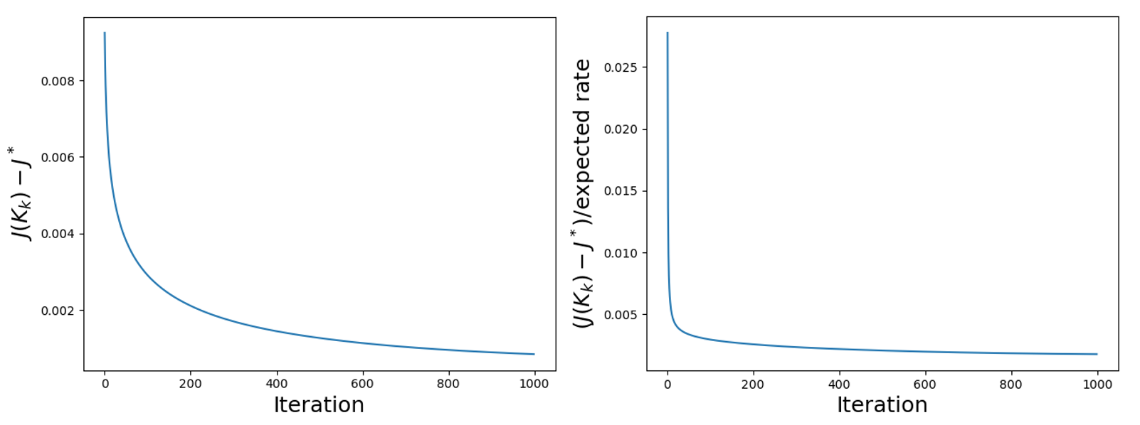
Figure 1: Convergence rate of $J(K_{k})-J^{\star}$ under Algorithm 2

7 Proof of Main results

For the simplicity of notation, we define

$$\begin{aligned} &\widebar{\Delta H_{k}}\triangleq H(\theta_{k},\omega_{k},X_{k})-H(\theta_{k},\omega^{\star}(\theta_{k}),X_{k})\\ &\Delta H_{k}\triangleq H(\theta_{k},\omega^{\star}(\theta_{k}),X_{k})-\mathbb{E}_{\hat{X}\sim\mu_{\theta_{k}}}[H(\theta_{k},\omega^{\star}(\theta_{k}),\hat{X})]\\ &\Delta G_{k}\triangleq G(\theta_{k},\omega_{k},X_{k})-\mathbb{E}_{\hat{X}\sim\mu_{\theta_{k}}}[G(\theta_{k},\omega_{k},\hat{X})]\\ &z_{k}\triangleq\omega_{k}-\omega^{\star}(\theta_{k}).\end{aligned}$$ (68)

The quantity $\widebar{\Delta H}_{k}$ reflects the error in $H$ from the inaccurate auxiliary variable, while $\Delta H_{k}$ and $\Delta G_{k}$ represent the errors the Markovian samples cause to $H$ and $G$.

An important step in our analysis is to characterize the convergence of the iterate $\omega_{k}$ to $\omega^{\star}(\theta_{k})$. We state this result in the following proposition.

Proposition 1

Under Assumptions 1-6, we have for all $k\geq{\cal K}$

$$\mathbb{E}[\|\omega_{k+1}-\omega^{\star}(\theta_{k+1})\|^{2}] \leq(1-\frac{\lambda_{G}\beta_{k}}{2})\mathbb{E}[\|\omega_{k}-\omega^{\star}(\theta_{k})\|^{2}]+C_{2}\tau_{k}^{2}\beta_{k-\tau_{k}}\beta_{k}\mathbb{E}\left[\|\theta_{k}\|^{2}\right]$$

$$\hskip 20.0pt+\frac{2L^{2}B^{2}\alpha_{k}^{2}}{\lambda_{G}\beta_{k}}+C_{2}\tau_{k}^{2}\beta_{k-\tau_{k}}\beta_{k},$$

where $C_{1}=18D^{2}+7LDB+9LD+LB+3D$ and $C_{2}=(4D^{2}+1)(4C_{1}+32D^{2})+\frac{2L^{2}B^{2}}{\lambda_{G}}+2L^{2}B^{2}$.

Proposition 1 shows the step-wise convergence of the auxiliary variable $\|z_{k}\|^{2}$ and its dependency on the decision variable iterates. In the following propositions, we provide intermediate results towards the proofs of the theorems that characterize the step-wise convergence of the decision variable. These propositions reveal the effect of the auxiliary variable on the convergence of the decision variables, and together with Proposition 1 implies that the convergence of the decision variable and the auxiliary variable forms a coupled dynamical system.

Proposition 2

Under the conditions of Proposition 1, we have for all $k\geq\tau_{k}$

$$\mathbb{E}\left[\|\theta_{k+1}-\theta^{\star}\|^{2}\right] \leq\left(1+C_{3}\tau_{k}^{2}\alpha_{k-\tau_{k}}\alpha_{k}\right)\mathbb{E}\left[\|\theta_{k}-\theta^{\star}\|^{2}\right]+(3C_{3}+B^{2})\tau_{k}^{2}\alpha_{k-\tau_{k}}\alpha_{k}$$

$$\hskip 20.0pt-2\alpha_{k}\mathbb{E}\left[\langle\theta_{k}-\theta^{\star},\nabla f(\theta_{k})\rangle\right]-2\alpha_{k}\mathbb{E}\left[\langle\theta_{k}-\theta^{\star},\widebar{\Delta H_{k}}\rangle\right],$$

where $C_{3}=4\left(BL^{2}+B^{2}L^{2}+B^{2}L+B+B^{2}+L^{2}\right)$.

Proposition 2 will be used in the convergence proof for strongly convex and convex functions. The dependency on the auxiliary variable is captured by the term $\mathbb{E}\left[\langle\theta_{k}-\theta^{\star},\widebar{\Delta H_{k}}\rangle\right]$. Later we will decompose and bound this term in different manners in the proofs of Theorem 1 and 2.

Proposition 3

Under the conditions of Proposition 1, we have for all $k\geq\tau_{k}$

$$\mathbb{E}[f(\theta_{k+1})] \leq\mathbb{E}[f(\theta_{k})]-\frac{\alpha_{k}}{2}\mathbb{E}[\|\nabla f(\theta_{k})\|^{2}]+\frac{L^{2}\alpha_{k}}{2}\mathbb{E}\left[\|z_{k}\|^{2}\right]+(C_{5}+\frac{LB^{2}}{2})\tau_{k}^{2}\alpha_{k}\alpha_{k-\tau_{k}},$$

where $C_{5}=4B^{3}L+4B^{2}L+2B^{2}L^{2}+2B^{2}$.

Proposition 3 will be used in the convergence proof for non-convex functions and functions with the PŁ condition. The effect of the auxiliary variable is obviously reflected by the term $\mathbb{E}\left[\|z_{k}\|^{2}\right]$.

We also introduce Lemma 3, which is helpful in bounding the sum of various step size sequences.

Lemma 3

a) Given a constant $u\in(0,1)$, we have for any $k\geq 0$

$$\frac{C_{u}(k+1)^{1-u}}{1-u}\leq\sum_{t=0}^{k}\frac{1}{(t+1)^{u}}\leq\frac{(k+1)^{1-u}}{1-u},$$

where $C_{u}=1-\frac{1}{2^{1-u}}$.

b) Given a constant $u>1$, we have for any $k\geq 0$

$$\sum_{t=0}^{k}\frac{1}{(t+1)^{u}}\leq\frac{u}{u-1},\quad\text{and}\quad\sum_{t=0}^{k}\frac{\log^{2}(t+1)}{(t+1)^{u}}\leq\frac{(u-1)^{3}+2}{(u-1)^{3}}.$$

c) For $u=1$, we have for any $k\geq 0$,

$$\sum_{t=0}^{k}\frac{1}{(t+1)^{u}}\leq\frac{\log(k+2)}{\log(2)}.$$

7.1 Proof of Theorem 1

From Proposition 2, we have for all $k\geq{\cal K}$

$$\mathbb{E}\left[\|\theta_{k+1}-\theta^{\star}\|^{2}\right] \leq\left(1+C_{3}\tau_{k}^{2}\alpha_{k-\tau_{k}}\alpha_{k}\right)\mathbb{E}\left[\|\theta_{k}-\theta^{\star}\|^{2}\right]+(3C_{3}+B^{2})\tau_{k}^{2}\alpha_{k-\tau_{k}}\alpha_{k}$$

$$\hskip 20.0pt-2\alpha_{k}\mathbb{E}\left[\langle\theta_{k}-\theta^{\star},\nabla f(\theta_{k})\rangle\right]-2\alpha_{k}\mathbb{E}\left[\langle\theta_{k}-\theta^{\star},\widebar{\Delta H_{k}}\rangle\right].$$ (69)

First, recall that $z_{k}=\omega_{k}-\omega^{\star}(\theta_{k})$. Using the relation $\langle v_{1},v_{2}\rangle\leq\frac{c}{2}\|v_{1}\|^{2}+\frac{1}{2c}\|v_{2}\|^{2}$ for any vector $v_{1},v_{2}$ and scalar $c>0$, we bound the last term of (69)

$$-\mathbb{E}\left[\langle\theta_{k}-\theta^{\star},\widebar{\Delta H_{k}}\rangle\right] \leq\frac{\lambda_{f}}{2}\mathbb{E}\left[\|\theta_{k}-\theta^{\star}\|^{2}\right]+\frac{1}{2\lambda_{f}}\mathbb{E}\left[\|H(\theta_{k},\omega_{k},X_{k})-H(\theta_{k},\omega^{\star}(\theta_{k}),X_{k})\|^{2}\right]$$

$$\leq\frac{\lambda_{f}}{2}\mathbb{E}\left[\|\theta_{k}-\theta^{\star}\|^{2}\right]+\frac{L^{2}}{2\lambda_{f}}\mathbb{E}\left[\|z_{k}\|^{2}\right],$$ (70)

where the last inequality follows from the Lipschitzness of the operator $H$. Next, we use the strong convexity of $f$ to handle the third term of (69)as

$$\langle\theta_{k}-\theta^{\star},\nabla f(\theta_{k})\rangle =\langle\theta_{k}-\theta^{\star},\nabla f(\theta_{k})-\nabla f(\theta^{\star})\rangle\geq\lambda_{f}\|\theta_{k}-\theta^{\star}\|^{2}.$$ (71)

Thus, using (70) and (71) into (69) we obtain

$$\mathbb{E}\left[\|\theta_{k+1}-\theta^{\star}\|^{2}\right]$$

$$\leq\left(1-\lambda_{f}\alpha_{k}+C_{3}\tau_{k}^{2}\alpha_{k-\tau_{k}}\alpha_{k}\right)\mathbb{E}\left[\|\theta_{k}-\theta^{\star}\|^{2}\right]$$

$$\hskip 20.0pt+(3C_{3}+B^{2})\tau_{k}^{2}\alpha_{k-\tau_{k}}\alpha_{k}+\frac{L^{2}\alpha_{k}}{\lambda_{f}}\mathbb{E}[\|z_{k}\|^{2}]$$

$$\leq(1-\frac{\lambda_{f}\alpha_{k}}{2})\mathbb{E}\left[\|\theta_{k}-\theta^{\star}\|^{2}\right]+\frac{L^{2}\alpha_{k}}{\lambda_{f}}\mathbb{E}\left[\|z_{k}\|^{2}\right]+(3C_{3}+B^{2})\tau_{k}^{2}\alpha_{k-\tau_{k}}\alpha_{k},$$ (72)

where the last inequality uses the step size condition $\tau_{k}^{2}\alpha_{k-\tau_{k}}\leq\frac{\lambda_{f}}{2C_{3}}$.

By Proposition 1, we have

$$\mathbb{E}[\|z_{k+1}\|^{2}] \leq(1-\frac{\lambda_{G}\beta_{k}}{2})\mathbb{E}[\|z_{k}\|^{2}]+C_{2}\tau_{k}^{2}\beta_{k-\tau_{k}}\beta_{k}\mathbb{E}\left[\|\theta_{k}\|^{2}\right]+\frac{2L^{2}B^{2}\alpha_{k}^{2}}{\lambda_{G}\beta_{k}}+C_{2}\tau_{k}^{2}\beta_{k-\tau_{k}}\beta_{k}$$

$$\leq(1-\frac{\lambda_{G}\beta_{k}}{2})\mathbb{E}[\|z_{k}\|^{2}]+2C_{2}\tau_{k}^{2}\beta_{k-\tau_{k}}\beta_{k}\mathbb{E}\left[\|\theta_{k}-\theta^{\star}\|^{2}\right]$$

$$\hskip 20.0pt+\frac{2L^{2}B^{2}\alpha_{k}^{2}}{\lambda_{G}\beta_{k}}+C_{2}\tau_{k}^{2}\beta_{k-\tau_{k}}\beta_{k}(2\|\theta^{\star}\|^{2}+1),$$ (73)

Applying Lemma 1 case a) with $\tau={\cal K}$ to (72) and (73) where

$$x_{k}=\mathbb{E}\left[\|\theta_{k}-\theta^{\star}\|^{2}\right],\quad y_{k}=\mathbb{E}\left[\|z_{k}\|^{2}\right],$$

$$a_{k}=\frac{\lambda_{f}\alpha_{k}}{2},\quad b_{k}=\frac{L^{2}\alpha_{k}}{\lambda_{f}},\quad c_{k}=(3C_{3}+B^{2})\tau_{k}^{2}\alpha_{k-\tau_{k}}\alpha_{k},$$

$$d_{k}=\frac{\lambda_{G}\beta_{k}}{2},\quad e_{k}=2C_{2}\tau_{k}^{2}\beta_{k-\tau_{k}}\beta_{k},\quad f_{k}=\frac{2L^{2}B^{2}\alpha_{k}^{2}}{\lambda_{G}\beta_{k}}+C_{2}\tau_{k}^{2}\beta_{k-\tau_{k}}\beta_{k}(2\|\theta^{\star}\|^{2}+1).$$

In this case, one can choose $A=\frac{4L^{2}}{\lambda_{f}^{2}}$ if the step size sequences satisfy

$$\tau_{k}^{2}\beta_{k-\tau_{k}}\leq\frac{\lambda_{f}^{2}\lambda_{G}}{32L^{2}C_{2}}\quad\text{and}\quad\frac{\alpha_{k}}{\beta_{k}}\leq\frac{\lambda_{G}}{2\lambda_{f}}.$$

Then we have for all $k\geq{\cal K}$

$$\mathbb{E}\left[\|\theta_{k}-\theta^{\star}\|^{2}\right]$$

$$\leq\left(\mathbb{E}\left[\|\theta_{{\cal K}}-\theta^{\star}\|^{2}\right]+\frac{4L^{2}\alpha_{{\cal K}}}{\lambda_{G}\lambda_{f}\beta_{{\cal K}}}\mathbb{E}[\|z_{{\cal K}}\|^{2}]\right)\prod_{t={\cal K}}^{k-1}(1-\frac{\lambda_{f}\alpha_{t}}{4})$$

$$+\sum_{\ell={\cal K}}^{k-1}\left((3C_{3}+B^{2})\tau_{k}^{2}\alpha_{\ell-\tau_{k}}\alpha_{\ell}+\frac{8L^{4}B^{2}\alpha_{\ell}^{3}}{\lambda_{G}^{2}\lambda_{f}\beta_{\ell}^{2}}+\frac{4L^{2}C_{2}\tau_{k}^{2}\beta_{\ell-\tau_{k}}\alpha_{\ell}}{\lambda_{G}\lambda_{f}}(2\|\theta^{\star}\|^{2}+1)\right)\prod_{t=\ell+1}^{k-1}(1-\frac{\lambda_{f}\alpha_{t}}{4})$$

$$\leq\left(\mathbb{E}\left[\|\theta_{{\cal K}}-\theta^{\star}\|^{2}\right]+\frac{4L^{2}\alpha_{{\cal K}}}{\lambda_{G}\lambda_{f}\beta_{{\cal K}}}\mathbb{E}[\|z_{{\cal K}}\|^{2}]\right)\prod_{t={\cal K}}^{k-1}(1-\frac{\lambda_{f}\alpha_{t}}{4})$$ (74)

$$+\sum_{\ell={\cal K}}^{k-1}\left((3C_{3}+B^{2}+\frac{4L^{2}C_{2}}{\lambda_{G}\lambda_{f}}(2\|\theta^{\star}\|^{2}+1))\tau_{k}^{2}\alpha_{\ell-\tau_{k}}\beta_{\ell}+\frac{8L^{4}B^{2}\alpha_{\ell}^{3}}{\lambda_{G}^{2}\lambda_{f}\beta_{\ell}^{2}}\right)\prod_{t=\ell+1}^{k-1}(1-\frac{\lambda_{f}\alpha_{t}}{4}).$$

Since $1+x\leq\text{exp}(x)$ for all $x\geq 0$, we have

$$\prod_{t={\cal K}}^{k-1}(1-\frac{\lambda_{f}\alpha_{t}}{4}) \leq\prod_{t={\cal K}}^{k-1}\text{exp}(-\frac{\lambda_{f}\alpha_{t}}{4})=\text{exp}(-\sum_{t={\cal K}}^{k-1}\frac{\lambda_{f}\alpha_{t}}{4})\leq\text{exp}(-\frac{\lambda_{f}\alpha_{0}}{4}\sum_{t={\cal K}}^{k-1}\frac{1}{t+1})$$

$$\leq\text{exp}(-\frac{\lambda_{f}\alpha_{0}}{4}\log(\frac{k+1}{{\cal K}+1}))\leq(\frac{{\cal K}+1}{k+1})^{\frac{\lambda_{f}\alpha_{0}}{4}}\leq\frac{{\cal K}+1}{k+1},$$ (75)

where the last inequality results from $\alpha_{0}\geq\frac{4}{\lambda_{f}}$, and the third inequality comes from

$$\sum_{t=k_{1}}^{k_{2}}\frac{1}{t+1}\geq\int_{k_{1}}^{k_{2}+1}\frac{1}{t+1}dt=\log(\frac{k_{2}+2}{k_{1}+1}).$$

Similarly,

$$\prod_{t=\ell+1}^{k-1}(1-\frac{\lambda_{f}\alpha_{t}}{4})\leq\frac{\ell+2}{k+1}\leq\frac{2(\ell+1)}{k+1}.$$ (76)

Using (75) and (76) in (74),

$$\mathbb{E}\left[\|\theta_{k}-\theta^{\star}\|^{2}\right]$$

$$\leq\left(\mathbb{E}\left[\|\theta_{{\cal K}}-\theta^{\star}\|^{2}\right]+\frac{4L^{2}\alpha_{{\cal K}}}{\lambda_{G}\lambda_{f}\beta_{{\cal K}}}\mathbb{E}[\|z_{{\cal K}}\|^{2}]\right)\frac{{\cal K}+1}{k+1}$$

$$+\sum_{\ell={\cal K}}^{k-1}\left((6C_{3}+2B^{2}+\frac{8L^{2}C_{2}}{\lambda_{G}\lambda_{f}}(2\|\theta^{\star}\|^{2}+1))\tau_{k}^{2}\alpha_{\ell-\tau_{k}}\beta_{\ell}+\frac{16L^{4}B^{2}\alpha_{\ell}^{3}}{\lambda_{G}^{2}\lambda_{f}\beta_{\ell}^{2}}\right)\frac{\ell+1}{k+1}.$$ (77)

Using the step sizes $\alpha_{k},\beta_{k}$ to the second term on the right-hand side of (77) we have

$$\sum_{\ell={\cal K}}^{k-1}\left((6C_{3}+2B^{2}+\frac{8L^{2}C_{2}}{\lambda_{G}\lambda_{f}}(2\|\theta^{\star}\|^{2}+1))\tau_{k}^{2}\alpha_{\ell-\tau_{k}}\beta_{\ell}+\frac{16L^{4}B^{2}\alpha_{\ell}^{3}}{\lambda_{G}^{2}\lambda_{f}\beta_{\ell}^{2}}\right)\frac{\ell+1}{k+1}$$

$$\leq\frac{\tau_{k}^{2}}{k+1}\left((6C_{3}+2B^{2}+\frac{8L^{2}C_{2}}{\lambda_{G}\lambda_{f}}(2\|\theta^{\star}\|^{2}+1))\frac{\alpha_{0}\beta_{0}}{c_{\tau}}+\frac{16L^{4}B^{2}\alpha_{0}^{3}}{\lambda_{G}^{2}\lambda_{f}\beta_{0}^{2}}\right)\sum_{\ell={\cal K}}^{k-1}\frac{\ell+1}{(\ell+1)^{5/3}}$$

$$\leq\frac{\tau_{k}^{2}}{k+1}\left((6C_{3}+2B^{2}+\frac{8L^{2}C_{2}}{\lambda_{G}\lambda_{f}}(2\|\theta^{\star}\|^{2}+1))\frac{\alpha_{0}\beta_{0}}{c_{\tau}}+\frac{16L^{4}B^{2}\alpha_{0}^{3}}{\lambda_{G}^{2}\lambda_{f}\beta_{0}^{2}}\right)\sum_{\ell=0}^{k}\frac{1}{(\ell+1)^{2/3}}$$

$$\leq\frac{\tau_{k}^{2}}{3(k+1)^{2/3}}\left((6C_{3}+2B^{2}+\frac{8L^{2}C_{2}}{\lambda_{G}\lambda_{f}}(2\|\theta^{\star}\|^{2}+1))\frac{\alpha_{0}\beta_{0}}{c_{\tau}}+\frac{16L^{4}B^{2}\alpha_{0}^{3}}{\lambda_{G}^{2}\lambda_{f}\beta_{0}^{2}}\right),$$ (78)

where the last inequality is due to Lemma 3 case a) with $u=2/3$. Using (78) in (77), we obtain our desired result, i.e.,

$$\mathbb{E}\left[\|\theta_{k}-\theta^{\star}\|^{2}\right] \leq\frac{{\cal K}+1}{k+1}\left(\mathbb{E}\left[\|\theta_{{\cal K}}-\theta^{\star}\|^{2}\right]+\frac{4L^{2}\alpha_{0}}{\lambda_{G}\lambda_{f}\beta_{0}}\mathbb{E}[\|\omega_{{\cal K}}-\omega^{\star}(\theta_{{\cal K}})\|^{2}]\right)$$

$$+\frac{\tau_{k}^{2}}{3(k+1)^{2/3}}\left((6C_{3}+2B^{2}+\frac{8L^{2}C_{2}}{\lambda_{G}\lambda_{f}}(2\|\theta^{\star}\|^{2}+1))\frac{\alpha_{0}\beta_{0}}{c_{\tau}}+\frac{16L^{4}B^{2}\alpha_{0}^{3}}{\lambda_{G}^{2}\lambda_{f}\beta_{0}^{2}}\right).$$

7.2 Proof of Theorem 2

Proposition 2 states that for all $k\geq\tau_{k}$

$$\mathbb{E}\left[\|\theta_{k+1}-\theta^{\star}\|^{2}\right] \leq\left(1+C_{3}\tau_{k}^{2}\alpha_{k-\tau_{k}}\alpha_{k}\right)\mathbb{E}\left[\|\theta_{k}-\theta^{\star}\|^{2}\right]+(3C_{3}+B^{2})\tau_{k}^{2}\alpha_{k-\tau_{k}}\alpha_{k}$$

$$\hskip 20.0pt-2\alpha_{k}\mathbb{E}\left[\langle\theta_{k}-\theta^{\star},\nabla f(\theta_{k})\rangle\right]-2\alpha_{k}\mathbb{E}\left[\langle\theta_{k}-\theta^{\star},\widebar{\Delta H_{k}}\rangle\right].$$ (79)

From the convexity of $f$, we have

$$\left\langle\theta^{\star}-\theta_{k},\nabla f\left(\theta_{k}\right)\right\rangle\leq f^{\star}-f(\theta_{k}).$$

Using $\widebar{\Delta H_{k}}$ defined in (68) and the relation $2xy\leq\eta x^{2}+1/\eta y^{2}$, for all $\eta>0,x,y$,

$$-2\alpha_{k}\mathbb{E}\left[\langle\theta_{k}-\theta^{\star},\widebar{\Delta H_{k}}\rangle\right]=-2\alpha_{k}\mathbb{E}\left[\langle\theta_{k}-\theta^{\star},H(\theta_{k},\omega_{k},X_{k})-H(\theta_{k},\omega^{\star}(\theta_{k}),X_{k})\rangle\right]$$

$$\leq\frac{2L^{2}\alpha_{k}^{2}}{\lambda_{G}\beta_{k}}\mathbb{E}[\|\theta_{k}-\theta^{\star}\|^{2}]+\frac{\lambda_{G}\beta_{k}}{2L^{2}}\mathbb{E}[\|H(\theta_{k},\omega_{k},X_{k})-H(\theta_{k},\omega^{\star}(\theta_{k}),X_{k})\|^{2}]$$

$$\leq\frac{2L^{2}\alpha_{k}^{2}}{\lambda_{G}\beta_{k}}\mathbb{E}[\|\theta_{k}-\theta^{\star}\|^{2}]+\frac{\lambda_{G}\beta_{k}}{2}\|z_{k}\|^{2}.$$

Using the preceding two relations into (79) implies

$$\mathbb{E}\left[\|\theta_{k+1}-\theta^{\star}\|^{2}\right] \leq\left(1+C_{3}\tau_{k}^{2}\alpha_{k-\tau_{k}}\alpha_{k}\right)\mathbb{E}\left[\|\theta_{k}-\theta^{\star}\|^{2}\right]+(3C_{3}+B^{2})\tau_{k}^{2}\alpha_{k-\tau_{k}}\alpha_{k}$$

$$\quad+2\alpha_{k}\mathbb{E}\left[f^{\star}-f(\theta_{k})\right]+\frac{2L^{2}\alpha_{k}^{2}}{\lambda_{G}\beta_{k}}\mathbb{E}[\|\theta_{k}-\theta^{\star}\|^{2}]+\frac{\lambda_{G}\beta_{k}}{2}\|z_{k}\|^{2}.$$ (80)

By Proposition 1 we have

$$\mathbb{E}[\|z_{k+1}\|^{2}]$$

$$\leq(1-\frac{\lambda_{G}\beta_{k}}{2})\mathbb{E}[\|z_{k}\|^{2}]+C_{2}\tau_{k}^{2}\beta_{k-\tau_{k}}\beta_{k}\mathbb{E}\left[\|\theta_{k}\|^{2}\right]+\frac{2L^{2}B^{2}\alpha_{k}^{2}}{\lambda_{G}\beta_{k}}+C_{2}\tau_{k}^{2}\beta_{k-\tau_{k}}\beta_{k}$$

$$\leq(1-\frac{\lambda_{G}\beta_{k}}{2})\mathbb{E}[\|z_{k}\|^{2}]+2C_{2}\tau_{k}^{2}\beta_{k-\tau_{k}}\beta_{k}\mathbb{E}\left[\|\theta_{k}-\theta^{\star}\|^{2}\right]$$

$$\quad+2C_{2}\|\theta^{\star}\|^{2}\tau_{k}^{2}\beta_{k-\tau_{k}}\beta_{k}+\frac{2L^{2}B^{2}\alpha_{k}^{2}}{\lambda_{G}\beta_{k}}+C_{2}\tau_{k}^{2}\beta_{k-\tau_{k}}\beta_{k}.$$ (81)

We define

$$V_{k}=\mathbb{E}\left[\|\theta_{k}-\theta^{\star}\|^{2}\right]+\mathbb{E}[\|z_{k}\|^{2}].$$

Combining (80) and (81), we obtain

$$V_{k+1} \leq V_{k}+\big{(}\frac{2L^{2}\alpha_{k}^{2}}{\lambda_{G}\beta_{k}}+2C_{2}\tau_{k}^{2}\beta_{k-\tau_{k}}\beta_{k}+C_{3}\tau_{k}^{2}\alpha_{k-\tau_{k}}\alpha_{k}\big{)}\mathbb{E}\left[\|\theta_{k}-\theta^{\star}\|^{2}\right]+2\alpha_{k}\mathbb{E}\left[f^{\star}-f(\theta_{k})\right]$$

$$\quad+2C_{2}\|\theta^{\star}\|^{2}\tau_{k}^{2}\beta_{k-\tau_{k}}\beta_{k}+\frac{2L^{2}B^{2}\alpha_{k}^{2}}{\lambda_{G}\beta_{k}}+C_{2}\tau_{k}^{2}\beta_{k-\tau_{k}}\beta_{k}+(3C_{3}+B^{2})\tau_{k}^{2}\alpha_{k-\tau_{k}}\alpha_{k}$$

$$\leq V_{k}+\big{(}\frac{2L^{2}\alpha_{k}^{2}}{\lambda_{G}\beta_{k}}+(2C_{2}+C_{3})\tau_{k}^{2}\beta_{k-\tau_{k}}\beta_{k}\big{)}V_{k}+2\alpha_{k}\mathbb{E}\left[f^{\star}-f(\theta_{k})\right]$$

$$\quad+C_{4}\tau_{k}^{2}\beta_{k-\tau_{k}}\beta_{k}+\frac{2L^{2}B^{2}\alpha_{k}^{2}}{\lambda_{G}\beta_{k}},$$

where we use the fact that $\alpha_{k}\leq\beta_{k}$ and $C_{4}$ is defined as

$$C_{4} =2C_{2}\|\theta^{\star}\|^{2}+C_{2}+3C_{3}+B^{2}.$$

Recall that $\alpha_{k}=\alpha_{0}$ and $\beta_{k}=\beta_{0}$, implying $\tau_{k}=\tau$. Let $\sigma$ be defined as

$$\sigma=1+\frac{2L^{2}\alpha_{0}^{2}}{\lambda_{G}\beta_{0}}+(2C_{2}+C_{3})\tau\beta_{0}^{2},$$

and $w_{k}=1/\sigma^{k}$. Multiplying both sides of the equation above by $w_{k+1}$ and rearranging we obtain

$$2w_{k+1}\alpha_{0}\mathbb{E}\left[f(\theta_{k})-f^{\star}\right]\leq w_{k}V_{k}-w_{k+1}V_{k+1}+\big{(}C_{4}\tau^{2}\beta_{0}^{2}+\frac{2L^{2}B^{2}\alpha_{0}^{2}}{\lambda_{G}\beta_{0}}\big{)}w_{k+1},$$

which when summing up both sides over $k$ from ${\cal K}$ to $T$ for some fixed $T>{\cal K}$ gives

$$2\alpha_{0}\sum_{k={\cal K}}^{T}w_{k+1}\mathbb{E}\left[f(\theta_{k})-f^{\star}\right]\leq w_{{\cal K}}V_{{\cal K}}-w_{T+1}V_{T+1}+\big{(}C_{4}\tau^{2}\beta_{0}^{2}+\frac{2L^{2}B^{2}\alpha_{0}^{2}}{\lambda_{G}\beta_{0}}\big{)}\sum_{k={\cal K}}^{T}w_{k+1}$$

Let ${\bar{\theta}}_{T}$ be defined as

$${\bar{\theta}}_{T}=\frac{\sum_{k={\cal K}}^{T}w_{k+1}\theta_{k}}{\sum_{k={\cal K}}^{T}w_{k+1}}.$$

Diving both sides of the equation above by $2\alpha_{0}\sum_{k={\cal K}}^{T}w_{k+1}$ and using the Jensen’s inequality yields

$$f({\bar{\theta}}_{T})-f^{\star}\leq\frac{w_{{\cal K}}V_{{\cal K}}}{2\alpha\sum_{k={\cal K}}^{T}w_{k+1}}+\frac{C_{4}\tau^{2}\beta_{0}^{2}}{2\alpha_{0}}+\frac{L^{2}B^{2}\alpha_{0}}{\lambda_{G}\beta_{0}}.$$

We choose $\alpha_{0}$ and $\beta_{0}$ as

$$\alpha_{0}=\sqrt{\frac{\lambda_{G}}{2L^{2}\sqrt{2C_{2}+C_{3}}}}\frac{1}{2C\log^{3/4}(T)T^{3/4}}\quad\text{ and }\quad\beta_{0}=\frac{1}{2C\sqrt{2C_{2}+C_{3}}\sqrt{\log(T)}\sqrt{T}},$$

which gives

$$2\alpha_{0}\sum_{k={\cal K}}^{T}w_{k+1}\geq 2\alpha_{0}(T-{\cal K})\min_{{\cal K}\leq k\leq T}w_{k+1}\geq 2\alpha_{0}(T-{\cal K})w_{T+1}=\frac{2\alpha_{0}(T-{\cal K})}{\sigma^{T+1}}.$$

Using $1+x\leq\exp(x)$ we consider

$$\sigma^{T} \leq\big{(}1+\frac{2L^{2}\alpha_{0}^{2}}{\lambda_{G}\beta_{0}}+(2C_{2}+C_{3})\tau\beta_{0}^{2}\big{)}^{T}\leq\exp\big{(}\frac{2L^{2}\alpha_{0}^{2}T}{\lambda_{G}\beta_{0}}+(2C_{2}+C_{3})\tau\beta_{0}^{2}T\big{)}$$

$$\leq\exp\big{(}\frac{1+\tau}{2C\log(T)}\big{)}\leq\exp\big{(}\frac{\tau}{C\log(T)}\big{)}\leq\exp\left(\frac{\log(1/\alpha_{0})}{\log(T)}\right)$$

$$=\exp\big{(}\log(\frac{2C\sqrt{2L^{2}\sqrt{2C_{2}+C_{3}}}}{\lambda_{G}})/\log(T)+\log(\log^{3/4}(T)T^{3/4})/\log{T}\big{)}$$

$$\leq\frac{2C\sqrt{2L^{2}\sqrt{2C_{2}+C_{3}}}}{\lambda_{G}}+3,$$

where the last inequality uses $T\geq e$ and $\exp(\log(\log^{3/4}(T)T^{3/4})/\log(T))\leq\exp(1.05)<3$ for all $T>0$. Thus we obtain

$$f({\bar{\theta}}_{T})-f^{\star} \leq\frac{(\frac{2C\sqrt{2L^{2}\sqrt{2C_{2}+C_{3}}}}{\lambda_{G}}+3)w_{{\cal K}}V_{{\cal K}}}{2\alpha_{0}(T-{\cal K})}+\frac{C_{4}L\tau^{2}\log^{1/2}(T)}{2C^{2}(2D+C_{3})^{3/4}\sqrt{\lambda_{G}}T^{1/4}}$$

$$\hskip 20.0pt+\frac{2L^{3}B^{2}(2D+3C_{3}^{1/4})}{\sqrt{\lambda_{G}}\log^{1/2}(T)T^{1/4}}.$$

7.3 Proof of Theorem 3

Proposition 3 states that for all $k\geq{\cal K}$

$$\mathbb{E}[f(\theta_{k+1})] \leq\mathbb{E}\left[f(\theta_{k})-\frac{\alpha_{k}}{2}\|\nabla f(\theta_{k})\|^{2}+\frac{L^{2}\alpha_{k}}{2}\|z_{k}\|^{2}\right]+(C_{5}+\frac{LB^{2}}{2})\tau_{k}^{2}\alpha_{k}\alpha_{k-\tau_{k}}.$$

By the PŁ condition, we have for all $\theta\in\mathbb{R}^{d}$

$$\frac{1}{2}\|\nabla f(\theta)\|^{2}\geq\lambda_{f}(f(\theta)-f^{\star}),$$

which implies that

$$\mathbb{E}[f(\theta_{k+1})] \leq\mathbb{E}\left[f(\theta_{k})-\frac{\alpha_{k}}{2}\|\nabla f(\theta_{k})\|^{2}+\frac{L^{2}\alpha_{k}}{2}\|z_{k}\|^{2}\right]+(C_{5}+\frac{LB^{2}}{2})\tau_{k}^{2}\alpha_{k}\alpha_{k-\tau_{k}}$$

$$\leq\mathbb{E}[f(\theta_{k})]-\lambda_{f}\alpha_{k}\mathbb{E}\left[f(\theta_{k})-f^{\star}\right]+\frac{L^{2}\alpha_{k}}{2}\mathbb{E}\left[\|z_{k}\|^{2}\right]+(C_{5}+\frac{LB^{2}}{2})\tau_{k}^{2}\alpha_{k}\alpha_{k-\tau_{k}}.$$

Subtracting $f^{\star}$ from both sides of the inequality and rearranging the terms, we get

$$\mathbb{E}[f(\theta_{k+1})-f^{\star}] \leq(1-\lambda_{f}\alpha_{k})\mathbb{E}[f(\theta_{k})-f^{\star}]+\frac{L^{2}\alpha_{k}}{2}\mathbb{E}\left[\|z_{k}\|^{2}\right]+(C_{5}+\frac{LB^{2}}{2})\tau_{k}^{2}\alpha_{k}\alpha_{k-\tau_{k}}.$$ (82)

On the other hand, from the analysis of the auxiliary variable in Proposition 1,

$$\mathbb{E}[\|z_{k+1}\|^{2}] \leq(1-\frac{\lambda_{G}\beta_{k}}{2})\mathbb{E}[\|z_{k}\|^{2}]+C_{2}\tau_{k}^{2}\beta_{k-\tau_{k}}\beta_{k}\mathbb{E}\left[\|\theta_{k}\|^{2}\right]+\frac{2L^{2}B^{2}\alpha_{k}^{2}}{\lambda_{G}\beta_{k}}+C_{2}\tau_{k}^{2}\beta_{k-\tau_{k}}\beta_{k}.$$ (83)

Choosing $a=1$, we can bound

$$\|\theta_{k}\|\leq\|\theta_{0}\|+\sum_{t=0}^{k-1}\|\theta_{t+1}-\theta_{t}\|\leq\|\theta_{0}\|+\sum_{t=0}^{k-1}\frac{B\alpha}{t+1}\leq\|\theta_{0}\|+\frac{B\alpha\log(k+1)}{\log(2)},$$

where the last inequality follows from Lemma 3 case c). This implies for any $k\geq 0$

$$\|\theta_{k}\|^{2}\leq 2\|\theta_{0}\|^{2}+\frac{2B^{2}\alpha^{2}\log^{2}(k+1)}{\log^{2}(2)}\leq 24(\|\theta_{0}\|^{2}+B^{2}\alpha^{2})\log^{2}(k+1).$$

Using this bound in (83), we have

$$\mathbb{E}[\|z_{k+1}\|^{2}] \leq(1-\frac{\lambda_{G}\beta_{k}}{2})\mathbb{E}[\|z_{k}\|^{2}]+C_{2}\tau_{k}^{2}\beta_{k-\tau_{k}}\beta_{k}\mathbb{E}\left[\|\theta_{k}\|^{2}\right]+\frac{2L^{2}B^{2}\alpha_{k}^{2}}{\lambda_{G}\beta_{k}}+C_{2}\tau_{k}^{2}\beta_{k-\tau_{k}}\beta_{k}$$

$$\leq(1-\frac{\lambda_{G}\beta_{k}}{2})\mathbb{E}[\|z_{k}\|^{2}]+24C_{2}(\|\theta_{0}\|^{2}+B^{2}\alpha^{2})\tau_{k}^{2}\beta_{k-\tau_{k}}\beta_{k}\log^{2}(k+1)$$

$$\hskip 20.0pt+\frac{2L^{2}B^{2}\alpha_{k}^{2}}{\lambda_{G}\beta_{k}}+C_{2}\tau_{k}^{2}\beta_{k-\tau_{k}}\beta_{k}$$

$$\leq(1-\frac{\lambda_{G}\beta_{k}}{2})\mathbb{E}[\|z_{k}\|^{2}]+24C_{2}(\|\theta_{0}\|^{2}+B^{2}\alpha^{2}+1)\tau_{k}^{2}\beta_{k-\tau_{k}}\beta_{k}\log^{2}(k+1)$$

$$\hskip 20.0pt+\frac{2L^{2}B^{2}\alpha_{k}^{2}}{\lambda_{G}\beta_{k}},$$ (84)

where in the last inequality simply re-combines the terms.

Viewing (82) and (84), we can apply Lemma 1 case a) with $\tau={\cal K}$ and

$$x_{k}=\mathbb{E}[f(\theta_{k})-f^{\star}],\quad y_{k}=\mathbb{E}\left[\|z_{k}\|^{2}\right],$$

$$a_{k}=\lambda_{f}\alpha_{k},\quad b_{k}=\frac{L^{2}\alpha_{k}}{2},\quad c_{k}=(C_{5}+\frac{LB^{2}}{2})\tau_{k}^{2}\alpha_{k}\alpha_{k-\tau_{k}},\quad d_{k}=\frac{\lambda_{G}\beta_{k}}{2},$$

$$e_{k}=0,\quad f_{k}=24C_{2}(\|\theta_{0}\|^{2}+B^{2}\alpha^{2}+1)\tau_{k}^{2}\beta_{k-\tau_{k}}\beta_{k}\log^{2}(k+1)+\frac{2L^{2}B^{2}\alpha_{k}^{2}}{\lambda_{G}\beta_{k}}.$$

In this case, one can verify that we can choose $A=\frac{L^{2}}{\lambda_{f}}$ if the step size sequences satisfy

$$\frac{\alpha_{k}}{\beta_{k}}\leq\frac{\lambda_{G}}{4\lambda_{f}}.$$

As a result of Lemma 1 case a), we have for all $k\geq{\cal K}$

$$\mathbb{E}\left[f(\theta_{k})-f^{\star}\right] \leq\left(\mathbb{E}\left[f(\theta_{{\cal K}})-f^{\star}\right]+\frac{2L^{2}\alpha_{{\cal K}}}{\lambda_{G}\beta_{{\cal K}}}\mathbb{E}[\|z_{{\cal K}}\|^{2}]\right)\prod_{t={\cal K}}^{k-1}(1-\frac{\lambda_{f}\alpha_{t}}{2})$$

$$+\sum_{\ell={\cal K}}^{k-1}\left((C_{5}+\frac{LB^{2}}{2})\tau_{k}^{2}\alpha_{\ell}\alpha_{\ell-\tau_{k}}+\frac{48C_{2}L^{2}}{\lambda_{G}}(\|\theta_{0}\|^{2}+B^{2}\alpha^{2}+1)\tau_{k}^{2}\beta_{k-\tau_{k}}\alpha_{k}\log^{2}(k+1)+\frac{4L^{4}B^{2}\alpha_{k}^{3}}{\lambda_{G}^{2}\beta_{k}^{2}}\right)$$

$$\hskip 150.0pt\times\prod_{t=\ell+1}^{k-1}(1-\frac{\lambda_{f}\alpha_{t}}{2}).$$

Plugging in the step sizes to the second term, we have

$$\mathbb{E}\left[f(\theta_{k})-f^{\star}\right] \leq\left(\mathbb{E}\left[f(\theta_{{\cal K}})-f^{\star}\right]+\frac{2L^{2}\alpha_{\tau_{k}}}{\lambda_{G}\beta_{\tau_{k}}}\mathbb{E}[\|z_{{\cal K}}\|^{2}]\right)\prod_{t={\cal K}}^{k-1}(1-\frac{\lambda_{f}\alpha_{t}}{2})$$

$$\hskip 10.0pt+\tau_{k}^{2}\sum_{\ell={\cal K}}^{k-1}\Big{(}(C_{5}+\frac{LB^{2}}{2})\frac{\alpha_{0}^{2}}{c_{\tau}(\ell+1)^{2}}+\frac{4L^{4}B^{2}\alpha_{0}^{3}}{\lambda_{G}^{2}\beta_{0}^{2}(\ell+1)^{5/3}}$$

$$\hskip 20.0pt+\frac{48C_{2}L^{2}}{\lambda_{G}}(\|\theta_{0}\|^{2}+B^{2}\alpha_{0}^{2}+1)\frac{\alpha_{0}\beta_{0}}{c_{\tau}(\ell+1)^{5/3}}\log^{2}(k+1)\Big{)}\prod_{t=\ell+1}^{k-1}(1-\frac{\lambda_{f}\alpha_{t}}{2})$$

$$\leq\left(\mathbb{E}\left[f(\theta_{{\cal K}})-f^{\star}\right]+\frac{2L^{2}\alpha_{{\cal K}}}{\lambda_{G}\beta_{{\cal K}}}\mathbb{E}[\|z_{{\cal K}}\|^{2}]\right)\prod_{t={\cal K}}^{k-1}(1-\frac{\lambda_{f}\alpha_{t}}{2})$$

$$\hskip 10.0pt+\tau_{k}^{2}\log^{2}(k+1)\sum_{\ell={\cal K}}^{k-1}\frac{C_{6}}{(\ell+1)^{5/3}}\prod_{t=\ell+1}^{k-1}(1-\frac{\lambda_{f}\alpha_{t}}{2}),$$ (85)

where we use the fact that $\frac{1}{\log^{2}(k+1)}\leq 12$ for all $k>0$ and define $C_{6}=(12C_{5}+6LB^{2})\frac{\alpha_{0}^{2}}{c_{\tau}}+\frac{48C_{2}L^{2}}{\lambda_{G}}(\|\theta_{0}\|^{2}+B^{2}\alpha_{0}^{2}+1)\frac{\alpha_{0}\beta_{0}}{c_{\tau}}+\frac{48L^{4}B^{2}\alpha_{0}^{3}}{\lambda_{G}^{2}\beta_{0}^{2}}$.

Since $1+x\leq\text{exp}(x)$ for all $x\geq 0$, we have

$$\prod_{t={\cal K}}^{k-1}(1-\frac{\lambda_{f}\alpha_{t}}{2}) \leq\prod_{t={\cal K}}^{k-1}\text{exp}(-\frac{\lambda_{f}\alpha_{t}}{2})=\text{exp}(-\sum_{t={\cal K}}^{k-1}\frac{\lambda_{f}\alpha_{t}}{2})\leq\text{exp}(-\frac{\lambda_{f}\alpha_{0}}{2}\sum_{t={\cal K}}^{k-1}\frac{1}{t+1})$$

$$\leq\text{exp}(-\frac{\lambda_{f}\alpha_{0}}{2}\log(\frac{k+1}{{\cal K}+1}))\leq(\frac{{\cal K}+1}{k+1})^{\frac{\lambda_{f}\alpha_{0}}{2}}\leq\frac{{\cal K}+1}{k+1},$$ (86)

where the last inequality results from $\alpha_{0}\geq\frac{2}{\lambda_{f}}$, and the third inequality comes from

$$\sum_{t=k_{1}}^{k_{2}}\frac{1}{t+1}\geq\int_{k_{1}}^{k_{2}+1}\frac{1}{t+1}dt=\log(\frac{k_{2}+2}{k_{1}+1}).$$

Similarly,

$$\prod_{t=\ell+1}^{k-1}(1-\frac{\lambda_{f}\alpha_{t}}{2})\leq\frac{2\ell+1}{k+1}\leq\frac{2(\ell+1)}{k+1}.$$ (87)

Using (86) and (87) in (85),

$$\mathbb{E}\left[f(\theta_{k})-f^{\star}\right] \leq\left(\mathbb{E}\left[f(\theta_{{\cal K}})-f^{\star}\right]+\frac{2L^{2}\alpha_{{\cal K}}}{\lambda_{G}\beta_{{\cal K}}}\mathbb{E}[\|z_{{\cal K}}\|^{2}]\right)\frac{{\cal K}}{k+1}+\frac{\log^{2}(k+1)\tau_{k}^{2}}{k+1}\sum_{\ell={\cal K}}^{k-1}\frac{2C_{6}}{(\ell+1)^{2/3}}$$

$$\leq\frac{{\cal K}+1}{k+1}\left(\mathbb{E}\left[f(\theta_{{\cal K}})-f^{\star}\right]+\frac{2L^{2}\alpha_{0}}{\lambda_{G}\beta_{0}}\mathbb{E}[\|z_{{\cal K}}\|^{2}]\right)+\frac{2C_{6}\log^{2}(k+1)\tau_{k}^{2}}{3(k+1)^{2/3}},$$

where the last inequality is from Lemma 3 case a).

7.4 Proof of Theorem 4

We first establish the following result that is similar to Proposition 1 but is stronger by using the more strict Assumption 9.

Proposition 4

Let the step size sequence $\{\beta_{k}\}$ satisfy the condition for all $k\geq\tau_{k}$

$$\beta_{k-\tau_{k}}\tau_{k}^{2}\leq\min\left\{1,\frac{1}{6LB},\frac{\lambda_{G}}{22C_{1}+16D^{2}}\right\}.$$ (88)

Then, under Assumptions 1-9, we have for all $k\geq\tau_{k}$

$$\mathbb{E}[\|\omega_{k+1}-\omega^{\star}(\theta_{k+1})\|^{2}] \leq(1-\frac{\lambda_{G}\beta_{k}}{2})\mathbb{E}[\|\omega_{k}-\omega^{\star}(\theta_{k})\|^{2}]+\frac{2L^{2}B^{2}\alpha_{k}^{2}}{\lambda_{G}\beta_{k}}+C_{7}\tau_{k}^{2}\beta_{k-\tau_{k}}\beta_{k},$$

where $C_{7}=(2B^{2}+1)(4C_{1}+4D^{2})+\frac{2L^{2}B^{2}}{\lambda_{G}}+2L^{2}B^{2}$.

In Proposition 3 and 4, we have established the following two inequalities for all $k\geq{\cal K}$

$$\mathbb{E}[f(\theta_{k+1})]\leq\mathbb{E}\left[f(\theta_{k})\right]+\frac{L^{2}\alpha_{k}}{2}\mathbb{E}\left[\|z_{k}\|^{2}\right]-\frac{\alpha_{k}}{2}\mathbb{E}\left[\|\nabla f(\theta_{k})\|^{2}\right]$$

$$\hskip 150.0pt+(C_{5}+\frac{LB^{2}}{2})\tau_{k}^{2}\alpha_{k}\alpha_{k-\tau_{k}},$$ (89)

$$\mathbb{E}[\|z_{k+1}\|^{2}]\leq(1-\frac{\lambda_{G}\beta_{k}}{2})\mathbb{E}[\|z_{k}\|^{2}]+\frac{2L^{2}B^{2}\alpha_{k}^{2}}{\lambda_{G}\beta_{k}}+C_{7}\tau_{k}^{2}\beta_{k-\tau_{k}}\beta_{k}.$$ (90)

We now apply Lemma 1 case b) to the coupled system (89) and (90) with $\tau={\cal K}$ and

$$x_{k}=\mathbb{E}[f(\theta_{k})-f(\theta^{\star})],\quad y_{k}=\mathbb{E}[\|z_{k}\|^{2}],\quad u_{k}=\frac{\alpha_{k}}{2}\mathbb{E}\left[\|\nabla f(\theta_{k})\|^{2}\right]$$

$$a_{k}=0,\quad b_{k}=\frac{L^{2}\alpha_{k}}{2},\quad c_{k}=(C_{5}+\frac{LB^{2}}{2})\tau_{k}^{2}\alpha_{k}\alpha_{k-\tau_{k}},$$

$$d_{k}=\frac{\lambda_{G}\beta_{k}}{2},\quad e_{k}=0,\quad f_{k}=\frac{2L^{2}B^{2}\alpha_{k}^{2}}{\lambda_{G}\beta_{k}}+C_{7}\tau_{k}^{2}\beta_{k-\tau_{k}}\beta_{k},$$

which yields

$$\sum_{t={\cal K}}^{k}\frac{\alpha_{t}}{2}\mathbb{E}\left[\|\nabla f(\theta_{k})\|^{2}\right] \leq\mathbb{E}[f(\theta_{{\cal K}})-f(\theta^{\star})]+\frac{L^{2}\alpha_{{\cal K}}}{\lambda_{G}\beta_{{\cal K}}}\mathbb{E}[\|z_{\tau_{k}}\|^{2}]+\sum_{t={\cal K}}^{k}(C_{5}+\frac{LB^{2}}{2})\tau_{k}^{2}\alpha_{k}\alpha_{k-\tau_{k}}$$

$$\hskip 20.0pt+\sum_{t={\cal K}}^{k}\frac{L^{2}\alpha_{t}}{\lambda_{G}\beta_{t}}\left(\frac{2L^{2}B^{2}\alpha_{t}^{2}}{\lambda_{G}\beta_{t}}+C_{7}\tau_{k}^{2}\beta_{t-\tau_{k}}\beta_{t}\right)$$ (91)

Plugging in the step sizes with $a=3/5$ and $b=2/5$, the last two terms in (91) become

$$\sum_{t={\cal K}}^{k}(C_{5}+\frac{LB^{2}}{2})\tau_{k}^{2}\alpha_{k}\alpha_{k-\tau_{k}}+\sum_{t={\cal K}}^{k}\frac{L^{2}\alpha_{t}}{\lambda_{G}\beta_{t}}\left(\frac{2L^{2}B^{2}\alpha_{t}^{2}}{\lambda_{G}\beta_{k}}+C_{7}\tau_{k}^{2}\beta_{t-\tau_{k}}\beta_{t}\right)$$

$$\leq\frac{\alpha_{0}^{2}(2C_{5}+LB^{2})}{2c_{\tau}}\sum_{t={\cal K}}^{k}\frac{\tau_{k}^{2}}{(t+1)^{6/5}}+\frac{2L^{4}B^{2}\alpha_{0}^{3}}{\lambda_{G}\beta_{0}^{2}}\sum_{t={\cal K}}^{k}\frac{1}{t+1}+\frac{L^{2}\alpha_{0}\beta_{0}C_{7}}{c_{\tau}\lambda_{G}}\sum_{t={\cal K}}^{k}\frac{\tau_{k}^{2}}{t+1}$$

$$\leq C_{8}\sum_{t={\cal K}}^{k}\frac{\tau_{k}^{2}}{t+1},$$ (92)

where in the last inequality we use the fact that $\tau_{k}\geq 1$ and define the constant $C_{8}=\frac{\alpha_{0}^{2}(2C_{5}+LB^{2})}{2c_{\tau}}+\frac{2L^{4}B^{2}\alpha_{0}^{3}}{\lambda_{G}\beta_{0}^{2}}+\frac{L^{2}\alpha_{0}\beta_{0}C_{7}}{c_{\tau}\lambda_{G}}$. From Lemma 3 case c),

$$\sum_{t={\cal K}}^{k}\frac{\tau_{k}^{2}}{t+1}\leq\sum_{t=0}^{k-{\cal K}}\frac{\tau_{k}^{2}}{t+1}\leq\tau_{k}^{2}\frac{\log(k-{\cal K}+2)}{\log(2)}\leq\frac{2\tau_{k}^{2}\log(k+1)}{5\log(2)}.$$

Using this inequality in (92), we have

$$\sum_{t={\cal K}}^{k}(C_{5}+\frac{LB^{2}}{2})\tau_{k}^{2}\alpha_{k}\alpha_{k-\tau_{k}}+\sum_{t={\cal K}}^{k}\frac{L^{2}\alpha_{t}}{\lambda_{G}\beta_{t}}\left(\frac{2L^{2}B^{2}\alpha_{t}^{2}}{\lambda_{G}\beta_{k}}+C_{2}(B_{\theta}^{2}+1)\tau_{k}^{2}\beta_{t-\tau_{k}}\beta_{t}\right)$$

$$\leq C_{8}\sum_{t={\cal K}}^{k}\frac{\tau_{k}^{2}}{t+1}\leq\frac{2C_{8}\tau_{k}^{2}\log(k+1)}{5\log(2)}.$$ (93)

Combining (91) and (93) leads to

$$\sum_{t={\cal K}}^{k}\frac{\alpha_{t}}{2}\mathbb{E}\left[\|\nabla f(\theta_{k})\|^{2}\right] \leq\mathbb{E}[f(\theta_{{\cal K}})-f(\theta^{\star})]+\frac{L^{2}\alpha_{{\cal K}}}{\lambda_{G}\beta_{{\cal K}}}\mathbb{E}[\|z_{{\cal K}}\|^{2}]+\frac{2C_{8}\tau_{k}^{2}\log(k+1)}{5\log(2)}.$$ (94)

Since by Lemma 3 case a) we have

$$\sum_{t^{\prime}={\cal K}}^{k}\alpha_{t^{\prime}}=\alpha_{0}\sum_{t^{\prime}=0}^{k-{\cal K}}(\frac{1}{t^{\prime}+{\cal K}})^{a}\geq(1-\frac{1}{2^{2/5}})\frac{\alpha_{0}(k+1)^{1-a}}{1-a}\geq\frac{\alpha_{0}(k+1)^{2/5}}{2},$$

the inequality (94) further implies for all $k\geq{\cal K}$

$$\min_{t\leq k}\mathbb{E}[\|\nabla f(\theta_{t})\|^{2}] \leq\frac{1}{\sum_{t^{\prime}={\cal K}}^{k}\alpha_{t^{\prime}}}\sum_{t={\cal K}}^{k}\alpha_{t}\mathbb{E}[\|\nabla f(\theta_{t})\|^{2}]$$

$$\leq\frac{4}{\alpha_{0}(k+1)^{2/5}}\mathbb{E}[f(\theta_{{\cal K}})-f^{\star}]+\frac{4L^{2}}{\beta_{0}\lambda_{G}(k+1)^{2/5}}\mathbb{E}[\|z_{{\cal K}}\|^{2}]+\frac{8C_{8}\tau_{k}^{2}\log(k+1)}{5\log(2)c_{\tau}(k+1)^{2/5}}.$$

Appendix A Proof of Propositions and Theorems

A.1 Proof of Proposition 1

We introduce the following technical lemmas.

Lemma 4

Under Assumption 1, we have for all $\theta\in\mathbb{R}^{d},\omega\in\mathbb{R}^{r},X\in{\cal X}$

$$\|G(\theta,\omega,X)\|\leq D(\|\theta\|+\|\omega\|+1).$$

Lemma 5

We have for all $\theta\in\mathbb{R}^{d}$

$$\|\omega^{\star}(\theta)\|\leq D(\|\theta\|+1).$$

Lemma 6

For all $k\geq\tau_{k}$, we have

$$\|\omega_{k}-\omega_{k-\tau_{k}}\| \leq 3D\beta_{k-\tau_{k}}\tau_{k}\left(\|\omega_{k}\|+\|\theta_{k}\|+1\right).$$

Lemma 7

For any $k\geq\tau_{k}$, we have

$$\mathbb{E}[\langle z_{k},\Delta G_{k}\rangle]\leq C_{1}\tau_{k}^{2}\beta_{k-\tau_{k}}\mathbb{E}\left[\|z_{k-\tau_{k}}\|^{2}+\|\theta_{k}\|^{2}+\|\omega_{k}\|^{2}+1\right],$$

where $C_{1}=18D^{2}+7LDB+9LD+LB+3D$.

Recall that $z_{k}=\omega_{k}-\omega^{\star}(\theta_{k})$. Using (8) gives

$$\|z_{k+1}\|^{2} =\|\omega_{k}+\beta_{k}G(\theta_{k+1},\omega_{k},X_{k})-\omega^{\star}(\theta_{k+1})\|^{2}$$

$$=\|\left(\omega_{k}-\omega^{\star}(\theta_{k})\right)+\beta_{k}G(\theta_{k+1},\omega_{k},X_{k})+\left(\omega^{\star}(\theta_{k})-\omega^{\star}(\theta_{k+1})\right)\|^{2}$$

$$=\|z_{k}\|^{2}+2\beta_{k}\langle z_{k},G(\theta_{k+1},\omega_{k},X_{k})\rangle+2\langle z_{k},\omega^{\star}(\theta_{k})-\omega^{\star}(\theta_{k+1})\rangle$$

$$\qquad+\|\beta_{k}G(\theta_{k+1},\omega_{k},X_{k})+\omega^{\star}(\theta^{k})-\omega^{\star}(\theta^{k+1})\|^{2}$$

$$\leq\|z_{k}\|^{2}+2\beta_{k}\langle z_{k},G(\theta_{k+1},\omega_{k},X_{k})\rangle+2\langle z_{k},\omega^{\star}(\theta_{k})-\omega^{\star}(\theta_{k+1})\rangle$$

$$\qquad+2\beta_{k}^{2}\left\|G(\theta_{k+1},\omega_{k},X_{k})\right\|^{2}+2\|\omega^{\star}(\theta^{k})-\omega^{\star}(\theta^{k+1})\|^{2}.$$

Recall from (68) that

$$\Delta G_{k}\triangleq G(\theta_{k},\omega_{k},X_{k})-\mathbb{E}_{\hat{X}\sim\mu_{\theta_{k}}}[G(\theta_{k},\omega_{k},\hat{X})],$$

which when using into the equation above gives

$$\|z_{k+1}\|^{2}$$

$$\leq\|z_{k}\|^{2}+2\beta_{k}\langle z_{k},G(\theta_{k+1},\omega_{k},X_{k})-G(\theta_{k},\omega_{k},X_{k})\rangle+2\beta_{k}\langle z_{k},G(\theta_{k},\omega_{k},X_{k})\rangle$$

$$\qquad+2\langle z_{k},\omega^{\star}(\theta_{k})-\omega^{\star}(\theta_{k+1})\rangle+2\beta_{k}^{2}\left\|G(\theta_{k+1},\omega_{k},X_{k})\right\|^{2}+2\|\omega^{\star}(\theta^{k})-\omega^{\star}(\theta^{k+1})\|^{2}$$

$$=\|z_{k}\|^{2}+2\beta_{k}\langle z_{k},G(\theta_{k+1},\omega_{k},X_{k})-G(\theta_{k},\omega_{k},X_{k})\rangle+2\beta_{k}\langle z_{k},\mathbb{E}_{\hat{X}\sim\mu_{\theta_{k}}}[G(\theta_{k},\omega_{k},\hat{X})]\rangle$$

$$\qquad+2\beta_{k}\langle z_{k},\Delta G_{k}\rangle+2\langle z_{k},\omega^{\star}(\theta_{k})-\omega^{\star}(\theta_{k+1})\rangle$$

$$\qquad+2\beta_{k}^{2}\left\|G(\theta_{k+1},\omega_{k},X_{k})\right\|^{2}+2\|\omega^{\star}(\theta^{k})-\omega^{\star}(\theta^{k+1})\|^{2}$$

$$\leq\|z_{k}\|^{2}+2\beta_{k}\langle z_{k},G(\theta_{k+1},\omega_{k},X_{k})-G(\theta_{k},\omega_{k},X_{k})\rangle+2\beta_{k}\langle z_{k},\mathbb{E}_{\hat{X}\sim\mu_{\theta_{k}}}[G(\theta_{k},\omega_{k},\hat{X})]\rangle$$

$$\qquad+2\beta_{k}\langle z_{k},\Delta G_{k}\rangle+2\langle z_{k},\omega^{\star}(\theta_{k})-\omega^{\star}(\theta_{k+1})\rangle$$

$$\qquad+2\beta_{k}^{2}\left\|G(\theta_{k+1},\omega_{k},X_{k})\right\|^{2}+2L^{2}B^{2}\alpha_{k}^{2},$$ (95)

where the last inequality follows from Assumption 1 and (7), i.e.,

$$\|\omega^{\star}(\theta_{k})-\omega^{\star}(\theta_{k+1})\|^{2}\leq L^{2}\|\theta_{k}-\theta_{k+1}\|^{2}=L^{2}\|\alpha_{k}H(\theta_{k},\omega_{k},X_{k})\|^{2}\leq L^{2}B^{2}\alpha_{k}^{2}.$$ (96)

We next analyze each term on the right-hand side of (95). First, using the relation $\langle 2v_{1},v_{2}\rangle\leq c\|v_{1}\|^{2}+\frac{1}{c}\|v_{2}\|^{2}$ for any vectors $v_{1},v_{2}$ and scalar $c>0$, we bound the second term of (95)

$$2\beta_{k}\langle z_{k},G(\theta_{k+1},\omega_{k},X_{k})-G(\theta_{k},\omega_{k},X_{k})\rangle$$

$$\leq\frac{\beta_{k}\lambda_{G}}{2}\|z_{k}\|^{2}+\frac{2\beta_{k}}{\lambda_{G}}\|G(\theta_{k+1},\omega_{k},X_{k})-G(\theta_{k},\omega_{k},X_{k})\|^{2}$$

$$\leq\frac{\beta_{k}\lambda_{G}}{2}\|z_{k}\|^{2}+\frac{2L^{2}\beta_{k}}{\lambda_{G}}\|\theta_{k+1}-\theta_{k}\|^{2}\leq\frac{\beta_{k}\lambda_{G}}{2}\|z_{k}\|^{2}+\frac{2L^{2}B^{2}\beta_{k}\alpha_{k}^{2}}{\lambda_{G}},$$ (97)

where the second inequality follows from the Lipschitz continuity of $G$ and the last inequality is due to (96). Similarly, we consider the fifth term of (95)

$$2\langle z_{k},\omega^{\star}(\theta_{k})-\omega^{\star}(\theta_{k+1})\rangle \leq\frac{\beta_{k}\lambda_{G}}{2}\|z_{k}\|^{2}+\frac{2}{\lambda_{G}\beta_{k}}\|\omega^{\star}(\theta_{k})-\omega^{\star}(\theta_{k+1})\|^{2}$$

$$\leq\frac{\beta_{k}\lambda_{G}}{2}\|z_{k}\|^{2}+\frac{2L^{2}}{\lambda_{G}\beta_{k}}\|\theta_{k}-\theta_{k+1}\|^{2}$$

$$\leq\frac{\beta_{k}\lambda_{G}}{2}\|z_{k}\|^{2}+\frac{2L^{2}B^{2}\alpha_{k}^{2}}{\lambda_{G}\beta_{k}}.$$ (98)

Next, using Assumption 3 and $z_{k}=\omega_{k}-\omega^{\star}(\theta_{k})$ we consider the third term of (95)

$$2\beta_{k}\langle z_{k},\mathbb{E}_{\hat{X}\sim\mu_{\theta_{k}}}[G(\theta_{k},\omega_{k},\hat{X})]\rangle\leq-2\lambda_{G}\beta_{k}\|z_{k}\|^{2}.$$ (99)

By Lemma 4 and (7) we have

$$2\beta_{k}^{2}\|G(\theta_{k+1},\omega_{k},X_{k})\|^{2} \leq 2D^{2}\beta_{k}^{2}\big{(}\|\theta_{k+1}\|+\|\omega_{k}\|+1\big{)}^{2}$$

$$\leq 2D^{2}\beta_{k}^{2}\big{(}\|\theta_{k}\|+B\alpha_{k}+\|\omega_{k}\|+1\big{)}^{2}.$$ (100)

Taking the expectation on both sides of (95), and using (97)–(100) and Lemma 7 we obtain

$$\mathbb{E}[\|z_{k+1}\|^{2}]$$

$$\leq\mathbb{E}[\|z_{k}\|^{2}]+\frac{\beta_{k}\lambda_{G}}{2}\mathbb{E}[\|z_{k}\|^{2}]+\frac{2L^{2}B^{2}\beta_{k}\alpha_{k}^{2}}{\lambda_{G}}+\frac{\beta_{k}\lambda_{G}}{2}\mathbb{E}[\|z_{k}\|^{2}]+\frac{2L^{2}B^{2}\alpha_{k}^{2}}{\lambda_{G}\beta_{k}}$$

$$\quad-2\lambda_{G}\beta_{k}\mathbb{E}[\|z_{k}\|^{2}]+C_{1}\tau_{k}^{2}\beta_{k-\tau_{k}}\beta_{k}\mathbb{E}\left[\|z_{k-\tau_{k}}\|^{2}+\|\theta_{k}\|^{2}+\|\omega_{k}\|^{2}+1\right]$$

$$\quad+2D^{2}\beta_{k}^{2}\big{(}\|\theta_{k}\|+B\alpha_{k}+\|\omega_{k}\|+1\big{)}^{2}+2L^{2}B^{2}\alpha_{k}^{2}$$

$$\leq(1-\lambda_{G}\beta_{k})\mathbb{E}[\|z_{k}\|^{2}]+C_{1}\tau_{k}^{2}\beta_{k-\tau_{k}}\beta_{k}\mathbb{E}\left[\|z_{k-\tau_{k}}\|^{2}\right]$$

$$\quad+(C_{1}+8D^{2})\tau_{k}^{2}\beta_{k-\tau_{k}}\beta_{k}\mathbb{E}\left[\|\theta_{k}\|^{2}+\|\omega_{k}\|^{2}\right]$$

$$\quad+\frac{2L^{2}B^{2}\alpha_{k}^{2}}{\lambda_{G}\beta_{k}}+(C_{1}+32D^{2}+\frac{2L^{2}B^{2}}{\lambda_{G}}+2L^{2}B^{2})\tau_{k}^{2}\beta_{k-\tau_{k}}\beta_{k}$$ (101)

where the last inequality we use $\alpha_{k}\leq\beta_{k}$ and $B\alpha_{k}\leq 1$. Note that $\|z_{k-\tau_{k}}\|^{2}$ can be bounded as

$$\|z_{k-\tau_{k}}\|^{2} =\|z_{k}-(\omega_{k}-\omega_{k-\tau_{k}})+(\omega^{\star}(\theta_{k})-\omega^{\star}(\theta_{k-\tau_{k}}))\|^{2}$$

$$\leq 3\left(\|z_{k}\|^{2}+\|\omega_{k}-\omega_{k-\tau_{k}}\|^{2}+\|\omega^{\star}(\theta_{k})-\omega^{\star}(\theta_{k-\tau_{k}})\|^{2}\right)$$

$$\leq 3\|z_{k}\|^{2}+\frac{9}{4}\left(\left\|\omega_{k}\right\|^{2}+\left\|\theta_{k}\right\|^{2}+1\right)+L^{2}\|\theta_{k}-\theta_{k-\tau_{k}}\|^{2}$$

$$\leq 3\left(\|z_{k}\|^{2}+\|\omega_{k}\|^{2}+\|\theta_{k}\|^{2}\right)+L^{2}B^{2}\tau_{k}^{2}\alpha_{k-\tau_{k}}^{2}+\frac{9}{4}$$

$$\leq 3\left(\|z_{k}\|^{2}+\|\omega_{k}\|^{2}+\|\theta_{k}\|^{2}+1\right),$$

where the second inequality uses Lemma 6 and the Lipschitz condition of $\omega^{\star}$, and the last inequality follows from the step size condition $LB\tau_{k}\alpha_{k-\tau_{k}}\leq\frac{1}{6}$. By substituting the preceding relation into (101) we have for all $k\geq\tau_{k}$

$$\mathbb{E}[\|z_{k+1}\|^{2}] \leq(1-\lambda_{G}\beta_{k})\mathbb{E}[\|z_{k}\|^{2}]+3C_{1}\tau_{k}^{2}\beta_{k-\tau_{k}}\beta_{k}\mathbb{E}\left[\|z_{k}\|^{2}\right]$$

$$\quad+(4C_{1}+8D^{2})\tau_{k}^{2}\beta_{k-\tau_{k}}\beta_{k}\mathbb{E}\left[\|\theta_{k}\|^{2}+\|\omega_{k}\|^{2}\right]$$

$$\quad+\frac{2L^{2}B^{2}\alpha_{k}^{2}}{\lambda_{G}\beta_{k}}+(4C_{1}+32D^{2}+\frac{2L^{2}B^{2}}{\lambda_{G}}+2L^{2}B^{2})\tau_{k}^{2}\beta_{k-\tau_{k}}\beta_{k}$$

$$\leq(1-\lambda_{G}\beta_{k})\mathbb{E}[\|z_{k}\|^{2}]+(11C_{1}+16D^{2})\tau_{k}^{2}\beta_{k-\tau_{k}}\beta_{k}\mathbb{E}\left[\|z_{k}\|^{2}\right]$$

$$\quad+(4D^{2}+1)(4C_{1}+8D^{2})\tau_{k}^{2}\beta_{k-\tau_{k}}\beta_{k}\mathbb{E}\left[\|\theta_{k}\|^{2}\right]+\frac{2L^{2}B^{2}\alpha_{k}^{2}}{\lambda_{G}\beta_{k}}$$

$$\quad+((4D^{2}+1)(4C_{1}+32D^{2})+\frac{2L^{2}B^{2}}{\lambda_{G}}+2L^{2}B^{2})\tau_{k}^{2}\beta_{k-\tau_{k}}\beta_{k}$$ (102)

where in the last inequality we use Lemma 5 to have

$$\|\omega_{k}\|^{2} \leq 2\|\omega_{k}-\omega^{\star}(\theta_{k})\|^{2}+2\|\omega^{\star}(\theta_{k})\|^{2}\leq 2\|z_{k}\|^{2}+2D^{2}(\|\theta_{k}\|+1)^{2}$$

$$\leq 2\|z_{k}\|^{2}+4D^{2}(\|\theta_{k}\|^{2}+1).$$

Recall that

$$C_{2} =(4D^{2}+1)(4C_{1}+32D^{2})+\frac{2L^{2}B^{2}}{\lambda_{G}}+2L^{2}B^{2}$$

and by the choice of the step size we have $(11C_{1}+16D^{2})\tau_{k}^{2}\beta_{k-\tau_{k}}\leq\frac{\lambda_{G}}{2}$. Thus, (102) implies

$$\mathbb{E}[\|z_{k+1}\|^{2}] \leq(1-\frac{\lambda_{G}\beta_{k}}{2})\mathbb{E}[\|z_{k}\|^{2}]+C_{2}\tau_{k}^{2}\beta_{k-\tau_{k}}\beta_{k}\mathbb{E}\left[\|\theta_{k}\|^{2}\right]$$

$$\quad+\frac{2L^{2}B^{2}\alpha_{k}^{2}}{\lambda_{G}\beta_{k}}+C_{2}\tau_{k}^{2}\beta_{k-\tau_{k}}\beta_{k},$$

which concludes our proof.

A.2 Proof of Proposition 2

We introduce the following technical lemma.

Lemma 8

For any $k\geq\tau_{k}$, we have

$$-\mathbb{E}[\langle\theta_{k}-\theta^{\star},\Delta H_{k}]\rangle]\leq C_{3}\tau_{k}^{2}\alpha_{k-\tau_{k}}\mathbb{E}\left[\|\theta_{k}-\theta^{\star}\|\right]+C_{3}\tau_{k}^{2}\alpha_{k-\tau_{k}}.$$

From the update rule (7), we have for all $k\geq 0$

$$\|\theta_{k+1}-\theta^{\star}\|^{2} =\|\theta_{k}-\alpha_{k}H(\theta_{k},\omega_{k},X_{k})-\theta^{\star}\|^{2}$$

$$=\|\theta_{k}-\theta^{\star}\|^{2}-2\alpha_{k}\langle\theta_{k}-\theta^{\star},H(\theta_{k},\omega_{k},X_{k})\rangle+\alpha_{k}^{2}\|H(\theta_{k},\omega_{k},X_{k})\|^{2}$$

$$=\|\theta_{k}-\theta^{\star}\|^{2}-2\alpha_{k}\langle\theta_{k}-\theta^{\star},H(\theta_{k},\omega^{\star}(\theta_{k}),X_{k})\rangle$$

$$\hskip 20.0pt-2\alpha_{k}\langle\theta_{k}-\theta^{\star},\widebar{\Delta H_{k}}\rangle+\alpha_{k}^{2}\|H(\theta_{k},\omega_{k},X_{k})\|^{2}$$

$$=\|\theta_{k}-\theta^{\star}\|^{2}-2\alpha_{k}\langle\theta_{k}-\theta^{*},\Delta H_{k}\rangle-2\alpha_{k}\langle\theta_{k}-\theta^{\star},\nabla f(\theta_{k})\rangle$$

$$\hskip 20.0pt-2\alpha_{k}\langle\theta_{k}-\theta^{\star},\widebar{\Delta H_{k}}\rangle+\alpha_{k}^{2}\|H(\theta_{k},\omega_{k},X_{k})\|^{2},$$ (103)

where the last equality uses the definition of $\nabla f(\theta_{k})$ in (2), i.e.

$$\nabla f(\theta_{k})=\mathbb{E}_{\hat{X}\sim\mu_{\theta_{k}}}[H(\theta_{k},\omega^{\star}(\theta_{k}),\hat{X})].$$

Applying Lemma 8 and using the boundedness of $H$, (103) implies

$$\mathbb{E}\left[\|\theta_{k+1}-\theta^{\star}\|^{2}\right]$$

$$\leq\mathbb{E}\left[\|\theta_{k}-\theta^{\star}\|^{2}\right]-2\alpha_{k}\mathbb{E}\left[\langle\theta_{k}-\theta^{*},\Delta H_{k}\rangle\right]-2\alpha_{k}\mathbb{E}\left[\langle\theta_{k}-\theta^{\star},\nabla f(\theta_{k})\rangle\right]$$

$$\hskip 20.0pt-2\alpha_{k}\mathbb{E}\left[\langle\theta_{k}-\theta^{\star},\widebar{\Delta H_{k}}\rangle\right]+B^{2}\alpha_{k}^{2}$$

$$\leq\mathbb{E}\left[\|\theta_{k}-\theta^{\star}\|^{2}\right]+2C_{3}\tau_{k}^{2}\alpha_{k-\tau_{k}}\alpha_{k}\mathbb{E}\left[\|\theta_{k}-\theta^{\star}\|\right]+2C_{3}\tau_{k}^{2}\alpha_{k-\tau_{k}}\alpha_{k}$$

$$\hskip 20.0pt-2\alpha_{k}\mathbb{E}\left[\langle\theta_{k}-\theta^{\star},\nabla f(\theta_{k})\rangle\right]-2\alpha_{k}\mathbb{E}\left[\langle\theta_{k}-\theta^{\star},\widebar{\Delta H_{k}}\rangle\right]+B^{2}\alpha_{k}^{2}$$

$$\leq\mathbb{E}\left[\|\theta_{k}-\theta^{\star}\|^{2}\right]+2C_{3}\tau_{k}^{2}\alpha_{k-\tau_{k}}\alpha_{k}\mathbb{E}\left[\|\theta_{k}-\theta^{\star}\|\right]+(2C_{3}+B^{2})\tau_{k}^{2}\alpha_{k-\tau_{k}}\alpha_{k}$$

$$\hskip 20.0pt-2\alpha_{k}\mathbb{E}\left[\langle\theta_{k}-\theta^{\star},\nabla f(\theta_{k})\rangle\right]-2\alpha_{k}\mathbb{E}\left[\langle\theta_{k}-\theta^{\star},\widebar{\Delta H_{k}}\rangle\right]$$ (104)

where in the third inequality we combine term using the fact that $\tau_{k}\geq 1$ and that the sequence $\{\alpha_{k}\}$ is non-increasing. We know that

$$\|\theta_{k}-\theta^{\star}\|\leq\frac{1}{2}\left(\|\theta_{k}-\theta^{\star}\|^{2}+1\right).$$

Applying this inequality to (104) yields the claimed result.

A.3 Proof of Proposition 3

We introduce the following technical lemma that bounds the a cross-term related to $\Delta H_{k}$.

Lemma 9

For any $k\geq\tau_{k}$, we have

$$\mathbb{E}\left[-\left\langle\nabla f(\theta_{k}),\Delta H_{k}\right\rangle\right] \leq C_{5}\tau_{k}^{2}\alpha_{k-\tau_{k}}.$$

The $L$-smoothness of the function $f$ implies

$$f(\theta_{k+1}) \leq f(\theta_{k})+\langle\nabla f(\theta_{k}),\theta_{k+1}-\theta_{k}\rangle+\frac{L}{2}\|\theta_{k+1}-\theta_{k}\|^{2}$$

$$=f(\theta_{k})-\alpha_{k}\langle\nabla f(\theta_{k}),H(\theta_{k},\omega_{k},X_{k})\rangle+\frac{L\alpha_{k}^{2}}{2}\|H(\theta_{k},\omega_{k},X_{k})\|^{2}$$

$$=f(\theta_{k})-\alpha_{k}\langle\nabla f(\theta_{k}),H(\theta_{k},\omega^{\star}(\theta_{k}),X_{k})\rangle$$

$$\hskip 20.0pt-\alpha_{k}\langle\nabla f(\theta_{k}),\widebar{\Delta H_{k}}\rangle+\frac{L\alpha_{k}^{2}}{2}\|H(\theta_{k},\omega_{k},X_{k})\|^{2}$$

$$=f(\theta_{k})-\alpha_{k}\left\langle\nabla f(\theta_{k}),\Delta H_{k}\right\rangle-\alpha_{k}\langle\nabla f(\theta_{k}),\mathbb{E}_{\hat{X}\sim\mu_{\theta_{k}}}[H(\theta_{k},\omega^{\star}(\theta_{k}),\hat{X})]\rangle$$

$$\hskip 20.0pt-\alpha_{k}\left\langle\nabla f(\theta_{k}),\widebar{\Delta H_{k}}\right\rangle+\frac{L\alpha_{k}^{2}}{2}\|H(\theta_{k},\omega_{k},X_{k})\|^{2}$$

$$=f(\theta_{k})-\alpha_{k}\left\langle\nabla f(\theta_{k}),\Delta H_{k}\right\rangle-\alpha_{k}\|\nabla f(\theta_{k})\|^{2}-\alpha_{k}\left\langle\nabla f(\theta_{k}),\widebar{\Delta H_{k}}\right\rangle$$

$$\hskip 20.0pt+\frac{L\alpha_{k}^{2}}{2}\|H(\theta_{k},\omega_{k},X_{k})\|^{2},$$ (105)

where the last equality follows from the definition of $\nabla f(\theta_{k})$ in (2), i.e.

$$\nabla f(\theta_{k})=\mathbb{E}_{\hat{X}\sim\mu_{\theta_{k}}}[H(\theta_{k},\omega^{\star}(\theta_{k}),\hat{X})].$$

By the Lipschitz condition of the operator $H$,

$$\left\|\widebar{\Delta H_{k}}\right\| =\left\|H(\theta_{k},\omega_{k},X_{k})-H(\theta_{k},\omega^{\star}(\theta_{k}),X_{k})\right\|\leq L\left\|z_{k}\right\|,$$

which implies

$$-\mathbb{E}[\langle\nabla f(\theta_{k}),\widebar{\Delta H_{k}}\rangle] \leq\frac{1}{2}\mathbb{E}[\|\nabla f(\theta_{k})\|^{2}]+\frac{L^{2}}{2}\mathbb{E}\left[\|z_{k}\|^{2}\right].$$

Using this inequality along with Lemma 9 into (105), we have for all $k\geq\tau_{k}$

$$\mathbb{E}[f(\theta_{k+1})] \leq\mathbb{E}[f(\theta_{k})]-\alpha_{k}\left\langle\nabla f(\theta_{k}),\Delta H_{k}\right\rangle-\alpha_{k}\mathbb{E}[\|\nabla f(\theta_{k})\|^{2}]$$

$$\hskip 20.0pt-\alpha_{k}\mathbb{E}\left[\left\langle\nabla f(\theta_{k}),\widebar{\Delta H_{k}}\right\rangle\right]+\frac{LB^{2}\alpha_{k}^{2}}{2}$$

$$\leq\mathbb{E}[f(\theta_{k})]+C_{5}\tau_{k}^{2}\alpha_{k}\alpha_{k-\tau_{k}}-\alpha_{k}\mathbb{E}[\|\nabla f(\theta_{k})\|^{2}]$$

$$\hskip 20.0pt+\frac{\alpha_{k}}{2}\mathbb{E}[\|\nabla f(\theta_{k})\|^{2}]+\frac{L^{2}\alpha_{k}}{2}\mathbb{E}\left[\|z_{k}\|^{2}\right]+\frac{LB^{2}\alpha_{k}^{2}}{2}$$

$$\leq\mathbb{E}[f(\theta_{k})]-\frac{\alpha_{k}}{2}\mathbb{E}[\|\nabla f(\theta_{k})\|^{2}]+\frac{L^{2}\alpha_{k}}{2}\mathbb{E}\left[\|z_{k}\|^{2}\right]+(C_{5}+\frac{LB^{2}}{2})\tau_{k}^{2}\alpha_{k}\alpha_{k-\tau_{k}},$$

where the first inequality uses the boundedness of $H$.

A.4 Proof of Proposition 4

We introduce the following technical lemmas.

Lemma 10

Under Assumption 9, we have for all $\theta\in\mathbb{R}^{d},\omega\in\mathbb{R}^{r},X\in{\cal X}$

$$\|G(\theta,\omega,X)\|\leq D(\|\omega\|+1).$$

Lemma 11

For all $k\geq\tau_{k}$, we have

$$\|\omega_{k}-\omega_{k-\tau_{k}}\| \leq 3D\beta_{k-\tau_{k}}\tau_{k}\left(\|\omega_{k}\|+1\right).$$

Lemma 12

For any $k\geq\tau_{k}$, we have

$$\mathbb{E}[\langle z_{k},\Delta G_{k}\rangle]\leq C_{1}\tau_{k}^{2}\beta_{k-\tau_{k}}\mathbb{E}\left[\|z_{k-\tau_{k}}\|^{2}+\|\omega_{k}\|^{2}+1\right],$$

where $C_{1}=18D^{2}+7LDB+9LD+LB+3D$ has been defined in Lemma 7.

Recall that $z_{k}=\omega_{k}-\omega^{\star}(\theta_{k})$. Using (8) gives

$$\|z_{k+1}\|^{2} =\|\omega_{k}+\beta_{k}G(\theta_{k+1},\omega_{k},X_{k})-\omega^{\star}(\theta_{k+1})\|^{2}$$

$$=\|\left(\omega_{k}-\omega^{\star}(\theta_{k})\right)+\beta_{k}G(\theta_{k+1},\omega_{k},X_{k})+\left(\omega^{\star}(\theta_{k})-\omega^{\star}(\theta_{k+1})\right)\|^{2}$$

$$=\|z_{k}\|^{2}+2\beta_{k}\langle z_{k},G(\theta_{k+1},\omega_{k},X_{k})\rangle+2\langle z_{k},\omega^{\star}(\theta_{k})-\omega^{\star}(\theta_{k+1})\rangle$$

$$\qquad+\|\beta_{k}G(\theta_{k+1},\omega_{k},X_{k})+\omega^{\star}(\theta^{k})-\omega^{\star}(\theta^{k+1})\|^{2}$$

$$\leq\|z_{k}\|^{2}+2\beta_{k}\langle z_{k},G(\theta_{k+1},\omega_{k},X_{k})\rangle+2\langle z_{k},\omega^{\star}(\theta_{k})-\omega^{\star}(\theta_{k+1})\rangle$$

$$\qquad+2\beta_{k}^{2}\left\|G(\theta_{k+1},\omega_{k},X_{k})\right\|^{2}+2\|\omega^{\star}(\theta^{k})-\omega^{\star}(\theta^{k+1})\|^{2}.$$

Recall from (68) that

$$\Delta G_{k}\triangleq G(\theta_{k},\omega_{k},X_{k})-\mathbb{E}_{\hat{X}\sim\mu_{\theta_{k}}}[G(\theta_{k},\omega_{k},\hat{X})],$$

which when using into the equation above gives

$$\|z_{k+1}\|^{2}$$

$$\leq\|z_{k}\|^{2}+2\beta_{k}\langle z_{k},G(\theta_{k+1},\omega_{k},X_{k})-G(\theta_{k},\omega_{k},X_{k})\rangle+2\beta_{k}\langle z_{k},G(\theta_{k},\omega_{k},X_{k})\rangle$$

$$\qquad+2\langle z_{k},\omega^{\star}(\theta_{k})-\omega^{\star}(\theta_{k+1})\rangle+2\beta_{k}^{2}\left\|G(\theta_{k+1},\omega_{k},X_{k})\right\|^{2}+2\|\omega^{\star}(\theta^{k})-\omega^{\star}(\theta^{k+1})\|^{2}$$

$$=\|z_{k}\|^{2}+2\beta_{k}\langle z_{k},G(\theta_{k+1},\omega_{k},X_{k})-G(\theta_{k},\omega_{k},X_{k})\rangle+2\beta_{k}\langle z_{k},\mathbb{E}_{\hat{X}\sim\mu_{\theta_{k}}}[G(\theta_{k},\omega_{k},\hat{X})]\rangle$$

$$\qquad+2\beta_{k}\langle z_{k},\Delta G_{k}\rangle+2\langle z_{k},\omega^{\star}(\theta_{k})-\omega^{\star}(\theta_{k+1})\rangle$$

$$\qquad+2\beta_{k}^{2}\left\|G(\theta_{k+1},\omega_{k},X_{k})\right\|^{2}+2\|\omega^{\star}(\theta^{k})-\omega^{\star}(\theta^{k+1})\|^{2}$$

$$\leq\|z_{k}\|^{2}+2\beta_{k}\langle z_{k},G(\theta_{k+1},\omega_{k},X_{k})-G(\theta_{k},\omega_{k},X_{k})\rangle+2\beta_{k}\langle z_{k},\mathbb{E}_{\hat{X}\sim\mu_{\theta_{k}}}[G(\theta_{k},\omega_{k},\hat{X})]\rangle$$

$$\qquad+2\beta_{k}\langle z_{k},\Delta G_{k}\rangle+2\langle z_{k},\omega^{\star}(\theta_{k})-\omega^{\star}(\theta_{k+1})\rangle$$

$$\qquad+2\beta_{k}^{2}\left\|G(\theta_{k+1},\omega_{k},X_{k})\right\|^{2}+2L^{2}B^{2}\alpha_{k}^{2},$$ (106)

where the last inequality follows from Assumption 1 and (7), i.e.,

$$\|\omega^{\star}(\theta_{k})-\omega^{\star}(\theta_{k+1})\|^{2}\leq L^{2}\|\theta_{k}-\theta_{k+1}\|^{2}=L^{2}\|\alpha_{k}H(\theta_{k},\omega_{k},X_{k})\|^{2}\leq L^{2}B^{2}\alpha_{k}^{2}.$$ (107)

We next analyze each term on the right-hand side of (106). First, using the relation $\langle 2v_{1},v_{2}\rangle\leq c\|v_{1}\|^{2}+\frac{1}{c}\|v_{2}\|^{2}$ for any vectors $v_{1},v_{2}$ and scalar $c>0$, we bound the second term of (106)

$$2\beta_{k}\langle z_{k},G(\theta_{k+1},\omega_{k},X_{k})-G(\theta_{k},\omega_{k},X_{k})\rangle$$

$$\leq\frac{\beta_{k}\lambda_{G}}{2}\|z_{k}\|^{2}+\frac{2\beta_{k}}{\lambda_{G}}\|G(\theta_{k+1},\omega_{k},X_{k})-G(\theta_{k},\omega_{k},X_{k})\|^{2}$$

$$\leq\frac{\beta_{k}\lambda_{G}}{2}\|z_{k}\|^{2}+\frac{2L^{2}\beta_{k}}{\lambda_{G}}\|\theta_{k+1}-\theta_{k}\|^{2}\leq\frac{\beta_{k}\lambda_{G}}{2}\|z_{k}\|^{2}+\frac{2L^{2}B^{2}\beta_{k}\alpha_{k}^{2}}{\lambda_{G}},$$ (108)

where the second inequality follows from the Lipschitz continuity of $G$ and the last inequality is due to (107). Similarly, we consider the fifth term of (106)

$$2\langle z_{k},\omega^{\star}(\theta_{k})-\omega^{\star}(\theta_{k+1})\rangle \leq\frac{\beta_{k}\lambda_{G}}{2}\|z_{k}\|^{2}+\frac{2}{\lambda_{G}\beta_{k}}\|\omega^{\star}(\theta_{k})-\omega^{\star}(\theta_{k+1})\|^{2}$$

$$\leq\frac{\beta_{k}\lambda_{G}}{2}\|z_{k}\|^{2}+\frac{2L^{2}}{\lambda_{G}\beta_{k}}\|\theta_{k}-\theta_{k+1}\|^{2}$$

$$\leq\frac{\beta_{k}\lambda_{G}}{2}\|z_{k}\|^{2}+\frac{2L^{2}B^{2}\alpha_{k}^{2}}{\lambda_{G}\beta_{k}}.$$ (109)

Next, using Assumption 3 and $z_{k}=\omega_{k}-\omega^{\star}(\theta_{k})$ we consider the third term of (95)

$$2\beta_{k}\langle z_{k},\mathbb{E}_{\hat{X}\sim\mu_{\theta_{k}}}[G(\theta_{k},\omega_{k},\hat{X})]\rangle\leq-2\lambda_{G}\beta_{k}\|z_{k}\|^{2}.$$ (110)

By Lemma 10 and (7) we have

$$2\beta_{k}^{2}\|G(\theta_{k+1},\omega_{k},X_{k})\|^{2} \leq 2D^{2}\beta_{k}^{2}\big{(}\|\omega_{k}\|+1\big{)}^{2}.$$ (111)

Taking the expectation on both sides of (106), and using (108)–(111) and Lemma 12 we obtain

$$\mathbb{E}[\|z_{k+1}\|^{2}]$$

$$\leq\mathbb{E}[\|z_{k}\|^{2}]+\frac{\beta_{k}\lambda_{G}}{2}\mathbb{E}[\|z_{k}\|^{2}]+\frac{2L^{2}B^{2}\beta_{k}\alpha_{k}^{2}}{\lambda_{G}}+\frac{\beta_{k}\lambda_{G}}{2}\mathbb{E}[\|z_{k}\|^{2}]+\frac{2L^{2}B^{2}\alpha_{k}^{2}}{\lambda_{G}\beta_{k}}$$

$$\quad-2\lambda_{G}\beta_{k}\mathbb{E}[\|z_{k}\|^{2}]+C_{1}\tau_{k}^{2}\beta_{k-\tau_{k}}\beta_{k}\mathbb{E}\left[\|z_{k-\tau_{k}}\|^{2}+\|\omega_{k}\|^{2}+1\right]$$

$$\quad+2D^{2}\beta_{k}^{2}\big{(}\|\omega_{k}\|+1\big{)}^{2}+2L^{2}B^{2}\alpha_{k}^{2}$$

$$\leq(1-\lambda_{G}\beta_{k})\mathbb{E}[\|z_{k}\|^{2}]+C_{1}\tau_{k}^{2}\beta_{k-\tau_{k}}\beta_{k}\mathbb{E}\left[\|z_{k-\tau_{k}}\|^{2}\right]$$

$$\quad+(C_{1}+4D^{2})\tau_{k}^{2}\beta_{k-\tau_{k}}\beta_{k}\mathbb{E}\left[\|\omega_{k}\|^{2}\right]$$

$$\quad+\frac{2L^{2}B^{2}\alpha_{k}^{2}}{\lambda_{G}\beta_{k}}+(C_{1}+4D^{2}+\frac{2L^{2}B^{2}}{\lambda_{G}}+2L^{2}B^{2})\tau_{k}^{2}\beta_{k-\tau_{k}}\beta_{k}$$ (112)

where the last inequality we use $\alpha_{k}\leq\beta_{k}\leq 1$. Note that $\|z_{k-\tau_{k}}\|^{2}$ can be bounded as

$$\|z_{k-\tau_{k}}\|^{2} =\|z_{k}-(\omega_{k}-\omega_{k-\tau_{k}})+(\omega^{\star}(\theta_{k})-\omega^{\star}(\theta_{k-\tau_{k}}))\|^{2}$$

$$\leq 3\left(\|z_{k}\|^{2}+\|\omega_{k}-\omega_{k-\tau_{k}}\|^{2}+\|\omega^{\star}(\theta_{k})-\omega^{\star}(\theta_{k-\tau_{k}})\|^{2}\right)$$

$$\leq 3\|z_{k}\|^{2}+\frac{1}{2}\left(\left\|\omega_{k}\right\|^{2}+1\right)+L^{2}\|\theta_{k}-\theta_{k-\tau_{k}}\|^{2}$$

$$\leq 3\left(\|z_{k}\|^{2}+\|\omega_{k}\|^{2}\right)+L^{2}B^{2}\tau_{k}^{2}\alpha_{k-\tau_{k}}^{2}+\frac{1}{2}$$

$$\leq 3\left(\|z_{k}\|^{2}+\|\omega_{k}\|^{2}+1\right),$$

where the second inequality uses Lemma 11 and the Lipschitz condition of $\omega^{\star}$, and the last inequality follows from the step size condition $LB\tau_{k}\alpha_{k-\tau_{k}}\leq\frac{1}{6}$. By substituting the preceding relation into (112) we have for all $k\geq\tau_{k}$

$$\mathbb{E}[\|z_{k+1}\|^{2}] \leq(1-\lambda_{G}\beta_{k})\mathbb{E}[\|z_{k}\|^{2}]+3C_{1}\tau_{k}^{2}\beta_{k-\tau_{k}}\beta_{k}\mathbb{E}\left[\|z_{k}\|^{2}\right]$$

$$\quad+(4C_{1}+4D^{2})\tau_{k}^{2}\beta_{k-\tau_{k}}\beta_{k}\mathbb{E}\left[\|\omega_{k}\|^{2}\right]$$

$$\quad+\frac{2L^{2}B^{2}\alpha_{k}^{2}}{\lambda_{G}\beta_{k}}+(4C_{1}+4D^{2}+\frac{2L^{2}B^{2}}{\lambda_{G}}+2L^{2}B^{2})\tau_{k}^{2}\beta_{k-\tau_{k}}\beta_{k}$$

$$\leq(1-\lambda_{G}\beta_{k})\mathbb{E}[\|z_{k}\|^{2}]+(11C_{1}+8D^{2})\tau_{k}^{2}\beta_{k-\tau_{k}}\beta_{k}\mathbb{E}\left[\|z_{k}\|^{2}\right]$$ (113)

$$\quad+\frac{2L^{2}B^{2}\alpha_{k}^{2}}{\lambda_{G}\beta_{k}}+((2B^{2}+1)(4C_{1}+4D^{2})+\frac{2L^{2}B^{2}}{\lambda_{G}}+2L^{2}B^{2})\tau_{k}^{2}\beta_{k-\tau_{k}}\beta_{k},$$

where in the last inequality follows from

$$\|\omega_{k}\|^{2} \leq 2\|\omega_{k}-\omega^{\star}(\theta_{k})\|^{2}+2\|\omega^{\star}(\theta_{k})\|^{2}\leq 2\|z_{k}\|^{2}+2B^{2}.$$

By the choice of the step size we have $(11C_{1}+8D^{2})\tau_{k}^{2}\beta_{k-\tau_{k}}\leq\frac{\lambda_{G}}{2}$. Thus, (113) implies

$$\mathbb{E}[\|z_{k+1}\|^{2}] \leq(1-\frac{\lambda_{G}\beta_{k}}{2})\mathbb{E}[\|z_{k}\|^{2}]+\frac{2L^{2}B^{2}\alpha_{k}^{2}}{\lambda_{G}\beta_{k}}+C_{7}\tau_{k}^{2}\beta_{k-\tau_{k}}\beta_{k},$$

where we define $C_{7}=(2B^{2}+1)(4C_{1}+4D^{2})+\frac{2L^{2}B^{2}}{\lambda_{G}}+2L^{2}B^{2}$. This concludes our proof.

Appendix B Proof of Lemmas

B.1 Proof of Lemma 1

1
Case a): Consider the the Lyapunov function $V_{k}=x_{k}+\frac{Aa_{k}}{d_{k}}y_{k}$. From (21) we have

$$\frac{Aa_{k+1}}{d_{k+1}}y_{k+1} \leq\frac{Aa_{k}}{d_{k}}y_{k+1}\leq\frac{Aa_{k}}{d_{k}}\left((1-d_{k})y_{k}+e_{k}x_{k}+f_{k}\right)$$

$$=(1-a_{k})\frac{Aa_{k}}{d_{k}}y_{k}+(a_{k}-d_{k})\frac{Aa_{k}}{d_{k}}y_{k}+\frac{Aa_{k}e_{k}x_{k}}{d_{k}}+\frac{Aa_{k}f_{k}}{d_{k}}.$$

Combining this with (20) yields

$$V_{k+1} =x_{k+1}+\frac{Aa_{k+1}}{d_{k+1}}y_{k+1}$$

$$\leq(1-a_{k})x_{k}+b_{k}y_{k}+c_{k}$$

$$\hskip 20.0pt+(1-a_{k})\frac{Aa_{k}}{d_{k}}y_{k}+(a_{k}-d_{k})\frac{Aa_{k}}{d_{k}}y_{k}+\frac{Aa_{k}e_{k}x_{k}}{d_{k}}+\frac{Aa_{k}f_{k}}{d_{k}}$$

$$=(1-a_{k})\left(x_{k}+\frac{Aa_{k}y_{k}}{d_{k}}\right)+\left(\frac{Aa_{k}^{2}}{d_{k}}-Aa_{k}+b_{k}\right)y_{k}+c_{k}+\frac{Aa_{k}e_{k}x_{k}}{d_{k}}+\frac{Aa_{k}f_{k}}{d_{k}}$$

$$\leq(1-a_{k})V_{k}+\frac{a_{k}}{2}x_{k}+c_{k}+\frac{Aa_{k}f_{k}}{d_{k}}$$

$$\leq(1-\frac{a_{k}}{2})V_{k}+c_{k}+\frac{Aa_{k}f_{k}}{d_{k}},$$

where the second inequality uses $Aa_{k}-b_{k}-\frac{Aa_{k}^{2}}{d_{k}}\geq 0$.

Applying this inequality recursively, we get

$$x_{k} \leq V_{k}$$

$$\leq V_{\tau}\prod_{t=\tau}^{k-1}(1-\frac{a_{t}}{2})+\sum_{\ell=\tau}^{k-1}\left(c_{\ell}+\frac{Aa_{\ell}f_{\ell}}{d_{\ell}}\right)\prod_{t=\ell+1}^{k-1}(1-\frac{a_{t}}{2})$$

$$\leq(x_{\tau}+\frac{Aa_{\tau}}{d_{\tau}}y_{\tau})\prod_{t=\tau}^{k-1}(1-\frac{a_{t}}{2})+\sum_{\ell=\tau}^{k-1}\left(c_{\ell}+\frac{Aa_{\ell}f_{\ell}}{d_{\ell}}\right)\prod_{t=\ell+1}^{k-1}(1-\frac{a_{t}}{2}).$$

Case b): Re-arranging (24) and multiplying by $\frac{b_{k}}{d_{k}}$, we have

$$b_{k}y_{k}\leq\frac{b_{k}}{d_{k}}y_{k}-\frac{b_{k}}{d_{k}}y_{k+1}+\frac{b_{k}e_{k}x_{k}}{d_{k}}+\frac{b_{k}f_{k}}{d_{k}}.$$ (114)

Plugging this inequality into (23) yields

$$x_{k+1} \leq(1+a_{k})x_{k}+c_{k}+\frac{b_{k}}{d_{k}}y_{k}-\frac{b_{k}}{d_{k}}y_{k+1}+\frac{b_{k}e_{k}x_{k}}{d_{k}}+\frac{b_{k}f_{k}}{d_{k}}$$

$$\leq(1+a_{k}+\frac{b_{k}e_{k}}{d_{k}})x_{k}+\frac{b_{k}}{d_{k}}y_{k}-\frac{b_{k}}{d_{k}}y_{k+1}+c_{k}+\frac{b_{k}f_{k}}{d_{k}}.$$ (115)

Since $1+c\leq\text{exp}(c)$ for any scalar $c>0$, we have

$$x_{k+1} \leq\text{exp}(a_{k}+\frac{b_{k}e_{k}}{d_{k}})x_{k}+\frac{b_{k}}{d_{k}}y_{k}-\frac{b_{k}}{d_{k}}y_{k+1}+c_{k}+\frac{b_{k}f_{k}}{d_{k}}$$

$$\leq\text{exp}(\sum_{t=\tau}^{k}(a_{t}+\frac{b_{t}e_{t}}{d_{t}}))x_{\tau}$$

$$\hskip 20.0pt+\text{exp}(\sum_{t=\tau}^{k}(a_{t}+\frac{b_{t}e_{t}}{d_{t}}))\sum_{t=\tau}^{k}\left(\frac{b_{t}}{d_{t}}(y_{t}-y_{t+1})+c_{t}+\frac{b_{t}f_{t}}{d_{t}}\right),$$

where the last inequality applies the second inequality recursively. This inequality implies that

$$\max_{\tau\leq t\leq k}x_{t} \leq\text{exp}(\sum_{t=\tau}^{k}(a_{t}+\frac{b_{t}e_{t}}{d_{t}}))x_{\tau}$$

$$\hskip 20.0pt+\text{exp}(\sum_{t=\tau}^{k}(a_{t}+\frac{b_{t}e_{t}}{d_{t}}))\sum_{t=\tau}^{k}\left(\frac{b_{t}}{d_{t}}(y_{t}-y_{t+1})+c_{t}+\frac{b_{t}f_{t}}{d_{t}}\right)$$

$$\leq\text{exp}(\sum_{t=\tau}^{k}(a_{t}+\frac{b_{t}e_{t}}{d_{t}}))\left(x_{\tau}+\frac{b_{\tau}y_{\tau}}{d_{\tau}}+\sum_{t=\tau}^{k}(c_{t}+\frac{b_{t}f_{t}}{d_{t}})\right).$$ (116)

The inequalities (115), (116), and (25) together imply

$$\sum_{t=\tau}^{k}u_{t} \leq\sum_{t=\tau}^{k}(x_{t}-x_{t+1})+\left(\max_{\tau\leq t\leq k}x_{t}\right)\sum_{t=\tau}^{k}(a_{t}+\frac{b_{t}e_{t}}{d_{t}}))$$

$$\hskip 20.0pt+\sum_{t=\tau}^{k}\left(\frac{b_{t}}{d_{t}}(y_{t}-y_{t+1})+c_{t}+\frac{b_{t}f_{t}}{d_{t}}\right)$$

$$\leq x_{\tau}+\sum_{t=\tau}^{k}(a_{t}+\frac{b_{t}e_{t}}{d_{t}})\text{exp}(\sum_{t=\tau}^{k}(a_{t}+\frac{b_{t}e_{t}}{d_{t}}))\left(x_{\tau}+\frac{b_{\tau}y_{\tau}}{d_{\tau}}+\sum_{t=\tau}^{k}(c_{t}+\frac{b_{t}f_{t}}{d_{t}})\right)$$

$$\hskip 20.0pt+\frac{b_{\tau}}{d_{\tau}}y_{\tau}+\sum_{t=\tau}^{k}(c_{t}+\frac{b_{t}f_{t}}{d_{t}})$$

$$=\left(1+\sum_{t=\tau}^{k}(a_{t}+\frac{b_{t}e_{t}}{d_{t}})\text{exp}(\sum_{t=\tau}^{k}(a_{t}+\frac{b_{t}e_{t}}{d_{t}}))\right)\left(x_{\tau}+\frac{b_{\tau}y_{\tau}}{d_{\tau}}+\sum_{t=\tau}^{k}(c_{t}+\frac{b_{t}f_{t}}{d_{t}})\right).$$

B.2 Proof of Lemma 2

Given a matrix $M\in\mathbb{R}^{p\times q}$, let us define $\lambda_{\max}(M)=\max_{x\in\mathbb{R}^{q}:\|x\|=1}\|Mx\|$ and $\lambda_{\min}(M)=\min_{x\in\mathbb{R}^{q}:\|x\|=1}\|Mx\|$. From (41), for any $K$ such that $\|A-BK\|<\rho$

$$\lambda_{\max}(\Sigma_{K}) =\lambda_{\max}(\Psi_{\sigma}+(A-BK)\Sigma_{K}(A-BK)^{\top})$$

$$\leq\lambda_{\max}(\Psi_{\sigma})+\lambda_{\max}(A-BK)^{2}\lambda_{\max}(\Sigma_{K})$$

$$\leq\lambda_{\max}(\Psi_{\sigma})+\rho^{2}\lambda_{\max}(\Sigma_{K}),$$

which yields $\lambda_{\max}(\Sigma_{K})\leq\frac{\lambda_{\max}(\Psi_{\sigma})}{1-\rho^{2}}$. Assumption 10 states that $\|A-BK_{k}\|<\rho$ for all $k$, implying that the largest singular value of the always positive definite matrix $\Sigma_{K_{k}}$, which is equal to $\lambda_{\max}(\Sigma_{K_{k}})$, is upper bounded.

On the other hand,

$$\lambda_{\min}(\Sigma_{K}) =\lambda_{\min}(\Psi_{\sigma}+(A-BK)\Sigma_{K}(A-BK)^{\top})$$

$$\geq\lambda_{\min}(\Psi_{\sigma})+\lambda_{\min}((A-BK)\Sigma_{K}(A-BK)^{\top}).$$

Since $\Psi_{\sigma})+\lambda_{\min}((A-BK)\Sigma_{K}(A-BK)^{\top}$ is positive definite, $\lambda_{\min}((A-BK)\Sigma_{K}(A-BK)^{\top})\geq 0$, which implies

$$\lambda_{\min}(\Sigma_{K})\geq\lambda_{\min}(\Psi_{\sigma}).$$

B.3 Proof of Lemma 3

For $u\in(0,1)$, we can upper bound the summation by the integral

$$\sum_{t=0}^{k}\frac{1}{(t+1)^{u}}\leq\int_{0}^{k+1}\left(\frac{1}{t}\right)^{u}dt=\frac{(k+1)^{1-u}}{1-u}$$

Similarly, we have the lower bound

$$\sum_{t=0}^{k}\frac{1}{(t+1)^{u}}\geq\int_{0}^{k}\left(\frac{1}{t+1}\right)^{u}dt\geq\frac{(k+2)^{1-u}-1}{1-u}\geq\frac{C_{u}(k+2)^{1-u}}{1-u}\geq\frac{C_{u}(k+1)^{1-u}}{1-u},$$

where $C_{u}=1-\frac{1}{2^{1-u}}$.

For $u>1$, we have

$$\sum_{t=0}^{k}\frac{1}{(t+1)^{u}}\leq 1+\int_{1}^{k+1}\left(\frac{1}{t}\right)^{u}dt\leq 1+\frac{1}{u-1}=\frac{u}{u-1}.$$

In addition,

$$\sum_{t=0}^{k}\frac{\log^{2}(t+1)}{(t+1)^{u}} \leq 1+\int_{1}^{k+1}\left(\frac{\log^{2}(t)}{t}\right)^{u}dt$$

$$=1+\frac{2-(k+1)^{1-u}((u-1)\log(k+1)((u-1)\log(k+1)+2)+2)}{(u-1)^{3}}$$

$$\leq 1+\frac{2}{(u-1)^{3}}=\frac{(u-1)^{3}+2}{(u-1)^{3}}.$$

When $u=1$,

$$\sum_{t=0}^{k}\frac{1}{(t+1)^{u}}\leq 1+\int_{1}^{k+1}\frac{1}{t}dt\leq 1+\log(k+1)\leq\frac{\log(k+2)}{\log(2)}.$$

B.4 Proof of Lemma 4

By Assumption 1 we have for all $\theta\in\mathbb{R}^{d}$ and $\omega\in\mathbb{R}^{r}$

$$\|G(\theta,\omega,X)\|-\|G(0,0,X)\|\leq\|G(\theta,\omega,X)-G(0,0,X)\|\leq L\left(\|\theta\|+\|\omega\|\right).$$

Re-arranging terms, we have

$$\|G(\theta,\omega,X)\|\leq\|G(0,0,X)\|+L\left(\|\theta\|+\|\omega\|\right) \leq D+D\left(\|\theta\|+\|\omega\|\right)\leq D(\|\theta\|+\|\omega\|+1).$$

B.5 Proof of Lemma 5

By Assumption 4, we have for all $\theta\in\mathbb{R}^{d}$

$$\|\omega^{\star}(\theta)\|-\|\omega^{\star}(0)\|\leq\|\omega^{\star}(\theta)-\omega^{\star}(0)\|\leq L\|\theta\|.$$

Re-arranging the terms, we have

$$\|\omega^{\star}(\theta)\|\leq L\|\theta\|+\|\omega^{\star}(0)\|\leq D\|\theta\|+D=D(\|\theta\|+1).$$

B.6 Proof of Lemma 6

As a result of Lemma 4, for any $k\geq 0$

$$\|\omega_{k+1}\|-\|\omega_{k}\| \leq\|\omega_{k+1}-\omega_{k}\|$$

$$=\|\beta_{k}G(\theta_{k+1},\omega_{k},X_{k})\|$$

$$\leq D\beta_{k}\left(\|\theta_{k+1}\|+\|\omega_{k}\|+1\right).$$ (117)

Define $h_{k}=\|\omega_{k}\|+\|\theta_{k+1}\|$. We have for all $k\geq 1$

$$h_{k} =\|\omega_{k-1}+\beta_{k-1}G(\theta_{k},\omega_{k-1},X_{k-1})\|+\|\theta_{k}+\alpha_{k}H(\theta_{k},\omega_{k},X_{k})\|$$

$$\leq\|\omega_{k-1}\|+D\beta_{k-1}(\|\theta_{k}\|+\|\omega_{k-1}\|+1)+\|\theta_{k}\|+B\alpha_{k}$$

$$\leq(1+D\beta_{k-1})h_{k-1}+(B+D)\beta_{k-1}$$

where the second inequality follows from Lemma 4 and Assumption 1, and the last inequality is due to $\alpha_{k}\leq\beta_{k}$ and the fact that $\{\beta_{k}\}$ is a decaying sequence.

Since $1+x\leq e^{x}$ for all $x\geq 0$, we have for all $k\geq\tau_{k}$ and $k-\tau_{k}\leq t\leq k$

$$h_{t} \leq(1+D\beta_{t-1})h_{t-1}+(B+D)\beta_{t-1}$$

$$\leq(1+D\beta_{k-\tau_{k}})^{\tau_{k}+t-k}h_{k-\tau_{k}}+(B+D)\beta_{k-\tau_{k}}\sum_{t^{\prime}=k-\tau_{k}}^{t-1}(1+D\beta_{k-\tau_{k}})^{t-t^{\prime}-1}$$

$$\leq(1+D\beta_{k-\tau_{k}})^{\tau_{k}}h_{k-\tau_{k}}+(B+D)\beta_{k-\tau_{k}}\tau_{k}(1+D\beta_{k-\tau_{k}})^{\tau_{k}}$$

$$\leq e^{D\beta_{k-\tau_{k}}\tau_{k}}h_{k-\tau_{k}}+(B+D)\beta_{k-\tau_{k}}\tau_{k}e^{D\beta_{k-\tau_{k}}\tau_{k}}$$

$$\leq 2h_{k-\tau_{k}}+\frac{1}{3},$$

where the last inequality follows from the step size $2(B+D)\beta_{k-\tau_{k}}\tau_{k}\leq\frac{1}{3}\leq\log(2)$.

Using this inequality along with (117), we have for all $k\geq\tau_{k}$

$$\|\omega_{k}-\omega_{k-\tau_{k}}\| \leq\sum_{t=k-\tau_{k}}^{k-1}\|\omega_{t+1}-\omega_{t}\|$$

$$\leq D\sum_{t=k-\tau_{k}}^{k-1}\beta_{t}\left(h_{t}+1\right)$$

$$\leq D\beta_{k-\tau_{k}}\sum_{t=k-\tau_{k}}^{k-1}\left(2h_{k-\tau_{k}}+\frac{4}{3}\right)$$

$$\leq D\beta_{k-\tau_{k}}\tau_{k}\left(2\|\omega_{k-\tau_{k}}\|+2\|\theta_{k-\tau_{k}+1}\|+\frac{4}{3}\right)$$

$$\leq D\beta_{k-\tau_{k}}\tau_{k}\left(2\|\omega_{k-\tau_{k}}\|+2\|\theta_{k}\|+2B\beta_{k-\tau_{k}}(\tau_{k}-1)+\frac{4}{3}\right)$$

$$\leq 2D\beta_{k-\tau_{k}}\tau_{k}\left(\|\omega_{k}-\omega_{k-\tau_{k}}\|+\|\omega_{k}\|+\|\theta_{k}\|+1\right),$$

where in the last inequality we use $2B\beta_{k-\tau_{k}}\tau_{k}\leq\frac{1}{3}$ again.

Re-arranging terms and again using the condition $2D\beta_{k-\tau_{k}}\tau_{k}\leq\frac{1}{3}$, we have

$$\|\omega_{k}-\omega_{k-\tau_{k}}\| \leq 3D\beta_{k-\tau_{k}}\tau_{k}\left(\|\omega_{k}\|+\|\theta_{k}\|+1\right)$$

B.7 Proof of Lemma 7

Since our Markov processes are time-varying (they depend on the iterates $\theta$), one cannot utilize Assumption 5 to analyze the bias of $G$ in Algorithm 1 since the mixing time is defined for a Markov chain (see Definition 1). To handle this difficulty, we introduce the following auxiliary Markov chain $\{\widetilde{X}_{k}\}$ generated under the decision variable $\theta_{k-\tau_{k}}$ starting from $X_{k-\tau_{k}}$ as follows

$${X}_{k-\tau_{k}}\stackrel{{\scriptstyle\theta_{k-\tau_{k}}}}{{\longrightarrow}}\widetilde{X}_{k-\tau_{k}+1}\stackrel{{\scriptstyle\theta_{k-\tau_{k}}}}{{\longrightarrow}}\cdots\widetilde{X}_{k-1}\stackrel{{\scriptstyle\theta_{k-\tau_{k}}}}{{\longrightarrow}}\widetilde{X}_{k}.$$ (118)

For clarity, we recall that the time-varying Markov processes $\{X_{k}\}$ generated by our algorithm is

$$X_{k-\tau_{k}}\stackrel{{\scriptstyle\theta_{k-\tau_{k}+1}}}{{\longrightarrow}}X_{k-\tau_{k}+1}\stackrel{{\scriptstyle\theta_{k-\tau_{k}+2}}}{{\longrightarrow}}\cdots\stackrel{{\scriptstyle\theta_{k-1}}}{{\longrightarrow}}X_{k-1}\stackrel{{\scriptstyle\theta_{k}}}{{\longrightarrow}}X_{k}.$$

For convenience we define the following notations

$$T_{1}=\mathbb{E}\big{[}\big{\langle}\omega_{k}-\omega_{k-\tau_{k}},G(\theta_{k},\omega_{k},X_{k})-\mathbb{E}_{\hat{X}\sim\mu_{\theta_{k}}}[G(\theta_{k},\omega_{k},\hat{X})]\big{\rangle}\big{]}$$

$$T_{2}=\mathbb{E}\big{[}\left\langle\omega^{\star}(\theta_{k-\tau_{k}})-\omega^{\star}(\theta_{k}),G(\theta_{k},\omega_{k},X_{k})-\mathbb{E}_{\hat{X}\sim\mu_{\theta_{k}}}[G(\theta_{k},\omega_{k},\hat{X})]\right\rangle\big{]}$$

$$T_{3}=\mathbb{E}\big{[}\big{\langle}z_{k-\tau_{k}},G(\theta_{k},\omega_{k},X_{k})-G(\theta_{k-\tau_{k}},\omega_{k-\tau_{k}},X_{k})\big{\rangle}\big{]}$$

$$T_{4}=\mathbb{E}\big{[}\big{\langle}z_{k-\tau_{k}},G(\theta_{k-\tau_{k}},\omega_{k-\tau_{k}},X_{k})-G(\theta_{k-\tau_{k}},\omega_{k-\tau_{k}},\widetilde{X}_{k})\big{\rangle}\big{]}$$

$$T_{5}=\mathbb{E}\big{[}\big{\langle}z_{k-\tau_{k}},G(\theta_{k-\tau_{k}},\omega_{k-\tau_{k}},\widetilde{X}_{k})-\mathbb{E}_{\bar{X}\sim\mu_{\theta_{k-\tau_{k}}}}[G(\theta_{k-\tau_{k}},\omega_{k-\tau_{k}},\bar{X})]\big{\rangle}\big{]}$$

$$T_{6}=\mathbb{E}\big{[}\big{\langle}z_{k-\tau_{k}},\mathbb{E}_{\bar{X}\sim\mu_{\theta_{k-\tau_{k}}}}[G(\theta_{k-\tau_{k}},\omega_{k-\tau_{k}},\bar{X})]-\mathbb{E}_{\hat{X}\sim\mu_{\theta_{k}}}[G(\theta_{k-\tau_{k}},\omega_{k-\tau_{k}},\hat{X})]\big{\rangle}\big{]}$$

$$T_{7}=\mathbb{E}\big{[}\big{\langle}z_{k-\tau_{k}},\mathbb{E}_{\hat{X}\sim\mu_{\theta_{k}}}[G(\theta_{k-\tau_{k}},\omega_{k-\tau_{k}},\hat{X})]-\mathbb{E}_{\hat{X}\sim\mu_{\theta_{k}}}[G(\theta_{k},\omega_{k},\hat{X})]\big{\rangle}\big{]},$$

where we recall $z_{k}=\omega_{k}-\omega^{\star}(\theta_{k})$. Using this notation and (68) we consider

$$\mathbb{E}[\langle\omega_{k}-\omega^{\star}(\theta_{k}),\Delta G_{k}\rangle]=\mathbb{E}\big{[}\langle\omega_{k}-\omega^{\star}(\theta_{k}),G(\theta_{k},\omega_{k},X_{k})-\mathbb{E}_{\hat{X}\sim\mu_{\theta_{k}}}[G(\theta_{k},\omega_{k},\hat{X})]\rangle\big{]}$$

$$=\mathbb{E}\big{[}\big{\langle}\omega_{k}-\omega_{k-\tau_{k}},G(\theta_{k},\omega_{k},X_{k})-\mathbb{E}_{\hat{X}\sim\mu_{\theta_{k}}}[G(\theta_{k},\omega_{k},\hat{X})]\big{\rangle}\big{]}$$

$$\hskip 20.0pt+\mathbb{E}\big{[}\big{\langle}\omega^{\star}(\theta_{k-\tau_{k}})-\omega^{\star}(\theta_{k}),G(\theta_{k},\omega_{k},X_{k})-\mathbb{E}_{\hat{X}\sim\mu_{\theta_{k}}}[G(\theta_{k},\omega_{k},\hat{X})]\big{\rangle}\big{]}$$

$$\hskip 20.0pt+\mathbb{E}\big{[}\big{\langle}\omega_{k-\tau_{k}}-\omega^{\star}(\theta_{k-\tau_{k}}),G(\theta_{k},\omega_{k},X_{k})-\mathbb{E}_{\hat{X}\sim\mu_{\theta_{k}}}[G(\theta_{k},\omega_{k},\hat{X})]\big{\rangle}\big{]}$$

$$=T_{1}+T_{2}+T_{3}+T_{4}+T_{5}+T_{6}+T_{7}.$$ (119)

Next, we analyze the terms $T_{i}$ in (119). First, using Lemma 4 we consider

$$T_{1} \leq\mathbb{E}[\|\omega_{k}-\omega_{k-\tau_{k}}\|\|G(\theta_{k},\omega_{k},X_{k})-\mathbb{E}_{\hat{X}\sim\mu_{\theta_{k}}}[G(\theta_{k},\omega_{k},\hat{X})]\|]$$

$$\leq\mathbb{E}\big{[}\|\omega_{k}-\omega_{k-\tau_{k}}\|\left(\|G(\theta_{k},\omega_{k},X_{k})\|+\|\mathbb{E}_{\hat{X}\sim\mu_{\theta_{k}}}[G(\theta_{k},\omega_{k},\hat{X})]\|\right)\big{]}$$

$$\leq 2D\mathbb{E}\big{[}\|\omega_{k}-\omega_{k-\tau_{k}}\|\left(\|\theta_{k}\|+\|\omega_{k}\|+1\right)\big{]},$$

which by applying Lemma 6 gives

$$T_{1} \leq 6D^{2}\beta_{k-\tau_{k}}\tau_{k}\mathbb{E}\big{[}\left(\|\theta_{k}\|+\|\omega_{k}\|+1\right)^{2}\big{]}\leq 18D^{2}\beta_{k-\tau_{k}}\tau_{k}\mathbb{E}\big{[}\|\theta_{k}\|^{2}+\|\omega_{k}\|^{2}+1\big{]}$$ (120)

Similarly, using Assumption 4 we consider $T_{2}$ as

$$T_{2} \leq\mathbb{E}[\|\omega^{\star}(\theta_{k-\tau_{k}})-\omega^{\star}(\theta_{k})\|\|G(\theta_{k},\omega_{k},X_{k})-\mathbb{E}_{\hat{X}\sim\mu_{\theta_{k}}}[G(\theta_{k},\omega_{k},\hat{X})]\|]$$

$$\leq 2D\mathbb{E}\big{[}\|\omega^{\star}(\theta_{k-\tau_{k}})-\omega^{\star}(\theta_{k})\|\left(\|\theta_{k}\|+\|\omega_{k}\|+1\right)\big{]}$$

$$\leq 2DL\mathbb{E}[\|\theta_{k}-\theta_{k-\tau_{k}}\|\left(\|\theta_{k}\|+\|\omega_{k}\|+1\right)]$$

$$=2DL\mathbb{E}\Big{[}\big{\|}\sum_{t=k-\tau_{k}}^{k-1}\alpha_{t}H(\theta_{t},\omega_{t},H_{t})\big{\|}\left(\|\theta_{k}\|+\|\omega_{k}\|+1\right)\Big{]}$$

$$\leq 2DBL\tau_{k}\alpha_{k-\tau_{k}}\mathbb{E}[\|\theta_{k}\|+\|\omega_{k}\|+1]$$

$$\leq DBL\tau_{k}\alpha_{k-\tau_{k}}\mathbb{E}[\|\theta_{k}\|^{2}+\|\omega_{k}\|^{2}+4],$$ (121)

where the equality is due to (7), and the fourth inequality is due to (12) and $\alpha_{k}$ is nonincreasing. Third, using Assumption 1, (12), and Lemma 6 we analyze $T_{3}$ in a similar way

$$T_{3} \leq\mathbb{E}\big{[}\|z_{k-\tau_{k}}\|\|G(\theta_{k},\omega_{k},X_{k})-G(\theta_{k-\tau_{k}},\omega_{k-\tau_{k}},X_{k})\|\big{]}$$

$$\leq L\mathbb{E}\big{[}\|z_{k-\tau_{k}}\|\left(\|\theta_{k}-\theta_{k-\tau_{k}}\|+\|\omega_{k}-\omega_{k-\tau_{k}}\|\right)\big{]}$$

$$\leq LB\tau_{k}\alpha_{k-\tau_{k}}\mathbb{E}\big{[}\|z_{k-\tau_{k}}\|\big{]}+3LD\beta_{k-\tau_{k}}\tau_{k}\mathbb{E}\big{[}\|z_{k-\tau_{k}}\|\left(\|\omega_{k}\|+\|\theta_{k}\|+1\right)\big{]}$$

$$\leq\frac{LB\tau_{k}\alpha_{k-\tau_{k}}}{2}\mathbb{E}\big{[}\|z_{k-\tau_{k}}\|^{2}+1\big{]}+\frac{3LD\beta_{k-\tau_{k}}\tau_{k}}{2}\mathbb{E}\big{[}\|z_{k-\tau_{k}}\|^{2}+\left(\|\omega_{k}\|+\|\theta_{k}\|+1\right)^{2}\big{]}$$

$$\leq\frac{L(B+3D)\tau_{k}\beta_{k-\tau_{k}}}{2}\mathbb{E}\big{[}\|z_{k-\tau_{k}}\|^{2}\big{]}+\frac{9LD\tau_{k}\beta_{k-\tau_{k}}}{2}\mathbb{E}\big{[}\|\omega_{k}\|^{2}+\|\theta_{k}\|^{2}\big{]}$$

$$\hskip 20.0pt+\frac{L(B+9D)\tau_{k}\beta_{k-\tau_{k}}}{2},$$ (122)

where the last inequality is due to $\alpha_{k}\leq\beta_{k}$ for all $k\geq 0$. To analyze $T_{4}$, we utilize the following result: given ${\cal F}_{1}\subseteq{\cal F}_{2}$ and a random variable $X$ we have

$$\mathbb{E}[X\mid{\cal F}_{1}]=\mathbb{E}[\mathbb{E}[X\mid{\cal F}_{2}]\mid{\cal F}_{1}].$$

Let ${\cal F}_{k}$ be

$${\cal F}_{k}=\{X_{0},X_{1},\ldots,X_{k},\theta_{0},\ldots,\theta_{k},\omega_{0},...,\omega_{k}\},$$

and for convinience we denote by

$$p_{k}(x)=P(X_{k}=x\mid{\cal F}_{k-1})\quad\text{and}\quad\tilde{p}_{k}(x)=P(\widetilde{X}_{k}=x\mid{\cal F}_{k-1}).$$

Then, we have

$$\mathbb{E}\big{[}\left\langle z_{k-\tau_{k}},G(\theta_{k-\tau_{k}},\omega_{k-\tau_{k}},X_{k})-G(\theta_{k-\tau_{k}},\omega_{k-\tau_{k}},\widetilde{X}_{k})\right\rangle\mid{\cal F}_{k-\tau_{k}}\big{]}$$

$$=\left\langle z_{k-\tau_{k}},\mathbb{E}\big{[}G(\theta_{k-\tau_{k}},\omega_{k-\tau_{k}},X_{k})-G(\theta_{k-\tau_{k}},\omega_{k-\tau_{k}},\widetilde{X}_{k})\mid{\cal F}_{k-\tau_{k}}\big{]}\right\rangle$$

$$\leq\left\|z_{k-\tau_{k}}\right\|\left\|\mathbb{E}\big{[}G(\theta_{k-\tau_{k}},\omega_{k-\tau_{k}},X_{k})-G(\theta_{k-\tau_{k}},\omega_{k-\tau_{k}},\widetilde{X}_{k})\mid{\cal F}_{k-\tau_{k}}\big{]}\right\|$$

$$=\left\|z_{k-\tau_{k}}\right\|\left\|\mathbb{E}\left[\mathbb{E}\left[G(\theta_{k-\tau_{k}},\omega_{k-\tau_{k}},X_{k})-G(\theta_{k-\tau_{k}},\omega_{k-\tau_{k}},\widetilde{X}_{k})\mid{\cal F}_{k-1}\right]\mid{\cal F}_{k-\tau_{k}}\right]\right\|$$

$$=\left\|z_{k-\tau_{k}}\right\|\Big{\|}\mathbb{E}\Big{[}\int_{{\cal X}}G(\theta_{k-\tau_{k}},\omega_{k-\tau_{k}},x)(p_{k}(x)-\tilde{p}_{k}(x))dx\mid{\cal F}_{k-\tau_{k}}\Big{]}\Big{\|}$$

$$\leq 2D\left\|z_{k-\tau_{k}}\right\|(\|\theta_{k-\tau_{k}}\|+\|\omega_{k-\tau_{k}}\|+1)\big{\|}\mathbb{E}\big{[}d_{TV}(p_{k}(\cdot),\tilde{p}_{k}(\cdot))\mid{\cal F}_{k-\tau_{k}}\big{]}$$

where the last inequality uses the definition of the TV distance in (14). Using the definition of $X_{k},\widetilde{X_{k}}$, and recursively using Assumption 6 we obtain from the preceding relation

$$\mathbb{E}\big{[}\left\langle z_{k-\tau_{k}},G(\theta_{k-\tau_{k}},\omega_{k-\tau_{k}},X_{k})-G(\theta_{k-\tau_{k}},\omega_{k-\tau_{k}},\widetilde{X}_{k})\right\rangle\mid{\cal F}_{k-\tau_{k}}\big{]}$$

$$\leq 2D\left\|z_{k-\tau_{k}}\right\|(\|\theta_{k-\tau_{k}}\|+\|\omega_{k-\tau_{k}}\|+1)$$

$$\hskip 56.9055pt\times\big{\|}\mathbb{E}\big{[}d_{TV}(p_{k-1}(\cdot),\tilde{p}_{k-1}(\cdot))+L\|\theta_{k-1}-\theta_{k-\tau_{k}}\|\mid{\cal F}_{k-\tau_{k}}\big{]}$$

$$\leq 2LD\left\|z_{k-\tau_{k}}\right\|(\|\theta_{k-\tau_{k}}\|+\|\omega_{k-\tau_{k}}\|+1)\sum_{t=k-\tau_{\alpha_{k}}}^{k-1}\mathbb{E}\big{[}\|\theta_{t}-\theta_{k-\tau_{k}}\|\mid{\cal F}_{k-\tau_{k}}\big{]},$$

where the last inequality we use $d_{TV}(p_{k-\tau_{k}}(\cdot),\tilde{p}_{k-\tau_{k}}(\cdot))=0$. Since the operator $H$ is bounded (assumed in (12)) we have

$$\sum_{t=k-\tau_{k}+1}^{k-1}\|\theta_{t}-\theta_{k-\tau_{k}}\|] \leq\sum_{t=k-\tau_{k}+1}^{k}\sum_{t^{\prime}=k-\tau_{k}}^{t-1}\|\theta_{t^{\prime}+1}-\theta_{t^{\prime}}\|]$$

$$\leq\sum_{t=k-\tau_{k}+1}^{k}\sum_{t^{\prime}=k-\tau_{k}}^{t-1}B\alpha_{k-\tau_{k}}\leq B\tau_{k}^{2}\alpha_{k-\tau_{k}},$$

which we substitute into the equation above and take the expectation on both sides

$$T_{4} \leq 2DBL\tau_{k}^{2}\alpha_{k-\tau_{k}}\mathbb{E}\big{[}\left\|z_{k-\tau_{k}}\right\|(\|\theta_{k-\tau_{k}}\|+\|\omega_{k-\tau_{k}}\|+1)\big{]}.$$ (123)

On the other hand, we consider

$$\left\|z_{k-\tau_{k}}\right\|(\|\theta_{k-\tau_{k}}\|+\|\omega_{k-\tau_{k}}\|+1)$$

$$\leq\left\|z_{k-\tau_{k}}\right\|(\|\theta_{k}\|+\|\theta_{k}-\theta_{k-\tau_{k}}\|+\|\omega_{k}\|+\|\omega_{k}-\omega_{k-\tau_{k}}\|+1)$$

$$\leq\left\|z_{k-\tau_{k}}\right\|(\|\theta_{k}\|+B\tau_{k}\alpha_{k-\tau_{k}}+\|\omega_{k}\|+\|\omega_{k}-\omega_{k-\tau_{k}}\|+1)$$

$$\leq\left\|z_{k-\tau_{k}}\right\|(\|\theta_{k}\|+\|\omega_{k}\|+\frac{1}{2}(\|\omega_{k}\|+\|\theta_{k}\|+1)+\frac{7}{6})$$

$$\leq 2\left\|z_{k-\tau_{k}}\right\|(\|\theta_{k}\|+\|\omega_{k}\|+1)\leq\left\|z_{k-\tau_{k}}\right\|^{2}+(\|\theta_{k}\|+\|\omega_{k}\|+1)^{2}$$

$$\leq\left\|z_{k-\tau_{k}}\right\|^{2}+3(\|\theta_{k}\|^{2}+\|\omega_{k}\|^{2}+1),$$ (124)

where the third inequality uses the step size condition $B\tau_{k}\alpha_{k-\tau_{k}}\leq\frac{1}{6}$ and Lemma 6. Using (124) into equation above, we have

$$T_{4} \leq DBL\tau_{k}^{2}\alpha_{k-\tau_{k}}\mathbb{E}\big{[}\left\|z_{k-\tau_{k}}\right\|^{2}\big{]}+3DBL\tau_{k}^{2}\alpha_{k-\tau_{k}}\mathbb{E}\big{[}\|\theta_{k}\|^{2}+\|\omega_{k}\|^{2}+1\big{]}.$$ (125)

Next, using Assumption 5 we consider $T_{5}$

$$T_{5} =\mathbb{E}\Big{[}\mathbb{E}\big{[}\left\langle z_{k-\tau_{k}},G(\theta_{k-\tau_{k}},\omega_{k-\tau_{k}},\widetilde{X}_{k})-\mathbb{E}_{\bar{X}\sim\mu_{\theta_{k-\tau_{k}}}}[G(\theta_{k-\tau_{k}},\omega_{k-\tau_{k}},\bar{X})]\right\rangle\mid{\cal F}_{k-\tau_{k}}\big{]}\Big{]}$$

$$=\mathbb{E}\Big{[}\left\langle z_{k-\tau_{k}},\mathbb{E}\big{[}G(\theta_{k-\tau_{k}},\omega_{k-\tau_{k}},\widetilde{X}_{k})-\mathbb{E}_{\bar{X}\sim\mu_{\theta_{k-\tau_{k}}}}[G(\theta_{k-\tau_{k}},\omega_{k-\tau_{k}},\bar{X})]\mid{\cal F}_{k-\tau_{k}}\big{]}\right\rangle\Big{]}$$

$$\leq\mathbb{E}\Big{[}\left\|z_{k-\tau_{k}}\right\|\left\|\mathbb{E}\big{[}G(\theta_{k-\tau_{k}},\omega_{k-\tau_{k}},\widetilde{X}_{k})-\mathbb{E}_{\bar{X}\sim\mu_{\theta_{k-\tau_{k}}}}[G(\theta_{k-\tau_{k}},\omega_{k-\tau_{k}},\bar{X})]\mid{\cal F}_{k-\tau_{k}}\big{]}\right\|\Big{]}$$

$$\leq D\mathbb{E}\Big{[}\|z_{k-\tau_{k}}\|(\|\theta_{k-\tau_{k}}\|+\|\omega_{k-\tau_{k}}\|+1)\mathbb{E}[d_{TV}(\widetilde{p}_{k}(\cdot),\mu_{\theta_{k-\tau_{k}}})\mid{\cal F}_{k-\tau_{k}}]\Big{]}$$

$$\leq D\alpha_{k}\mathbb{E}\Big{[}\|z_{k-\tau_{k}}\|(\|\theta_{k-\tau_{k}}\|+\|\omega_{k-\tau_{k}}\|+1)\Big{]}$$

$$\leq D\alpha_{k}\mathbb{E}\big{[}\|z_{k-\tau_{k}}\|^{2}\big{]}+3D\alpha_{k}\mathbb{E}\big{[}\|\theta_{k}\|^{2}+\|\omega_{k}\|^{2}+1\big{]},$$

where the last inequality is due to (124). We next consider $T_{6}$,

$$\mathbb{E}\big{[}\left\langle z_{k-\tau_{k}},\mathbb{E}_{\bar{X}\sim\mu_{\theta_{k-\tau_{k}}}}[G(\theta_{k-\tau_{k}},\omega_{k-\tau_{k}},\bar{X})]-\mathbb{E}_{\hat{X}\sim\mu_{\theta_{k}}}[G(\theta_{k-\tau_{k}},\omega_{k-\tau_{k}},\hat{X})]\right\rangle\mid{\cal F}_{k-\tau_{k}}\big{]}$$

$$=\left\langle z_{k-\tau_{k}},\mathbb{E}\big{[}\mathbb{E}_{\bar{X}\sim\mu_{\theta_{k-\tau_{k}}}}[G(\theta_{k-\tau_{k}},\omega_{k-\tau_{k}},\bar{X})]-\mathbb{E}_{\hat{X}\sim\mu_{\theta_{k}}}[G(\theta_{k-\tau_{k}},\omega_{k-\tau_{k}},\hat{X})]\mid{\cal F}_{k-\tau_{k}}\big{]}\right\rangle$$

$$\leq\left\|z_{k-\tau_{k}}\right\|\left\|\mathbb{E}\big{[}\mathbb{E}_{\bar{X}\sim\mu_{\theta_{k-\tau_{k}}}}[G(\theta_{k-\tau_{k}},\omega_{k-\tau_{k}},\bar{X})]-\mathbb{E}_{\hat{X}\sim\mu_{\theta_{k}}}[G(\theta_{k-\tau_{k}},\omega_{k-\tau_{k}},\hat{X})]\mid{\cal F}_{k-\tau_{k}}\big{]}\right\|$$

$$\leq\left\|z_{k-\tau_{k}}\right\|D(\|\theta_{k-\tau_{k}}\|+\|\omega_{k-\tau_{k}}\|+1)\mathbb{E}\big{[}d_{TV}(\mu_{\theta_{k}},\mu_{\theta_{k-\tau_{k}}})\mid{\cal F}_{k-\tau_{k}}\big{]}$$

$$\leq DL\left\|z_{k-\tau_{k}}\right\|(\|\theta_{k-\tau_{k}}\|+\|\omega_{k-\tau_{k}}\|+1)\mathbb{E}[\|\theta_{k}-\theta_{k-\tau_{k}}\|\mid{\cal F}_{k-\tau_{k}}]$$

$$\leq DBL\tau_{k}\alpha_{k-\tau_{k}}\left\|z_{k-\tau_{k}}\right\|(\|\theta_{k-\tau_{k}}\|+\|\omega_{k-\tau_{k}}\|+1),$$

where the third inequality uses (17) in Assumption 6. Again, we can employ (124)

$$T_{6} \leq DBL\tau_{k}\alpha_{k-\tau_{k}}\mathbb{E}\big{[}\|z_{k-\tau_{k}}\|^{2}\big{]}+3DBL\tau_{k}\alpha_{k-\tau_{k}}\mathbb{E}\big{[}\|\theta_{k}\|^{2}+\|\omega_{k}\|^{2}+1\big{]}.$$

Finally, using the Cauchy-Schwarz inequality and the Lipschitz continuity of $G$,

$$T_{7} \leq\mathbb{E}\big{[}\left\|z_{k-\tau_{k}}\right\|\left\|\mathbb{E}_{\hat{X}\sim\mu_{\theta_{k}}}[G(\theta_{k-\tau_{k}},\omega_{k-\tau_{k}},\hat{X})-G(\theta_{k},\omega_{k},\hat{X})]\right\|\big{]}$$

$$\leq L\mathbb{E}\big{[}\left\|z_{k-\tau_{k}}\right\|\left(\|\theta_{k}-\theta_{k-\tau_{k}}\|+\|\omega_{k}-\omega_{k-\tau_{k}}\|\right)\big{]}$$

$$\leq\frac{L(B+3D)\tau_{k}\beta_{k-\tau_{k}}}{2}\mathbb{E}\big{[}\|z_{k-\tau_{k}}\|^{2}\big{]}+\frac{9LD\tau_{k}\beta_{k-\tau_{k}}}{2}\mathbb{E}\big{[}\|\omega_{k}\|^{2}+\|\theta_{k}\|^{2}\big{]}$$

$$\hskip 20.0pt+\frac{L(B+9D)\tau_{k}\beta_{k-\tau_{k}}}{2},$$ (126)

where the derivation of the last inequality is identical to that of $T_{3}$. Thus, using (120)–(126) into (119) we obtain

$$\mathbb{E}[\left\langle\omega_{k}-\omega^{\star}(\theta_{k}),\Delta G_{k}\right\rangle]$$

$$=T_{1}+T_{2}+T_{3}+T_{4}+T_{5}+T_{6}+T_{7}$$

$$\leq 18D^{2}\beta_{k-\tau_{k}}\tau_{k}\mathbb{E}\big{[}\|\theta_{k}\|^{2}+\|\omega_{k}\|^{2}+1\big{]}+DBL\tau_{k}\alpha_{k-\tau_{k}}\mathbb{E}[\|\theta_{k}\|^{2}+\|\omega_{k}\|^{2}+4]$$

$$\hskip 20.0pt+L(B+3D)\tau_{k}\beta_{k-\tau_{k}}\mathbb{E}\big{[}\|z_{k-\tau_{k}}\|^{2}\big{]}+9LD\tau_{k}\beta_{k-\tau_{k}}\mathbb{E}\big{[}\|\omega_{k}\|^{2}+\|\theta_{k}\|^{2}\big{]}$$

$$\hskip 20.0pt+L(B+9D)\tau_{k}\beta_{k-\tau_{k}}+DBL\tau_{k}^{2}\alpha_{k-\tau_{k}}\mathbb{E}\big{[}\left\|z_{k-\tau_{k}}\right\|^{2}\big{]}$$

$$\hskip 5.0pt+3DBL\tau_{k}^{2}\alpha_{k-\tau_{k}}\mathbb{E}\big{[}\|\theta_{k}\|^{2}+\|\omega_{k}\|^{2}+1\big{]}+D\alpha_{k-\tau_{k}}\mathbb{E}\big{[}\|z_{k-\tau_{k}}\|^{2}\big{]}$$

$$\hskip 20.0pt+3D\alpha_{k-\tau_{k}}\mathbb{E}\big{[}\|\theta_{k}\|^{2}+\|\omega_{k}\|^{2}+1\big{]}+DBL\tau_{k}\alpha_{k-\tau_{k}}\mathbb{E}\big{[}\|z_{k-\tau_{k}}\|^{2}\big{]}$$

$$\hskip 20.0pt+3DBL\tau_{k}\alpha_{k-\tau_{k}}\mathbb{E}\big{[}\|\theta_{k}\|^{2}+\|\omega_{k}\|^{2}+1\big{]}$$

$$\leq\left(L(B+3D)+2LDB+D\right)\tau_{k}^{2}\beta_{k-\tau_{k}}\mathbb{E}\big{[}\|z_{k-\tau_{k}}\|^{2}\big{]}$$

$$\hskip 20.0pt+\left(18D^{2}+7LDB+9LD+3D\right)\tau_{k}^{2}\beta_{k-\tau_{k}}\mathbb{E}\big{[}\|\theta_{k}\|^{2}+\|\omega_{k}\|^{2}\big{]}$$

$$\hskip 20.0pt+\left(18D^{2}+7LDB+9LD+LB+3D\right)\tau_{k}^{2}\beta_{k-\tau_{k}}$$

$$\leq C_{1}\tau_{k}^{2}\beta_{k-\tau_{k}}\mathbb{E}\big{[}\|z_{k-\tau_{k}}\|^{2}+\|\theta_{k}\|^{2}+\|\omega_{k}\|^{2}+1\big{]},$$

where the second last inequality re-groups and simplifies the terms using the fact that $\alpha_{k}\leq\beta_{k}$ for all $k\geq 0$ and $\tau_{k}\geq 1$, and in the last inequality we define $C_{1}=18D^{2}+7LDB+9LD+LB+3D$.

B.8 Proof of Lemma 8

We follow the same definition of the reference Markov chain in Lemma 7 Eq. (118). We also use the shorthand notation $y_{k}=\theta_{k}-\theta^{\star}$ and define

$$T_{1}=\mathbb{E}\big{[}\big{\langle}\theta_{k-\tau_{k}}-\theta_{k},H(\theta_{k},\omega^{\star}(\theta_{k}),X_{k})-\mathbb{E}_{\hat{X}\sim\mu_{\theta_{k}}}[H(\theta_{k},\omega^{\star}(\theta_{k}),\hat{X})]\big{\rangle}\big{]}$$

$$T_{2}=-\mathbb{E}\big{[}\big{\langle}y_{k-\tau_{k}},H(\theta_{k},\omega^{\star}(\theta_{k}),X_{k})-H(\theta_{k-\tau_{k}},\omega^{\star}(\theta_{k-\tau_{k}}),X_{k})\big{\rangle}\big{]}$$

$$T_{3}=-\mathbb{E}\big{[}\big{\langle}y_{k-\tau_{k}},H(\theta_{k-\tau_{k}},\omega^{\star}(\theta_{k-\tau_{k}}),X_{k})-H(\theta_{k-\tau_{k}},\omega^{\star}(\theta_{k-\tau_{k}}),\widetilde{X}_{k})\big{\rangle}\big{]}$$

$$T_{4}=-\mathbb{E}\big{[}\big{\langle}y_{k-\tau_{k}},H(\theta_{k-\tau_{k}},\omega^{\star}(\theta_{k-\tau_{k}}),\widetilde{X}_{k})-\mathbb{E}_{\bar{X}\sim\mu_{\theta_{k-\tau_{k}}}}[H(\theta_{k-\tau_{k}},\omega^{\star}(\theta_{k-\tau_{k}}),\bar{X})]\big{\rangle}\big{]}$$

$$T_{5}=-\mathbb{E}\big{[}\big{\langle}y_{k-\tau_{k}},\mathbb{E}_{\bar{X}\sim\mu_{\theta_{k-\tau_{k}}}}[H(\theta_{k-\tau_{k}},\omega^{\star}(\theta_{k-\tau_{k}}),\bar{X})]-\mathbb{E}_{\hat{X}\sim\mu_{\theta_{k}}}[H(\theta_{k-\tau_{k}},\omega^{\star}(\theta_{k-\tau_{k}}),\hat{X})]\big{\rangle}\big{]}$$

$$T_{6}=-\mathbb{E}\big{[}\big{\langle}y_{k-\tau_{k}},\mathbb{E}_{\hat{X}\sim\mu_{\theta_{k}}}[H(\theta_{k-\tau_{k}},\omega^{\star}(\theta_{k-\tau_{k}}),\hat{X})]-\mathbb{E}_{\hat{X}\sim\mu_{\theta_{k}}}[H(\theta_{k},\omega^{\star}(\theta_{k}),\hat{X})]\big{\rangle}\big{]}$$

We then decompose the term

$$-\mathbb{E}[\langle\theta_{k}-\theta^{\star},\Delta H_{k}]$$

$$=-\mathbb{E}\big{[}\left\langle\theta_{k}-\theta^{\star},H(\theta_{k},\omega^{\star}(\theta_{k}),X_{k})-\mathbb{E}_{\hat{X}\sim\mu_{\theta_{k}}}[H(\theta_{k},\omega^{\star}(\theta_{k}),\hat{X})]\right\rangle\big{]}$$

$$=-\mathbb{E}\big{[}\left\langle\theta_{k}-\theta_{k-\tau_{k}},H(\theta_{k},\omega^{\star}(\theta_{k}),X_{k})-\mathbb{E}_{\hat{X}\sim\mu_{\theta_{k}}}[H(\theta_{k},\omega^{\star}(\theta_{k}),\hat{X})]\right\rangle\big{]}$$

$$\hskip 20.0pt-\mathbb{E}\big{[}\left\langle\theta_{k-\tau_{k}}-\theta^{\star},H(\theta_{k},\omega^{\star}(\theta_{k}),X_{k})-\mathbb{E}_{\hat{X}\sim\mu_{\theta_{k}}}[H(\theta_{k},\omega^{\star}(\theta_{k}),\hat{X})]\right\rangle\big{]}$$

$$=T_{1}+T_{2}+T_{3}+T_{4}+T_{5}+T_{6}.$$

By the Cauchy-Schwarz inequality and the boundedness of the operator $H$ in (12).

$$T_{1} \leq\mathbb{E}[\|\theta_{k}-\theta_{k-\tau_{k}}\|\|H(\theta_{k},\omega^{\star}(\theta_{k}),X_{k})-\mathbb{E}_{\hat{X}\sim\mu_{\theta_{k}}}[H(\theta_{k},\omega^{\star}(\theta_{k}),\hat{X})]\|]$$

$$\leq 2B\mathbb{E}[\|\theta_{k}-\theta_{k-\tau_{k}}\|]\leq 2B^{2}\tau_{k}\alpha_{k-\tau_{k}}.$$ (127)

Using the Lipschitz condition of $H$ and $\omega^{\star}$ in Assumption 1 and 4, we have

$$T_{2} \leq\mathbb{E}[\|y_{k-\tau_{k}}\|\|H(\theta_{k},\omega^{\star}(\theta_{k}),X_{k})-H(\theta_{k-\tau_{k}},\omega^{\star}(\theta_{k-\tau_{k}}),X_{k})\|]$$

$$\leq L\mathbb{E}[\|y_{k-\tau_{k}}\|\left(\left\|\theta_{k}-\theta_{k-\tau_{k}}\right\|+\left\|\omega^{\star}(\theta_{k})-\omega^{\star}(\theta_{k-\tau_{k}})\right\|\right)]$$

$$\leq L(L+1)\mathbb{E}[\|y_{k-\tau_{k}}\|\left\|\theta_{k}-\theta_{k-\tau_{k}}\right\|]$$

$$\leq L(L+1)B\tau_{k}\alpha_{k-\tau_{k}}\mathbb{E}[\|y_{k-\tau_{k}}\|].$$ (128)

To treat $T_{3}$, we again utilize the fact that given ${\cal F}_{1},{\cal F}_{2}$ and a random variable $X$

$$\mathbb{E}\left[X\mid\mathcal{F}_{1}\right]=\mathbb{E}\left[\mathbb{E}\left[X\mid\mathcal{F}_{2}\right]\mid\mathcal{F}_{1}\right],$$

and we let ${\cal F}_{k}$ denote the past information up to step $k$, i.e.

$${\cal F}_{k}=\{X_{0},X_{1},...,X_{k},\theta_{0},...,\theta_{k},\omega_{0},...,\omega_{k}\}.$$

We also denote as in the proof of Lemma 7

$$p_{k}(x)=P\left(X_{k}=x\mid\mathcal{F}_{k-1}\right)\quad\text{ and }\quad\tilde{p}_{k}(x)=P\left(\widetilde{X}_{k}=x\mid\mathcal{F}_{k-1}\right).$$

Then, we consider bounding $T_{3}$

$$-\mathbb{E}\big{[}\left\langle y_{k-\tau_{k}},H(\theta_{k-\tau_{k}},\omega^{\star}(\theta_{k-\tau_{k}}),X_{k})-H(\theta_{k-\tau_{k}},\omega^{\star}(\theta_{k-\tau_{k}}),\widetilde{X}_{k})\right\rangle\mid{\cal F}_{k-\tau_{k}}\big{]}$$

$$=-\left\langle y_{k-\tau_{k}},\mathbb{E}\big{[}H(\theta_{k-\tau_{k}},\omega^{\star}(\theta_{k-\tau_{k}}),X_{k})-H(\theta_{k-\tau_{k}},\omega^{\star}(\theta_{k-\tau_{k}}),\widetilde{X}_{k})\mid{\cal F}_{k-\tau_{k}}\big{]}\right\rangle$$

$$\leq\left\|y_{k-\tau_{k}}\right\|\left\|\mathbb{E}\big{[}H(\theta_{k-\tau_{k}},\omega^{\star}(\theta_{k-\tau_{k}}),X_{k})-H(\theta_{k-\tau_{k}},\omega^{\star}(\theta_{k-\tau_{k}}),\widetilde{X}_{k})\mid{\cal F}_{k-\tau_{k}}\big{]}\right\|$$

$$=\left\|y_{k-\tau_{k}}\right\|\left\|\mathbb{E}\big{[}\mathbb{E}\big{[}H(\theta_{k-\tau_{k}},\omega^{\star}(\theta_{k-\tau_{k}}),X_{k})-H(\theta_{k-\tau_{k}},\omega^{\star}(\theta_{k-\tau_{k}}),\widetilde{X}_{k})\mid{\cal F}_{k-1}\big{]}\mid{\cal F}_{k-\tau_{k}}\big{]}\right\|$$

$$=\left\|y_{k-\tau_{k}}\right\|\left\|\mathbb{E}\big{[}\int_{{\cal X}}H(\theta_{k-\tau_{k}},\omega^{\star}(\theta_{k-\tau_{k}}),x)(p_{k}(x)-\widetilde{p}(x))dx\mid{\cal F}_{k-\tau_{k}}\big{]}\right\|$$

$$\leq 2B\left\|y_{k-\tau_{k}}\right\|\mathbb{E}[d_{TV}(p_{k}(\cdot),\widetilde{p}(\cdot))\mid{\cal F}_{k-\tau_{k}}]$$

$$\leq 2B\left\|y_{k-\tau_{k}}\right\|\left(\mathbb{E}[d_{TV}(p_{k-1}(\cdot),\widetilde{p}_{k-1}(\cdot))+\|\theta_{k-1}-\theta_{k-\tau_{k}}\|\mid{\cal F}_{k-\tau_{k}}]\right),$$

where the second inequality uses the definition of TV distance in (14), and the last inequality comes from Assumption 6. Recursively applying this inequalities implies

$$T_{3} \leq 2BL\mathbb{E}\big{[}\left\|y_{k-\tau_{k}}\right\|\sum_{t=k-\tau_{k}+1}^{k-1}\|\theta_{t}-\theta_{k-\tau_{k}}\|\big{]}\leq 2B^{2}L\tau_{k}^{2}\alpha_{k-\tau_{k}}\mathbb{E}\big{[}\left\|y_{k-\tau_{k}}\right\|\big{]}.$$ (129)

Similarly, to bound the term $T_{4}$,

$$-\mathbb{E}\big{[}\big{\langle}y_{k-\tau_{k}},H(\theta_{k-\tau_{k}},\omega^{\star}(\theta_{k-\tau_{k}}),\widetilde{X}_{k})-\mathbb{E}_{\bar{X}\sim\mu_{\theta_{k-\tau_{k}}}}[H(\theta_{k-\tau_{k}},\omega^{\star}(\theta_{k-\tau_{k}}),\bar{X})]\big{\rangle}\mid{\cal F}_{k-\tau_{k}}\big{]}$$

$$=-\big{\langle}y_{k-\tau_{k}},\mathbb{E}\big{[}H(\theta_{k-\tau_{k}},\omega^{\star}(\theta_{k-\tau_{k}}),\widetilde{X}_{k})-\mathbb{E}_{\bar{X}\sim\mu_{\theta_{k-\tau_{k}}}}[H(\theta_{k-\tau_{k}},\omega^{\star}(\theta_{k-\tau_{k}}),\bar{X})]\mid{\cal F}_{k-\tau_{k}}\big{]}\big{\rangle}$$

$$\leq\left\|y_{k-\tau_{k}}\right\|\left\|\mathbb{E}\big{[}H(\theta_{k-\tau_{k}},\omega^{\star}(\theta_{k-\tau_{k}}),\widetilde{X}_{k})-\mathbb{E}_{\bar{X}\sim\mu_{\theta_{k-\tau_{k}}}}[H(\theta_{k-\tau_{k}},\omega^{\star}(\theta_{k-\tau_{k}}),\bar{X})]\mid{\cal F}_{k-\tau_{k}}\big{]}\right\|$$

$$\leq 2B\left\|y_{k-\tau_{k}}\right\|\mathbb{E}[d_{TV}(\widetilde{p}_{k}(\cdot),\mu_{\theta_{k-\tau_{k}}})\mid{\cal F}_{k-\tau_{k}}]$$ (130)

where again the second inequality uses the definition of TV distance in (14). Using the definition of the mixing time in (27), (130) leads to

$$T_{4}\leq 2B\alpha_{k}\mathbb{E}\big{[}\|\theta_{k-\tau_{k}}-\theta^{\star}\|\big{]}.$$ (131)

For the fifth term $T_{5}$,

$$-\mathbb{E}\big{[}\big{\langle}y_{k-\tau_{k}},\mathbb{E}_{\bar{X}\sim\mu_{\theta_{k-\tau_{k}}}}[H(\theta_{k-\tau_{k}},\omega^{\star}(\theta_{k-\tau_{k}}),\bar{X})]$$

$$\hskip 150.0pt-\mathbb{E}_{\hat{X}\sim\mu_{\theta_{k}}}[H(\theta_{k-\tau_{k}},\omega^{\star}(\theta_{k-\tau_{k}}),\hat{X})]\big{\rangle}\mid{\cal F}_{k-\tau_{k}-1}\big{]}$$

$$=-\big{\langle}y_{k-\tau_{k}},\mathbb{E}\big{[}\mathbb{E}_{\bar{X}\sim\mu_{\theta_{k-\tau_{k}}}}[H(\theta_{k-\tau_{k}},\omega^{\star}(\theta_{k-\tau_{k}}),\bar{X})]$$

$$\hskip 150.0pt-\mathbb{E}_{\hat{X}\sim\mu_{\theta_{k}}}[H(\theta_{k-\tau_{k}},\omega^{\star}(\theta_{k-\tau_{k}}),\hat{X})]\mid{\cal F}_{k-\tau_{k}-1}\big{]}\big{\rangle}$$

$$\leq\left\|y_{k-\tau_{k}}\right\|\big{\|}\mathbb{E}\big{[}\mathbb{E}_{\bar{X}\sim\mu_{\theta_{k-\tau_{k}}}}[H(\theta_{k-\tau_{k}},\omega^{\star}(\theta_{k-\tau_{k}}),\bar{X})]$$

$$\hskip 150.0pt-\mathbb{E}_{\hat{X}\sim\mu_{\theta_{k}}}[H(\theta_{k-\tau_{k}},\omega^{\star}(\theta_{k-\tau_{k}}),\hat{X})]\mid{\cal F}_{k-\tau_{k}-1}\big{]}\big{\|}$$

$$\leq 2B\left\|y_{k-\tau_{k}}\right\|\mathbb{E}\big{[}d_{TV}(\mu_{\theta_{k}},\mu_{\theta_{k-\tau_{k}}})\mid{\cal F}_{k-\tau_{k}-1}\big{]},$$

where the last inequality again follows from the definition of TV distance in (14). Note that $d_{TV}(\mu_{\theta_{k}},\mu_{\theta_{k-\tau_{k}}})$ is assumed to be bounded in (17), which implies

$$T_{5} \leq 2BL\mathbb{E}\big{[}\left\|y_{k-\tau_{k}}\right\|\|\theta_{k}-\theta_{k-\tau_{k}}\|\big{]}\leq 2B^{2}L\tau_{k}\alpha_{k-\tau_{k}}\mathbb{E}\big{[}\left\|y_{k-\tau_{k}}\right\|\big{]}.$$ (132)

Finally,

$$T_{6} \leq\mathbb{E}\big{[}\left\|y_{k-\tau_{k}}\right\|\left\|\mathbb{E}_{\hat{X}\sim\mu_{\theta_{k}}}[H(\theta_{k-\tau_{k}},\omega^{\star}(\theta_{k-\tau_{k}}),\hat{X})-H(\theta_{k},\omega^{\star}(\theta_{k}),\hat{X})]\right\|\big{]}$$

$$\leq L\mathbb{E}\big{[}\left\|y_{k-\tau_{k}}\right\|\left(\left\|\theta_{k}-\theta_{k-\tau_{k}}\right\|+\left\|\omega^{\star}(\theta_{k})-\omega^{\star}(\theta_{k-\tau_{k}})\right\|\right)\big{]}$$

$$\leq L(L+1)\mathbb{E}\big{[}\left\|y_{k-\tau_{k}}\right\|\left\|\theta_{k}-\theta_{k-\tau_{k}}\right\|\big{]}\leq L(L+1)B\tau_{k}\alpha_{k-\tau_{k}}\mathbb{E}\big{[}\left\|y_{k-\tau_{k}}\right\|\big{]}.$$ (133)

Collecting the bounds in (127)-(133), we get

$$-\mathbb{E}[\langle\theta_{k}-\theta^{\star},\Delta H_{k}]$$

$$=T_{1}+T_{2}+T_{3}+T_{4}+T_{5}+T_{6}$$

$$\leq 2B^{2}\tau_{k}\alpha_{k-\tau_{k}}+L(L+1)B\tau_{k}\alpha_{k-\tau_{k}}\mathbb{E}\big{[}\|y_{k-\tau_{k}}\|\big{]}$$

$$\hskip 20.0pt+2B^{2}L\tau_{k}^{2}\alpha_{k-\tau_{k}}\mathbb{E}[\|y_{k-\tau_{k}}\|]+2B\alpha_{k}\mathbb{E}[\|y_{k-\tau_{k}}\|]$$

$$\hskip 20.0pt+2B^{2}L\tau_{k}\alpha_{k-\tau_{k}}\mathbb{E}[\|y_{k-\tau_{k}}\|]+L(L+1)B\tau_{k}\alpha_{k-\tau_{k}}\mathbb{E}\big{[}\left\|y_{k-\tau_{k}}\right\|\big{]}$$

$$\leq 2\left(BL^{2}+B^{2}L^{2}+B^{2}L+B+L^{2}\right)\tau_{k}^{2}\alpha_{k-\tau_{k}}\mathbb{E}\big{[}\|y_{k-\tau_{k}}\|\big{]}+2B^{2}\tau_{k}\alpha_{k-\tau_{k}},$$ (134)

where in the last inequality we combine the terms using $\tau_{k}\geq 1$. Note that

$$\mathbb{E}[\|y_{k-\tau_{k}}\|] \leq 2\mathbb{E}[\|y_{k}\|]+2\mathbb{E}[\|\theta_{k}-\theta_{k-\tau_{k}}\|]\leq 2\mathbb{E}[\|y_{k}\|]+2B\tau_{k}\alpha_{k}\leq 2\mathbb{E}[\|y_{k}\|]+\frac{1}{3},$$

where the last inequality follows from the step size condition $B\tau_{k}\alpha_{k}\leq\frac{1}{6}$. Using this in (134) yields

$$-\mathbb{E}[\langle\theta_{k}-\theta^{\star},\Delta H_{k}] \leq 4\left(BL^{2}+B^{2}L^{2}+B^{2}L+B+L^{2}\right)\tau_{k}^{2}\alpha_{k-\tau_{k}}\mathbb{E}\big{[}\|y_{k}\|\big{]}$$

$$\hskip 20.0pt+\frac{2}{3}\left(BL^{2}+B^{2}L^{2}+B^{2}L+B+L^{2}\right)\tau_{k}^{2}\alpha_{k-\tau_{k}}+2B^{2}\tau_{k}\alpha_{k-\tau_{k}}$$

$$\leq C_{3}\tau_{k}^{2}\alpha_{k-\tau_{k}}\mathbb{E}\big{[}\|y_{k}\|\big{]}+C_{3}\tau_{k}^{2}\alpha_{k-\tau_{k}},$$

where we define the constant

$$C_{3}=4\left(BL^{2}+B^{2}L^{2}+B^{2}L+B+B^{2}+L^{2}\right).$$

B.9 Proof of Lemma 9

We follow the same definition of the reference Markov chain in Lemma 7 Eq. (118). We also define

$$T_{1}=-\mathbb{E}\big{[}\langle\nabla f(\theta_{k})-f(\theta_{k-\tau_{k}}),H(\theta_{k},\omega^{\star}(\theta_{k}),X_{k})-\mathbb{E}_{\hat{X}\sim\mu_{\theta_{k}}}[H(\theta_{k},\omega^{\star}(\theta_{k}),\hat{X})]\rangle\big{]}$$

$$T_{2}=-\mathbb{E}\big{[}\langle\nabla f(\theta_{k-\tau_{k}}),H(\theta_{k},\omega^{\star}(\theta_{k}),X_{k})-H(\theta_{k-\tau_{k}},\omega^{\star}(\theta_{k-\tau_{k}}),X_{k})\rangle\big{]}$$

$$T_{3}=-\mathbb{E}\big{[}\langle\nabla f(\theta_{k-\tau_{k}}),H(\theta_{k-\tau_{k}},\omega^{\star}(\theta_{k-\tau_{k}}),X_{k})-H(\theta_{k-\tau_{k}},\omega^{\star}(\theta_{k-\tau_{k}}),\widetilde{X}_{k})\rangle\big{]}$$

$$T_{4}=-\mathbb{E}\big{[}\langle\nabla f(\theta_{k-\tau_{k}}),H(\theta_{k-\tau_{k}},\omega^{\star}(\theta_{k-\tau_{k}}),\widetilde{X}_{k})-\mathbb{E}_{\bar{X}\sim\mu_{\theta_{k-\tau_{k}}}}\big{[}H(\theta_{k-\tau_{k}},\omega^{\star}(\theta_{k-\tau_{k}}),\bar{X})\big{]}\rangle\big{]}$$

$$T_{5}=\mathbb{E}\big{[}\langle\nabla f(\theta_{k-\tau_{k}}),\mathbb{E}_{\bar{X}\sim\mu_{\theta_{k-\tau_{k}}}}\big{[}H(\theta_{k-\tau_{k}},\omega^{\star}(\theta_{k-\tau_{k}}),\bar{X})\big{]}$$

$$\hskip 150.0pt-\mathbb{E}_{\hat{X}\sim\mu_{\theta_{k}}}\big{[}H(\theta_{k-\tau_{k}},\omega^{\star}(\theta_{k-\tau_{k}}),\hat{X})\big{]}\rangle\big{]}$$

$$T_{6}=-\mathbb{E}\big{[}\langle\nabla f(\theta_{k-\tau_{k}}),\mathbb{E}_{\bar{X}\sim\mu_{\theta_{k}}}\big{[}H(\theta_{k-\tau_{k}},\omega^{\star}(\theta_{k-\tau_{k}}),\bar{X})\big{]}-\mathbb{E}_{\hat{X}\sim\mu_{\theta_{k}}}\big{[}H(\theta_{k},\omega^{\star}(\theta_{k}),\hat{X})\big{]}\rangle\big{]}.$$

Then, we have the following decomposition.

$$-\mathbb{E}\left[\left\langle\nabla f(\theta_{k}),\Delta H_{k}\right\rangle\right]$$

$$=-\mathbb{E}\big{[}\langle\nabla f(\theta_{k}),H(\theta_{k},\omega^{\star}(\theta_{k}),X_{k})-\mathbb{E}_{\hat{X}\sim\mu_{\theta_{k}}}[H(\theta_{k},\omega^{\star}(\theta_{k}),\hat{X})]\rangle\big{]}$$

$$=-\mathbb{E}\big{[}\langle\nabla f(\theta_{k})-\nabla f(\theta_{k-\tau_{k}}),H(\theta_{k},\omega^{\star}(\theta_{k}),X_{k})-\mathbb{E}_{\hat{X}\sim\mu_{\theta_{k}}}[H(\theta_{k},\omega^{\star}(\theta_{k}),\hat{X})]\rangle\big{]}$$

$$\hskip 20.0pt-\mathbb{E}\big{[}\langle\nabla f(\theta_{k-\tau_{k}}),H(\theta_{k},\omega^{\star}(\theta_{k}),X_{k})-\mathbb{E}_{\hat{X}\sim\mu_{\theta_{k}}}[H(\theta_{k},\omega^{\star}(\theta_{k}),\hat{X})]\rangle\big{]}$$

$$=T_{1}+T_{2}+T_{3}+T_{4}+T_{5}+T_{6}.$$ (135)

We first bound $T_{1}$ with the boundedness of $H$ and the Lipschitz gradient of $f$

$$T_{1} \leq\mathbb{E}\big{[}\left\|\nabla f(\theta_{k})-\nabla f(\theta_{k-\tau_{k}})\right\|\left\|H(\theta_{k},\omega^{\star}(\theta_{k}),X_{k})-\mathbb{E}_{\hat{X}\sim\mu_{\theta_{k}}}[H(\theta_{k},\omega^{\star}(\theta_{k}),\hat{X})]\right\|\big{]}$$

$$\leq L\mathbb{E}\big{[}\left\|\theta_{k}-\theta_{k-\tau_{k}}\right\|\big{]}]\cdot 2B\quad\leq\quad 2B^{2}L\tau_{k}\alpha_{k-\tau_{k}}.$$ (136)

To bound $T_{2}$, we employ the boundedness $\nabla f$ and the Lipschitz continuity of $H$

$$T_{2} \leq\mathbb{E}\big{[}\|\nabla f(\theta_{k-\tau_{k}})\|\|H(\theta_{k},\omega^{\star}(\theta_{k}),X_{k})-H(\theta_{k-\tau_{k}},\omega^{\star}(\theta_{k-\tau_{k}}),X_{k})\|\big{]}$$

$$\leq B\mathbb{E}\big{[}\|H(\theta_{k},\omega^{\star}(\theta_{k}),X_{k})-H(\theta_{k-\tau_{k}},\omega^{\star}(\theta_{k-\tau_{k}}),X_{k})\|\big{]}$$

$$\leq BL\mathbb{E}\big{[}\|\theta_{k}-\theta_{k-\tau_{k}}\|+\|\omega^{\star}(\theta_{k})-\omega^{\star}(\theta_{k-\tau_{k}})\|\big{]}$$

$$\leq BL(L+1)\mathbb{E}\big{[}\|\theta_{k}-\theta_{k-\tau_{k}}\|\big{]}$$

$$\leq B^{2}L(L+1)\tau_{k}\alpha_{k-\tau_{k}}.$$ (137)

Then, we consider the third term in (135), which captures the difference of $H$ under the reference Markov chain and the original one. We again use ${\cal F}_{k}$ to denote the past information up to step $k$, i.e. ${\cal F}_{k}=\{X_{0},X_{1},...,X_{k},\theta_{0},...,\theta_{k},\omega_{0},...,\omega_{k}\}$. We also denote

$$p_{k}(x)=P\left(X_{k}=x\mid\mathcal{F}_{k-1}\right)\quad\text{ and }\quad\tilde{p}_{k}(x)=P\left(\tilde{X}_{k}=x\mid\mathcal{F}_{k-1}\right)$$

Then,

$$-\mathbb{E}\big{[}\left\langle\nabla f(\theta_{k-\tau_{k}}),H(\theta_{k-\tau_{k}},\omega^{\star}(\theta_{k-\tau_{k}}),X_{k})-H(\theta_{k-\tau_{k}},\omega^{\star}(\theta_{k-\tau_{k}}),\widetilde{X}_{k})\right\rangle\mid{\cal F}_{k-\tau_{k}}\big{]}$$

$$=-\left\langle\nabla f(\theta_{k-\tau_{k}}),\mathbb{E}\big{[}H(\theta_{k-\tau_{k}},\omega^{\star}(\theta_{k-\tau_{k}}),X_{k})-H(\theta_{k-\tau_{k}},\omega^{\star}(\theta_{k-\tau_{k}}),\widetilde{X}_{k})\mid{\cal F}_{k-\tau_{k}}\big{]}\right\rangle$$

$$\leq\left\|\nabla f(\theta_{k-\tau_{k}})\right\|\left\|\mathbb{E}\big{[}H(\theta_{k-\tau_{k}},\omega^{\star}(\theta_{k-\tau_{k}}),X_{k})-H(\theta_{k-\tau_{k}},\omega^{\star}(\theta_{k-\tau_{k}}),\widetilde{X}_{k})\mid{\cal F}_{k-\tau_{k}}\big{]}\right\|$$

$$=\left\|\nabla f(\theta_{k-\tau_{k}})\right\|\big{\|}\mathbb{E}\big{[}\mathbb{E}\big{[}H(\theta_{k-\tau_{k}},\omega^{\star}(\theta_{k-\tau_{k}}),X_{k})$$

$$\hskip 150.0pt-H(\theta_{k-\tau_{k}},\omega^{\star}(\theta_{k-\tau_{k}}),\widetilde{X}_{k})\mid{\cal F}_{k-1}\big{]}\mid{\cal F}_{k-\tau_{k}}\big{]}\big{\|}$$

$$\leq B\mathbb{E}[\int_{{\cal X}}H(\theta_{k-\tau_{k}},\omega^{\star}(\theta_{k-\tau_{k}}),x)(p_{k}(x)-\widetilde{p}_{k}(x))dx\mid{\cal F}_{k-\tau_{k}}]$$

$$\leq 2B^{2}\mathbb{E}[d_{TV}(p_{k}(\cdot),\widetilde{p}_{k}(\cdot))\mid{\cal F}_{k-\tau_{k}}]$$

$$\leq 2B^{2}\mathbb{E}\big{[}d_{TV}(p_{k-1}(\cdot),\widetilde{p}_{k-1}(\cdot))+L\|\theta_{k}-\theta_{k-\tau_{k}}\|\mid{\cal F}_{k-\tau_{k}}\big{]},$$

where the third inequality uses the definition of the TV distance in (14), and the last inequality is a result of Assumption 6. Recursively applying this inequality and taking the expectation, we get

$$T_{3} \leq 2B^{2}\mathbb{E}\big{[}d_{TV}(p_{k-1}(\cdot),\widetilde{p}_{k-1}(\cdot))+L\|\theta_{k}-\theta_{k-\tau_{k}}\|\big{]}$$

$$\leq 2B^{2}L\sum_{t=k-\tau_{k}+1}^{k-1}\mathbb{E}[\|\theta_{t}-\theta_{k-\tau_{k}}\|]\quad\leq\quad 2B^{3}L\tau_{k}^{2}\alpha_{k-\tau_{k}}.$$ (138)

Similarly, to bound $T_{4}$, we use the definition of TV distance

$$-\mathbb{E}\big{[}\langle\nabla f(\theta_{k-\tau_{k}}),H(\theta_{k-\tau_{k}},\omega^{\star}(\theta_{k-\tau_{k}}),\widetilde{X}_{k})-\mathbb{E}_{\bar{X}\sim\mu_{\theta_{k-\tau_{k}}}}[H(\theta_{k-\tau_{k}},\omega^{\star}(\theta_{k-\tau_{k}}),\bar{X})]\rangle\mid{\cal F}_{k-\tau_{k}}\big{]}$$

$$=-\langle\nabla f(\theta_{k-\tau_{k}}),\mathbb{E}\big{[}H(\theta_{k-\tau_{k}},\omega^{\star}(\theta_{k-\tau_{k}}),\widetilde{X}_{k})$$

$$\hskip 150.0pt-\mathbb{E}_{\bar{X}\sim\mu_{\theta_{k-\tau_{k}}}}\big{[}H(\theta_{k-\tau_{k}},\omega^{\star}(\theta_{k-\tau_{k}}),\bar{X})\big{]}\mid{\cal F}_{k-\tau_{k}}\big{]}\rangle$$

$$\leq\left\|\nabla f(\theta_{k-\tau_{k}})\right\|\Big{\|}\mathbb{E}\big{[}H(\theta_{k-\tau_{k}},\omega^{\star}(\theta_{k-\tau_{k}}),\widetilde{X}_{k})$$

$$\hskip 150.0pt-\mathbb{E}_{\bar{X}\sim\mu_{\theta_{k-\tau_{k}}}}\big{[}H(\theta_{k-\tau_{k}},\omega^{\star}(\theta_{k-\tau_{k}}),\bar{X})\big{]}\mid{\cal F}_{k-\tau_{k}}\big{]}\Big{\|}$$

$$\leq B\cdot 2B\mathbb{E}[d_{TV}(\widetilde{p}_{k}(\cdot),\mu_{\theta_{k-\tau_{k}}})\mid{\cal F}_{k-\tau_{k}}].$$

Taking the expectation and using the definition of the mixing time (1),

$$T_{4} \leq 2B^{2}\mathbb{E}[d_{TV}(P(\widetilde{X}_{k}=\cdot),\mu_{\theta_{k-\tau_{k}}})]\leq 2B^{2}\alpha_{k}.$$ (139)

For $T_{5}$, we again consider the conditional expectation given ${\cal F}_{k-\tau_{k}}$,

$$-\mathbb{E}\big{[}\big{\langle}\nabla f(\theta_{k-\tau_{k}}),\mathbb{E}_{\bar{X}\sim\mu_{\theta_{k-\tau_{k}}}}\big{[}H(\theta_{k-\tau_{k}},\omega^{\star}(\theta_{k-\tau_{k}}),\bar{X})\big{]}$$

$$\hskip 150.0pt-\mathbb{E}_{\hat{X}\sim\mu_{\theta_{k}}}\big{[}H(\theta_{k-\tau_{k}},\omega^{\star}(\theta_{k-\tau_{k}}),\hat{X})\big{]}\big{\rangle}\mid{\cal F}_{k-\tau_{k}}\big{]}$$

$$=-\Big{\langle}\nabla f(\theta_{k-\tau_{k}}),\mathbb{E}\big{[}\mathbb{E}_{\bar{X}\sim\mu_{\theta_{k-\tau_{k}}}}\big{[}H(\theta_{k-\tau_{k}},\omega^{\star}(\theta_{k-\tau_{k}}),\bar{X})\big{]}$$

$$\hskip 150.0pt-\mathbb{E}_{\hat{X}\sim\mu_{\theta_{k}}}\big{[}H(\theta_{k-\tau_{k}},\omega^{\star}(\theta_{k-\tau_{k}}),\hat{X})\big{]}\mid{\cal F}_{k-\tau_{k}}\big{]}\Big{\rangle}$$

$$\leq\|\nabla f(\theta_{k-\tau_{k}})\|\big{\|}\mathbb{E}\big{[}\mathbb{E}_{\bar{X}\sim\mu_{\theta_{k-\tau_{k}}}}\big{[}H(\theta_{k-\tau_{k}},\omega^{\star}(\theta_{k-\tau_{k}}),\bar{X})\big{]}$$

$$\hskip 150.0pt-\mathbb{E}_{\hat{X}\sim\mu_{\theta_{k}}}\big{[}H(\theta_{k-\tau_{k}},\omega^{\star}(\theta_{k-\tau_{k}}),\hat{X})\big{]}\mid{\cal F}_{k-\tau_{k}}\big{]}\big{\|}$$

$$\leq B\cdot 2B\mathbb{E}[d_{TV}(\mu_{\theta_{k-\tau_{k}}},\mu_{\theta_{k}})\mid{\cal F}_{k-\tau_{k}}],$$

where the last inequality again comes from the definition of the TV distance in (14). By (17) in Assumption 6, we have

$$T_{5} \leq 2B^{2}\mathbb{E}[d_{TV}(\mu_{\theta_{k-\tau_{k}}},\mu_{\theta_{k}})]\leq 2B^{2}L\mathbb{E}[\|\theta_{k}-\theta_{k-\tau_{k}}\|]\leq 2B^{3}L\tau_{k}\alpha_{k}.$$ (140)

Finally, we bound $T_{6}$ using the boundedness of $\nabla f$ and the Lipschitz continuity of $H$

$$T_{6} \leq\mathbb{E}\big{[}\left\|\nabla f(\theta_{k-\tau_{k}})\right\|\left\|\mathbb{E}_{\bar{X}\sim\mu_{\theta_{k}}}\big{[}H(\theta_{k-\tau_{k}},\omega^{\star}(\theta_{k-\tau_{k}}),\bar{X})\big{]}-\mathbb{E}_{\hat{X}\sim\mu_{\theta_{k}}}\big{[}H(\theta_{k},\omega^{\star}(\theta_{k}),\hat{X})\big{]}\big{]}\right\|$$

$$\leq BL\mathbb{E}[\|\theta_{k-\tau_{k}}-\theta_{k}\|+\|\omega^{\star}(\theta_{k-\tau_{k}})-\omega^{\star}(\theta_{k})\|]$$

$$\leq BL(L+1)\mathbb{E}[\|\theta_{k-\tau_{k}}-\theta_{k}\|]$$

$$\leq B^{2}L(L+1)\tau_{k}\alpha_{k-\tau_{k}}.$$ (141)

Putting together the bounds in (136)-(141), we have

$$\mathbb{E}\big{[}\Gamma(\theta_{k},X_{k})\big{]} =T_{1}+T_{2}+T_{3}+T_{4}+T_{5}+T_{6}$$

$$\leq 2B^{2}L\tau_{k}\alpha_{k-\tau_{k}}+B^{2}L(L+1)\tau_{k}\alpha_{k-\tau_{k}}+2B^{3}L\tau_{k}^{2}\alpha_{k-\tau_{k}}$$

$$\hskip 20.0pt+2B^{2}\alpha_{k}+2B^{3}L\tau_{k}\alpha_{k}+B^{2}L(L+1)\tau_{k}\alpha_{k-\tau_{k}}$$

$$\leq C_{5}\tau_{k}^{2}\alpha_{k-\tau_{k}},$$

where we define $C_{5}=4B^{3}L+4B^{2}L+2B^{2}L^{2}+2B^{2}$.

B.10 Proof of Lemma 10

By Assumption 9 we have for all $\theta\in\mathbb{R}^{d}$ and $\omega\in\mathbb{R}^{r}$

$$\|G(\theta,\omega,X)\|-\|G(0,0,X)\|\leq\|G(\theta,\omega,X)-G(0,0,X)\|\leq L\left(\|\omega\|+1\right).$$

Re-arranging terms, we have

$$\|G(\theta,\omega,X)\|\leq\|G(0,0,X)\|+L\left(\|\omega\|+1\right)\leq D(\|\omega\|+1).$$

B.11 Proof of Lemma 11

As a result of Lemma 10, for any $k\geq 0$

$$\|\omega_{k+1}\|-\|\omega_{k}\| \leq\|\omega_{k+1}-\omega_{k}\|=\|\beta_{k}G(\theta_{k+1},\omega_{k},X_{k})\|\leq D\beta_{k}\left(\|\omega_{k}\|+1\right).$$ (142)

Define $h_{k}=\|\omega_{k}\|$. We have for all $k\geq 1$

$$h_{k} =\|\omega_{k-1}+\beta_{k-1}G(\theta_{k},\omega_{k-1},X_{k-1})\|\leq\|\omega_{k-1}\|+D\beta_{k-1}(\|\omega_{k-1}\|+1)$$

$$\leq(1+D\beta_{k-1})h_{k-1}+D\beta_{k-1},$$

where the second inequality follows from Lemma 10.

Since $1+x\leq e^{x}$ for all $x\geq 0$, we have for all $k\geq\tau_{k}$ and $k-\tau_{k}\leq t\leq k$

$$h_{t} \leq(1+D\beta_{t-1})h_{t-1}+D\beta_{t-1}$$

$$\leq(1+D\beta_{k-\tau_{k}})^{\tau_{k}+t-k}h_{k-\tau_{k}}+D\beta_{k-\tau_{k}}\sum_{t^{\prime}=k-\tau_{k}}^{t-1}(1+D\beta_{k-\tau_{k}})^{t-t^{\prime}-1}$$

$$\leq(1+D\beta_{k-\tau_{k}})^{\tau_{k}}h_{k-\tau_{k}}+D\beta_{k-\tau_{k}}\tau_{k}(1+D\beta_{k-\tau_{k}})^{\tau_{k}}$$

$$\leq e^{D\beta_{k-\tau_{k}}\tau_{k}}h_{k-\tau_{k}}+D\beta_{k-\tau_{k}}\tau_{k}e^{D\beta_{k-\tau_{k}}\tau_{k}}$$

$$\leq 2h_{k-\tau_{k}}+\frac{1}{3},$$

where the last inequality follows from the step size $2D\beta_{k-\tau_{k}}\tau_{k}\leq\frac{1}{3}\leq\log(2)$. Using this inequality along with (142), we have for all $k\geq\tau_{k}$

$$\|\omega_{k}-\omega_{k-\tau_{k}}\| \leq\sum_{t=k-\tau_{k}}^{k-1}\|\omega_{t+1}-\omega_{t}\|\leq D\sum_{t=k-\tau_{k}}^{k-1}\beta_{t}\left(h_{t}+1\right)$$

$$\leq D\beta_{k-\tau_{k}}\sum_{t=k-\tau_{k}}^{k-1}\left(2h_{k-\tau_{k}}+\frac{4}{3}\right)\leq D\beta_{k-\tau_{k}}\tau_{k}\left(2\|\omega_{k-\tau_{k}}\|+\frac{4}{3}\right)$$

$$\leq D\beta_{k-\tau_{k}}\tau_{k}\left(2\|\omega_{k-\tau_{k}}\|+\frac{4}{3}\right)\leq 2D\beta_{k-\tau_{k}}\tau_{k}\left(\|\omega_{k}-\omega_{k-\tau_{k}}\|+\|\omega_{k}\|+1\right).$$

Re-arranging terms and again using the condition $2D\beta_{k-\tau_{k}}\tau_{k}\leq\frac{1}{3}$, we have

$$\|\omega_{k}-\omega_{k-\tau_{k}}\| \leq 3D\beta_{k-\tau_{k}}\tau_{k}\left(\|\omega_{k}\|+1\right)$$

B.12 Proof of Lemma 12

We follow the same definition of the reference Markov chain in Lemma 7 Eq. (118). We also define

$$T_{1}=\mathbb{E}\big{[}\big{\langle}\omega_{k}-\omega_{k-\tau_{k}},G(\theta_{k},\omega_{k},X_{k})-\mathbb{E}_{\hat{X}\sim\mu_{\theta_{k}}}[G(\theta_{k},\omega_{k},\hat{X})]\big{\rangle}\big{]}$$

$$T_{2}=\mathbb{E}\big{[}\left\langle\omega^{\star}(\theta_{k-\tau_{k}})-\omega^{\star}(\theta_{k}),G(\theta_{k},\omega_{k},X_{k})-\mathbb{E}_{\hat{X}\sim\mu_{\theta_{k}}}[G(\theta_{k},\omega_{k},\hat{X})]\right\rangle\big{]}$$

$$T_{3}=\mathbb{E}\big{[}\big{\langle}z_{k-\tau_{k}},G(\theta_{k},\omega_{k},X_{k})-G(\theta_{k-\tau_{k}},\omega_{k-\tau_{k}},X_{k})\big{\rangle}\big{]}$$

$$T_{4}=\mathbb{E}\big{[}\big{\langle}z_{k-\tau_{k}},G(\theta_{k-\tau_{k}},\omega_{k-\tau_{k}},X_{k})-G(\theta_{k-\tau_{k}},\omega_{k-\tau_{k}},\widetilde{X}_{k})\big{\rangle}\big{]}$$

$$T_{5}=\mathbb{E}\big{[}\big{\langle}z_{k-\tau_{k}},G(\theta_{k-\tau_{k}},\omega_{k-\tau_{k}},\widetilde{X}_{k})-\mathbb{E}_{\bar{X}\sim\mu_{\theta_{k-\tau_{k}}}}[G(\theta_{k-\tau_{k}},\omega_{k-\tau_{k}},\bar{X})]\big{\rangle}\big{]}$$

$$T_{6}=\mathbb{E}\big{[}\big{\langle}z_{k-\tau_{k}},\mathbb{E}_{\bar{X}\sim\mu_{\theta_{k-\tau_{k}}}}[G(\theta_{k-\tau_{k}},\omega_{k-\tau_{k}},\bar{X})]-\mathbb{E}_{\hat{X}\sim\mu_{\theta_{k}}}[G(\theta_{k-\tau_{k}},\omega_{k-\tau_{k}},\hat{X})]\big{\rangle}\big{]}$$

$$T_{7}=\mathbb{E}\big{[}\big{\langle}z_{k-\tau_{k}},\mathbb{E}_{\hat{X}\sim\mu_{\theta_{k}}}[G(\theta_{k-\tau_{k}},\omega_{k-\tau_{k}},\hat{X})]-\mathbb{E}_{\hat{X}\sim\mu_{\theta_{k}}}[G(\theta_{k},\omega_{k},\hat{X})]\big{\rangle}\big{]},$$

where we recall $z_{k}=\omega_{k}-\omega^{\star}(\theta_{k})$. Using this notation and (68) we consider

$$\mathbb{E}[\langle\omega_{k}-\omega^{\star}(\theta_{k}),\Delta G_{k}\rangle]=\mathbb{E}\big{[}\langle\omega_{k}-\omega^{\star}(\theta_{k}),G(\theta_{k},\omega_{k},X_{k})-\mathbb{E}_{\hat{X}\sim\mu_{\theta_{k}}}[G(\theta_{k},\omega_{k},\hat{X})]\rangle\big{]}$$

$$=\mathbb{E}\big{[}\big{\langle}\omega_{k}-\omega_{k-\tau_{k}},G(\theta_{k},\omega_{k},X_{k})-\mathbb{E}_{\hat{X}\sim\mu_{\theta_{k}}}[G(\theta_{k},\omega_{k},\hat{X})]\big{\rangle}\big{]}$$

$$\hskip 20.0pt+\mathbb{E}\big{[}\big{\langle}\omega^{\star}(\theta_{k-\tau_{k}})-\omega^{\star}(\theta_{k}),G(\theta_{k},\omega_{k},X_{k})-\mathbb{E}_{\hat{X}\sim\mu_{\theta_{k}}}[G(\theta_{k},\omega_{k},\hat{X})]\big{\rangle}\big{]}$$

$$\hskip 20.0pt+\mathbb{E}\big{[}\big{\langle}\omega_{k-\tau_{k}}-\omega^{\star}(\theta_{k-\tau_{k}}),G(\theta_{k},\omega_{k},X_{k})-\mathbb{E}_{\hat{X}\sim\mu_{\theta_{k}}}[G(\theta_{k},\omega_{k},\hat{X})]\big{\rangle}\big{]}$$

$$=T_{1}+T_{2}+T_{3}+T_{4}+T_{5}+T_{6}+T_{7}.$$ (143)

Next, we analyze the terms $T_{i}$ in (143). First, using Lemma 10 we consider

$$T_{1} \leq\mathbb{E}[\|\omega_{k}-\omega_{k-\tau_{k}}\|\|G(\theta_{k},\omega_{k},X_{k})-\mathbb{E}_{\hat{X}\sim\mu_{\theta_{k}}}[G(\theta_{k},\omega_{k},\hat{X})]\|]$$

$$\leq\mathbb{E}\big{[}\|\omega_{k}-\omega_{k-\tau_{k}}\|\left(\|G(\theta_{k},\omega_{k},X_{k})\|+\|\mathbb{E}_{\hat{X}\sim\mu_{\theta_{k}}}[G(\theta_{k},\omega_{k},\hat{X})]\|\right)\big{]}$$

$$\leq 2D\mathbb{E}\big{[}\|\omega_{k}-\omega_{k-\tau_{k}}\|\left(\|\omega_{k}\|+1\right)\big{]},$$

which by applying Lemma 11 gives

$$T_{1} \leq 6D^{2}\beta_{k-\tau_{k}}\tau_{k}\mathbb{E}\big{[}\left(\|\omega_{k}\|+1\right)^{2}\big{]}\leq 18D^{2}\beta_{k-\tau_{k}}\tau_{k}\mathbb{E}\big{[}\|\omega_{k}\|^{2}+1\big{]}$$ (144)

Similarly, using Assumption 4 we consider $T_{2}$ as

$$T_{2} \leq\mathbb{E}[\|\omega^{\star}(\theta_{k-\tau_{k}})-\omega^{\star}(\theta_{k})\|\|G(\theta_{k},\omega_{k},X_{k})-\mathbb{E}_{\hat{X}\sim\mu_{\theta_{k}}}[G(\theta_{k},\omega_{k},\hat{X})]\|]$$

$$\leq 2D\mathbb{E}\big{[}\|\omega^{\star}(\theta_{k-\tau_{k}})-\omega^{\star}(\theta_{k})\|\left(\|\omega_{k}\|+1\right)\big{]}$$

$$\leq 2DL\mathbb{E}[\|\theta_{k}-\theta_{k-\tau_{k}}\|\left(\|\omega_{k}\|+1\right)]$$

$$=2DL\mathbb{E}\Big{[}\big{\|}\sum_{t=k-\tau_{k}}^{k-1}\alpha_{t}H(\theta_{t},\omega_{t},H_{t})\big{\|}\left(\|\omega_{k}\|+1\right)\Big{]}$$

$$\leq 2DBL\tau_{k}\alpha_{k-\tau_{k}}\mathbb{E}[\|\omega_{k}\|+1]$$

$$\leq DBL\tau_{k}\alpha_{k-\tau_{k}}\mathbb{E}[\|\omega_{k}\|^{2}+4],$$ (145)

where the equality is due to (7), and the fourth inequality is due to (12) and $\alpha_{k}$ is nonincreasing. We analyze $T_{3}$ in a similar way

$$T_{3} \leq\mathbb{E}\big{[}\|z_{k-\tau_{k}}\|\|G(\theta_{k},\omega_{k},X_{k})-G(\theta_{k-\tau_{k}},\omega_{k-\tau_{k}},X_{k})\|\big{]}$$

$$\leq L\mathbb{E}\big{[}\|z_{k-\tau_{k}}\|\left(\|\theta_{k}-\theta_{k-\tau_{k}}\|+\|\omega_{k}-\omega_{k-\tau_{k}}\|\right)\big{]}$$

$$\leq LB\tau_{k}\alpha_{k-\tau_{k}}\mathbb{E}\big{[}\|z_{k-\tau_{k}}\|\big{]}+3LD\beta_{k-\tau_{k}}\tau_{k}\mathbb{E}\big{[}\|z_{k-\tau_{k}}\|\left(\|\omega_{k}\|+1\right)\big{]}$$

$$\leq\frac{LB\tau_{k}\alpha_{k-\tau_{k}}}{2}\mathbb{E}\big{[}\|z_{k-\tau_{k}}\|^{2}+1\big{]}+\frac{3LD\beta_{k-\tau_{k}}\tau_{k}}{2}\mathbb{E}\big{[}\|z_{k-\tau_{k}}\|^{2}+\left(\|\omega_{k}\|+1\right)^{2}\big{]}$$

$$\leq\frac{L(B+3D)\tau_{k}\beta_{k-\tau_{k}}}{2}\mathbb{E}\big{[}\|z_{k-\tau_{k}}\|^{2}\big{]}+\frac{9LD\tau_{k}\beta_{k-\tau_{k}}}{2}\mathbb{E}\big{[}\|\omega_{k}\|^{2}\big{]}$$

$$\hskip 20.0pt+\frac{L(B+9D)\tau_{k}\beta_{k-\tau_{k}}}{2},$$ (146)

where the last inequality is due to $\alpha_{k}\leq\beta_{k}$ for all $k\geq 0$. To analyze $T_{4}$, we utilize the following result: given ${\cal F}_{1}\subseteq{\cal F}_{2}$ and a random variable $X$ we have

$$\mathbb{E}[X\mid{\cal F}_{1}]=\mathbb{E}[\mathbb{E}[X\mid{\cal F}_{2}]\mid{\cal F}_{1}].$$

Let ${\cal F}_{k}$ be

$${\cal F}_{k}=\{X_{0},X_{1},\ldots,X_{k},\theta_{0},\ldots,\theta_{k},\omega_{0},...,\omega_{k}\},$$

and for convinience we denote by

$$p_{k}(x)=P(X_{k}=x\mid{\cal F}_{k-1})\quad\text{and}\quad\tilde{p}_{k}(x)=P(\widetilde{X}_{k}=x\mid{\cal F}_{k-1}).$$

Then, we have

$$\mathbb{E}\big{[}\left\langle z_{k-\tau_{k}},G(\theta_{k-\tau_{k}},\omega_{k-\tau_{k}},X_{k})-G(\theta_{k-\tau_{k}},\omega_{k-\tau_{k}},\widetilde{X}_{k})\right\rangle\mid{\cal F}_{k-\tau_{k}}\big{]}$$

$$=\left\langle z_{k-\tau_{k}},\mathbb{E}\big{[}G(\theta_{k-\tau_{k}},\omega_{k-\tau_{k}},X_{k})-G(\theta_{k-\tau_{k}},\omega_{k-\tau_{k}},\widetilde{X}_{k})\mid{\cal F}_{k-\tau_{k}}\big{]}\right\rangle$$

$$\leq\left\|z_{k-\tau_{k}}\right\|\left\|\mathbb{E}\big{[}G(\theta_{k-\tau_{k}},\omega_{k-\tau_{k}},X_{k})-G(\theta_{k-\tau_{k}},\omega_{k-\tau_{k}},\widetilde{X}_{k})\mid{\cal F}_{k-\tau_{k}}\big{]}\right\|$$

$$=\left\|z_{k-\tau_{k}}\right\|\left\|\mathbb{E}\left[\mathbb{E}\left[G(\theta_{k-\tau_{k}},\omega_{k-\tau_{k}},X_{k})-G(\theta_{k-\tau_{k}},\omega_{k-\tau_{k}},\widetilde{X}_{k})\mid{\cal F}_{k-1}\right]\mid{\cal F}_{k-\tau_{k}}\right]\right\|$$

$$=\left\|z_{k-\tau_{k}}\right\|\Big{\|}\mathbb{E}\Big{[}\int_{{\cal X}}G(\theta_{k-\tau_{k}},\omega_{k-\tau_{k}},x)(p_{k}(x)-\tilde{p}_{k}(x))dx\mid{\cal F}_{k-\tau_{k}}\Big{]}\Big{\|}$$

$$\leq 2D\left\|z_{k-\tau_{k}}\right\|(\|\omega_{k-\tau_{k}}\|+1)\big{\|}\mathbb{E}\big{[}d_{TV}(p_{k}(\cdot),\tilde{p}_{k}(\cdot))\mid{\cal F}_{k-\tau_{k}}\big{]}$$

where the last inequality uses the definition of the TV distance in (14). Using the definition of $X_{k},\widetilde{X_{k}}$, and recursively using Assumption 6 we obtain from the preceding relation

$$\mathbb{E}\big{[}\left\langle z_{k-\tau_{k}},G(\theta_{k-\tau_{k}},\omega_{k-\tau_{k}},X_{k})-G(\theta_{k-\tau_{k}},\omega_{k-\tau_{k}},\widetilde{X}_{k})\right\rangle\mid{\cal F}_{k-\tau_{k}}\big{]}$$

$$\leq 2D\left\|z_{k-\tau_{k}}\right\|(\|\omega_{k-\tau_{k}}\|+1)$$

$$\hskip 56.9055pt\times\big{\|}\mathbb{E}\big{[}d_{TV}(p_{k-1}(\cdot),\tilde{p}_{k-1}(\cdot))+L\|\theta_{k-1}-\theta_{k-\tau_{k}}\|\mid{\cal F}_{k-\tau_{k}}\big{]}$$

$$\leq 2LD\left\|z_{k-\tau_{k}}\right\|(\|\omega_{k-\tau_{k}}\|+1)\sum_{t=k-\tau_{\alpha_{k}}}^{k-1}\mathbb{E}\big{[}\|\theta_{t}-\theta_{k-\tau_{k}}\|\mid{\cal F}_{k-\tau_{k}}\big{]},$$

where the last inequality we use $d_{TV}(p_{k-\tau_{k}}(\cdot),\tilde{p}_{k-\tau_{k}}(\cdot))=0$. Since the operator $H$ is bounded (assumed in (12)) we have

$$\sum_{t=k-\tau_{k}+1}^{k-1}\|\theta_{t}-\theta_{k-\tau_{k}}\|] \leq\sum_{t=k-\tau_{k}+1}^{k}\sum_{t^{\prime}=k-\tau_{k}}^{t-1}\|\theta_{t^{\prime}+1}-\theta_{t^{\prime}}\|]$$

$$\leq\sum_{t=k-\tau_{k}+1}^{k}\sum_{t^{\prime}=k-\tau_{k}}^{t-1}B\alpha_{k-\tau_{k}}\leq B\tau_{k}^{2}\alpha_{k-\tau_{k}},$$

which we substitute into the equation above and take the expectation on both sides

$$T_{4} \leq 2DBL\tau_{k}^{2}\alpha_{k-\tau_{k}}\mathbb{E}\big{[}\left\|z_{k-\tau_{k}}\right\|(\|\omega_{k-\tau_{k}}\|+1)\big{]}.$$ (147)

On the other hand, we consider

$$\left\|z_{k-\tau_{k}}\right\|(\|\omega_{k-\tau_{k}}\|+1)\leq\left\|z_{k-\tau_{k}}\right\|(\|\omega_{k}\|+\|\omega_{k}-\omega_{k-\tau_{k}}\|+1)$$

$$\leq\left\|z_{k-\tau_{k}}\right\|(\|\omega_{k}\|+\frac{1}{2}(\|\omega_{k}\|+1)+1)\leq 2\left\|z_{k-\tau_{k}}\right\|(\|\omega_{k}\|+1)\leq\left\|z_{k-\tau_{k}}\right\|^{2}+(\|\omega_{k}\|+1)^{2}$$

$$\leq\left\|z_{k-\tau_{k}}\right\|^{2}+3(\|\omega_{k}\|^{2}+1),$$ (148)

where the second inequality uses the step size condition $B\tau_{k}\alpha_{k-\tau_{k}}\leq\frac{1}{6}$ and Lemma 11. Using (148) in (147), we have

$$T_{4} \leq DBL\tau_{k}^{2}\alpha_{k-\tau_{k}}\mathbb{E}\big{[}\left\|z_{k-\tau_{k}}\right\|^{2}\big{]}+3DBL\tau_{k}^{2}\alpha_{k-\tau_{k}}\mathbb{E}\big{[}\|\omega_{k}\|^{2}+1\big{]}.$$ (149)

Next, using Assumption 5 we consider $T_{5}$

$$T_{5} =\mathbb{E}\Big{[}\mathbb{E}\big{[}\left\langle z_{k-\tau_{k}},G(\theta_{k-\tau_{k}},\omega_{k-\tau_{k}},\widetilde{X}_{k})-\mathbb{E}_{\bar{X}\sim\mu_{\theta_{k-\tau_{k}}}}[G(\theta_{k-\tau_{k}},\omega_{k-\tau_{k}},\bar{X})]\right\rangle\mid{\cal F}_{k-\tau_{k}}\big{]}\Big{]}$$

$$=\mathbb{E}\Big{[}\left\langle z_{k-\tau_{k}},\mathbb{E}\big{[}G(\theta_{k-\tau_{k}},\omega_{k-\tau_{k}},\widetilde{X}_{k})-\mathbb{E}_{\bar{X}\sim\mu_{\theta_{k-\tau_{k}}}}[G(\theta_{k-\tau_{k}},\omega_{k-\tau_{k}},\bar{X})]\mid{\cal F}_{k-\tau_{k}}\big{]}\right\rangle\Big{]}$$

$$\leq\mathbb{E}\Big{[}\left\|z_{k-\tau_{k}}\right\|\left\|\mathbb{E}\big{[}G(\theta_{k-\tau_{k}},\omega_{k-\tau_{k}},\widetilde{X}_{k})-\mathbb{E}_{\bar{X}\sim\mu_{\theta_{k-\tau_{k}}}}[G(\theta_{k-\tau_{k}},\omega_{k-\tau_{k}},\bar{X})]\mid{\cal F}_{k-\tau_{k}}\big{]}\right\|\Big{]}$$

$$\leq D\mathbb{E}\Big{[}\|z_{k-\tau_{k}}\|(\|\omega_{k-\tau_{k}}\|+1)\mathbb{E}[d_{TV}(\widetilde{p}_{k}(\cdot),\mu_{\theta_{k-\tau_{k}}})\mid{\cal F}_{k-\tau_{k}}]\Big{]}$$

$$\leq D\alpha_{k}\mathbb{E}\Big{[}\|z_{k-\tau_{k}}\|(\|\omega_{k-\tau_{k}}\|+1)\Big{]}$$

$$\leq D\alpha_{k}\mathbb{E}\big{[}\|z_{k-\tau_{k}}\|^{2}\big{]}+3D\alpha_{k}\mathbb{E}\big{[}\|\omega_{k}\|^{2}+1\big{]},$$

where the last inequality is due to (148). We next consider $T_{6}$,

$$\mathbb{E}\big{[}\left\langle z_{k-\tau_{k}},\mathbb{E}_{\bar{X}\sim\mu_{\theta_{k-\tau_{k}}}}[G(\theta_{k-\tau_{k}},\omega_{k-\tau_{k}},\bar{X})]-\mathbb{E}_{\hat{X}\sim\mu_{\theta_{k}}}[G(\theta_{k-\tau_{k}},\omega_{k-\tau_{k}},\hat{X})]\right\rangle\mid{\cal F}_{k-\tau_{k}}\big{]}$$

$$=\left\langle z_{k-\tau_{k}},\mathbb{E}\big{[}\mathbb{E}_{\bar{X}\sim\mu_{\theta_{k-\tau_{k}}}}[G(\theta_{k-\tau_{k}},\omega_{k-\tau_{k}},\bar{X})]-\mathbb{E}_{\hat{X}\sim\mu_{\theta_{k}}}[G(\theta_{k-\tau_{k}},\omega_{k-\tau_{k}},\hat{X})]\mid{\cal F}_{k-\tau_{k}}\big{]}\right\rangle$$

$$\leq\left\|z_{k-\tau_{k}}\right\|\left\|\mathbb{E}\big{[}\mathbb{E}_{\bar{X}\sim\mu_{\theta_{k-\tau_{k}}}}[G(\theta_{k-\tau_{k}},\omega_{k-\tau_{k}},\bar{X})]-\mathbb{E}_{\hat{X}\sim\mu_{\theta_{k}}}[G(\theta_{k-\tau_{k}},\omega_{k-\tau_{k}},\hat{X})]\mid{\cal F}_{k-\tau_{k}}\big{]}\right\|$$

$$\leq\left\|z_{k-\tau_{k}}\right\|D(\|\|\omega_{k-\tau_{k}}\|+1)\mathbb{E}\big{[}d_{TV}(\mu_{\theta_{k}},\mu_{\theta_{k-\tau_{k}}})\mid{\cal F}_{k-\tau_{k}}\big{]}$$

$$\leq DL\left\|z_{k-\tau_{k}}\right\|(\|\omega_{k-\tau_{k}}\|+1)\mathbb{E}[\|\theta_{k}-\theta_{k-\tau_{k}}\|\mid{\cal F}_{k-\tau_{k}}]$$

$$\leq DBL\tau_{k}\alpha_{k-\tau_{k}}\left\|z_{k-\tau_{k}}\right\|(\|\omega_{k-\tau_{k}}\|+1),$$

where the third inequality uses (17) in Assumption 6. Again, we can employ (148)

$$T_{6} \leq DBL\tau_{k}\alpha_{k-\tau_{k}}\mathbb{E}\big{[}\|z_{k-\tau_{k}}\|^{2}\big{]}+3DBL\tau_{k}\alpha_{k-\tau_{k}}\mathbb{E}\big{[}\|\omega_{k}\|^{2}+1\big{]}.$$

Finally, using the Cauchy-Schwarz inequality and the Lipschitz continuity of $G$,

$$T_{7} \leq\mathbb{E}\big{[}\left\|z_{k-\tau_{k}}\right\|\left\|\mathbb{E}_{\hat{X}\sim\mu_{\theta_{k}}}[G(\theta_{k-\tau_{k}},\omega_{k-\tau_{k}},\hat{X})-G(\theta_{k},\omega_{k},\hat{X})]\right\|\big{]}$$

$$\leq L\mathbb{E}\big{[}\left\|z_{k-\tau_{k}}\right\|\left(\|\theta_{k}-\theta_{k-\tau_{k}}\|+\|\omega_{k}-\omega_{k-\tau_{k}}\|\right)\big{]}$$

$$\leq\frac{L(B+3D)\tau_{k}\beta_{k-\tau_{k}}}{2}\mathbb{E}\big{[}\|z_{k-\tau_{k}}\|^{2}\big{]}+\frac{9LD\tau_{k}\beta_{k-\tau_{k}}}{2}\mathbb{E}\big{[}\|\omega_{k}\|^{2}\big{]}+\frac{L(B+9D)\tau_{k}\beta_{k-\tau_{k}}}{2},$$ (150)

where the derivation of the last inequality is identical to that of $T_{3}$. Thus, plugging (144)–(150) into (143) we obtain

$$\mathbb{E}[\left\langle\omega_{k}-\omega^{\star}(\theta_{k}),\Delta G_{k}\right\rangle] =T_{1}+T_{2}+T_{3}+T_{4}+T_{5}+T_{6}+T_{7}$$

$$\leq 18D^{2}\beta_{k-\tau_{k}}\tau_{k}\mathbb{E}\big{[}\|\omega_{k}\|^{2}+1\big{]}+DBL\tau_{k}\alpha_{k-\tau_{k}}\mathbb{E}[\|\omega_{k}\|^{2}+4]$$

$$\hskip 20.0pt+L(B+3D)\tau_{k}\beta_{k-\tau_{k}}\mathbb{E}\big{[}\|z_{k-\tau_{k}}\|^{2}\big{]}+9LD\tau_{k}\beta_{k-\tau_{k}}\mathbb{E}\big{[}\|\omega_{k}\|^{2}\big{]}$$

$$\hskip 20.0pt+L(B+9D)\tau_{k}\beta_{k-\tau_{k}}+DBL\tau_{k}^{2}\alpha_{k-\tau_{k}}\mathbb{E}\big{[}\left\|z_{k-\tau_{k}}\right\|^{2}\big{]}$$

$$\hskip 5.0pt+3DBL\tau_{k}^{2}\alpha_{k-\tau_{k}}\mathbb{E}\big{[}\|\omega_{k}\|^{2}+1\big{]}+D\alpha_{k-\tau_{k}}\mathbb{E}\big{[}\|z_{k-\tau_{k}}\|^{2}\big{]}$$

$$\hskip 20.0pt+3D\alpha_{k-\tau_{k}}\mathbb{E}\big{[}\|\omega_{k}\|^{2}+1\big{]}+DBL\tau_{k}\alpha_{k-\tau_{k}}\mathbb{E}\big{[}\|z_{k-\tau_{k}}\|^{2}\big{]}$$

$$\hskip 20.0pt+3DBL\tau_{k}\alpha_{k-\tau_{k}}\mathbb{E}\big{[}\|\omega_{k}\|^{2}+1\big{]}$$

$$\leq\left(L(B+3D)+2LDB+D\right)\tau_{k}^{2}\beta_{k-\tau_{k}}\mathbb{E}\big{[}\|z_{k-\tau_{k}}\|^{2}\big{]}$$

$$\hskip 20.0pt+\left(18D^{2}+7LDB+9LD+3D\right)\tau_{k}^{2}\beta_{k-\tau_{k}}\mathbb{E}\big{[}\|\omega_{k}\|^{2}\big{]}$$

$$\hskip 20.0pt+\left(18D^{2}+7LDB+9LD+LB+3D\right)\tau_{k}^{2}\beta_{k-\tau_{k}}$$

$$\leq C_{1}\tau_{k}^{2}\beta_{k-\tau_{k}}\mathbb{E}\big{[}\|z_{k-\tau_{k}}\|^{2}+\|\omega_{k}\|^{2}+1\big{]},$$

where the second last inequality re-groups and simplifies the terms using the fact that $\alpha_{k}\leq\beta_{k}$ for all $k\geq 0$ and $\tau_{k}\geq 1$. The constant $C_{1}=18D^{2}+7LDB+9LD+LB+3D$ is defined the same as in Lemma 7.

Appendix C Proof Sketch of Corollary 1

In this section, we briefly sketch how the analysis of Theorem 3 can be extended to the proof of Corollary 1. We note that Assumption 10 can be shown to imply Assumptions 1-6 of the general optimization framework as we discussed in Section 5.2.

The main difference between Theorem 3 and Corollary 1 is that Theorem 3 assumes access to a stochastic oracle that tracks the gradient of the objective function (cf. (2)), whereas in the LQR problem, we use a stochastic oracle $H$ that tracks the natural gradient

$$\mathbb{E}_{X\sim\mu_{\theta}}[H(\theta,\omega^{\star}(\theta),X)]={\cal I}_{\theta}^{-1}\nabla f(\theta),$$

where ${\cal I}_{\theta}$ denotes the Fisher information matrix under $\theta$.

Defining

$$\widebar{\Delta H_{k}} \triangleq H(\theta_{k},\omega_{k},X_{k})-H(\theta_{k},\omega^{\star}(\theta_{k}),X_{k}),$$

$$\Delta H_{k} \triangleq H(\theta_{k},\omega^{\star}(\theta_{k}),X_{k})-\mathbb{E}_{\hat{X}\sim\mu_{\theta_{k}}}[H(\theta_{k},\omega^{\star}(\theta_{k}),\hat{X})],$$

the $L$-smoothness of the function $f$ implies

$$f(\theta_{k+1}) \leq f(\theta_{k})+\langle\nabla f(\theta_{k}),\theta_{k+1}-\theta_{k}\rangle+\frac{L}{2}\|\theta_{k+1}-\theta_{k}\|^{2}$$

$$=f(\theta_{k})-\alpha_{k}\langle\nabla f(\theta_{k}),H(\theta_{k},\omega_{k},X_{k})\rangle+\frac{L\alpha_{k}^{2}}{2}\|H(\theta_{k},\omega_{k},X_{k})\|^{2}$$

$$=f(\theta_{k})-\alpha_{k}\langle\nabla f(\theta_{k}),H(\theta_{k},\omega^{\star}(\theta_{k}),X_{k})\rangle$$

$$\hskip 20.0pt-\alpha_{k}\langle\nabla f(\theta_{k}),\widebar{\Delta H_{k}}\rangle+\frac{L\alpha_{k}^{2}}{2}\|H(\theta_{k},\omega_{k},X_{k})\|^{2}$$

$$=f(\theta_{k})-\alpha_{k}\langle\nabla f(\theta_{k}),\Delta H_{k}\rangle-\alpha_{k}\langle\nabla f(\theta_{k}),\mathbb{E}_{\hat{X}\sim\mu_{\theta_{k}}}[H(\theta_{k},\omega^{\star}(\theta_{k}),\hat{X})]\rangle$$

$$\hskip 20.0pt-\alpha_{k}\left\langle\nabla f(\theta_{k}),\widebar{\Delta H_{k}}\right\rangle+\frac{L\alpha_{k}^{2}}{2}\|H(\theta_{k},\omega_{k},X_{k})\|^{2}$$

$$=f(\theta_{k})-\alpha_{k}\langle\nabla f(\theta_{k}),\Delta H_{k}\rangle-\alpha_{k}\left\langle\nabla f(\theta_{k}),{\cal I}_{k}^{-1}\nabla f(\theta_{k})\right\rangle$$

$$\hskip 20.0pt-\alpha_{k}\left\langle\nabla f(\theta_{k}),\widebar{\Delta H_{k}}\right\rangle+\frac{L\alpha_{k}^{2}}{2}\|H(\theta_{k},\omega_{k},X_{k})\|^{2}$$

$$\leq f(\theta_{k})-\alpha_{k}\langle\nabla f(\theta_{k}),\Delta H_{k}\rangle-\frac{\alpha_{k}}{\sigma_{u}}\left\|\nabla f(\theta_{k})\right\|^{2}-\alpha_{k}\left\langle\nabla f(\theta_{k}),\widebar{\Delta H_{k}}\right\rangle$$

$$\hskip 20.0pt+\frac{L\alpha_{k}^{2}}{2}\|H(\theta_{k},\omega_{k},X_{k})\|^{2},$$ (151)

where the last inequality follows from the fact that the Fisher information matrix has upper bounded eigenvalue as implied by Lemma 2. Comparing (151) with (105) which is established under the general framework, we note that the terms $\left\langle\nabla f(\theta_{k}),\Delta H\right\rangle$, $\left\langle\nabla f(\theta_{k}),\widebar{\Delta H}\right\rangle$, and $\|H(\theta_{k},\omega_{k},X_{k})\|^{2}$ can all be handled in similar manners as in Proposition 3. The third term in (151) has an extra scaling factor $\sigma_{u}^{-1}$ that does not appear in (105), which essentially has to be absorbed into $\alpha_{k}$ and results in a scaled choice of the step size. The rest of the proof proceeds in the same way as the proof of Proposition 3 and Theorem 3.

References

- [1] D. Bertsekas, Dynamic programming and optimal control: Volume I, vol. 1, Athena scientific, 2012.
- [2] V. S. Borkar and S. P. Meyn, The ode method for convergence of stochastic approximation and reinforcement learning, SIAM Journal on Control and Optimization, 38 (2000), pp. 447–469.
- [3] Z. Chen, S. Zhang, T. T. Doan, J.-P. Clarke, and S. Theja Maguluri, Finite-sample analysis of nonlinear stochastic approximation with applications in reinforcement learning, arXiv e-prints, (2019), pp. arXiv–1905.
- [4] G. Dalal, B. Szorenyi, and G. Thoppe, A tale of two-timescale reinforcement learning with the tightest finite-time bound, Proceedings of the AAAI Conference on Artificial Intelligence, 34 (2020), pp. 3701–3708.
- [5] G. Dalal, G. Thoppe, B. Szörényi, and S. Mannor, Finite sample analysis of two-timescale stochastic approximation with applications to reinforcement learning, in COLT, 2018.
- [6] T. T. Doan, Nonlinear two-time-scale stochastic approximation: Convergence and finite-time performance, arXiv preprint arXiv:2011.01868, (2020).
- [7] T. T. Doan, Finite-time analysis and restarting scheme for linear two-time-scale stochastic approximation, SIAM Journal on Control and Optimization, 59 (2021), pp. 2798–2819.
- [8] T. T. Doan, Finite-time convergence rates of nonlinear two-time-scale stochastic approximation under Markovian noise, arXiv preprint arXiv:2104.01627, (2021).
- [9] T. T. Doan, L. M. Nguyen, N. H. Pham, and J. Romberg, Convergence rates of accelerated markov gradient descent with applications in reinforcement learning, arXiv preprint arXiv:2002.02873, (2020).
- [10] T. T. Doan, L. M. Nguyen, N. H. Pham, and J. Romberg, Finite-time analysis of stochastic gradient descent under markov randomness, arXiv preprint arXiv:2003.10973, (2020).
- [11] T. T. Doan and J. Romberg, Linear two-time-scale stochastic approximation a finite-time analysis, in 2019 57th Annual Allerton Conference on Communication, Control, and Computing (Allerton), 2019, pp. 399–406.
- [12] T. T. Doan and J. Romberg, Finite-time performance of distributed two-time-scale stochastic approximation, in L4DC, 2020.
- [13] M. Fazel, R. Ge, S. Kakade, and M. Mesbahi, Global convergence of policy gradient methods for the linear quadratic regulator, in International Conference on Machine Learning, PMLR, 2018, pp. 1467–1476.
- [14] I. Goodfellow, J. Pouget-Abadie, M. Mirza, B. Xu, D. Warde-Farley, S. Ozair, A. Courville, and Y. Bengio, Generative adversarial nets, Advances in neural information processing systems, 27 (2014).
- [15] B. Gravell, P. M. Esfahani, and T. Summers, Learning optimal controllers for linear systems with multiplicative noise via policy gradient, IEEE Transactions on Automatic Control, 66 (2020), pp. 5283–5298.
- [16] H. Gupta, R. Srikant, and L. Ying, Finite-time performance bounds and adaptive learning rate selection for two time-scale reinforcement learning, in Advances in Neural Information Processing Systems, 2019.
- [17] M. Hong, H.-T. Wai, Z. Wang, and Z. Yang, A two-timescale framework for bilevel optimization: Complexity analysis and application to actor-critic, arXiv preprint arXiv:2007.05170, (2020).
- [18] S. M. Kakade, A natural policy gradient, Advances in neural information processing systems, 14 (2001).
- [19] M. Kaledin, E. Moulines, A. Naumov, V. Tadic, and H.-T. Wai, Finite time analysis of linear two-timescale stochastic approximation with Markovian noise, in Proceedings of Thirty Third Conference on Learning Theory, vol. 125, 2020, pp. 2144–2203.
- [20] H. Karimi, J. Nutini, and M. Schmidt, Linear convergence of gradient and proximal-gradient methods under the polyak-łojasiewicz condition, in Joint European Conference on Machine Learning and Knowledge Discovery in Databases, Springer, 2016, pp. 795–811.
- [21] S. Khodadadian, T. T. Doan, S. T. Maguluri, and J. Romberg, Finite sample analysis of two-time-scale natural actor-critic algorithm, arXiv preprint arXiv:2101.10506, (2021).
- [22] V. R. Konda and J. N. Tsitsiklis, Actor-critic algorithms, in Advances in neural information processing systems, Citeseer, 2000, pp. 1008–1014.
- [23] V. R. Konda and J. N. Tsitsiklis, Convergence rate of linear two-time-scale stochastic approximation, The Annals of Applied Probability, 14 (2004), pp. 796–819.
- [24] H. Kumar, A. Koppel, and A. Ribeiro, On the sample complexity of actor-critic method for reinforcement learning with function approximation, preprint arXiv:1910.08412, (2019).
- [25] D. A. Levin, Y. Peres, and E. L. Wilmer, Markov chains and mixing times, American Mathematical Society, 2006.
- [26] C. Liu, L. Zhu, and M. Belkin, Toward a theory of optimization for over-parameterized systems of non-linear equations: the lessons of deep learning, arXiv preprint arXiv:2003.00307, (2020).
- [27] S. Lojasiewicz, A topological property of real analytic subsets, Coll. du CNRS, Les équations aux dérivées partielles, 117 (1963), pp. 87–89.
- [28] A. Mokkadem and M. Pelletier, Convergence rate and averaging of nonlinear two-time-scale stochastic approximation algorithms, The Annals of Applied Probability, 16 (2006), pp. 1671–1702.
- [29] B. T. Polyak, Introduction to optimization. translations series in mathematics and engineering., Optimization Software, Inc, New York, (1987).
- [30] S. Qiu, Z. Yang, J. Ye, and Z. Wang, On the finite-time convergence of actor-critic algorithm, in Optimization Foundations for Reinforcement Learning Workshop at Advances in Neural Information Processing Systems (NeurIPS), 2019.
- [31] S. Qiu, Z. Yang, J. Ye, and Z. Wang, On finite-time convergence of actor-critic algorithm, IEEE Journal on Selected Areas in Information Theory, (2021).
- [32] T. Sun, Y. Sun, and W. Yin, On markov chain gradient descent, arXiv preprint arXiv:1809.04216, (2018).
- [33] R. S. Sutton and A. G. Barto, Reinforcement learning: An introduction, MIT press, 2018.
- [34] R. S. Sutton, H. R. Maei, D. Precup, S. Bhatnagar, D. Silver, C. Szepesvári, and E. Wiewiora, Fast gradient-descent methods for temporal-difference learning with linear function approximation, in Proceedings of the 26th Annual International Conference on Machine Learning, 2009, pp. 993–1000.
- [35] R. S. Sutton, C. Szepesvári, and H. R. Maei, A convergent o (n) algorithm for off-policy temporal-difference learning with linear function approximation, Advances in neural information processing systems, 21 (2008), pp. 1609–1616.
- [36] Y. Wu, W. Zhang, P. Xu, and Q. Gu, A finite time analysis of two time-scale actor critic methods, arXiv preprint arXiv:2005.01350, (2020).
- [37] T. Xu, Z. Wang, and Y. Liang, Non-asymptotic convergence analysis of two time-scale (natural) actor-critic algorithms, arXiv preprint arXiv:2005.03557, (2020).
- [38] T. Xu, Z. Yang, Z. Wang, and Y. Liang, Doubly robust off-policy actor-critic: Convergence and optimality, Preprint arXiv:2102.11866, (2021).
- [39] Z. Yang, Y. Chen, M. Hong, and Z. Wang, On the global convergence of actor-critic: A case for linear quadratic regulator with ergodic cost, arXiv preprint arXiv:1907.06246, (2019).
- [40] Z. Yang, K. Zhang, M. Hong, and T. Başar, A finite sample analysis of the actor-critic algorithm, in 2018 IEEE Conference on Decision and Control (CDC), IEEE, 2018, pp. 2759–2764.
- [41] S. Zeng, T. T. Doan, and J. Romberg, Finite-time analysis of decentralized stochastic approximation with applications in multi-agent and multi-task learning, arXiv preprint arXiv:2010.15088, (2020).
- [42] S. Zhang, Z. Zhang, and S. T. Maguluri, Finite sample analysis of average-reward td learning and -learning, Advances in Neural Information Processing Systems, 34 (2021).
- [43] S. Zou, T. Xu, and Y. Liang, Finite-sample analysis for sarsa with linear function approximation, arXiv preprint arXiv:1902.02234, (2019).