NNLO virtual and real leptonic corrections to muon-electron scattering
Abstract
The recently proposed MUonE experiment at CERN aims at providing a novel determination of the leading order hadronic contribution to the muon anomalous magnetic moment through the study of elastic muon-electron scattering at relatively small momentum transfer. The anticipated accuracy of the order of 10ppm demands for high-precision predictions, including all the relevant radiative corrections. The fixed-order NNLO radiative corrections due to the emission of virtual and real leptonic pairs are described and their numerical impact is discussed for typical event selections of the MUonE experiment, by means of the upgraded Monte Carlo code Mesmer.
Keywords:
Fixed target experiments, Precision QED, NNLO computations1 Introduction
The value of the anomalous magnetic moment of the muon, , is a fundamental quantity in particle physics, that has been very recently measured by the Fermilab Muon Experiment (E989) with the unprecedented relative precision of ppm Abi:2021gix for positive muons, improving on the 0.54ppm precision obtained by the E821 experiment at the Brookhaven National Laboratory Bennett:2006fi .
The muon anomaly, i.e. the relative deviation of the magnetic moment from the value predicted by Dirac theory, is due to quantum loop corrections stemming from the QED, weak and strong sector of the Standard Model (SM) Jegerlehner:2009ry ; Jegerlehner:2017gek . Hence, the comparison between theory and experiment provides a very stringent test of the SM and a deviation from the SM expectation is a monitor for the detection of possible New Physics signals.
There is a long-standing and puzzling muon discrepancy between the measured value and the theoretical prediction, which presently exceeds the level. In particular, the new E989 result is greater than the theoretical prediction. This excess grows up to when the new experimental result is combined with previous measurements using both and beams Abi:2021gix . The current status of the SM theoretical prediction for the muon has been recently reviewed in ref. Aoyama:2020ynm .
Future runs of the E989 experiment at Fermilab Venanzoni:2014ixa ; Grange:2015fou and of the E34 experiment under development at J-PARC Iinuma:2011zz ; Mibe:2011zz , are expected to bring the relative precision of the anomalous magnetic moment of the muon below the level of ppm. This calls for a major effort on the theory side in order to reduce the uncertainty in the SM prediction, which is dominated by non-perturbative strong interaction effects as given by the leading order hadronic correction, , and the hadronic light-by-light contribution. Actually, there is at present general consensus that the latter has a small impact on the theoretical uncertainty on Aoyama:2020ynm (see also refs. Chao:2020kwq ; Danilkin:2021icn ; Chao:2021tvp for very recent investigations through dispersion relations and Lattice QCD calculations).
Traditionally, has been computed via a dispersion integral of the hadron production cross section in electron-positron annihilation at low energies Jegerlehner:2018zrj ; Keshavarzi:2018mgv ; Davier:2019can ; Aoyama:2020ynm . More recent discussions on issues and constraints on data used in dispersion relations can be found in refs. Colangelo:2020lcg ; Benayoun:2021ody . Lattice QCD calculations are providing alternative evaluations of the leading order hadronic contribution DellaMorte:2017dyu ; Chakraborty:2017tqp ; Borsanyi:2017zdw ; Meyer:2018til ; Blum:2018mom ; Giusti:2018mdh ; Giusti:2019xct ; Giusti:2019hkz ; Shintani:2019wai ; Davies:2019efs ; Gerardin:2019rua ; Aubin:2019usy ; Giusti:2020efo ; Lehner:2020crt . Lately the BMW collaboration has presented a precise determination of with an uncertainty of Borsanyi:2020mff , a central value larger than the ones obtained via dispersive approaches, by an amount that ranges from to depending on the reference value used for the dispersive approach, and in agreement with the BNL and FNAL experimental determinations Bennett:2006fi ; Abi:2021gix . To clarify this tension, alternative and independent methods for the evaluation of are therefore more than welcome and desirable.
Recently, a novel approach has been proposed in ref. Calame:2015fva to derive from a measurement of the effective electromagnetic coupling constant in the space-like region via scattering data, making use of a relation between at negative squared momenta and (see also Lautrup:1971jf ). Shortly afterwards, the elastic scattering of high-energy muons on atomic electrons has been identified as an ideal process for such a measurement Abbiendi:2016xup 111A method to measure the running of the QED coupling in the space-like region using small-angle Bhabha scattering was proposed in ref. Arbuzov:2004wp and applied to LEP data by the OPAL Collaboration Abbiendi:2005rx . In the time-like region, the effective QED coupling constant in the region below has been recently measured by the KLOE collaboration KLOE-2:2016mgi . and a new experiment, MUonE, has been proposed at CERN to measure the differential cross section of scattering as a function of the space-like squared momentum transfer MUonE:LoI ; Abbiendi:2019qtw ; Ballerini:2019zkk ; Abbiendi:2021xsh . In order for this new determination of to be competitive with the traditional dispersive approach, the uncertainty in the measurement of the differential cross section must be of the order of 10ppm.
The MUonE challenging experimental target requires very high-precision predictions for scattering, including all the relevant radiative corrections, implemented in fully-fledged Monte Carlo (MC) tools. The necessary perturbative accuracy will be next-to-next-to leading order in QED (NNLO QED), combined with the leading (and, eventually, next-to-leading) logarithmic contributions due to multiple photon radiation. In recent years, a number of steps have been already taken to achieve this goal. A comprehensive review of the theoretical knowledge, as of the beginning of year 2020, of the scattering cross section for MUonE kinematical conditions has been published in ref. Banerjee:2020tdt . We list below the main milestones already reached in this theoretical endeavour. In ref. Alacevich:2018vez , the full set of NLO QED and one-loop weak corrections was computed without any approximation and implemented in a fully exclusive MC generator. It is presently being used for simulation studies of MUonE events in the presence of QED radiation. Important results were also obtained at NNLO accuracy in QED. The master integrals for the two-loop planar and non-planar four-point Feynman diagrams were computed in refs. Mastrolia:2017pfy ; DiVita:2018nnh , by setting the electron mass to zero while retaining full dependence on the muon mass. A general procedure to extract leading electron mass terms for processes with large masses, such as muon-electron scattering, from the corresponding massless amplitude was given in ref. Engel:2018fsb and supplemented with a subtraction scheme for QED calculations with massive fermions at NNLO accuracy Engel:2019nfw . More recently, the exact NNLO photonic corrections along the electron line, including all finite mass terms, have been implemented in two independent MC tools, Mesmer CarloniCalame:2020yoz and McMule Banerjee:2020rww . In the former, the framework for the complete photonic NNLO calculation has been built and made available, including the full NLO calculation to the process and the LO double radiative process . Since the two-loop diagrams where at least two virtual photons connect the electron and muon lines are not completely known yet, their infrared (IR) part has been taken into account by means of the classical Yennie-Frautschi-Suura approach Yennie:1961ad . Very recently, the analytic evaluation of the two-loop corrections to the amplitude for the scattering of four fermions in QED has been carried out keeping the complete dependence on the mass of one fermionic current Bonciani:2021okt . The two-loop hadronic corrections to scattering were computed in refs. Fael:2018dmz ; Fael:2019nsf . Also possible contamination from New Physics effects has been studied in refs. Dev:2020drf ; Masiero:2020vxk and shown to be below the MUonE sensitivity, thus reinforcing the robustness of the proposed approach for a reliable determination of through MUonE data.
In this paper, we present the calculation of the complete fixed-order NNLO QED corrections which include at least one leptonic pair, with all the relevant virtual and real contributions, summing over all contributing lepton flavours. This class of corrections is named NNLO leptonic correction. In section 2 we describe the classification of the contributions and the methods used for their calculation. Where needed, the calculation of the virtual corrections is performed by means of the dispersion relation technique 222The same approach has been used in the literature for the calculation of two-loop QED hadronic and leptonic corrections to Bhabha scattering Actis:2007fs ; Actis:2008sk ; Kuhn:2008zs ; CarloniCalame:2011zq . already used for the hadronic NNLO corrections in refs. Fael:2018dmz ; Fael:2019nsf , taking into account all finite mass effects. The real-pair emission contributions and are calculated by means of exact tree-level matrix elements, including electron and muon finite mass effects. For completeness, we calculate also the NNLO virtual hadronic corrections, already calculated in refs. Fael:2018dmz ; Fael:2019nsf , and compare their size with the leptonic corrections on all relevant differential distributions. The whole class of corrections has been included in an upgraded version of the Mesmer 333The code is now available on the public repository github.com/cm-cc/mesmer. MC code. By means of the developed MC code we illustrate in section 5 numerical results relevant for typical running conditions and event selections of the MUonE experiment.
The effects induced by the insertion of a leptonic loop are discussed in sections 5.1, 5.2 and 5.3 and the impact of real lepton-pair emission is discussed in sections 5.4 and 5.5, with attention to the interplay between real and virtual pair radiation as well as to the role played by the “peripheral” diagrams within realistic MUonE event selection.
A summary and future prospects are finally given in section 6. The work presented in this paper represents an additional step towards the implementation of a fully-fledged MC generator including the complete set of NNLO corrections matched to multiple photon emission.
2 Classification of NNLO leptonic contributions
The complete set of NNLO leptonic corrections to scattering, which we denote with , consists of three parts, with contributions from virtual and real leptonic corrections, which can be schematically indicated with the following equation
| (1) |
For later use, we remind that the running of the QED coupling constant through Dyson resummation of 1PI diagrams, in the on-shell renormalisation scheme which is adopted here, reads
| (2) |
where can be expanded in as
| (3) |
In the previous equation the sum of the perturbative bits runs over all leptons and top quark, while the non-perturbative part , due to the exchange of hadronic states, is traditionally evaluated through dispersion relations and the optical theorem. We remark that in QED including the running of in a scattering amplitude amounts to replace the photon propagator of virtuality , multiplied by the vertex couplings, according to
| (4) |



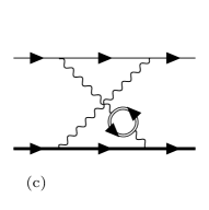
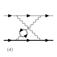


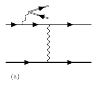
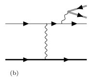
We detail below the content of the three contributions of eq. (1):
-
•
, the virtual two-loop contribution, consists of several classes, both factorisable and non-factorisable:
-
1.
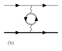
the squared absolute value of the leading-order (LO) amplitude with one-loop photon vacuum polarisation (VP) due to leptons (figure 1 (b));
-
2.
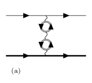
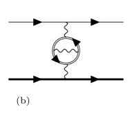
interference between LO diagram and two-loop diagrams with iterated photon VP as well as two-loop irreducible VP (figure 2).
- 3.
-
4.
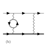
interference between LO diagram and two-loop factorisable contributions where the one-loop diagrams with photonic corrections include a VP insertion in the non-loop photon propagator. Only the two diagrams of figure 4 belong to this class, which exhibits IR divergences. Also for this case the function can be factored out;
-
5.
interference between LO diagram and two-loop irreducible contributions where the one-loop diagrams with photonic corrections include a VP insertion in the loop photon propagator. We have two classes of diagrams:
-
a)
vertex corrections, which are IR safe (figure 5). These diagrams contribute to the NNLO corrections to the QED vertex form factor;
- b)
-
a)
-
1.
-
•
includes the interplay between real photon radiation and leptonic loop insertions, in particular the interference between tree-level diagrams for the process and the same class of diagrams with insertion of the leptonic loop on the virtual photon (figure 7). IR divergences stemming from this set of corrections are cancelled by a sub-set of the contributions considered in the previous item;
-
•
contains the tree-level amplitudes for the processes , with . The production of the pair is forbidden by the available centre of mass energy in the MUonE experiment. We have three different gauge-invariant classes:
-
1.
lepton-pair production through photon radiation from the electron line (figure 8 (a) and (b)),
-
2.
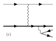
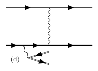
lepton-pair production through photon radiation from the muon line (figure 8 (c) and (d)) and
-
3.
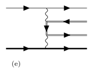
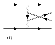
peripheral diagrams, depicted in figure 8 (e) and (f), where the additional leptonic pair originates from the virtual photon propagator 444The plots displayed in figures 8 do not include the diagrams obtained through exchange of identical electrons or muons, which are, however, included in the calculation..
-
1.
The real-pair radiation contribution is particularly important for two reasons: on the pure phenomenological side, when two final state particles escape the MUonE acceptance, the 4-fermion final state mimics a signal event and therefore its contribution is a reducible background and has to be thoroughly investigated under typical MUonE running conditions. On the other side, the interference between different real pair radiation diagrams is expected to give a partial cancellation with its virtual counterpart. For instance, it is known from the literature on Bhabha scattering Jadach:1992nk ; Jadach:1993wk ; Arbuzov:1995cn ; Arbuzov:1995vj ; Jadach:1996ca ; Montagna:1998vb ; Montagna:1999eu ; CarloniCalame:2011zq that the interference between diagrams (a) and (b) of figure 8, once integrated over the phase space available to the electronic pair, develops a term proportional to , which cancels when added to the virtual contribution originating from diagram (a) of figure 5. Similar partial cancellations are expected between virtual contributions and the interference between the diagrams corresponding to the cut of the closed leptonic loop. Moreover, a careful study of the impact of the peripheral diagrams is necessary in view of their potentially large contribution, as will be discussed in the following sections.
3 Calculation of virtual and real-virtual corrections
We build our NNLO virtual leptonic corrections by means of dispersion relation (DR) techniques, starting from the available NLO calculation implemented in Mesmer. According to refs. Hoang:1995ex ; Actis:2007fs ; Actis:2008sk ; Kuhn:2008zs , and the seminal work of refs. Barbieri:1972as ; Barbieri:1972hn , an amplitude involving a photon in a loop with a VP insertion, due to lepton , is obtained by replacing the photon propagator as follows
| (5) |
where the renormalised VP function is obtained from its imaginary part by means of the subtracted DR
| (6) |
with
| (7) | |||||
| (8) |
representing the mass of the lepton circulating in the loop. Since the term in eq. (5) does not contribute because of gauge invariance, the two-loop calculation can be performed starting from the one-loop amplitude with the replacement
| (9) |
The above approach has been used in ref. Actis:2007fs ; Actis:2008sk ; Kuhn:2008zs ; CarloniCalame:2011zq for the calculation of two-loop QED hadronic and leptonic corrections to Bhabha scattering. More recently the same technique has been used in refs. Fael:2018dmz ; Fael:2019nsf to calculate the NNLO hadronic corrections to scattering in the context of the MUonE experiment. Partial preliminary results on NNLO virtual leptonic corrections to muon-electron scattering have been obtained in ref. Balzani:2020 .
Equation (9) leads in a natural way to perform a MC integration in , for the evaluation of NNLO virtual pair corrections, starting from the NLO calculation. Indeed, by exchanging the order of integration variables between the loop momentum and the effective photon mass given by the DR, the one-loop amplitude can be convoluted with a kernel function to obtain the two-loop amplitude with the VP insertion in the following way
| (10) |
where represents the one-loop amplitude with the mass of the virtual photon, where the VP is inserted, set to .
In this way the CPU load for the two-loop calculation remains of the same order of the one-loop calculation, having only one additional dimension in the MC integration. An important point to be checked is the numerical stability of the algorithm. For this reason we performed several internal checks on the convergence of the MC error estimate and cross checks with available analytic expressions, which we document below.
4 Calculation of real corrections
The calculation of the differential and integrated cross sections for real pair emission, i.e. for the processes , with (the case is not allowed at MUonE by energy conservation) is a standard tree-level calculation for processes. Because of the presence of the small electron mass scale and the need of covering the full available phase space in the simulation, the matrix elements have to be computed in a numerically stable way and the numerical integration has to be performed with dedicated samplings, in particular for the final state with electronic pair. As will be discussed later, also the scattering amplitudes for the processes with has been calculated.
The matrix elements (considering only QED interactions) have been calculated with the help of the symbolic manipulation program Form Vermaseren:2000nd ; Kuipers:2012rf ; Ruijl:2017dtg and cross-checked with the automatic package Recola Actis:2016mpe ; Denner:2017wsf , finding perfect agreement (typically the numerical relative difference is at the level and never worse than ) 555In order to select subsets of gauge invariant classes of diagrams, for the calculation of the amplitude with with Recola, we used the rescaling factors and for the and couplings, respectively..
The phase space integration has been carried out with two independent implementations. For both of them the final state momenta are generated in the centre of mass frame and boosted in the laboratory frame. According to one implementation, the 4-body Lorentz invariant phase space
| (11) |
is decomposed into different parameterisations. The diagrams (a) and (b) of figure 8, with the lepton pair radiated from the electron line, require the following parameterisation:
| (12) |
where is the total initial state momentum (with and being the initial muon and electron momenta, respectively), is the -body phase space element
| (13) |
and , , and are the final state muon, electron and , momenta, respectively. In order to obtain reliable numerical MC predictions, different sets of independent variable mappings are necessary to tailor the generation according to the peaking behaviour of diagrams (a) and (b) of figure 8. In particular, for diagram (a) the following set of independent variables is used:
| (14) |
where and are generated in the rest-frame of the pair , and and are the polar and azimuthal angles of the pair momentum in the centre of mass frame. For diagram (b), and are understood in the centre of mass frame with -axis oriented along the outgoing electron . The diagrams (c) and (d) of figure 8, with the lepton pair radiated from the muon line, do not require dedicated parameterisation because is of the same order of magnitude of and therefore the logarithmic structure developed by the numerical integration is not leading. The peripheral diagrams (e) and (f) of figure 8 require a different phase space parameterisation Berends:1994pv ; Kersevan:2004yh :
| (15) | |||||
The independent variables are the invariant masses
| (16) |
and the angles
| (17) |
where , are generated in the rest-frame and and are generated in the rest-frame.
When the pair is an electron-positron pair , all the necessary simmetrised channels with and exchanged are considered.
A second (and independent) phase-space decomposition has been implemented, which is the one used in the official release of Mesmer. In this case, in the principal integration channel, the independent variables are
| (18) |
where , , , is the azimuthal angle in the rest frame, and are the angles in the rest frame, and and are the angles in the rest frame. The importance sampling of the variables in eq. 18 follows as close as possible the peaking structure of the differential cross section, and multi-channel techniques are used to map different structures. For instance, in the case of an extra electronic pair and referring to figure 8, in the principal channel, while , and are sampled uniformly, is sampled as to follow the singularity due to the internal fermion propagator of diagram (b), is sampled according to to flatten the peaks of the photon propagator exchanged between the muon and electron lines and is sampled following . The cosine is distributed according to or , where () is the speed of () in the rest frame, to flatten the peaks due to the internal electron propagator of diagram (a) or the photon propagator in diagram (e). Finally, is sampled according to or , where () is the speed of () in the rest frame, to flatten the peak due to the electron propagator in diagrams (e) and (f). In the other channel, the roles of and are interchanged with and . For identical particles, a symmetrisation of the channels is performed by exchanging .
5 Numerical results
We are going to study the numerical impact of QED NNLO leptonic pair corrections to observables for virtual and real corrections separately, in order to understand the features and the size of each contribution.
The simulations are performed assuming a muon beam 666Lately, it became more likely that MUonE running conditions will use a muon beam. Here we still use a energy for direct comparison with past phenomenological results and because it does not change our conclusions. and according to the following event selection criteria 777It corresponds to Setup 1 in ref. CarloniCalame:2020yoz and to Setup 2 in ref. Alacevich:2018vez . In the latter, also setups with GeV were considered, which are disregarded here for the sake of brevity.:
-
•
and GeV.
The angular cuts model the typical acceptance conditions of the experiment and the electron energy threshold is chosen in order to single out a region where the signal of the experiment is not negligible.
We remark that this event selection is driven by the kinematics and can be rephrased differently to describe the events more in detail. In the kinematics, the outgoing muon is characterised by an angle and, for a incident muon, an energy 888It corresponds to the laboratory energy of a muon scattered backward in the centre-of-mass frame.. When we consider real lepton pair radiation we can have more charged tracks in the detector 999In its present proposal, MUonE will not distinguish positive from negative charges. and therefore we need to introduce a more general event selection inspired by the one of the elastic process. In particular, we can define a muon-like track, characterised by angle lower than and energy larger than , and an electron-like track, with angle lower than and energy larger than . The generalised selection criteria can be defined as follows:
-
•
two tracks in the detector, one muon-like ( and ) and one electron-like ( and )
This alternative definition will be used in the following when 4-body final states are studied, and we will name it basic acceptance cuts.
On top of it, we are going to consider also three extra selection cuts (and combinations of them), which are tailored to select elastic events in order to suppress reducible backgrounds and keep the sensitivity to the signal. The elasticity cuts we implement are:
-
1.
cut 1 an additional cut on the minimum electron- and muon-like scattering angles, , to reduce the impact of peripheral diagrams in events with additional electron pair emission. For illustrative purposes, we use the value , which appears to be a good compromise between the requirement of keeping sensitivity to in the large region 101010We remind the reader that the largest sensitivity occurs for mrad (see figure 13 of ref. Alacevich:2018vez ). and effectively suppressing the reducible background;
-
2.
cut 2 acoplanarity cut 111111The value is chosen in analogy with refs. Alacevich:2018vez ; CarloniCalame:2020yoz and perhaps it is too small for MUonE running conditions., where are the azimuthal angles of the electron- and muon-like momenta;
-
3.
cut 3 elasticity distance , where is defined as the minimal Cartesian distance of the , point in the - plane from the elastic curve. The elastic curve can be parameterised by the function
(19) where is defined in eq. (9) of ref. Abbiendi:2016xup and is the incident muon energy in the laboratory reference frame. The distance of the generic point is defined as
(20) While the optimal value for can be determined only with a realistic simulation that takes into account of all the experimental conditions and detector effects, we use for the present study the reference value mrad.
When considering the emission of real leptonic pairs in the following, in order to study the effects from different gauge invariant contributions and their interplay with the virtual corrections from a purely theoretical point of view, neglecting the effect of identical particles, we will begin our analysis considering the processes for the two cases and . The three gauge invariant contributions are the radiation from the electron line, from the muon line and the two peripheral diagrams, according to the discussion of section 2 on the ingredients of . In this exercise we are completely inclusive over the additional “” pair and assume the cuts are applied to the final state electron and muon, as if they were distinguishable from the extra leptons in the final state (asymmetric cuts). The obtained numerical results must be considered “academic” since the event selection does not fully match the realistic MUonE experimental settings.
As a second step, we consider the true processes and , taking into account more realistic conditions. In MUonE the final state charged particles are detected through their tracks in the silicon detectors, without charge identification. We therefore require that exactly two tracks are reconstructed in the detector by asking that they have a threshold energy larger than GeV and an angle lower than mrad. If more than two tracks are reconstructed, the event is rejected. Otherwise, of the two selected tracks, we require one to be muon-like and the other to be electron-like, as per definitions above. We will further show the effects of cutting through cut 1-3. We remark that in principle any pair combination of final state leptons can fall within the only-two-tracks criterium, but we verified a posteriori that the final state muon of the process is always the muon-like track.
The input parameters for the simulations are set to
If is the incoming muon (electron) momentum and is the muon(electron)-like outgoing momentum 121212We notice that, when considering the emission of an extra real electronic pair, can be any of the final state or the momentum, according to which one represents the electron-like track., the considered differential observables are the following ones:
| (21) |
where , , and are the scattering angles, in the laboratory frame, of the outgoing electron- and muon-like tracks, respectively.
We decide to represent the corrections as a differential factor defined by
| (22) |
i.e. we normalise the differential cross sections under study w.r.t. the LO ones. The choice is dictated by consistency and for direct comparison with results presented in refs. Alacevich:2018vez ; CarloniCalame:2020yoz and because the 10ppm accuracy goal is implicitly referred to LO results.
We notice that in the following we show also the hadronic effects already considered in Fael:2019nsf , for completeness and cross-check purposes.
5.1 NNLO virtual pair corrections: the factorised diagrams
In this section we show the impact of NNLO virtual pair corrections of figures 1 and 2 131313Despite they are calculated in the MC code, here we do not show any effect due to or top quark loops because they are small on the scale of the effects induced by , or hadronic loops., which are factorised over the tree-level cross section and contribute to the running of the electromagnetic coupling constant.
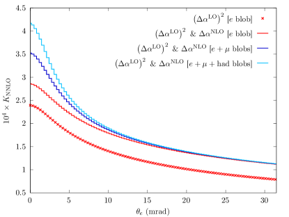
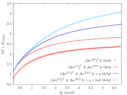
In figure 9, the red histograms show the contribution of the electron circulating in the loop on the (left) and (right) distributions. The points stand for the term and solid lines include also the term . The first term is positive and ranges from about for zero electron scattering angle to about at mrad. As expected, the range of the corrections on is the same with opposite slope w.r.t. the electron angle, with the muon angle ranging from lower to higher angles. The irreducible diagram of figure 2 (b) gives a positive shift, almost flat over the whole range of about . The blue solid line includes also the two-loop contribution with the muon circulating in the loops. It is a negligible contribution for mrad ( mrad) and becomes of the order of for mrad , where the exchanged increases in absolute value. The light blue solid line includes all the leptonic contributions and the hadronic corrections, calculated with the help of the routines of the KNT v3.0.1 package Keshavarzi:2018mgv 141414Available upon request from the authors. Detailed cross-checks with the hadr5x19.f routine by Fred Jegerlehner (available at www-com.physik.hu-berlin.de/~fjeger/software.html, see ref. Jegerlehner:2018zrj ) have been carried out, finding fully compatible results.. The latter contribution is similar in shape and size to the one of the muon loop.
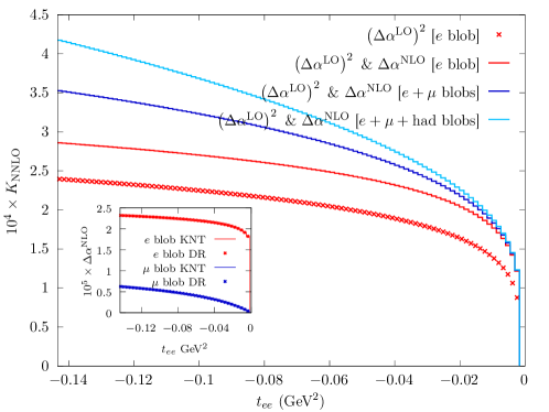
The same breakdown of the separate effects, displayed in incremental way, is shown for the distribution in figure 10. For comparison purposes, in the inset we present the function for an electron or muon loop as coded in the KNT v3.0.1 package and as obtained through a DR, showing perfect agreement. The DR we use here is fully analogous to eq. (6) where the function is replaced by the NLO function resulting from the QED limit of eq. (18) in ref. Harlander:2002ur .
5.2 Vacuum polarisation on photonic vertex corrections
Among the two-loop irreducible contributions where the one-loop diagrams with photonic corrections include a VP insertion in the loop photon propagator, the diagrams of figure 5, together with their respective counterterms, are gauge-invariant and IR safe. Therefore it is meaningful to investigate their numerical relevance. In figures 11 and 12 we show, separately, all the effects of different leptons (electron and muon) in the photonic vertex one-loop diagrams of figure 5 for the three observables , , . For each contribution the histogram refers to the calculation through DR and the points refer to the analytical calculation. For the case of a closed loop with a lepton with mass equal to the one of the current which the photon loop is attached to, the analytical calculation presented in Appendix A.2 of ref. Bonciani:2004gi has been used. In all other cases (i.e. mass of the lepton flowing in the VP insertion different from the mass of the lepton of the external current), we use an in-house independent calculation which is described in Appendix A.
We would like to remark that for all cases excellent numerical agreement is found, which indicates also that the DR approach is implemented correctly.
From the phenomenological point of view, the largest contribution is given, as expected, by the electron loop on the electron line (red curves), which reaches the level of at the kinematical boundaries corresponding to the maximum . As known in the literature, see e.g. refs. Burgers:1985qg ; Arbuzov:1995vj ; Bonciani:2004gi , the leading logarithmic term of the electron loop in the vertex correction on the electron line is proportional to which is expected to be partially cancelled by the corrections corresponding to the real emission of an pair. This will be discussed in the following section with a numerical investigation.
The electron loop on the muon line is suppressed w.r.t. the previous contribution and reaches the level of at the kinematical boundary. The smallest contribution is given by the muon loop on the muon line, which never reaches the level.
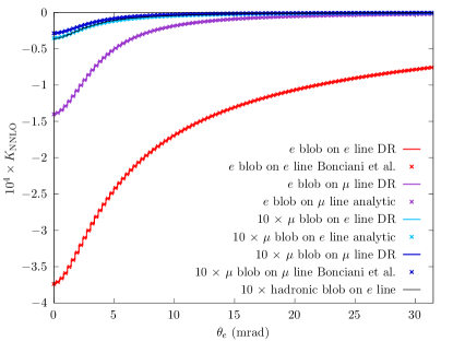
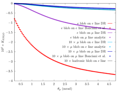
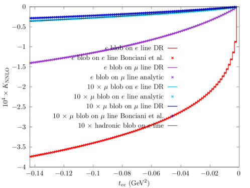
Finally, the muon loop correction on the electron line is of the same size of the hadronic correction on the electron line, remaining at most at the level of a few ppm.
5.3 NNLO virtual pair corrections: the complete set of diagrams
In this subsection we present the numerical impact of the contributions due to the photonic one-loop amplitudes (virtual and real contributions) with an additional closed leptonic loop, namely the sum of the interference between the diagram in figure 1 (a) with the diagrams in figures 4, 5 and 6 plus the interference of the diagram in figure 1 (b) with the diagrams in figure 3. Also real radiation is added (i.e. the interference of the diagrams in figure 7 with the very same diagrams without loop insertion), as well as all the contributions described in sections 5.1 and 5.2. As we know from previous studies on NLO Alacevich:2018vez and NNLO photonic CarloniCalame:2020yoz (and also hadronic Fael:2019nsf ) corrections, the real radiation can give large contributions, in particular for the electron scattering angle distribution. For this reason in refs. Alacevich:2018vez ; CarloniCalame:2020yoz the additional acoplanarity cut (cut 2 as defined in the introduction to this section) was introduced, in order to partially remove hard radiation effects.
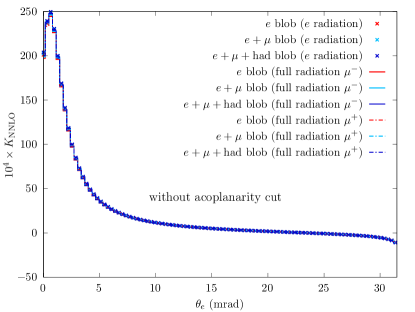
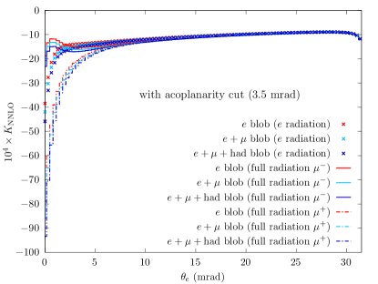
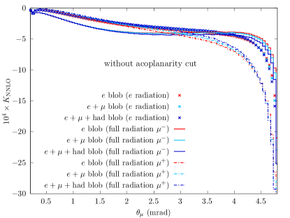
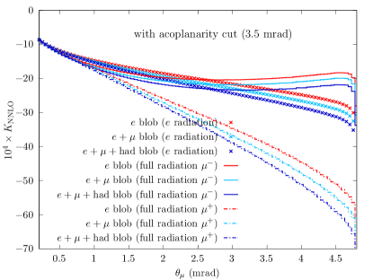
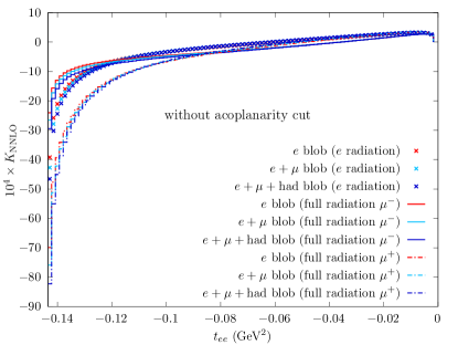
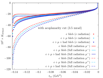
Figure 13 shows the impact of the virtual pair corrections on the electron scattering angle distribution for different levels of approximation: radiation from the electron leg only or the complete calculation for or beam. For each of these cases, three different contributions are considered: only electron loop, electron plus muon loop and electron plus muon plus hadronic loop. On the left, in the absence of any acoplanarity cut, all the above described contributions are almost degenerate, with very large corrections up to about for small scattering angles, driven by the electron loop on top of radiation from the electron line. On the right, the additional acoplanarity cut changes the sign of the corrections, which range from about for large scattering angles to several for . In particular, the contribution from the electron line radiation reaches the value of about , driven by the electron closed loop. The muon and the hadronic loops are of the same order of a few . The full corrections (solid lines for beam and dot-dashed line for beam) display a difference with respect to the radiation from the electron line at the few 0.1% level for small scattering angles.
Figure 14 shows the impact of the virtual pair corrections on the muon angle distribution 151515In this case and similarly thorough the rest of the paper, we do not show muon scattering angles because the corrections are huge and would spoil the readability of the plots. The reason for this feature is that the LO prediction becomes tiny in the angular range below , as a consequence of the applied acceptance cuts, while 3-body (and later 4-body) events populate the region, not being constrained by the kinematics.. In this case, the corrections grow to dozens of as reaches its maximum. We notice a flattening of the factor when the acoplanarity cut is added (right). The effect is generally dominated by electron loop insertion, and in the full calculation corrections for an incident or are opposite with respect to corrections on the electron line only. Finally, figure 15 shows the impact on the momentum transfer , where similar considerations apply.
We conclude the section by remarking that the application of extra elasticity cuts, in particular cut 1+3, does not change the overall effects and size of the corrections considered here. In contrast, they have a much more dramatic effect in reducing the reducible background due to real electron pair emission, as will be discussed in the following section 5.5.
5.4 NNLO real pair corrections, asymmetric event selection (academic case)
In this section we present the impact of the emission of a real leptonic pair, treated in an inclusive way (i.e. with asymmetric cuts). To exclude diagrams with the exchange of identical particles, we consider in this section the processes , setting , and adopt the generalised event selection criteria described in the introduction of this section. At the end of this subsection, for completeness, we consider also the negligible contribution due to the emission of an extra muon pair ().
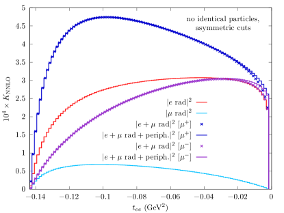
In the left panel of figure 16 we show the contribution of the “” pair (with ) on the distribution. Three different gauge invariant classes of diagrams are considered: radiation from the electron line only (red line), radiation from the muon line only (light-blue line), radiation from both electron and muon lines (see figure 8 (a)-(d)), including their interferences but neglecting the peripheral diagrams (figure 8 (e) and (f)). For the latter two options, the blue and violet crosses refer to the and beam cases, respectively. The results obtained with the complete matrix elements, including also the peripheral diagrams, are displayed with the blue and violet line for the and beam, respectively. As a general comment we can see that the numerical impact of the real radiation, on the distribution, is at the level of few , with dominance of the radiation from the electron line w.r.t. the radiation from the muon line. The interference between the radiation from the electron and muon lines is of different sign when flipping the charge of the incoming muon, as already seen for the QED NLO corrections in ref. Alacevich:2018vez . The effect of the peripheral diagrams is almost negligible.
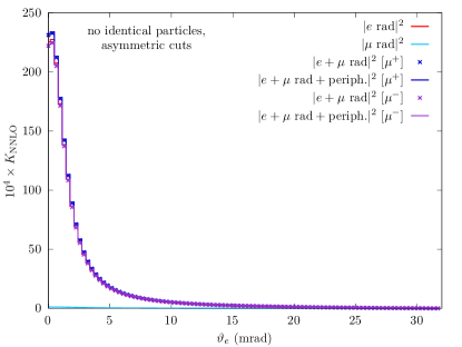
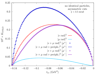
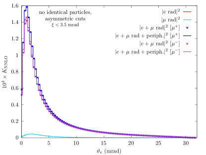
The right panel of figure 16 shows the electron scattering angle distribution, normalised to the LO prediction, where the large correction factor for the radiation from the electron line is clearly visible for , analogously to what happens for the NLO QED correction. As commented in ref. Alacevich:2018vez , the effect is in part due to the vanishing of the LO differential cross section as . For this reason, in ref. Alacevich:2018vez the acoplanarity cut has been introduced, which allows to partially remove the enhancements. Applying the same acoplanarity cut on our signature, for the observable we obtain the results displayed in the left panel of figure 17, where the maximum of the correction is reduced to about , for the case of an incoming beam. The corresponding corrections on the observable are shown in the left panel of figure 17, and also here we remark the large suppression factor induced by the acoplanarity cut.
Within this case, where we academically suppose one final state electron to be distinguishable from those of the extra pairs, the contribution from the peripheral diagrams is almost negligible for all the considered observables.
We also notice that on the factor for the distribution, in the most inclusive case, without the acoplanarity cut, corrections due to the emission of an extra pair are positive and of the same order of magnitude as the negative corrections due to VP insertion on photonic vertex corrections, discussed in section 5.2. We see indeed a partial cancellation between real and virtual pair corrections, for this subset of contributions.
Before considering also identical particles and fully realistic event selection on real pair emission, we show in this academic case the impact of events (i.e. with ) on the distribution, for completeness.
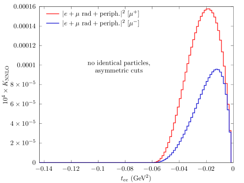
It is clear from figure 18, where the red curve shows the incoming case and the blue one the incoming case, that this process gives a totally negligible contribution, reaching at maximum a few units in w.r.t. the LO differential cross section. We also notice that below there are no events because of phase space constraints 161616On the same grounds, we expect charged pion pair emission () to be even more suppressed due to the further reduction of available phase space because of the larger pion mass..
5.5 NNLO real pair corrections, realistic event selection
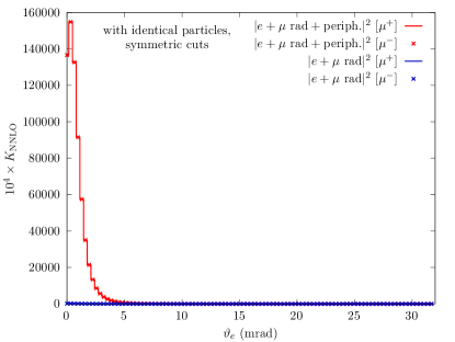
The discussion on real electron pair radiation of section 5.4 shows the relevance of real pair emission in the NNLO complete calculation. However, those results are purely academic since the analysis is completely inclusive on the emitted electron pair and does not take into account the MUonE realistic event selection, where the four final state leptons can produce up to four tracks in the detector. According to the discussion of section 5, to mimic an elastic event, we can require that only two tracks (one muon-like, one electron-like) are seen in the detector. In this way, without charge identification, in principle every pair out of the six possible pairings can hit the detector while the remaining two particles are below energy threshold and/or out of the angular allowed range. This requires the use of the full matrix elements for the calculation of the cross sections of the processes (with MUonE realistic event selection we are considering here, no events for the process satisfy the criteria, because at least three charged visible particles are always present), including all the diagrams with the two indistinguishable electrons interchanged, which were neglected in the previous subsection, and the adoption of symmetric cuts that do not distinguish identical particles in the final state.
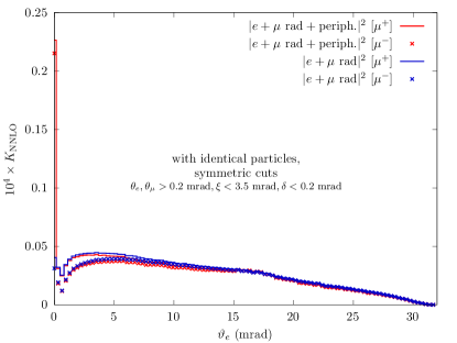
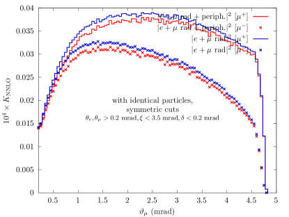
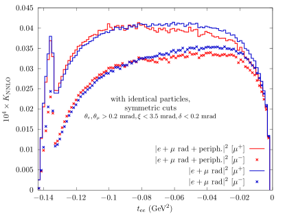
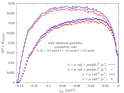
This introduces a new important feature: there is no distinction between the electron of the underlying tree-level and the electron or positron of the emitted pair. As a consequence, in the photon propagators the exchanged momentum can become very close to zero, giving a dramatic enhancement in the cross section and in the distributions, especially at the corner of the phase space. In this enhancement the peripheral diagrams (figures 8 (e)-(f)) give by far the largest contribution. For instance, a sharp peak in a very small window of the scattering angles can be seen in figure 19, where it is evident that “switching-on” peripheral diagrams produces a huge effect.
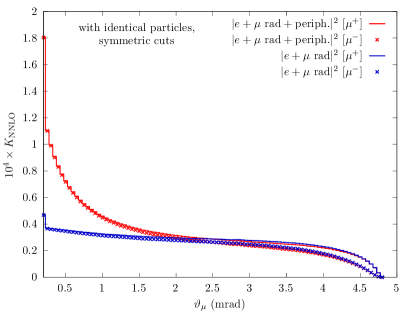
The kinematical configurations related to these enhancements correspond typically to small momentum transfer for or (figure 20) and could spoil the sensitivity of MUonE to the hadronic component of the QED running coupling constant by distorting in a significant way the differential cross sections where the signal to be measured is more important.
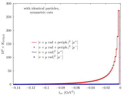
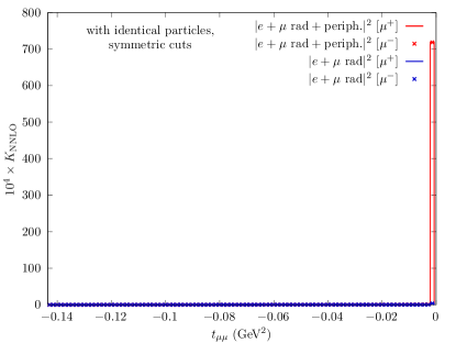
Even with the inclusion of the acoplanarity cut, the numerical impact of real pair radiation remains at the level of , with a large contribution for reaching the level, as can be seen in figure 21.
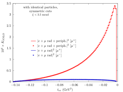
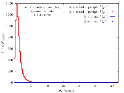
In order to reduce the impact of real pair radiation to a manageable level, we propose to further filter events through the cuts labelled as cut 1-3 and described in the introduction to section 5. The effectiveness of the additional cuts in suppressing real electron pair radiation events can be visualised with the scatter plot of the - angles correlation displayed in figure 22.
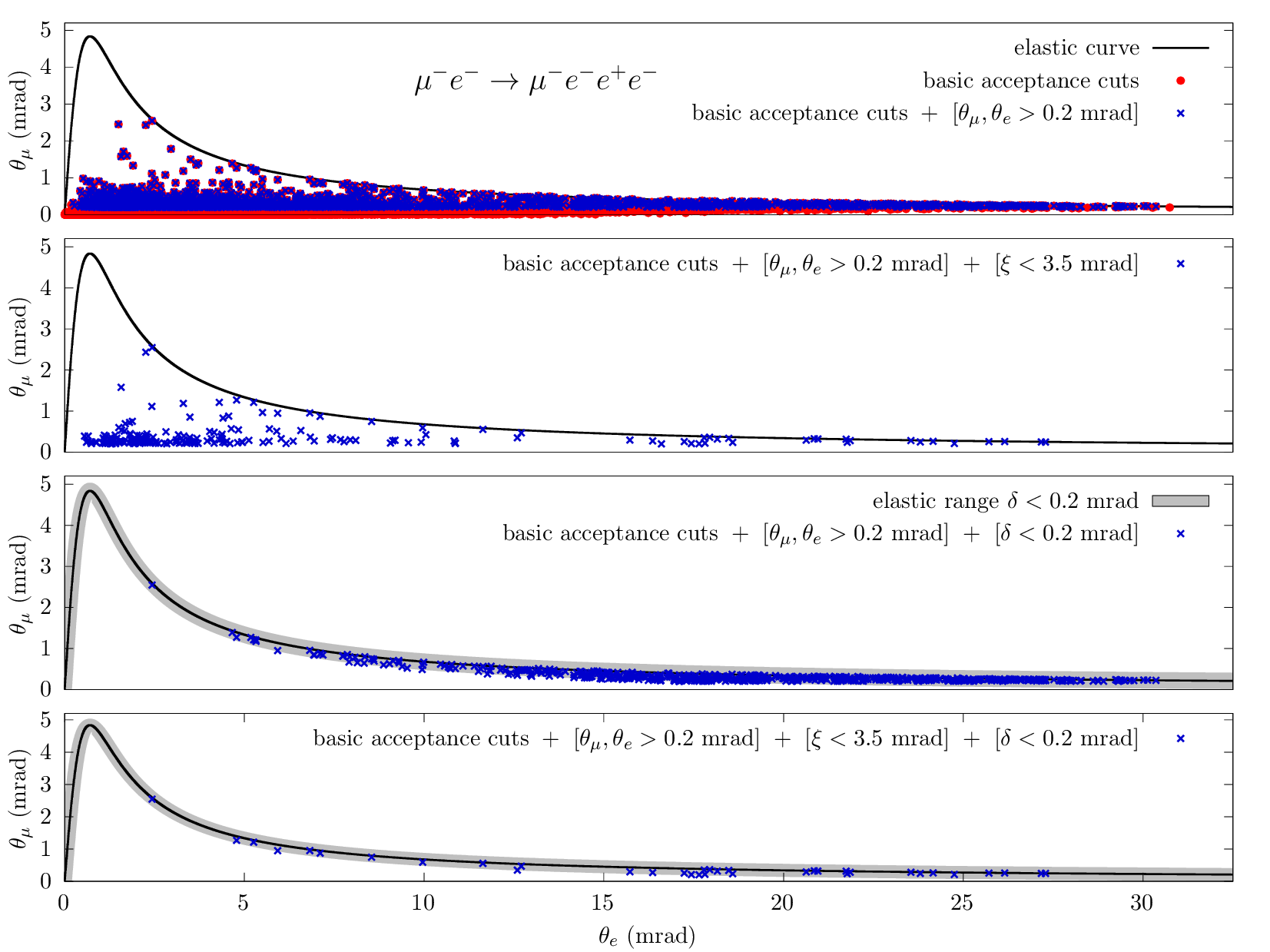
The upper panel shows, with red points, the scatter distribution of the coordinates for a sample of events for the process with only one muon-like and one electron-like track. It is clearly seen that many points fall well outside the elastic correlation curve (black line), in particular they gather in the region of small and . The blue crosses display the same sample after applying the additional cut (cut 1). It is clearly visible the removal of the events with close to 0. The background rejection efficiency of such a cut is of about . In the second panel from the top, the effect of adding the acoplanarity cut (cut 1+2) is shown and the rejection efficiency increases to about . The third panel from the top displays the effect of imposing the cut on the distance from the elasticity correlation curve, , on top of cut 1. In this case the rejection efficiency is at the level of . Finally, the bottom panel shows the effects of combining the three cuts (cut 1+2+3). As can be seen, this combination is particularly effective in reducing the real electron pair production, since only a tiny fraction (as small as ) of background events passes through the selection. It is interesting to observe the complementarity between the and cuts. The latter alone suppresses hard radiation contributions while allowing for a certain degree of acoplanarity between the azimuthal angles of the two final state tracks, due to soft transverse radiation.
This analysis allows us to propose an improved event selection, cut 1-3, as defined in section 5 for the analysis of MUonE data. As can be seen in figures 23 and 24, with this event selection the real emission contribution gets reduced to the ppm level over the full kinematical range. It is worth noticing, for instance in the factor, a peak on the leftmost bin: it can be traced back to few events that, after applying cut 1+2, lie in the region allowed by the elasticity cut.
It is understood that more complete simulations will be needed to select the optimum values for the cut parameters , and . Here, we have only demonstrated that by a sensible choice of the cut parameters the potentially large background due to electron-pair emission can be reduced at the level.
6 Summary and prospects
In this work we have discussed the calculation of the NNLO leptonic corrections to processes and their implementation into the Monte Carlo code Mesmer, used for simulations for the MUonE experimental proposal. Such a project aims at a high precision measurement of the effective QED coupling constant in the space-like region, which will allow for a determination of the leading order hadronic contribution to the muon anomaly, in a way completely independent from time-like dispersion relation and Lattice QCD approaches.
The NNLO leptonic corrections consist of virtual and real contributions. The former have been calculated with dispersion relation techniques including all finite mass effects. For the class of vertex corrections, the numerical results have been cross-checked with exact analytical formulae, valid for arbitrary internal and external masses, finding excellent agreement. Also the hadronic contributions have been included by means of two different parameterisations existing in the literature. The real corrections have been calculated by means of exact matrix elements, taking into account all finite mass effects.
On the phenomenological side, we analysed all different, gauge-invariant, classes of virtual contributions, investigating their numerical impact on the differential observables relevant for MUonE realistic running conditions. As expected, the leading contributions come from the closed electron loop diagrams and the overall size of the factorised and vertex contributions is of the order of few (positive the former, negative the latter). The vacuum polarisation insertions on the NLO QED photonic corrections can reach the level of few , with shapes driven by the NLO photonic corrections. The corrections are negative for all distributions, except for the electron scattering angle distribution, where they become positive, reaching the few level for . Similarly to what happens to the large QED NLO correction to , the introduction of the acoplanarity cut mitigates the effects and brings the corrections to negative values. On the other hand the acoplanarity cut enhances the size of the corrections of IR origin.
The hadronic contributions are of the same order of magnitude of the muon loop insertions, as already noticed in previous studies on Bhabbha scattering at flavour factories.
Particular attention has been paid to the real leptonic pair emission. Because of the low centre of mass energy combined with realistic event selection criteria, the pairs do not play almost any role at MUonE. On the other hand, the emission of pairs is particularly important. In general the processes are distinguishable from the elastic processes. However, under realistic MUonE event selections, the processes can produce only two charged tracks in the final state and become, therefore, degenerate with the elastic signal events. In this case the real pair emission cross section has to be summed to the virtual pair emission contribution, to reach a reliable theoretical prediction. Because of the presence of two indistinguishable electrons and peripheral diagrams, we observed very large positive contributions for small and as well as for small and values, which are not tamed by the previously introduced acoplanarity cut. In order to control these effects we studied a combination of additional cuts, namely a small minimum scattering angle for the two observed tracks and a maximum distance from the elasticity correlation curve . After considering all the above cuts, the size of the real pair radiation effects has been shown to remain below the level.
Therefore, the combined effects of virtual and real pair radiation under the simplified event selection we considered are dominated by virtual contributions, in particular the ones stemming from electron loops, which, depending on the observable, can reach the level in units of the LO differential cross sections. It is true that there is a partial cancellation between a subset of the virtual and a subset of the real contributions, but the presence of peripheral diagrams in real pair emission spoils the expected cancellation and forces the introduction of elasticity cuts to keep under control a potentially large background to the signal.
The work presented in this paper represents an additional step towards the implementation of a fully fledged MC generator including the complete set of NNLO QED corrections matched to multiple photon emission, which will be ultimately needed for the analysis of MUonE data.
Acknowledgements.
We are sincerely grateful to all our MUonE colleagues for stimulating collaboration and many useful discussions, which are the framework of the present study. We are particularly indebted to Giovanni Abbiendi, Matteo Fael, Pierpaolo Mastrolia and Massimo Passera for carefully reading the manuscript and for useful feedback. One of the authors would like to thank Dr. Ulrich Schubert for useful discussions.Appendix A Master Integrals for vertex corrections
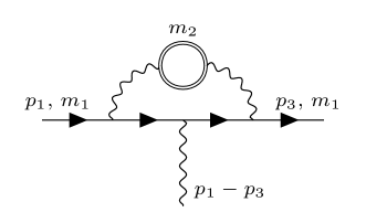
The computation of the Feynman diagrams in figure 5 is obtained by calculating the vertex form factors of the generic diagram shown in figure 25, where is the external lepton mass, whereas represents the lepton loop mass. For the simpler case of , there are known results in literature Bonciani:2003cj ; Bonciani:2003te that can be used. However, to the best of our knowledge, the complete analytic expression for the case without any expansion in the mass ratio is not yet available. In this section we show a way to calculate these vertex form factors for .
The kinematics of the process is given by
| (23) |
The integrals that appear in the calculation are of the form
| (24) |
where is a normalisation factor:
| (25) |
The propagators are defined as:
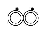
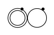
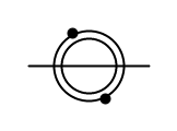
Seven master integrals, depicted in figure 26, are necessary to calculate the form factors. We solved these particular integrals using differential equation methods Kotikov:1990kg ; Remiddi:1997ny ; Gehrmann:1999as : we chose a suitable basis of master integrals, such that the dimensional regularisation parameter factorises from the kinematics. The integrals were then encoded in a -form, also called canonical form Henn:2013pwa , which we were able to obtain using the Magnus algorithm DiVita:2014pza ; Argeri:2014qva . The kinematic variables were chosen in such a way that the arguments of the ’s were simple rational functions, which enabled us to express the integrals in terms of the generalised polylogarithms Remiddi:1999ew ; Gehrmann:2001jv ; Vollinga:2004sn . The master integrals were then calculated up to required expansion to determine the form factor: they are , , , , , and , which can be found in the ancillary file in the arXiv version of the paper. Here we explicitly write the first four master integrals up to finite term to show the used convention.
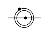
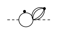
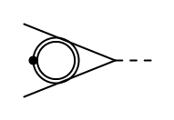
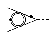
| (26) | ||||
| (27) | ||||
| (28) | ||||
| (29) |
We introduced the dimensionless variables and such that the arguments of the were simple rational functions:
| (30) |
The following equations show the solutions that are suitable for the region of interest:
| (31) |
Throughout the form factor calculation, the Integration by Parts reduction Tkachov:1981wb ; Chetyrkin:1981qh ; Laporta:2001dd was carried out using the publicly available codes Reduze vonManteuffel:2012np and FIRE Smirnov:2019qkx . The differential equations were generated using Reduze and, to rationalise the arguments of the , we used the package RationalizeRoots Besier:2019kco . The numerical validations were accomplished using SecDec Borowka:2015mxa and the numerical evaluation of generalised polylogs was performed with GiNaC Vollinga:2004sn and handyG Naterop:2019xaf . A detailed result of the vertex form factor is presented in ref. Syed:2021nc .
References
- (1) Muon g-2 collaboration, Measurement of the Positive Muon Anomalous Magnetic Moment to 0.46 ppm, Phys. Rev. Lett. 126 (2021) 141801 [2104.03281].
- (2) Muon g-2 collaboration, Final Report of the Muon E821 Anomalous Magnetic Moment Measurement at BNL, Phys. Rev. D73 (2006) 072003 [hep-ex/0602035].
- (3) F. Jegerlehner and A. Nyffeler, The Muon g-2, Phys. Rept. 477 (2009) 1 [0902.3360].
- (4) F. Jegerlehner, The Anomalous Magnetic Moment of the Muon, Springer Tracts Mod. Phys. 274 (2017) pp. 1.
- (5) T. Aoyama et al., The anomalous magnetic moment of the muon in the Standard Model, Phys. Rept. 887 (2020) 1 [2006.04822].
- (6) Fermilab E989 collaboration, The New Muon g-2 experiment at Fermilab, Nucl. Part. Phys. Proc. 273-275 (2016) 584 [1411.2555].
- (7) Muon g-2 collaboration, Muon (g-2) Technical Design Report, 1501.06858.
- (8) J-PARC muon g-2/EDM collaboration, New approach to the muon g-2 and EDM experiment at J-PARC, J. Phys. Conf. Ser. 295 (2011) 012032.
- (9) J-PARC g-2 collaboration, Measurement of muon g-2 and EDM with an ultra-cold muon beam at J-PARC, Nucl. Phys. Proc. Suppl. 218 (2011) 242.
- (10) E.-H. Chao, A. Gérardin, J.R. Green, R.J. Hudspith and H.B. Meyer, Hadronic light-by-light contribution to from lattice QCD with SU(3) flavor symmetry, Eur. Phys. J. C 80 (2020) 869 [2006.16224].
- (11) I. Danilkin, M. Hoferichter and P. Stoffer, A dispersive estimate of scalar contributions to hadronic light-by-light scattering, Phys. Lett. B 820 (2021) 136502 [2105.01666].
- (12) E.-H. Chao, R.J. Hudspith, A. Gérardin, J.R. Green, H.B. Meyer and K. Ottnad, Hadronic light-by-light contribution to from lattice QCD: a complete calculation, Eur. Phys. J. C 81 (2021) 651 [2104.02632].
- (13) F. Jegerlehner, The Muon g-2 in Progress, Acta Phys. Polon. B49 (2018) 1157 [1804.07409].
- (14) A. Keshavarzi, D. Nomura and T. Teubner, The muon and : a new data-based analysis, Phys. Rev. D97 (2018) 114025 [1802.02995].
- (15) M. Davier, A. Hoecker, B. Malaescu and Z. Zhang, A new evaluation of the hadronic vacuum polarisation contributions to the muon anomalous magnetic moment and to , Eur. Phys. J. C 80 (2020) 241 [1908.00921].
- (16) G. Colangelo, M. Hoferichter and P. Stoffer, Constraints on the two-pion contribution to hadronic vacuum polarization, Phys. Lett. B 814 (2021) 136073 [2010.07943].
- (17) M. Benayoun, L. DelBuono and F. Jegerlehner, BHLS2 Upgrade : spectra, muon HVP and the [] System, 2105.13018.
- (18) M. Della Morte, A. Francis, V. Gülpers, G. Herdoiza, G. von Hippel, H. Horch et al., The hadronic vacuum polarization contribution to the muon from lattice QCD, JHEP 10 (2017) 020 [1705.01775].
- (19) Fermilab Lattice, LATTICE-HPQCD, MILC collaboration, Strong-Isospin-Breaking Correction to the Muon Anomalous Magnetic Moment from Lattice QCD at the Physical Point, Phys. Rev. Lett. 120 (2018) 152001 [1710.11212].
- (20) Budapest-Marseille-Wuppertal collaboration, Hadronic vacuum polarization contribution to the anomalous magnetic moments of leptons from first principles, Phys. Rev. Lett. 121 (2018) 022002 [1711.04980].
- (21) H.B. Meyer and H. Wittig, Lattice QCD and the anomalous magnetic moment of the muon, Prog. Part. Nucl. Phys. 104 (2019) 46 [1807.09370].
- (22) RBC, UKQCD collaboration, Calculation of the hadronic vacuum polarization contribution to the muon anomalous magnetic moment, Phys. Rev. Lett. 121 (2018) 022003 [1801.07224].
- (23) D. Giusti, F. Sanfilippo and S. Simula, Light-quark contribution to the leading hadronic vacuum polarization term of the muon from twisted-mass fermions, Phys. Rev. D 98 (2018) 114504 [1808.00887].
- (24) D. Giusti, V. Lubicz, G. Martinelli, F. Sanfilippo and S. Simula, Electromagnetic and strong isospin-breaking corrections to the muon from Lattice QCD+QED, Phys. Rev. D 99 (2019) 114502 [1901.10462].
- (25) D. Giusti and S. Simula, Lepton anomalous magnetic moments in Lattice QCD+QED, PoS LATTICE2019 (2019) 104 [1910.03874].
- (26) PACS collaboration, Hadronic vacuum polarization contribution to the muon with 2+1 flavor lattice QCD on a larger than (10 fm lattice at the physical point, Phys. Rev. D 100 (2019) 034517 [1902.00885].
- (27) Fermilab Lattice, LATTICE-HPQCD, MILC collaboration, Hadronic-vacuum-polarization contribution to the muon’s anomalous magnetic moment from four-flavor lattice QCD, Phys. Rev. D 101 (2020) 034512 [1902.04223].
- (28) A. Gérardin, M. Cè, G. von Hippel, B. Hörz, H.B. Meyer, D. Mohler et al., The leading hadronic contribution to from lattice QCD with flavours of O() improved Wilson quarks, Phys. Rev. D 100 (2019) 014510 [1904.03120].
- (29) C. Aubin, T. Blum, C. Tu, M. Golterman, C. Jung and S. Peris, Light quark vacuum polarization at the physical point and contribution to the muon , Phys. Rev. D 101 (2020) 014503 [1905.09307].
- (30) D. Giusti and S. Simula, Ratios of the hadronic contributions to the lepton from Lattice QCD+QED simulations, Phys. Rev. D 102 (2020) 054503 [2003.12086].
- (31) C. Lehner and A.S. Meyer, Consistency of hadronic vacuum polarization between lattice QCD and the R-ratio, Phys. Rev. D 101 (2020) 074515 [2003.04177].
- (32) S. Borsanyi et al., Leading hadronic contribution to the muon magnetic moment from lattice QCD, Nature 593 (2021) 51 [2002.12347].
- (33) C.M. Carloni Calame, M. Passera, L. Trentadue and G. Venanzoni, A new approach to evaluate the leading hadronic corrections to the muon -2, Phys. Lett. B746 (2015) 325 [1504.02228].
- (34) B. Lautrup, A. Peterman and E. de Rafael, Recent developments in the comparison between theory and experiments in quantum electrodynamics, Phys. Rept. 3 (1972) 193.
- (35) G. Abbiendi et al., Measuring the leading hadronic contribution to the muon g-2 via scattering, Eur. Phys. J. C77 (2017) 139 [1609.08987].
- (36) A.B. Arbuzov, D. Haidt, C. Matteuzzi, M. Paganoni and L. Trentadue, The Running of the electromagnetic coupling alpha in small angle Bhabha scattering, Eur. Phys. J. C34 (2004) 267 [hep-ph/0402211].
- (37) OPAL collaboration, Measurement of the running of the QED coupling in small-angle Bhabha scattering at LEP, Eur. Phys. J. C45 (2006) 1 [hep-ex/0505072].
- (38) KLOE-2 collaboration, Measurement of the running of the fine structure constant below 1 GeV with the KLOE Detector, Phys. Lett. B 767 (2017) 485 [1609.06631].
- (39) MUonE collaboration, Letter of Intent: the MUonE project, Tech. Rep. CERN-SPSC-2019-026, SPSC-I-252, CERN, Geneva (Jun, 2019).
- (40) G. Abbiendi et al., Results on multiple Coulomb scattering from 12 and 20 GeV electrons on carbon targets, JINST 15 (2020) 01 [1905.11677].
- (41) G. Ballerini et al., A feasibility test run for the MUonE project, Nucl. Instrum. Meth. A 936 (2019) 636.
- (42) G. Abbiendi et al., A study of muon-electron elastic scattering in a test beam, JINST 16 (2021) P06005 [2102.11111].
- (43) P. Banerjee et al., Theory for muon-electron scattering @ 10 ppm: A report of the MUonE theory initiative, Eur. Phys. J. C 80 (2020) 591 [2004.13663].
- (44) M. Alacevich, C.M. Carloni Calame, M. Chiesa, G. Montagna, O. Nicrosini and F. Piccinini, Muon-electron scattering at NLO, JHEP 02 (2019) 155 [1811.06743].
- (45) P. Mastrolia, M. Passera, A. Primo and U. Schubert, Master integrals for the NNLO virtual corrections to scattering in QED: the planar graphs, JHEP 11 (2017) 198 [1709.07435].
- (46) S. Di Vita, S. Laporta, P. Mastrolia, A. Primo and U. Schubert, Master integrals for the NNLO virtual corrections to scattering in QED: the non-planar graphs, JHEP 09 (2018) 016 [1806.08241].
- (47) T. Engel, C. Gnendiger, A. Signer and Y. Ulrich, Small-mass effects in heavy-to-light form factors, JHEP 02 (2019) 118 [1811.06461].
- (48) T. Engel, A. Signer and Y. Ulrich, A subtraction scheme for massive QED, JHEP 01 (2020) 085 [1909.10244].
- (49) C.M. Carloni Calame, M. Chiesa, S.M. Hasan, G. Montagna, O. Nicrosini and F. Piccinini, Towards muon-electron scattering at NNLO, JHEP 11 (2020) 028 [2007.01586].
- (50) P. Banerjee, T. Engel, A. Signer and Y. Ulrich, QED at NNLO with McMule, SciPost Phys. 9 (2020) 027 [2007.01654].
- (51) D.R. Yennie, S.C. Frautschi and H. Suura, The infrared divergence phenomena and high-energy processes, Annals Phys. 13 (1961) 379.
- (52) R. Bonciani et al., The two-loop four-fermion scattering amplitude in QED, 2106.13179.
- (53) M. Fael, Hadronic corrections to - scattering at NNLO with space-like data, JHEP 02 (2019) 027 [1808.08233].
- (54) M. Fael and M. Passera, Muon-Electron Scattering at Next-To-Next-To-Leading Order: The Hadronic Corrections, Phys. Rev. Lett. 122 (2019) 192001 [1901.03106].
- (55) P.S.B. Dev, W. Rodejohann, X.-J. Xu and Y. Zhang, MUonE sensitivity to new physics explanations of the muon anomalous magnetic moment, JHEP 05 (2020) 053 [2002.04822].
- (56) A. Masiero, P. Paradisi and M. Passera, New physics at the MUonE experiment at CERN, Phys. Rev. D 102 (2020) 075013 [2002.05418].
- (57) S. Actis, M. Czakon, J. Gluza and T. Riemann, Virtual hadronic and leptonic contributions to Bhabha scattering, Phys. Rev. Lett. 100 (2008) 131602 [0711.3847].
- (58) S. Actis, J. Gluza and T. Riemann, Virtual Hadronic Corrections to Massive Bhabha Scattering, Nucl. Phys. B Proc. Suppl. 183 (2008) 174 [0807.0174].
- (59) J.H. Kuhn and S. Uccirati, Two-loop QED hadronic corrections to Bhabha scattering, Nucl. Phys. B 806 (2009) 300 [0807.1284].
- (60) C. Carloni Calame, H. Czyż, J. Gluza, M. Gunia, G. Montagna, O. Nicrosini et al., NNLO leptonic and hadronic corrections to Bhabha scattering and luminosity monitoring at meson factories, JHEP 07 (2011) 126 [1106.3178].
- (61) S. Jadach, M. Skrzypek and B.F.L. Ward, Analytical results for low angle Bhabha scattering with pair production, Phys. Rev. D 47 (1993) 3733.
- (62) S. Jadach, M. Skrzypek and B.F.L. Ward, Soft pairs real and virtual infrared functions in QED, Phys. Rev. D 49 (1994) 1178.
- (63) A.B. Arbuzov, E.A. Kuraev, N.P. Merenkov and L. Trentadue, Pair production in small angle Bhabha scattering, J. Exp. Theor. Phys. 81 (1995) 638 [hep-ph/9509405].
- (64) A.B. Arbuzov, E.A. Kuraev, N.P. Merenkov and L. Trentadue, Virtual and soft real pair production in large angle Bhabha scattering, Phys. Atom. Nucl. 60 (1997) 591.
- (65) S. Jadach, M. Skrzypek and B.F.L. Ward, Soft pairs corrections to low angle Bhabha scattering: YFS Monte Carlo approach, Phys. Rev. D 55 (1997) 1206.
- (66) G. Montagna, M. Moretti, O. Nicrosini, A. Pallavicini and F. Piccinini, Light pair correction to Bhabha scattering at small angle, Nucl. Phys. B547 (1999) 39 [hep-ph/9811436].
- (67) G. Montagna, M. Moretti, O. Nicrosini, A. Pallavicini and F. Piccinini, Light pair corrections to small angle Bhabha scattering in a realistic set up at LEP, Phys. Lett. B 459 (1999) 649 [hep-ph/9905235].
- (68) A.H. Hoang, J.H. Kuhn and T. Teubner, Radiation of light fermions in heavy fermion production, Nucl. Phys. B 452 (1995) 173 [hep-ph/9505262].
- (69) R. Barbieri, J.A. Mignaco and E. Remiddi, Electron form-factors up to fourth order. 1., Nuovo Cim. A 11 (1972) 824.
- (70) R. Barbieri, J.A. Mignaco and E. Remiddi, Electron form factors up to fourth order. 2., Nuovo Cim. A 11 (1972) 865.
- (71) E. Balzani, Leptonic QED Contributions to Muon-Electron Scattering at NNLO, Master’s thesis, Padova University, September, 2020.
- (72) J.A.M. Vermaseren, New features of FORM, math-ph/0010025.
- (73) J. Kuipers, T. Ueda, J.A.M. Vermaseren and J. Vollinga, FORM version 4.0, Comput. Phys. Commun. 184 (2013) 1453 [1203.6543].
- (74) B. Ruijl, T. Ueda and J. Vermaseren, FORM version 4.2, 1707.06453.
- (75) S. Actis, A. Denner, L. Hofer, J.-N. Lang, A. Scharf and S. Uccirati, RECOLA: REcursive Computation of One-Loop Amplitudes, Comput. Phys. Commun. 214 (2017) 140 [1605.01090].
- (76) A. Denner, J.-N. Lang and S. Uccirati, Recola2: REcursive Computation of One-Loop Amplitudes 2, Comput. Phys. Commun. 224 (2018) 346 [1711.07388].
- (77) F.A. Berends, R. Pittau and R. Kleiss, All electroweak four fermion processes in electron - positron collisions, Nucl. Phys. B 424 (1994) 308 [hep-ph/9404313].
- (78) B.P. Kersevan and E. Richter-Was, Improved phase space treatment of massive multi-particle final states, Eur. Phys. J. C 39 (2005) 439 [hep-ph/0405248].
- (79) R.V. Harlander and M. Steinhauser, rhad: A Program for the evaluation of the hadronic R ratio in the perturbative regime of QCD, Comput. Phys. Commun. 153 (2003) 244 [hep-ph/0212294].
- (80) R. Bonciani, A. Ferroglia, P. Mastrolia, E. Remiddi and J.J. van der Bij, Two-loop N(F)=1 QED Bhabha scattering differential cross section, Nucl. Phys. B701 (2004) 121 [hep-ph/0405275].
- (81) G.J.H. Burgers, On the Two Loop QED Vertex Correction in the High-energy Limit, Phys. Lett. 164B (1985) 167.
- (82) R. Bonciani, A. Ferroglia, P. Mastrolia, E. Remiddi and J.J. van der Bij, Planar box diagram for the (N(F) = 1) two loop QED virtual corrections to Bhabha scattering, Nucl. Phys. B 681 (2004) 261 [hep-ph/0310333].
- (83) R. Bonciani, P. Mastrolia and E. Remiddi, Vertex diagrams for the QED form-factors at the two loop level, Nucl. Phys. B 661 (2003) 289 [hep-ph/0301170].
- (84) A.V. Kotikov, Differential equations method: New technique for massive Feynman diagrams calculation, Phys. Lett. B 254 (1991) 158.
- (85) E. Remiddi, Differential equations for Feynman graph amplitudes, Nuovo Cim. A 110 (1997) 1435 [hep-th/9711188].
- (86) T. Gehrmann and E. Remiddi, Differential equations for two loop four point functions, Nucl. Phys. B 580 (2000) 485 [hep-ph/9912329].
- (87) J.M. Henn, Multiloop integrals in dimensional regularization made simple, Phys. Rev. Lett. 110 (2013) 251601 [1304.1806].
- (88) S. Di Vita, P. Mastrolia, U. Schubert and V. Yundin, Three-loop master integrals for ladder-box diagrams with one massive leg, JHEP 09 (2014) 148 [1408.3107].
- (89) M. Argeri, S. Di Vita, P. Mastrolia, E. Mirabella, J. Schlenk, U. Schubert et al., Magnus and Dyson Series for Master Integrals, JHEP 03 (2014) 082 [1401.2979].
- (90) E. Remiddi and J.A.M. Vermaseren, Harmonic polylogarithms, Int. J. Mod. Phys. A 15 (2000) 725 [hep-ph/9905237].
- (91) T. Gehrmann and E. Remiddi, Numerical evaluation of two-dimensional harmonic polylogarithms, Comput. Phys. Commun. 144 (2002) 200 [hep-ph/0111255].
- (92) J. Vollinga and S. Weinzierl, Numerical evaluation of multiple polylogarithms, Comput. Phys. Commun. 167 (2005) 177 [hep-ph/0410259].
- (93) F.V. Tkachov, A Theorem on Analytical Calculability of Four Loop Renormalization Group Functions, Phys. Lett. B 100 (1981) 65.
- (94) K.G. Chetyrkin and F.V. Tkachov, Integration by Parts: The Algorithm to Calculate beta Functions in 4 Loops, Nucl. Phys. B 192 (1981) 159.
- (95) S. Laporta, High precision calculation of multiloop Feynman integrals by difference equations, Int. J. Mod. Phys. A 15 (2000) 5087 [hep-ph/0102033].
- (96) A. von Manteuffel and C. Studerus, Reduze 2 - Distributed Feynman Integral Reduction, 1201.4330.
- (97) A.V. Smirnov and F.S. Chuharev, FIRE6: Feynman Integral REduction with Modular Arithmetic, Comput. Phys. Commun. 247 (2020) 106877 [1901.07808].
- (98) M. Besier, P. Wasser and S. Weinzierl, RationalizeRoots: Software Package for the Rationalization of Square Roots, Comput. Phys. Commun. 253 (2020) 107197 [1910.13251].
- (99) S. Borowka, G. Heinrich, S.P. Jones, M. Kerner, J. Schlenk and T. Zirke, SecDec-3.0: numerical evaluation of multi-scale integrals beyond one loop, Comput. Phys. Commun. 196 (2015) 470 [1502.06595].
- (100) L. Naterop, A. Signer and Y. Ulrich, handyG —Rapid numerical evaluation of generalised polylogarithms in Fortran, Comput. Phys. Commun. 253 (2020) 107165 [1909.01656].
- (101) S.M. Hasan, QED vertex form factors at two loop, in preparation.