BiQUE: Biquaternionic Embeddings of Knowledge Graphs

Abstract

Knowledge graph embeddings (KGEs) compactly encode multi-relational knowledge graphs (KGs). Existing KGE models rely on geometric operations to model relational patterns. Euclidean (circular) rotation is useful for modeling patterns such as symmetry, but cannot represent hierarchical semantics. In contrast, hyperbolic models are effective at modeling hierarchical relations, but do not perform as well on patterns on which circular rotation excels. It is crucial for KGE models to unify multiple geometric transformations so as to fully cover the multifarious relations in KGs. To do so, we propose BiQUE, a novel model that employs biquaternions to integrate multiple geometric transformations, viz., scaling, translation, Euclidean rotation, and hyperbolic rotation. BiQUE makes the best trade-offs among geometric operators during training, picking the best one (or their best combination) for each relation. Experiments on five datasets show BiQUE’s effectiveness.

1 Introduction

Knowledge graphs (KGs) provide an efficient way to represent real-world entities and their intricate connections in the form of (head, relation, tail) triples. Each head/tail entity corresponds to a node in a KG, and each relation represents a directed edge between them. Imbued with rich factual knowledge, KGs have demonstrated their effectiveness in a wide range of downstream applications Wang et al. (2018); Saxena et al. (2020). Although problems due to incompleteness and noise continue to plague KGs, those issues have been ameliorated by knowledge graph embeddings (KGEs) that project entities and relations into low-dimensional dense vectors.

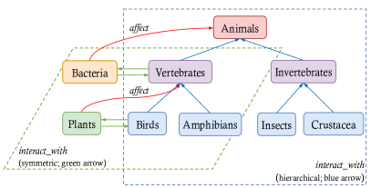
Figure 1: interacts_with is symmetric (green arrows) and hierarchical (blue arrows) in different context. Each affects (red arrow) can be composed from a green-arrow relation followed by a blue-arrow one.

Current KGE methods mainly focus on exploiting geometric transformations and embedding spaces to model relational patterns such as (anti)symmetry, inversion, and composition. TransE Bordes et al. (2013) represents each relation as a translation from a head entity to a tail entity. With translations alone, TransE cannot model many relation types such as symmetric ones. In contrast, RotatE Sun et al. (2019) represents each relation as a rotation in complex space. It proves that it can model (anti)symmetry, inversion, and composition patterns. QuatE Zhang et al. (2019) extends RotatE’s complex number representation to a hypercomplex number representation.

A drawback of rotation-based KGE models is that their representations are entrenched in (Euclidean) circular rotation, and hence they are unable to model hierarchical and tree-like structures (e.g. hypernym and part_of). Such hierarchical relations are common and even pervasive in some KGs. Since, in circular rotation, all rotating points are constrained to be at the same distance from the center of a circle, it is hard to model relations whose semantics require that entities move at different distances from the nexus.

To overcome this shortcoming, recent models project KGs into hyperbolic space Balazevic et al. (2019); Chami et al. (2020). The hyperbolic models inevitably lose the basic properties of Euclidean-space transformations, and thus cannot avail themselves of these useful operations. Moreover, it is difficult to seamlessly integrate the hyperbolic models with extant non-hyperbolic models to create more powerful hybrids because the models’ different geometric representations do not cohere.

What we want is the best of best worlds, i.e., a model capable of effecting both circular rotations and hyperbolic transformations, in a coherent geometric representation. This allows the model to choose the best representation for each relation, e.g., circular rotations for symmetric/inversion relations and hyperbolic rotations for hierarchical patterns. In addition, for relations that exhibit both circular and hyperbolic characteristics (e.g., the interact_with relation in Figure 1), the model would rely on the data to choose the sweet spot balancing both transformations. For relations that are best captured by the composition of circular and hyperbolic rotations (e.g., affects in Figure 1), the model would learn the best composition of both representations jointly. Lastly, by subsuming circular rotations, the model would inherit the representational prowess of circular-rotation models.

In this paper, we propose precisely such a model named BiQUE. BiQUE employs a powerful algebraic system called biquaternions Ward (1997) to represent KGs. Most common number systems used by current KGE methods (including real numbers, complex numbers, and real quaternions) are subsumed and systematically unified by biquaternions. Further, the Hamilton product of biquaternions, at the core of BiQUE, imbues it with a strong geometric interpretation that combines both circular rotations and hyperbolic rotations. In sum, our contributions are as follows.

• To our knowledge, we are the first to use biquaternionic algebra for KGEs. Algorithmically, we contribute by designing a flexible score function that leverages multiple geometric transformations (scaling, translation, circular rotation, and hyperbolic rotation).

• Theoretically, we contribute by rigorously proving that BiQUE’s biquaternionic transformation is equivalent to the composition of a circular rotation and a hyperbolic rotation.

• Empirically, we contribute by validating and analyzing BiQUE’s effectiveness on five KG benchmarks that span a wide gamut of sizes.

2 Related Work

We briefly survey KGE methods that are most relevant to our approach.

Euclidean models.

These models represent entities and relations by real vectors, and can be categorized into translation-based models Bordes et al. (2013); Wang et al. (2014); Lin et al. (2015); Ji et al. (2016), semantic-matching models Nickel et al. (2011); Yang et al. (2015), and neural models Dettmers et al. (2018); Vashishth et al. (2020a). Euclidean models typically cannot represent all relation types in a KG, e.g., TransE cannot model symmetric patterns, and DistMult cannot model antisymmetric/inversion patterns Sun et al. (2019). Euclidean models typically need large embedding dimensions for good empirical performance.

Complex-valued models.

ComplEx Trouillon et al. (2017) uses complex-valued tensor factorization and complex conjugation to model antisymmetric relations. RotatE Sun et al. (2019) models each relation as a 2D circular rotation in a complex vector space. It can model several relation types, but falls short when modeling hierarchical patterns. QuatE Zhang et al. (2019) extends RotatE’s complex representation to a hypercomplex one via quaternion embeddings, and represents rotations in a four-dimensional real-number space. However, it shares the weakness of circular-rotation methods in being deficient when modeling hierarchical semantics. DualE Cao et al. (2021) incorporates dual numbers into quaternions, and thereby unifies circular rotation with translation. This geometric combination of DualE differs from that of our BiQUE model (Section 4), which unifies circular rotation with hyperbolic rotation. Another difference is that BiQUE models translations via a different mechanism in the form of a relation-specific biquaternion.

Hyperbolic models.

Recent models have used hyperbolic space because of its amenability to representing hierarchical structures. MurP Balazevic et al. (2019) and ATTH Chami et al. (2020) both adopt the Poincaré-ball model to represent entities and relations. MurP utilizes Möbius multiplication and addition with relation-specific parameters to transform entities. ATTH integrates hyperbolic rotations and reflections via an attention mechanism, and learns hyperbolic curvatures automatically. Both MurP and ATTH have rigid hyperbolic geometric assumptions, and they remain challenging to optimize directly in hyperbolic space.

In contrast to existing systems, our model BiQUE overcomes their weaknesses by integrating the strengths of their respective geometric representations into one coherent representation using biquaternions. By subsuming the complex-valued rotation-based models (e.g., complEx and QuatE), it retains their strengths in capturing (anti)symmetric, inversion, and composition patterns. By incorporating a hyperbolic representation, it is also able to model hierarchical semantics.

3 Background

Biquaternions, endowed with rich algebraic properties, have been widely used in quantum mechanics, general relativity, and signal processing Pei et al. (2004); Gong et al. (2011), but have yet to make inroads into knowledge graph embeddings. A biquaternion is defined on a four-dimensional vector space over the field $\mathbb{C}$ of complex numbers. We denote a complex number $c\in\mathbb{C}$ as $c=c_{r}+c_{i}\mathbf{I}$ where $c_{r},c_{i}\in\mathbb{R}$ are real numbers, and $\mathbf{I}$ is the usual imaginary unit ($\mathbf{I}^{2}=-1$).

Definition 1.

The basic algebraic forms of a biquaternion $q$ are

$$\;\;\;\;\;\;\;\;\;\;\;\;\;\;\;\;\;\;\;\;w+x\mathbf{i}+y\mathbf{j}+z\mathbf{k}$$ (1)

$$\!=\!(w_{r}\!+\!w_{i}\mathbf{I})\!+\!(x_{r}\!+\!x_{i}\mathbf{I})\mathbf{i}\!+\!(y_{r}\!+\!y_{i}\mathbf{I})\mathbf{j}\!+\!(z_{r}\!+\!z_{i}\mathbf{I})\mathbf{k}$$

$$\!=\!q_{r}\!+\!q_{i}\mathbf{I}$$ (2)

where $w,x,y,z\!\in\!\mathbb{C}$ are $q$’s coefficients, $w_{r},x_{r},y_{r},z_{r},w_{i},x_{i},y_{i},z_{i}\!\in\!\mathbb{R}$, $q_{r}\!=\!w_{r}\!+\!x_{r}\mathbf{i}\!+\!y_{r}\mathbf{j}\!+\!z_{r}\mathbf{k}$, $q_{i}\!=\!w_{i}\!+\!x_{i}\mathbf{i}\!+\!y_{i}\mathbf{j}\!+\!z_{i}\mathbf{k}$, and $\mathbf{i},\mathbf{j},\mathbf{k}$ are imaginary units that have the following (non)commutative multiplication properties:

(3)

We denote the scalar and vector parts of $q$ respectively as $s(q)\!=\!w$ and $v(q)\!=\!x\mathbf{i}\!+\!y\mathbf{j}\!+\!z\mathbf{k}$. A pure biquaternion $q$ is one with $s(q)\!=\!0$. A quaternion Hamilton (1844) is a restricted biquaternion, in which $w,x,y,z\!\in\!\mathbb{R}$ (e.g., $q_{r}$ and $q_{i}$ in Equation 2 are quaternions). Complex numbers and real numbers are both special cases of biquaternions.

The biquaternion $q\!=\!w\!+\!x\mathbf{i}\!+\!y\mathbf{j}\!+\!z\mathbf{k}$ has several equivalent representations Ward (1997); Jafari (2016): (a) as the vector $\mathcal{V}(q)=[w,x,y,z]^{T}$; (b) as $||q||(\cos\theta\!+\!u\sin\theta)$ (where $\theta\!=\!\cos^{-1}(w/||q||)$, $\theta\!\in\!\mathbb{C}$, $u\!=\!v(q)/||v(q)||$, and $||q||\!=\!\sqrt{w^{2}\!+\!x^{2}\!+\!y^{2}\!+\!z^{2}}$); and (c) as the matrix

$$\mathcal{M}(q)=\left[\begin{array}[]{rrrr}w\!&\!-x\!&\!-y\!&\!-z\\ x\!&\!w\!&\!z\!&\!-y\\ y\!&\!-z\!&\!w\!&\!x\\ z\!&\!y\!&\!-x\!&\!w\\ \end{array}\right].$$ (4)

Next we present basic operations on a biquaternion $q\!=\!w\!+\!x\mathbf{i}\!+\!y\mathbf{j}\!+\!z\mathbf{k}$. The conjugate of $q$ is denoted as $\bar{q}=\!w\!-\!x\mathbf{i}\!-\!y\mathbf{j}\!-\!z\mathbf{k}$. The complex conjugate of $q$ is denoted as $q^{*}=\!w^{*}\!+\!x^{*}\mathbf{i}\!+\!y^{*}\mathbf{j}\!+\!z^{*}\mathbf{k}$ ($c^{*}\!=\!c_{r}\!-\!c_{i}\mathbf{I}$ is the standard complex conjugate of a complex number $c\!=\!c_{r}\!+\!c_{i}\mathbf{I}$). Two biquaternions $q_{1}\!=\!w_{1}\!+\!x_{1}\mathbf{i}\!+\!y_{1}\mathbf{j}\!+\!z_{1}\mathbf{k}$ and $q_{2}\!=\!w_{2}\!+\!x_{2}\mathbf{i}\!+\!y_{2}\mathbf{j}\!+\!z_{2}\mathbf{k}$ are added and subtracted (in the obvious manner) as $q_{1}\!\pm\!q_{2}\!=\!(w_{1}\!\pm\!w_{2})\!+\!(x_{1}\!\pm\!x_{2})\mathbf{i}\!+\!(y_{1}\!\pm\!y_{2})\mathbf{j}\!+\!(z_{1}\!\pm\!z_{2})\mathbf{k}$. The multiplication $q_{1}q_{2}$ between $q_{1}$ and $q_{2}$ can be obtained via standard algebraic distributivity (while obeying the properties in Equations 3, and following the normal multiplication rule of complex numbers for the products between coefficients) as

$$q_{1}q_{2}= w_{1}w_{2}\!-\!x_{1}x_{2}\!-\!y_{1}y_{2}\!-\!z_{1}z_{2}$$

$$+(w_{1}x_{2}\!+\!x_{1}w_{2}\!+\!y_{1}z_{2}\!-\!z_{1}y_{2})\mathbf{i}$$

$$+(w_{1}y_{2}\!-\!x_{1}z_{2}\!+\!y_{1}w_{2}\!+\!z_{1}x_{2})\mathbf{j}$$

$$+(w_{1}z_{2}\!+\!x_{1}y_{2}\!-\!y_{1}x_{2}\!+\!z_{1}w_{2})\mathbf{k}.$$ (5)

Equation 3 is termed the Hamilton product between $q_{1}$ amd $q_{2}$. Alternatively, the multiplication can be equivalently represented as a matrix-vector product

$$\mathcal{V}(q_{1}q_{2}) =\mathcal{M}(q_{2})\,\mathcal{V}(q_{1}),$$ (6)

or as a matrix-matrix product

$$\mathcal{M}(q_{1}q_{2})=\mathcal{M}(q_{2})\,\mathcal{M}(q_{1}).$$ (7)

Equations 6 and 7 can be easily verified by substituting in Equations 4 and 3, and using normal matrix multiplication. The set of biquaternions and the set of quaternions are both closed under multiplication, and multiplication is associative but not commutative. Also note that $\overline{q_{1}q_{2}}=\overline{q_{2}}\;\overline{q_{1}}$.

By using Equation 4, we can easily verify that $\mathcal{M}(\bar{q})=\mathcal{M}(q)^{T}$ and $\mathcal{M}(q^{*})=\mathcal{M}(q)^{*}$ (where $\mathcal{M}(\cdot)^{*}$ refers to the complex conjugation of each element in the matrix).

The norm of $q$ is given by $||q||\!=\!\sqrt{q\bar{q}}\!=\!\sqrt{\bar{q}q}\!=\!\sqrt{w^{2}\!+\!x^{2}\!+\!y^{2}\!+\!z^{2}}$ (NB: $||q||\!=\!||\bar{q}||$). A unit biquaternion is one with unit norm, i.e., $||q||=1$.

4 BiQUE: Biquaternionic Embeddings

4.1 Unification of Circular and Hyperbolic Rotations

We prove that a biquaternion unifies both circular and hyperbolic rotations in $\mathbb{C}^{4}$ space within a single representation in Theorem 4.1 (the proof is in Appendix A).

Theorem 4.1.

Let $\mathcal{M}(q)$ be the matrix representation of a unit biquaternion $q\!=\!q_{r}\!+\!q_{i}\mathbf{I}$, where $q_{r}\!=\!w_{r}\!+\!x_{r}\mathbf{i}\!+\!y_{r}\mathbf{j}\!+\!z_{r}\mathbf{k}$, and $q_{i}\!=\!w_{i}\!+\!x_{i}\mathbf{i}\!+\!y_{i}\mathbf{j}\!+\!z_{i}\mathbf{k}$. $\mathcal{M}(q)$ can be factorized as $\mathcal{M}(q)\!=\!\mathcal{M}(h)\,\mathcal{M}(u)$ where $\mathcal{M}(h)\!=\!$

$$\!\left[\!\!\begin{array}[]{rrrr}\cosh\phi\!&\!-a\mathbf{I}\sinh\phi\!&\!-b\mathbf{I}\sinh\phi\!&\!-c\mathbf{I}\sinh\phi\\ a\mathbf{I}\sinh\phi\!&\!\cosh\phi\!&\!c\mathbf{I}\sinh\phi\!&\!-b\mathbf{I}\sinh\phi\\ b\mathbf{I}\sinh\phi\!&\!-c\mathbf{I}\sinh\phi\!&\!\cosh\phi\!&\!a\mathbf{I}\sinh\phi\\ c\mathbf{I}\sinh\phi\!&\!b\mathbf{I}\sinh\phi\!&\!-a\mathbf{I}\sinh\phi\!&\!\cosh\phi\end{array}\!\!\right]\!\!,$$

$$\mathcal{M}(u)\!=\!\!\!\left[\!\!\begin{array}[]{rrrr}\cos\theta\!&\!-\frac{x_{r}\sin\theta}{||v(q_{r})||}\!&\!-\frac{y_{r}\sin\theta}{||v(q_{r})||}\!&\!-\frac{z_{r}\sin\theta}{||v(q_{r})||}\\ \frac{x_{r}\sin\theta}{||v(q_{r})||}\!&\!\cos\theta\!&\!\frac{z_{r}\sin\theta}{||v(q_{r})||}\!&\!-\frac{y_{r}\sin\theta}{||v(q_{r})||}\\ \frac{y_{r}\sin\theta}{||v(q_{r})||}\!&\!-\frac{z_{r}\sin\theta}{||v(q_{r})||}\!&\!\cos\theta\!&\!\frac{x_{r}\sin\theta}{||v(q_{r})||}\\ \frac{z_{r}\sin\theta}{||v(q_{r})||}\!&\!\frac{y_{r}\sin\theta}{||v(q_{r})||}\!&\!-\frac{x_{r}\sin\theta}{||v(q_{r})||}\!&\!\cos\theta\end{array}\!\!\right]\!\!,$$

$\theta\!=\!\cos^{-1}\frac{w_{r}}{||q_{r}||}$, $\phi\!=\!\cosh^{-1}||q_{r}||$, $\frac{\overline{q_{r}}q_{i}}{||q_{r}||||q_{i}||}\!=\!a\mathbf{i}\!+\!b\mathbf{j}\!+\!c\mathbf{k}$, and $\theta,\phi,a,b,c\in\mathbb{R}$. Alternatively, $\mathcal{M}(q)$ can be factorized as $\mathcal{M}(q)\!=\!\mathcal{M}(u)\,\mathcal{M}(h^{\prime})$, where $\frac{q_{i}\overline{q_{r}}}{||q_{i}||||q_{r}||}\!=\!a^{\prime}\mathbf{i}\!+\!b^{\prime}\mathbf{j}\!+\!c^{\prime}\mathbf{k}$, and $\mathcal{M}(h^{\prime})\!=\!$

In addition, the determinants of $\mathcal{M}(h)$, $\mathcal{M}(h^{\prime})$ and $\mathcal{M}(u)$ are 1, and $\mathcal{M}(h)$, $\mathcal{M}(h^{\prime})$ and $\mathcal{M}(u)$ are orthogonal.

From Theorem 4.1, we know that the matrix $\mathcal{M}(q)$, representing a unit biquaternion $q$, can be expressed as the composition of two matrices $\mathcal{M}(h)$ and $\mathcal{M}(u)$ (or $\mathcal{M}(u)$ and $\mathcal{M}(h^{\prime})$). Further, since all elements in $\mathcal{M}(h)$, $\mathcal{M}(h^{\prime})$, and $\mathcal{M}(u)$ are derived from $q$, we can construct $\mathcal{M}(h)$, $\mathcal{M}(h^{\prime})$, and $\mathcal{M}(u)$ given $q$.

An orthogonal matrix with determinant 1 represents a rotation in the space in which it operates Artin (1957). Since we know both $\mathcal{M}(h)$ and $\mathcal{M}(u)$ are orthogonal and have determinants 1 from Theorem 4.1, they each represent a rotation in $\mathbb{C}^{4}$ space. From the form of the matrices, we can see that $\mathcal{M}(u)$ represents a circular rotation, while $\mathcal{M}(h)$ represents a hyperbolic rotation. To see the hyperbolic-rotation nature of $\mathcal{M}(h)$ more clearly, we can use the identities $\cosh\phi\!=\!\cos\mathbf{I}\phi$ and $\mathbf{I}\sinh\phi\!=\!\sin\mathbf{I}\phi$ to represent $\mathcal{M}(h)$ as

$$\left[\begin{array}[]{rrrr}\cos\mathbf{I}\phi\!&\!-a\sin\mathbf{I}\phi\!&\!-b\sin\mathbf{I}\phi\!&\!-c\sin\mathbf{I}\phi\\ a\sin\mathbf{I}\phi\!&\!\cos\mathbf{I}\phi\!&\!c\sin\mathbf{I}\phi\!&\!-b\sin\mathbf{I}\phi\\ b\sin\mathbf{I}\phi\!&\!-c\sin\mathbf{I}\phi\!&\!\cos\mathbf{I}\phi\!&\!a\sin\mathbf{I}\phi\\ c\sin\mathbf{I}\phi\!&\!b\sin\mathbf{I}\phi\!&\!-a\sin\mathbf{I}\phi\!&\!\cos\mathbf{I}\phi\end{array}\right].$$

Now $\mathcal{M}(h)$ takes the form of a “regular” rotation matrix (cf. $\mathcal{M}(u)$), but with a complex angle $\mathbf{I}\phi$. According to Lansey (2009), a rotation through an imaginary angle $\mathbf{I}\phi$ can be understood as a hyperbolic rotation through the real angle $\phi$. Consequently, a unit biquaternion composes these two kinds of rotations in a coherent algebraic representation. (It has been shown by Jafari (2016, Corollary 4.1) that $\mathcal{M}(q)$ is orthogonal with a determinant of 1, and thus represents an arbitrary rotation in $\mathbb{C}^{4}$. However, that paper does not tease apart the matrix to reveal the contributions of its component circular and hyperbolic rotation matrices like we have done.)

Our results extend to arbitrary (not necessarily unit) biquaternions. Any biquaternion $q$ is a scaled version of its unit biquaternion, i.e., $q=||q||(\frac{q}{||q||})$. Thus its matrix $\mathcal{M}(q)$ represents a circular rotation followed by a hyperbolic rotation (i.e., $\mathcal{M}(h)\mathcal{M}(u)$), or a hyperbolic rotation followed by a circular rotation (i.e., $\mathcal{M}(u)\mathcal{M}(h^{\prime})$). Both rotations are represented by $\frac{q}{||q||}$, followed by a scaling by $||q||$.

We analyze and visualize the $M(u)$ and $M(h)$ rotations in Appendix B.

It is worth noting that the system QuatE² Zhang et al. (2019), an experimental baseline in Section 5, uses quaternions as its representation. Because quaternions are special cases of biquaternions, QuatE² only employs the circular rotation matrix $M(u)$ (with its $M(h)$ as the identity matrix). Further, note that the power of a biquaternion does not merely comes from doubling the parameters of a quaternion. A biquaternion achieves better representational power and parameter efficiency by facilitating the interactions between its real and imaginary parameters (see the last paragraph of Section B of the Appendix, and subsection 5.5.3).

4.2 Problem Definition

A multi-relational knowledge graph $\mathcal{KG}$ is represented as a set of directed triples, i.e., $\mathcal{KG}\!=\!\{(h,r,t)\}$. Each triple $(h,r,t)$ consists of a head entity $h\!\in\!\mathcal{E}$, a relation $r\!\in\!\mathcal{R}$, and a tail entity $t\!\in\!\mathcal{E}$. The numbers of entities and relations are denoted as $|\mathcal{E}|\!=\!N_{e}$ and $|\mathcal{R}|\!=\!N_{r}$ respectively. The goal of a knowledge graph embedding model is to project entities and relations into a continuous vector space while preserving their original semantics. The knowledge graph completion (KGC) task requires a model to predict the probability of existence or correctness of unseen triples using the observed triples $\mathcal{KG}$.

4.3 The Proposed Model

In our BiQUE model, we represent the entities and relations in a $\mathcal{KG}$ as vectors of biquaternions. Let $\mathbb{Q}$ be the set of biquaternions. Each entity $e$ is a vector $Q_{e}$ of $k$ biquaternions, i.e., $Q_{e}=[q_{1},q_{2},\ldots,q_{k}]^{T}$, where $q_{1},q_{2},\ldots,q_{k}\in\mathbb{Q}$. We denote a head entity and a tail entity as $Q_{h}$ and $Q_{t}$ respectively. Each relation $r$ is modeled as two vectors $Q_{r}^{+}$ and $Q_{r}^{\times}$, each of which also contains $k$ biquaternions. An entity or relation vector $Q\in\{Q_{h},Q_{t},Q_{r}^{+},Q_{r}^{\times}\}$ can also be expressed as $Q\!=\!w\!+\!x\mathbf{i}\!+\!y\mathbf{j}\!+\!z\mathbf{k}$ where $w,x,y,z\!\in\!\mathbb{C}^{k}$ (i.e., $w,x,y,z$ are each a vector containing $k$ complex numbers, with its $i^{th}$ element corresponding to the $i^{th}$ biquaternion in $Q$). (Note the similarity between the form of $Q$ and that of a biquaternion in Equation 1.) Because a complex number can be represented by two real numbers (its real and imaginary components), $Q$ can be represented with $k\times 4\times 2=8k$ real numbers ($8k$ is its embedding size). (For expository convenience, we refer to $Q$ as a “biquaternion” or an “embedding”; their structures should be clear from their contexts.)

Currently, the loss functions of KGE models can be roughly categorized as additive and multiplicative ones depending on the relation transformation projecting a head entity to a tail entity. Allen et al. (2021) has recently shown that projections require matrix multiplication, and cannot be achieved via addition alone. Thus, it is necessary to combine both additive and multiplicative operations into a loss function to represent powerful projections.

We represent the transformation due to relation $r$ with the biquaternions $Q_{r}^{+}$ and $Q_{r}^{\times}$. The embedding $Q_{r}^{+}$ applies a relation-specific translation to a head entity’s embedding $Q_{h}$. We realize it by the element-wise addition of biquaternions (similar to what we do with real vectors for translation):

$$\begin{aligned} Q_{h,r}^{\prime}&=Q_{h}+Q_{r}^{+}\\ &=(w_{h}+w_{r}^{+})+(x_{h}+x_{r}^{+})\mathbf{i}\\ &\ \ \ \ \ \ \ +(y_{h}+y_{r}^{+})\mathbf{j}+(z_{h}+z_{r}^{+})\mathbf{k}\\ &=w^{\prime}+x^{\prime}\mathbf{i}+y^{\prime}\mathbf{j}+z^{\prime}\mathbf{k}\end{aligned}$$ (8)

Next the embedding $Q_{r}^{\times}$ applies a relation-specific multiplicative transformation to the translated head entity $Q_{h,r}^{\prime}$. The multiplicative transformation is defined via the Hamilton product of biquaternions (Equation 3) as follows.

where $\circledast$ denotes the element-wise application of the Hamilton product between $Q_{h,r}^{\prime}$ and $Q_{r}^{\times}$, and $\otimes$ denotes the element-wise multiplication between vectors of complex numbers. As shown in subsection 4.1, each biquaternion in $Q_{r}^{\times}$ represents a composition of circular rotation, hyperbolic rotation, and scaling. In the above Hamilton product, we bring this powerful composition to bear on the projection of the translated head entity. The Hamilton product of biquaternions in Equation 9 has an added benefit of increasing the potential interaction between entities and relations through the multiplications between different components of the entities and relations (observe that each element in $\{w^{\prime},x^{\prime},y^{\prime},z^{\prime}\}$ is multiplied with each element in $\{w_{r}^{\times},x_{r}^{\times},y_{r}^{\times},z_{r}^{\times}\}$.)

Overall, our model unifies multiple expressive geometric transformations (translation, scaling, circular rotation, and hyperbolic rotation) into one coherent representation system.

4.4 Score Function and Training Loss

We measure the plausibility score of a given triple $(h,r,t)$ by computing the vector similarity between the transformed head entity $\widehat{Q_{h,r}}\!=\!\widehat{w}\!+\!\widehat{x}\mathbf{i}\!+\!\widehat{y}\mathbf{j}\!+\!\widehat{z}\mathbf{k}$ (from Equation 9), and a candidate tail entity $Q_{t}\!=\!w_{t}\!+\!x_{t}\mathbf{i}\!+\!y_{t}\mathbf{j}\!+\!z_{t}\mathbf{k}$ as

$$\begin{aligned} &\ \ \ \ \ f(h,r,t)=\widehat{Q_{h,r}}\cdot Q_{t}\\ &=\langle\widehat{w},w_{t}\rangle+\langle\widehat{x},x_{t}\rangle+\langle\widehat{y},y_{t}\rangle+\langle\widehat{z},z_{t}\rangle,\end{aligned}$$ (10)

where $\langle\cdot,\cdot\rangle$ denotes the standard dot-product between vectors.

We regard the task of knowledge graph completion as a multi-class classification problem and employ the cross-entropy loss to train our model.

$$\mathcal{L}=\sum_{(h,r,t)\in\mathcal{KG}} \sum_{t^{\prime}\in\mathcal{E}}\log\big{(}1\!+\!\exp\big{(}y_{t}f(h,r,t^{\prime})\big{)}\big{)}\!+\!\Omega$$

$$y_{t} =\left\{\begin{array}[]{rl}-1,&t^{\prime}=t\\ 1,&\text{otherwise}.\end{array}\right.$$ (13)

To combat overfitting, we follow previous work Zhang et al. (2019), and append a N3 regularization norm Lacroix et al. (2018) to our loss function, thus obtaining

where $\lambda,\lambda_{1},\lambda_{2}$ are the global, entity and relation regularization hyperparameters respectively. $\|\cdot\|_{3}$ denotes $L_{3}$ norm of vectors.

5 Experiments

To validate BiQUE’s effectiveness, we conduct extensive experiments on the knowledge graph completion (KGC) task. We use three standard knowledge graph datasets, viz., WN18RR, FB15K-237, and YAGO3-10. In addition, to demonstrate BiQUE’s scalability, we run it on two huge commonsense knowledge graph datasets, viz., Concept100k and ATOMIC. Our codes and datasets are publicly available at https://github.com/guojiapub/BiQUE.

5.1 Datasets

The WN18RR Dettmers et al. (2018) and FB15K-237 Toutanova and Chen (2015) datasets are respectively subsets of WN18 and FB15K (both from Bordes et al. (2013)). (Both WN18 and FB15K have test leakage problems, which allow their test triples to be easily inferred. Thus, KGE models typically perform well on those two datasets, and they do not help to differentiate between models. Because of this, we do not use them in our experiments.) To make the KGC task more challenging, FB15K-237 and WN18RR remove the inverse relations from the original validation and test sets of WN18 and FB15K. The CN-100K Li et al. (2016) and ATOMIC Sap et al. (2019) datasets are two large knowledge graph benchmarks recently adopted for evaluating commonsense reasoning. ATOMIC mainly describes the reactions, effects, and intents of human behaviors, and represents each entity as a phrase with an average length of 4.4 words. CN-100K contains general commonsense knowledge about the world. For CN-100K and ATOMIC, we use the data splits of previous work Malaviya et al. (2020). Table 1 provides details on the datasets. (Note that the datasets span a wide range of sizes.)

Both WN18RR and YAGO3-10 contain many relations with hierarchical semantics, e.g., hypernym and part_of Chami et al. (2020). On the other hand, most of FB15K-237’s edges are antisymmetric, and it does not have much hierarchical structure Balazevic et al. (2019). The varying level of hierarchical structure in the datasets helps to highlight BiQUE’s adaptability to datasets with different relation types. ATOMIC mainly contains cause-effect relations that are not hierarchical. CN100k contains several hierarchical relations (e.g., IsA and AtLocation). Aside from their large sizes, these two datasets have the challenging feature of being extremely sparse.

Dataset	#Entities	#Relations	#Train	#Valid	#Test
FB15K-237	14,541	237	272,115	17,535	20,466
WN18RR	40,943	11	86,835	3,034	3,134
YAGO3-10	123,188	37	1,079,040	5,000	5,000
CN-100K	78334	34	100,000	1,200	1,200
ATOMIC	304,388	9	610,536	87,700	87,701

Table 1: Knowledge Graph Benchmarks.

5.2 Baselines

We compare our model to strong baselines that operate in different geometric spaces. For Euclidean space, we use TransE Bordes et al. (2013), DistMult Yang et al. (2015), ConvE Dettmers et al. (2018), InteractE Vashishth et al. (2020a), and CompGCN Vashishth et al. (2020b). For complex-valued space, we use ComplEx Trouillon et al. (2017), RotatE Sun et al. (2019), QuatE² Zhang et al. (2019) (the version with N3 regularization and reciprocal learning) and DualE¹(without type constraints) Cao et al. (2021). For hyperbolic space, we use MurP Balazevic et al. (2019) and ATTH Chami et al. (2020). For the commonsense datasets, we also include ConvTransE Shang et al. (2019).

5.3 Evaluation Protocol

We use standard evaluation metrics for the knowledge graph completion (KGC) task, viz., mean reciprocal rank (MRR) and Hits$@k$ with cut-off values $k\in\{1,3,10\}$. For both MRR and Hits$@k$, the larger the metric, the better the performance of a model. We adopt the BOTTOM setting Sun et al. (2020) when ranking candidate triples and we consistently apply it to our BiQUE model, i.e., the correct triple is always inserted at the end of a list of triples with the same plausibility scores. This is the strictest evaluation protocol for KGC tasks, and provides the best reflection of a model’s performance. Finally, we report filtered results like previous work Bordes et al. (2013) for fair comparisons. (Implementation details are in the appendix.)

	WN18RR				FB15K-237				YAGO3-10
Models	MRR	H@1	H@3	H@10	MRR	H@1	H@3	H@10	MRR	H@1	H@3	H@10
TransE	0.226	-	-	0.501	0.294	-	-	0.465	-	-	-	-
DistMult	0.430	0.390	0.440	0.490	0.241	0.155	0.263	0.419	0.340	0.240	0.380	0.540
ConvE	0.430	0.400	0.440	0.520	0.325	0.237	0.356	0.501	0.440	0.350	0.490	0.620
InteractE	0.463	0.430	-	0.528	0.354	0.263	-	0.535	0.541	0.462	-	0.687
CompGCN	0.479	0.443	0.494	0.546	0.355	0.264	0.390	0.535	-	-	-	-
ComplEx-N3	0.480	0.435	0.495	0.572	0.357	0.264	0.392	0.547	0.569	0.498	0.609	0.701
RotatE	0.476	0.428	0.492	0.571	0.338	0.241	0.375	0.533	0.495	0.402	0.550	0.670
QuatE2	0.482	0.436	0.499	0.572	0.366	0.271	0.401	0.556	0.568	0.493	0.611	0.706
DualE1	0.482	0.440	0.500	0.561	0.330	0.237	0.363	0.518	-	-	-	-
MurP	0.481	0.440	0.495	0.566	0.335	0.243	0.367	0.518	0.354	0.249	0.400	0.567
ATTH	0.486	0.443	0.499	0.573	0.348	0.252	0.384	0.540	0.568	0.493	0.612	0.702
BiQUE	0.504	0.459	0.519	0.588	0.365	0.270	0.401	0.555	0.581	0.509	0.624	0.713

Table 2: Best results are bolded, and second best results are underlined. Results for DistMult, ConvE, ComplEx-N3, RotatE, MurP, and ATTH are from Chami et al. (2020). Results for TransE and QuatE² are from Zhang et al. (2019). Results for InteractE, CompGCN and DualE¹ are from their original papers. YAGO3 results for QuatE² are obtained using our implementation (QuatE² can be viewed as a special case of BiQUE as discussed in Section 4.1).

	CN-100K				ATOMIC
Models	MRR	H@1	H@3	H@10	MRR	H@1	H@3	H@10
DistMult	0.090	0.045	0.098	0.174	0.124	0.092	0.152	0.183
ComplEx	0.114	0.074	0.125	0.190	0.142	0.133	0.141	0.160
ConvE	0.209	0.140	0.229	0.340	0.101	0.082	0.103	0.134
RotatE	0.247	-	0.282	0.454	0.112	-	0.115	0.156
ConvTransE	0.187	0.079	0.239	0.390	0.129	0.129	0.130	0.130
QuatE2	0.313	0.217	0.356	0.504	0.187	0.167	0.191	0.225
BiQUE	0.320	0.216	0.359	0.553	0.191	0.171	0.196	0.230

Table 3: Best results are bolded, and second best results are underlined. Results for DistMult, ComplEx, ConvE, and ConvTransE are from Malaviya et al. (2020). Results for RotatE are from Wang et al. (2020). Results for QuatE² are obtained using our implementation (QuatE² is a special case of BiQUE as discussed in Section 4.1).

5.4 Results

Table 2 shows the experimental results. Following standard practice adopted by our comparison systems, we show the best results for BiQUE. (We pick the best result over 10 runs with different random initializations. The appendix contains the average scores over the runs, and the standard deviations.)

From Table 2, we see that BiQUE is the best performer on four of the five datasets, and is a close second on the remaining dataset. On the two hierarchical datasets WN18RR and YAGO3-10, BiQUE achieves new state-of-the-art results on all metrics, and surpasses the second best models by a clear margin. WN18RR contains a large proportion of symmetric relations (which are amenable to being modeled with circular rotations) and hierarchical relations (which are amenable to being modeled with hyperbolic rotations). BiQUE’s good performance on this dataset provides evidence that BiQUE’s composition of circular and hyperbolic rotations is useful in modeling these disparate relation types simultaneously. BiQUE also consistently outperforms the hyperbolic models MurP and AttH on all metrics.

On FB15K-237, BiQUE is second best; however, BiQUE’s scores are only marginally lower than those of the best system QuatE². As observed by Balazevic et al. (2019), the vast majority of relations in FB15K-237 do not form hierarchies. Consequently, BiQUE’s hyperbolic transformation does not play a principal role on FB15K-237, and BiQUE falls back on only using its circular rotation transformation. QuatE² can be viewed as a special case of BiQUE that only has circular rotations ($\mathcal{M}(u)$ in Thoerem 4.1). Since both use the same transformation, their results are (almost) indistinguishable on FB15K-237.

Table 3 shows the results on the large commonsense graphs, CN-100K and ATOMIC. We see that these datasets are a lot more challenging with many KGE models having MRRs below or hovering around 0.3. (Because of the datasets’ large sizes, many extant KGE models do not experiment on them, and we compare against the models that have been reported in the literature. Malaviya et al. (2020) describes systems that use BERT embeddings, and thus encapsulate a lot of commonsense prior knowledge; for a fair comparison, we do not use such systems as baselines.) Table 3 shows that BiQUE outperforms the previously reported state-of-the-art results on CN-100K (RotatE) and ATOMIC (ComplEx) (by 29.6% and 34.5% on MRR respectively). Further, by composing hyperbolic rotation with circular rotation, BiQUE surpasses QuatE² that only uses the latter rotation.

Relation Name	#Tripes	RotH	QuatE2	BiQUE	Lift
hypernym	1,251	0.276	0.283	0.306	8.13%
derivationally_related_form	1,074	0.968	0.969	0.970	0.10%
instance_hypernym	122	0.520	0.549	0.602	9.65%
also_see	56	0.705	0.688	0.750	6.38%
member_meronym	253	0.399	0.389	0.453	13.53%
synset_domain_topic_of	114	0.447	0.518	0.539	4.05%
has_part	172	0.346	0.337	0.392	13.29%
member_of_domain_usage	24	0.438	0.563	0.563	-
member_of_domain_region	26	0.365	0.327	0.500	36.99%
verb_group	39	0.974	0.974	0.974	-
similar_to	3	1.000	1.000	1.000	-

Table 4: Best results are bolded, and second best results are underlined. Comparison of H@10 per relation for BiQUE and baselines on WN18RR. Results for RotH are from Chami et al. (2020). QuatE²’s results are obtained by running its official code (%****␣expts.tex␣Line␣175␣****https://github.com/cheungdaven/QuatE)

5.5 Analysis

5.5.1 Performance per Relation

To provide a fine-grained analysis of BiQUE’s results, we report its performance per relation on WN18RR in Table 4. A large portion of the WN18RR dataset consists of hierarchical triples, such as hypernym and instance_hypernym, which account for more than 43% of training examples. We see that BiQUE achieves the best performance on all 11 relation types compared with current top-performing models. BiQUE not only performs well on hierarchical and tree-like relations (e.g., hypernym and instance_hypernym), but also obtains significant improvements on challenging one-to-many relations (e.g., member_of_domain_region and member_meronym). It is worth noting that BiQUE does not sacrifice its performance on other relation types for the abovementioned improvements. In fact, BiQUE also achieves the best performance for symmetric relations (e.g., derivationally_related_form and verb_group). All in all, these fine-grained results support our hypothesis that BiQUE’s integration of multiple geometric transformations allows it to make good trade-offs among various representations for different relation types, thereby allowing it to pick the best one (or combinations thereof) for optimal performance.

5.5.2 Model Variants and Ablation Study

Table 5 shows the performances of variants and ablations of BiQUE. We test the impact of BiQUE’s scaling operation by normalizing the relation rotation biquaternion $Q_{r}^{\times}$ in two ways: $Q_{r}^{\times\star}$ uses the regular normalization of real vectors, and $Q_{r}^{\times\triangleleft}$ uses the standard normalization of biquaternions. (See appendix for details.) Compared to BiQUE, both normalized variants perform worse. Thus the norm of $Q_{r}^{\times}$ plays an important role in having a scaling effect. Further, from our ablation study, we observe that without the translation operator $Q_{r}^{+}$, BiQUE performs worse on both datasets. This shows that rotations cannot fully replace translations in KGE models. Table 5 also shows that regularization is important for BiQUE to avoid overfitting.

Variants	WN18RR		FB15K-237
	MRR	H@3	MRR	H@3
BiQUE	0.504	0.519	0.365	0.401
$\big{(}(Q_{h}+Q_{r}^{+})\circledast Q_{r}^{\times\star}\big{)}\cdot Q_{t}$	0.491	0.502	0.351	0.384
$\big{(}(Q_{h}+Q_{r}^{+})\circledast Q_{r}^{\times\triangleleft}\big{)}\cdot Q_{t}$	0.486	0.500	0.350	0.385
w/o $Q_{r}^{+}$	0.490	0.505	0.362	0.398
w/o regularizer	0.457	0.467	0.344	0.378

Table 5: Variants and ablations of BiQUE on WN18RR.

5.5.3 Model Efficiency

We investigate the impact of varying embedding size on performance (H$@$1). In Figure 2, the parameters of all systems are tuned, and the results are averaged over 5 runs (with different random initializations). We see that BiQUE’s results consistently surpasses those of the strong baselines across embedding dimensions. The disparity is most apparent in the regime of small embedding sizes. This suggests that BiQUE’s representation is more effective at modeling the data (and thus do better even with smaller embeddings).

In Table 6, we use the same number of parameters for BiQUE and QuatE² (the baseline most similar to BiQUE), and show that BiQUE performs better (higher MRR and H$@$3) with fewer epochs. This again supports our hypothesis that BiQUE models the data better (with the same number of parameters) than QuatE², and thus requires fewer epochs to achieve better results.

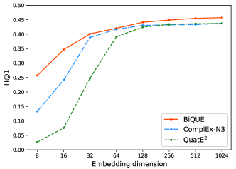
Figure 2: Effect of varying embedding size on performance.

WN18RR FB15K-237 #Params #Epoch MRR H@3 #params #Epoch MRR H@3 QuatE² 20.97M 40000 0.481 0.496 7.57M 15000 0.331 0.363 BiQUE 200 0.499 0.515 300 0.359 0.397

Table 6: Performance on WN18RR and FB15K-237 with the same parameter size.

6 Conclusion

In this paper, we propose BiQUE, a novel model that uses biquaternionic algebra for KGEs, and combines multiple geometric transformations in a coherent representation. Our experimental results and detailed empirical analysis demonstrate the effectiveness, scalability, and advantages of our model. As future work, we will extend BiQUE to work on knowledge hypergraphs.

Appendix A Proofs

We prove that a biquaternion unifies both circular and hyperbolic rotations in $\mathbb{C}^{4}$ space within a single representation in Theorem 4.1. To do so, we require Theorem A.1 that is proved by Jafari (2016), and the definitions covered in Section 3. We also prove auxiliary Lemma A.2.

Theorem A.1 (Jafari, 2016, Theorem 4.1(vi)).

If $\mathcal{M}(q)$ is the matrix representation of a biquaternion $q$, then the matrix’s determinant is given by $\det[\mathcal{M}(q)]=||q||^{4}$.

Lemma A.2.

If $q\!=\!q_{r}\!+\!q_{i}\mathbf{I}$ is a unit biquaternion (i.e., $||q||\!=\!1$) where $q_{r}\!=\!w_{r}\!+\!x_{r}\mathbf{i}\!+\!y_{r}\mathbf{j}\!+\!z_{r}\mathbf{k}$, and $q_{i}\!=\!w_{i}\!+\!x_{i}\mathbf{i}\!+\!y_{i}\mathbf{j}\!+\!z_{i}\mathbf{k}$, then $\overline{q_{r}}q_{i}$ and $q_{i}\overline{q_{r}}$ are pure quaternions (i.e., their scalar parts $s(\overline{q_{r}}q_{i})\!=\!s(q_{i}\overline{q_{r}})\!=\!0$), $||q_{r}||\!=\!\cosh\phi$ and $||q_{i}||\!=\!\sinh\phi\;$, where $\phi\in\mathbb{R}$.

Proof.

Note that both $q_{r}$ and $q_{i}$ are quaternions, and $q\!=\!(w_{r}\!+\!w_{i}\mathbf{I})\!+\!(x_{r}\!+\!x_{i}\mathbf{I})\mathbf{i}\!+\!(y_{r}\!+\!y_{i}\mathbf{I})\mathbf{j}\!+\!(z_{r}\!+\!z_{i}\mathbf{I})\mathbf{k}$.

$$||q||^{2}\!= (w_{r}\!+\!w_{i}\mathbf{I})^{2}\!+\!(x_{r}\!+\!x_{i}\mathbf{I})^{2}\!+\!(y_{r}\!+\!y_{i}\mathbf{I})^{2}$$

$$+\!(z_{r}\!+\!z_{i}\mathbf{I})^{2}$$

$$\!= (w_{r}^{2}\!-\!w_{i}^{2}+x_{r}^{2}\!-\!x_{i}^{2}+y_{r}^{2}\!-\!y_{i}^{2}+z_{r}^{2}\!-\!z_{i}^{2})$$

$$+2(w_{r}w_{i}+x_{r}x_{i}+y_{r}y_{i}+z_{r}z_{i})\mathbf{I}.$$

Since $||q||^{2}=1$ is real, we know that the above imaginary part $w_{r}w_{i}+x_{r}x_{i}+y_{r}y_{i}+z_{r}z_{i}=0$.

$$s(\overline{q_{r}}q_{i})\!= s((w_{r}\!-\!x_{r}\mathbf{i}\!-\!y_{r}\mathbf{j}\!-\!z_{r}\mathbf{k})\cdot$$

$$\;\;\;\;\;\;\;(w_{i}\!+\!x_{i}\mathbf{i}\!+\!y_{i}\mathbf{j}\!+\!z_{i}\mathbf{k}))$$

$$= \;w_{r}w_{i}+x_{r}x_{i}+y_{r}y_{i}+z_{r}z_{i}\;\;\mbox{(using Eq.~{}\ref{eqn:hamproduct})}$$

$$= \;0.$$

$$s(q_{i}\overline{q_{r}})\!= s((w_{i}\!+\!x_{i}\mathbf{i}\!+\!y_{i}\mathbf{j}\!+\!z_{i}\mathbf{k})\cdot$$

$$\;\;\;\;\;\;\;(w_{r}\!-\!x_{r}\mathbf{i}\!-\!y_{r}\mathbf{j}\!-\!z_{r}\mathbf{k}))$$

$$= \;w_{i}w_{r}+x_{i}x_{r}+y_{i}y_{r}+z_{i}z_{r}\;\;\mbox{(using Eq.~{}\ref{eqn:hamproduct})}$$

$$= \;0.$$

Thus $\overline{q_{r}}q_{i}$ and $q_{i}\overline{q_{r}}$ are both pure quaternions (recall that the set of quaternions is closed under multiplication).

$$||q||^{2}\!=\!\bar{q}q\!=\!\overline{(q_{r}\!+\!q_{i}\mathbf{I})}(q_{r}\!+\!q_{i}\mathbf{I})\!=\!(\overline{q_{r}}\!+\!\overline{q_{i}}\mathbf{I})(q_{r}\!+\!q_{i}\mathbf{I})$$

$$\!=\!\overline{q_{r}}q_{r}+\overline{q_{i}}q_{i}\mathbf{I}^{2}+(\overline{q_{r}}q_{i}+\overline{q_{i}}q_{r})\mathbf{I}$$

$$\!=\!||q_{r}||^{2}-||q_{i}||^{2}+(\overline{q_{r}}q_{i}+\overline{q_{i}}q_{r})\mathbf{I}.$$

Since $||q||^{2}\!=\!1$ is real, $\overline{q_{r}}q_{i}\!+\!\overline{q_{i}}q_{r}\!=\!0$ and $||q_{r}||^{2}\!-\!||q_{i}||^{2}\!=\!1$. The latter is the equation of a hyperbola. Since $||q_{r}||$ is real, there must exist $\phi\in\mathbb{R}$ such that $||q_{r}||=\cosh\phi$ and $||q_{i}||=\sinh\phi$ (which gives the identity $\cosh^{2}\phi-\sinh^{2}\phi=1$). ∎

Theorem 4.1.

Let $\mathcal{M}(q)$ be the matrix representation of a unit biquaternion $q\!=\!q_{r}\!+\!q_{i}\mathbf{I}$, where $q_{r}\!=\!w_{r}\!+\!x_{r}\mathbf{i}\!+\!y_{r}\mathbf{j}\!+\!z_{r}\mathbf{k}$, and $q_{i}\!=\!w_{i}\!+\!x_{i}\mathbf{i}\!+\!y_{i}\mathbf{j}\!+\!z_{i}\mathbf{k}$. $\mathcal{M}(q)$ can be factorized as $\mathcal{M}(q)\!=\!\mathcal{M}(h)\,\mathcal{M}(u)$ where $\mathcal{M}(h)\!=\!$

$$\!\left[\!\!\begin{array}[]{rrrr}\cosh\phi\!&\!-a\mathbf{I}\sinh\phi\!&\!-b\mathbf{I}\sinh\phi\!&\!-c\mathbf{I}\sinh\phi\\ a\mathbf{I}\sinh\phi\!&\!\cosh\phi\!&\!c\mathbf{I}\sinh\phi\!&\!-b\mathbf{I}\sinh\phi\\ b\mathbf{I}\sinh\phi\!&\!-c\mathbf{I}\sinh\phi\!&\!\cosh\phi\!&\!a\mathbf{I}\sinh\phi\\ c\mathbf{I}\sinh\phi\!&\!b\mathbf{I}\sinh\phi\!&\!-a\mathbf{I}\sinh\phi\!&\!\cosh\phi\end{array}\!\!\right]\!\!,$$

$$\mathcal{M}(u)\!=\!\!\!\left[\!\!\begin{array}[]{rrrr}\cos\theta\!&\!-\frac{x_{r}\sin\theta}{||v(q_{r})||}\!&\!-\frac{y_{r}\sin\theta}{||v(q_{r})||}\!&\!-\frac{z_{r}\sin\theta}{||v(q_{r})||}\\ \frac{x_{r}\sin\theta}{||v(q_{r})||}\!&\!\cos\theta\!&\!\frac{z_{r}\sin\theta}{||v(q_{r})||}\!&\!-\frac{y_{r}\sin\theta}{||v(q_{r})||}\\ \frac{y_{r}\sin\theta}{||v(q_{r})||}\!&\!-\frac{z_{r}\sin\theta}{||v(q_{r})||}\!&\!\cos\theta\!&\!\frac{x_{r}\sin\theta}{||v(q_{r})||}\\ \frac{z_{r}\sin\theta}{||v(q_{r})||}\!&\!\frac{y_{r}\sin\theta}{||v(q_{r})||}\!&\!-\frac{x_{r}\sin\theta}{||v(q_{r})||}\!&\!\cos\theta\end{array}\!\!\right]\!\!,$$

$\theta\!=\!\cos^{-1}\frac{w_{r}}{||q_{r}||}$, $\phi\!=\!\cosh^{-1}||q_{r}||$, $\frac{\overline{q_{r}}q_{i}}{||q_{r}||||q_{i}||}\!=\!a\mathbf{i}\!+\!b\mathbf{j}\!+\!c\mathbf{k}$, and $\theta,\phi,a,b,c\in\mathbb{R}$. Alternatively, $\mathcal{M}(q)$ can be factorized as $\mathcal{M}(q)\!=\!\mathcal{M}(u)\,\mathcal{M}(h^{\prime})$, where $\frac{q_{i}\overline{q_{r}}}{||q_{i}||||q_{r}||}\!=\!a^{\prime}\mathbf{i}\!+\!b^{\prime}\mathbf{j}\!+\!c^{\prime}\mathbf{k}$, and $\mathcal{M}(h^{\prime})\!=\!$

In addition, the determinants of $\mathcal{M}(h)$, $\mathcal{M}(h^{\prime})$ and $\mathcal{M}(u)$ are 1, and $\mathcal{M}(h)$, $\mathcal{M}(h^{\prime})$ and $\mathcal{M}(u)$ are orthogonal.

Proof.

We utilize the ansatzes $u=\frac{q_{r}}{||q_{r}||}$, $h=||q_{r}||+\mathbf{I}\frac{\overline{q_{r}}q_{i}}{||q_{r}||||q_{i}||}||q_{i}||$, and $h^{\prime}=||q_{r}||+$ $\mathbf{I}\frac{q_{i}\overline{q_{r}}}{||q_{i}||||q_{r}||}||q_{i}||$ Note that $u$ is a unit quaternion ($q_{r}$ normalized), and $h$ is a biquaternion in which $\frac{\overline{q_{r}}q_{i}}{||q_{r}||||q_{i}||}$ is a quaternion that is both pure (using Lemma A.2) and of unit norm (it is a product of two unit quaternions $\frac{\overline{q_{r}}}{||q_{r}||}\!=\!\frac{\overline{q_{r}}}{||\overline{q_{r}}||}$ and $\frac{q_{i}}{||q_{i}||}$). Similarly, $h^{\prime}$ is a biquaternion in which $\frac{q_{i}\overline{q_{r}}}{||q_{i}||||q_{r}||}$ is a quaternion that is both pure and of unit norm. (NB: if $\alpha$ and $\beta$ are unit quaternions, then $||\alpha\beta||^{2}=\overline{\alpha\beta}\alpha\beta=\overline{\beta}\overline{\alpha}\alpha\beta=\overline{\beta}\beta=1$.)

$$uh= \frac{q_{r}}{||q_{r}||}\left(||q_{r}||+\mathbf{I}\frac{\overline{q_{r}}q_{i}}{||q_{r}||||q_{i}||}||q_{i}||\right)$$

$$= q_{r}+\mathbf{I}\frac{q_{r}\overline{q_{r}}q_{i}}{||q_{r}||||q_{r}||}=q_{r}+\mathbf{I}\frac{||q_{r}||^{2}q_{i}}{||q_{r}||^{2}}=q$$

Similarly,

$$h^{\prime}u= \left(||q_{r}||+\mathbf{I}\frac{q_{i}\overline{q_{r}}}{||q_{i}||||q_{r}||}||q_{i}||\right)\frac{q_{r}}{||q_{r}||}$$

$$= q_{r}+\mathbf{I}\frac{q_{i}\overline{q_{r}}q_{r}}{||q_{r}||||q_{r}||}$$

$$= q_{r}+\mathbf{I}\frac{q_{i}||q_{r}||^{2}}{||q_{r}||^{2}}=q\;\;\mbox{(by associativity)}$$

Using Equation 7, we get the following factorizations: $\mathcal{M}(q)\!=\!\mathcal{M}(uh)\!=\!\mathcal{M}(h)\mathcal{M}(u)$, and $\mathcal{M}(q)\!=\!\mathcal{M}(h^{\prime}u)\!=\!\mathcal{M}(u)\mathcal{M}(h^{\prime})$.

From Section 3, we know that the quaternion $u\!=\!\frac{q_{r}}{||q_{r}||}\!=\!\frac{w_{r}}{||q_{r}||}\!+\!\frac{x_{r}}{||q_{r}||}\mathbf{i}\!+\!\frac{y_{r}}{||q_{r}||}\mathbf{j}\!+\!\frac{z_{r}}{||q_{r}||}\mathbf{k}$ can be represented equivalently as $u\!=\!||u||(\cos\theta\!+\!\frac{v(u)}{||v(u)||}\sin\theta)$ $\!=\!\cos\theta\!+\!\frac{v(q_{r})}{||v(q_{r})||}\sin\theta$ (where $\theta\!=\!\cos^{-1}\frac{w_{r}}{||q_{r}||}$; $\theta\!\in\!\mathbb{R}$ because $w_{r},||q_{r}||\!\in\!\mathbb{R}$). Expanding $v(q_{r})$, we get $u=\cos\theta\!+\!\frac{x_{r}\sin\theta}{||v(q_{r})||}\mathbf{i}\!+\!\frac{y_{r}\sin\theta}{||v(q_{r})||}\mathbf{j}\!+\!\frac{z_{r}\sin\theta}{||v(q_{r})||}\mathbf{k}$. Using the matrix representation given by Equation 4, we get the form of $\mathcal{M}(u)$ as stated in the theorem.

Since $\frac{\overline{q_{r}}q_{i}}{||q_{r}||||q_{i}||}$ is a pure unit quaternion, it can be represented as $a\mathbf{i}\!+\!b\mathbf{j}\!+\!c\mathbf{k}$ ($a,b,c\in\mathbb{R}$). Thus, $h=||q_{r}||+\mathbf{I}(a\mathbf{i}\!+\!b\mathbf{j}\!+\!c\mathbf{k})||q_{i}||$ where $\frac{\overline{q_{r}}q_{i}}{||q_{r}||||q_{i}||}=a\mathbf{i}\!+\!b\mathbf{j}\!+\!c\mathbf{k}$. From Lemma A.2, $||q_{r}||=\cosh\phi$ and $||q_{i}||=\sinh\phi$. Thus $h=\cosh\phi\!+\!(a\mathbf{I}\sinh\phi)\mathbf{i}\!+\!(b\mathbf{I}\sinh\phi)\mathbf{j}\!+\!(c\mathbf{I}\sinh\phi)\mathbf{k}$. Similarly, we can obtain $h^{\prime}=\cosh\phi+(a^{\prime}\mathbf{I}\sinh\phi)\mathbf{i}+(b^{\prime}\mathbf{I}\sinh\phi)\mathbf{j}+$ $(c^{\prime}\mathbf{I}\sinh\phi)\mathbf{k}$ and $\frac{q_{i}\overline{q_{r}}}{||q_{i}||||q_{r}||}\!=\!a^{\prime}\mathbf{i}\!+\!b^{\prime}\mathbf{j}\!+\!c^{\prime}\mathbf{k}$. Again, using the the matrix representation given by Equation 4, we get the form of $\mathcal{M}(h)$ and $\mathcal{M}(h^{\prime})$ as stated in the theorem.

Note that all elements in $\mathcal{M}(h),\mathcal{M}(h^{\prime})$, and $\mathcal{M}(u)$ are derived from $q$. Hence, for any $q$, we can construct $\mathcal{M}(h)$, $\mathcal{M}(h^{\prime})$, and $\mathcal{M}(u)$, thus proving that $\mathcal{M}(q)$ can be factorized as $\mathcal{M}(q)\!=\!\mathcal{M}(h)\mathcal{M}(u)$ and $\mathcal{M}(q)=\mathcal{M}(u)\mathcal{M}(h^{\prime})$.

Next, we show that since both $u$ and $q$ are unit biquaternions, $h$ and $h^{\prime}$ is each a unit biquaternion. $q=uh\Rightarrow\bar{q}q=\overline{uh}uh=\bar{h}\bar{u}uh=\bar{h}h=||h||^{2}$. Likewise, $q=h^{\prime}u\Rightarrow q\bar{q}=h^{\prime}u\overline{h^{\prime}u}=h^{\prime}u\bar{u}\bar{h^{\prime}}=h^{\prime}\bar{h^{\prime}}=||h^{\prime}||^{2}$. Since $q$ is a unit biquaternion, $\bar{q}q=q\bar{q}=1=$ $||h||^{2}=||h^{\prime}||^{2}$.

Using Theorem A.1, we can obtain $\det\mathcal{M}(h)\!=\!||h||^{4}\!=\!1$, $\det\mathcal{M}(h^{\prime})\!=\!||h^{\prime}||^{4}\!=\!1\!$, and $\det\mathcal{M}(u)\!=\!||u||^{4}\!=\!1$.

$\bar{h}h\!=\!1\Rightarrow\mathcal{M}(h)\mathcal{M}(\bar{h})\!=\!\mathcal{M}(h)\mathcal{M}(h)^{T}\!=\!\mathcal{M}(1)\!=\!\mathbb{I}$. Likewise, $h^{\prime}\bar{h^{\prime}}\!=\!1\Rightarrow\mathcal{M}(\bar{h^{\prime}})\mathcal{M}(h^{\prime})\!=\!$ $\mathcal{M}(h^{\prime})^{T}\mathcal{M}(h^{\prime})\!=\!\mathcal{M}(1)\!=\!\mathbb{I}$, $\bar{u}u\!=\!1\Rightarrow\mathcal{M}(u)\mathcal{M}(\bar{u})$ $\!=\!\mathcal{M}(u)\mathcal{M}(u)^{T}\!=\!\mathcal{M}(1)\!=\!\mathbb{I}$. Thus $\mathcal{M}(h),\mathcal{M}(h^{\prime})$, and $\mathcal{M}(u)$ are orthogonal. ∎

Appendix B Analysis and Visualization of BiQUE’s Circular and Hyperbolic Rotations

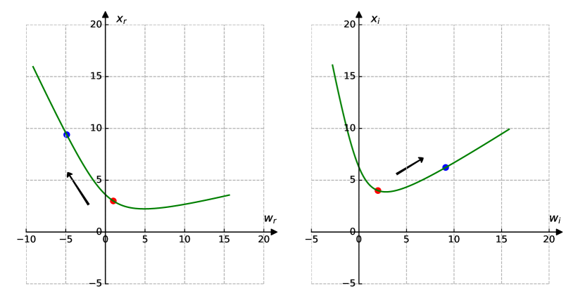
Figure 3: $M(h)$’s hyperbolic rotations in the real and imaginary parts respectively.

To analyze BiQUE’s circular and hyperbolic rotations, we restrict ourselves to two dimensions. This means a biquaternion takes the form of $q=w+x\mathbf{i}$ where $w,x\in\mathbb{C}$. The unit quaternion $q_{r}$ in Theorem 4.1 is thus $q_{r}=w_{r}+x_{r}\mathbf{i}$ where $w_{r},x_{r}\in\mathbb{R}$, and $x_{r}/||v(q_{r})||=x_{r}/||x_{r}\mathbf{i}||=1$. The circular rotation matrix is thus

$$M(u)=\begin{bmatrix}\cos\theta&-\sin\theta\\ \sin\theta&\cos\theta\end{bmatrix}$$

Now, we multiply $M(u)$ with an arbitrary biquaternion $(w_{r}+w_{i}\mathbf{I})+(x_{r}+x_{i}\mathbf{I})\mathbf{i}$ to transform it.

We can see that the real parts $w_{r},x_{r}$ and imaginary parts $w_{i},x_{i}$ are transformed independently. Hence we can accomplish the same effect by rotating two quaternions ($w_{r}+x_{r}\mathbf{i}$ and $w_{i}+x_{i}\mathbf{i}$) independently, and this does not imbue biquaternions with added representational power beyond that of quaternions, which also have the rotation $M(u)$ matrix.

Now, we examine the effect of the hyperbolic rotation matrix $M(h)$. Since $a\mathbf{i}+b\mathbf{j}+c\mathbf{k}$ is a unit quaternion (as shown in the proof of Theorem 4.1), and we restrict ourselves to two dimensions, it must be that $a=1,b=0,c=0$. The hyperbolic rotation matrix is thus

$$M(h)=\begin{bmatrix}\cosh\phi&-\mathbf{I}\sinh\phi\\ \mathbf{I}\sinh\phi&\cosh\phi\end{bmatrix}$$

We multiply $M(h)$ with an arbitrary biquaternion $(w_{r}+w_{i}\mathbf{I})+(x_{r}+x_{i}\mathbf{I})\mathbf{i}$ to transform the latter.

Observe each term in the sum now involves both the real and imaginary parts ($w_{r},x_{r},w_{i},x_{i}$) of the input biquaternion. This is unlike the case above for $M(u)$ in which the real and imaginary components are independent. Thus it is the hyperbolic rotation $M(h)$ that allows for the interaction between the real and imaginary components. To illustrate the hyperbolic rotation, we set $w_{r}=1,w_{i}=2,x_{r}=3,x_{i}=4$, and change the value of $\phi$ continually from an initial value of 0. Note that when $\phi=0$, the first term in the sum is the point $(w_{r},x_{r})$ and the second term is $(w_{i},x_{i})$. As $\phi$ changes, we can visualize the projection of that point. In Figure 3, the initial points in red are projected along the green lines. Clearly the green paths are hyperbolic. The blue point is an example of a projected point.

Appendix C Normalization of biquaternions

Given that $Q_{r}^{\times}=(w_{r}+w_{i}\mathbf{I})+(x_{r}+x_{i}\mathbf{I})\mathbf{i}+(y_{r}+y_{i}\mathbf{I})\mathbf{j}+(z_{r}+z_{i}\mathbf{I})\mathbf{k}$, let $A=(w_{r}^{2}+x_{r}^{2}+y_{r}^{2}+z_{r}^{2})$ and $B=(w_{i}^{2}+x_{i}^{2}+y_{i}^{2}+z_{i}^{2})$, we define the real vector norm $\|Q_{r}^{\times}\|_{v}$ and biquaternion norm $\|Q_{r}^{\times}\|_{b}$ as follows:

$$\begin{aligned} \|Q_{r}^{\times}\|^{2}_{v}&=A+B\\ \|Q_{r}^{\times}\|^{2}_{b}&=A-B+2(w_{r}w_{i}+x_{r}x_{i}+y_{r}y_{i}+z_{r}z_{i})\mathbf{I}\\ \end{aligned}$$

Thus, we can obtain $Q_{r}^{\times\star}$ in section 5.5.2 with the standard normalization of real vectors: $Q_{r}^{\times\star}=\frac{Q_{r}^{\times}}{\|Q_{r}^{\times}\|_{v}}$.To make $Q_{r}^{\times}$ be a unit biquaternion, we have to make sure that $A-B=1$ and $w_{r}w_{i}+x_{r}x_{i}+y_{r}y_{i}+z_{r}z_{i}=0$. We first employ the Gram-Schmidt orthogonalization technique to guarantee that the imaginary coefficient is zero and then restrict $B=1$. Alternatively, we represent $Q_{r}^{\times}$ as $Q_{r}^{\times}=q_{1}+q_{2}\mathbf{I}$, and conduct the following operations:

$$q_{1}^{\prime} =q_{1}-\frac{<q_{1},q_{2}>}{\|q_{2}\|^{2}}q_{2}$$

$$\widetilde{q_{1}} =\frac{\sqrt{2}q_{1}^{\prime}}{\|q_{1}^{\prime}\|},\ \ \widetilde{q_{2}}=\frac{q_{2}}{\|q_{2}\|}.$$

Thus, we obtain the unit biquaternion $Q_{r}^{\times\triangleleft}=\widetilde{q_{1}}+\widetilde{q_{2}}\mathbf{I}$.

Appendix D Variance of the performance

In Table 8 and 9, we provide the averages and standard deviations for all metrics on the FB15k-237, WN18RR, YAGO3-10, CN-100K and ATOMIC datasets. The results are reported based on 10 runs with different random initializations. We see that the performance of our model BiQUE is quite stable across different random initializations, and this supports the robustness of our method.

Appendix E Implementation Details

For training, we adopt reciprocal learning Lacroix et al. (2018), in which we add an inverse triple $(t,r^{-1},h)$ for each observed triple $(h,r,t)$ in the training data. For model optimization, we use Adagrad Duchi et al. (2011) as the optimizer, and employ grid search to find the best hyperparameters according to their performances on validation sets. The hyperparamters we search over includes embedding size ({128, 256, 512, 1024}), batch size ({300, 500, 1000, 2000, 5000}), learning rate ({0.1, 0.01}), and regularization parameters of Equation 14 ($\lambda$:{0, 5e-3, 1e-2, 5e-2, 7e-2, 1e-1, 1.5e-1}; $\lambda_{1}$, $\lambda_{2}$: {0.5, 1.0, 1.5, 2.0}). The parameters used in Table 2 are shown in Table 7. We implement our BiQUE model in PyTorch, and run all experiments on NVIDIA Quadro RTX 8000 GPUs.

Datasets	Epoch	Lr	Batch	$k$	$\lambda$	$\lambda_{1}$	$\lambda_{2}$
WN18RR	200	1e-1	300	128	1.5e-1	2.0	0.5
FB15K-237	300	1e-1	500	128	7e-2	2.0	0.5
YAGO3-10	200	1e-1	1000	128	5e-3	2.0	0.5
CN-100K	200	1e-1	5000	128	1e-1	2.0	0.5
ATOMIC	200	1e-1	5000	128	5e-3	2.0	0.5

Table 7: Best hyperparameters for benchmarks. Lr is learning rate. $\lambda,\lambda_{1},\lambda_{2}$ are Equation 14’s hyperparameters.

	WN18RR				FB15K-237				YAGO3-10
Models	MRR	H@1	H@3	H@10	MRR	H@1	H@3	H@10	MRR	H@1	H@3	H@10
BiQUE	0.502	0.457	0.518	0.589	0.363	0.267	0.401	0.554	0.578	0.504	0.623	0.711
(STDEV)	0.001	0.001	0.001	0.001	0.001	0.001	0.001	0.001	0.002	0.002	0.002	0.001

Table 8: The average results and their standard deviations for BiQUE on WN18RR, FB15k-237 and YAGO3-10 datasets.

	CN-100K				ATOMIC
Models	MRR	H@1	H@3	H@10	MRR	H@1	H@3	H@10
BiQUE	0.319	0.210	0.363	0.550	0.191	0.171	0.195	0.229
(STDEV)	0.001	0.003	0.003	0.003	0.000	0.000	0.000	0.001

Table 9: The average results and their standard deviations for BiQUE on CN-100K and ATOMIC datasets.

References

- Allen et al. (2021) Carl Allen, Ivana Balazevic, and Timothy Hospedales. 2021. Interpreting knowledge graph relation representation from word embeddings. In International Conference on Learning Representations.
- Artin (1957) E. Artin. 1957. Geometric Algebra. Wiley.
- Balazevic et al. (2019) Ivana Balazevic, Carl Allen, and Timothy M. Hospedales. 2019. Multi-relational poincaré graph embeddings. In Advances in Neural Information Processing Systems, pages 4465–4475.
- Bordes et al. (2013) Antoine Bordes, Nicolas Usunier, Alberto García-Durán, Jason Weston, and Oksana Yakhnenko. 2013. Translating embeddings for modeling multi-relational data. In Advances in Neural Information Processing Systems, pages 2787–2795.
- Cao et al. (2021) Zongsheng Cao, Qianqian Xu, Zhiyong Yang, Xiaochun Cao, and Qingming Huang. 2021. Dual quaternion knowledge graph embeddings. In Thirty-Fifth AAAI Conference on Artificial Intelligence, pages 6894–6902.
- Chami et al. (2020) Ines Chami, Adva Wolf, Da-Cheng Juan, Frederic Sala, Sujith Ravi, and Christopher Ré. 2020. Low-dimensional hyperbolic knowledge graph embeddings. In Proceedings of the 58th Annual Meeting of the Association for Computational Linguistics, pages 6901–6914.
- Dettmers et al. (2018) Tim Dettmers, Pasquale Minervini, Pontus Stenetorp, and Sebastian Riedel. 2018. Convolutional 2d knowledge graph embeddings. In Proceedings of the Thirty-Second AAAI Conference on Artificial Intelligence, pages 1811–1818.
- Duchi et al. (2011) John C. Duchi, Elad Hazan, and Yoram Singer. 2011. Adaptive subgradient methods for online learning and stochastic optimization. J. Mach. Learn. Res., 12:2121–2159.
- Gong et al. (2011) Xiao-Feng Gong, Zhi-Wen Liu, and You-Gen Xu. 2011. Direction finding via biquaternion matrix diagonalization with vector-sensors. Signal Processing, 91(4):821–831.
- Hamilton (1844) William Rowan Hamilton. 1844. Lxxviii. on quaternions; or on a new system of imaginaries in algebra. The London, Edinburgh, and Dublin Philosophical Magazine and Journal of Science, 25(169):489–495.
- Jafari (2016) Mehdi Jafari. 2016. On the matrix algebra of complex quaternions. TWMS Journal of Pure and Applied Mathematics.
- Ji et al. (2016) Guoliang Ji, Kang Liu, Shizhu He, and Jun Zhao. 2016. Knowledge graph completion with adaptive sparse transfer matrix. In Proceedings of the Thirtieth AAAI Conference on Artificial Intelligence, pages 985–991.
- Lacroix et al. (2018) Timothée Lacroix, Nicolas Usunier, and Guillaume Obozinski. 2018. Canonical tensor decomposition for knowledge base completion. In Proceedings of the 35th International Conference on Machine Learning, volume 80, pages 2869–2878.
- Lansey (2009) Eli Lansey. 2009. Visualizing imaginary rotations and applications in physics. In arxiv.
- Li et al. (2016) Xiang Li, Aynaz Taheri, Lifu Tu, and Kevin Gimpel. 2016. Commonsense knowledge base completion. In Proceedings of the 54th Annual Meeting of the Association for Computational Linguistics. The Association for Computer Linguistics.
- Lin et al. (2015) Yankai Lin, Zhiyuan Liu, Maosong Sun, Yang Liu, and Xuan Zhu. 2015. Learning entity and relation embeddings for knowledge graph completion. In Proceedings of the Twenty-Ninth AAAI Conference on Artificial Intelligence, pages 2181–2187.
- Malaviya et al. (2020) Chaitanya Malaviya, Chandra Bhagavatula, Antoine Bosselut, and Yejin Choi. 2020. Commonsense knowledge base completion with structural and semantic context. In The Thirty-Fourth AAAI Conference on Artificial Intelligence, pages 2925–2933.
- Nickel et al. (2011) Maximilian Nickel, Volker Tresp, and Hans-Peter Kriegel. 2011. A three-way model for collective learning on multi-relational data. In Proceedings of the 28th International Conference on Machine Learning, pages 809–816.
- Pei et al. (2004) Soo-Chang Pei, Ja-Han Chang, and Jian-Jiun Ding. 2004. Commutative reduced biquaternions and their fourier transform for signal and image processing applications. IEEE Transactions on Signal Processing, 52(7):2012–2031.
- Sap et al. (2019) Maarten Sap, Ronan Le Bras, Emily Allaway, Chandra Bhagavatula, Nicholas Lourie, Hannah Rashkin, Brendan Roof, Noah A. Smith, and Yejin Choi. 2019. ATOMIC: an atlas of machine commonsense for if-then reasoning. In The Thirty-Third AAAI Conference on Artificial Intelligence, pages 3027–3035.
- Saxena et al. (2020) Apoorv Saxena, Aditay Tripathi, and Partha P. Talukdar. 2020. Improving multi-hop question answering over knowledge graphs using knowledge base embeddings. In Proceedings of the 58th Annual Meeting of the Association for Computational Linguistics, pages 4498–4507.
- Shang et al. (2019) Chao Shang, Yun Tang, Jing Huang, Jinbo Bi, Xiaodong He, and Bowen Zhou. 2019. End-to-end structure-aware convolutional networks for knowledge base completion. In The Thirty-Third AAAI Conference on Artificial Intelligence, pages 3060–3067.
- Sun et al. (2019) Zhiqing Sun, Zhi-Hong Deng, Jian-Yun Nie, and Jian Tang. 2019. Rotate: Knowledge graph embedding by relational rotation in complex space. In 7th International Conference on Learning Representations.
- Sun et al. (2020) Zhiqing Sun, Shikhar Vashishth, Soumya Sanyal, Partha P. Talukdar, and Yiming Yang. 2020. A re-evaluation of knowledge graph completion methods. In Proceedings of the 58th Annual Meeting of the Association for Computational Linguistics, pages 5516–5522.
- Toutanova and Chen (2015) Kristina Toutanova and Danqi Chen. 2015. Observed versus latent features for knowledge base and text inference. In Proceedings of the 3rd Workshop on Continuous Vector Space Models and their Compositionality, pages 57–66.
- Trouillon et al. (2017) Théo Trouillon, Christopher R. Dance, Éric Gaussier, Johannes Welbl, Sebastian Riedel, and Guillaume Bouchard. 2017. Knowledge graph completion via complex tensor factorization. J. Mach. Learn. Res., 18:130:1–130:38.
- Vashishth et al. (2020a) Shikhar Vashishth, Soumya Sanyal, Vikram Nitin, Nilesh Agrawal, and Partha P. Talukdar. 2020a. Interacte: Improving convolution-based knowledge graph embeddings by increasing feature interactions. In The Thirty-Fourth AAAI Conference on Artificial Intelligence, pages 3009–3016.
- Vashishth et al. (2020b) Shikhar Vashishth, Soumya Sanyal, Vikram Nitin, and Partha P. Talukdar. 2020b. Composition-based multi-relational graph convolutional networks. In 8th International Conference on Learning Representations.
- Wang et al. (2020) Bin Wang, Guangtao Wang, Jing Huang, Jiaxuan You, Jure Leskovec, and C.-C. Jay Kuo. 2020. Inductive learning on commonsense knowledge graph completion. CoRR, abs/2009.09263.
- Wang et al. (2018) Guanying Wang, Wen Zhang, Ruoxu Wang, Yalin Zhou, Xi Chen, Wei Zhang, Hai Zhu, and Huajun Chen. 2018. Label-free distant supervision for relation extraction via knowledge graph embedding. In Proceedings of the 2018 Conference on Empirical Methods in Natural Language Processing, pages 2246–2255.
- Wang et al. (2014) Zhen Wang, Jianwen Zhang, Jianlin Feng, and Zheng Chen. 2014. Knowledge graph embedding by translating on hyperplanes. In Proceedings of the Twenty-Eighth AAAI Conference on Artificial Intelligence, pages 1112–1119.
- Ward (1997) J. P. Ward. 1997. Quaternions and Cayley Numbers: Algebra and Applications, volume 403 of Mathematics and Its Applications. Springer Science+Business Media Dordrecht.
- Yang et al. (2015) Bishan Yang, Wen-tau Yih, Xiaodong He, Jianfeng Gao, and Li Deng. 2015. Embedding entities and relations for learning and inference in knowledge bases. In 3rd International Conference on Learning Representations.
- Zhang et al. (2019) Shuai Zhang, Yi Tay, Lina Yao, and Qi Liu. 2019. Quaternion knowledge graph embeddings. In Advances in Neural Information Processing Systems, pages 2731–2741.