A timing-based estimate of the spin of the black hole in MAXI J1820+070

Abstract

MAXI J1820+070 (ASSASN-18ey) is a Black hole X-ray binary discovered in 2018. The brightness of the source triggered multi-wavelength campaigns of this source from different observatories. We analyse the Power Density Spectra obtained from NICER high cadence observations of the source in the hard state. We obtain the evolution of the characteristic frequencies by modelling the PDS. We interpret the characteristic frequencies of various PDS components (both QPOs and broad band noise components) as variability occurring at a particular radius, and explain them in the context of the Relativistic Precession Model. We estimate the dimensionless spin of the black hole at $0.799^{+0.016}_{-0.015}$ by fitting the Relativistic Precession Model.

1 Introduction

Black hole binaries (BHBs) are observed to be variable at different time scales (Remillard & McClintock, 2006; Done et al., 2007). Transient BHBs, which are by far the most commonly BHBs observed, typically undergo an hysteresis cycle through a sequence of states characterised by the differences in the spectral and temporal properties (Belloni et al., 2005; Remillard & McClintock, 2006; Done et al., 2007) These states occupy different positions on the Hardness Intensity Diagram (HID) and in most cases form a hysteresis loop as the source proceeds with an outburst. In particular, the low hard state (LHS) and hard-intermediate state (HIMS) show high variability ($\sim$30%; Belloni & Motta, 2016). The power density spectra (PDS) in these states sometimes shows narrow features which are called quasi periodic oscillations (QPOs, see Ingram & Motta, 2020, for a comprehensive review). The QPOs observed in the HIMS are often accompanied with broadband low frequency noise (Belloni & Motta, 2016), lie within 0.1-30 Hz, and are classified as type-C QPOs (Psaltis et al., 1999; Casella et al., 2005). Soft-intermediate state (SIMS) shows transient QPOs of type-B and High soft state (HSS) shows type-A which differ in the quality factor ($\sim 6$ and $\sim 3$ respectively) with a fractional r.m.s of 2–4% (Casella et al., 2005). Some BHBs also show high frequency QPOs (few 100 Hz, HFQPOs, Strohmayer, 2001; Motta et al., 2014a; Motta et al., 2014b). In addition to the observed QPOs, the power spectrum of BHBs has broad noise features at higher frequencies (Psaltis et al., 1999; Belloni et al., 2002; Motta et al., 2014a; Motta et al., 2014b). The correlation between the frequencies of different features observed in the PDS is also called Psaltis-Belloni-van der Klis correlation (PBK correlation, Psaltis et al., 1999). The broad frequencies typically peak at a few 10 Hz and are claimed to be low-frequency counterparts of HFQPOs (Psaltis et al., 1999).

The measurement of the spin in a black hole (BH) is one of the important challenges in X-ray astronomy. Estimates of the spin can be made using spectroscopic methods in which either the relativistic broadening of the Fe K$\alpha$ line is measured or the continuum X-ray emission is modelled with thermal components (Miller et al., 2009; Reynolds, 2020). In both cases the innermost radius of the disk is measured and is assumed identical to the innermost stable circular orbit (ISCO). To determine the inner radius of the disk from the thermal continuum modelling, the mass of the BH and the inclination of the disk and the distance to the binary system have to be assumed or measured using alternative methods (see Reynolds, 2020, for more details). The detection of HFQPOs provided an alternative method to probe the spin. GRO J1655$-$40 showed a pair of HFQPOs at 300 and 450 Hz which lead to a lower limit of spin of 0.15 (Strohmayer, 2001). Abramowicz & Kluźniak (2001) interpreted the pair of HFQPOs in GRO J1655$-$40 as resonances in the orbital and the epicyclic motions. By using the mass measurement from the optical data, the authors constrain the spin of the source in the range of 0.2–0.67. Nowak et al. (1997) associated the HFQPOs to g-modes in the accretion disk for GRS 1915+105. Reynolds & Miller (2009) explore the association of the HFQPOs to the pressure-driven accretion modes while McKinney et al. (2012) link the HFQPOs to the base of a Blandford-Znajek jet. With these associations, it is possible to derive the spin of the source from the HFQPOs observation.

The Relativistic Precession Model (RPM; Stella & Vietri, 1998; Stella et al., 1999), associates the observed QPOs to different frequencies arising at a particular radius around a BH. In the model, the motion of a test particle is considered around the compact object in a tilted elliptical orbit. The low-frequency type-C QPO is assumed to arise due to the nodal (Lense-Thirring, LT) precession of the test particle orbit while the lower HFQPO is assumed to arise from the periastron precession. The upper HFQPO is associated with the orbital frequency. The radius at which these frequencies are arising need not be the ISCO but can correspond to a transition region (e.g. inner truncation radius). Assuming the RPM, the mass and spin of the BH have been estimated for different BHBs. In an observation of a BHB GRO J1655$-$40 from the Rossi X-ray Timing Explorer (RXTE) archive, a type-C QPO and two high frequency QPOs (HFQPOs) were observed simultaneously (Strohmayer, 2001; Motta et al., 2014a). The detected QPOs were used to determine a mass and spin estimate of the BH consistent with the spectroscopic measurements. In another case of XTE J1550$-$564, where a type-C QPO and a high frequency QPO were detected simultaneously in an archival RXTE observation, Motta et al. (2014b) calculated the spin of the BH using RPM and inferring the mass from the OIR spectroscopic measurements. In both sources, the frequencies of the broad noise components were observed to be consistent with the low-frequency extension of the HFQPOs. The observations in Motta et al. (2014a) and Motta et al. (2014b) are the only observations in the RXTE archive in which simultaneous detection of HFQPOs with low frequency QPO was observed, highlighting the rarity of these detections.

MAXI J1820+070 (optical counterpart: ASSASN-18ey) was detected in X-rays on 11^th March 2018 (Kawamuro et al., 2018; Kennea et al., 2018). The detection of the source by Gaia allowed an accurate measurement of the distance of 3.8${}^{+2.9}_{-1.2}$ kpc (Gandhi et al., 2019).The radio parallax measurement is consistent with optical measurement and places a tighter constraint on the distance of the source ($2.96\pm 0.33$ kpc, Atri et al., 2020). It was closely monitored with different space and ground based observatories as it reached high flux levels in LHS and many studies have been published (Shidatsu et al., 2018; Kara et al., 2019; Shidatsu et al., 2019; Bharali et al., 2019; Buisson et al., 2019; Stiele & Kong, 2020; Homan et al., 2020; Dziełak et al., 2021; Zdziarski et al., 2021; De Marco et al., 2021). The emission during the hard states was characterised by a typical accretion disk observed in BHBs and a non-thermal component. The disk temperature of 0.13 keV and the inner disk truncation of 5.1 gravitational radii (R_g= GM/c², M is the mass of the BH) was observed (Bharali et al., 2019). The non-thermal component (corona) was modelled with a lamppost geometry (Kara et al., 2019; Bharali et al., 2019; Buisson et al., 2019) or a radially distributed corona (Zdziarski et al., 2021; Dziełak et al., 2021) which yielded different measurements of inner truncation radius ($\sim$5 and $\sim$10 R_grespectively). The soft state analysis of the source using NuSTAR is unable to constrain the spin of the source via reflection spectroscopy (Buisson et al., 2021). Guan et al. (2020) use the continuum modelling of the soft state spectra to estimate the spin of the BH to be $0.2^{+0.2}_{-0.3}$.

Optical spectroscopy of the source indicates a mass function of 5.18$\pm$0.15 $M_{\odot}$ (Torres et al., 2019) and a mass ratio of 0.072$\pm$0.012 (companion mass divided by compact object mass; Torres et al., 2020). Using radio observations Atri et al. (2020) determine the jet inclination of the source to be 63$\pm$3^∘. Using the inclination from radio measurements, Torres et al. (2020) determine the mass of the BH to be $8.48^{+0.79}_{-0.72}$ $M_{\odot}$. X-ray spectroscopic results also indicate a similar mass but have a wider confidence interval (Shidatsu et al., 2018; Bharali et al., 2019; Chakraborty et al., 2020).

Stiele & Kong (2020) and Homan et al. (2020) have reported a comprehensive analysis of the QPOs observed in this particular source. Stiele & Kong (2020) describe the QPOs and the variability behaviour throughout the HIMS of the source while Homan et al. (2020) depict the transition from type-C QPO in HIMS to type-B QPO in SIMS and to the lack of variability in the soft state, which happened in the duration of a single NICER observation.

In this article, we report the measurement of the spin of the BH by applying the RPM to the observed QPOs and broad noise features in the high cadence NICER observations. We describe the observations and methods used to model the PDS in section 2 and discuss the results obtained in section 3.

2 Observations and Data reduction

NICER (Gendreau et al., 2016) extensively monitored the outburst of MAXI J1820+070 over a six months period. The observations were conducted with a cadence of 1–3 days with differing exposures. For each observation, we combined the data from different MPUs into a single file ni1200120*_ufa.evt and performed the standard cleaning using nicerclean (heasoft version 6.25). The lightcurves were extracted using xselect while the power density spectra (PDS) were extracted using the General High-energy Aperiodic Timing Software (ghats version 1.1.0). We extracted the PDS in the energy range of 0.01-12 keV, using a minimum time resolution of 0.0004 s (probing the Nyquist frequency of 1250 Hz). The PDS were created from continuous light curves of 26.2144 s (corresponds to $2^{16}$ bins), which are averaged for each observation. The averaged PDS was rebinned logarithmically such that each bin is $e^{0.01}$ times the previous bin in duration. Some of the 26.2144 s segments in different observations had spuriously low count rates due to data drop and the PDS from these segments were excluded from the averaging.

The higher frequencies ($\gtrsim$20 Hz) were dominated by the Poisson noise and due to the deadtime effects, the power was observed to be slightly less than 2 in the Leahy normalised PDS (Leahy et al., 1983). The reduction in power due to deadtime is flux dependent and thus has to be computed accordingly. In the present study, we model the effects of Poissonian noise in the PDS by including a zero-slope power law component in the PDS modelling.

The PDS of hard state observations are distinctly different from the soft state PDS, which is typical of BHBs (Belloni et al., 1999). Since our focus is on the evolution of the PDS, we only consider the observations which show significant power (total fractional rms $\gtrsim$10%) after Poisson noise subtraction in the frequency range of 0.03–1250 Hz. The observations analysed in the work are tabulated in Table 1.

2.1 PDS modelling

The hard-state PDS were converted to xspec readable format using ghats. The PDS were phenomenologically modelled using Lorentzian components (Belloni et al., 2002). For the features with width (w) much greater than the centroid frequency ($\nu_{c}$), $\nu_{c}$ was frozen at 0 and these are referred to as Broad Low Noise (BLN) features. A PDS for one of the observations is shown in Figure 1. The components required to model the PDS are shown in different colours. The Poissonian noise has been subtracted from the PDS and the PDS have been renormalised to fractional rms squared units (Belloni & Hasinger, 1990).

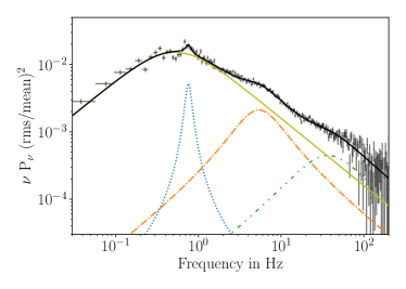
Figure 1: Power density spectrum of MAXI J1820+070 as observed by NICER for the observation ID 1200120161. The PDS is normalised to fractional rms squared units after subtraction of Poissonian noise. For plotting purpose, we have multiplied the power with the frequency to highlight the position of the characteristic frequencies of different components. The PDS was modelled using Lorentzian function (individual components are shown in different colours). The detected QPO is shown as blue dotted line while the associated broad noise components are shown as yellow solid, orange dash-dotted and green dash-double dotted lines respectively.

A subset of the hard state observations show a prominent low frequency QPO. The detections of the QPO are also reported in Stiele & Kong (2020) and Mudambi et al. (2020). Stiele & Kong (2020) have detected and reported a pair of QPOs throughout the NICER observations with varying quality factors and significance. The pair of the QPOs are harmonically linked harmonically linked and the higher frequency QPO typically is more significant. In our analysis, we model only the higher frequency QPO as it is stronger and the addition of the lower frequency QPO did not change the fit statistic significantly. The observations which show the QPO have been tabulated in Table 1 along with the observed QPOs and the characteristic frequencies of the higher broad noise components. To compare with the previous works (e.g. Belloni et al., 2002; Motta et al., 2014a; Motta et al., 2014b), we label the detected QPOs as $\nu_{\rm{LT}}$ and the lowest, middle and higher broad noise components as $\nu_{\rm{B}}$, $\nu_{\rm{L}}$ and $\nu_{\rm{U}}$ respectively. The variation of the QPOs and other components is shown in Figure 2. The QPOs detected by Stiele & Kong (2020) and this work match within the 1$\sigma$ confidence interval. These observations also show broad noise components similar to the ones observed in Psaltis et al. (1999), Belloni et al. (2002), Motta et al. (2014a) and Motta et al. (2014b). The frequencies at which these broad features peak in the $\nu\rm{P}_{\nu}$ plot (also known as the characteristic frequency; $\nu_{\rm{char}}=\sqrt{\nu_{\rm{c}}^{2}+(w/2)^{2}}$, Belloni et al., 2002) and the QPO frequency are correlated with each other (see figure 2). We also plot $\nu_{\rm{char}}$ of different components with the QPO frequency in figure 3 to highlight the correlation of all the frequencies.

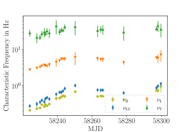
Figure 2: The evolution of the characteristic frequencies of different components is shown here. The colour scheme of the components is kept identical to Figure 1. The $1\sigma$ error bars are also indicated for all the frequencies.

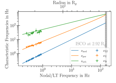
Figure 3: The correlation between the characteristic frequencies of different components with $\nu_{\rm{LT}}$ is shown here. The colour scheme of the points is kept consistent with features observed in Figures 1 and 2. The correlation of the blue points (i.e. $\nu_{\rm{LT}}$) is artificial as the same points are plotted with each other. The solid lines correspond to the frequencies predicted by the best fit RPM. The vertical dashed line corresponds to the highest QPO frequency that can be expected for the assumed mass and estimate spin of the source. The grey band corresponds to the 1$\sigma$ confidence interval on the highest QPO frequency.

Table 1: Summary of the QPOs and broad noise features used to constrain the spin of the source. The error bars reported here correspond to 1$\sigma$ confidence interval.

Observation ID	Start MJD	$\nu_{\rm{LT}}$ (Hz)	$\nu_{\rm{L}}$ (Hz)	$\nu_{\rm{U}}$ (Hz)
1200120130	58224.068	$0.276\pm 0.021$	$2.79\pm 0.09$	$29.2\pm 6.1$
1200120132	58228.124	$0.315\pm 0.051$	$3.12\pm 0.18$	$22.0\pm 6.8$
1200120134	58229.984	$0.353\pm 0.035$	$3.32\pm 0.12$	$22.2\pm 3.6$
1200120135	58231.032	$0.400\pm 0.031$	$3.56\pm 0.20$	$27.8\pm 5.3$
1200120136	58232.452	$0.362\pm 0.014$	$3.77\pm 0.37$	$30.7\pm 8.7$
1200120137	58233.026	$0.438\pm 0.043$	$3.69\pm 0.18$	$27.8\pm 4.2$
1200120138	58233.991	$0.473\pm 0.031$	$3.52\pm 0.23$	$33.0\pm 6.9$
1200120139	58235.339	$0.431\pm 0.039$	$3.86\pm 0.47$	$29.2\pm 8.3$
1200120141	58239.314	$0.587\pm 0.038$	$4.50\pm 1.10$	$45.4\pm 19$
1200120143	58241.246	$0.664\pm 0.029$	$4.97\pm 0.43$	$31.8\pm 6.5$
1200120144	58242.275	$0.664\pm 0.016$	$5.61\pm 0.43$	$35.2\pm 5.4$
1200120145	58243.242	$0.722\pm 0.024$	$5.60\pm 0.45$	$34.7\pm 4.2$
1200120146	58244.276	$0.842\pm 0.055$	$5.58\pm 0.63$	$42.7\pm 7.4$
1200120152	58250.255	$1.023\pm 0.070$	$6.14\pm 2.41$	$43.5\pm 18$
1200120159	58263.209	$0.769\pm 0.040$	$5.65\pm 0.88$	$34.2\pm 12$
1200120161	58265.064	$0.758\pm 0.042$	$5.39\pm 0.62$	$37.2\pm 8.1$
1200120162	58266.217	$0.762\pm 0.024$	$5.41\pm 0.84$	$36.4\pm 11$
1200120174	58278.263	$0.636\pm 0.025$	$4.41\pm 0.58$	$30.7\pm 13$
1200120189	58297.194	$0.875\pm 0.013$	$6.08\pm 0.59$	$38.0\pm 5.6$
1200120190	58298.028	$0.989\pm 0.028$	$5.81\pm 1.55$	$46.3\pm 15$
1200120191	58299.752	$1.143\pm 0.062$	$7.22\pm 2.55$	$36.8\pm 15$

As seen in Motta et al. (2014a) and Motta et al. (2014b), the characteristic frequencies of the broad features follow the trend predicted by RPM, although with a significant scatter. Such a scatter is likely related to the fact that the physics of the accretion flow is more complex than that assumed by the RPM, as well as to a more practical reason, namely that the characteristic frequency of a broad PDS component is not an obvious measurable, and the definition we assumed might not be accurate enough. The implication of the above will be discussed in Sec. 3. In principle, one could use triplets formed by two broad PDS components (associated with the high-frequency QPOs, see Psaltis et al. 1999 and Motta et al. 2014a and a low-frequency QPO to constrain the mass and spin of a BH. However, given the presence of a large scatter, using triplets individually could yield inconsistent values of the mass and spin. In order to mitigate the effects of the scatter, we can fit the trend followed by the frequencies to determine the optimal parameters of the BH, which will be therefore estimated based on the overall correlation, rather than on individual (possibly biased) points. Using optical observations and jet inclination, Torres et al. (2020) have determined the mass of the source which we have used as an input. Using the equation of nodal precession frequency from Motta et al. (2014a), we solve for the radius of oscillation for an assumed spin of the black hole using the Newton-Raphson method. We compute the frequency of the periastron precession and orbital oscillation frequency using the equations from Motta et al. (2014a) at that radius. We compute the $\chi^{2}$ between the model frequencies and the characteristic frequencies of the observed broad noise components. Since individual detections of frequencies are independent, we summed the $\chi^{2}$ from each observation to obtain a total $\chi^{2}$. Varying the spin as a parameter, we determine the spin of the source where the total $\chi^{2}$ is found to be minimum. The variation of the total $\chi^{2}$ with the spin is shown in Figure 4. We repeated the process for different mass values indicated by the 1$\sigma$ confidence interval from Torres et al. (2020). The correlation in Figure 3 is also overplotted with the predicted RPM frequencies for the assumed mass and the computed spin. The radius of oscillation corresponding to the QPO is shown in the top axis of Figure 3.

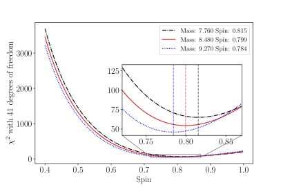
Figure 4: Variation of total $\chi^{2}$ with the spin for different assumed masses of the source. The choice of masses is from the current mass estimate of the source from Torres et al. (2020) and corresponds to the 1$\sigma$ lower limit (shown in black dot dashed line), best guess (shown in red solid line) and 1$\sigma$ upper limit (shown in blue dotted line). The inset shows variation near the minima of the $\chi^{2}$ and vertical dashed lines indicate the minimum of each assumed mass. The predicted spin values for each mass is reported in the legend.

We find that the $\chi^{2}$ is minimum (54.354 for 41 degrees of freedom) for the spin value of 0.799 when the assumed mass is 8.48 M_⊙ (central value in the interval of Torres et al., 2020). The lowest $\chi^{2}$ for the lower and upper limit of mass interval from Torres et al. (2020) corresponds to a spin of 0.815 and 0.784 respectively. The uncertainty on the spin measurement from the $\chi^{2}$ distribution is lower that the one propagated from the mass confidence interval by an order of magnitude and thus we report the uncertainty in spin as determined from the error propagation from the mass confidence interval. We also determine the variation of the $\chi^{2}$ as a function of both mass and spin. Assuming the likelihood as determined from the $\chi^{2}$ method, we apply a uniform prior on mass and spin. For spin we allow for complete range i.e. -0.998 to 0.998 and for mass we first assume the uniform prior spanning 1$\sigma$ interval from Torres et al. (2020) and then we assume an extremely conservative uniform prior of 5–20 M_⊙. We used Markov-Chain Monte Carlo sampling using emcee package (Foreman-Mackey et al., 2013) by initialising 150 walkers around a narrow interval around the guess mass and spin of 8.48 M_⊙ and 0.8 respectively. The walkers were allowed to move 1500 steps individually and initial 200 steps were discarded to remove the effects of initialisation. As a second test, we apply a Gaussian prior on the mass assuming a mean of 8.48 M_⊙ and a standard deviation of 0.7 M_⊙ (as suggested by Torres et al., 2020) We have plotted the 2-D probability distribution of mass and spin and the marginalised distributions of mass and spin for both cases in Figure 5. The spin measurement for a fixed mass of 8.48 M_⊙ is indicated as a black point in the top panel.

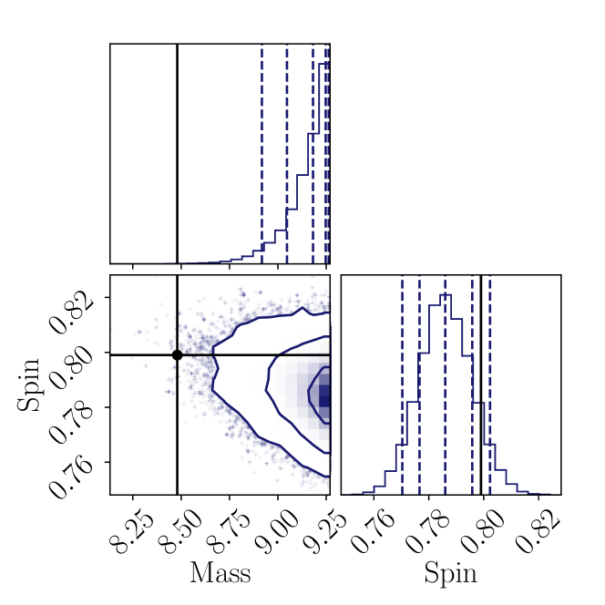
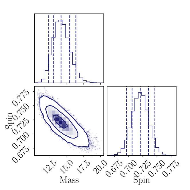
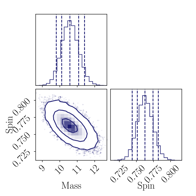
Figure 5: Corner plots for MCMC sampling of parameter space. The top panel considers a uniform prior over 1$\sigma$ confidence interval from Torres et al. (2020). The black point indicates the spin estimate from the $\chi^{2}$ minimisation for assumed mass. The middle plot considers a uniform prior over a wide mass range of 5–20 M_⊙ while the bottom plot assumes a Gaussian prior on mass with 8.48 M_⊙ as mean and 0.7 M_⊙ as the standard deviation. In all three cases the spin is drawn from a uniform distribution ranging from -0.998 to 0.998.

3 Results and Discussion

We used observations of the BHB MAXI J1820+070 with NICER to study the variation of the timing properties of the source. The PDS of the source showed significant broadband noise in 0.03–100 Hz. Some of the observations also show a type-C QPO (typically $<$1 Hz). These observations also show broadband noise features at higher frequencies which correlate with the evolution of the QPO as seen in other X-ray binaries (Psaltis et al., 1999; Belloni et al., 2002; Motta et al., 2014a; Motta et al., 2014b).

We fit the observed QPO and the characteristic frequencies of the broad noise features to the Relativistic Precession model. We use the mass of the BH inferred from the spectro-photometric optical observations to put tight constraints on the spin of the source. We derive a spin of the source of $0.799^{+0.016}_{-0.015}$. The ISCO corresponding to this spin is 2.91 R_g. The low frequency QPOs corresponds to large radii of oscillation (15–25 R_g, see Figure 3). Allowing the mass and spin to vary simultaneously, the mass of the source is overestimated, as compared to Torres et al. (2020) measurement, by a factor of 1.2 or 1.6 (depending on the choice of prior on the mass, Gaussian or Uniform). For the overestimated mass, the corresponding spin estimate is reduced to 0.76 or 0.72 respectively. Restricting the mass to 1$\sigma$ confidence interval suggested by Torres et al. (2020) prefers a 9.25 M_⊙ BH with a spin of 0.78.

3.1 RPM and broad components

Psaltis et al. (1999) have associated the broad noise components as the low frequency counterparts of the HFQPOs. Motta et al. (2014a) and Motta et al. (2014b) have observed a similar trend for GRO J1655$-$40 and XTE J1550$-$564 respectively. The broad components are observed simultaneously with a low frequency type-C QPO ($\leq$1 Hz), which occur at a larger radius. In XTE J1550$-$564, some of the RXTE observations show the presence of broad components which match the predicted periastron precession and orbital frequencies motivating the hypothesis that the broad features are indeed the low frequency counterparts. The broad components in these sources have shown a scatter around the trend predicted by RPM. In NICER observations of MAXI J1820+070, we see a similar phenomenon, which has motivated us to use RPM to describe the observed frequencies. Motta et al. (2014b) discusses the possible reasons for the scatter of the broad noise components. The broad components are associated with the oscillations arising at a larger radii and at these radii the test particle orbits might differ substantially from the accretion orbits. The scatter between the components can also arise from the assumptions in the modelling of these features.

While the mass posterior we recover is consistent with the mass value obtained by Torres et al. (2020), the central mass is significantly larger than the best value reported by such authors. This effect might be due to a bias introduced by the fact that in this work we consider broad PDS components rather than QPOs, which do not provide a clear centroid frequency. According to the PBK relation (Psaltis et al., 1999), certain broad components in the PDS are associated to HFQPOs when these are generated at large distances from the central BH. By fitting large PDS components with the RPM, rather than narrow HFQPOs (which are instead assumed to be generated at small radii from the BH) results are much more affected by the effects of matter precessing as part of an extended disc (Motta et al., 2018). On the one hand, adopting the RPM at large radii, one models an extended disc assuming it is a narrow precessing ring. This implies that the radii are assumed to be smaller than they really are (for a given radius, the extended disc precession frequency is larger than a ring precession frequency). This induces a shift to higher masses (and smaller spins), which counterbalances the bias in radius. On the other hand, as one considers wider and wider orbits, the torque exerted by the outer disc on a particle on a given orbit grows larger compared to the torque exerted by the frame dragging, so that precession might be slowed down. This means that what is actually measured is a precession frequency slower than expected, which once more induces a shift towards larger masses. These two effects combined might effectively push the posterior distribution to higher masses.

3.2 Spin measurement

The ISCO corresponding to spin of 0.8 is 2.91 R_g, which allows for a truncated inner disk at $\sim$5 R_g (Bharali et al., 2019; Buisson et al., 2019). In their analysis, Bharali et al. (2019) found that the broadband spectra is consistent with a maximal spinning BH with a lower limit of 0.68, which is consistent with our measurements. The observation of inner truncated disk at the 5.3 R_g is interpreted as the ISCO by Buisson et al. (2019) which corresponds to a low spin but in the hard state of BHBs, the accretion disk is typically truncated and need not correspond to ISCO (Done et al., 2007). Fabian et al. (2020) have reported a strong degeneracy between the spin and inclination measurement. A high inclination of the source (from radio measurements Atri et al., 2020) would correspond to a retrograde spin of the black hole while a lower inclination ($\sim 30^{\circ}$ Bharali et al., 2019; Buisson et al., 2019) of the source supports a high prograde spin. A retrograde spin is quite inconsistent with the measured inner truncation radius of $\sim 5$ R_g. On the other hand, our spin measurement would imply that the inclination of the disk is closer to $30^{\circ}$ and indicate a possible misalignment between the inner disk inclination and the jet inclination (Miller-Jones et al., 2019). The spectral continuum modelling in the soft state of the source by Guan et al. (2020) yields a low spin of the source which we note significantly differs from our measurement. The continuum modelling method assumes that the inner truncation is reaching the ISCO which is unconfirmed. The measured inner truncation can thus only provide a lower limit on the spin of the source and is still consistent with a high spin measurement.

As indicated in the previous section, the method overestimates the mass of the BH due to the interpretation of the broad features arising from a narrow ring. The overestimation of the mass implies an underestimation of the spin as indicated by the contours in figure 5. Even with fixing the mass at 8.48 M_⊙, the estimated spin of 0.799 may be regarded as a lower limit owing to the assumption that the broad noise features behave strictly according to the RPM. The quantification of the bias inherent in this method will be followed up in a future work.

3.3 Disk truncation

The measurement of the inner disk truncation from the spectroscopic measurements vary significantly as different accretion models have different inherent geometrical and physical assumptions leading to the discrepancy. Most of the works have analysed the hard or hard-intermediate state observations making it easier to compare and track the evolution. Dziełak et al. (2021) utilise the hard state observation and place the inner truncation radius at 45 R_g using the temperature constraints from the frequency resolved spectrum. In contrast Bharali et al. (2019) determine the inner truncation radius of the source at 5.1 R_g at a similar epoch. Buisson et al. (2019) have analysed the hard and hard-intermediate state observations and have observed a truncation at 5.3 R_g, while Zdziarski et al. (2021) and De Marco et al. (2021) suggests that in the hard and hard intermediate states, the inner truncation of the disk is $\gtrsim$10 R_g. The observations we have analysed in the present work correspond to hard intermediate states stopping a few days prior to the state transition discussed in Homan et al. (2020) and De Marco et al. (2021). The special radius at which QPO is arising, as suggested by the RPM, varies within 15–25 R_g. This radius although inconsistent with the truncation radius from spectral measurements assuming a lamppost geometry (Bharali et al., 2019; Buisson et al., 2019), is allowed by alternative geometries (De Marco et al., 2021; Zdziarski et al., 2021; Dziełak et al., 2021). In these geometries, the special radius at which QPO is arising could correspond to a transition region to a hot accretion plasma (Dziełak et al., 2021) or could indicate the extent of covering by the comptonising medium (Zdziarski et al., 2021).

4 Conclusions

Using the RPM, we provide an estimate of the spin of the source at 0.799 ${}^{+0.016}_{-0.015}$ for an assumed mass of the source at 8.48 M_⊙. Exploring a wider parameter space indicates that the method is sensitive to assumption of the priors on the mass and for uninformative priors, the method prefers a mass higher than the one estimated by optical measurements and a slightly lower spin. However, we argue that the use of broad features instead of QPO peaks in the analysis of the Relativistic Precession Model tends to introduce a bias so as to underestimate the spin and overestimate the mass. The estimated spin quoted above should therefore be regarded as a lower limit.

Data Availability

The data underlying this article are available in https://heasarc.gsfc.nasa.gov/docs/archive.html using the observation IDs listed in Table 1. The associated software to process the data are also available publicly at the same. TMB can be contacted for GHATS.

References

- Abramowicz & Kluźniak (2001) Abramowicz M. A., Kluźniak W., 2001, A&A, 374, L19
- Atri et al. (2020) Atri P., et al., 2020, MNRAS, 493, L81
- Belloni & Hasinger (1990) Belloni T., Hasinger G., 1990, A&A, 227, L33
- Belloni & Motta (2016) Belloni T. M., Motta S. E., 2016, Transient Black Hole Binaries. p. 61, doi:10.1007/978-3-662-52859-4_2
- Belloni et al. (1999) Belloni T., Méndez M., van der Klis M., Lewin W. H. G., Dieters S., 1999, ApJ, 519, L159
- Belloni et al. (2002) Belloni T., Psaltis D., van der Klis M., 2002, ApJ, 572, 392
- Belloni et al. (2005) Belloni T., Homan J., Casella P., van der Klis M., Nespoli E., Lewin W. H. G., Miller J. M., Méndez M., 2005, A&A, 440, 207
- Bharali et al. (2019) Bharali P., Chauhan J., Boruah K., 2019, MNRAS, 487, 5946
- Buisson et al. (2019) Buisson D. J. K., et al., 2019, MNRAS, 490, 1350
- Buisson et al. (2021) Buisson D. J. K., et al., 2021, MNRAS, 500, 3976
- Casella et al. (2005) Casella P., Belloni T., Stella L., 2005, ApJ, 629, 403
- Chakraborty et al. (2020) Chakraborty S., Navale N., Ratheesh A., Bhattacharyya S., 2020, MNRAS, 498, 5873
- De Marco et al. (2021) De Marco B., Zdziarski A. A., Ponti G., Migliori G., Belloni T. M., Segovia Otero A., Dziełak M., Lai E. V., 2021, arXiv e-prints, p. arXiv:2102.07811
- Done et al. (2007) Done C., Gierliński M., Kubota A., 2007, A&ARv, 15, 1
- Dziełak et al. (2021) Dziełak M. A., De Marco B., Zdziarski A. A., 2021, arXiv e-prints, p. arXiv:2102.11635
- Fabian et al. (2020) Fabian A. C., et al., 2020, MNRAS, 493, 5389
- Foreman-Mackey et al. (2013) Foreman-Mackey D., Hogg D. W., Lang D., Goodman J., 2013, PASP, 125, 306
- Gandhi et al. (2019) Gandhi P., Rao A., Johnson M. A. C., Paice J. A., Maccarone T. J., 2019, MNRAS, 485, 2642
- Gendreau et al. (2016) Gendreau K. C., et al., 2016, The Neutron star Interior Composition Explorer (NICER): design and development. p. 99051H, doi:10.1117/12.2231304
- Guan et al. (2020) Guan J., et al., 2020, arXiv e-prints, p. arXiv:2012.12067
- Homan et al. (2020) Homan J., et al., 2020, ApJ, 891, L29
- Ingram & Motta (2020) Ingram A., Motta S., 2020, arXiv e-prints, p. arXiv:2001.08758
- Kara et al. (2019) Kara E., et al., 2019, Nature, 565, 198
- Kawamuro et al. (2018) Kawamuro T., et al., 2018, The Astronomer’s Telegram, 11399, 1
- Kennea et al. (2018) Kennea J. A., Marshall F. E., Page K. L., Palmer D. M., Siegel M. H., Neil Gehrels Swift Observatory Team 2018, The Astronomer’s Telegram, 11403, 1
- Leahy et al. (1983) Leahy D. A., Darbro W., Elsner R. F., Weisskopf M. C., Sutherland P. G., Kahn S., Grindlay J. E., 1983, ApJ, 266, 160
- McKinney et al. (2012) McKinney J. C., Tchekhovskoy A., Blandford R. D., 2012, MNRAS, 423, 3083
- Miller-Jones et al. (2019) Miller-Jones J. C. A., et al., 2019, Nature, 569, 374
- Miller et al. (2009) Miller J. M., Reynolds C. S., Fabian A. C., Miniutti G., Gallo L. C., 2009, ApJ, 697, 900
- Motta et al. (2014a) Motta S. E., Belloni T. M., Stella L., Muñoz-Darias T., Fender R., 2014a, MNRAS, 437, 2554
- Motta et al. (2014b) Motta S. E., Munoz-Darias T., Sanna A., Fender R., Belloni T., Stella L., 2014b, MNRAS, 439, L65
- Motta et al. (2018) Motta S. E., Franchini A., Lodato G., Mastroserio G., 2018, MNRAS, 473, 431
- Mudambi et al. (2020) Mudambi S. P., Maqbool B., Misra R., Hebbar S., Yadav J. S., Gudennavar S. B., S. G. B., 2020, ApJ, 889, L17
- Nowak et al. (1997) Nowak M. A., Wagoner R. V., Begelman M. C., Lehr D. E., 1997, ApJ, 477, L91
- Psaltis et al. (1999) Psaltis D., Belloni T., van der Klis M., 1999, ApJ, 520, 262
- Remillard & McClintock (2006) Remillard R. A., McClintock J. E., 2006, ARA&A, 44, 49
- Reynolds (2020) Reynolds C. S., 2020, arXiv e-prints, p. arXiv:2011.08948
- Reynolds & Miller (2009) Reynolds C. S., Miller M. C., 2009, ApJ, 692, 869
- Shidatsu et al. (2018) Shidatsu M., et al., 2018, ApJ, 868, 54
- Shidatsu et al. (2019) Shidatsu M., Nakahira S., Murata K. L., Adachi R., Kawai N., Ueda Y., Negoro H., 2019, ApJ, 874, 183
- Stella & Vietri (1998) Stella L., Vietri M., 1998, ApJ, 492, L59
- Stella et al. (1999) Stella L., Vietri M., Morsink S. M., 1999, ApJ, 524, L63
- Stiele & Kong (2020) Stiele H., Kong A. K. H., 2020, ApJ, 889, 142
- Strohmayer (2001) Strohmayer T. E., 2001, ApJ, 552, L49
- Torres et al. (2019) Torres M. A. P., Casares J., Jiménez-Ibarra F., Muñoz-Darias T., Armas Padilla M., Jonker P. G., Heida M., 2019, ApJ, 882, L21
- Torres et al. (2020) Torres M. A. P., Casares J., Jiménez-Ibarra F., Álvarez-Hernández A., Muñoz-Darias T., Armas Padilla M., Jonker P. G., Heida M., 2020, ApJ, 893, L37
- Zdziarski et al. (2021) Zdziarski A. A., Dziełak M. A., De Marco B., Szanecki M., Niedźwiecki A., 2021, ApJ, 909, L9