Systemic risk in interbank networks:
disentangling balance sheets and network effects

We study the difference between the level of systemic risk that is empirically measured on an interbank network and the risk that can be deduced from the balance sheets composition of the participating banks.Using generalised DebtRank dynamics, we measure observed systemic risk on e-MID network data (augmented by BankFocus information) and compare it with the expected systemic risk of a null model network – obtained through an appropriate maximum-entropy approach constraining relevant balance sheet variables. We show that the aggregate levels of observed and expected systemic risks are usually compatible but differ significantly during turbulent times – in our case, after the default of Lehman Brothers (2009) and the VLTRO implementation by the ECB (2012). At the individual level instead, banks are typically more or less risky than what their balance sheet prescribes due to their position in the network. Our results confirm on one hand that balance sheet information used within a proper maximum-entropy network model provides good aggregate estimates of systemic risk, and on the other hand the importance of knowing the empirical details of the network for conducting precise stress tests on individual banks – especially after systemic events.

Keywords: Financial networks; Interbank market; Network theory; Systemic risk; Contagion

JEL Codes: G01, G21, G33, C49, C63

1 Introduction

Research about contagion in financial networks has attracted much interest in the last twenty years (Bougheas and Kirman,, 2015; Huser,, 2015; Battiston et al.,, 2016; Glasserman and Young,, 2016; Gai and Kapadia,, 2019; Bardoscia et al.,, 2021; Jackson and Pernoud,, 2021), particularly after the Global Financial Crisis of 2007/08 (GFC). A key driver has been the request by regulators and policymakers for a deeper understanding of how the issue of interconnectedness can influence systemic risk and financial stability (Haldane,, 2009; Yellen,, 2013).

While systemic risk can arise in several contexts (Benoit et al.,, 2017), much attention has been devoted to interbank networks – defined by considering each loan among two banks as a directed link between the lender and the borrower and thus translating the balance sheet structure into a network. When a shock hits one or more banks, the network structure allows the shock to propagate to neighbouring institutions, potentially amplifying its effects. The literature has thus focused on understanding the dynamics of the contagion process, quantifying the probability and extent of a systemic event, and overall assessing how the stability of the system changes with the structure of the network.

Empirical research addressed interbank contagion even before the GFC. Using the algorithms created by Eisenberg and Noe, (2001) and Furfine, (2003), several studies analysed the possible effects of contagion on real or estimated networks in US (Furfine,, 2003), UK (Wells,, 2004; Elsinger et al.,, 2005), Austria (Elsinger et al.,, 2006), Brazil (Cont et al.,, 2010) and Italy (Mistrulli,, 2011). In his review, Upper, (2011) concluded that the risk of contagion should be taken seriously because a systemic event, even if rare, could affect a substantial part of the banking system. A more recent methodology to address financial contagion is the DebtRank algorithm (Battiston et al., 2012b, ; Bardoscia et al.,, 2015), further generalised by Barucca et al., (2020) into the NEVA (Network Valuation of Financial Assets) framework.

From the theoretical point of view, pioneers in this kind of analysis were Allen and Gale, (2000) and Freixas and Parigi, (2000). Allen and Gale, (2000) considered a model in which regional banks are connected through interbank transactions and are subject to non-perfectly correlated deposit withdrawals. Even if their model is small and unrealistic, they showed that contagion is highly dependent on the network structure, with the complete network perfectly spreading the shock over the entire system and the ring network being the most fragile topology. In a similar setting, Freixas and Parigi, (2000) concluded that more links increase the resiliency of the system by increasing its ability to absorb shocks.

Recent advancement on the topic was given by Acemoglu et al., (2015). They showed that the financial system displays a ”robust-yet-fragile” structure: for small shocks, a denser network increases the resiliency, thereby confirming the results of Allen and Gale, (2000) and Freixas and Parigi, (2000); for shocks over a certain threshold instead, increasing the density of the network increases its fragility. Previous evidence of the non-monotonic effects of the connectivity was provided by Gai and Kapadia, (2010). Using Erdős–Rényi random graphs, they showed that the probability of contagion changes non-monotonically with the average degree of the network: before a certain threshold, growth in connectivity has risk-spreading effects whereas, over that threshold, risk-sharing effects prevail. Similarly, Battiston et al., 2012a found that individual diversification has ambiguous effects on the size of the default cascades – depending on the distribution of banks’ robustness, the size of the initial shock, and the presence of runs.

Other studies used DebtRank to analyse which are the topological aspects of a network that drive the level of systemic risk. Bardoscia et al., (2017) showed that increments in the network density increase instability, the reason being the presence of more cycles that act as risk amplifiers. Ramadiah et al., (2020) showed that the dependence of systemic risk on the network density also depends on the functional form of the contagion. They further considered block-structured networks, showing that risk is higher in marked core-periphery topologies due to the presence of a strongly connected set of banks that enhance the contagion process.

Although all these studies analyse which characteristics make the stability of interbank networks vary, there is no empirical research that tries to disentangle between the risk that is inherent to the balance sheet structure of the system and to the link density of the network, which we term expected systemic risk, and what is generated by the other specific topological features of the network at hand. The aim of this study is precisely to address this point. To this end, we compare the systemic risk indicators measured on a real interbank network with those computed within an ensemble of null models that satisfy the same balance sheets of the data and whose links represent possible clearing configurations for the market. In order to generate the null networks, we introduce the Separable Directed Enhanced Configuration Model (SDECM), a maximum-entropy construction that preserves the in/out-degree and in/out-strength of each bank – respectively, the number of counterparties and the total amount of interbank assets and liabilities – representing the relevant balance sheet variables. Thanks to this procedure, we can compute the level of systemic risk that is expected given the empirical balance sheets constraints and the observed level of connectivity in the system, and that is not due to a specific network configuration.

We measure the systemic risk of the whole market and the systemic relevance of individual institutions using the NEVA framework (Barucca et al.,, 2020) with the valuation functions that are frequently used in the literature: DebtRank (both in its linear and nonlinear form) and Furfine. Our data consists of interbank exposures from the electronic Market of Interbank Deposits (e-MID). Since this data does not include information about the equity of the institutions participating in the market, we estimate the relation between interbank positions and equity using data from BankFocus, and exploit this relation to augment e-MID data.

Our results show that using only the information from balance sheets is typically not enough to monitor the interbank network’s stability. Indeed while the aggregated systemic risk for all banks in the market is usually compatible with its expected value, significant deviations appear during turbulent times – namely, the failure of Lehman Brothers (2009 network) and the introduction of the 3-year LTRO (2012 network). Instead, the knowledge of the exact position of a bank in the network is always required to assess its systemic importance. Also in the granular analysis the largest deviations are observed in 2009 and 2012.

In 2009, the observed systemic risk is lower than what is implied by the balance sheets composition. This observation is in line with the literature on interbank markets during the GFC (Angelini et al.,, 2011; Afonso et al.,, 2011; Affinito and Pozzolo,, 2017), showing that banks had increased concerns about counterparty risk, in particular after the Default of Lehman Brothers. On the contrary, in the 2012 network we observe positive deviations which we argue are generated by the introduction of the 3-year LTRO. These operations had a profound impact on interbank markets (Affinito and Pozzolo,, 2017; Barucca and Lillo,, 2018) and probably decreased banks’ risk aversion, consistently with the risk-taking channel of monetary policy (Borio and Zhu,, 2008).

Overall, our results underline the importance of using network models and collecting data to precisely monitor contagion effects and thus ensure financial stability. Using only balance sheet information is not enough, especially when it matters the most — that is when disruptive events are at play. Supervisors and policy maker should thus continue with their efforts in monitoring the network structure of the market and using network models for stress testing the financial system.

Closely related to our study are the ones of Krause et al., (2019) and Diem et al., (2020), both based on DebtRank. Using Monte Carlo network generation, Krause et al., (2019) showed that it is possible to create financial networks with minimal systemic risk while maintaining fixed balance sheet structures. Another significant result of their analysis is that it is possible to derive approximate information about the systemic risk of a financial institution by using specific node properties, notably the interbank leverage. Diem et al., (2020) also performed a systemic risk optimisation through mixed-integer linear programming: They fixed interbank assets and liabilities and optimised the network structure to obtain minimal systemic risk. They showed that sensible risk reductions are possible, especially for small and medium-sized banks, by concentrating lending and funding over a minimal set of connections.

Our study differs from both these works since, in our exercise, we also fix the degrees of each institution: banks’ diversification is kept constant, and thus concentration limits are respected. We also have a different goal: we do not aim to find the network structure of minimal systemic risk, but we aim to quantify the systemic risk expected from a given set of heterogeneous balance sheets and diversification strategies. By fixing the size of the interbank exposures and the level of interconnectedness, we aim to measure the contribution of the observed pattern of links while controlling for variables that are known to have large effects on the risk of contagion.

Another closely related study is Glasserman and Young, (2015), who derive explicit bounds for the magnitude of network contagion while using only minimal information about the connectivity of the network. Their method allows to compute the maximum systemic risk generated by a shock with only data about asset size, leverage and total interbank liabilities and does not need exact knowledge about the underlying network structure. There are several significant differences between their approach and ours. First, their model does not use information about the number of counterparties of each bank, while our measures take into account this information. Second, their analysis is model-dependent, as it relies on the Eisenberg-Noe framework; on the contrary, our approach can be applied to any existing model. Third, their measure allows to compute the maximum systemic risk generated by an interbank network rather than the expected one.

Moreover, they measure the contribution of the network structure by comparing this bound with a network-less system. On the contrary, in our analysis, we study the difference between the observed networks and the average of an ensemble of fictional networks. Our results regarding the contribution of the specific network structure are comparable to their analysis in the case of a contagion-at-default algorithm. Conversely, when the model entails distress contagion, relevant differences arise.

2 Data and Methodology

2.1 Data

Data on interbank exposures are usually confidential and thus not easily accessible. To obtain a proxy of interbank relationships, we use data from the electronic Market of Interbank Deposits (e-MID), an electronic platform for interbank loans. The data collects information about every transaction from 2005Q1 to 2012Q3, but we restrict the analysis to overnight loans that account for roughly 98% of the total volume. Finger et al., (2013) showed that in order to have information about the underlying ”latent” network of preferential lending relationships, data must be aggregated at least to the monthly level. For consistency with the other data source used in the paper (see below), we decided to aggregate data at the yearly level by summing up all interbank loans between two counterparties in a given year.

We describe the network created from such yearly data using the following notation. During a given year, we have a set of $n$ banks operating in the market, each corresponding to a node of the network. Each gross loan from bank $i$ to bank $j$ will be represented by a directed weighted link $A_{ij}$ connecting the two nodes $i$ and $j$. These links are grouped into a $n\times n$ matrix $A$ of interbank exposures. From $A$ we can derive the $n\times n$ adjacency matrix $G$, whose binary element $g_{ij}$ is equal to $1$ if $A_{ij}>0$ and equal to $0$ otherwise. These matrices encode node-specific properties: the out-degree $k_{i}^{out}$ and the in-degree $k_{i}^{in}$

$$k_{i}^{out}=\sum_{j=1}^{n}g_{ij} k_{i}^{in}=\sum_{j=1}^{n}g_{ji}$$ (1)

representing respectively the number of counterparties that are borrowers and lenders of bank $i$, and the out-strength $s_{i}^{out}$ and the in-strength $s_{i}^{in}$

$$s_{i}^{out}=A_{i}=\sum_{j=1}^{n}A_{ij} s_{i}^{in}=L_{i}=\sum_{j=1}^{n}A_{ji}$$ (2)

that represent the total amount of lending and borrowing of bank $i$.

In order to run the contagion dynamics on the network, we also need information about the equity of each bank. Unfortunately, e-MID data does not come with this information; moreover, banks are anonymised in the dataset, hence it is also impossible to take this information from other sources. To solve this limitation, we employed data from BankFocus about the balance sheet compositions of the financial institutions in the Euro area. This data provides yearly information on equity, loans and advances to banks, and deposits from banks between 2005 and 2012 for a set of 2366 financial institutions. Using this data, we performed, for each year, a simple linear regression between the logarithm of equity and the logarithm of the average between interbank assets and liabilities. In fact, these two variables show a strong linear relation, with an average Pearson correlation coefficient of 0.94 and an average $R^{2}$ of 0.88 from the regression. The validity of this relationship is shown in the scatter plot of Figure 1. We then rescaled the e-MID interbank positions to match the BankFocus average and used the parameters obtained from the linear regression to generate a fictional value for the yearly equity of each bank in the network.

Note that the use of fictional equity values does not hinder our analysis since the same equity is used for each bank in both the empirical e-MID network and the null model. In other words, the composition of balance sheets remains the same in the two scenarios, leaving the link pattern as the only changing variable. This allows us to disentangle between the inherent instability of the system due to balance sheets and the risks generated by the observed network configuration. Indeed, we are not interested in the absolute value of systemic risk but in the difference between observed and expected scenarios.

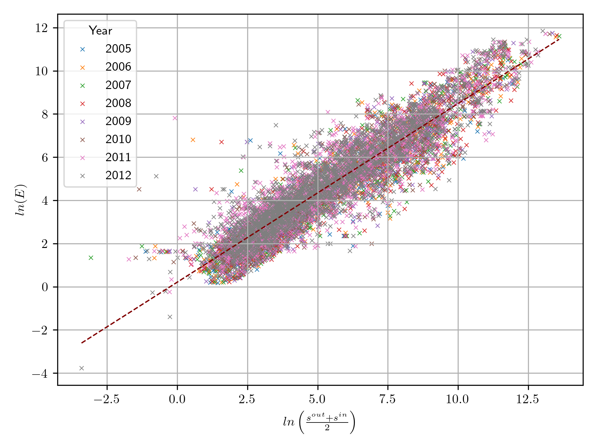
Figure 1: Scatter plot of the yearly logarithmic values of average interbank position and equity for all the banks included in the BankFocus dataset. The dashed line has slope 0.83 and represents the average value obtained by the yearly regressions.

We can finally describe the balance sheet of bank $i$ through the following equation

$$A_{i}+N_{i}^{E}=L_{i}+E_{i}$$ (3)

where $N_{i}^{E}$ represents the total amount of net external assets, computed as the residual of the accounting identity.

2.2 Systemic risk measures

In order to assess the level of systemic risk in the interbank network, we use the NEVA framework (Barucca et al.,, 2020). In the model, after a shock hits the system, each bank re-evaluates its interbank claims and updates the value of its equity accordingly. Subsequently, other rounds of assets valuation are performed until the equity values converge. The iterative map for the equity of each bank can be computed from the balance sheet identity and is the following:

$$E_{i}(t+1)=N_{i}^{E}+\sum_{j=1}^{N}A_{ij}\mathbb{V}(E_{j}(t))-L_{i}$$ (4)

where $\mathbb{V}$ represents the valuation function used to re-evaluate interbank assets, assumed to be homogeneous among all banks, while $t$ stands for the valuation round (that is, the iteration step of the algorithm). The NEVA framework is general enough to encompass different contagion dynamics. In order to compare with previous literature, we use a valuation function that generates contagion on default dynamics, making NEVA equivalent to the Furfine, (2003) algorithm. However, given that the hypothesis of contagion only upon default can be particularly strong, we will also use valuation functions that allow for distress contagion, corresponding to DebtRank both in its linear and nonlinear forms (Bardoscia et al.,, 2015, 2016).

The Furfine algorithm works essentially in three steps. First, a bank $i$ (or a set of banks) fails by assumption. Then contagion propagates through the network, and any other bank $j$ that lent to bank $i$ will suffer a loss $(1-R)A_{ji}$, where $0\leq R<1$ is the recovery rate (i.e., the proportion that the lending bank is able to recover after the default of the counterparty). If $(1-R)A_{ji}>E_{j}$ bank $j$ defaults and a new round of propagation starts. Such dynamics can be obtained in NEVA through the following valuation function:

$$\mathbb{V}_{F}(E_{j}(t))=\mathds{1}_{E_{j}(t)\geq 0}+R\mathds{1}_{E_{j}(t)<0}$$ (5)

where $\mathds{1}$ is an indicator function taking the value of $1$ if the relative condition is met.

According to Furfine dynamics, contagion happens if and only if the equity of a bank in the system drops below zero. This is a strong assumption, as noted by Upper, (2011), also because bank defaults are rare events. Instead, even when no default has occurred, the market value of a loan can drop if the borrower bank is in distress. To model this situation, we use a valuation function compatible with the linear DebtRank dynamics

$$\mathbb{V}_{DR}(E_{j}(t))=min\left[max\left(\frac{E_{j}(t)}{E_{j}(0)},0\right),1\right]$$ (6)

In this case, the equity losses experienced by a bank are always passed to its creditors: each percentage drop of equity is reflected in an equal reduction of interbank claims value.

Finally, we also use a valuation function that maps to the nonlinear DebtRank model

$$\mathbb{V}_{DR(\alpha)}(E_{j}(t))=\left(\mathbb{V}_{[DR]}(E_{j}(t))-1\right)e^{-\alpha\left(\mathbb{V}_{[DR]}(E_{j}(t))-1\right)}+1$$ (7)

In this case, distress is propagated nonlinearly according to the parameter $\alpha$, which sets the functional dependence of the default probability on the relative equity loss: the higher this value, the larger the shock banks can withstand before their probability of default increases. The extreme case $\alpha=0$ corresponds to linear DebtRank and $\alpha\to\infty$ to the Furfine algorithm (see Figure 2).

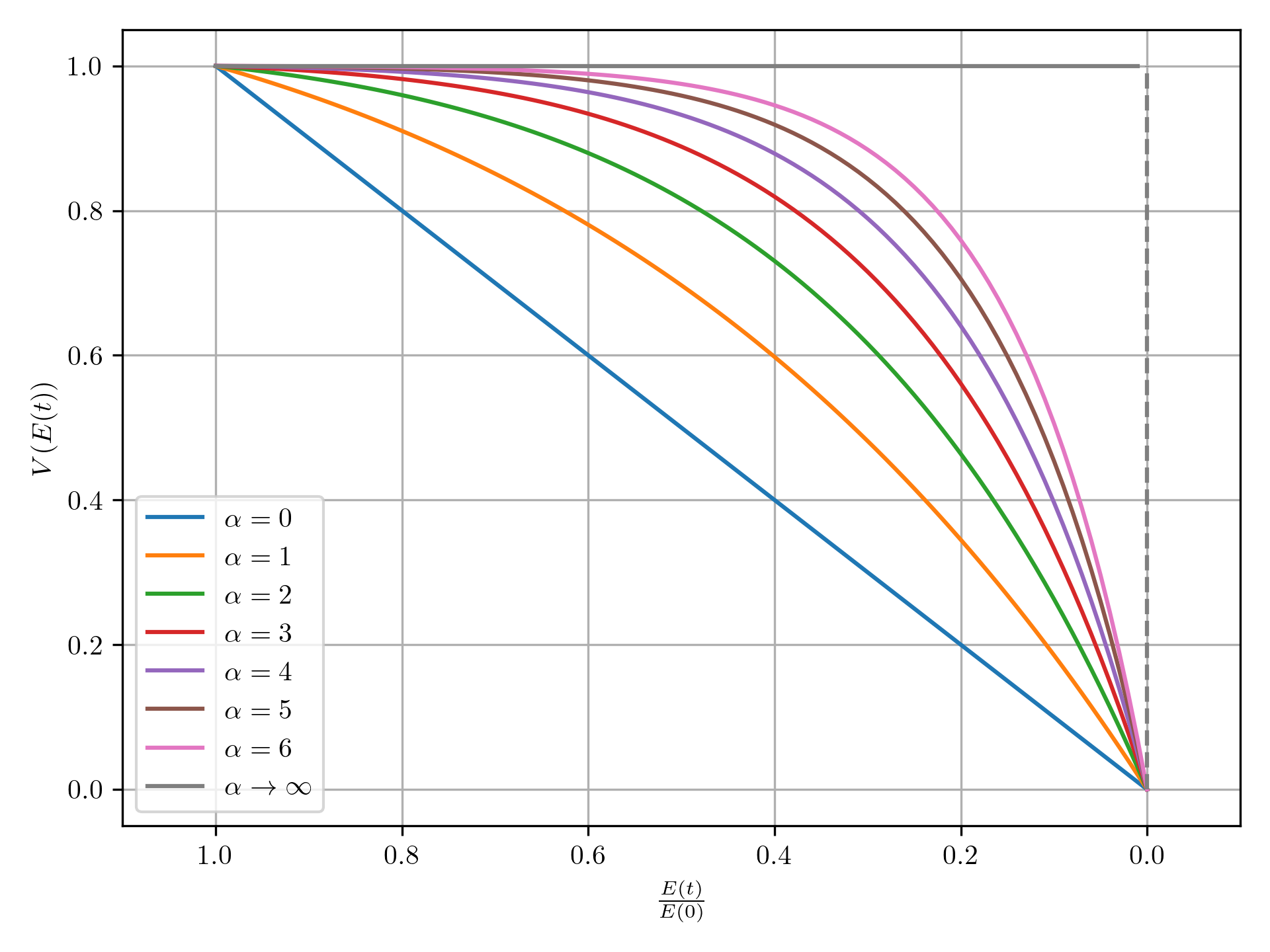
Figure 2: Behaviour of the asset valuation function of eq. (7) in terms of equity loss for the counterparty, for different values of the nonlinearity parameter $\alpha$ ranging from $\alpha=0$ (linear DebtRank) to $\alpha\to\infty$ (Furfine, or contagion on default).

2.3 Null Model

Maximum entropy methodologies derived from Statistical Physics and Information Theory have been mainly used in the field of Economics and Finance to reconstruct networks from a limited set of information due to the confidential nature of financial transactions (see Squartini et al., (2018) for a recent review on the topic). Alternatively, they have been used to perform statistical tests, i.e. to assess the significance of network patterns under specific null hypotheses. Examples of this use are provided by Squartini et al., (2013) and Bargigli et al., (2015), who tested whether the interbank market features an anomalous presence of network motifs that could be interpreted as early warning signs of systemic crises. Using similar methods, Hatzopoulos et al., (2015) tested the e-MID market network for the presence of preferential lending relationships. Other examples are provided by Gualdi et al., (2016) about overlapping portfolios, and Garlaschelli and Loffredo, (2004) about world trade. These models generate an ensemble of networks that are maximally random but on average satisfy some constraints, which are imposed using an entropy maximisation procedure and which thus represent the sufficient statistics of the model (Cimini et al.,, 2019).

In other words, these methods aim at finding the probability distribution that best describes a system when we have only limited information about it. This is achieved by maximising the Shannon entropy (i.e., assuming maximal ignorance on any unknown property) using the available information as constraints. The result is a probability distribution that respects the constrained statistics but where any other property is maximally random.

The aim of this paper is to use a maximum entropy model that allows us to keep fixed the amount of interbank lending and borrowing of each bank together with the level of diversification of each institution. This procedure makes it possible to study the amount of systemic risk that is generated by the specific balance sheet composition of the system while also keeping fixed the level of interconnectedness that, as extensively shown by the literature, deeply affects the outcomes of contagion. This allows measuring the contribution of the specific link structure that has been observed in each yearly network while controlling for the variables that are known to have large effects on systemic risk.

To do so, we introduce the Separable Direct Enhanced Configuration model (SDECM), based on the undirected counterpart by Gabrielli et al., (2019). The model uses as constraints the number counterparties (borrowers $k_{i}^{out}$ and lenders $k_{i}^{in}$) and the total exposure (amounts lent $s_{i}^{out}=A_{i}$ and borrowed $s_{i}^{in}=L_{i}$) in the interbank market for each bank $i$. In order to achieve a good compromise between mathematical rigour and computational efficiency, the model is based on a two-step entropy maximisation procedure: firstly, degree constraints are used to obtain the probability of the adjacency matrix configurations; then, strength constraints are used to obtain the probability density of the link weights conditional to a given binary configuration. The Lagrange multipliers are finally obtained by imposing numerical values of the constraints using likelihood maximisation. For the mathematical details of the model model see Appendix A. Separable Directed Enhanced Configuration Model.

Using SDECM and constraint values taken from the empirical e-MID data, for each year, we generate an ensemble of 1000 networks that shall constitute our null model. With respect to the empirical network, each element in the ensemble has the same number $n$ of banks; on average over this ensemble, each bank has the same number of counterparties and the same total interbank borrowing and lending; apart from satisfying these constraints, transactions between banks and their volumes are placed randomly, such that each network in the ensemble represents a different market configuration. This, plus the use of fixed equity values simulated from BankFocus ensures that the level of interconnectedness and the balance sheets composition of the null model coincides (on average) with that of the empirical network.

We use the contagion model on each generated network to obtain the average and standard deviation values for various systemic risk indicators. We shall refer to these quantities as the expected systemic risk metrics conditional to the balance sheets structure of the market. The comparison of such expected indicators with the ones observed in the real e-MID network allows us to disentangle the risk inherent to the balance sheets with the risk due to the specific configuration of the network.

Furthermore, the SDECM enables us to remain as agnostic as possible with respect to the network formation process of the interbank market. Given that the matching mechanisms of the market are likely changing during the timespan of the data, with the SDECM we assume the simplest formation process, i.e. the one driven by pure randomness. This choice gives us the possibility to observe if banks’ choices of counterparties change throughout our sample and if those different choices entail different levels of systemic risk.

3 Results

We now consider two different settings concerning the initial shock. Firstly in section 3.1 we apply a systemic shock to all banks and analyse the aggregate level of systemic risk. Then in section 3.2 we analyse the systemic relevance of individual banks by letting them default.

3.1 Aggregate systemic risk

We begin our analysis by studying the effect of a small exogenous initial shock distributed on the entire network. This shock is simulated, for each bank $i$, as a reduction of the net external assets $N_{i}^{E}$ in a way proportional to the equity $E_{i}(0)$. That is:

$$E_{i}(1)=(1-\lambda)E_{i}(0)$$ (8)

where the parameter $\lambda$ controls the shock size and is homogeneous among all banks. We then assess the losses due to the reverberation of this shock using eq. (4).

The measure that we use to quantify the effects of contagion is the mean relative loss of equity in the system, defined as

$$H=\frac{\sum_{i=1}^{n}\left[E_{i}(1)-E_{i}(t^{*})\right]}{\sum_{j=1}^{n}E_{j}(0)}$$

where $E_{i}(t^{*})$ represents the equity value at the end of the shock propagation dynamics. In this way, we can measure the impact of the diffusion and feedback effects generated through the re-evaluation of interbank assets without considering the direct effect of the initial shock.

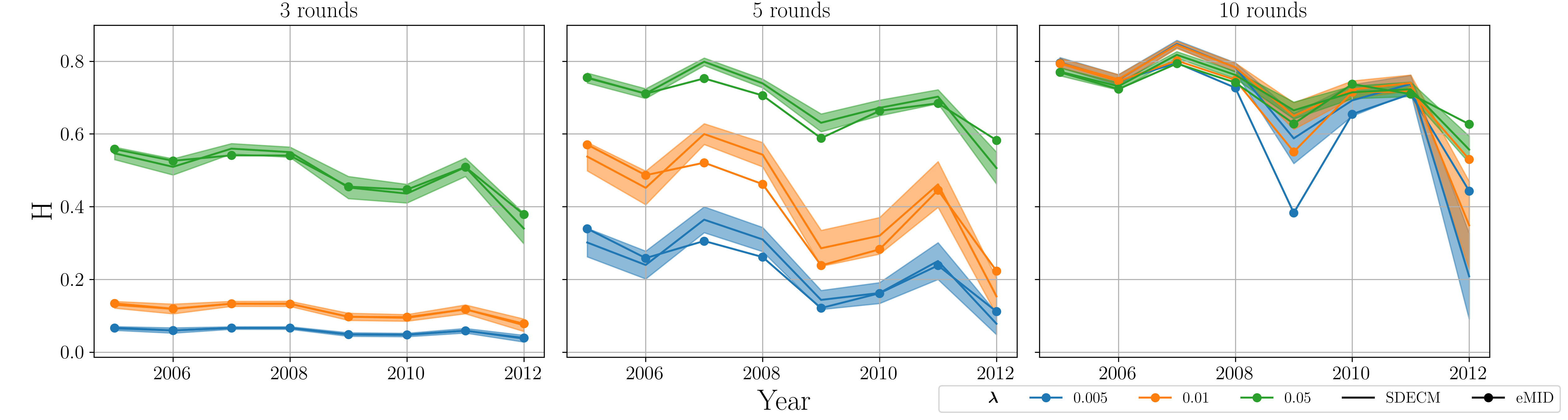
Figure 3: Linear DebtRank dynamics of eq. (6): aggregate systemic risk $H$ in the various yearly networks, for some sample iteration steps of the dynamics (3, 5 and 10 rounds in the left, middle and right panel respectively) and varying initial shock (0.5% in blue, 1% in orange and 5% in green). Values observed in the empirical networks are indicated with solid dots (connected with lines), whereas SDECM expected values are represented with lines and shaded areas (indicating ensemble mean and standard deviation).

We remark that we only use DebtRank valuation functions in this section due to the lack of initial defaults that could trigger Furfine dynamics. For the linear DebtRank of eq. (6), Figure 3 shows expected and observed aggregate systemic risk for some sample iteration steps of the algorithm. We firstly notice how the aggregate risk $H$ can be different in the various yearly networks considered. The contagion dynamic runs faster for initial shocks of larger magnitude, but the stationary values of $H$ are usually very close between each other. Concerning the relation between observed and expected systemic risk, we observe a good agreement during the early stages of the dynamics (the observed value of $H$ falls within the confidence region of one standard deviation $\sigma$ for the expected $H$). Slight deviations start to appear for intermediate iteration steps (particularly for 2007 and 2008), while at convergence we observe only two economically significant deviations: in the 2009 network, observed systemic risk is 14.8% (3.3$\sigma$) and 12.7% (3$\sigma$) lower than expected for $\lambda$ equal to 0.005 and 0.01, even if the deviation reduces only to 3% (0.8$\sigma$) for the higher value 0.05; the 2012 network has the opposite behaviour, with an observed $H$ that is 50%, 25%, and 13% (1.18, 1.27, and 1.94 $\sigma$) higher than expected, respectively for $\lambda$ equal to 0.005, 0.01 and 0.05.

A clearer picture of the contagion propagation can be obtained from Figure 4, where we plot for each yearly network how the value of $H$ grows with the iteration steps (i.e., the rounds of contagion). Table 1 in ”Appendix B. Results tables” provides numerical details about the Figure. The only yearly networks for which eMID is statistically different from the expected systemic risk for all the values of $\lambda$ are 2007, 2008, 2009 and 2012. We confirm that in 2007 and 2008, the observed systemic risk is slightly lower than expected, with an economically significant difference only during the first iterations of the algorithm. However, 2009 stands out for the magnitude of the deviation, especially for smaller initial shocks: observed systemic risk is on average 15.3% (2.54$\sigma$) lower than what is expected from the balance sheets distribution. In 2012 we observe an opposite behaviour with the e-MID network generating, on average, a relative equity loss that is 47.2% higher (1.28$\sigma$). All the negative deviations tend to disappear for large initial shocks ($\lambda=0.05$) but remain significant for the 2012 network, with observed systemic risk that is on average 12% (1.73$\sigma$) higher than expected.

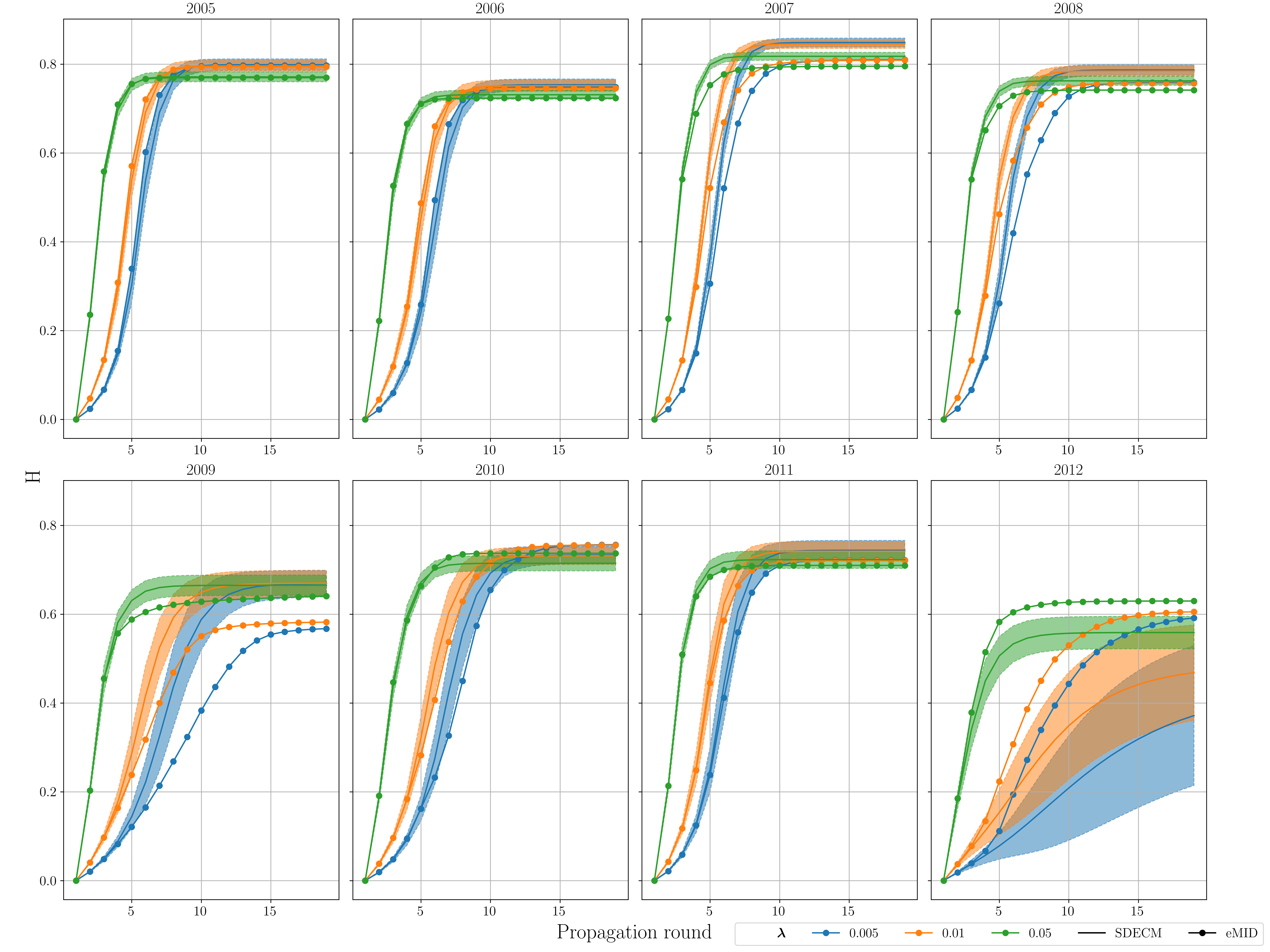
Figure 4: Linear DebtRank dynamics of eq. (6): evolution of aggregate systemic risk $H$ as a function of the iteration step, for the various yearly networks considered and varying initial shock $\lambda$. Observed and expected values are indicated respectively with solid dots (connected by lines) and line plus shaded area (indicating ensemble mean and standard deviation).

For the case of nonlinear DebtRank, Figure 5 further shows the stationary value of the average relative equity loss as a function of the claims re-evaluation factor $\alpha$. Table 2 contains the related numerical details. The statistical significance of the analysis shows large variations depending on the model parameters, with some significant deviations for all years. However, the bulk of those deviations is consistent with the previous analysis: 2007, 2008, 2009 and 2012 mean relative loss difference is statistically significant with the same sign for all the values of the shock $\lambda\leq 0.25$, with the latter two yearly networks being economically significant. However, for the largest shock (0.35) the results are not so sharply defined, with also the 2008 and 2009 networks showing positive statistically significant deviations, albeit very small in magnitude. Only 2012 remains consistent with the other values of the shock parameter with large and significant positive deviations.

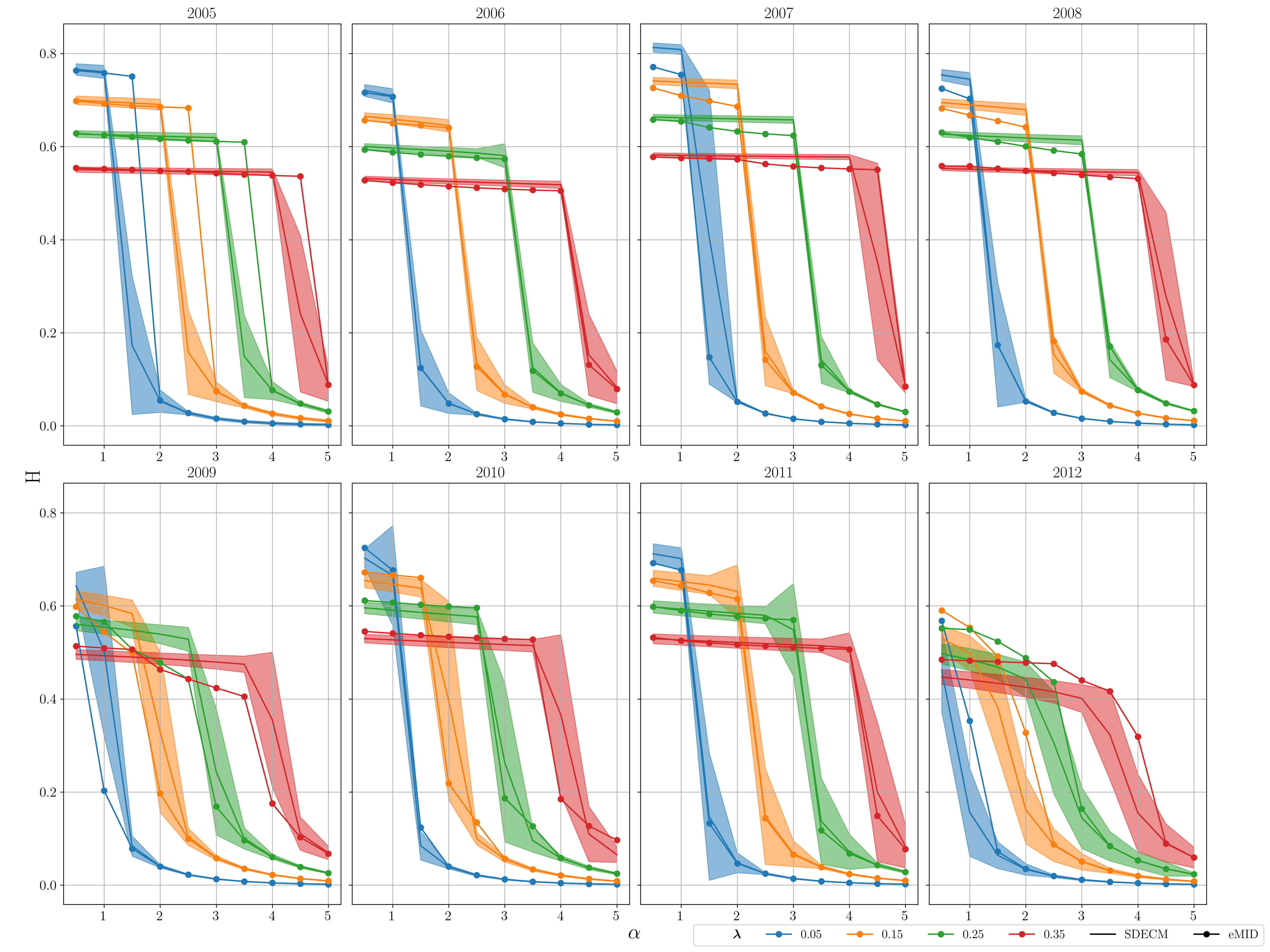
Figure 5: Nonlinear DebtRank dynamics of eq. (7): stationary level of aggregate systemic risk $H$ as a function of the nonlinearity parameter $\alpha$, for the various yearly networks considered and varying initial shock $\lambda$. Observed and expected values are indicated respectively with solid dots (connected by lines) and line plus shaded area (indicating ensemble mean and standard deviation). We recall that $\alpha=0$ corresponds to linear DebtRank, while $\alpha\to\infty$ leads in principle to contagion on default.

3.2 Systemic relevance

In this section, we analyse the systemic relevance of each bank by using two indicators, the impact $I_{i}$ and the vulnerability $V_{i}$ (Cimini and Serri,, 2016). The impact $I_{i}$ measures the relative amount of equity lost by the system as a consequence of the default of bank $i$

$$I_{i}=1-\frac{\sum_{j\neq i}^{n}E_{j}(t^{*}|E_{i}(1)=0))}{\sum_{j\neq i}^{n}E_{j}(0)}$$ (9)

while the vulnerability $V_{i}$ assesses the average equity loss of bank $i$ due to the default of another bank in the network

$$V_{i}=\frac{1}{n-1}\sum_{j\neq i}^{n}\left[1-\frac{E_{i}(t^{*}|E_{j}(1)=0)}{E_{i}(0)}\right]$$ (10)

In both cases, the condition $t^{*}|E_{i}(1)=0$ indicates the final step of a dynamics with initial condition given by the default of bank $i$ and no shocks to all other banks.

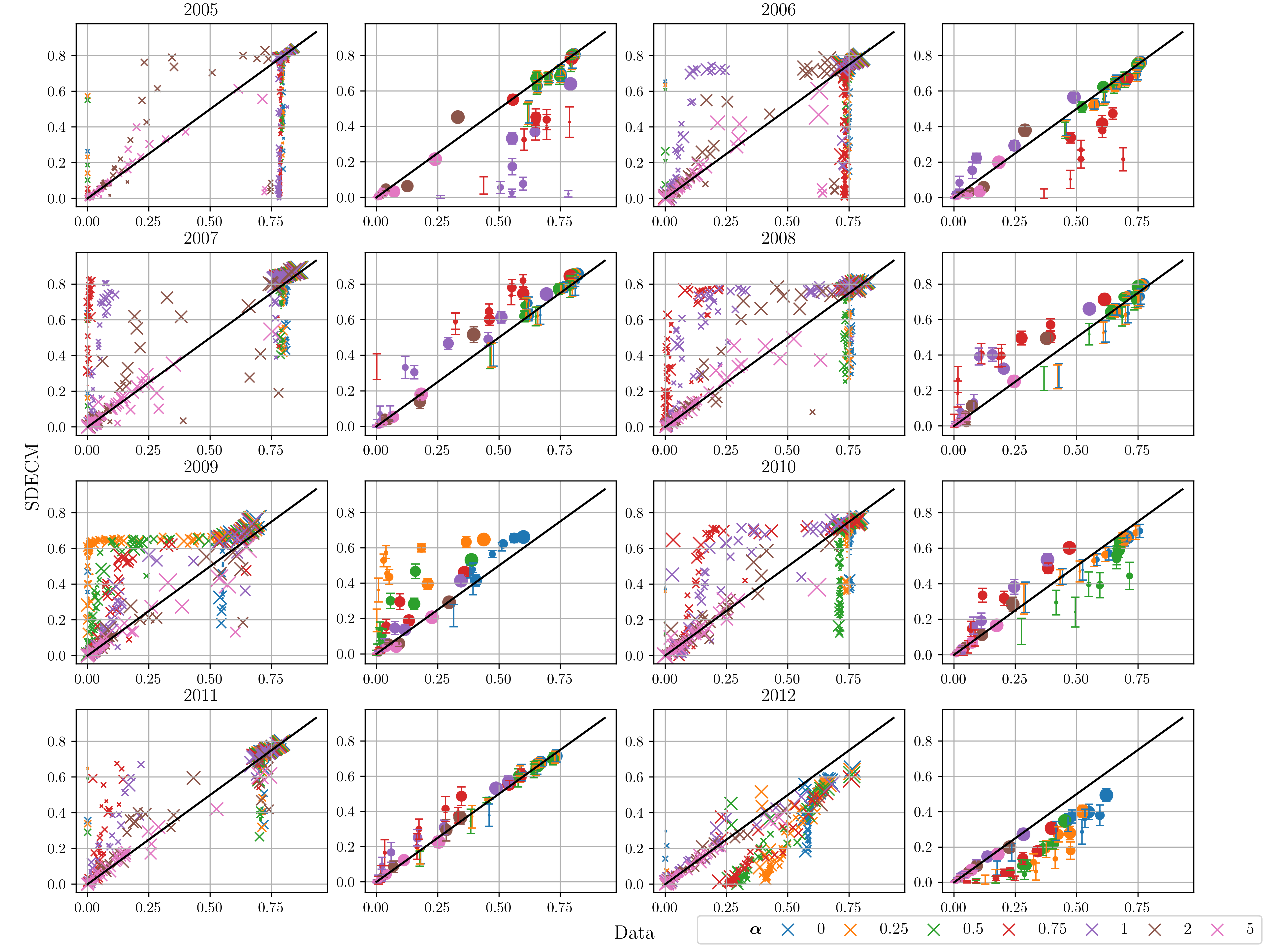
Figure 6: Scatter plot of observed (Data) and expected (SDECM) impact of individual banks in the system for the various yearly networks considered. Different values of the nonlinearity parameter $\alpha$ are displayed with varying colours. For each year, the plot on the left shows each bank with a different point, while the plot on the right show the average value of impact in the equity decile group.

Figures 6 and 7 show the impact and vulnerability of each bank in the various yearly networks. First, we note that when considering individual banks, sensible deviations (both negative and positive) are present, especially when the nonlinearity of the valuation function is low – that is, when banks’ probabilities of default increase as soon as their equity starts decreasing. This suggests that the position of a bank in the network matters, especially when even small losses impact the default probability and thus the value of exposures. Figure 8 confirms this observation: when the Furfine valuation function is used, deviations are nearly non-existent in all years.

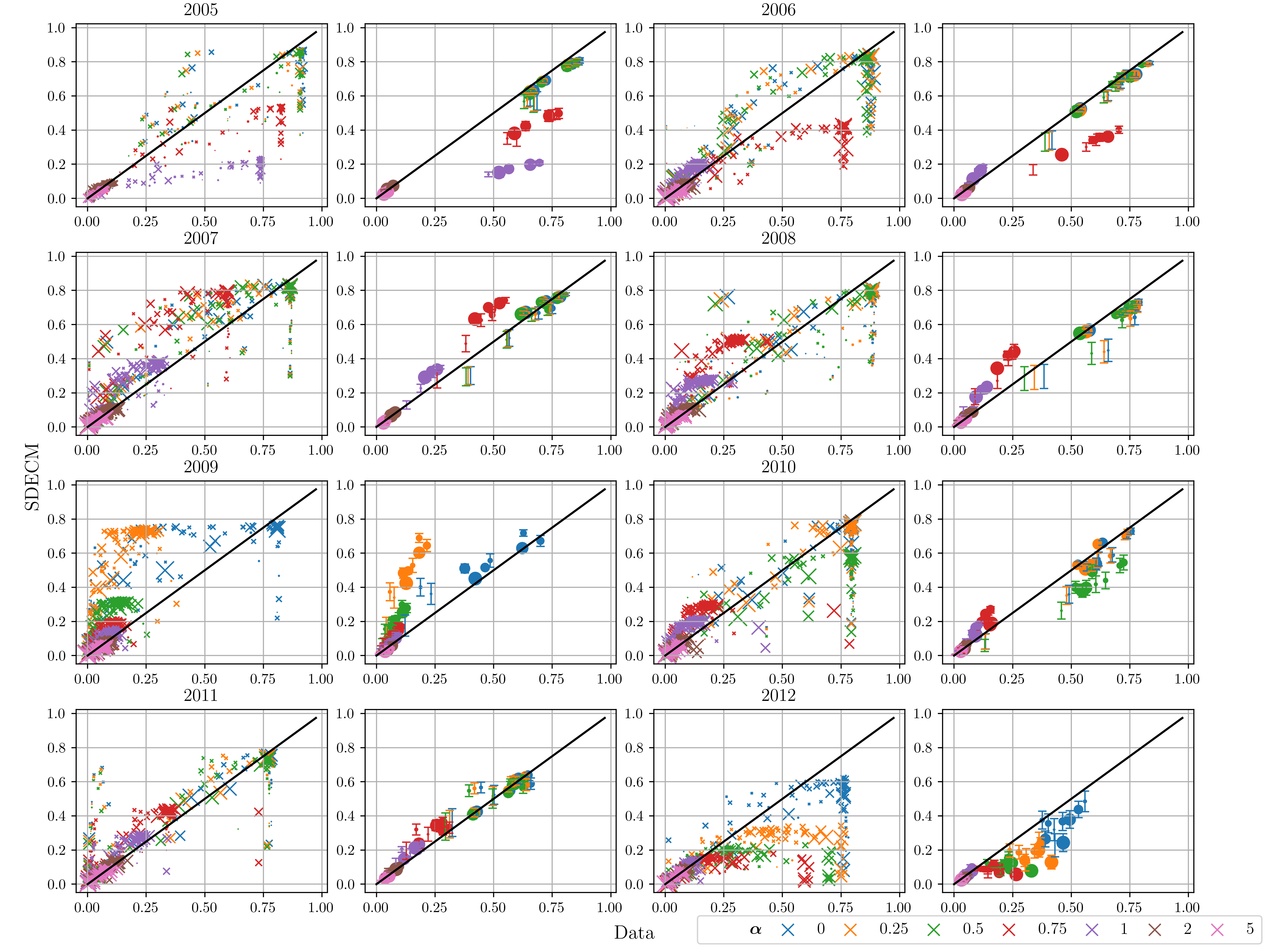
Figure 7: Scatter plot of observed (Data) and expected (SDECM) vulnerability of individual banks in the system, for the various yearly networks considered. Different values of the nonlinearity parameter $\alpha$ are displayed with varying colours. For each year, the plot on the left shows each bank with a different point, while the plot on the right show the average value of vulnerability in the equity decile group.

Second, averaging banks in equity classes reduces the magnitude of the deviations, confirming the result of the previous section that the aggregate level of systemic risk can be inferred from balance sheet structures. Again, this last observation is valid only for the years in which there are no extreme market disruptions. Even after averaging banks in equity classes, in 2009 deviations from the null model are clustered above the diagonal line where expected and observed systemic relevance are equal, indicating that banks are less risky than what their balance sheet would imply. In 2012 deviations are instead positive.

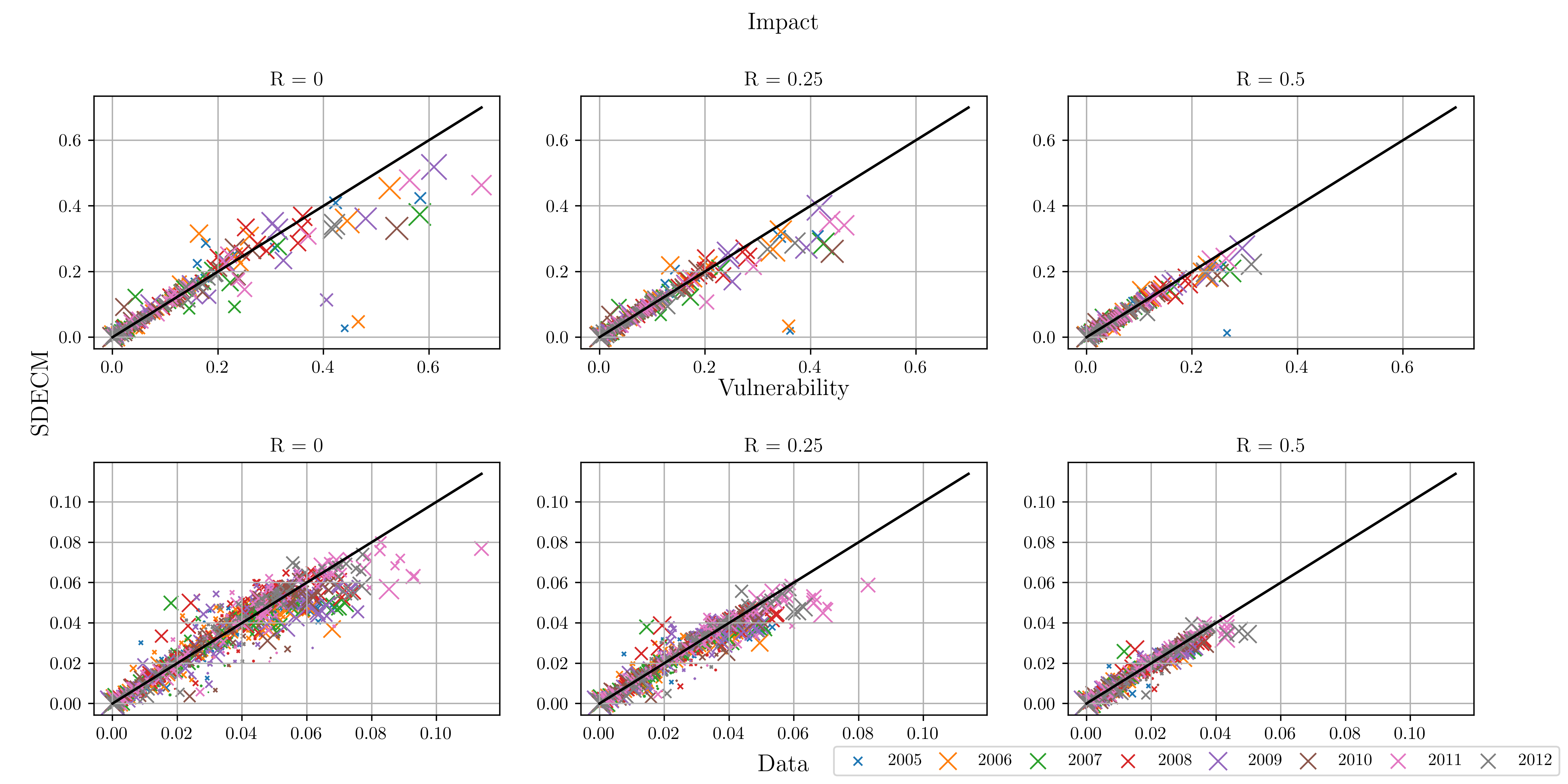
Figure 8: Scatter plot of observed (Data) and expected (SDECM) impact of individual banks in the system, for the Furfine dynamics of eq. (5) with different recovery rates $R$. Different colors denote values related to each yearly network.

3.3 Discussion

We argue that the most significant deviations we observed are due to two very disruptive events for the interbank market, namely the default of Lehman Brothers in September 2008 and the introduction of the 3-year Longer-Term Refinancing Operations (LTRO) by the ECB.

This observation is supported by the results of Affinito and Pozzolo, (2017). Using supervisory data from the Bank of Italy, they showed that those two events changed the network structure of the Italian interbank market. They found that the collapse of Lehman Brothers reduced the connectivity of the interbank network while, in some specifications of the model, the liquidity crisis of August 2007 is statistically insignificant. On the contrary, the announcement of the 3-year LTRO by the ECB had the opposite effect. The operations shifted the distribution of the centralities towards the most connected banks and thus to “smoother liquidity circulation among banks”. With another methodology, Barucca and Lillo, (2018) confirmed the impact of the 3-year LTRO on e-MID. They analysed the network structure of the market from 2010 to 2014 and showed that the 3-year LTRO had a profound impact on the banks’ trading behaviour and thus on the network configuration. Historical lenders exited the market, and borrowing banks and new institutions stepped in taking their place, sensibly changing the network structure.

The different signs of the deviations caused by the two events can be explained by the different consequences that they had on banks’ behaviour. Angelini et al., (2011) showed that after the liquidity crisis of August 2007, interest rates started to reflect the creditworthiness of the borrowing counterparty. Unfortunately, their analysis stops at December 2008 and thus does not help explain the results presented in this paper. However, Afonso et al., (2011), through an analysis of the overnight Federal Funds market, found that the default of Lehman Brothers increased concerns in the market for counterparty risk, reducing liquidity and increasing costs for weaker banks. The larger impact of Lehman’s default is consistent with Affinito and Pozzolo, (2017) and with the deviations from the expected systemic risk that we detect in our analysis. The negative deviations that we observe in the 2009 panels of Figures 6 and 7 suggest that banks have been able to reduce not only their direct counterparty risk but also to internalise part of the externalities that are generated in a network setting. Another non-trivial result is that this behaviour emerges at the aggregate level, as shown in Figures 4 and 5, with lower observed systemic risk.

On the contrary, the introduction of the 3-year LTROs could have impacted the interbank market consistently with the risk-taking channel of monetary policy (Borio and Zhu,, 2008). Our results suggest that the central bank’s provision of very long-term liquidity has affected the interbank market, possibly by increasing banks’ willingness to take on risk and by reducing the perceived risk of contagion. The reaction of the banking system has thus generated an increased systemic risk, both at the individual (2012 panels of Figures 6-7) and at the aggregate level (Figures 4-5).

Notice how these results are consistent with the network formation mechanism that the null model implies. In the SDECM, the probability of a connection between two banks is proportional to the number of counterparties and total interbank assets and liabilities. Therefore the model describes a matching process in which individual institutions choose their counterparties independently from their probability of default. The evidence from Angelini et al., (2011) and Afonso et al., (2011) suggests that counterparty risk became more relevant after the disruptions in the interbank market, making the SDECM unable to capture the systemic risk observed in the network. On the contrary, the introduction of the 3-year LTRO could have heterogeneously reduced risk aversion, thereby introducing additional features in the matching mechanism of the market and generating more systemic risk than what would be expected given the balance sheet composition of the system. It must be noted that those conclusions are nowhere rigorous and that further research is needed to uncover the effect of those events in the network formation process.

Moreover, the results highlight the importance of considering the exact network structure when the model used for the evaluation entails distress contagion dynamics: when the nonlinearity of DebtRank ($\alpha$) is high and with the Furfine valuation function, the deviations disappear. This suggests that, when the model approaches contagion at default, the exact network structure is less relevant. These results corroborate the analysis of Glasserman and Young, (2015), who find that network feedback with the Eisenberg-Noe model increase contagion only by 1.75%. On the contrary, distress contagion enhances the importance of the feedback effects on the network structure, as shown by the large deviations in some yearly networks.

4 Conclusion

In this paper, we contribute to the growing literature about the effects of the network structure on systemic risk, by introducing the notion of expected systemic risk, i.e. the level of systemic risk that is due to the market’s balance sheets but not to a specific network configuration. This quantity is obtained by using an appropriate maximum entropy network model constraining relevant balance sheet variables. We compute observed and expected systemic risk, using the Network Asset Valuation framework (Barucca et al.,, 2020), in a dataset of interbank exposures from the e-MID market, augmented with equity information from BankFocus data.

The results show that aggregate systemic risk, measured through linear and nonlinear DebtRank, is usually well explained by the distribution of balance sheets. However, significant deviations are present in the 2009 and 2012 networks. Conversely, the indexes of systemic relevance for individual banks present sizeable differences with clusters of banks that show both positive and negative deviations for DebtRank, while the results from the Furfine algorithm are more consistent with the null model. This suggests that some banks are riskier than what is implied by their balance sheet because of their position in the network. The lower is the shock absorption capacity of banks (i.e., the faster the probability of default increases with equity losses), the stronger is the effect of the position in the network. In the limiting case of contagion on default, nearly all the deviations disappear. Moreover, averaging banks’ systemic relevance in equity deciles decreases the magnitude of the deviations, except for 2009 and 2012.

The negative deviations present for aggregate and individual systemic risk in 2009 could signal that, after the default of Lehman Brothers in September 2009, banks collectively started to minimise their counterparty risk in response to the increased concerns about possible bankruptcies. While this could be an obvious result at the individual level, the emergence of a reduction of aggregate systemic risk in a network context is not trivial. The result points towards the existence of an endogenous mechanism that allows banks to reduce their risk of being affected by contagion while also reducing systemic risk for the entire system. The same reasoning can be applied to the 2012 network, with the 3-year LTRO increasing banks’ willingness to take on risk, reducing the perceived counterparty risk, and thus increasing the scope of contagion. While the model does not allow us to draw a causal relationship between the observed deviations and the two crisis events, we note that these observations are in line with the existing literature on interbank markets.

Furthermore, our results corroborate the existing literature on interbank contagion: the network structure matters, particularly during systemic events. Those observations demonstrate that it essential to include networks in stress testing models and collect data to measure the scope of contagion accurately. However, further research is needed to prove an exact causal relation among those events and systemic risk and to uncover the network formation processes that generate the observed effects. A deeper understanding of those mechanisms would be valuable for designing incentive policies that are able to reduce the instability of the network with minimal effects on banks’ interbank lending and funding choices.

Appendix A. Separable Directed Enhanced Configuration Model

In this appendix we describe the formal steps that define the Separable Directed Enhanced Configuration Model (SDECM). We remand the reader to Gabrielli et al., (2019) for an extended discussion (about the case of undirected networks) and to Cimini et al., (2019) for a general introduction to maximum entropy models of networks.

We start by considering a directed weighted network of $n$ nodes, denoting by ${\cal V}$ the set of all ordered node pairs so that $|{\cal V}|=n(n-1)$. The network is univocally defined through a configuration ${\cal C}=(G,A)$ composed by: the binary adjacency matrix $G=\{g_{ij}\}_{(i,j)\in{\cal V}}$ that defines the set of existing links $(i,j)\in{\cal L}\subseteq{\cal V}$ (i.e., the set of node pairs with $a_{ij}=1$), and the weighted adjacency matrix $A=\{A_{ij}\}_{(i,j)\in{\cal V}}$ that defines the set of weights $\{A_{ij}\}_{(i,j)\in{\cal L}}$ associated to them. Our goal is to construct an ensemble $\Omega$ of such networks that are maximally random, except for some properties that are constrained on average. The probability distribution $P({\cal C})$, that is, the occurrence probability of configuration ${\cal C}$ within the ensemble $\Omega$, is obtained by maximising the Shannon entropy $S=-\sum_{{\cal C}\in\Omega}P(\cal C)\log P(\cal C)$ subject to the normalisation condition plus the set of constraints that we want to impose.

In our case we have four constraints for each node $i$: the out-degree $k_{i}^{out}=\sum_{j\in\cal V}g_{ij}$ and in-degree $k_{i}^{in}=\sum_{j\in\cal V}g_{ji}$ plus the out-strength $s_{i}^{out}=\sum_{j\in\cal L}A_{ij}$ and in-strength $s_{i}^{in}=\sum_{j\in\cal L}A_{ji}$. In principle these constraints can be imposed simultaneously; however we use a two-step entropy maximisation procedure that leads to an easier numerical implementation:

1. We first constrain the average in/out-degrees only, obtaining the probability of the binary configuration $A$:

   $$\pi(G)=\prod_{(i,j)\in{\cal V}}\frac{e^{-(\alpha^{out}_{i}+\alpha^{in}_{j})g_{ij}}}{1+e^{-(\alpha^{out}_{i}+\alpha^{in}_{j})}}$$ (11)

   where $\alpha_{i}^{out}$ and $\alpha_{i}^{in}$ are the Lagrange multipliers associated to the out/in-degree of node $i$.

2. Then, for each $G$, we constrain the average in/out-strengths, obtaining the probability density of the link weights conditional to $G$

   $$q(W_{{\cal L}})=\prod_{(i,j)\in{\cal L}}(\beta_{i}^{out}+\beta_{j}^{in})e^{-(\beta_{i}^{out}+\beta_{j}^{in})A_{ij}}$$ (12)

   where $\beta_{i}^{out}$ and $\beta_{i}^{in}$ are the Lagrange multipliers associated to the out/in-strength of node $i$.

Overall the SDECM is defined by the joint probability distribution $P(G,A)=\pi(G)q(A_{{\cal L}})$. Finally to obtain a model for a specific empirical network configuration ${\cal C}^{*}$ we maximise the likelihood of ${\cal C}^{*}$ in the ensemble. This corresponds to finding the values of the Lagrange multipliers that satisfy, $\forall i$:

$$\begin{cases}[k_{i}^{out}]^{*}=\sum_{j:(i,j)\in{\cal V}}\dfrac{1}{1+e^{(\alpha^{out}_{i}+\alpha^{in}_{j})}}\\ [k_{i}^{in}]^{*}=\sum_{j:(i,j)\in{\cal V}}\dfrac{1}{1+e^{(\alpha^{in}_{i}+\alpha^{out}_{j})}}\\ [s_{i}^{out}]^{*}=\sum_{j:(i,j)\in{\cal L}}\dfrac{(\beta_{i}^{out}+\beta_{j}^{in})^{-1}}{1+e^{(\alpha^{out}_{i}+\alpha^{in}_{j})}}\\ [s_{i}^{in}]^{*}=\sum_{j:(i,j)\in{\cal L}}\dfrac{(\beta_{i}^{in}+\beta_{j}^{out})^{-1}}{1+e^{(\alpha^{in}_{i}+\alpha^{out}_{j})}}\end{cases}$$ (13)

where $[k_{i}^{out}]^{*}$, $[k_{i}^{in}]^{*}$, $[s_{i}^{out}]^{*}$, $[s_{i}^{in}]^{*}$ are the numerical values that constraints assume on the empirical network ${\cal C}^{*}$.

Appendix B. Results tables

	Year	2005	2006	2007	2008	2009	2010	2011	2012
$\bm{\lambda}$	$\bm{t}$
0.005	3	$0.026$ 0.328 (69.3)	$-0.001$ -0.005 (61.1)	$0.001$ 0.023 (53.3)	$-0.002$ -0.043 (51.4)	$-0.002$ -0.019 (57.2)	$0.017$ 0.165 (64.0)	$-0.004$ -0.039 (53.1)	$0.049$ 0.2 (72.4)
	5	$0.126$ 0.971 (85.1)	$0.079$ 0.496 (76.6)	$-0.161^{**}$ -1.649 (3.8)	$-0.156^{*}$ -1.459 (5.1)	$-0.157$ -0.861 (17.7)	$-0.004$ -0.024 (55.0)	$-0.049$ -0.242 (44.3)	$0.43$ 1.124 (89.8)
	10	$-0.001$ -0.085 (44.4)	$-0.005$ -0.262 (37.9)	$-0.061^{***}$ -5.1 (0.0)	$-0.071^{***}$ -4.324 (0.0)	$-0.349^{***}$ -2.967 (0.7)	$-0.055$ -0.877 (16.3)	$-0.038$ -1.15 (11.3)	$1.126^{*}$ 1.991 (93.7)
	20	$-0.002$ -0.131 (42.6)	$-0.007$ -0.4 (32.4)	$-0.046^{***}$ -3.894 (0.0)	$-0.036^{**}$ -2.379 (1.7)	$-0.151^{***}$ -3.379 (0.1)	$0.032$ 1.173 (87.9)	$-0.03$ -0.999 (17.3)	$0.558^{*}$ 1.357 (92.0)
	Convergence	$-0.002$ -0.131 (42.6)	$-0.007$ -0.4 (32.4)	$-0.045^{***}$ -3.879 (0.0)	$-0.036^{**}$ -2.379 (1.7)	$-0.148^{***}$ -3.34 (0.1)	$0.032$ 1.177 (88.1)	$-0.03$ -0.999 (17.3)	$0.403^{*}$ 1.176 (92.3)
0.010	3	$0.028$ 0.388 (69.3)	$0.003$ 0.028 (61.1)	$0.001$ 0.023 (53.3)	$-0.002$ -0.04 (51.4)	$-0.002$ -0.017 (57.2)	$0.019$ 0.199 (64.1)	$-0.003$ -0.033 (53.1)	$0.053$ 0.23 (72.4)
	5	$0.061$ 0.84 (80.4)	$0.077$ 0.752 (78.8)	$-0.131^{***}$ -2.754 (0.6)	$-0.149^{**}$ -2.427 (1.2)	$-0.165$ -0.956 (15.4)	$-0.117$ -0.744 (23.2)	$-0.034$ -0.253 (38.9)	$0.456^{*}$ 1.38 (91.6)
	10	$-0.002$ -0.127 (42.9)	$-0.007$ -0.403 (32.3)	$-0.051^{***}$ -4.384 (0.0)	$-0.044^{***}$ -2.919 (0.4)	$-0.152^{***}$ -2.696 (0.7)	$-0.011$ -0.321 (34.2)	$-0.032$ -1.057 (14.6)	$0.52$ 1.504 (89.7)
	20	$-0.002$ -0.13 (42.8)	$-0.007$ -0.44 (31.0)	$-0.043^{***}$ -3.707 (0.0)	$-0.035^{**}$ -2.368 (1.7)	$-0.13^{***}$ -3.063 (0.1)	$0.033$ 1.231 (89.8)	$-0.029$ -0.967 (18.2)	$0.284^{*}$ 1.271 (93.0)
	Convergence	$-0.002$ -0.13 (42.8)	$-0.007$ -0.44 (31.0)	$-0.043^{***}$ -3.696 (0.0)	$-0.035^{**}$ -2.368 (1.7)	$-0.127^{***}$ -2.997 (0.2)	$0.033$ 1.232 (89.8)	$-0.029$ -0.967 (18.2)	$0.25^{*}$ 1.264 (93.1)
0.050	3	$0.021$ 0.672 (74.8)	$0.033$ 0.75 (78.6)	$-0.033^{*}$ -1.307 (8.7)	$-0.017$ -0.66 (24.5)	$0.005$ 0.077 (56.6)	$0.025$ 0.427 (68.1)	$0.001$ 0.018 (49.0)	$0.113$ 0.919 (82.9)
	5	$0.001$ 0.081 (51.5)	$-0.001$ -0.03 (45.2)	$-0.057^{***}$ -4.434 (0.0)	$-0.045^{***}$ -2.787 (0.4)	$-0.067^{**}$ -1.732 (3.5)	$-0.012$ -0.385 (34.7)	$-0.026$ 30-0.942 (17.6)	$0.152^{**}$ 1.753 (95.3)
	10	$-0.002$ -0.163 (41.5)	$-0.011$ -0.762 (20.5)	$-0.029^{***}$ -2.676 (0.5)	$-0.028^{**}$ -2.094 (2.6)	$-0.055^{*}$ -1.585 (6.0)	$0.032^{*}$ 1.311 (90.4)	$-0.018$ -0.666 (28.0)	$0.125^{**}$ 1.89 (96.4)
	20	$-0.002$ -0.163 (41.5)	$-0.011$ -0.763 (20.5)	$-0.027^{***}$ -2.476 (0.8)	$-0.027^{**}$ -2.073 (2.6)	$-0.036$ -1.028 (15.4)	$0.032^{*}$ 1.311 (90.4)	$-0.018$ -0.654 (28.0)	$0.127^{**}$ 1.936 (96.6)
	Convergence	$-0.002$ -0.163 (41.5)	$-0.011$ -0.763 (20.5)	$-0.027^{***}$ -2.473 (0.8)	$-0.027^{**}$ -2.073 (2.6)	$-0.029$ -0.844 (19.6)	$0.032^{*}$ 1.311 (90.4)	$-0.018$ -0.654 (28.0)	$0.127^{**}$ 1.936 (96.6)

Table 1: Linear DebtRank. This table reports data about the relative equity loss of the system $H$ with the linear DebtRank valuation function, depicted in Figure 4. Each row corresponds to a combination of the initial shock $\lambda$ and contagion round $t$ while the columns correspond to the yearly networks. The top element from each cell corresponds to the relative deviation of $H$ obtained with the eMID network from its average in the SDECM; the middle elements in italics correspond to the difference between eMID and the configuration model average divided by the SDECM standard deviation; the bottom element in parenthesis reports the percentile position of eMID with respect to the distribution of $H$ generated by the SDECM. *, ** and *** denote the significance of the deviation and highlight if eMID’s $H$ is either in the top or bottom 10%, 5% or 1% of the distribution generated by the SDECM.

	Year	2005	2006	2007	2008	2009	2010	2011	2012
$\bm{\lambda}$	$\bm{\alpha}$
0.05	0.5	$-0.003$ -0.189 (40.1)	$-0.007$ -0.374 (33.2)	$-0.051^{***}$ -4.264 (0.0)	$-0.039^{**}$ -2.465 (1.4)	$-0.135^{***}$ -2.978 (0.2)	$0.032$ 1.12 (86.2)	$-0.028$ -0.915 (21.1)	$0.231$ 1.197 (88.9)
	1.0	$-0.003$ -0.184 (41.1)	$-0.003$ -0.133 (45.0)	$-0.067^{***}$ -5.079 (0.0)	$-0.057^{***}$ -2.93 (0.4)	$-0.596^{*}$ -1.644 (7.3)	$0.017$ 0.106 (31.3)	$-0.035$ -1.065 (15.2)	$1.256^{*}$ 2.082 (94.9)
	1.5	$3.352^{**}$ 3.909 (95.3)	$-0.002$ -0.003 (78.8)	$-0.636$ -0.817 (20.6)	$0.0$ 0.0 (86.9)	$-0.063$ -0.246 (33.1)	$0.462^{**}$ 1.276 (98.5)	$-0.099$ -0.107 (79.4)	$0.121$ 0.273 (83.3)
	2.5	$0.018$ 0.138 (70.4)	$-0.001$ -0.012 (58.7)	$-0.008$ -0.186 (45.3)	$-0.01$ -0.224 (43.8)	$-0.007$ -0.099 (49.6)	$0.008$ 0.078 (63.0)	$-0.007$ -0.081 (51.0)	$0.027$ 0.177 (66.5)
	5.0	$-0.045$ -0.039 (67.8)	$-0.001$ -0.016 (57.7)	$0.001$ 0.034 (52.8)	$-0.003$ -0.068 (49.9)	$-0.001$ -0.013 (51.8)	$0.003$ 0.03 (61.7)	$-0.004$ -0.048 (52.0)	$0.019$ 0.154 (62.8)
0.15	0.5	$-0.002$ -0.187 (39.2)	$-0.013$ -1.066 (13.7)	$-0.02^{**}$ -1.995 (2.9)	$-0.018^{*}$ -1.462 (7.8)	$-0.025$ -0.831 (20.5)	$0.027$ 1.179 (87.5)	$-0.008$ -0.321 (38.7)	$0.114^{**}$ 2.131 (97.8)
	1.0	$-0.006$ -0.454 (31.0)	$-0.014$ -0.947 (16.0)	$-0.04^{***}$ -3.602 (0.0)	$-0.032^{**}$ -2.332 (2.2)	$-0.094^{***}$ -2.525 (0.1)	$0.031$ 1.199 (88.5)	$-0.014$ -0.476 (33.2)	$0.109^{*}$ 1.48 (91.9)
	1.5	$-0.008$ -0.511 (27.9)	$-0.01$ -0.587 (27.2)	$-0.052^{***}$ -4.379 (0.0)	$-0.043^{***}$ -2.729 (0.8)	$-0.146^{***}$ -2.925 (0.5)	$0.035$ 1.202 (88.6)	$-0.026$ -0.838 (23.5)	$0.287$ 1.075 (83.2)
	2.5	$3.312^{**}$ 5.786 (97.9)	$-0.046$ -0.106 (58.8)	$-0.115$ -0.25 (26.4)	$0.19^{**}$ 0.729 (96.8)	$-0.04$ -0.224 (40.0)	$0.354^{**}$ 2.596 (98.5)	$-0.026$ -0.037 (83.4)	$0.016$ 0.04 (71.7)
	5.0	$0.005$ 0.021 (68.0)	$-0.001$ -0.018 (57.8)	$0.001$ 0.022 (52.4)	$-0.003$ -0.076 (49.4)	$-0.001$ -0.02 (51.6)	$0.003$ 0.034 (61.6)	$-0.004$ -0.051 (52.1)	$0.019$ 0.155 (63.2)
0.25	0.5	$0.002$ 0.178 (53.0)	$-0.011$ -1.095 (12.6)	$-0.008$ -0.94 (18.1)	$0.005$ 0.535 (68.8)	$0.031$ 1.314 (88.9)	$0.026^{*}$ 1.283 (90.2)	$0.0$ 0.016 (50.9)	$0.11^{***}$ 2.54 (99.5)
	1.0	$-0.001$ -0.07 (45.0)	$-0.016^{*}$ -1.408 (7.9)	$-0.012$ -1.333 (10.1)	$-0.007$ -0.633 (25.9)	$0.02$ 0.763 (78.5)	$0.028$ 1.241 (88.6)	$-0.006$ -0.23 (41.8)	$0.133^{***}$ 2.703 (99.6)
	1.5	$-0.005$ -0.393 (32.8)	$-0.018^{*}$ -1.488 (7.3)	$-0.03^{***}$ -3.118 (0.2)	$-0.017^{*}$ -1.431 (8.5)	$-0.075^{***}$ -2.418 (0.5)	$0.028$ 1.168 (87.5)	$-0.01$ -0.386 (35.9)	$0.117^{**}$ 2.012 (97.2)
	2.5	$-0.012$ -0.844 (19.3)	$-0.018$ -1.101 (13.3)	$-0.047^{***}$ -4.508 (0.0)	$-0.04^{***}$ -2.767 (0.9)	$-0.162^{***}$ -3.334 (0.5)	$0.033$ 1.148 (87.8)	$-0.012$ -0.387 (35.7)	$0.426$ 1.187 (81.7)
	5.0	$0.014$ 0.131 (68.0)	$-0.002$ -0.029 (58.1)	$-0.002$ -0.041 (50.6)	$-0.005$ -0.123 (47.3)	$-0.004$ -0.058 (50.5)	$0.005$ 0.049 (61.2)	$-0.006$ -0.072 (51.3)	$0.019$ 0.126 (64.1)
0.35	0.5	$0.006$ 0.617 (68.4)	$-0.008$ -0.777 (22.0)	$-0.007$ -0.94 (18.4)	$0.01^{*}$ 1.275 (90.2)	$0.036^{*}$ 1.707 (92.6)	$0.029^{**}$ 1.656 (96.0)	$0.005$ 0.265 (59.1)	$0.084$ 2.293 (99.0)
	1.0	$0.004$ 0.418 (61.1)	$-0.013$ -1.266 (10.3)	$-0.01$ -1.187 (12.7)	$0.012^{*}$ 1.393 (92.5)	$0.034^{*}$ 1.524 (90.8)	$0.026^{*}$ 1.398 (93.2)	$-0.003$ -0.131 (45.1)	$0.094^{***}$ 2.357 (99.3)
	1.5	$0.003$ 0.252 (54.9)	$-0.017^{*}$ -1.575 (6.0)	$-0.011^{*}$ -1.337 (10.0)	$0.005$ 0.59 (72.4)	$0.033$ 1.42 (89.4)	$0.024$ 1.214 (89.9)	$-0.007$ -0.301 (38.2)	$0.107^{***}$ 2.419 (99.4)
	2.5	$-0.002$ -0.211 (39.1)	$-0.023^{**}$ -1.948 (3.7)	$-0.028^{***}$ -3.198 (0.2)	$-0.007$ -0.72 (22.5)	$-0.083^{***}$ -3.044 (0.1)	$0.023$ 1.011 (83.6)	$-0.009$ -0.377 (36.2)	$0.145^{***}$ 2.504 (99.5)
	5.0	$-0.011$ -0.027 (69.1)	$-0.042$ -0.1 (55.9)	$-0.027$ -0.146 (38.2)	$-0.02$ -0.341 (39.5)	$-0.026$ -0.127 (44.2)	$0.479^{***}$ 1.908 (99.3)	$-0.072$ -0.13 (49.3)	$-0.002$ -0.006 (66.7)

Table 2: Nonlinear DebtRank. This table reports data about the relative equity loss of the system $H$ with the nonlinear DebtRank valuation function, depicted in Figure 5. Each row corresponds to a combination of the initial shock $\lambda$ and nonlinearity parameter $\alpha$ while the columns correspond to the yearly networks. The top element from each cell corresponds to the relative deviation of $H$ obtained with the eMID network from its average in the SDECM; the middle elements in italics correspond to the difference between eMID and the configuration model average divided by the SDECM standard deviation; the bottom element in parenthesis reports the percentile position of eMID with respect to the distribution of $H$ generated by the SDECM. *, ** and *** denote the significance of the deviation and highlight if eMID’s $H$ is either in the top or bottom 10%, 5% or 1% of the distribution generated by the SDECM.

References

- Acemoglu et al., (2015) Acemoglu, D., Ozdaglar, A., and Tahbaz-Salehi, A. (2015). Systemic risk and stability in financial networks. American Economic Review, 105(2):564–608.
- Affinito and Pozzolo, (2017) Affinito, M. and Pozzolo, A. F. (2017). The interbank network across the global financial crisis: Evidence from Italy. Journal of Banking and Finance, 80:90–107.
- Afonso et al., (2011) Afonso, G., Kovner, A., and Schoar, A. (2011). Stressed, not frozen: The federal funds market in the financial crisis. Journal of Finance, 66(4):1109–1139.
- Allen and Gale, (2000) Allen, F. and Gale, D. (2000). Financial contagion. Journal of Political Economy, 108(1):1–33.
- Angelini et al., (2011) Angelini, P., Nobili, A., and Picillo, C. (2011). The Interbank Market after August 2007: What Has Changed, and Why? Journal of Money, Credit and Banking, 43(5):923–958.
- Bardoscia et al., (2021) Bardoscia, M., Barucca, P., Battiston, S., Caccioli, F., Cimini, G., Garlaschelli, D., Saracco, F., Squartini, T., and Caldarelli, G. (2021). The physics of financial networks. Nature Reviews Physics, 3(7):490–507.
- Bardoscia et al., (2015) Bardoscia, M., Battiston, S., Caccioli, F., and Caldarelli, G. (2015). DebtRank: A microscopic foundation for shock propagation. PLoS ONE, 10(6):1–13.
- Bardoscia et al., (2017) Bardoscia, M., Battiston, S., Caccioli, F., and Caldarelli, G. (2017). Pathways towards instability in financial networks. Nature Communications, 8.
- Bardoscia et al., (2016) Bardoscia, M., Caccioli, F., Perotti, J. I., Vivaldo, G., and Caldarelli, G. (2016). Distress propagation in complex networks: The case of non-linear DebtRank. PLoS ONE, 11(10):1–12.
- Bargigli et al., (2015) Bargigli, L., di Iasio, G., Infante, L., Lillo, F., and Pierobon, F. (2015). The multiplex structure of interbank networks. Quantitative Finance, 15(4):673–691.
- Barucca et al., (2020) Barucca, P., Bardoscia, M., Caccioli, F., D’Errico, M., Visentin, G., Caldarelli, G., and Battiston, S. (2020). Network valuation in financial systems. Mathematical Finance, (April):1–24.
- Barucca and Lillo, (2018) Barucca, P. and Lillo, F. (2018). The organization of the interbank network and how ECB unconventional measures affected the e-MID overnight market. Computational Management Science, 15(1):33–53.
- Battiston et al., (2016) Battiston, S., Farmer, J. D., Flache, A., Garlaschelli, D., Haldane, A. G., Heesterbeek, H., Hommes, C., Jaeger, C., May, R., and Scheffer, M. (2016). Complexity theory and financial regulation. Science, 351(6275):818–819.
- (14) Battiston, S., Gatti, D. D., Gallegati, M., Greenwald, B., and Stiglitz, J. E. (2012a). Default cascades: When does risk diversification increase stability? Journal of Financial Stability, 8(3):138–149.
- (15) Battiston, S., Puliga, M., Kaushik, R., Tasca, P., and Caldarelli, G. (2012b). DebtRank: Too central to fail? Financial networks, the FED and systemic risk. Scientific Reports, 2:1–6.
- Beaupain and Durré, (2011) Beaupain, R. and Durré, A. (2011). Inferring trading dynamics for an OTC market: The case of the euro area overnight money market. Quantitative Finance, 11(9):1285–1295.
- Benoit et al., (2017) Benoit, S., Colliard, J.-E., Hurlin, C., and Pérignon, C. (2017). Where the risks lie: A survey on systemic risk. Review of Finance, 21(1):109–152.
- Borio and Zhu, (2008) Borio, C. and Zhu, H. (2008). Capital regulation, risk-taking and monetary policy: A missing link in the transmission mechanism? - Extended. BIS Working Papers, 268(4):236–251.
- Bougheas and Kirman, (2015) Bougheas, S. and Kirman, A. (2015). Complex Financial Networks and Systemic Risk: A Review, pages 115–139. Springer International Publishing, Cham.
- Cimini and Serri, (2016) Cimini, G. and Serri, M. (2016). Entangling credit and funding shocks in interbank markets. PLoS ONE, 11(8):1–15.
- Cimini et al., (2019) Cimini, G., Squartini, T., Saracco, F., Garlaschelli, D., Gabrielli, A., and Caldarelli, G. (2019). The statistical physics of real-world networks. Nature Reviews Physics, 1(1):58–71.
- Cont et al., (2010) Cont, R., Moussa, A., et al. (2010). Network structure and systemic risk in banking systems. SSRN Electronic Journal.
- Diem et al., (2020) Diem, C., Pichler, A., and Thurner, S. (2020). What is the minimal systemic risk in financial exposure networks? Journal of Economic Dynamics and Control, 116.
- Eisenberg and Noe, (2001) Eisenberg, L. and Noe, T. H. (2001). Systemic Risk in Financial Systems. Management Science, 47(2):236–249.
- Elsinger et al., (2005) Elsinger, H., Lehar, A., and Summer, M. (2005). Using market information for banking system risk assessment. SSRN Electronic Journal.
- Elsinger et al., (2006) Elsinger, H., Lehar, A., and Summer, M. (2006). Risk assessment for banking systems. Management science, 52(9):1301–1314.
- Finger et al., (2013) Finger, K., Fricke, D., and Lux, T. (2013). Network analysis of the e-MID overnight money market : the informational value of different aggregation levels for intrinsic dynamic processes. Computational Management Science volume, pages 187–211.
- Freixas and Parigi, (2000) Freixas, X. and Parigi, B. M. (2000). Systemic Risk , Interbank Relations , and Liquidity Provision by the Central Bank. Journal of Money , Credit and Banking, 32(3):611–638.
- Furfine, (2003) Furfine, C. (2003). Interbank Exposures: Quantifying the Risk of Contagion. Journal of Money, Credit and Banking, 35(1):111–128.
- Gabrielli et al., (2019) Gabrielli, A., Mastrandrea, R., Caldarelli, G., and Cimini, G. (2019). Grand canonical ensemble of weighted networks. Physical Review E, 99(3):1–5.
- Gai and Kapadia, (2010) Gai, P. and Kapadia, S. (2010). Contagion in financial networks. Proceedings of the Royal Society A: Mathematical, Physical and Engineering Sciences, 466(2120):2401–2423.
- Gai and Kapadia, (2019) Gai, P. and Kapadia, S. (2019). Networks and systemic risk in the financial system. Oxford Review of Economic Policy, 35(4):586–613.
- Garlaschelli and Loffredo, (2004) Garlaschelli, D. and Loffredo, M. I. (2004). Fitness-dependent topological properties of the world trade web. Physical review letters, 93(18):188701.
- Glasserman and Young, (2015) Glasserman, P. and Young, H. P. (2015). How likely is contagion in financial networks? Journal of Banking & Finance, 50:383–399.
- Glasserman and Young, (2016) Glasserman, P. and Young, H. P. (2016). Contagion in financial networks. Journal of Economic Literature, 54(3):779–831.
- Gualdi et al., (2016) Gualdi, S., Cimini, G., Primicerio, K., Di Clemente, R., and Challet, D. (2016). Statistically validated network of portfolio overlaps and systemic risk. Scientific reports, 6:39467.
- Haldane, (2009) Haldane, A. (2009). Rethinking the Financial Network. Speech to the financial student association. Financial Student Association, Amsterdam, (April):1–41.
- Hatzopoulos et al., (2015) Hatzopoulos, V., Iori, G., Mantegna, R. N., Miccichè, S., and Tumminello, M. (2015). Quantifying preferential trading in the e-MID interbank market. Quantitative Finance, 15(4):693–710.
- Huser, (2015) Huser, A.-C. (2015). Too Interconnected to Fail: A Survey of the Interbank Networks Literature. SAFE Workin Paper, 91.
- Jackson and Pernoud, (2021) Jackson, M. O. and Pernoud, A. (2021). Systemic risk in financial networks: A survey. Annual Review of Economics, 13(1):171–202.
- Krause et al., (2019) Krause, S. M., Štefančić, H., Zlatić, V., and Caldarelli, G. (2019). Controlling systemic risk - network structures that minimize it and node properties to calculate it.
- Mistrulli, (2011) Mistrulli, P. E. (2011). Assessing financial contagion in the interbank market: Maximum entropy versus observed interbank lending patterns. Journal of Banking & Finance, 35(5):1114–1127.
- Ramadiah et al., (2020) Ramadiah, A., Di Gangi, D., Sardo, D. R. L., Macchiati, V., Minh, T. P., Pinotti, F., Wilinski, M., Barucca, P., and Cimini, G. (2020). Network Sensitivity of Systemic Risk.
- Squartini et al., (2018) Squartini, T., Caldarelli, G., Cimini, G., Gabrielli, A., and Garlaschelli, D. (2018). Reconstruction methods for networks: The case of economic and financial systems. Physics Reports, 757:1–47.
- Squartini et al., (2013) Squartini, T., Van Lelyveld, I., and Garlaschelli, D. (2013). Early-warning signals of topological collapse in interbank networks. Scientific Reports, 3:1–9.
- Upper, (2011) Upper, C. (2011). Simulation methods to assess the danger of contagion in interbank markets. Journal of Financial Stability, 7(3):111–125.
- Wells, (2004) Wells, S. J. (2004). Financial interlinkages in the united kingdom’s interbank market and the risk of contagion.
- Yellen, (2013) Yellen, J. L. (2013). Interconnectedness and Systemic Risk: Lessons from the Financial Crisis and Policy Implications Remarks. Remarks at the American Economic Association/American Finance Association Joint Luncheon San Diego, California, (January).