A kernel for PEM fuel cell distribution of relaxation times

Abstract

Impedance of all oxygen transport processes in PEM fuel cell has negative real part in some frequency domain. A model function (kernel) for calculation of distribution of relaxation times (DRT) of a PEM fuel cell is suggested. The kernel is designed for capturing impedance with negative real part and it stems from the equation for impedance of oxygen transport through the gas–diffusion transport layer (doi:10.1149/2.0911509jes). Using recent analytical solution for the cell impedance it is shown that DRT calculated with the novel $K_{2}$ kernel correctly captures the GDL transport peak, while the classic DRT based on the $RC$–circuit (Debye) kernel misses this peak. Employing $K_{2}$ kernel, analysis of DRT spectra of a real PEMFC is performed. The leftmost on the frequency scale DRT peak represents oxygen transport in the channel, and the rightmost peak is due to proton transport in the cathode catalyst layer. The second, third and fourth peaks exhibit oxygen transport in the GDL, faradaic reactions on the cathode side, and oxygen transport in the catalyst layer, respectively.

I Introduction

Electrochemical impedance spectroscopy provides unique opportunity for testing and characterization of PEM fuel cells without interruption of current production mode[1]. A classic approach to interpretation of EIS data is construction of equivalent electric circuit having impedance spectrum close to the measured one. However, a more attractive option provides the distribution of relaxation times (DRT) technique.

In the context of PEM fuel cell studies, the idea of DRT can be explained as following. To a first approximation, PEM fuel cell impedance $Z$ can be modeled as impedance of a parallel $RC$–circuit

$$Z=\dfrac{R}{1+{\rm i}\omega RC}.$$ (1)

where $\omega$ is the angular frequency of applied AC signal. This approximation corresponds to the cell with ideal (fast) transport of reactants in all transport medias[2]. In that case, $R$ describes Tafel resistivity of the oxygen reduction reaction (ORR) and $C$ represents the superficial double layer capacitance of the electrode.

In general, to calculate transport contributions to cell impedance one has to develop a transport model for the ORR reactants. However, if information on transport resistivities and characteristic frequencies suffice, DRT provides another option. Denoting $RC=\tau$, multiplying the right side of Eq.(1) by nonnegative function $\gamma(\tau)$ and integrating over $\tau$, we get

$$Z(\omega)=R_{pol}\int_{0}^{\infty}\dfrac{\gamma(\tau)d\tau}{1+{\rm i}\omega\tau}$$ (2)

where $R_{pol}$ is the total polarization resistivity of the cell and the function $\gamma$ is the DRT of impedance $Z$. Mathematically, Eq.(2) means expansion of $Z(\omega)$ into infinite sum of $RC$–impedances, with the resistivity of each elementary $RC$–circuit being $R_{pol}\gamma\,d\tau$. The function

$$K_{RC}(\omega,\tau)=\dfrac{1}{1+{\rm i}\omega\tau}$$ (3)

under integral in Eq.(2) is usually called ‘‘Debye model’’[3]. Eq.(2) can also be considered as integral transform of $\gamma(\tau)$, which justifies the term ‘‘$RC$–kernel’’ for Eq.(3).

Quite evidently, DRT of a single parallel $RC$–circuit is Dirac delta–function $\gamma=\delta(\tau-\tau_{*})$ positioned at $\tau_{*}=RC$. This example illustrates the main feature of DRT: it converts any $RC$–like impedance into a single, more or less smeared on the $\tau$–scale $\delta$–like peak.

All transport processes in a fuel cell eventually are linked to the double layer capacitance in the catalyst layer; thus, it is usually assumed that the impedance of every process is not far from impedance of a parallel $RC$–circuit. That means that the DRT of a PEMFC is expected to consist of several delta–like peaks. Since the regular frequency $f=1/(2\pi\tau)$, it is convenient to plot $\gamma(f)$ instead of $\gamma(\tau)$. Position of each peak on the frequency scale marks a characteristic frequency of the respective transport process, and

$$R_{n}=R_{pol}\int_{\tau_{n}}^{\tau_{n+1}}\gamma(\tau)\,d\tau$$ (4)

gives the contribution of process resistivity in the total cell polarization resistivity $R_{pol}$. Here $\tau_{n}$ and $\tau_{n+1}$ are the peak boundaries on the $\tau$–scale.

Fuel cell impedance is usually measured on equidistant in log–scale frequency mesh $\{f_{n},n=1,\ldots,N\}$ with $\ln(f_{n+1})-\ln(f_{n})$ being independent of $n$. From numerical perspective it is beneficial to deal with the function $G(\tau)$ satisfying to

$$Z(\omega)=R_{\infty}+R_{pol}\int_{-\infty}^{\infty}\dfrac{G(\tau)\,d\ln(\tau)}{1+{\rm i}\omega\tau},$$ (5)

where the term $R_{\infty}$ is added to describe pure ohmic (high–frequency) fuel cell resistivity. Clearly, $\gamma=G/\tau$ and Eq.(4) in terms of $G$ takes the form

$$R_{n}=R_{pol}\int_{\tau_{n}}^{\tau_{n+1}}G(\tau)\,d\ln\tau\\ =2\pi R_{pol}\int_{f_{n}}^{f_{n+1}}G(f)\,d\ln(f),\quad f_{n}<f_{n+1}$$ (6)

where the frequencies $f_{n}=1/(2\pi\tau_{n+1})$ and $f_{n+1}=1/(2\pi\tau_{n})$ mark the peak boundaries. Setting in Eq.(5) $\omega=0$ and taking into account that $Z(0)-R_{\infty}=R_{pol}$, we see that $G$ obeys to normalization condition

$$\int_{-\infty}^{\infty}G(\tau)\,d\ln\tau=2\pi\int_{-\infty}^{\infty}G(f)\,d\ln f=1$$ (7)

In the following, Eq.(5) will be discussed, as $G$ is usually used instead of $\gamma$ is practical calculations.

DRT technique, Eq.(2), was invented by Fuoss and Kirkwood in 1941[4] in the context of polymer materials impedance and brought to the fuel cell community seemingly by Schlichlein et al. [5]. Since 2002, a lot of works from the group of Ivers–Tiffée have been devoted to deciphering of solid oxide fuel cell spectra by means of DRT (see a review[6]). Analysis of PEMFC impedance spectra using DRT is a relatively new field[7, 8, 9, 10]. Heinzmann, Weber and Ivers–Tiffée[7] measured impedance spectra of a small (1 cm²) laboratory PEMFC and studied DRT peaks behavior depending on cell temperature, relative humidity (RH), oxygen concentration and current density. They obtained DRT with up to five peaks; the leftmost on the frequency scale peak P1 was attributed to oxygen diffusion in the gas–diffusion and cathode catalyst layers. Cohen, Gelman and Tsur[8] performed impedance measurements of a 5–cm² cell varying temperature, RH and current density. The calculated DRT consisted of four peaks, attributed (in ascending frequencies) to (1) oxygen transport in the GDL / CCL, (2) ORR, (3) proton transport in the CCL, and (4) proton transport in membrane. Note that Heinzmann et al. and Cohen et al. used different codes for DRT calculation. Wang et al. [10] measured impedance spectra of application–relevant 25–cm² PEMFC and obtained a three–peak DRT; the lowest frequency peak was attributed to oxygen diffusion processes in the cell. In our recent work[9] DRT spectra of a low–Pt PEMFC have been reported; we attributed the low–frequency peak to oxygen transport in the GDL and, possibly, in the channel.

In PEMFCs, the supplied oxygen (air) is transported through the four quite different medias: channel, GDL, open pores of the CCL, and finally through Nafion film covering Pt/C agglomerates. One, therefore, could expect four corresponding peaks in the DRT spectra. However, in[7, 8, 10], a single oxygen transport peak has been reported. There are two options to explain this result: either some of the oxygen transport peaks overlap with each other (or with the ORR peak) and DRT is not able to separate them, or the codes used were unable to resolve all the transport processes. It is important to note that the code for DRT calculation of Wan et al. [11] used in[7, 10], the ISGP code[12] used in[8], and our code employing Tikhonov regularization in combination with NNLS solver[13, 14] are based on the $RC$–kernel, Eq.(5).

The real part of $RC$–circuit impedance, Eq.(1), is positive and imaginary part is negative. This imposes limits on functions $Z$ which could be represented by Eq.(5). For example, impedance of an inductive loop cannot be expanded in infinite series of $RC$–impedances, as imaginary part of inductive impedance is positive. Quite similarly, the impedance $Z$ having negative real part in some frequency domain also cannot be represented by Eq.(5).

Below, we show that the DRT calculated with $RC$–kernel could completely miss some of the transport peaks in PEMFCs spectra. An alternative $K_{2}$ kernel better capturing oxygen transport processes in the cell cathode is suggested. The kernel is illustrated by calculation of DRT of the recent analytical PEM fuel cell impedance spectrum[15]. Finally, we show that the new kernel well separates the channel, GDL and ORR peaks in the DRT spectra of a standard Pt/C–based PEM fuel cell.

II Model: $K_{2}$ kernel

Below, the following dimensionless variables will be used

$$\tilde{c}=\dfrac{c}{c_{h}^{in}},\quad\tilde{J}=\dfrac{J}{i_{*}l_{t}},\quad\tilde{\eta}=\dfrac{\eta}{b},\quad\tilde{D}_{b}=\dfrac{4FD_{b}c_{h}^{in}}{i_{*}l_{t}^{2}},\\ \quad\tilde{l}_{b}=\dfrac{l_{b}}{l_{t}},\quad\tilde{\omega}=\omega t_{*},\quad\tilde{Z}=\dfrac{Zi_{*}l_{t}}{b}.$$ (8)

Here, $t_{*}$ is the characteristic time of double layer charging

$$t_{*}=\dfrac{C_{dl}b}{i_{*}},$$ (9)

$c$ is the oxygen concentration, $c_{h}^{in}$ is the reference oxygen concentration, $C_{dl}$ is the volumetric double layer capacitance, $J$ is the mean current density in the cell, $\eta$ is the ORR overpotential, positive by convention, $b$ is the ORR Tafel slope, $i_{*}$ is the volumetric ORR exchange current density, $l_{t}$ is the cathode catalyst layer (CCL) thickness, $D_{b}$ is the oxygen diffusion coefficient in the GDL, $l_{b}$ is the GDL thickness.

Analytical GDL impedance $\tilde{Z}_{gdl}$ has been derived in[16]. For the cell current densities well below the limiting current density due to oxygen transport in the GDL, $\tilde{Z}_{gdl}$ has the form

$$\tilde{Z}_{gdl}=\dfrac{\tanh\left(\mu\tilde{l}_{b}\sqrt{{\rm i}\tilde{\omega}/\tilde{D}_{b}}\right)}{\mu\sqrt{{\rm i}\tilde{\omega}\tilde{D}_{b}}\left(1+{\rm i}\tilde{\omega}/\tilde{J}\right)}$$ (10)

where $\mu$ is the constant parameter

$$\mu=\sqrt{\dfrac{4Fc_{h}^{in}}{C_{dl}b}},$$ (11)

Eq.(10) is a Warburg finite–length impedance divided by the factor $(1+{\rm i}\tilde{\omega}/\tilde{J})$. The factor describes the effect of double layer charging by the cell current density $\tilde{J}$ transported in the form of oxygen flux through the GDL to the attached CCL[16]. In his classic work[17], Warburg used static polarization curve to derive the boundary condition for calculation of transport impedance of a semi–infinite electrode (Eq.(4) of Ref.[17]). Later, Warburg model has been extended for the case of finite–length transport layer, using the same boundary condition on the electrode side (see Ref.[1], page 104). However, account of capacitive term in the electrode charge conservation equation changes the boundary condition for the oxygen transport equation[16], leading to the additional factor $(1+{\rm i}\tilde{\omega}/\tilde{J})$ in denominator of Eq.(10).

Nyquist plot of impedance (10) is shown in Figure 1a; frequency dependence of $\operatorname{Re}\left(\tilde{Z}_{gdl}\right)$ is depicted in Figure 1b. As can be seen, between 20 and 200 Hz the real part of $Z_{gdl}$ is essentially negative, and at higher frequencies $\operatorname{Re}\left(\tilde{Z}_{gdl}\right)$ tends to zero.

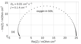
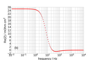
Figure 1: (a) Nyquist spectrum of the gas–diffusion layer impedance, Eq.(10). (b) Frequency dependence of the real part of impedance in (a). Parameters for calculations are listed in Table 1.

Impedance of oxygen transport in channel, Eq.(20), and in the cathode catalyst layer[2] also exhibit negative real part (Figure 2). Last but not least, in low–Pt cells, an important role plays oxygen transport through a thin Nafion film covering Pt/C agglomerates in the cathode catalyst layer[18, 19, 20]. The spectrum of this transport layer is quite similar in shape to the spectrum in Figure 1[14]. Thus, all the oxygen transport processes in a PEMFC cannot be described by the standard $RC$–kernel and another kernel suitable for description of impedance elements with the negative real part is needed.

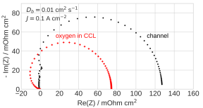
Figure 2: Nyquist spectra of the channel impedance, Eq.(20) and of impedance of oxygen transport in the CCL[2].

GDL thickness $l_{b}$, cm	0.023
Catalyst layer thickness $l_{t}$, cm	$10\cdot 10^{-4}$ (10 $\mu$m)
ORR Tafel slope $b$, mV	30
Double layer capacitance $C_{dl}$, F cm-3	20
GDL oxygen diffusivity $D_{b}$, cm2 s-1	0.01
Cell current density $J$, A cm-2	0.1
Pressure	Standard
Cell temperature $T$, K	273 + 80
Aur flow stoichiometry $\lambda$	2.0

Table 1: The base–case cell parameters used in calculations.

In a standard PEMFC, unless the cell current density is small, the DRT peaks of oxygen transport in the GDL, CCL and channel are expected to locate at frequencies below the frequency $f_{ct}$ of faradaic (charge transfer) processes. Thus, to capture the oxygen transport peaks, correction for negative real part of impedance is needed in the range of frequencies $f<f_{ct}$. The kernel $K_{2}$ suggested in his work consists, thus, of two parts:

$$K_{2}=\left\{\begin{split}&\dfrac{\tanh\sqrt{{\rm i}\omega\tau}}{\sqrt{{\rm i}\omega\tau}\left(1+{\rm i}\omega\tau\right)},\quad f\leq f_{*},\quad\text{TL kernel}\\ &\dfrac{1}{1+{\rm i}\omega\tau},\quad f>f_{*},\quad\text{$RC$ kernel}\end{split}\right.$$ (12)

where $f_{*}\simeq f_{ct}$ is the threshold frequency. Selection of optimal $f_{*}$ is discussed below. A function similar to impedance of a transport layer (TL) (10) forms the low–frequency part of $K_{2}$ ; the real part of this function is negative at $\omega\tau>1.81052$. The high–frequency ($RC$) part of $K_{2}$ is the standard $RC$–circuit kernel. Switching between TL and $RC$–kernels is necessary, as the TL–part itself does not describe well $RC$–circuit impedance (see below). The idea behind Eq.(12) is thus to expand the low–frequency components of cell impedance using the TL–kernel, and the high–frequency components using the standard $RC$–kernel.

It is convenient to combine Eq.(12) into one function

$$K_{2}=\dfrac{\tanh\left(\alpha\sqrt{{\rm i}\omega\tau}\right)}{\alpha\sqrt{{\rm i}\omega\tau}\left(1+{\rm i}\omega\tau\right)}$$ (13)

where $\alpha$ is a step function of the frequency $f$

$$\alpha=1-H(f-f_{*})+\epsilon,$$ (14)

$H(x)$ is the Heaviside step function and $\epsilon=10^{-10}$ is a small parameter to avoid zero division error. Parameter $\alpha$, therefore, changes from 1 to 0 at the threshold frequency $f=f_{*}$. With $\alpha\to 0$, the Warburg factor in Eq.(13) tends to unity:

$$\dfrac{\tanh\left(\alpha\sqrt{{\rm i}\omega\tau}\right)}{\alpha\sqrt{{\rm i}\omega\tau}}\to 1,\quad\text{as}\quad\alpha\to 0$$ (15)

and hence the $\alpha$–function serves as a switch between the two kernels in Eq.(12).

With Eq.(13), Eq.(5) takes the form

$$Z=R_{\infty}+R_{pol}\int_{-\infty}^{\infty}\dfrac{\tanh\left(\alpha\sqrt{{\rm i}\omega\tau}\right)G(\tau)\,d\ln(\tau)}{\alpha\sqrt{{\rm i}\omega\tau}\left(1+{\rm i}\omega\tau\right)}.$$ (16)

Setting in Eq.(16) $\omega\to 0$, it is easy to show that $G$ still obeys to normalization conditions Eq.(7).

III Numerical results and discussion

III.1 Synthetic impedance tests

Figure 3 shows imaginary part of $RC$–circuit impedance for $R=1$, $C=0.01$ and the DRT calculated using Eq.(16) and $\alpha=1$ for all frequencies (TL kernel). As can be seen, the main peak is positioned correctly at the frequency $1/(2\pi RC)$; however, the DRT spectrum exhibits three phantom peaks located to the right of the main peak. It is worth noting that quite similarly, the $RC$–kernel generates several phantom peaks in the DRT of Warburg finite–length impedance[13], i.e., no single kernel is able to represent correctly DRT of all impedance components.

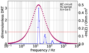
Figure 3: DRT (solid line, blue stars) and imaginary part of $RC$–circuit impedance $1/(1+10^{-2}{\rm i}\omega)$ (blue dots) calculated with Eq.(16) and $\alpha=1$ for all frequencies. Open red circles show imaginary part reconstructed from the calculated DRT using Eq.(16). Dashed red line – plot $\alpha=1$ for this calculation.

In a standard PEMFC, the characteristic frequencies of channel and GDL impedance are about 1 and 10 Hz, respectively[15]. Thus, the typical value of the threshold frequency $f_{*}$ in Eq.(14) should be about 10 Hz; however, the exact value can always be selected simply looking at the calculated DRT spectrum. In standard PEMFCs operated at oxygen stoichiometry of 2, the faradaic DRT peak is located to the right of the GDL transport peak on the log–frequency scale (see below).

Analytical impedance $\tilde{Z}_{tot}$ of the PEMFC cathode side has been obtained in[15] assuming fast proton and oxygen transport in the CCL. Equation for $\tilde{Z}_{tot}$ includes three components: impedance $\tilde{Z}_{chan}$ due to oxygen transport in channel, impedance $\tilde{Z}_{gdl}$ of oxygen transport in the GDL, and faradaic (charge–transfer) impedance $\tilde{Z}_{ct}$ The respective formulas are listed in Appendix; these solutions allow us to check how well DRT from Eq.(16) captures the channel, GDL and faradaic components in the total impedance $\tilde{Z}_{tot}$ spectrum (Figure 4).

The spectrum of $\tilde{Z}_{tot}$ has been calculated in the frequency range of $10^{-2}$ to $10^{4}$ Hz with 22 points per decade. Parameters for impedance calculation are listed in Table 1. Figure 4d depicts imaginary part of the impedance components calculated using equations in Appendix. Imaginary part of $\tilde{Z}_{tot}$ has then been used for calculation of DRT using our recent algorithm based on Tikhonov’s regularization and nonnegative least–squares (NNLS) solver[13, 14]. The NNLS method greatly outperforms projected gradient iterations suggested in[13]. In all the cases, the $L$–curve method gave the regularization parameter of $10^{-3}$.

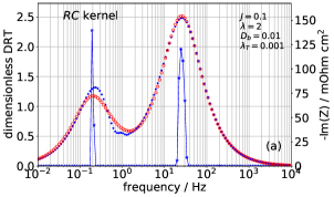
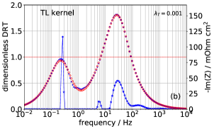
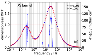
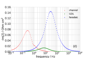
Figure 4: (a) DRT calculated using imaginary part of the total cathode side impedance, Eq.(25) (blue dots) with the $RC$–kernel (solid line). Red open circles – $\operatorname{Im}\left(Z_{tot}\right)$ reconstructed from the calculated DRT. (b) The same as in (a) curves obtained with the $TL$–kernel ($\alpha=1$) over the whole frequency range. Red dashed line indicates the plot of $\alpha$–function, Eq.(14). (c) The curves as in (a) obtained with the $K_{2}$–kernel and threshold frequency $f_{*}=10$ Hz. (d) Separate imaginary parts of the channel, GDL and faradaic impedance.

Figure 4a shows the DRT spectrum of $\tilde{Z}_{tot}$, Eq.(25), calculated using the $RC$–kernel. As can be seen, the standard kernel returns only two peaks corresponding to the channel (left peak) and faradaic (right peak) impedance. The GDL peak, which is clearly seen in Figure 4d is completely missing. Note poor quality of reconstructed imaginary part (red open circles) between 0.1 and 20 Hz. This is a result of poor description of the cell impedance by Eq.(5) in the frequency domain where the real part of GDL impedance is negative.

Figure 4b displays the DRT calculated with the ‘‘pure’’ TL–kernel, Eq.(12). The GDL peak is resolved and the quality of reconstructed imaginary part is much better; however, phantom high–frequency peaks to the right of the faradaic peak are clearly seen (cf. Figure 3). Figure 4c shows the DRT spectrum calculated using the $K_{2}$–kernel with the threshold frequency of 10 Hz; the GDL peak is well resolved and the phantom peaks vanish.

Table 2 shows the resistivities, Eq.(6), corresponding to individual peaks in Figure 4. As can be seen, $K_{2}$–kernel provides good estimate of the channel and faradaic resistivities; however, the GDL resistivity $R_{gdl}$ is underestimated by 30%. Nonetheless, as the contribution of $R_{gdl}$ is small, the 30%–accuracy could be tolerated.

	channel	GDL	faradaic
Exact	0.127	0.0250	0.300
RC–kernel	0.140	–	0.308
TL–kernel	0.125	0.0185	0.304∗
$K_{2}$–kernel	0.125	0.0171	0.305

Table 2: Channel, GDL and faradaic resistivities ($\Omega$ cm²) resulted from DRT, Eq.(6). Star ^∗ indicates the value calculated as a sum of faradaic and all high–frequency peaks in Figure 4b. The first row shows exact data calculated with Eqs.(32).

III.2 Real PEMFC spectra

A crucial check for the new kernel is calculation of DRT of a real PEM fuel cell. Impedance spectra of a standard Pt/C–based PEMFC have been measured in the frequency range of 0.1 to about $10^{3}$ Hz with 11 points per decade. The cell geometrical parameters and operating conditions are listed in Table 3; note that the air flow stoichiometry was 2 in this set of measurements. The impedance points in the frequency range above $\simeq 10^{3}$ Hz have been discarded due to effect of cable inductance. More details on experimental setup and measuring procedures can be found in[21].

GDL thickness $l_{b}$, cm	0.023
Catalyst layer thickness $l_{t}$, cm	$12\cdot 10^{-4}$ (12 $\mu$m)
Cell active area, cm2	76
Cathode pressure, kPa	150
Cathode flow RH	50%
Cell temperature $T$, K	273 + 80
H2/air flow stoichiometry $\lambda$	2 / 2

Table 3:

Figure 5 shows DRT spectra calculated with the real part of measured impedance using the $RC$–kernel. Figure 6 shows the respective peak frequencies and resistivities. The DRT spectra in Figures 5a–c exhibit four peaks, while in Figure 5d, the most high–frequency peak disappears. This peak represents proton transport in the CCL and at high cell currents it shifts to frequencies that have been discarded. The characteristic frequency $f_{4}$ of proton transport in the CCL is given by[22]

$$f_{4}\simeq\dfrac{2\sigma_{p}}{C_{dl}l_{t}^{2}}$$ (17)

With the typical values of $\sigma_{p}\simeq 0.01$ S cm^-1 and $C_{dl}\simeq 20$ F cm^-3 (Ref.[21]) we get $f_{p}\simeq 700$ Hz, which by the order of magnitude agrees with the proton peak position in Figures 5a–c. The growth of $f_{4}$ with the cell current and the respective decay of the peak resistivity $R_{4}$ (Figure 6c) is due to growing amount of liquid water improving the CCL proton conductivity.

The leftmost peak in Figures 5a–d represents impedance due to oxygen transport in the cathode channel. The characteristic frequency $f_{1}$ of this peak linearly increases with the cell current density (Figure 6a), which is a signature of channel impedance[15].

The highest, second peak in the DRT spectra (Figures 5a–d) represents the contributions of ORR and oxygen transport in the GDL (see below). In the absence of strong oxygen and proton transport limitations, the ORR resistivity is given by

$$R_{ORR}=\dfrac{b}{J}$$ (18)

which follows from the Tafel law. Qualitatively, the shape of second peak resistivity $R_{2}$ follows the trend of Eq.(18) due to dominating contribution of ORR resistivity to this peak (Figure 6b). Note that the separate GDL peak is not resolved by the $RC$–kernel.

The third, CCL–peak in Figures 5a–d is most probably due to oxygen transport in the CCL pores. For the estimate we take the Warburg finite–length formula for the transport layer frequency $f_{W}$

$$f_{W}=\dfrac{2.54D}{2\pi l^{2}}$$ (19)

where $D$ is the oxygen diffusivity in the transport layer of the thickness $l$. Setting $f_{W}=35$ Hz (Figure 5a) and $l=l_{t}$, for the oxygen diffusion coefficient in the CCL we get $D_{ox}\simeq 1.2\cdot 10^{-4}$ cm² s^-1, which agrees with measurements[21]. With the growth of cell current the peak frequency $f_{3}$ rapidly shifts to 200 Hz (Figure 6c), corresponding to $D_{ox}\simeq 7\cdot 10^{-4}$ cm² s^-1. The reason for this fast growth of $D_{ox}$ yet is unclear.

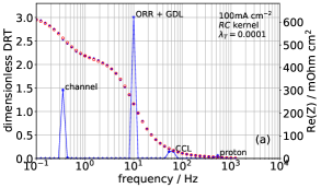
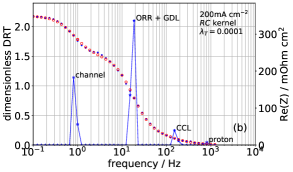
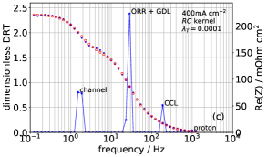
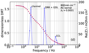
Figure 5: DRT (solid line) calculated using real part of the experimental PEMFC impedance (blue dots) with the $RC$–kernel for the current densities (a) 100, (b) 200, (c) 400, and (d) 800 mA cm^-2. Red open circles – $\operatorname{Re}\left(Z\right)$ reconstructed from the calculated DRT.

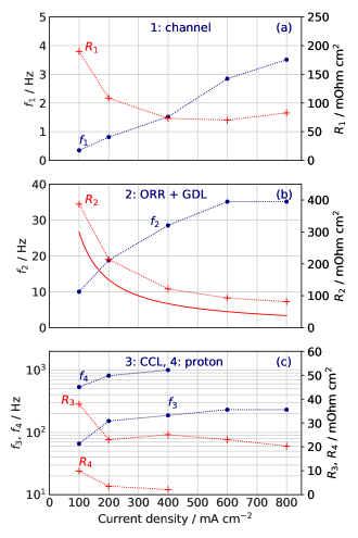
Figure 6: Frequency (blue curves, left axis) and resistivity (red curves, right axis) of the DRT peaks calculated using $RC$–kernel (Figure 5) vs mean cell current density $J$.

Figure 7 shows the DRT of the same impedance spectra calculated with the $K_{2}$ kernel. The properties of $K_{2}$ kernel are immediately seen: setting of the threshold frequency $f_{*}$ in Eq.(14) just to the left of the ‘‘ORR+GDL’’ peak in Figures 5a–d splits this peak into two well–resolved peaks (Figures 7a–d). The left peak of this doublet corresponds to the GDL impedance and the right peak to the ORR impedance. With the $K_{2}$–kernel, the proton transport peak is seen only at the smallest cell current density (Figure 7a), while at higher currents the peak vanishes indicating its shift to the frequencies above 1 kHz (Figures 7b–d).

The splitting the ‘‘CCL+GDL’’ peak into GDL and ORR peaks is confirmed by the behavior of peak resistivities in Figures 8b and c, respectively. The ORR peak resistivity $R_{3}$ follows the trend of Eq.(18) (solid line in Figure 8c) with the ORR Tafel slope $b=30$ mV, which is a typical value for Pt/C cells[23]. The GDL resistivity $R_{2}$ decreases in the range of cell currents 100 to 400 mA cm^-2 and remains nearly constant at higher currents (Figure 8b). Using again the Warburg formula Eq.(19), with $l=l_{b}=230\cdot 10^{-4}$ cm and the frequency between 10 to 30 Hz (Figure 8b), for the GDL oxygen diffusivity we get quite reasonable values of $D_{b}\simeq 0.013$–0.033 cm² s^-1. The increase of $D_{b}$ in the range of 100 to 400 mA cm^-2 is probably due to growing air flow velocity in the channel at the constant stoichiometry, which facilitates liquid droplets removal from the GDL.

$K_{2}$ kernel returns twice lower resustivity and about twice higher frequency of the CCL peak (cf. $f_{3}$, $R_{3}$ in Figure 6c and $f_{4}$, $R_{4}$ in Figure 8c). This shift leads to twice higher estimate of the CCL oxygen diffusivity, which is still acceptable (see above). Overall, confirmation of the CCL peak nature requires measurements at variable oxygen concentration and relative humidity.

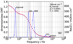
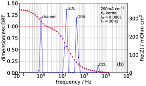
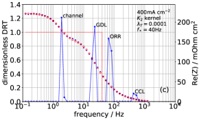
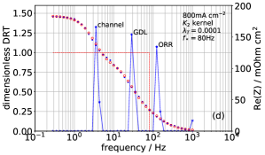
Figure 7: DRT (solid line) calculated using real part of the experimental PEMFC impedance (blue dots) with the $K_{2}$–kernel for the current densities (a) 100, (b) 200, (c) 400, and (d) 800 mA cm^-2. Red open circles – $\operatorname{Re}\left(Z\right)$ reconstructed from the calculated DRT. Dashed line shows the plot of $\alpha$, Eq.(14), switching the $K_{2}$–kernel from TL– to $RC$–one at the frequency marked by vertical line.

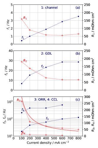
Figure 8: Frequency and resistivity of the DRT peaks calculated using $K_{2}$–kernel (Figure 7) vs mean cell current density $J$. Solid line in (c) is the Tafel ORR resistivity $R_{ORR}=b/J$ plotted with the Tafel slope $b=0.03$ V (69 mV/decade).

Over the past years, large efforts have been directed toward development of universal code capable to calculate DRT based on $RC$–kernel, not using any a priori information on the system (see a nice review of Effendy, Song and Bazant[24]). However, in PEMFC studies it would be wasteful to ignore analytical results showing that the $RC$–kernel alone is not well suited for DRT description of the spectra.

IV Conclusions

Impedance of all oxygen transport processes in a PEM fuel cell exhibits negative real part in some frequency range. This makes it difficult accurate calculation of the respective DRT peaks using the standard $RC$–kernel $1/(1+{\rm i}\omega\tau)$. A novel kernel $K_{2}$, Eq.(13), is suggested. $K_{2}$ combines the low–frequency transport layer kernel having a domain with negative real part, and the standard $RC$–kernel for description of faradaic and high–frequency processes in the cell. Calculation of DRT for analytical PEMFC impedance shows that $K_{2}$ kernel captures the peak due to oxygen transport in the gas–diffusion layer, while the $RC$–kernel can miss this peak. Comparison of Pt/C PEMFC DRT calculated using $RC$– and $K_{2}$–kernel shows that the $K_{2}$–kernel resolves the GDL oxygen transport peak, which otherwise is merged to the ORR peak when using the standard $RC$–kernel. Overall, the $K_{2}$–spectra of a standard Pt/C PEMFC operating at the air flow stoichiometry $\lambda=2$ consist of five peaks. In the frequency ascending order, these peaks are due to (1) oxygen transport in channel, (2) oxygen transport in the GDL, (3) faradaic reactions, (4) oxygen transport in the CCL, and (5) proton transport in the CCL. If the CCL proton conductivity is high, the peak (5) shifts to the frequencies well above 1 kHz, and it may not be resolved due to inductance of measuring system.

Appendix A Model equations for GDL, channel and faradaic impedance

Equations of this Section have been derived in[15].

• Channel impedance is

  $$\tilde{Z}_{chan}=-\dfrac{4\lambda{{\rm e}^{\tilde{\eta}_{0}}}N_{c}}{\bigl{(}2\lambda{\rm i}\tilde{\omega}+(2\lambda-1){{\rm e}^{\tilde{\eta}_{0}}}\bigr{)}D_{c}}$$ (20)

  where

  $$N_{c}=\lambda^{2}\tilde{J}\left({{\rm e}^{2\tilde{\eta}_{0}}}+\left(\tilde{J}+{\rm i}\tilde{\omega}(1+\xi^{2})\right)\times{{\rm e}^{\tilde{\eta}_{0}}}-\xi^{2}\tilde{\omega}^{2}\right)\\ \times\exp\left(\dfrac{-{{\rm e}^{\tilde{\eta}_{0}}}-{\rm i}\tilde{\omega}\xi^{2}}{\lambda\tilde{J}}\right)+\lambda\left({{\rm e}^{\tilde{\eta}_{0}}}-\lambda\tilde{J}+{\rm i}\tilde{\omega}\xi^{2}\right)\\ \times\left({{\rm e}^{2\tilde{\eta}_{0}}}+\left(\tilde{J}+{\rm i}\tilde{\omega}(\xi^{2}+1)\right){{\rm e}^{\tilde{\eta}_{0}}}-\xi^{2}\tilde{\omega}^{2}\right)\\ -\left({{\rm e}^{\tilde{\eta}_{0}}}+{\rm i}\tilde{\omega}\xi^{2}\right)^{2}{{\rm e}^{\tilde{\eta}_{0}}}/2$$ (21)

  $$D_{c}=2\lambda^{2}\tilde{J}\left({{\rm e}^{2\tilde{\eta}_{0}}}+\left(\tilde{J}+{\rm i}\tilde{\omega}(1+\xi^{2})\right){{\rm e}^{\tilde{\eta}_{0}}}-\xi^{2}\tilde{\omega}^{2}\right)\\ \times\exp\left(\dfrac{-{{\rm e}^{\tilde{\eta}_{0}}}-{\rm i}\tilde{\omega}\xi^{2}}{\lambda\tilde{J}}\right){{\rm e}^{\tilde{\eta}_{0}}}-2\lambda\xi^{6}\tilde{\omega}^{4}\\ +{\rm i}\left(2\lambda\xi^{2}-\xi^{2}+4\lambda\right)\xi^{4}{{\rm e}^{\tilde{\eta}_{0}}}\,\tilde{\omega}^{3}\\ +2\xi^{2}\left(\left(2\lambda\xi^{2}-\xi^{2}+\lambda\right){{\rm e}^{\tilde{\eta}_{0}}}+\lambda^{2}\tilde{J}\right){{\rm e}^{\tilde{\eta}_{0}}}\tilde{\omega}^{2}\\ -{\rm i}\left(\left(2\lambda-1\right)\xi^{2}{{\rm e}^{\tilde{\eta}_{0}}}+2\lambda\tilde{J}\left(\lambda\xi^{2}-\xi^{2}+\lambda\right)\right){{\rm e}^{2\tilde{\eta}_{0}}}\tilde{\omega}\\ -2\lambda\tilde{J}\left(\left(\lambda-1\right){{\rm e}^{\tilde{\eta}_{0}}}+\lambda\tilde{J}\right){{\rm e}^{2\tilde{\eta}_{0}}}.$$ (22)

  and parameters $\xi$ and $\lambda$ are given by

  $$\xi=\sqrt{\dfrac{4Fhc_{h}^{in}}{C_{dl}l_{t}b}},\quad\lambda=\dfrac{4Fhvc_{h}^{in}}{LJ}.$$ (23)

• GDL impedance is given by Eq.(10).

• Faradaic impedance is

  $$\tilde{Z}_{ct}=\dfrac{1}{{\rm i}\tilde{\omega}+\left(1-\dfrac{1}{2\lambda}\right){{\rm e}^{\tilde{\eta}_{0}}}}$$ (24)

• Total impedance of the cathode side, including channel, GDL and faradaic components

  $$\tilde{Z}_{tot}=\dfrac{\lambda B^{3}}{D_{tot}}\left(\cosh(\phi)+\dfrac{{{\rm e}^{\tilde{\eta}_{0}}}\sinh(\phi)}{\psi}\right)$$ (25)

  where

  $$D_{tot}=\lambda^{2}\tilde{J}{{\rm e}^{\tilde{\eta}_{0}}}\left(\lambda\tilde{J}A+BC\right)\left(\exp\left(\dfrac{B}{\lambda\tilde{J}}\right)-1\right)\\ +\left(({\rm i}\tilde{\omega}+{{\rm e}^{\tilde{\eta}_{0}}})\lambda-{{\rm e}^{\tilde{\eta}_{0}}}/2\right)B^{3}\cosh(\phi)\\ -\lambda{{\rm e}^{\tilde{\eta}_{0}}}B\left(\lambda\tilde{J}A+B(A/2+C)\right)$$ (26)

  and the coefficients $A$, $B$ and $C$ are given by

  $$A=\dfrac{\psi{{\rm e}^{\tilde{\eta}_{0}}}}{\lambda\cosh(\phi)\left(\psi+{{\rm e}^{\tilde{\eta}_{0}}}\tanh(\phi)\right)}$$ (27)

  $$B=-{\rm i}\tilde{\omega}\xi^{2}-\psi\tanh(\phi)-\dfrac{\lambda A}{\cosh(\phi)}$$ (28)

  $$C=-\dfrac{\psi\left({\rm i}\tilde{\omega}+{{\rm e}^{\tilde{\eta}_{0}}}\right)}{\cosh(\phi)\left(\psi+{{\rm e}^{\tilde{\eta}_{0}}}\tanh(\phi)\right)}$$ (29)

  Auxiliary parameters $\phi$ and $\xi$ are given by

  $$\begin{split}&\phi=\mu\tilde{l}_{b}\sqrt{{\rm i}\tilde{\omega}/\tilde{D}_{b}}\\ &\psi=\mu\sqrt{{\rm i}\tilde{\omega}\tilde{D}_{b}}\end{split}$$ (30)

• The cell polarization curve is

  $${{\rm e}^{\tilde{\eta}_{0}}}=-\lambda\ln\left(1-\dfrac{1}{\lambda}\right)\tilde{J}$$ (31)

• GDL $R_{gdl}$, faradaic $R_{f}$ and channel $R_{chan}$ resistivities in the dimension form ($\Omega$ cm²):

  $$\begin{split}&R_{gdl}=\dfrac{bl_{b}}{4FD_{b}c_{h}^{in}},\\ &R_{f}=\dfrac{b}{J}\\ &R_{chan}=-\dfrac{b}{J\,(2\lambda-1)}\biggl{(}2\lambda^{2}\ln\left(1-\dfrac{1}{\lambda}\right)^{2}\\ &\qquad-\lambda\ln\left(1-\dfrac{1}{\lambda}\right)-\dfrac{2}{\ln(1-1/\lambda)}\biggr{)}.\end{split}$$ (32)

Nomenclature

$\tilde{}$	Marks dimensionless variables
$b$	ORR Tafel slope, V
$C_{dl}$	Double layer volumetric capacitance, F cm-3
$c_{1}$	Oxygen molar concentration
	at the CCL/GDL interface, mol cm-3
$c_{b}$	Oxygen molar concentration in the GDL, mol cm-3
$c_{h}$	Oxygen molar concentration in the channel, mol cm-3
$c_{h}^{in}$	Reference (inlet) oxygen concentration, mol cm-3
$D_{b}$	Oxygen diffusion coefficient in the GDL, cm2 s-1
$F$	Faraday constant, C mol-1
$f$	Characteristic frequency, Hz
$i_{*}$	ORR volumetric exchange current density, A cm-3
${\rm i}$	Imaginary unit
$j$	Local proton current density along the CCL, A cm-2
$j_{\lim}$	Limiting current density
	due to oxygen transport in the GDL, Eq.(LABEL:eq:jlim) A cm-2
$j_{0}$	Local cell current density, A cm-2
$l_{b}$	GDL thickness, cm
$l_{t}$	CCL thickness, cm
$t$	Time, s
$t_{*}$	Characteristic time, s, Eq.(9)
$x$	Coordinate through the cell, cm
$Z$	Local impedance, Ohm cm2
$Z_{gdlc}$	GDL+channel impedance, Ohm cm2
$Z_{tot}$	Total cathode side impedance, including
	faradaic one, Ohm cm2
$z$	Coordinate along the cathode channel, cm

Subscripts:

$0$	Membrane/CCL interface
$1$	CCL/GDL interface
$b$	In the GDL
$gdl$	GDL
$gdlc$	GDL+channel
$f$	faradaic
$h$	Air channel
$W$	Warburg

Superscripts:

$0$	Steady–state value
$1$	Small–amplitude perturbation

Greek:

$\eta$	ORR overpotential, positive by convention, V
$\lambda$	Air flow stoichiometry, Eq.(23)
$\lambda_{T}$	Tikhonov regularization parameter
$\mu$	Dimensionless parameter, Eq.(11)
$\xi$	Dimensionless parameter, Eq.(23)
$\phi$	Dimensionless parameter. Eq.(30)
$\psi$	Dimensionless parameter. Eq.(30)
$\omega$	Angular frequency of the AC signal, s-1

References

- Lasia [2014] A. Lasia. Electrochemical Impedance Spectroscopy and its Applications. Springer, New York, 2014.
- Kulikovsky [2016] A. A. Kulikovsky. Analytical physics–based impedance of the cathode catalyst layer in a PEM fuel cell at typical working currents. Electrochim. Acta, 225:559–565, 2016. doi: 10.1016/j.electacta.2016.11.129.
- Barsoukov and Macdonald [2018] E. Barsoukov and J. R. Macdonald. Impedance Spectroscopy: Theory, Experiment, and Applications. John Wiley & Sons, New Jersey, 3 edition, 2018.
- Fuoss and Kirkwood [1941] R.M. Fuoss and J.G. Kirkwood. Electrical properties of solids. viii. Dipole moments in polyvinyl chloride-diphenyl systems. J. Am. Chem. Soc., 63:385–394, 1941. doi: 10.1021/ja01847a013.
- Schichlein et al. [2002] H. Schichlein, A. C. Müller, M. Voigts, A. Krügel, and E. Ivers-Tiffée. Deconvolution of electrochemical impedance spectra for the identification of electrode reaction mechanisms in solid oxide fuel cells. J. Appl. Electrochem., 32:875–882, 2002. doi: 10.1023/A:1020599525160.
- Ivers-Tiffée and Weber [2017] E. Ivers-Tiffée and A. Weber. Evaluation of electrochemical impedance spectra by the distribution of relaxation times. J. Ceramic Soc. Japan, 125:193–201, 2017. doi: 10.2109/jcersj2.16267.
- Heinzmann et al. [2018] M. Heinzmann, A. Weber, and E. Ivers-Tiffée. Advanced impedance study of polymer electrolyte membrane single cells by means of distribution of relaxation times. J. Power Sources, 402:24 – 33, 2018. doi: 10.1016/j.jpowsour.2018.09.004.
- Cohen et al. [2021] G. A. Cohen, D. Gelman, and Y. Tsur. Development of a typical distribution function of relaxation times model for polymer electrolyte membrane fuel cells and quantifying the resistance to proton conduction within the catalyst layer. J./ Phys./Chem./ C, 125:11867–11874, 2021. doi: 10.1021/acs.jpcc.1c03667.
- Reshetenko and Kulikovsky [2021] T. Reshetenko and A. Kulikovsky. Understanding the distribution of relaxation times of a low–Pt PEM fuel cell. Electrochim. Acta, 391:138954, 2021. doi: 10.1016/j.electacta.2021.138954.
- Wang et al. [2021] Q. Wang, Z. Hu, L. Xu, Q. Gan, J. Li 1, X. Du, and M. Ouyang. A comparative study of equivalent circuit model and distribution of relaxation times for fuel cell impedance diagnosis. Int. J. Energy Res., 45:15948–15961, 2021. doi: 10.1002/er.6825.
- Wan et al. [2015] T. H. Wan, M. Saccoccio, C. Chen, and F. Ciucci. Influence of the discretization methods on the distribution of relaxation times deconvolution: Implementing radial basis functions with DRTtools. Electrochim. Acta, 184:483–499, 2015. doi: 10.1016/j.electacta.2015.09.097.
- Hershkovitz et al. [2011] S. Hershkovitz, S. Tomer, S. Baltianski, and Y. Tsur. Isgp: Impedance spectroscopy analysis using evolutionary programming procedure. ECS Trans., 33:67–73, 2011. doi: 10.1149/1.3589186.
- Kulikovsky [2020a] Andrei Kulikovsky. PEM fuel cell distribution of relaxation times: A method for calculation and behavior of oxygen transport peak. Phys. Chem. Chem. Phys., 22:19131–19138, 2020a. doi: 10.1039/D0CP02094J.
- Kulikovsky [2021a] Andrei Kulikovsky. Impedance and resistivity of low–Pt cathode in a PEM fuel cell. J. Electrochem. Soc., 168:044512, 2021a. doi: 10.1149/1945-7111/abf508.
- Kulikovsky [2021b] A. Kulikovsky. Analytical impedance of oxygen transport in the channel and gas diffusion layer of a PEM fuel cell. J. Electrochem. Soc., (submitted), 2021b.
- Kulikovsky and Shamardina [2015] A. Kulikovsky and O. Shamardina. A model for PEM fuel cell impedance: Oxygen flow in the channel triggers spatial and frequency oscillations of the local impedance. J. Electrochem. Soc., 162:F1068–F1077, 2015. doi: 10.1149/2.0911509jes.
- Warburg [1899] E. Warburg. Über das Verhalten sogenannter unpolarisirbarer Electroden gegen Wechselstrom. Ann. Physik und Chemie, 67:493–499, 1899. doi: 10.1002/andp.18993030302.
- Greszler et al. [2012] T. A. Greszler, D. Caulk, and P. Sinha. The impact of platinum loading on oxygen transport resistance. J. Electrochem. Soc., 159:F831–F840, 2012. doi: 10.1149/2.061212jes.
- Weber and Kusoglu [2014] A. Z. Weber, the CCL transport peak shifts to higher frequencies, while and A. Kusoglu. Unexplained transport resistances for low–loaded fuel–cell catalyst layers. J. Mater. Chem. A, 2:17207–17211, 2014. doi: 10.1039/c4ta02952f.
- Kongkanand and Mathias [2016] A. Kongkanand and M. F. Mathias. The priority and challenge of high-power performance of lowplatinum proton-exchange membrane fuel cells. Phys. Chem. Lett., 7:1127–1137, 2016. doi: 10.1021/acs.jpclett.6b00216.
- Reshetenko and Kulikovsky [2019] T. Reshetenko and A. Kulikovsky. A model for local impedance: Validation of the model for local parameters recovery from a single spectrum of PEM fuel cell. J. Electrochem. Soc., 166:F431–F439, 2019. doi: 10.1149/2.1241906jes.
- Kulikovsky [2020b] Andrei Kulikovsky. Analysis of proton and electron transport impedance of a PEM fuel cell in H2/N2 regime. Electrochem. Sci. Adv., e202000023, 2020b. doi: 10.1002/elsa.202000023.
- Neyerlin et al. [2006] K. C. Neyerlin, W. Gu, J. Jorne, and H. Gasteiger. Determination of catalyst unique parameters for the oxygen reduction reaction in a PEMFC. J. Electrochem. Soc., 153:A1955–A1963, 2006. doi: 10.1149/2.0471803jes.
- Effendy et al. [2020] S. Effendy, J. Song, and M. Z. Bazant. Analysis, design, and generalization of electrochemical impedance spectroscopy (EIS) inversion algorithms. J. Electrochem. Soc., 167:106508, 2020. doi: 10.1149/1945-7111/ab9c82.