Polarised W+j production at the LHC:
a study at NNLO QCD accuracy

Abstract

We study polarisation of W-bosons produced in association with one jet at the LHC. In particular, we provide all necessary theoretical ingredients for the precise extraction of polarisation fractions. To that end, we present new polarised predictions up to NNLO QCD accuracy employing the narrow-width approximation, in two phase spaces: inclusive and fiducial. We compare results in the fiducial phase space to a full off-shell computation as well as experimental data. Finally, we fit the polarisation fractions using shape templates and show that NNLO corrections significantly improve their determination.

1 Introduction

High-energy collisions of protons at the Large Hadron Collider (LHC) allow for a copious production of W-bosons in association with one or more high-$p_{\rm T}$ jets. In fact, this class of processes has one of the highest cross sections for electroweak (EW) boson production and therefore constitutes an important background to many other Standard Model processes. This motivated numerous theoretical and experimental works Azzurri:2020lbf .

By scrutinising the longitudinal mode, which originates from the electroweak symmetry breaking (EWSB) mechanism, one gets an insight into the EW sector with possible footprints of new-physics effects. This idea has lead to numerous massive vector boson polarisation studies for different LHC processes, including Drell-Yan Manca:2017xym , diboson production Baglio:2018rcu ; Baglio:2019nmc ; Denner:2020bcz ; Denner:2020eck ; Denner:2021csi , and vector-boson scattering Ballestrero:2017bxn ; Ballestrero:2019qoy ; Ballestrero:2020qgv . The production of a polarised W-boson in association with one jet represents another important handle to pinpoint the SM, and it has therefore received its due attention in the scientific community Bern:2011ie ; Stirling:2012zt ; Belyaev:2013nla , and several dedicated experimental measurements ATLAS:2012au ; CMS:2011kaj were carried out.

From a theoretical point of view, $\text{W}\!+\text{j}$ production is a rather well understood process, with NNLO QCD predictions Boughezal:2015dva ; Boughezal:2016dtm ; Gehrmann-DeRidder:2019avi , EW corrections Kuhn:2007qc ; Kuhn:2007cv ; Hollik:2007sq ; Denner:2009gj , and combinations thereof Kallweit:2014xda ; Kallweit:2015dum ; Biedermann:2017yoi ; Lindert:2017olm being already available. Nonetheless, predictions for the polarised W-bosons have so far been limited to NLO QCD accuracy Bern:2011ie ; Stirling:2012zt .

In this work, we are filling this gap by providing, for the first time, the NNLO QCD predictions for the polarised W-bosons in the narrow-width approximation (NWA) at the LHC running at 13  TeV. We perform this computation in two different phase spaces: inclusive and fiducial. The inclusive phase space gives a clean and a more holistic picture of polarisation features, whereas the fiducial phase space mimics a realistic measurement and helps understand the limitations of the NWA and boson-polarisation definition. Thus, in the fiducial phase space, we also compare the obtained NWA predictions with the full off-shell computation as well as with experimental data provided by the CMS collaboration CMS:2017gbl . The first comparison provides a realistic quality check of the NWA, which plays a crucial role in the definition of the polarised states. Finally, we use polarised distributions, obtained at amplitude level, as templates to fit the polarisation fractions to the data, and show that NNLO corrections significantly improve their precise determination.

The article is organised as follows: in section 2 we introduce the process under consideration and goes over details of our computation. We list numerical inputs used as well as technical details for both phase spaces. We provide information on the implementation and list validations that we have carried out. Section 3 presents results of the computation. This includes: theoretical predictions for the polarised W-boson in the form of cross sections and differential distributions, polarisation fractions, comparison to off-shell simulations and data, and finally, fits that can be used to extract polarisation fractions. We summarise our findings and make concluding remarks in section 4.

2 Setup

2.1 Definition of the process

In this work, the hadronic processes under investigation are

$$\text{p}\text{p}\rightarrow\ell^{\pm}\,\overset{\scriptscriptstyle(-)}{\nu}_{\!\!\!\ell}\,\text{j}\;,$$ (1)

and are usually referred to as $\text{W}\!+\text{j}$ production. In this study, given that we consider massless leptons, both cases $\ell=\text{e},\mu$ are equivalent. In figure 1, two LO diagrams for the “plus” signature are represented. The LO is defined at order $\mathcal{O}{\left(\alpha^{2}\alpha_{\text{s}}\right)}$, while the NLO and NNLO QCD corrections are defined at orders $\mathcal{O}{\left(\alpha^{2}\alpha_{\text{s}}^{2}\right)}$ and $\mathcal{O}{\left(\alpha^{2}\alpha_{\text{s}}^{3}\right)}$, respectively. Further on, we will use the following notation for the cross sections and their perturbative expansions:

$$\sigma(\text{p}\text{p}\rightarrow\ell^{\pm}\,\overset{\scriptscriptstyle(-)}{\nu}_{\!\!\!\ell}\,\text{j}) \equiv\sigma^{\pm}=\sigma^{\pm(0)}+\sigma^{\pm(1)}+\sigma^{\pm(2)}+\order{\alpha_{\text{s}}^{4}}\,.$$ (2)

Also, we consider both the “plus” and “minus” signatures separately unless explicitly stated otherwise, so we will omit the $\pm$ superscript for brevity. Finally, we define

$$\sigma^{\pm}_{\rm LO} =\sigma^{\pm(0)}\,,$$

$$\sigma^{\pm}_{\rm NLO} =\sigma^{\pm(0)}+\sigma^{\pm(1)}\,,$$

$$\sigma^{\pm}_{\rm NNLO} =\sigma^{\pm(0)}+\sigma^{\pm(1)}+\sigma^{\pm(2)}\,,$$ (3)

and the corresponding $K$-factors to express perturbative corrections as

$$K^{\pm}_{\rm NLO}=\frac{\sigma^{\pm}_{\rm NLO}}{\sigma^{\pm}_{\rm LO}}\,,\quad K^{\pm}_{\rm NNLO}=\frac{\sigma^{\pm}_{\rm NNLO}}{\sigma^{\pm}_{\rm NLO}}\,.$$ (4)

The same notation will be used analogously in differential cross sections. $K$-factors are generally given with respect to the central scale choice, and scale variations are given by variations in the numerator only.

Figure 1: Leading-order Feynman diagrams of the hadronic process $\text{p}\text{p}\rightarrow\ell^{+}\,\nu_{\ell}\text{j}$.

In addition, to QCD corrections, the EW ones are also phenomenologically relevant. For $\text{W}\!+\text{j}$ production at the LHC, they are typically at the level of a few per cent for total cross sections but can reach several dozen per cent in the high energy limits Denner:2009gj . For $\text{W}\!+\text{j}$ polarised predictions, EW corrections are unknown. The study of the impact of EW corrections for $\text{W}\!+\text{j}$ polarised predictions is thus left for future work. In this work, we focus exclusively on the effect of QCD corrections.

In order to define the cross sections for polarised W-bosons, we need to define polarisation states of the propagating bosons. This requires the bosons to be on their mass shell. To this end, we employ the NWA which allows to factorise the production and decay of on-shell bosons, while keeping all spin information. For the process at hand, this approximation does not lead to a reduction of the number of Feynman diagrams to be considered. Indeed, in the present case, the leptonic pair consisting of a neutrino and a charged lepton can only be obtained through decay of the W-boson, in contrast to processes involving neutral currents. Considering the NWA, we write tree-level amplitudes, as well as virtual and higher-multiplicities amplitudes, in the following way:

$$\mathcal{M}^{\rm NWA}(\text{p}\text{p}\rightarrow\ell^{\pm}\,\overset{\scriptscriptstyle(-)}{\nu}_{\!\!\!\ell}\,\text{j})=\frac{1}{M_{W}\Gamma_{W}}\sum_{h\in\Lambda}\mathcal{M}_{h}(\text{p}\text{p}\to\text{W}\text{j})\cdot\Gamma_{h}\left(\text{W}\to\ell^{\pm}\,\overset{\scriptscriptstyle(-)}{\nu}_{\!\!\!\ell}\right),$$ (5)

where $h$ represents polarisations from the set $\Lambda=\{+1,-1,0\}$. The ‘transversely polarised’ amplitudes is represented by $\Lambda={\mathrm{T}}=\{+1,-1\}$ and the ‘longitudinally polarised’ by $\Lambda={\mathrm{L}}=\{0\}$. By squaring this amplitude, one obtains unpolarised cross sections. In turn, polarised cross sections are retrieved by squaring only one polarised amplitude. It implies that the sum of the polarised cross sections and the unpolarised ones differ by the interference contributions between the different polarised amplitudes. Such effects are analysed in details in section 3.3.

The definition of boson polarisation is not unique. To be exact, with W-boson momentum in the laboratory frame $p=(E,\vec{p})=(E,|\vec{p}|\sin\theta\cos\phi,|\vec{p}|\sin\theta\sin\phi,|\vec{p}|\cos\theta)$, we define the polarisation vector using the helicity frame Bern:2011ie ; Poncelet:2021jmj as follows:

$$\varepsilon^{\mu}_{-} =\frac{1}{\sqrt{2}}\left(0,\cos\theta\cos\phi+\mathrm{i}\sin\phi,\cos\theta\sin\phi-\mathrm{i}\cos\phi,-\sin\theta\right),$$

$$\varepsilon^{\mu}_{+} =\frac{1}{\sqrt{2}}\left(0,-\cos\theta\cos\phi+\mathrm{i}\sin\phi,-\cos\theta\sin\phi-\mathrm{i}\cos\phi,\sin\theta\right),$$

$$\varepsilon^{\mu}_{0} =\frac{1}{m_{W}}\left(|\vec{p}|,E\sin\theta\cos\phi,E\sin\theta\sin\phi,E\cos\theta\right).$$ (6)

To quantify the contribution of a particular polarisation to the (differential) cross section we use polarisation fractions

$$f_{p}=\frac{\sigma_{p}}{\sum_{p}\sigma_{p}}\quad\text{for}\quad p\in\{\rm L,T\}\,,$$ (7)

where $\sigma_{p}$ is the cross section with polarisation $p$. For estimating the scale uncertainty in the ratio, we use an uncorrelated estimation, that is we perform the squared error propagation of independent scale variations in both the numerator and denominator.

2.2 Numerical inputs and event selections

Numerical inputs

Our computation simulates $\text{p}\text{p}\rightarrow\ell^{\pm}\,\overset{\scriptscriptstyle(-)}{\nu}_{\!\!\!\ell}\,\text{j}$ processes at the LHC running with the centre-of-mass energy of $\sqrt{s}=13\,\text{TeV}$. The parton distribution functions (PDF) used are the NNPDF31_as_0118 set NNPDF:2017mvq with corresponding orders. Throughout the computation we use the $n_{f}=5$ scheme. The input masses and widths are

$$M_{\text{W}}^{\text{OS}} =80.3790\,\text{GeV},\qquad \Gamma_{\text{W}}^{\text{OS}} =2.0850\,\text{GeV},$$ (8)

$$M_{\text{Z}}^{\text{OS}} =91.1876\,\text{GeV},\qquad \Gamma_{\text{Z}}^{\text{OS}} =2.4952\,\text{GeV}.$$ (9)

They determine the pole boson parameters actually used in the numerical evaluation of the matrix elements Bardin:1988xt :

$$M_{\mathrm{V}}=\frac{M_{V}^{\text{OS}}}{\sqrt{1+(\Gamma_{V}^{\text{OS}}/M_{V}^{\text{OS}})^{2}}},\qquad\Gamma_{\mathrm{V}}=\frac{\Gamma_{V}^{\text{OS}}}{\sqrt{1+(\Gamma_{V}^{\text{OS}}/M_{V}^{\text{OS}})^{2}}},$$ (10)

for ${\mathrm{V}}=\text{W},\text{Z}$. The electromagnetic coupling is fixed following the $G_{\mu}$ scheme Denner:2000bj with

$$G_{\mathrm{F}}=1.16638\times 10^{-5}\,\text{GeV}^{-2}.$$ (11)

All leptons are considered massless and we assume the diagonal CKM matrix.

The central choice used for both factorisation and renormalisation scale reads

$$\mu=\frac{1}{2}H_{\mathrm{T}}^{\prime}=\frac{1}{2}\left(\sqrt{M_{\text{W}}^{2}+p^{2}_{{\mathrm{T}},\text{W}}}+\sum_{i=\textrm{jets}}p_{{\mathrm{T}},i}\right),$$ (12)

where the sum goes over all jets obtained after applying the jet algorithm. For the estimate of the missing higher orders, we adopt the standard 7-point scale variation prescription.

Phase-space definitions

In the present work, we consider two phase spaces that we refer to as inclusive and fiducial setup, respectively.

In both cases, we use the anti-$k_{\text{T}}$ algorithm Cacciari:2008gp with $R=0.4$ to identify QCD jets. We require at least one jet fulfilling

$$\absolutevalue{y_{\text{j}}}<2.4\quad\textrm{and}\quad p_{{\mathrm{T}},\text{j}}>30\,\text{GeV}.$$ (13)

• Inclusive setup:
  The inclusive setup does not have any cuts apart from the jet acceptance criteria in eq. (13).

• Fiducial setup:
  To emulate a realistic experimental setup, we follow the selection procedure used in the recent CMS study CMS:2017gbl . In addition to eq. (13), jets are required to have

  $$\Delta R(\ell,j)>0.4,$$ (14)

  where $\ell$ is the charged lepton originating from the boson decay. Furthermore, the following requirements are applied to the leptonic products:

  $$p_{{{\mathrm{T}}},\ell}>25\,\text{GeV},\qquad|\eta_{\ell}|<2.5,\qquad M_{{\mathrm{T}}}(\text{W})>50\,\text{GeV},$$ (15)

  where the W-boson transverse mass is defined as

  $$m_{{\mathrm{T}}}^{\text{W}}=\sqrt{M_{\text{W}}^{2}+p_{{\mathrm{T}},\text{W}}^{2}}=\sqrt{2p_{{{\mathrm{T}}},\ell}\cdot p_{{\mathrm{T}},\text{miss}}\left(1-\cos\Delta\phi\right)},$$ (16)

  with $\Delta\phi=\min\left(|\phi_{\ell}-\phi_{\nu}|,2\pi-|\phi_{\ell}-\phi_{\nu}|\right)$ being the azimuthal separation of the lepton and neutrino momenta. We define $p_{{\mathrm{T}},\text{miss}}$ using the neutrino momentum.

2.3 Implementation and validation procedures

The computation has been carried out using the Stripper framework which is a C++ implementation of the four-dimensional formulation of the sector-improved residue subtraction scheme Czakon:2010td ; Czakon:2014oma ; Czakon:2019tmo . The Stripper library consists in a Monte-Carlo generator which automates the subtraction procedure. For the computation of matrix elements, it relies on external programs. Tree-level amplitudes, are calculated using AvH library Bury:2015dla . The one-loop amplitudes are calculated using our privately extended version of O PEN L OOPS 2 Cascioli:2011va ; Buccioni:2017yxi ; Buccioni:2019sur , which is capable of calculations with defined polarisations. The two-loop helicity amplitudes for the off-shell calculation and the necessary components for the polarised studies were extracted from ref. Gehrmann:2011ab . The adaptation of these amplitudes to on-shell polarised bosons can be found in the appendix A.

The validity of this calculation is supported by the following considerations and cross checks. The calculation exploits the same framework that was used for the NNLO QCD study of $\text{W}\!+\!\text{c}$ Czakon:2020coa and the polarised $\text{W}^{+}\text{W}^{-}$ production Poncelet:2021jmj . The latter study also explored the effectiveness of the NWA approach in the polarisation setting. Details about the implementation of the NWA can be found in ref. Czakon:2020qbd . All 0-, 1-, and 2-loop on-shell amplitudes were checked against full off-shell amplitudes at on-shell phase space points. The 0- and 1- loop polarised amplitudes were also cross-checked between AvH, O PEN L OOPS 2, Recola Actis:2012qn ; Actis:2016mpe , and ref. Gehrmann:2011ab . Finally, we produced polarised predictions at NLO following the setup of ref. Bern:2011ie and found perfect agreement with their results.

3 Results

In this section we present and analyse results of our numerical simulations. At first, we discuss polarisation setups in section 3.1. Then we explore the differences between the “plus” and “minus” signature in section 3.2. Further on, we discuss off-shell and interference effects and compare our predictions against experimental data of the CMS collaboration CMS:2017gbl . Finally, we perform a fit of these experimental data using the polarised shape distributions we have computed in the previous parts.

3.1 Polarised predictions

As explained in section 2, once a W-boson is on its mass shell, it is possible to define its longitudinal (L) and transverse (T) polarisations. The total cross sections of such polarised predictions for both the inclusive and fiducial setups are presented in tables 1 and 2, respectively.

Inc.	LO [fb]	NLO [fb]	$K_{\text{NLO}}$	NNLO [fb]	$K_{\text{NNLO}}$	$f_{\text{NNLO}}$
$\text{W}^{+}_{\rm L}$	$162.964(8)^{+11.5\%}_{-9.4\%}$	$268.4(2)^{+9.4\%}_{-8.0\%}$	1.65	$287.8(10)^{+1.3\%}_{-2.8\%}$	1.07	$0.186(2)^{+3.2\%}_{-3.1\%}$
$\text{W}^{+}_{\rm T}$	$827.00(7)^{+11.4\%}_{-9.3\%}$	$1214.5(5)^{+7.6\%}_{-6.8\%}$	1.47	$1258(6)^{+0.3\%}_{-1.7\%}$	1.04	$0.814(11)^{+2.2\%}_{-2.0\%}$
$\text{W}^{-}_{\rm L}$	$133.386(6)^{+11.5\%}_{-9.4\%}$	$208.2(1)^{+8.4\%}_{-7.4\%}$	1.56	$220.5(7)^{+1.0\%}_{-2.4\%}$	1.06	$0.191(2)^{+2.6\%}_{-2.5\%}$
$\text{W}^{-}_{\rm T}$	$640.58(5)^{+11.5\%}_{-9.3\%}$	$913.0(3)^{+6.8\%}_{-6.3\%}$	1.43	$934(3)^{+0.2\%}_{-1.3\%}$	1.02	$0.809(9)^{+1.7\%}_{-1.5\%}$

Table 1: Total cross sections of $\text{p}\text{p}\rightarrow\ell^{\pm}\,\overset{\scriptscriptstyle(-)}{\nu}_{\!\!\!\ell}\,\text{j}$ for the inclusive setup at the LHC with the centre-of-mass energy of $\sqrt{s}=13\,\text{TeV}$. The polarised predictions are provided at LO, NLO, and NNLO accuracy along with the corresponding $K$-factors. The last column represents polarisation fractions at NNLO, calculated as a ratio of the polarised result to the sum of the two polarisations. The numbers in parentheses indicate statistical errors in the last significant digit, while sub- and superscripts represent scale variation uncertainty with respect to the full result.

Fid.	LO [fb]	NLO [fb]	$K_{\text{NLO}}$	NNLO [fb]	$K_{\text{NNLO}}$	$f_{\text{NNLO}}$
$\text{W}^{+}_{\rm L}$	$93.898(5)^{+11.5\%}_{-9.4\%}$	$147.07(4)^{+8.3\%}_{-7.3\%}$	1.57	$156(1)^{+1.4\%}_{-2.7\%}$	1.06	$0.246(6)^{+3.1\%}_{-2.9\%}$
$\text{W}^{+}_{\rm T}$	$319.31(3)^{+11.5\%}_{-9.3\%}$	$466.5(1)^{+6.7\%}_{-6.2\%}$	1.46	$477(2)^{+0.2\%}_{-1.3\%}$	1.02	$0.754(9)^{+1.9\%}_{-1.5\%}$
$\text{W}^{-}_{\rm L}$	$79.831(5)^{+11.5\%}_{-9.4\%}$	$122.56(7)^{+8.0\%}_{-7.1\%}$	1.54	$128.8(4)^{+0.7\%}_{-2.1\%}$	1.05	$0.245(3)^{+2.1\%}_{-2.3\%}$
$\text{W}^{-}_{\rm T}$	$273.08(2)^{+11.5\%}_{-9.3\%}$	$389.8(1)^{+6.2\%}_{-5.9\%}$	1.43	$396(1)^{+0.2\%}_{-1.1\%}$	1.02	$0.755(6)^{+1.5\%}_{-1.3\%}$

Table 2: Total cross sections of $\text{p}\text{p}\rightarrow\ell^{\pm}\,\overset{\scriptscriptstyle(-)}{\nu}_{\!\!\!\ell}\,\text{j}$ for the fiducial setup at the LHC with $\sqrt{s}=13\,\text{TeV}$. This table has the same layout as table 1.

Firstly, the cross sections for the “plus” and “minus” signatures are rather different. This is due to the fact that they have different PDF contributions: the “plus” signature is dominated by ug-channel, and the “minus” one — by dg-channel. Secondly, the NLO $K$-factors are significantly larger than the NNLO ones. This is by now a relatively well understood phenomenon which is originates from the new topologies appearing at NLO Rubin:2010xp . It affects both signatures, which is reflected in the similarity of their QCD corrections. Thirdly, the scale variation is brought down by a factor of 5 by NNLO corrections. Combined with the fact that the $K$-factor is small at NNLO, this is a great sign for convergence of the QCD perturbative series. Finally, the polarisation fractions differ in the fiducial and inclusive setups, albeit having similar NNLO corrections in both cases. Section 3.2 is dedicated to explore differences between the two signatures in more detail.

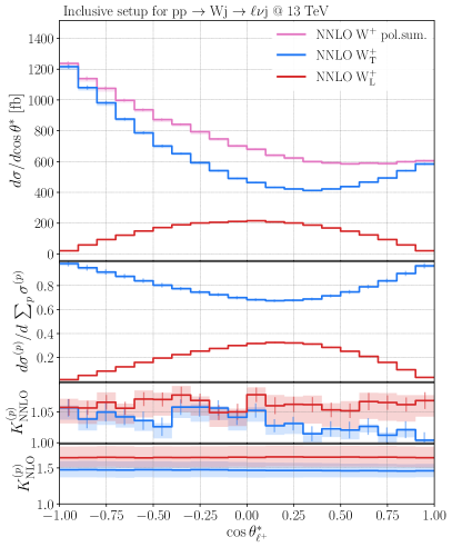
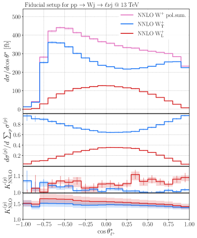
Figure 2: Differential distributions for $\cos\theta^{*}_{\ell^{+}}$ in the inclusive (left) and fiducial (right) setup for $\text{p}\text{p}\rightarrow\ell^{+}\,\nu_{\ell}\text{j}$ process. In the upper pane, the transverse and longitudinal polarised predictions as well as their sum are displayed at NNLO QCD accuracy. In the middle pane, the transverse and longitudinal polarised predictions are normalised to the sum of the two. The lower pane shows the respective $K$-factors (NLO and NNLO) for the various polarised predictions. The bands represent the 7-point scale variation while the bars indicate the Monte Carlo uncertainty.

We obtain polarisation fractions as a fraction of each polarised cross section to the overall sum for each setup. Another method to obtain fractions would be a convolution with Legendre polynomials Ballestrero:2017bxn in the Monte Carlo integration of an unpolarised setup. However, it is only applicable in the absence of leptonic phase space cuts, as it relies on the analytic expression of the cross section as a function of the leptonic emission polar angle Bern:2011ie ; Stirling:2013muo . We checked that in the inclusive setup the result of this method coincides within statistical uncertainties with the last column of table 1.

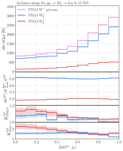
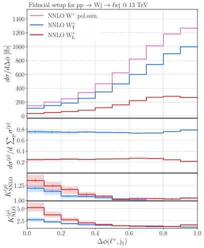
Figure 3: Differential distributions for $\Delta\phi(\ell^{+},\text{j}_{1})$. Same plot structure as in figure 2.

Another question is the estimation of theoretical uncertainty for the polarisation fractions. It was first addressed in ref. Bern:2011ie , where the authors encountered very low sensitivity of the polarisation fractions to the variation of the scale and resorted to comparing parton-shower and fixed-order predictions to estimate the uncertainty. We believe this would be the best strategy for NLO precision. However, with NNLO corrections at hand, we decided to estimate the scale uncertainty by varying the fixed-order prediction scale in an uncorrelated way, meaning that errors in the ratio are propagated via the usual chain rule.

The effect that clearly stands out is that longitudinal polarisation receives a larger correction than the transverse one in all setups. It is not surprising and applies to various other processes Poncelet:2021jmj ; Denner:2020bcz . This is even more apparent on several differential distributions in figures 2-5, where the plots on the left- and right-hand side represent the inclusive and fiducial setup, respectively. We only show results for the “plus” signature here.

The main observable for vector-boson polarisation is the polar-angle distribution of the leptonic emission, presented in figure 2. In the inclusive setup the longitudinal mode is perfectly symmetric in the angle of emission; the transverse mode dominates and peaks for the case of backwards emission, as a consequence of W-bosons being created left-handed at the LHC Bern:2011ie . Fiducial cuts significantly change the shape of the absolute distributions. However, this does not have a large effect on the distributions of the fractions. Due to their distinct profiles, these shapes would allow for the most efficient separation of polarisations via shape fitting, but alas, the neutrino momentum is not available experimentally to fully reconstruct the angle of leptonic emission. Therefore, experiments have utilised available transverse momenta to have a handle on the emission angle. These are $\cos\theta^{*}_{\text{2D}}$ for ATLAS ATLAS:2012au and $L_{P}$ for CMS CMS:2011kaj . Naturally, the difference in shapes between polarisations is partially washed out in comparison with the actual polar-angle distribution.

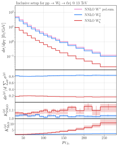
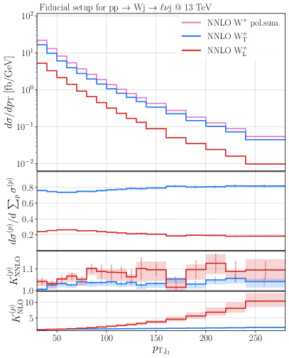
Figure 4: Differential distributions for $p_{{\mathrm{T}},\text{j}_{1}}$. Same plot structure as in figure 2.

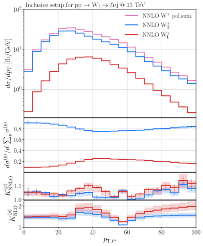
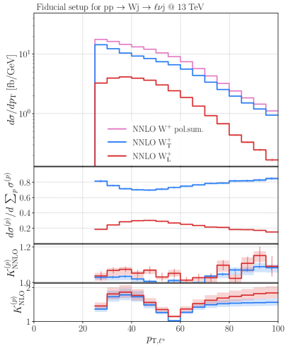
Figure 5: Differential distributions for $p_{\rm T,\ell^{+}}$. Same plot structure as in figure 2.

An angular observable that is readily available at the experimental level is for example, the azimuthal angle between the charged lepton and the hardest jet ($\text{j}_{1}$), presented in figure 3. This observable was measured, for example, by the CMS experiment in ref. CMS:2017gbl . The corrections at NLO are different between the longitudinal and transverse polarisations but are quite similar at NNLO. Fiducial cuts significantly raise the QCD corrections at lower angles.

QCD corrections are particularly important in energy related distributions. In figure 4 we display transverse momentum of the hardest jet. The NLO corrections are rising seemingly without a bound for the longitudinal component. At NNLO, the corrections are stable, oscillating around 10%, showing a good sign for the perturbative convergence. Similar giant $K$-factor at NLO appear in other energy-related distributions involving jets: $H_{\mathrm{T}}$, invariant masses, other $p_{\mathrm{T}}$ distributions.

In the context of shape fits, we would like to discuss the observable for the transverse momentum of the charged lepton in figure 5, although similar features are naturally present in the missing $p_{\mathrm{T}}$ distribution. It has a remarkably distinct shape of polarisation fraction profile, which is useful for shape fitting. The NLO corrections are typically large at high $p_{\mathrm{T}}$ but seem to flatten out in contrast to the case of jet $p_{\mathrm{T}}$ highlighted above. The shapes of corrections seem similar otherwise. The longitudinal polarisation receives stronger corrections near the peak, reflecting the fact that at the level of total cross section the $K$-factors are larger.

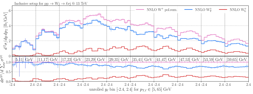
Figure 6: Double differential distributions for $\text{p}\text{p}\rightarrow\ell^{+}\,\nu_{\ell}\text{j}$ in the inclusive setup in the $p_{\rm T,\ell^{+}}$ and $y_{\ell^{+}}$ observables. In the upper plot, the transverse and longitudinal polarised predictions as well as their sum are displayed at NNLO QCD accuracy. In the lower pane, the transverse and longitudinal polarised predictions are normalised to the sum of the two. The bands represent the 7-point scale variation while the bars indicate the Monte Carlo uncertainty.

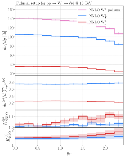
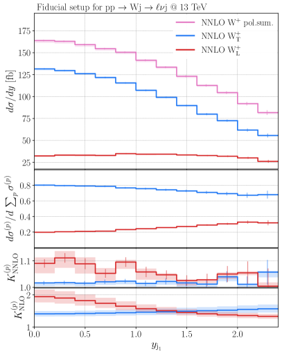
Figure 7: Differential distributions for symmetrised $y_{\ell^{+}}$ (left) and $y_{\text{j}_{1}}$ (right), both in the fiducial setup. Individual plots follow the structure of figure 2.

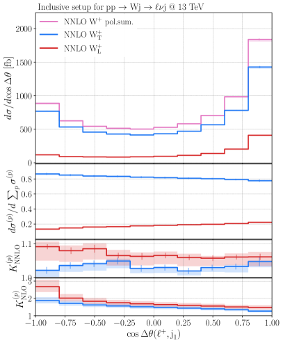
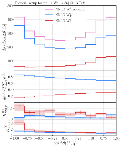
Figure 8: Differential distributions for symmetrised $\cos\theta(\ell^{+},\text{j}_{1})$ in the inclusive (left) and fiducial (right) setups. Individual plots follow the structure of figure 2.

In figure 6, we show the double differential distribution in the transverse momentum and the rapidity of the charged lepton. Such a 2D information can also be particularly useful for the extraction of polarisation fractions through fitting as they provide complementary information. This kind of measurements have been already presented in ref. CMS:2020cph for the Drell-Yan process. In the present case, the transverse momentum and the rapidity of the charged lepton constitute a very good combination as they are not correlated. The 2D distribution features a change of rapidity profiles for different transverse momentum bins. Interestingly, the ordinary 1D lepton rapidity distribution shows almost completely flat polarisation fraction profile. One can observe that the longitudinal polarisation is at maximum for transverse momentum around $50\,\text{GeV}$ and central rapidity. An experimental $\text{W}\!+\text{j}$ analysis based on 2D information would be therefore highly valuable and very complementary to the one for the Drell-Yan process.

A possibly even more sensitive observable in combination with lepton $p_{\mathrm{T}}$ would make the jet rapidity, which we compare separately to lepton rapidity in figure 7. Jet rapidity seems to have more pronounced monotonically decreasing polarisations shapes at lower rapidities $\absolutevalue{y}<1.7$ — which is the area where off-shell and interference effects are low, as is shown further in section 3.3. Similarly to lepton rapidity, jet rapidity is (to a large extent) independent of lepton $p_{\mathrm{T}}$, and thus if one wants to make a more constraining fit, the possible alternative would be to use a 2D distribution of jet rapidity and lepton $p_{\mathrm{T}}$, which will one could in principle fit all polarisations and signatures independently at once.

Finally, we show another observable in figure 8 which we believe would be helpful in experimental analyses: the angle between the charged lepton and the hardest jet. The difference between polarisation shapes is by a factor of 2 more pronounced in the fiducial setup, which makes it very useful in extracting polarisations using the method of shape fitting. The NNLO corrections for both polarisations are mild and flat.

3.2 Charge differences

The two signatures of the $\text{p}\text{p}\rightarrow\ell^{\pm}\,\overset{\scriptscriptstyle(-)}{\nu}_{\!\!\!\ell}\,\text{j}$ process behave differently, and there are two distinctive reasons within the SM for that: differences in the lepton emission distribution, and the PDFs of the initial-state partons.

The first effect is evident from the distribution of the polar emission angle of the charged lepton in figure 9. In the inclusive setup, the shapes look almost mirrored, and peak in opposite the regions: at $-1$ for the “plus” signature, and at $+1$ for the “minus” one. In fact, these shapes can be described analytically, as long as no leptonic cuts are imposed Bern:2011ie . The shapes change dramatically on the edges in the fiducial setup due the kinematic constrains on the lepton. It is interesting to notice that the ratio of the polarisation fraction of the two signatures shows a perfect oscillatory behaviour that can be traced back to their analytical expressions and is thus independent of the setup. Also, it is worth mentioning that such ratios (see also figures 11 and 11) show essentially no shape distortion with respect to higher-order corrections, making them particularly attractive for experimental studies.

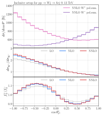
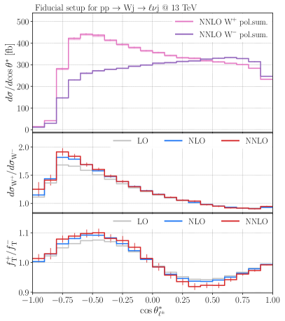
Figure 9: Differential distributions of $\cos\theta^{*}_{\ell^{\pm}}$ for $\text{p}\text{p}\rightarrow\ell^{\pm}\,\overset{\scriptscriptstyle(-)}{\nu}_{\!\!\!\ell}\,\text{j}$ in the inclusive (left) and fiducial (right) setup. In the upper pane, the sum of the transversely and longitudinally polarised predictions for both signatures are displayed at NNLO QCD accuracy. In the middle pane, the ratio of the two signatures is shown at LO, NLO, and NNLO. The lower pane presents the ratio of the differential distributions of transverse polarisation fractions between the two signatures, also at LO, NLO, and NNLO. In the upper plot, the bands represent the 7-point scale variation, while the bars indicate the Monte Carlo uncertainty for in all three plots.

The direction of emission angle is directly connected to the transverse momentum of the lepton, displayed in figure 11. We observe a constant behaviour except in the region $25<p_{{\mathrm{T}},\ell}<60\,\text{GeV}$, where “minus” signature has a much flatter behaviour and catches up with “plus” signature at the beginning of the tail. As the emission angle distribution shows, the lepton of the “minus” signature tends to be emitted in the direction of the W-boson, thus making it more likely to have higher $p_{\mathrm{T}}$. Fiducial cuts do not affect these conclusions, except that there are no events below the leptonic cut. This observable also has an excellent capability to discern not only polarisations but also the particular process signature.

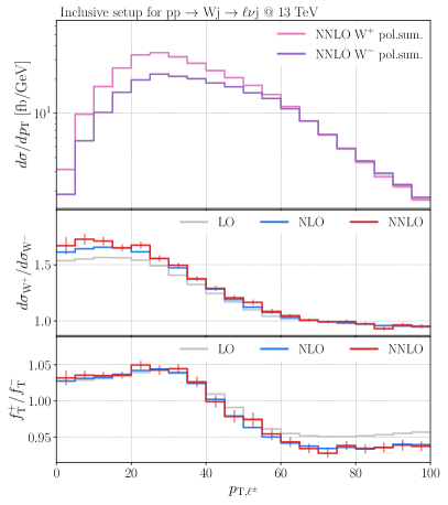
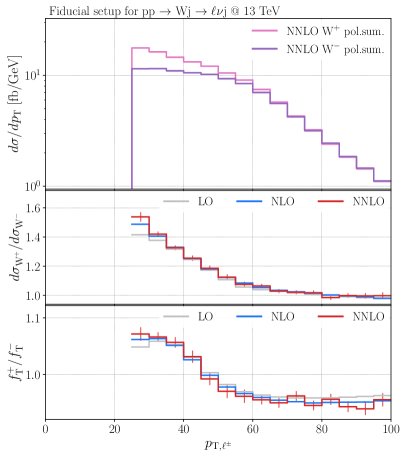
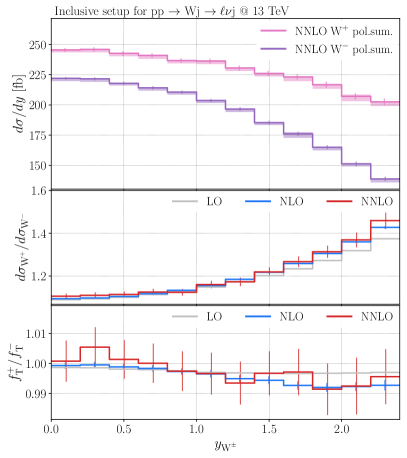
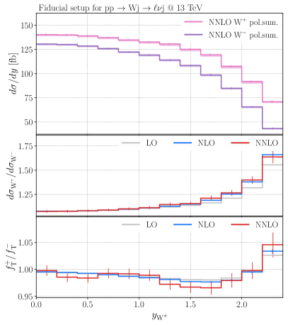
Figure 10: Differential distributions of $p_{{\mathrm{T}}}(\ell)$ for $\text{p}\text{p}\rightarrow\ell^{\pm}\,\overset{\scriptscriptstyle(-)}{\nu}_{\!\!\!\ell}\,\text{j}$ in the inclusive (left) and fiducial (right) setup. same individual plot structure as in figure 9.

Figure 11: Differential distributions of $y_{\text{W}}$ for $\text{p}\text{p}\rightarrow\ell^{\pm}\,\overset{\scriptscriptstyle(-)}{\nu}_{\!\!\!\ell}\,\text{j}$ in the inclusive (left) and fiducial (right) setup. Same individual plot structure as in figure 9.

The other effect is due to differences in PDFs for the initial-state partons. As was noted previously, the “plus” signature has a larger cross-section due to the dominance of ug-channel over dg-channel. The distribution of W-boson rapidity in figure 11 also looks much more spread out for the “plus” signature. The same effect is present, although in a more suppressed form, in $y_{\ell}$ and $y_{\text{j}_{1}}$. As for the ratio of transverse polarisation fractions, one can see that this observable is not sensitive to left-right asymmetry of W-bosons.

3.3 Off-shell, interference effects, and comparison with data

So far, the discussion focused on polarised predictions. Nonetheless, such predictions are only approximations to the full off-shell and unpolarised process. In this section we address limitations of the NWA polarised computation by comparing it to unpolarised predictions (within the NWA framework) as well as to the fully off-shell calculation. We also compare simulations with the available data from the CMS collaboration CMS:2017gbl .

We start by comparing unpolarised predictions to the sum of the polarised ones in the inclusive setup in table 3. The difference between the two constitutes an estimate of the interference effects between the polarisation states. Interference effects appear to be consistent with zero within the Monte Carlo uncertainty for all perturbative orders and for both signatures.

Inclusive	LO [fb]	NLO [fb]	$K_{\text{NLO}}$	NNLO [fb]	$K_{\text{NNLO}}$
$\text{W}^{+}_{\text{unpol.\ }}$	$990.00(8)^{+11.5\%}_{-9.3\%}$	$1483.1(5)^{+7.9\%}_{-7.0\%}$	$1.50$	$1541(5)^{+0.5\%}_{-1.9\%}$	$1.04$
$\text{W}^{+}$ pol. sum.	$989.97(7)^{+11.5\%}_{-9.3\%}$	$1482.8(5)^{+7.9\%}_{-7.0\%}$	$1.50$	$1546(6)^{+0.3\%}_{-1.9\%}$	$1.04$
$\text{W}^{-}_{\text{unpol.\ }}$	$774.04(6)^{+11.5\%}_{-9.3\%}$	$1121.1(3)^{+7.1\%}_{-6.5\%}$	$1.45$	$1158(4)^{+0.3\%}_{-1.7\%}$	$1.03$
$\text{W}^{-}$ pol. sum.	$773.97(5)^{+11.5\%}_{-9.3\%}$	$1121.2(3)^{+7.1\%}_{-6.5\%}$	$1.45$	$1155(3)^{+0.2\%}_{-1.5\%}$	$1.03$

Table 3: Total cross sections of $\text{p}\text{p}\rightarrow\ell^{\pm}\,\overset{\scriptscriptstyle(-)}{\nu}_{\!\!\!\ell}\,\text{j}$ for the inclusive setup at the LHC with the centre-of-mass energy of $\sqrt{s}=13\,\text{TeV}$. The unpolarised and polarised-sum predictions are provided at LO, NLO, and NNLO accuracy along with the corresponding $K$-factors. Numbers in parentheses indicate statistical errors while sub- and superscripts represent scale uncertainty.

Similarly, we provide predictions for the fiducial setup in table 4, where we also compare to off-shell results. The difference between the unpolarised and the sum of polarised results indicates negligible (per mille) interference effects. The difference to off-shell computation however is much more significant and presents a 1-2% effect. This is in agreement with the naive estimate $\mathcal{O}{\left(\Gamma_{\text{W}}/M_{\text{W}}\right)}$ for the accuracy of the NWA. We note that these differences are purely due to off-shell effects and do not involve any missing non-resonant diagrams in the NWA calculation, which is the case for other processes involving neutral currents. Off-shell effects persist throughout QCD corrections as they are only concerned with the production part of the amplitude, whereas the decay part is purely an EW process.

Fiducial	LO [fb]	NLO [fb]	$K_{\text{NLO}}$	NNLO [fb]	$K_{\text{NNLO}}$
$\text{W}^{+}$ off-shell	$408.69(3)^{+11.5\%}_{-9.3\%}$	$607.7(4)^{+7.1\%}_{-6.5\%}$	$1.49$	$626(3)^{+0.2\%}_{-1.6\%}$	$1.03$
$\text{W}^{+}_{\text{unpol.\ }}$	$413.83(2)^{+11.5\%}_{-9.3\%}$	$615.7(2)^{+7.1\%}_{-6.5\%}$	$1.49$	$635(2)^{+0.2\%}_{-1.6\%}$	$1.03$
$\text{W}^{+}$ pol. sum.	$413.21(3)^{+11.5\%}_{-9.3\%}$	$613.6(2)^{+7.1\%}_{-6.5\%}$	$1.49$	$633(2)^{+0.2\%}_{-1.6\%}$	$1.03$
$\text{W}^{-}$ off-shell	$347.19(2)^{+11.5\%}_{-9.3\%}$	$504.8(1)^{+6.6\%}_{-6.1\%}$	$1.45$	$518(2)^{+0.3\%}_{-1.3\%}$	$1.03$
$\text{W}^{-}_{\text{unpol.\ }}$	$352.94(2)^{+11.5\%}_{-9.3\%}$	$513.7(1)^{+6.6\%}_{-6.2\%}$	$1.46$	$528(2)^{+0.2\%}_{-1.5\%}$	$1.03$
$\text{W}^{-}$ pol. sum.	$352.91(2)^{+11.5\%}_{-9.3\%}$	$512.3(1)^{+6.6\%}_{-6.2\%}$	$1.45$	$525(1)^{+0.2\%}_{-1.3\%}$	$1.03$

Table 4: Total cross sections of $\text{p}\text{p}\rightarrow\ell^{\pm}\,\overset{\scriptscriptstyle(-)}{\nu}_{\!\!\!\ell}\,\text{j}$ for the fiducial setup at the LHC with a centre of mass of $\sqrt{s}=13\,\text{TeV}$. The unpolarised and polarised-sum predictions are provided at LO, NLO, and NNLO accuracy as well as with the corresponding $K$-factors. All cross sections are expressed in  fb. The numbers in parenthesis indicate the numerical error while the ones in per cent represent 7-scale variation.

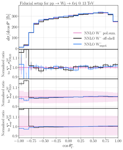
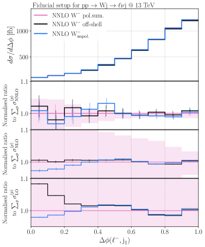
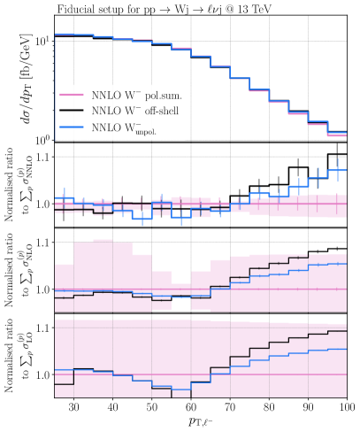
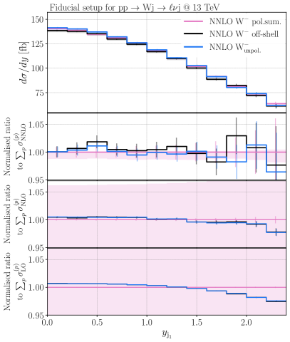
Figure 12: Differential distributions for $\text{p}\text{p}\rightarrow\ell^{-}\,\bar{\nu}_{\ell}\text{j}$ in the fiducial setup: $\cos\theta^{*}_{\ell^{-}}$ (top left), $\Delta\phi(\ell^{-},\text{j}_{1})$ (top right), $p_{\rm\text{W}^{-}}$ (bottom left), and $p_{\rm\ell^{-}}$ (bottom right). The upper pane shows absolute distributions at NNLO QCD in the following setups: unpolarised NWA, the sum of polarised NWA, and off-shell. The other three panes feature the same distributions normalised to the sum of polarised setups at LO, NLO and NNLO. The pink band represents the 7-point scale variation for the ratio denominator, while the bars indicate the Monte Carlo uncertainty.

We turn to differential distributions presented in figure 12. Starting with the $\cos\theta^{*}_{\ell^{-}}$ observable, one can see the off-shell and polarisation interference effects consistent with zero, apart from the low angles, where $\cos\theta^{*}_{\ell}<-0.75$. This region corresponds to the backwards emission of the charged lepton, and it is heavily influenced by the phase-space cuts. Given the distinct polarisation shapes as presented in figure 2 and the absence of approximation effects elsewhere, this observable would be perfectly suited to separate polarisations. However, neutrino momentum is not fully available at experiments, so proxies such as $L_{P}$ or $\cos\theta_{\text{2D}}$ are used.

Looking at the distribution of the azimuthal angle between the charged lepton and the jet, we see the appearance of some non-trivial interference and off-shell effects. Interference effects can appear only when the angular integration is restricted, which is what happens with this observable due to its definition. The effects are still within scale uncertainty at NNLO. Note how the off-shell effects reach almost 10% at LO at lower angles and vanish at NLO. This part of the phase space at LO corresponds to the charged lepton and the jet both recoiling against the neutrino — an unlikely event, with a higher probability for off-shell W-bosons. At NLO, due to real radiation, such a topology is no more suppressed, and thus, this part of the phase space receives a significant correction which washes out the off-shell effects at lower order.

Next, we discuss the transverse momentum of the charged lepton. The plot shows that at $25<p_{\mathrm{T}}<70\,\text{GeV}$ interference and off-shell effects are rather low, under 3%, and afterwards start to rise up to 10% for off-shell and 5% for interference effects, peaking at $p_{{\mathrm{T}},\ell}=110\,\text{GeV}$. Given that the longitudinal polarisation fraction falls off rapidly at higher energies, we do not investigate the high-energy region. One can see that the magnitude of the approximation effects drops down for NLO corrections and is consistent with its level at NNLO. In conjunction with the distinct polarisation-shape profile, this observable is well suited for polarisation studies in the specified region. The same conclusions apply to the other process signature.

Having investigated both off-shell and interference effects differentially, we can put them in perspective with experimental data. Such an analysis for several differential distributions is presented in figure 13. Specifically, the sum of polarised predictions and the off-shell calculation are compared against data for the combined signatures of the W+j process.

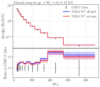
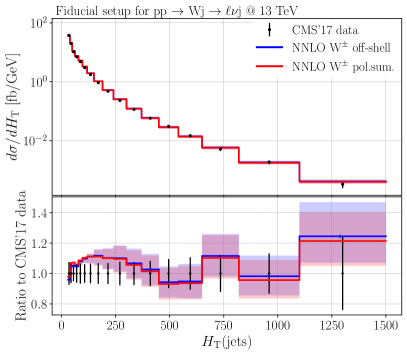
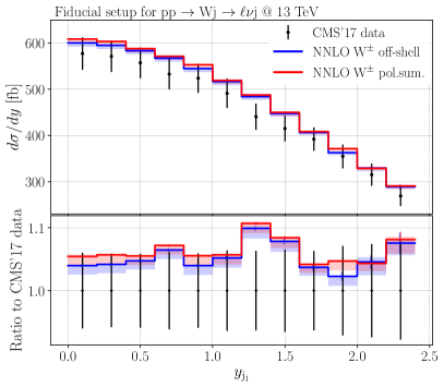
Figure 13: Differential distributions for $\text{p}\text{p}\rightarrow\ell^{\pm}\,\overset{\scriptscriptstyle(-)}{\nu}_{\!\!\!\ell}\,\text{j}$ in the fiducial setup: transverse momentum of the hardest jet (top left), transverse energy of jets (top right), azimuthal angle between the charged lepton and the hardest jet (bottom left), and rapidity of the hardest jet (bottom right). The upper pane features absolute predictions at NNLO for the polarised sum in the NWA and the off-shell setup. The data points are taken from ref. CMS:2017gbl . The lower pane shows the same predictions normalised to the experimental data. The bands represent scale variation uncertainty.

In general the agreement is rather good: the data and the theoretical predictions agree within uncertainties. However, the NNLO-precise calculations tend to overshoot the data, both at the level of differential distributions and total cross section. Missing EW corrections can potentially account for this effect. They are expected to be negative and have a magnitude of 5-20% depending on the energy scale Denner:2009gj . In addition, the data were originally compared with another NNLO calculation presented in ref. CMS:2017gbl , and as an important cross check, we observed that in all presented distributions, our results are in agreement at the per-cent level with the exception of $\Delta\phi(\ell^{\pm},\text{j}_{1})$ at smaller angles, where our result gets to about one scale band lower (roughly $10\%$), while still being in agreement with experimental data. This mismatch originates from the different scale choice. In ref. Boughezal:2016dtm , the central scale is $\mu=\sqrt{M^{2}_{\ell\nu}+\sum_{i}p^{2}_{\rm T,\text{j}_{i}}}$. It coincides with our definition in eq. (12) asymptotically at high $p_{\mathrm{T}}$, but behaves differently at low $p_{\mathrm{T}}$. The small angle between the jet and the charged lepton corresponds to the smaller energies, hence the difference between the two NNLO calculations.

We would like to stress that the shortcomings of the polarised NWA predictions are negligible in comparison to experimental uncertainties and are mostly within estimated missing higher-order contributions. This gives reassurance that boson polarisation studies are well justified for W+j process and would benefit from more precise experimental measurements.

3.4 Fitting polarised fractions

In section 2.1 we discussed how to extract longitudinal and transverse boson polarisations. Polarisation fractions are simply theoretical quantities that depend on the intricate structure of the EW sector in the particle theory of the nature. It means that such parameters can only be experimentally extracted in an indirect way, based on theoretical inputs. One of the commonly used methods is template fitting. It prescribes fitting predefined shapes of polarised (theoretical) predictions to the data. In this section we will show how such method benefits from NNLO-accurate predictions.

As a first step towards experimental application, we use mock data for which we simply take the NNLO fully off-shell prediction. The underlying assumption is that these distributions are best suited to describe the data and can therefore serve as a proxy for a more precise experimental measurement. In particular, the mock data errors are generated according to the NNLO fully off-shell prediction based on a total luminosity of 250 fb^-1. The fit only considers bins where the off-shell and interference effects are small: in particular, we use a 3% criterion. The polarisation fractions are fitted as linear coefficients that multiply the normalised polarisation shapes. The more distinct the shapes are, the more precise the fit will be. We have also checked that fits to unpolarised and sum of polarised setups produce similar results.

Both polarisations are fitted independently using a $\chi^{2}$ fit for each of the 7 scales taking into account all errors:

$$\chi^{2}=\sum\limits_{i\in\text{bins}}\frac{\left(\sigma^{i}_{\text{off-shell}}-\sum\limits_{j=\text{L,T}}\alpha_{j}\cdot\sigma^{i}_{\text{pol},j}\right)^{2}}{(\epsilon^{i}_{\text{off-shell}})^{2}+\sum\limits_{j=\text{L,T}}(\alpha_{j}\cdot\epsilon^{i}_{\text{pol},j})^{2}},$$ (17)

where $\varepsilon^{i}_{\text{off-shell}}=\sqrt{\sigma^{i}_{\text{off-shell}}/L}$ is the luminosity-projected error on the off-shell differential distribution, $\varepsilon^{i}_{\text{pol},j}$ are the Monte-Carlo errors of the polarised calculation $j$, and $\alpha_{j}$ are the fitting coefficients. We also combine distributions of both signatures, treating polarisation fractions as charge-independent. This choice is based on the extreme proximity of the corresponding fractions in table 2. For each of the scale choices, we obtain $1\sigma$ and $2\sigma$ confidence regions in the $f_{\text{L}}-f_{\text{T}}$ plane. The envelop of all such regions then serves as a proxy for theoretical uncertainty of the result. NLO and NNLO predictions differ not only in the size of the scale uncertainty, but also in the variation of the normalised distribution shapes, which affects the spread of fits at different scale choices. To compare the two, we present fits performed using NLO predictions on the left and NNLO predictions on the right. The $1\sigma$ and $2\sigma$ confidence regions maintain their form which is defined by the errors of the data that is being fit, but the spread of the fits changes. To show how the result of the fit compares with our results from polarised cross section calculations, we present the error bar corresponding to polarisation fractions in table 2 and its theoretical uncertainty.

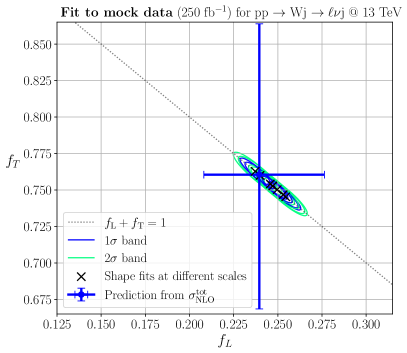
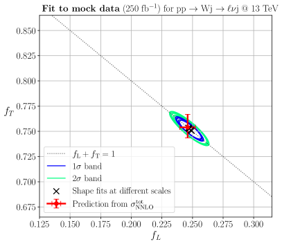
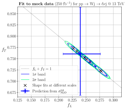
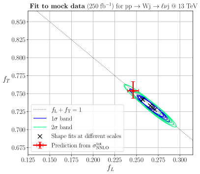
Figure 14: Fit to the mock data of the polarisation fractions for both signatures $\text{p}\text{p}\rightarrow\ell^{\pm}\,\overset{\scriptscriptstyle(-)}{\nu}_{\!\!\!\ell}\,\text{j}$ in the fiducial setup using polar angle of the charged lepton emission at NLO (left) and NNLO (right). The blue and light green contours identify $1\sigma$ and $2\sigma$ regions, respectively. Each ellipsis in the $f_{\rm T}$ and $f_{\rm T}$ plane corresponds to the uncertainty of the fit of one setup in the 7-scale set. The error bar represents the prediction for the polarisation fractions from table 2.

Figure 15: Fit to the mock data of the polarisation fractions for both signatures $\text{p}\text{p}\rightarrow\ell^{\pm}\,\overset{\scriptscriptstyle(-)}{\nu}_{\!\!\!\ell}\,\text{j}$ in the fiducial setup using polar angle between the charged lepton and the hardest jet at NLO (left) and NNLO (right). Same plot structure as in figure 15.

The fit using the polar emission angle of the charged lepton is presented in figure 15. The uncertainty on the longitudinal fraction estimated from the fit shrinks by 50% at NNLO and is determined by the size of the ellipse, while the shape variation is drastically reduced. This observable has the highest power to discern polarisations and thus yields the lowest uncertainty. As we observed, the shape variation is generally greatly reduced at NNLO, in comparison to NLO, but interestingly, the LO shape variation is also very small. Its fit, however, would be completely meaningless given the large $K$-factors.

Next, we present another observable which is rather sensitive to polarisation fractions: the polar angle between the charged lepton and the hardest jet in figure 15. The spread is greatly reduced but not quite as fully as in the previous case. With data uncertainties taken into account, NNLO corrections reduce the size of the overall envelope uncertainty by 50%. This is an excellent observable which could be used in experimental analyses.

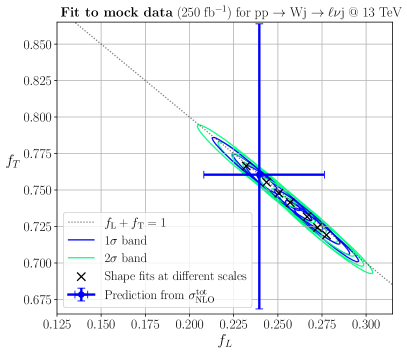
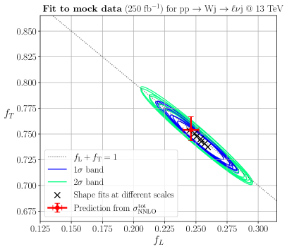
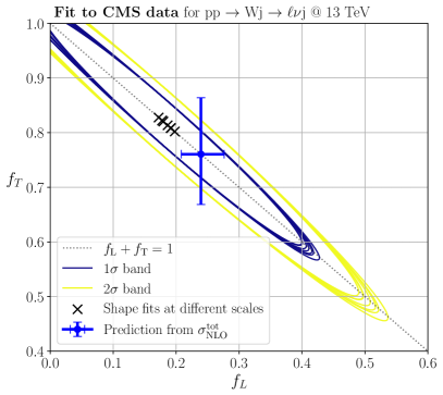
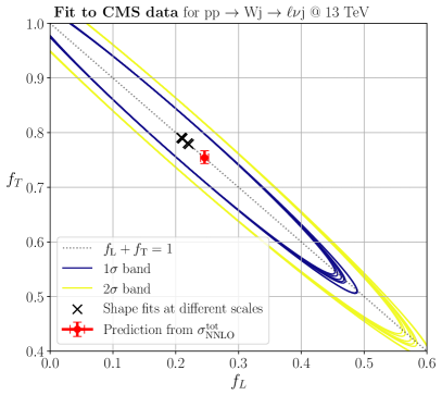
Figure 16: Fit to the mock data of the polarisation fractions for both signatures of $\text{p}\text{p}\rightarrow\ell^{\pm}\,\overset{\scriptscriptstyle(-)}{\nu}_{\!\!\!\ell}\,\text{j}$ in the fiducial setup using the 2D distribution of rapidity and transverse momentum of the charged lepton at NLO (left) and NNLO (right). Same plot structure as in figure 15.

Figure 17: Fit to the CMS data CMS:2017gbl of the polarisation fractions for both signatures $\text{p}\text{p}\rightarrow\ell^{\pm}\,\overset{\scriptscriptstyle(-)}{\nu}_{\!\!\!\ell}\,\text{j}$ in the fiducial setup using the $y_{\text{j}_{1}}$ distribution at NLO (left) and NNLO (right). Experimental systematic errors were separated from statistical errors. Statistical errors were further decreased by a factor of 3. Same plot structure as in figure 15, except for the $2\sigma$ band which is displayed in yellow.

In figure 17, we fit to the two-dimensional distribution of the transverse momentum and rapidity of the charged lepton. After reducing the data set in the transverse-momentum observable to minimise off-shell and interference effects, this observable possesses a strong discrimination power. As mentioned previously, we expect that the pair of $y_{\text{j}_{1}}$ and the lepton $p_{\text{T}}$ will have similar or even stronger polarisation separation power, since in contrast to lepton rapidity, jet rapidity is sensitive to polarisation shapes. Still, the evolution of $y_{\ell}$ shape at different energies seems to be non-trivial enough to help the presented 2D distribution to perform better than $p_{\text{T},\ell}$ alone.

Finally, in figure 17, we exercise a fit to the experimental data in ref. CMS:2017gbl . Out of the presented observables, we picked $y_{\text{j}_{1}}$ as it provides the strongest sensitivity to polarisations. Unfortunately, the size of the error bars in ref.CMS:2017gbl , which are based on the measurement with a total luminosity of 2.2 fb^-1, does not allow for a sensible fit, suggesting that the longitudinal polarisation fraction is anywhere in the interval $[0,0.5]$. This accuracy is expected to significantly improve with larger statistics during the high-luminosity phase of the LHC Azzi:2019yne and resemble the results obtained in our mock data fit shown above.

The presented examples here aim at illustrating the role of NNLO corrections in the polarisation studies. There are many other observables that could be helpful in discerning polarisations, e.g. $\Delta R$, $L_{p}$, $\cos\theta^{*}_{\text{2D}}$; but as a rule the fitting results are universally improved, due to the reduction in shape variation at NNLO. Combination of independent observables might also improve the fitting procedure as they can provide extra (independent) information.

To conclude, we would like to emphasise that we have presented all theoretical ingredients needed for the experimental extraction of polarised fractions. A detailed analysis of how the fits should be done and how results should be presented is left for future work. In particular, there is still a number of open questions. Should the two signatures be fitted separately or together? How should theoretical uncertainties be taken into account in the fit? How should one define the overall uncertainty on the fit of the polarisation fractions? We believe that these questions should be addressed in collaboration with experimental groups.

4 Conclusion

The exploration of the intricate structure of the EW sector in the SM is one of the most exciting aspects of the LHC physics. One way of probing it is through the extraction of polarisation fractions, which are thought to be sensitive to potential new-physics effects. This article builds upon this idea by presenting, for the first time, predictions for the polarised production of W+j at the LHC up to NNLO QCD accuracy in the SM.

In particular, we have studied in detail the behaviour of the transverse and longitudinal parts in two setups: inclusive and fiducial. The first one contains only some jet requirements, whereas the second one reproduces the event selection of the CMS measurement CMS:2017gbl at $13\,\text{TeV}$. Application of cuts has a large impact on the polarisation fraction meaning that a lot of care needs to be taken when extrapolating results from a fiducial volume to the inclusive phase space. Also, similarly to what was shown in other processes, different polarised processes receive different QCD corrections up to NNLO accuracy. This advocates for the use of tailored predictions in experimental analysis.

As the usage of polarised prediction relies on a number of approximations, we have investigated their effects in detail. In particular, we studied off-shell effects arising due to NWA and interferences between polarisation states. Compared to missing higher-orders estimated through scale variation, such effects are rather suppressed. In the same way, the experimental uncertainties are significantly larger than the shifts induced by such approximations. Overall, we conclude that for $\text{W}^{\pm}\text{j}$ production at the LHC, the use of polarised predictions within the NWA is without a doubt a very good approximation of the full process.

Finally, we have performed global fits of the polarisation fractions using mock data (the off-shell computations) as well as experimental data. By doing so, we have singled out the most sensitive observables for the determination of polarisation fractions. Also, we have shown that with sufficiently precise data, using NNLO predictions allows for a more precise determination of polarisation fractions than with lower-order predictions.

In the present work, we have presented all theoretical ingredients necessary for the experimental extraction of polarisation fractions at the LHC. In particular, we will happy to provide all theoretical predictions (cross sections and differential distributions) in data format upon request. These could be used right away by experimental collaboration to extract polarisation fractions with existing data, hence paving the way for the precise exploration of the EW sector of the SM in the high-luminosity phase of the LHC.

Appendix A Polarised two-loop matrix elements

The two-loop amplitudes for the partonic process

$$\bar{q}^{\prime}q\to\text{W}\text{g},$$ (18)

and the corresponding crossed ones, are a necessary input for the NNLO QCD corrections to the polarised cross sections. The amplitudes for the off-shell process, including the leptonic decay of the W-boson, have been presented in ref. Gehrmann:2011ab . We use their notation in what follows. The essential result of this work is the independent helicity structure coefficients $\alpha$, $\beta$, and $\gamma$ — also published explicitly up to two-loop order. The amplitude $\mathcal{M}(\bar{q}^{\prime}q\to\text{W}\text{g})$ can be written in terms of the partonic current $S^{\mu}$ and the polarisation vector $\epsilon_{\mu}$ of the W-boson:

$$\mathcal{M}(q,h)=\epsilon_{\mu}(q,h)S^{\mu}\;,$$ (19)

where the dependence on the W-boson momentum and polarisation $h$ has been made explicit. Furthermore, the right-handed partonic current $S^{\mu}_{R}$ can be decomposed into helicity structures as follows:

$$S_{R}^{\mu} (p_{1}^{-};p_{3}^{+};p_{2}^{+})=\frac{1}{\sqrt{2}}\langle 12\rangle[13]^{2}\left(p_{1\mu}A_{11}+p_{2\mu}A_{12}+p_{3\mu}A_{13}\right)-\frac{1}{\sqrt{2}}\frac{\langle 12\rangle[13]}{\langle 23\rangle}[1\;|\gamma_{\mu}|\;2\rangle\;s_{23}B$$

$$+\frac{1}{\sqrt{2}}[13][3\;|\gamma_{\mu}|\;2\rangle\;\left[s_{23}B+\frac{1}{2}\left((A_{11}+A_{12})s_{12}+(A_{11}+A_{13})s_{13}+(A_{12}+A_{13})s_{23}\right)\right],$$ (20)

featuring the scalar coefficients $A_{11}$, $A_{12}$, $A_{13}$, and $B$. After contraction with the decay current, only three linear combinations of these coefficients ($A_{11}$, $A_{12}+2B$, and $A_{13}$) remain. These combinations are linearly related to the already mentioned coefficients $\alpha$, $\beta$, and $\gamma$, but it worth mentioning that the $A_{1j}$ and $B$ coefficients cannot be obtained separately from $\alpha$, $\beta$, and $\gamma$. Due to transversality of the polarisation vector $\varepsilon_{\mu}$, one expects that this reduction of linear independent coefficients occurs in the same way for the on-shell amplitude as well. The purpose of the rest of this note is to explicitly show this property.

We start by decomposing the polarisation vector in terms of a momentum basis which spans the four dimensional space:

$$\epsilon^{\mu}=c_{1}p_{1}^{\mu}+c_{2}p_{2}^{\mu}+c_{3}p_{3}^{\mu}+c_{4}\epsilon^{\mu}_{p_{1},p_{2},p_{3}}/s_{12}\,,$$ (21)

where $\epsilon^{\mu}_{p_{1},p_{2},p_{3}}=\epsilon^{\mu\nu\rho\sigma}p_{1,\nu}p_{2,\rho}p_{3,\sigma}$ is the contracted Levi-Civita symbol and $c_{i}$ are scalar coefficients. With the usage of the standard spinor-helicity identities, the contraction of $S^{\mu}_{R}$ with the external momenta $p_{1},p_{2},p_{3}$ and $\epsilon_{p_{1},p_{2},p_{3}}$ leads to

$$S^{p_{1}}_{R}=p_{1\mu}S^{\mu}_{R}= -\frac{\langle 12\rangle[13]^{2}}{2\sqrt{2}}\bigl{(}A_{11}(s_{12}+s_{13})+A_{13}s_{23}+(A_{12}+2B)s_{23}\bigr{)},$$ (22)

$$S^{p_{2}}_{R}=p_{2\mu}S^{\mu}_{R}= \frac{\langle 12\rangle[13]^{2}}{2\sqrt{2}}\bigl{(}A_{11}s_{12}+A_{13}s_{23}\bigr{)},$$ (23)

$$S^{p_{3}}_{R}=p_{3\mu}S^{\mu}_{R}= \frac{\langle 12\rangle[13]^{2}}{2\sqrt{2}}\bigl{(}A_{11}s_{13}+(A_{12}+2B)s_{23}\bigr{)},$$ (24)

$$S^{\epsilon}_{R}=\epsilon_{\mu,p_{1},p_{2},p_{3}}S^{\mu}_{R}= -\frac{i\langle 12\rangle[13]^{2}}{4\sqrt{2}}s_{23}\bigl{(}A_{11}(s_{12}+s_{13})+(A_{12}+2B)(s_{12}+s_{23})$$

$$+A_{13}(s_{13}+s_{23})\bigr{)}\,,$$ (25)

where the latter contraction with the Levi-Civita symbol utilised the Chisholm identity to write

$$\epsilon_{\mu,p_{1},p_{2},p_{3}}\langle i|\gamma_{\mu}|j]=i/2\bigl{(}[i|1]\langle 1|2\rangle[2|3]\langle 3|j\rangle-[i|3]\langle 3|2\rangle[2|1]\langle 1|j\rangle\bigr{)}\;.$$ (26)

The contractions now depend (as expected) only on three linear combinations of coefficients $A_{11},A_{13}$, and $A_{12}+2B$ which are directly related to the coefficients $\alpha,\beta$ and $\gamma$. The amplitude can be evaluated for any given $\epsilon_{\mu}$ by solving eq. (21) for the coefficients $c_{i}$ and in the end reads

$$\epsilon_{\mu}S_{R}^{\mu}=c_{1}S^{p_{1}}_{R}+c_{2}S^{p_{2}}_{R}+c_{3}S^{p_{3}}_{R}+c_{4}/s_{12}S^{\epsilon}_{R}\,.$$ (27)

References

- (1) P. Azzurri, M. Schönherr, and A. Tricoli, Vector Bosons and Jets in Proton Collisions, Rev. Mod. Phys. 93 (2021) 025007, [arXiv:2012.13967].
- (2) E. Manca, O. Cerri, N. Foppiani, and G. Rolandi, About the rapidity and helicity distributions of the W bosons produced at LHC, JHEP 12 (2017) 130, [arXiv:1707.09344].
- (3) J. Baglio and N. Le Duc, Fiducial polarization observables in hadronic WZ production: A next-to-leading order QCD+EW study, JHEP 04 (2019) 065, [arXiv:1810.11034].
- (4) J. Baglio and L. D. Ninh, Polarization observables in WZ production at the 13 TeV LHC: Inclusive case, Commun. Phys. 30 (2020) 35–47, [arXiv:1910.13746].
- (5) A. Denner and G. Pelliccioli, Polarized electroweak bosons in production at the LHC including NLO QCD effects, JHEP 09 (2020) 164, [arXiv:2006.14867].
- (6) A. Denner and G. Pelliccioli, NLO QCD predictions for doubly-polarized WZ production at the LHC, arXiv:2010.07149.
- (7) A. Denner and G. Pelliccioli, NLO EW and QCD corrections to polarized ZZ production in the four-charged-lepton channel at the LHC, arXiv:2107.06579.
- (8) A. Ballestrero, E. Maina, and G. Pelliccioli, boson polarization in vector boson scattering at the LHC, JHEP 03 (2018) 170, [arXiv:1710.09339].
- (9) A. Ballestrero, E. Maina, and G. Pelliccioli, Polarized vector boson scattering in the fully leptonic WZ and ZZ channels at the LHC, JHEP 09 (2019) 087, [arXiv:1907.04722].
- (10) A. Ballestrero, E. Maina, and G. Pelliccioli, Different polarization definitions in same-sign scattering at the LHC, Phys. Lett. B 811 (2020) 135856, [arXiv:2007.07133].
- (11) Z. Bern et al., Left-Handed W Bosons at the LHC, Phys. Rev. D84 (2011) 034008, [arXiv:1103.5445].
- (12) W. J. Stirling and E. Vryonidou, Electroweak gauge boson polarisation at the LHC, JHEP 07 (2012) 124, [arXiv:1204.6427].
- (13) A. Belyaev and D. Ross, What Does the CMS Measurement of W-polarization Tell Us about the Underlying Theory of the Coupling of W-Bosons to Matter?, JHEP 08 (2013) 120, [arXiv:1303.3297].
- (14) ATLAS Collaboration, G. Aad et al., Measurement of the polarisation of bosons produced with large transverse momentum in collisions at 7 TeV with the ATLAS experiment, Eur. Phys. J. C72 (2012) 2001, [arXiv:1203.2165].
- (15) CMS Collaboration, S. Chatrchyan et al., Measurement of the Polarization of W Bosons with Large Transverse Momenta in W+Jets Events at the LHC, Phys. Rev. Lett. 107 (2011) 021802, [arXiv:1104.3829].
- (16) R. Boughezal, C. Focke, X. Liu, and F. Petriello, -boson production in association with a jet at next-to-next-to-leading order in perturbative QCD, Phys. Rev. Lett. 115 (2015) 062002, [arXiv:1504.02131].
- (17) R. Boughezal, X. Liu, and F. Petriello, W-boson plus jet differential distributions at NNLO in QCD, Phys. Rev. D94 (2016) 113009, [arXiv:1602.06965].
- (18) A. Gehrmann-De Ridder, T. Gehrmann, E. W. N. Glover, A. Huss, and D. M. Walker, Vector Boson Production in Association with a Jet at Forward Rapidities, Eur. Phys. J. C79 (2019) 526, [arXiv:1901.11041].
- (19) J. H. Kühn, A. Kulesza, S. Pozzorini, and M. Schulze, Electroweak corrections to large transverse momentum production of W bosons at the LHC, Phys. Lett. B651 (2007) 160–165, [hep-ph/0703283].
- (20) J. H. Kühn, A. Kulesza, S. Pozzorini, and M. Schulze, Electroweak corrections to hadronic production of W bosons at large transverse momenta, Nucl. Phys. B797 (2008) 27–77, [arXiv:0708.0476].
- (21) W. Hollik, T. Kasprzik, and B. Kniehl, Electroweak corrections to W-boson hadroproduction at finite transverse momentum, Nucl. Phys. B 790 (2008) 138–159, [arXiv:0707.2553].
- (22) A. Denner, S. Dittmaier, T. Kasprzik, and A. Mück, Electroweak corrections to W+jet hadroproduction including leptonic W-boson decays, JHEP 08 (2009) 075, [arXiv:0906.1656].
- (23) S. Kallweit, J. M. Lindert, P. Maierhöfer, S. Pozzorini, and M. Schönherr, NLO electroweak automation and precise predictions for W+multijet production at the LHC, JHEP 04 (2015) 012, [arXiv:1412.5157].
- (24) S. Kallweit, J. M. Lindert, P. Maierhöfer, S. Pozzorini, and M. Schönherr, NLO QCD+EW predictions for V + jets including off-shell vector-boson decays and multijet merging, JHEP 04 (2016) 021, [arXiv:1511.08692].
- (25) B. Biedermann, et al., Automation of NLO QCD and EW corrections with Sherpa and Recola, Eur. Phys. J. C77 (2017) 492, [arXiv:1704.05783].
- (26) J. M. Lindert et al., Precise predictions for jets dark matter backgrounds, Eur. Phys. J. C77 (2017) 829, [arXiv:1705.04664].
- (27) CMS Collaboration, A. M. Sirunyan et al., Measurement of the differential cross sections for the associated production of a boson and jets in proton-proton collisions at TeV, Phys. Rev. D 96 (2017) 072005, [arXiv:1707.05979].
- (28) R. Poncelet and A. Popescu, NNLO QCD study of polarised W+W- production at the LHC, JHEP 07 (2021) 023, [arXiv:2102.13583].
- (29) NNPDF Collaboration, R. D. Ball et al., Parton distributions from high-precision collider data, Eur. Phys. J. C 77 (2017) 663, [arXiv:1706.00428].
- (30) D. Y. Bardin, A. Leike, T. Riemann, and M. Sachwitz, Energy-dependent width effects in e+e--annihilation near the Z-boson pole, Phys. Lett. B 206 (1988) 539–542.
- (31) A. Denner, S. Dittmaier, M. Roth, and D. Wackeroth, Electroweak radiative corrections to 4 fermions in double-pole approximation: The RACOONWW approach, Nucl. Phys. B587 (2000) 67–117, [hep-ph/0006307].
- (32) M. Cacciari, G. P. Salam, and G. Soyez, The anti- jet clustering algorithm, JHEP 04 (2008) 063, [arXiv:0802.1189].
- (33) M. Czakon, A novel subtraction scheme for double-real radiation at NNLO, Phys. Lett. B 693 (2010) 259–268, [arXiv:1005.0274].
- (34) M. Czakon and D. Heymes, Four-dimensional formulation of the sector-improved residue subtraction scheme, Nucl. Phys. B 890 (2014) 152–227, [arXiv:1408.2500].
- (35) M. Czakon, A. van Hameren, A. Mitov, and R. Poncelet, Single-jet inclusive rates with exact color at (), JHEP 10 (2019) 262, [arXiv:1907.12911].
- (36) M. Bury and A. van Hameren, Numerical evaluation of multi-gluon amplitudes for High Energy Factorization, Comput. Phys. Commun. 196 (2015) 592–598, [arXiv:1503.08612].
- (37) F. Cascioli, P. Maierhöfer, and S. Pozzorini, Scattering Amplitudes with Open Loops, Phys. Rev. Lett. 108 (2012) 111601, [arXiv:1111.5206].
- (38) F. Buccioni, S. Pozzorini, and M. Zoller, On-the-fly reduction of open loops, Eur. Phys. J. C 78 (2018) 70, [arXiv:1710.11452].
- (39) F. Buccioni, et al., OpenLoops 2, Eur. Phys. J. C 79 (2019) 866, [arXiv:1907.13071].
- (40) T. Gehrmann and L. Tancredi, Two-loop QCD helicity amplitudes for and , JHEP 02 (2012) 004, [arXiv:1112.1531].
- (41) M. Czakon, A. Mitov, M. Pellen, and R. Poncelet, NNLO QCD predictions for W+c-jet production at the LHC, JHEP 06 (2021) 100, [arXiv:2011.01011].
- (42) M. Czakon, A. Mitov, and R. Poncelet, NNLO QCD corrections to leptonic observables in top-quark pair production and decay, arXiv:2008.11133.
- (43) S. Actis, A. Denner, L. Hofer, A. Scharf, and S. Uccirati, Recursive generation of one-loop amplitudes in the Standard Model, JHEP 04 (2013) 037, [arXiv:1211.6316].
- (44) S. Actis, et al., RECOLA: REcursive Computation of One-Loop Amplitudes, Comput. Phys. Commun. 214 (2017) 140–173, [arXiv:1605.01090].
- (45) M. Rubin, G. P. Salam, and S. Sapeta, Giant QCD K-factors beyond NLO, JHEP 09 (2010) 084, [arXiv:1006.2144].
- (46) J. Stirling and E. Vryonidou, Polarisation of electroweak gauge bosons at the LHC, EPJ Web Conf. 49 (2013) 14005, [arXiv:1302.1365].
- (47) CMS Collaboration, A. M. Sirunyan et al., Measurements of the boson rapidity, helicity, double-differential cross sections, and charge asymmetry in collisions at = 13 TeV, Phys. Rev. D 102 (2020) 092012, [arXiv:2008.04174].
- (48) P. Azzi et al., Report from Working Group 1: Standard Model Physics at the HL-LHC and HE-LHC, in Report on the Physics at the HL-LHC,and Perspectives for the HE-LHC (A. Dainese, et al., eds.), vol. 7, pp. 1–220. CERN, 12, 2019. arXiv:1902.04070.