Google Neural Network Models for Edge Devices:
Analyzing and Mitigating Machine Learning Inference Bottlenecks

Abstract

Emerging edge computing platforms often contain machine learning (ML) accelerators that can accelerate inference for a wide range of neural network (NN) models. These models are designed to fit within the limited area and energy constraints of the edge computing platforms, each targeting various applications (e.g., face detection, speech recognition, translation, image captioning, video analytics). To understand how edge ML accelerators perform, we characterize the performance of a commercial Google Edge TPU, using 24 Google edge NN models (which span a wide range of NN model types) and analyzing each NN layer within each model. We find that the Edge TPU suffers from three major shortcomings: (1) it operates significantly below peak computational throughput, (2) it operates significantly below its theoretical energy efficiency, and (3) its memory system is a large energy and performance bottleneck. Our characterization reveals that the one-size-fits-all, monolithic design of the Edge TPU ignores the high degree of heterogeneity both across different NN models and across different NN layers within the same NN model, leading to the shortcomings we observe.

We propose a new acceleration framework called Mensa. Mensa incorporates multiple heterogeneous edge ML accelerators (including both on-chip and near-data accelerators), each of which caters to the characteristics of a particular subset of NN models and layers. During NN inference, for each NN layer, Mensa decides which accelerator to schedule the layer on, taking into account both the optimality of each accelerator for the layer and layer-to-layer communication costs. Our comprehensive analysis of the Google edge NN models shows that all of the layers naturally group into a small number of clusters, which allows us to design an efficient implementation of Mensa for these models with only three specialized accelerators. Averaged across all 24 Google edge NN models, Mensa improves energy efficiency and throughput by 3.0x and 3.1x over the Edge TPU, and by 2.4x and 4.3x over Eyeriss v2, a state-of-the-art accelerator.

1 Introduction

Modern consumer devices make widespread use of machine learning (ML). The growing complexity of these devices, combined with increasing demand for privacy, connectivity, and real-time responses, has spurred significant interest in pushing ML inference computation to the edge (i.e., in or near these consumer devices, instead of the cloud) [94, 98, 9]. Due to their resource-constrained nature, edge computing platforms now employ specialized energy-efficient accelerators for on-device inference (e.g., Google Edge Tensor Processing Unit, TPU [26]; NVIDIA Jetson [72]; Intel Movidius [45]). At the same time, neural network (NN) algorithms are evolving rapidly, which has led to many types of NN models (e.g., convolutional neural networks, CNNs [19, 61, 79, 62, 86, 34, 63, 64, 80, 99, 90, 38]; long short-term memories, LSTMs [40, 22, 33, 81, 31, 95, 11, 15, 54, 76, 88, 89, 97, 96]; gated recurrent units, GRUs [14, 51, 10]; Transducers [30, 39]; hybrid models such as recurrent CNNs, RCNNs [67, 74, 15, 93]), each targeting various applications (e.g., face detection [86, 49, 75, 65], speech recognition [39, 66, 81, 32, 37, 87], translation [95], image captioning [93, 15], video analytics [42]).

At a high level, all of these different types of NN models consist of multiple layers, where each layer takes in a series of parameters (i.e., weights) and input activations (i.e., input data), and produces a series of output activations (i.e., output data). As a result, despite the wide variety of NN model types, Google’s state-of-the-art Edge TPU [26] provides an optimized one-size-fits-all design (i.e., a monolithic accelerator with a fixed, large number of processing elements and a fixed dataflow, which determines how data moves between the accelerator’s components) that caters to edge device area and energy constraints. Unfortunately, we find that it is very challenging to simultaneously achieve high energy efficiency ($\mathrm{TFLOP}\text{/}\mathrm{J}$), computational throughput ($\mathrm{TFLOP}\text{/}\mathrm{s}$), and area efficiency ($\mathrm{TFLOP}\text{/}{\mathrm{mm}}^{2}$) for each NN model with this one-size-fits-all design. We conduct an in-depth analysis of ML inference execution on a commercial Edge TPU, across 24 state-of-the-art Google edge NN models spanning four popular NN model types: (1) CNNs, (2) LSTMs [81], (3) Transducers [39, 66, 77], and (4) RCNNs [93, 15]. These models are used in several Google mobile applications, such as image classification, object detection, semantic segmentation, automatic speech recognition, and image captioning. Based on our analysis (Section 3), we find that the Edge TPU suffers from three major shortcomings. First, the Edge TPU utilizes only 24% of its peak throughput, averaged across all models (less than 1% for LSTMs and Transducers in the worst case). Second, despite using specialized logic, the Edge TPU provides only 37% of its theoretical peak energy efficiency ($\mathrm{TFLOP}\text{/}\mathrm{J}$) on average (34% in the worst case, 51% in the best case). Third, the Edge TPU’s memory system is often a large bottleneck. As an example, while large on-chip storage buffers (e.g., several megabytes) account for a significant portion of overall energy consumption (e.g., 48.1% static and 36.5% dynamic energy during CNN inference), they are often ineffective at reducing off-chip accesses, and cannot accommodate the parameters of larger NN models, leading to significant energy waste.

To identify the root cause of these shortcomings, we perform the first comprehensive per-layer analysis of the Google edge NN models revealing two key observations. First, there is significant variation in terms of layer type, shape, and characteristics (e.g., $\mathrm{FLOP}\text{/}\mathrm{B}$ ratio, memory footprint, intra- and inter-layer dependencies) across different types of models. For example, Transducer layers differ drastically (by as much as two orders of magnitude) from CNN layers in terms of parameter footprint and $\mathrm{FLOP}\text{/}\mathrm{B}$. Second, even within each model, there is high variation in terms of layer types and shapes (e.g., pointwise, depthwise, fully-connected, standard convolution, recurrent). This leads to up to two orders of magnitude of variation for layer characteristics within a single model. We quantify for the first time how intra-model variation is dramatically higher in edge models compared to previously-studied traditional models (e.g., [57, 86]), as edge models employ several techniques (e.g., depthwise separable convolutions [44, 41], pointwise group convolution [25], channel shuffle [101, 69]) to reduce computational complexity and layer footprint, in order to optimize the models for resource-constrained edge devices.

Despite this large variation across and within NN models, many state-of-the-art edge ML accelerators (e.g., [26, 45, 46, 72, 21, 18]) take a monolithic, one-size-fits-all design approach, where they equip the accelerator with a large fixed-size processing element (PE) array, large on-chip buffers, and a fixed dataflow (e.g., output stationary). While this approach might lead to efficient execution for a specific family of layers (e.g., traditional convolutional layers with high computational intensity and high data reuse), we find that it leads to large throughput and energy efficiency shortcomings across the significantly more diverse edge NN models, as illustrated by two examples. First, despite the existence of large on-chip buffers in state-of-the-art accelerators, many edge NN models still cannot fit all of their parameters in the buffers and generate a large amount of off-chip memory traffic, and the resulting memory bandwidth bottlenecks lead to PE underutilization. Second, state-of-the-art accelerators use a fixed dataflow across all layers. Due to the drastic variation in layer characteristics across different layers, the fixed dataflow often misses spatial/temporal reuse opportunities across layers.

A number of recent works [9, 60, 92, 59] cater to NN variation by enabling reconfigurability for a subset of the accelerator components. For example, Eyeriss v2 [9] provides the ability to reconfigure the on-chip interconnect and make use of a smaller PE array. Unfortunately, as models become more diverse and go beyond the structure of more traditional CNNs, existing reconfigurable accelerators face two key issues: (1) they do not provide the ability to reconfigure or customize a number of essential design parameters (e.g., on-chip buffers, memory bandwidth), which makes it very difficult to co-optimize the dataflow with the memory system; and (2) they can require frequent online reconfiguration to cater to increasing intra-model heterogeneity, with associated overheads. The key takeaway from our extensive analysis of Google edge NN models on the Edge TPU is that all key components of an edge accelerator (i.e., PE array, dataflow, memory system) must be co-designed and co-customized based on specific layer characteristics to achieve high utilization and energy efficiency. Our goal is to revisit the design of edge ML accelerators such that they are aware of and can fully exploit the growing variation within and across edge NN models.

To this end, we propose Mensa, the first general HW/SW composable framework for ML acceleration in edge computation devices. The key idea of Mensa is to perform NN layer execution across multiple on-chip and near-data accelerators, each of which is small and tailored to the characteristics of a particular subset (i.e., family) of layers. Our rigorous experimental study of the characteristics of different layers in the Google edge NN models reveals that the layers naturally group into a small number of clusters that are based on a subset of these characteristics. This new insight allows us to significantly limit the number of different accelerators required in a Mensa design. We design a runtime scheduler for Mensa to determine which of these accelerators should execute which NN layer, using information about (1) which accelerator is best suited to the layer’s characteristics, and (2) inter-layer dependencies.

Using our new insight about layer clustering, we develop Mensa-G, an example design for Mensa that is optimized for Google edge NN models. We find that the design of Mensa-G’s underlying accelerators should center around two key layer characteristics (memory boundedness, and activation/parameter reuse opportunities). This allows us to provide efficient inference execution for all of the Google edge NN models using only three accelerators in Mensa-G (we call the individual accelerators Pascal, Pavlov, and Jacquard). Pascal, for compute-centric layers, maintains the high PE utilization that these layers achieve in the Edge TPU, but does so using an optimized dataflow that both reduces the size of the on-chip buffer (16x smaller than in the Edge TPU) and the amount of on-chip network traffic. Pavlov, for LSTM-like data-centric layers, employs a dataflow that enables the temporal reduction of output activations, and enables the parallel execution of layer operations in a way that increases parameter reuse, greatly reducing off-chip memory traffic. Jacquard, for other data-centric layers, significantly reduces the size of the on-chip parameter buffer (by 32x) using a dataflow that exposes reuse opportunities for parameters. As both Pavlov and Jacquard are optimized for data-centric layers, which require significant memory bandwidth and are unable to utilize a significant fraction of PEs in the Edge TPU, we place the accelerators in the logic layer of 3D-stacked memories and use significantly smaller PE arrays compared to the PE array in Pascal, unleashing significant performance and energy benefits.

Our evaluation shows that compared to the baseline Edge TPU, Mensa-G reduces total inference energy by 66.0%, improves energy efficiency ($\mathrm{TFLOP}\text{/}\mathrm{J}$) by 3.0x, and increases computational throughput ($\mathrm{TFLOP}\text{/}\mathrm{s}$) by 3.1x, averaged across all 24 Google edge NN models. Mensa-G improves inference energy efficiency and throughput by 2.4x and 4.3x over Eyeriss v2, a state-of-the-art accelerator.

We make the following contributions in this work:

• We conduct the first in-depth analysis of how the Google Edge TPU operates across a wide range of state-of-the-art Google edge NN models. Our analysis reveals three key shortcomings of the Edge TPU for these models: (1) poor throughput due to significant PE underutilization, (2) low energy efficiency, and (3) a large memory bottleneck.

• We comprehensively analyze the key characteristics of each layer in 24 Google edge NN models. We make three observations from our analysis: (1) layer characteristics vary significantly both across models and across layers within a single model, (2) the monolithic, one-size-fits-all design of state-of-the-art accelerators (e.g., the Edge TPU) is the root cause of shortcomings for edge ML inference, and (3) layers naturally group into a small number of clusters based on their characteristics.

• We propose Mensa, a new framework for efficient edge ML acceleration. Mensa is the first ML accelerator to exploit the significant compute and memory heterogeneity that we observe in state-of-the-art edge NN models, through the use of a few small, carefully-specialized accelerators, a runtime scheduler to orchestrate layer execution on the heterogeneous accelerators.

• We create Mensa-G, an example Mensa design for our Google edge models. We find that, with its three specialized accelerators, Mensa-G is significantly more energy efficient and higher performance than a commerical Edge TPU and Eyeriss v2, a state-of-the-art ML accelerator.

2 Background

We provide a brief background on the four major types of neural network (NN) models that we evaluate in this work. Detailed descriptions can be found in other works [62, 33, 30, 15].

CNNs. Convolutional neural networks (CNNs) [19, 61, 79, 62, 86] are feed-forward multi-layer models that are designed to capture spatial features. CNNs are typically used for applications such as image classification and object detection, where the identification of a visual feature is required [62, 86]. A CNN is composed mainly of convolutional layers, which are used to downsample the input and detect different features. Each convolutional layer (1) performs a 2D convolution operation between the input activations (e.g., a slice of an image, downsampled features) and parameters (i.e., the weights for that layer), where the parameters consist of one or more kernels (small matrices that apply an operation to a small portion of the input; e.g., sharpening a slice of an image); and (2) passes the result through a non-linear activation function (e.g., ReLU, sigmoid, tanh) to produce the output activations (the detected features). At the end of the model, fully-connected layers combine the features generated from different convolutional layers to perform the final classification. but can also include fully-connected, depthwise, and pointwise layers. A CNN typically takes in some spatially-oriented input (e.g., image, video) and returns a classification.

LSTMs. Long short-term memory (LSTM) networks [40, 22, 33] are multi-layer models with recurrent connections (i.e., data from one iteration of a layer is reused in a subsequent iteration of the same layer) that are effective at classifying sequences (i.e., ordering) of data and predicting future sequences. LSTMs are used for applications such as traffic forecasting [103], text reply prediction [53], and handwriting recognition [33]. An LSTM network consists of multiple LSTM layers, each of which includes several LSTM cells. Within each LSTM cell, there are four gates (input, input modulation, forget, and output) that allow the cell to regulate information flow and update the state of the cell accordingly. At each iteration, a cell makes a prediction based on the current input ($x_{t}$) and the hidden vector ($h_{t-1}$), which consists of the activations from the previous time step and serves as the recurrent connection. Each gate performs two matrix-vector multiplications (MVM): (1) an input MVM of the input parameter matrix ($W_{x}$) and the input vector ($x_{t}$), and (2) a hidden MVM of the hidden parameter matrix ($W_{h}$) and the input hidden vector ($h_{t-1}$). An LSTM network takes in a sequence of inputs, and returns a prediction for the entire sequence.

Transducers. Transducers [30, 39] are multi-layer recurrent NNs that are effective at classifying sequences of data while being invariant to distortions or variations in the input data. Transducers are used for applications such as automatic speech recognition [30, 39, 66, 77]. A transducer has three major components: (1) an encoder, which receives acoustic features and converts them into a high-level representation; (2) a prediction network, which generates linguistic outputs (i.e., high-level representation) that depend on the entire sequence of labels; and (3) a joint, which is a feed-forward joint that receives inputs from both the encoder and a prediction network that depends only on label histories. Each of these components is typically implemented by stacking several LSTM layers. Like an LSTM network, a Transducer takes in a sequence of inputs, and returns a prediction for the entire sequence.

RCNNs. Recurrent convolutional neural networks (RCNNs) [67, 74, 15] are hybrid multi-layer recurrent NNs that are designed to capture spatio-temporal information [93, 56, 84, 100, 13]. RCNNs are used for applications such as image captioning [93, 56], activity/gesture recognition [15, 84], video scene labeling [15, 100], weather forecasting [78], and sound classification [13, 6]. In this paper, we focus on long-term recurrent convolutional networks (LRCNs) [15], a popular type of RCNN that typically employs multiple convolutional layers in the front end of the network to perform spatial feature extraction on input data, and then passes the spatial features to an LSTM-based model that predicts a temporal sequence. RCNNs take in a sequence of spatially-oriented inputs, and returns a sequence prediction.

3 TPU & Model Characterization

We analyze the performance and energy of executing edge NN models using a commercial Edge TPU [26] as our baseline accelerator. The Edge TPU has a generic tiled architecture, similar to other state-of-the-art accelerators [8, 20, 21, 50]. It includes a 2D array of PEs (64x64), where each PE has a small register file to hold intermediate results. The accelerator has two large SRAM-based on-chip buffers to hold model parameters and activations [27]. In our study, we analyze 24 Google edge models (including CNNs, LSTMs, Transducers, and RCNNs). While we are unable to disclose model specifics, we expect to see similar performance and energy characteristics for popular publicly-available models such as MobileNet [41] and ResNet [38], as these public models have similarities to some of the Google models.

Our analysis consists of two parts. First, we the current shortcomings of the Edge TPU (Section 3.1). Second, we analyze each edge NN model at the granularity of layers, to better understand the sources of the Edge TPU shortcomings (Section 3.2). We summarize key takeaways in Section 3.3.

3.1 Google Edge TPU Shortcomings

Based on our analysis, we find that the accelerator suffers from three major shortcomings (we discuss the causes of each shortcoming in Section 3.2.4):

1. The accelerator often suffers from extreme underutilization of the PEs. The Edge TPU has a theoretical peak throughput of $2\text{\,}\mathrm{TFLOP}\text{/}\mathrm{s}$. However, the accelerator operates much lower than peak throughput during inference execution (75.6% lower on average). Figure 1 (left) shows the roofline model of throughput for the Edge TPU, along with the measured throughput of all of our edge models. The PE utilization is consistently low across all models. Transducer and LSTM models have the most underutilization, with both achieving less than 1% of peak throughput. While CNN and RCNN models do somewhat better, they achieve only 40.7% of peak utilization on average (with a minimum of only 10.2% of peak utilization).

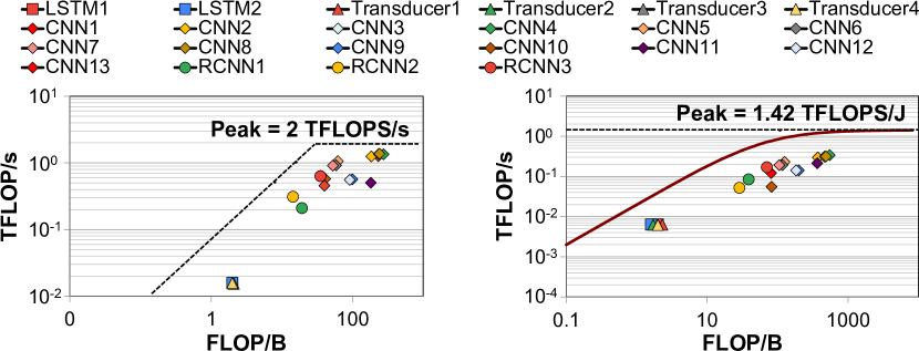
Figure 1: Throughput roofline (left) and energy roofline (right) for the Edge TPU across all Google edge neural network models.

2. Despite using specialized logic, the Edge TPU operates far below its theoretical maximum energy efficiency. We use a similar approach to prior work [12] to obtain a roofline for energy efficiency. Figure 1 (right) shows the roofline for the Edge TPU, along with the efficiency achieved for each model. We find that on average across all models, the Edge TPU achieves only 37.2% of its maximum possible energy efficiency. The energy efficiency is particularly low (33.8% of the maximum) for LSTM and Transducer models, but even the best CNN model achieves only 50.7% of the maximum efficiency.

3. The accelerator’s memory system design is neither effective nor efficient. Figure 2 shows the energy breakdown during inference execution across different models. We make three key observations from this figure. First, the on-chip buffers (the activation buffer and the parameter buffer) account for a significant portion of both static and dynamic energy across all models. For example, for CNN models, 48.1% of the total static energy and 36.5% of the total dynamic energy is spent on accessing and storing parameters in the on-chip buffers. This is due to the large size of both buffers in the Edge TPU. Second, averaged across all models, the Edge TPU spends 50.3% of its total energy on off-chip memory accesses (which includes the DRAM energy and the off-chip interconnect energy). Third, for LSTMs and Transducers, the Edge TPU spends approximately three quarters of its total energy on DRAM accesses. This is because while the buffers consume a significant amount of area (79.4% of the total area) in the Edge TPU, they are ineffective at reducing off-chip memory accesses. Despite the large buffers, only 11.9% of the parameters for these models can fit into the buffer. This is due to the parameter access patterns exhibited by LSTMs and Transducers: even if we ignore area constraints and increase the buffer capacity to 8x that of the Edge TPU, the buffer effectively caches only 46.5% of the parameters (an increase of only 3.9x). Due to ineffective caching, the 8x buffer decreases latency by only 37.6%, and energy consumption by only 40.3%. Overall, we conclude that the Edge TPU’s overall memory system (which includes both on-chip buffers and off-chip memory) is highly inefficient, and results in significant energy consumption.

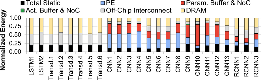
Figure 2: Energy breakdown during inference execution.

3.2 Layer-Level Study of Google Edge Models

To understand where the Edge TPU’s shortcomings (Section 3.1) come from, we analyze the models in significant detail, at the granularity of individual layers.

3.2.1 Analysis of LSTMs and Transducers

We identify three key properties of LSTMs and Transducers in our edge model analysis.

1. Large parameter footprint. Each gate in an LSTM cell has an average of 2.1 million parameters, which includes parameters for both input ($W_{x}$) and hidden ($W_{h}$) matrices (as shown in Figure 3, left). The large parameter footprint of LSTM gates results in large footprints for LSTM layers (up to 70 million parameters), and in turn, LSTM and Transducer models that include such layers. Figure 3 (right) shows the total footprint vs. the $\mathrm{FLOP}\text{/}\mathrm{B}$ ratio (which indicates arithmetic intensity) across the layers of representative CNNs, LSTMs, and Transducers (the trend is the same across all models). We observe from the figure that layers from LSTMs and Transducers have significantly larger footprints (with an average footprint of $33.4\text{\,}\mathrm{MB}\text{/}$) than layers from CNNs.

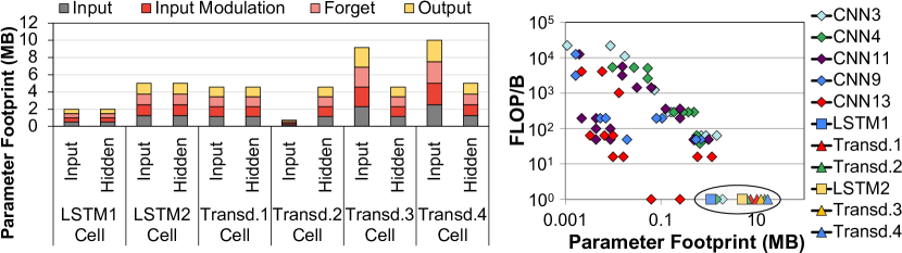
Figure 3: Parameter footprint of $W_{x}$ and $W_{h}$ for different LSTM gates for LSTMs and Transducers (left). Layer parameter footprint ($W_{x}$ and $W_{h}$ combined) vs. $\mathrm{FLOP}\text{/}\mathrm{B}$, with LSTM/Transducer layers circled (right).

2. No data reuse and low computational complexity. For these layers, the $\mathrm{FLOP}\text{/}\mathrm{B}$ for parameters (which includes both $W_{x}$ and $W_{h}$) is one (Figure 3, right). This is because the Edge TPU fetches $W_{x}$ and $W_{h}$ for each LSTM gate from DRAM, accesses them once to perform the input and hidden MVMs for that gate, and then does not touch the parameters again until the next LSTM cell computation, resulting in no reuse. In addition to the lack of reuse, LSTM and Transducer layers have much lower computational complexity than CNN and RCNN layers, with 67% fewer MAC operations on average.

3. Intra- and inter-cell dependencies. Two types of dependencies exist within LSTM layers, both of which affect how the accelerator schedules LSTM gates. First, inter-cell dependencies exist because a cell with state $c_{t}$ needs the hidden vector from the previous cell ($h_{t-1}$; see Section 2) to perform the required MVMs for the four LSTM gates that make up the cell. Second, intra-cell dependencies exist because the hidden vector of the current cell ($h_{t}$) is computed using the outputs of the four LSTM gates in the cell, and thus cannot start until the cell state ($c_{t}$) is updated. To respect these dependencies, the accelerator schedules cell computation in a sequential manner. Recall from Section 2 that each LSTM gate requires two MVMs: the input MVM and the hidden MVM. In order to compute these MVMs and respect dependencies, the Edge TPU treats each gate as two fully-connected (FC) layers (corresponding to input MVM and hidden MVM), and runs the gates sequentially.

However, we find that this scheduling is inefficient. Specifically, the Edge TPU misses opportunities for parallelizing computation across the gates of a single cell. Instead, by treating the gates as multiple FC layers, the Edge TPU employs the same default layer serialization used for FC layers. While this ensures correctness for actual FC layers, this hurts LSTM performance, as the PEs to spend more time waiting for the MVMs to be completed due to the unnecessary serialization, which degrades PE utilization. The lack of optimized support for LSTM cell computation results in significant missed opportunities to address LSTM performance and energy inefficiency.

3.2.2 Analysis of CNNs

Our analysis of edge CNN models reveals two new insights. First, unlike layers in traditional CNNs (e.g., AlexNet [57], VGG [86]), which tend to be relatively homogeneous, we find that the layers in edge CNN models exhibit significant heterogeneity in terms of type (e.g., depthwise, pointwise), shape, and size. This is often because these edge models employ several decomposition techniques [41, 44] to reduce the computational complexity and footprint of layers, in order to make them more friendly for the constrained edge devices. As an example of layer diversity, Figures 4 and 5 show the number of MAC operations and parameter footprint across different layers for four CNN models. We find that the MAC intensity and parameter footprint vary by a factor of 200x and 20x across different layers, indicating how significant the diversity is for important layer characteristics.

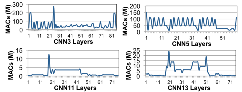
Figure 4: MAC operation count in different layers of four CNN models.

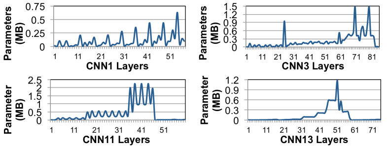
Figure 5: Parameter footprint in different layers of four CNN models.

Second, we find that layers exhibit significant variation in terms of data reuse patterns for parameters and for input/output activations. For example, a layer in a CNN can sometimes break down an input into multiple filtered channels (e.g., breaking an image down into red, green, and blue colors. A pointwise layer operates on $K$ different channels, and performs convolution using the same input activations on each of these channels. In comparison, a depthwise layer operates on only a single channel, and is unable to reuse its input activations. We also observe variation in data reuse across layers of the same type. For example, initial/early standard convolution layers in edge CNNs have a shallow input/output channel depth, large input activation width/height, and very small kernels, resulting in very high parameter reuse. In comparison, standard convolution layers that are placed toward the end of the network have a deep input and output channel depth, small input activation width/height, and a large number of kernels, resulting in very low parameter reuse. This variation in reuse is illustrated in Figure 3 (right), which shows that the $\mathrm{FLOP}\text{/}\mathrm{B}$ ratio varies across different layers for five representative CNN models by a factor of 244x.

3.2.3 Analysis of RCNNs

RCNNs include layers from both CNNs and LSTMs. As a result, individual layers from RCNN models exhibit the same characteristics we describe above for LSTM and CNN layers. We find that layers from RCNNs exhibit significantly higher footprints and lower $\mathrm{FLOP}\text{/}\mathrm{B}$ ratios than CNN layers, as an RCNN model includes both LSTM and CNN layers. Due to the inclusion of both layer types, we observe significantly more variation across RCNN layers characteristics as well.

3.2.4 Sources of Edge TPU Shortcomings

Using insights from our comprehensive model analysis in Section 3.2, we can now provide more insight into the sources of the Edge TPU shortcomings identified in Section 3.1.

PE Underutilization. We identify three reasons why the actual throughput of the Edge TPU falls significantly short of the peak. First, while some layers have high parameter reuse (e.g., pointwise layers, with a $1200\text{\,}\mathrm{FLOP}\text{/}\mathrm{B}$ ratio), other layers exhibit very low reuse ($164\text{\,}\mathrm{FLOP}\text{/}\mathrm{B}$) while at the same time having large parameter footprints ($0.55\text{\,}\mathrm{MB}\text{/}$). Layers with low reuse yet large footprints for parameters often leave PEs idle, as the parameters incur long-latency cache misses to DRAM. The bandwidth of modern commercial DRAM (e.g., $32\text{\,}\mathrm{GB}\text{/}\mathrm{s}$ for LPDDR4 [48]) is two orders of magnitude below the $2\text{\,}\mathrm{TB}\text{/}\mathrm{s}$ bandwidth needed to sustain peak PE throughput when only one $\mathrm{FLOP}\text{/}\mathrm{B}$ is performed (as is the case for LSTM layers; see Section 3.2.1). Many layers end up with a similar memory bandwidth bottleneck during execution.

Second, the Edge TPU does not provide a custom dataflow optimized for each layer. As we identified in Section 3.2, layers both across and within models exhibit high variation in terms of data reuse patterns. This variation necessitates the need for different dataflows for different layers, where each dataflow exposes a different set of reuse opportunities for parameters and activations. However, state-of-the-art accelerators such as the Edge TPU employ a single dataflow that is designed for high spatial/temporal reuse [58, 26, 20, 73, 9]. The missed reuse opportunities in many of the model layers causes PEs to needlessly wait on retrieving previously-accessed data that was not properly retained on-chip.

Third, the different shapes and inter-/intra-layer dependencies across different types of layers (e.g., LSTM cell, standard convolution, depthwise, pointwise, fully-connected) makes it challenging to fully utilize a PE array with a fixed size, which is the case in state-of-the-art accelerators (e.g., [9, 26, 73, 20]). To cater to these differences across layers, there is a need for both better scheduling of MVM computation (e.g., uncovering parallel computation opportunities as we found in Section 3.2.1) and appropriately sizing the PE arrays based on the needs of specific layers in order to maintain efficient utilization.

Poor Energy Efficiency. We find three major sources of energy efficiency in the Edge TPU. First, the Edge TPU incurs high static energy costs because (1) it employs a large overprovisioned on-chip buffer, and (2) it underutilizes PEs. Second, the on-chip buffers consume a high amount of dynamic energy, as we saw for CNN layers in Section 3.1. Third, the Edge TPU suffers from the high cost of off-chip parameter traffic. On-chip buffers fail to effectively cache parameters for many layers due to layer diversity, causing 50.3% of the total inference energy to be spent on off-chip parameter traffic (see Section 3.1).

Memory System Issues. We uncover two large sources of memory system inefficiency. First, due to layer diversity, on-chip buffers are ineffective for a large fraction of layers. As we discuss in Section 3.2.1, LSTM gates have large parameter footprints and zero parameter reuse, rendering the on-chip buffer useless for a majority of LSTMs and Transducers, and for a significant fraction of RCNN layers (i.e., models that incorporate LSTM layers). For CNN layers, we find that those layers with low data reuse account for a significant portion of the entire model parameters (e.g., 64% for CNN6). This means that the on-chip buffer fails to cache a large portion of the parameters for CNN models. As a result, despite being $4\text{\,}\mathrm{MB}\text{/}$ in size, the on-chip parameter buffer is effective only for a small fraction of layers, which have an average parameter footprint of only $0.21\text{\,}\mathrm{MB}\text{/}$.

Second, even layers with high data reuse incur significant costs when they access on-chip buffers. This is because the on-chip parameter buffer is very large, even though the layers that benefit from caching in the buffer have small parameter footprints. These layers exhibit high parameter reuse, and thus generate a large number of buffer accesses. Unfortunately, because of the large size of the buffer, every access incurs a high dynamic energy cost. As a result, this unneeded capacity for the high-data-reuse layers results in wasted energy for buffer accesses.

3.3 Key Takeaways

Our analysis provides three key insights: (1) there is significant variation in terms of layer characteristics across and within state-of-the-art Google edge models; (2) the monolithic design of the Edge TPU is the root cause of its shortcomings and the resulting large inefficiency; and (3) to achieve high utilization and energy efficiency, all key components of an edge accelerator (PE array, dataflow, on-chip memory, off-chip memory bandwidth) must be customized to different layer characteristics.

4 Mensa Framework

Mensa is a new machine learning accelerator design framework that harnesses inter- and intra-layer variation across edge NN models for high efficiency and high performance.

4.1 High-Level Overview

The key idea of Mensa is to distribute the layers from an NN model across a collection of smaller hardware accelerators that are carefully specialized towards the properties of different layer types. By specializing each accelerator to a subset of layers, Mensa avoids the shortcomings of current monolithic edge ML accelerators, resulting in a highly-efficient and high-performance accelerator with a much smaller area. Mensa consists of (1) a collection of heterogeneous hardware accelerators; and (2) a runtime scheduler that determines which accelerator each layer in an NN model should execute on, using a combination of NN model and hardware characteristics. As we show in Section 5, Mensa designs typically need to employ only a small number of accelerators, as layers tend to group together into a small number of layer families.

We design Mensa as a framework that can support a wide range of architectural implementations. This allows Mensa to (1) be optimized to specific system needs, which is critical to keep resource utilization to a minimum in resource-constrained edge devices; and (2) adapt easily to future types of NN models that we expect will arise in the future. We discuss one example implementation of Mensa in Section 5, which caters to the Google edge NN models that we analyze (Section 3), to illustrate the effectiveness of our framework.

4.2 Mensa Runtime Scheduler

The goal of Mensa’s software runtime scheduler is to identify which accelerator each layer in an NN model should run on. Each of the accelerators in Mensa caters to one or more families of layers, where these families share specific characteristics (e.g., layer type, footprint, data reuse, dependencies). For a given Mensa implementation, the scheduler has two pieces of information (which can be maintained in a hardware driver): (1) the characteristics of each layer family; and (2) which hardware accelerator is best suited for each family.

Layer-to-Accelerator Mapping. When an NN model runs on Mensa, the scheduler generates a mapping between each NN layer and different accelerators. The scheduler uses the NN model (including a directed acyclic graph that represents communication across model layers) and the configuration information in the driver to determine this mapping. The mapping is generated in two phases.

In Phase I, the scheduler iterates through each layer in the model, and identifies the ideal hardware accelerator for each layer in isolation (i.e., without considering communication overhead). The scheduler determines two properties for each layer: (1) the cluster that the layer belongs to, and (2) the target accelerator for the layer. While the goal of Phase I is to maximize accelerator throughput and energy efficiency for each layer, the resulting schedule may be sub-optimal for efficiency, because it does not consider the overhead of transferring activations or communicating dependencies (e.g., $h_{t}$ in LSTM cells) between different layers. This can have a large impact on the overall system performance and energy if the amount of communication is large.

In Phase II, our scheduler accounts for the communication overhead using a simple cost analysis algorithm, and assigns the destination accelerator for each layer. Phase II iterates through each of the layers in a model sequentially, and we describe the decisions made during Phase II for an arbitrary layer $i$, which are performed after layer $i-1$’s destination accelerator (destination $i-1$) has been assigned. For layer $i$, Phase II determines whether the layer should be scheduled on (1) its ideal accelerator, as determined by Phase I; or (2) destination $i-1$. Destination $i-1$ is used whenever the costs of communicating operands to the ideal accelerator outweigh the penalties of executing layer $i$ on destination $i-1$, which is a sub-optimal accelerator for the layer. There are two cases where Phase II assigns layer $i$ to its ideal accelerator. First, if the number of MAC operations required for layer $i$ is 2x higher (determined empirically) than the compute resources available in destination $i-1$, running the layer on destination $i-1$ would incur increased performance and energy costs over using the ideal accelerator. Second, if the amount of parameter data that destination $i-1$ would need to fetch to run layer $i$ is greater than the amount of output activation data that would have to be sent to the ideal accelerator, and the opportunities for reusing the parameter data in destination $i-1$ are low ($\mathrm{FLOP}\text{/}\mathrm{B}$ $<64$, determined empirically), running the layer on destination $i-1$ would incur off-chip memory overheads (with few opportunities for amortizing these overheads) compared to using the ideal accelerator. In all other cases, Phase II assigns layer $i$ to destination $i-1$.

Mensa uses a heuristic-based approach that may not always achieve the best mapping decisions that a hypothetical oracle scheduler could produce. However, our heuristic-based scheduler still achieves significant performance and energy improvements (Section 7), while being practical to implement in edge devices. We leave the exploration of better scheduling algorithms to future work.

Execution and Communication. Once Phase II of the scheduler is complete, Mensa begins model execution using the generated layer-to-accelerator mapping. During execution, destination $i$ needs to read (1) any unbuffered parameters (i.e., weights) from DRAM; and (2) input activations (i.e., input data) produced by layer $i-1$, when layer $i$ is run on a different accelerator than layer $i-1$. In order to simplify communication between accelerators, Mensa accelerators transfer activations to another accelerator through DRAM, avoiding the need to keep on-chip data coherent across accelerators (or, when some of the Mensa accelerators are placed near memory, to keep on-chip and near-data accelerators coherent [5, 3]).

5 Mensa-G: Mensa for Google Edge Models

We now discuss Mensa-G, an example Mensa design optimized for our Google edge NN models. We start by identifying layer families in these models (Section 5.1). Using the unique characteristics for each family, we determine which characteristics have the greatest impact on accelerator design, and use that to guide the number of accelerators that we need for Google edge NN models (Section 5.2).

5.1 Identifying Layer Families

We revisit the NN edge models that we analyze in Section 3. For each layer, we study the correlation between different characteristics. These characteristics include (1) parameter reuse ($\mathrm{FLOP}\text{/}\mathrm{B}$), (2) parameter footprint ($\mathrm{MB}\text{/}$), and (3) MAC intensity (i.e., defined by the number of MAC operations). Figure 6 shows how parameter reuse ($\mathrm{FLOP}\text{/}\mathrm{B}$) correlates with the parameter footprint (Figure 6, left) and the number of MAC operations (Figure 6, right) for a representative set of layers from five CNNs, two LSTMs, and two Transducers. Based on all of the layer characteristics that we analyze, we observe across all layers from all models (not just the representative layers or correlations plotted) that 97% of the layers group into one of five layer families.

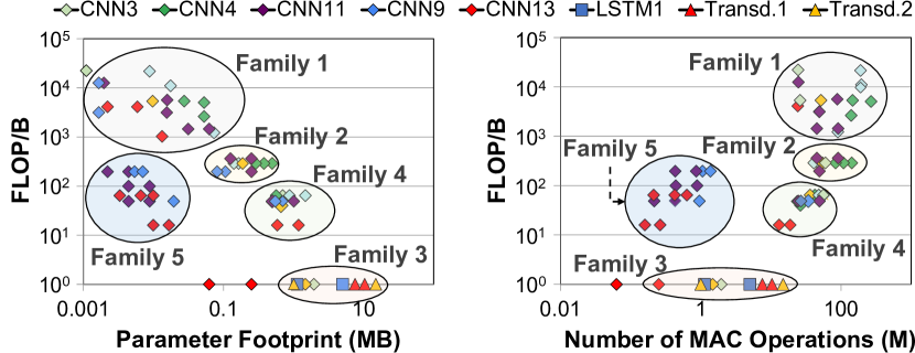
Figure 6: Parameter footprint vs. parameter reuse (left) and number of MAC operations vs. parameter reuse (right) across example layers.

Family 1. Layers in this family have (a) a very small parameter footprint ($1100\text{\,}\mathrm{kB}\text{/}$), (b) a very high $\mathrm{FLOP}\text{/}\mathrm{B}$ ratio for parameters (780–20K), and (c) high MAC intensity (30M–200M). These layers exhibit high activation footprints and high activation data reuse as well. A majority of layers in this family are standard convolutional layers with shallow input/output channels and large input activation width/height. We find that these layers are mostly found among early layers in CNNs and RCNNs, and typically achieve high PE utilization (on average 82%) on the Google Edge TPU because of their high MAC intensity and low memory use.

Family 2. Layers in this family have (a) a small parameter footprint ($100500\text{\,}\mathrm{kB}\text{/}$; 12x higher on average than Family 1), (b) a moderate $\mathrm{FLOP}\text{/}\mathrm{B}$ ratio for parameters (81–400; up to 10x lower than Family 1), and (c) high MAC intensity (20M–100M). These layers exhibit high activation footprints and activation data reuse as well. Many of the layers belong to pointwise layers, which have high parameter reuse due to convolving 1x$K$ filters (where $K$ is the input channel depth, i.e., the number of channels) with input activations across different channels. Other layers in the family include standard convolution layers commonly found in the middle of CNN networks, with deeper input/output channels and smaller activation width/height than the convolution layers in Family 1, We find that Family 2 layers have lower PE utilization (64%) than layers in Family 1 on the Google Edge TPU, because the lower parameter reuse reduces opportunities to amortize the off-chip memory access overheads.

Family 3. Layers in this family have (a) a very large parameter footprint ($0.918\text{\,}\mathrm{MB}\text{/}$), (b) minimal $\mathrm{FLOP}\text{/}\mathrm{B}$ ratio for parameters, and (c) low MAC intensity (0.1M–10M). These layers also exhibit small activation footprints but high activation reuse. The majority of these layers are from LSTM gates in LSTMs and Transducers, or are fully-connected layers from CNNs. These layers have very low PE utilization (0.3% on average) on the Google Edge TPU, as there are not enough MAC operations to hide the significant off-chip memory bottlenecks incurred while retrieving parameters.

Family 4. Layers in this family have (a) a relatively large parameter footprint ($0.52.5\text{\,}\mathrm{MB}\text{/}$), (b) low-to-moderate $\mathrm{FLOP}\text{/}\mathrm{B}$ ratio for parameters (25–64), and (c) moderate MAC intensity (5M–25M). These layers exhibit small activation footprints but high activation reuse. A large portion of layers in this category are standard convolutional layers with deep input/output channels and input activation width/height, along with a large number of kernels. Family 4 layers have a low PE utilization (32% on average) on the Google Edge TPU, as the large parameter footprint and relatively low parameter reuse generate significant off-chip memory traffic, and the moderate MAC intensity hides only some of the memory access bottlenecks.

Family 5. Layers in this family have (a) a very small parameter footprint ($1100\text{\,}\mathrm{kB}\text{/}$), (b) a moderate $\mathrm{FLOP}\text{/}\mathrm{B}$ ratio for parameters (49–600), and (c) low MAC intensity (0.5M–5M). These layers exhibit high activation footprints but have almost zero activation data reuse. Many of the layers in Family 5 are depthwise convolution layers. Such layers have only one channel, and thus do not reuse activations, and typically have only a small number of filters (where each filter consists of one or more kernels) that are applied to all slices of the inputs, resulting in high parameter reuse. Family 5 layers achieve a low average PE utilization of 21% on the Google Edge TPU, as the increased parameter reuse compared to Family 4 is offset by the reduced MAC intensity, and Family 5 layers still have limited opportunities to hide the memory access bottlenecks.

5.2 Hardware Design Principles and Decisions

As we study the distinguishing characteristics of each of the five layer families, we find that some characteristics have a strong influence on the hardware design, while others do not necessitate significant changes to the hardware. We discuss two insights that drive our hardware design decisions.

First, we find that significantly different values of MAC intensity and parameter footprint/reuse lead to greatly different hardware to maximize efficiency, as they impact a number of key accelerator design parameters (e.g., PE array size, on-chip buffer size, memory bandwidth considerations). Looking at the five layer families, we identify that (a) layers in Families 1 and 2 share a high MAC intensity, small parameter footprint, and moderate-to-high parameter reuse; while (b) layers in Families 3 and 4 share a low MAC intensity, large parameter footprint, and low parameter reuse. This means that we need at least two different accelerator designs: one that caters to the compute-centric behavior of Families 1/2 (see Section 5.3), and one that caters to the data-centric behavior of Families 3/4 (see Section 8). Given our resource-constrained edge environment, we look to see if layers in Family 5, which have a low MAC intensity (similar to Families 3 and 4) but a relatively small parameter footprint (similar to Families 1 and 2), can benefit from one of these two approaches. We find that the low MAC intensity, along with the low parameter reuse by many Family 5 layers, allow the layers to benefit from many of the non-compute-centric optimizations that benefit Families 3 and 4, so we study them collectively as we design the data-centric accelerators.

Second, a key distinguishing factor between different accelerator designs is the accelerator dataflow, as it dictates which reuse opportunities in layers are exploited, and thus strongly impacts PE utilization and energy efficiency. One prior work [58] analyzes the large dataflow design space, and discusses four types of data reuse: spatial multicasting (reading a parameter once, and spatially distributing it as an input to multiple PEs at the same time), temporal multicasting (replicating a parameter in a small local buffer, and delivering the parameter as multiple inputs at different times to the same PE), spatial reduction (accumulating activations from multiple PEs at the same time using multiple compute units), and temporal reduction (accumulating multiple activations generated at different times using a single accumulator/buffer). The chosen dataflow directly affects how the memory system and on-chip network of an accelerator should be designed. Thus, we need different dataflows for layer families with significantly different parameter and activation reuse patterns.

5.2.1 Determining the Number of Accelerators Needed

Both of our compute-centric layer families (Families 1 and 2) benefit from a similar dataflow, which exposes reuse opportunities for both parameters and activations. Between the compute-centric optimizations and the shared dataflow affinity, we determine that we can use a single accelerator (Pascal; Section 5.3) to efficiently execute layers from both Family 1 and Family 2.

Across our three data-centric layer families (Families 3, 4, and 5), we find that layers from both Families 4 and 5 benefit from a dataflow that exposes reuse opportunities for parameters but not for activations, and can use a single accelerator (Jacquard; Section 5.5). Family 3 layers exhibit different data reuse characteristics, and they benefit from a dataflow that provides temporal reduction opportunities for activations. As a result, they benefit from a separate accelerator (Pavlov; Section 5.4).

5.2.2 Template-Based Design Approach

We employ a template-based design approach for the compute- and data-centric accelerators: while we design each accelerator so that it is based on layer families’ characteristics, we use the same generic tiled architecture for each accelerator as the baseline edge TPU. We do this to ease the integration of our hardware into a real system: from the perspective of compilers and programs, each of our accelerators appears to be just a different instance (with a different configuration) of a single baseline accelerator (the Edge TPU). This is a critical design decision: it allows us to deploy and run models using existing highly-optimized design/compile toolchains (e.g., the Google Edge TPU compiler [27]) seamlessly on all of Mensa’s accelerators, but it also limits the degree of customization (and, thus, efficiency) each of our accelerator designs can achieve. While the Mensa framework easily allows the design of accelerators that do not employ this tiled architecture, we make this design choice to reduce the burden on the software stack (e.g., more complex compilers, multiple libraries for programmers).

The three accelerators in Mensa-G are designed to be independent: we customize each accelerator’s dataflow, on-chip memory (i.e., buffers), and access to off-chip memory for the layers that the accelerator targets, and carefully provision the number of PEs and design the interconnect to support the chosen dataflow and memory access patterns. To simplify the design and increase modularity, we do not share any resources between accelerators.

5.3 Pascal: Compute-Centric Accelerator Design

Pascal caters to layers in Families 1 and 2, which are compute-centric. We establish two requirements for the design of Pascal. First, the design should exploit opportunities available across layers in Families 1 and 2 for the temporal reduction of output activations. The temporal reduction mitigates the impact of the large output activation footprint, by reducing the off-chip memory bandwidth requirements and providing an opportunity to reduce the buffer capacity needed for activations. Second, the design should avoid spatial reduction for output activations. Spatial reduction generates partial output sums in each PE, and then gathers all of the partial sums by sending them across the on-chip network to a single PE. Given the large footprint of output activations, this partial sum traffic often saturates the limited bandwidth of the on-chip network, which can leave the PEs underutilized and lead to significant performance and energy penalties. Based on these two requirements, we design Pascal as shown in Figure 7a.

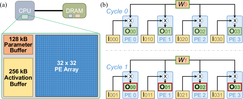
Figure 7: (a) Pascal design; (b) Pascal dataflow for a pointwise layer.

Dataflow. Figure 7b shows the dataflow that we design for Pascal. In the figure, we show how the dataflow works for an example pointwise layer in a CNN, where the layer has $K$ channels. For each channel, every element in the matrix is multiplied by a single parameter (i.e., a weight representing a filter is applied point by point). In the output activation matrix $O$, each element $O_{ij}$ (where $i$ is the row, and $j$ is the column) is computed as the sum of $I_{ijk}\times W_{k}$ over every channel $k$, where $I$ is a three-dimensional matrix of input activations and $W$ is a vector of weights.

As shown in Figure 7b, Pascal’s dataflow reduces memory traffic by enabling two types of reuse. First, the dataflow uses temporal reduction for each output activation element $O_{ij}$ without using spatial reduction, by instead having a single PE accumulate the entire sum of the element across multiple cycles in the PE’s private register file. We indicate temporal reuse (i.e., temporal multicasting) in the dataflow using a red border and bold text in the figure. Second, the dataflow uses spatial multicasting for each parameter $W_{k}$, by ensuring that all of the PEs are working on the same channel $k$ in the same cycle. We indicate spatial multicasting using a green border and italic text in the figure.

PE Array. We size the PE array in Pascal based on two attributes. First, there should be enough PEs to accommodate the high MAC intensity exhibited by layers in Families 1 and 2. Second, all PEs should ideally operate on the same parameter in a single cycle, to minimize parameter bandwidth. To account for both attributes, and to ensure a good balance between PE utilization, inference latency, and energy consumption, we profile the performance of Family 1/2 layers on different PE sizes, and empirically choose a 32x32 PE array, which lets Pascal achieve a $2\text{\,}\mathrm{TFLOP}\text{/}\mathrm{s}$ peak throughput.

Memory System. Figure 7a shows the on-chip buffers used in Pascal. These buffers are significantly smaller than those in the Google Edge TPU. We reduce the size of the activation buffer from $2\text{\,}\mathrm{MB}\text{/}$ in the Edge TPU to $256\text{\,}\mathrm{kB}\text{/}$ in Pascal, because Pascal’s dataflow exploits temporal reduction for the output activations using the internal PE registers, and no longer needs to store the large footprint of the output activations in the activation buffer. We reduce the size of the parameter buffer from $4\text{\,}\mathrm{MB}\text{/}$ in the Edge TPU to $128\text{\,}\mathrm{kB}\text{/}$ in Pascal, because layers in Families 1 and 2 have small parameter footprints. Given the low off-chip memory bandwidth requirements of Pascal, we keep the accelerator on the CPU die.

5.4 Pavlov: LSTM-Centric Accelerator Design

Pavlov caters to layers in Family 3, which are data-centric and predominantly consist of LSTM layers. We establish two requirements for the design of Pavlov. First, the design should exploit output activation reuse opportunities in Family 3 layers. Second, the design should reduce the off-chip memory bandwidth required by parameters. These layers have a very large parameter footprint, and parameters that are cached in the parameter buffer of the Google Edge TPU are evicted before they can be reused, forcing every parameter access to go to main memory. Based on these two requirements, we design Pavlov as shown in Figure 8.

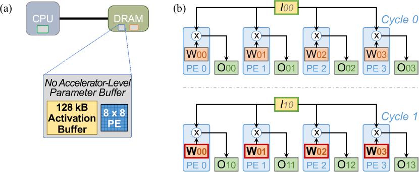
Figure 8: (a) Pavlov design; (b) Pavlov dataflow.

Dataflow. Figure 8b shows the dataflow that we design for Pavlov. Recall from Section 2 that an LSTM layer has multiple cells, each containing four gates. Each gate performs two MVMs (an input MVM, which multiplies the input parameter matrix $W_{x}$ with the input vector $x_{t}$; and a hidden MVM, which multiplies the hidden parameter matrix $W_{x}$ with the hidden input vector $h_{t-1}$, across a sequence of samples over time ($t$). To generalize the figure for both MVMs, we show a single MVM between a parameter matrix $W$ (where each element $W_{ij}$ is located at row $i$, column $j$) and an input activation vector set $I$ (where each element $I_{ti}$ is the located at row $i$ in the input activation vector for time $t$), where $I\times W=O$ ($O$ is the output vector set for a particular gate).

As shown in Figure 8, Pavlov’s dataflow reduces memory traffic by enabling two types of reuse. First, the dataflow temporally reuses a weight $W_{ij}$. We observe that in an LSTM layer, instead of iterating one cell at a time (where we compute the input MVMs and hidden MVMs for the four gates), we can compute the input MVMs for all $C$ cells in the layer back-to-back, and then compute the hidden MVMs for all four gates. This allows the dataflow to fetch each element of $W$ only once per layer (as opposed to fetching each element $4TC$ times, once for every sample $t$ for each of the four gates, over $C$ cells). To enable the temporal reuse of the weight, the PE stores the weight in one of its private registers, and stores $C$ partial sums (which are accumulated over time to generate $C$ outputs for each cell in the layer). We indicate temporal reuse (i.e, temporal multicasting) in the dataflow using a red border and bold text in the figure. Second, the dataflow uses spatial multicasting for each input activation $I_{ti}$, as the same activation is multiplied across all columns of $W$ for a given row $i$. We indicate spatial multicasting using a green border and italic text in the figure.

PE Array. Because Family 3 layers have low MAC intensity, and mainly perform MVM, we design a much smaller PE array for Pavlov than that in the Google Edge TPU. We analyze the inference latency across a range of PE array sizes, and empirically choose an 8x8 array size to balance latency, utilization, and energy. This allows Pavlov to achieve a $128\text{\,}\mathrm{GFLOP}\text{/}\mathrm{s}$ peak throughput.

Memory System. We decide to place Pavlov inside memory [71, 24, 23], to accommodate the significant off-chip memory bandwidth requirements of Family 3 layers. Modern 3D-stacked memories such as High-Bandwidth Memory [47] and the Hybrid Memory Cube [43] include logic layers that have access to the high memory bandwidth available within a 3D-stacked memory chip. By placing Pavlov in the logic layer of a 3D-stacked memory chip, we can provide Family 3 layers with much higher bandwidth than the external memory bandwidth.

Given that parameters and activations from Family 3 layers exhibit different characteristics, we customize separate on-chip buffers for each data type, as shown in Figure 8a. For parameters, we use only one level of memory hierarchy ($512\text{\,}\mathrm{B}\text{/}$ of private registers per PE), eliminate the parameter buffer, and stream parameters directly from DRAM. The per-PE registers provide enough space to cache the temporally-multicasted parameters, and there are no other reuse opportunities that an accelerator-level parameter buffer could exploit (because the parameters have a very large footprint). For activations, thanks to the small activation footprint of layers in Family 3, we use a $128\text{\,}\mathrm{kB}\text{/}$ buffer.

5.5 Jacquard Accelerator Design

Jacquard caters to layers in Families 4 and 5, which primarily consist of non-LSTM data-centric layers. We establish two requirements for the design of Jacquard. First, the design should exploit temporal reuse opportunities for parameters in layers from Families 4 and 5. Second, the design should provide high off-chip memory bandwidth, as the parameter footprint is high for many (but not all) of the layers. Based on these two requirements, we design Jacquard as shown in Figure 9.

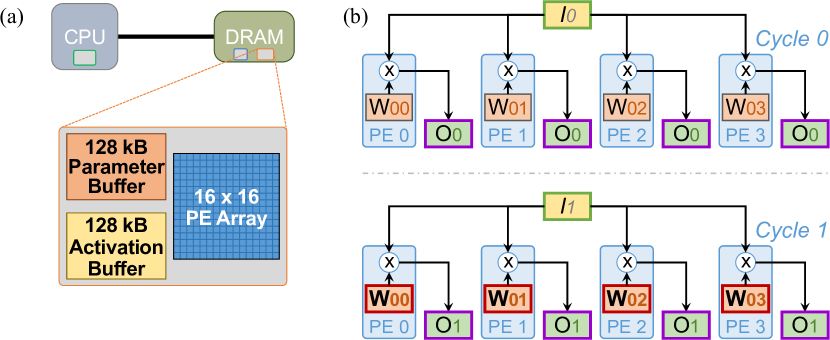
Figure 9: (a) Jacquard design; (b) Jacquard dataflow.

Dataflow. Figure 8c shows the dataflow that we design for Pavlov. We illustrate the dataflow using a generic MVM, where an input activation vector $I$ is multiplied by a parameter matrix $W$ to generate an output activation vector $O$. As shown in the figure, Jacquard’s dataflow reduces memory traffic by enabling two types of reuse. First, the dataflow temporally reuses a parameter $W_{ij}$. Jacquard uses the same temporal reuse approach as Pavlov, where a parameter is stored in a PE register and reused (i.e., temporally multicast) over multiple cycles to reduce the number of times the parameter is fetched from memory. By increasing the reuse of the parameter, the dataflow effectively hides the off-chip memory access latency by overlapping it completely with PE computation. We indicate temporal reuse in the dataflow using a red border and bold text in the figure. Second, the dataflow uses spatial multiicasting for each input activation $I_{i}$. We indicate spatial multicasting using a green border and italic text. In order to enable spatial multicasting for layers in Families 4 and 5, the dataflow has all PEs collectively compute a single output activation, by having each PE compute a partial sum (indicated in the figure with a purple border), and then using the on-chip interconnect to gather the partial sums and produce the final output activation.

PE Array. While layers in Families 4 and 5 have low MAC intensity, they perform more MAC operations on average than Family 3 layers. Our analysis of PE array sizes shows that equipping Jacquard with an array smaller than 16x16 increases the latency, so we empirically select 16x16 for the array size. This allows Jacquard to achieve a peak throughput of $512\text{\,}\mathrm{GFLOP}\text{/}\mathrm{s}$.

Memory System. Similar to Pavlov, we decide to place Jacquard inside the logic layer of 3D-stacked memory. Doing so enables high memory bandwidth for the large parameter footprints of Family 4 layers. We use separate shared buffers for each data type, as shown in Figure 9a. Given the small activation footprints, we use a small $128\text{\,}\mathrm{kB}\text{/}$ buffer for them (a 16x reduction compared to the Google Edge TPU). Thanks to the temporal parameter reuse that Jacquard’s dataflow enables, we can reduce the parameter buffer size to $128\text{\,}\mathrm{kB}\text{/}$ (a 32x reduction compared to the Google Edge TPU).

5.6 Data Transformations & Communication

The three accelerators in Mensa-G are designed to replace the core of the Edge TPU (i.e., the monolithic PE array and interconnect). Our Mensa implementation maintains all of the other hardware support from the overall Edge TPU architecture. Notably, Mensa supports the same data transform operations (e.g., the im2col operation for convolution, which takes the current window of pixels being processed in an image and converts the data layout into a matrix column) that the Edge TPU currently performs. Such data transform operations are typically handled during local data exchanges between the PEs.

In Mensa-G, the accelerators communicate with each other only in-between layer execution, as layers do not execute concurrently (see Footnote 4), and each layer executes completely in a single accelerator. We observe that Google edge models typically communicate between accelerators only 4–5 times during execution. Three of our models (CNN5, CNN6, CNN7) communicate significantly more frequently than average, as they include a large number of skip connections (i.e., layer $i$ takes in data that was output by layer $i-j$, where $j>1$). Mensa schedules the layers from these models across multiple accelerators, and the target accelerator has to fetch information produced by early layers (e.g., output feature maps) from either off-chip memory or from another accelerator’s on-chip buffer (if the data has not yet been evicted). Mensa’s scheduler coordinates this inter-layer and inter-accelerator communication, and our evaluations take the extra communication traffic into account.

6 Experimental Methodology

Models. The 24 Google edge NN models that we analyze are used in several Google mobile applications/products, such as image classification, object detection, semantic segmentation, automatic speech recognition, and image captioning. The models are specifically developed for edge devices using TensorFlow Lite [28], and are fully 8-bit quantized using quantization-aware training [29]. The models are then compiled using the Google Edge TPU compiler [27]. We expect to see similar results for popular publicly-available models such as MobileNet [41] and ResNet [38], which share similarities with some of our edge models.

Energy Analysis. We build our energy model based on prior works [4, 20, 5], which sums up the total energy (including both static and dynamic energy) consumed by the accelerator, DRAM, off-chip and on-chip interconnects, and all on-chip buffers. We use CACTI-P 6.5 [70] with a $22\text{\,}\mathrm{nm}\text{/}$ process technology to estimate on-chip buffer energy. We assume that each 8-bit MAC unit consumes $0.2\text{\,}\mathrm{pJ}\text{/}\mathrm{bit}$. We model the DRAM energy as the energy consumed per bit for LPDDR4 [48], based on models from prior works [20, 4].

Performance Analysis & Simulation. We use an in-house simulator to faithfully model all major components of the Google Edge TPU, including the PE array, memory system, on-chip network, and dataflow. We heavily modify the simulator to implement our three proposed accelerators and the software runtime of Mensa. We develop an analytical cost model to determine the performance of each of our proposed dataflows, and integrate the dataflow performance numbers into our simulator’s performance model. We use CACTI-P 6.5 [70] to determine the on-chip buffer latencies for each proposed accelerator. Similar to prior works [4, 20, 16, 5], the accelerators in the logic layer of 3D-stacked memory have access to the $256\text{\,}\mathrm{GB}\text{/}\mathrm{s}$ internal bandwidth of High-Bandwidth Memory (HBM) [47], which is 8x the external memory bandwidth to accelerators that sit outside of memory. In our evaluation, we assume that both the Edge TPU baseline and Mensa have access to $2\text{\,}\mathrm{GB}\text{/}$ of HBM DRAM.

7 Evaluation

We evaluate inference energy (Section 7.1), hardware utilization and throughput (Section 7.2), and inference latency (Section 7.3) of four configurations: (1) Baseline, the Google Edge TPU; (2) Base+HB, a hypothetical version of Baseline with 8x the memory bandwidth ($256\text{\,}\mathrm{GB}\text{/}\mathrm{s}$); (3) Eyeriss v2, a state-of-the-art edge accelerator [9] that uses reconfigurable interconnects to partially address CNN model heterogeneity; and (4) Mensa-G (from Section 5) with all three proposed accelerators (Pascal, Pavlov, Jacquard). To improve figure clarity, we show individual model results for only a few representative models of each model type. Our average results are reported across all 24 Google edge NN models.

7.1 Energy Analysis

Figure 10 (left) shows the total inference energy consumed by the four systems we evaluate across different NN models. We make three observations from the figure.

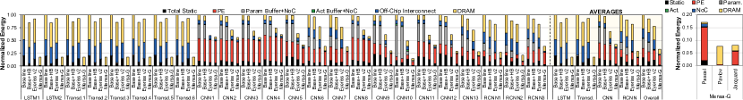
Figure 10: Inference energy across different models (left) and energy breakdown across our three proposed accelerators (right), normalized to Baseline.

First, providing high memory bandwidth to Baseline (Base+HB) results in only a small reduction in energy (7.5% on average). This is because Base+HB still incurs a high energy cost due to (1) on-chip buffers that are overprovisioned for many layers, and (2) off-chip traffic to DRAM. Base+HB benefits LSTMs and Transducers the most (14.2% energy reduction), as the higher memory bandwidth significantly reduces the inference latency of these models, which in turn lowers static energy.

Second, Eyeriss v2 suffers from significant energy inefficiency for LSTMs and Transducers. While Eyeriss v2 lowers static energy compared to Baseline, due to its use of a much smaller PE array (384 vs. 4096) and on-chip buffers ($192\text{\,}\mathrm{kB}\text{/}$ vs. $4\text{\,}\mathrm{MB}\text{/}$), it still incurs the high energy costs of large off-chip parameter traffic to DRAM. Averaged across all LSTM and Transducer models, Eyeriss v2 reduces energy by only 6.4% over Baseline. For CNN models, Eyeriss v2 reduces energy by 36.2% over Baseline, as its smaller on-chip buffer significantly reduces dynamic energy consumption.

Third, Mensa-G significantly reduces energy across all models. The reduction primarily comes from three sources. (1) Mensa-G lowers the energy spent on on-chip and off-chip parameter traffic by 15.3x over Baseline, by scheduling each layer on the accelerator with the most appropriate dataflow for that layer. LSTMs and Transducers benefit the most, as their energy in both Base+HB and Eyeriss v2 is dominated by off-chip parameter traffic, which Pavlov and Jacquard drastically reduce by being placed inside memory. (2) Mensa-G reduces the dynamic energy of the on-chip buffer and network (NoC) by 49.8x and 6.2x over Base+HB and Eyeriss v2, by avoiding overprovisioning and catering to specialized dataflows. This is most beneficial for CNN and RCNN models. (3) Mensa-G reduces static energy by 3.6x and 5.6x over Base+HB and Eyeriss v2, thanks to using significantly smaller PE arrays that avoid underutilization, significantly smaller on-chip buffers, and dataflows that reduce inference latency.

Eyeriss v2 falls significantly short of Mensa’s energy efficiency for three reasons. First, while Eyeriss v2’s flexible NoC can provide a high data rate to the PE array, its fixed dataflow cannot efficiently expose reuse opportunities across different layers (e.g., Family 4 and 5 layers that have very large parameter footprints and low data reuse). Second, Eyeriss v2 has much higher static energy consumption, as its inference latency is significantly larger for many compute-intensive CNN layers (as its PE array is much smaller than Pascal’s PE array). Third, some CNN layers have a large parameter footprint and very low data reuse, which generates a large amount of off-chip parameter traffic in Eyeriss v2. Overall, Mensa-G reduces total energy by 66.0%/50.6%, and improves energy efficiency ($\mathrm{TFLOP}\text{/}\mathrm{J}$) by 3.0x/2.4x, compared to Baseline/Eyeriss v2.

Figure 10 (right) shows the breakdown of energy usage across the three Mensa-G accelerators. Compute-centric Pascal consumes the most energy of the three, with its consumption dominated by the PE array (since the layers that run on Pascal perform a large number of MAC operations). LSTM-centric Pavlov’s energy usage is dominated by DRAM accesses, as its layers have large footprints and no data reuse. For data-centric Jacquard, the majority of energy is used by a combination of DRAM accesses and the PE array, but the usage is lower than Pavlov DRAM accesses or the Pascal PE array due to the inherent layer properties (smaller footprints, lower MAC intensity).

7.2 Utilization and Throughput Analyses

Figure 11 shows the raw PE utilization (top) and Baseline-normalized throughput (bottom) for our four configurations. Mensa-G’s utilization is calculated by computing the average utilization across its three accelerators (Pascal, Pavlov, and Jacquard). We make three observations from the figure.

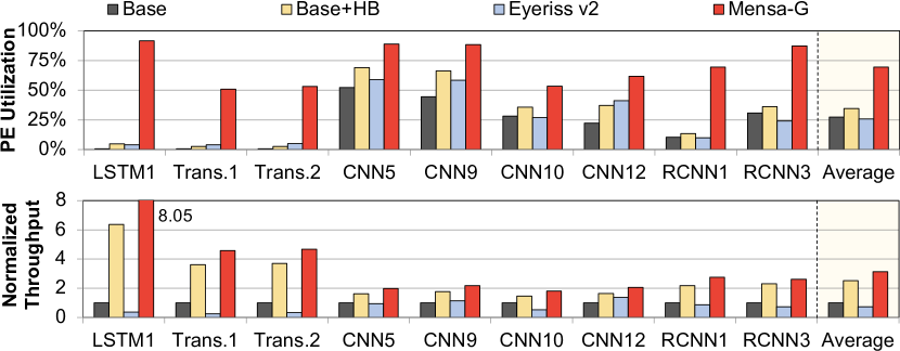
Figure 11: PE utilization (top) and Baseline-normalized throughput (bottom) across different models.

First, Baseline suffers from low PE array utilization (on average 27.3%). The higher memory bandwidth in Base+HB increases the average PE utilization to 34.0%, and improves throughput by 2.5x. The largest throughput improvements with Base+HB are for LSTMs and Transducers (4.5x on average vs. 1.3x for CNNs), thanks to their low $\mathrm{FLOP}\text{/}\mathrm{B}$ ratio and large footprints. In contrast, some CNN models (e.g., CNN10) see only modest improvements (11.7%) with Base+HB, as their layers have high reuse and small footprints. Overall, Base+HB still has very low utilization, as many layers (those from Families 3, 4, and 5) do not need the large number of PEs in the accelerator.

Second, Eyeriss v2 reduces performance significantly over Baseline for several models. Eyeriss v2’s flexible interconnect and much smaller PE array allow it to achieve slightly higher PE utilization than Baseline for layers with very low data reuse. However, this higher utilization is offset by significantly higher inference latencies. For compute-intensive layers in Families 1 and 2, the smaller PE array size hurts layer throughput. For data-intensive layers in Families 3, 4 and 5, Eyeriss v2 cannot customize its dataflow to expose reuse opportunities, and thus is greatly hurt by the high off-chip traffic (particularly for LSTMs and Transducers). Overall, we find that Eyeriss v2’s overall throughput is actually lower than Baseline for most of our models.

Third, Mensa-G significantly increases both average utilization (by 2.5x/2.0x/2.6x) and throughput (by 3.1x/1.3x/4.3x) over Baseline/Base+HB/Eyeriss v2. The large utilization improvements are a result of (1) properly-provisioned PE arrays for each layer, (2) customized dataflows that exploit reuse and opportunities for parallelization, and (3) the movement of large-footprint layer computation into 3D-stacked memory (which eliminates off-chip traffic for their DRAM requests). We note that Mensa-G’s throughput improvements over Base+HB are smaller than its utilization improvements. Even though Base+HB achieves poor energy efficiency and underutilization for layers with poor reuse and large footprints, it is reasonably effective at reducing the inference latency for such layers. Mensa-G benefits all NN model types, but the largest improvements are for LSTMs and Transducers, with average utilization/throughput improvements of 82.0x/5.7x over Baseline. The improvement is lower for CNNs and RCNNs (2.23x/1.8x over Baseline), because they make better use of Baseline’s large PE arrays, and have smaller footprints that lessen the impact of off-chip DRAM accesses. For a few CNNs (CNN10–CNN13) that use a large number of depthwise layers (which belong to Family 5), Mensa-G’s PE utilization is somewhat lower than desired (44.7%) due to the depthwise layers. These CNNs have significantly lower data reuse than other Family 4/5 layers, which in turn, makes these layers run less optimally with Jacquard’s dataflow. However, Mensa-G still improves PE utilization for depthwise layers by 65.2% over Baseline, as a result of Jacquard’s specialization.

7.3 Latency Analysis

Figure 12 shows the Baseline-normalized inference latency, and its breakdown across the three Mensa-G accelerators (Pascal, Pavlov, Jacquard). We find that Mensa-G reduces inference latency over Baseline and Base+HB on average by 1.96x and 1.17x. LSTMs and Transducers see a significant latency reduction with Mensa-G (5.4x/1.26x vs. Baseline/Base+HB) because most of their layers run on Pavlov and benefit from an optimized dataflow and processing-in-memory (which provides not only higher bandwidth, but also lower latency for DRAM accesses). CNNs and RCNNs benefit from the heterogeneity of our accelerators, making use of all three of them to reduce latency by 1.64x/1.16x over Baseline/Base+HB.

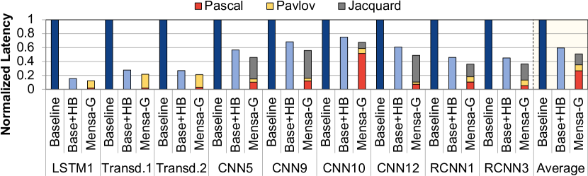
Figure 12: Inference latency, normalized to Baseline.

8 A Case for Mensa Beyond the Edge TPU

Accounting for Diversity in Other State-of-the-Art Accelerators. Our evaluation of Mensa-G shows that Mensa can significantly improve performance and energy by replacing the core of the Google Edge TPU (i.e., the PE array and interconnect) with multiple accelerators. While our characterization and analysis focus on the Google Edge TPU, the resulting insights can also be applied to several state-of-the-art accelerators that are based on systolic arrays (e.g., Eyeriss v2 [9], MAERI [60], HDA [59]). The fundamental design of these accelerators, like the Edge TPU, is centered around an array of PEs that are connected using on-chip networks to each other and to on-chip buffers. During inference, the accelerators orchestrate a specific dataflow across the interconnected PEs, buffers, and off-chip memory. Systolic-array-based accelerators deployed for edge inference will need to be designed to efficiently accommodate the very diverse behavior that we uncover across and within edge neural network models. We note that the edge models that we evaluate include (1) several models that are widely used in the community, and (2) emerging models (e.g., LSTMs, Transducers) that are expected to be of high importance in the near future. As a result, our characterization can be helpful in informing the diversity that future edge inference accelerators should capture.

Adopting Multi-Accelerator Frameworks. We believe that there is a strong case for adopting the Mensa framework for future accelerator designs. Given the tight area and energy resource budgets available for machine learning inference, it has become critical to maximize the efficiency of the accelerator hardware, even at the expense of some additional design effort. Our example implementation of Mensa for Google edge models demonstrates that we can decrease energy costs compared to a monolithic general-purpose accelerator by tailoring multiple accelerators according to the characteristics of different NN models. We believe that Mensa can work together with other existing accelerator designs beyond the Edge TPU, where Mensa manages multiple instances of the accelerator with each instance customized (at design time and/or runtime) and properly provisioned for a subset of models.

Providing Flexibility to Incorporate New NN Model Types. As our study exposes, the emergence of new model types (e.g., LSTMs, Transducers) can often demand different resource trade-offs to achieve high efficiency. With the popularity of machine learning today, we expect that new models will emerge that do not run optimally on any of our three proposed accelerators. With the Mensa framework, which uses a software-level scheduler to coordinate the mapping of layers to accelerators, we can significantly reduce design and deployment costs for new accelerators that cater to these new models. This is because Mensa’s scheduler can easily incorporate the attributes of new accelerators and identify which layers to map to them, without requiring significant changes to the runtime software.

9 Related Work

To our knowledge, this is the first work to (1) examine the bottlenecks of a state-of-the-art commercial Google Edge TPU when executing state-of-the-art Google edge neural network models; (2) quantify the significant intra- and inter-layer variation that exists in state-of-the-art edge NN models; (3) identify that layers can be clustered together based on a number of shared execution characteristics; (4) propose a new framework for heterogeneous ML inference acceleration (called Mensa), with both on-chip and near-data accelerators; and (5) provide and evaluate the performance and energy benefits of an example heterogeneous accelerator design for Google edge NN models.

Studies on a Single NN Model Type. Many prior works [85, 8, 20, 9, 17, 102, 36, 92, 91, 35, 83, 55, 1, 2, 7, 68, 73, 82] examine a specific model type (predominantly CNNs). None of these works perform an analysis across different classes of edge NN models (e.g., Transducers, LSTMs, RCNNs). In fact, many studies (e.g., [8, 20, 17, 82, 73]) analyze traditional models (e.g., AlexNet [57], VGG [86]), and their acceleration proposals are not tailored toward state-of-the-art edge NN models (which we show are different) or resource-limited edge devices. These proposals customize accelerators toward a particular model type (e.g., CNNs [8, 20, 91, 83, 73], LSTMs [85, 102]), and thus they are not optimized to serve multiple model types. As a result, they all suffer from the accelerator shortcomings we discuss in detail in Section 3.

Studies on NN Heterogeneity. Some CNN-focused works observe diversity across CNN layers [58, 92, 9, 60, 52, 82]. MAERI [60] proposes an accelerator with a reconfigurable on-chip network that connects various building blocks together. MAERI’s network can be configured to support different dataflows between PEs. Eyeriss v2 [9] includes a reconfigurable on-chip network as well, but uses a single dataflow that can support a wide range of CNN models. Despite the network reconfigurability, both MAERI and Eyeriss v2 (1) cannot customize a number of essential design parameters (e.g., off-chip memory bandwidth, on-chip memory) to different layers, (2) require frequent online reconfiguration to adapt to intra- and inter-layer variation, and (3) make it difficult to co-design the dataflow with key components such as the memory system. We compare Mensa-G to Eyeriss v2 in Section 7 and show that Mensa-G provides significantly higher performance and energy efficiency.

ScaleDeep [92] proposes customized processing tiles to address diversity in CNN layers. While the idea shares some similarities with Mensa (exploiting heterogeneity in hardware), there are two key differences. First, while Mensa targets inference using a diverse set of edge NN models (including LSTMs, Transducers), ScaleDeep targets cloud-based training of mainly traditional CNN-based models. The resource trade-offs are significantly different between the two targets: edge NN inference optimizes for tight area and energy constraints, while cloud-based training optimizes for energy efficiency and performance at very large scale. Second, due to its focus on CNNs, ScaleDeep does not address the extensive diversity that exists between CNN layers and layers in other model types (e.g., LSTM layers). Neurosurgeon [52] examines at both vision and speech models. However, their analysis is done on old/traditional vision/speech models, and their solution relies on offloading some layers to the cloud, which is counter to the goal of running inference locally and efficiently at edge devices.

Concurrent work on heterogeneous dataflow accelerators (HDA) [59] demonstrates the existence of layer-to-layer heterogeneity, and proposes a family of sub-accelerators where each sub-accelerator has a different dataflow. Our work has two key differences from HDA. First, while HDA focuses on changing accelerator dataflows, Mensa holistically considers all aspects of accelerator design (PE array, dataflow, on-chip memory, off-chip memory bandwidth) across a wider variety of state-of-the-art models. For example, with HDA, Transducers would still likely suffer from high underutilization (due to inadequate off-chip bandwidth) and very low energy efficiency (due to high off-chip parameter off-chip traffic and on-chip buffer inefficiency), while Mensa overcomes these issues. Second, HDA focuses on optimizing concurrent multi-NN execution, and does not consider the area overheads and energy efficiency goals that need to be met for edge inference (which Mensa takes into account).

10 Conclusion

We conduct the first comprehensive workload and bottleneck analysis of the Google Edge TPU, a state-of-the-art ML inference accelerator, using 24 state-of-the-art Google edge NN models including CNNs, LSTMs, Transducers, and RCNNs. Our analysis reveals that the Edge TPU’s monolithic design leads to significant underutilization and poor energy efficiency for edge NN models, which exhibit significant variation across and within NN layers. We propose (i) a new HW/SW framework called Mensa, which integrates and manages layer execution across multiple small heterogeneous accelerators, each tailored to specific layer characteristics; and (ii) a runtime scheduler for Mensa to determine which of these accelerators should execute which layer. Using our novel observation that layers from various NN models group into a small number of clusters, we create a Mensa design for the Google edge NN models consisting of three new accelerators, each of which has customized compute, memory, and dataflow characteristics. Compared to the Edge TPU, our design improves energy efficiency and throughput by 3.0x and 3.1x, while reducing inference latency by 1.96x, for the 24 state-of-the-art Google Edge NN models. Compared to a state-of-the-art reconfigurable ML accelerator (Eyeriss v2), our design improves energy efficiency by 2.4x and throughput by 4.3x for the 24 Google Edge NN models. We hope that Mensa inspires future work on NN acceleration to account for the significant heterogeneity that exists in and across NN models, and to adopt flexible frameworks such as Mensa to efficiently provide heterogeneous acceleration for both existing and yet-to-be-developed NN model types.

References

- [1] J. Albericio, P. Judd, T. Hetherington, T. Aamodt, N. Enright Jerger, and A. Moshovos, “Cnvlutin: Ineffectual-Neuron-Free Deep Neural Network Computing,” in ISCA, 2016.
- [2] M. Alwani, H. Chen, M. Ferdman, and P. Milder, “Fused-Layer CNN Accelerators,” in MICRO, 2016.
- [3] A. Boroumand, S. Ghose, M. Patel, H. Hassan, B. Lucia, K. Hsieh, K. T. Malladi, H. Zheng, and O. Mutlu, “LazyPIM: An Efficient Cache Coherence Mechanism for Processing-in-Memory,” IEEE CAL, 2017.
- [4] A. Boroumand, S. Ghose, Y. Kim, R. Ausavarungnirun, E. Shiu, R. Thakur, D. Kim, A. Kuusela, A. Knies, P. Ranganathan, and O. Mutlu, “Google Workloads for Consumer Devices: Mitigating Data Movement Bottlenecks,” in ASPLOS, 2018.
- [5] A. Boroumand, S. Ghose, M. Patel, H. Hassan, B. Lucia, R. Ausavarungnirun, K. Hsieh, N. Hajinazar, K. T. Malladi, H. Zheng, and O. Mutlu, “CoNDA: Efficient Cache Coherence Support for Near-data Accelerators,” in ISCA, 2019.
- [6] E. Çakır, G. Parascandolo, T. Heittola, H. Huttunen, and T. Virtanen, “Convolutional Recurrent Neural Networks for Polyphonic Sound Event Detection,” TASLP, 2017.
- [7] T. Chen, Z. Du, N. Sun, J. Wang, C. Wu, Y. Chen, and O. Temam, “DianNao: A Small-Footprint High-Throughput Accelerator for Ubiquitous Machine-Learning,” in ASPLOS, 2014.
- [8] Y.-H. Chen, T. Krishna, J. S. Emer, and V. Sze, “Eyeriss: An Energy-Efficient Reconfigurable Accelerator for Deep Convolutional Neural Networks,” JSSC, 2017.
- [9] Y.-H. Chen, T. Yang, J. S. Emer, and V. Sze, “Eyeriss v2: A Flexible Accelerator for Emerging Deep Neural Networks on Mobile Devices,” JETCAS, 2019.
- [10] K. Cho, B. Van Merriënboer, D. Bahdanau, and Y. Bengio, “On the Properties of Neural Machine Translation: Encoder–Decoder Approaches,” arXiv:1409.1259 [cs.CL], 2014.
- [11] K. Cho, B. Van Merriënboer, C. Gulcehre, D. Bahdanau, F. Bougares, H. Schwenk, and Y. Bengio, “Learning Phrase Representations Using RNN Encoder-Decoder for Statistical Machine Translation,” arXiv:1406.1078 [cs.CL], 2014.
- [12] J. W. Choi, D. Bedard, R. Fowler, and R. Vuduc, “A Roofline Model of Energy,” in IPDPS, 2013.
- [13] K. Choi, G. Fazekas, M. Sandler, and K. Cho, “Convolutional Recurrent Neural Networks for Music Classification,” in ICASSP, 2017.
- [14] J. Chung, C. Gulcehre, K. Cho, and Y. Bengio, “Empirical Evaluation of Gated Recurrent Neural Networks on Sequence Modeling,” in NeurIPS, 2014.
- [15] J. Donahue, L. A. Hendricks, S. Guadarrama, M. Rohrbach, S. Venugopalan, K. Saenko, and T. Darrell, “Long-Term Recurrent Convolutional Networks for Visual Recognition and Description,” in CVPR, 2015.
- [16] M. Drumond, A. Daglis, N. Mirzadeh, D. Ustiugov, J. Picorel, B. Falsafi, B. Grot, and D. Pnevmatikatos, “The Mondrian Data Engine,” in ISCA, 2017.
- [17] Z. Du, R. Fasthuber, T. Chen, P. Ienne, L. Li, T. Luo, X. Feng, Y. Chen, and O. Temam, “ShiDianNao: Shifting Vision Processing Closer to the Sensor,” in ISCA, 2015.
- [18] J. Fowers, K. Ovtcharov, M. Papamichael, T. Massengill, M. Liu, D. Lo, S. Alkalay, M. Haselman, L. Adams, M. Ghandi, S. Heil, P. Patel, A. Sapek, G. Weisz, L. Woods, S. Lanka, S. K. Reinhardt, A. M. Caulfield, E. S. Chung, and D. Burger, “A Configurable Cloud-Scale DNN Processor for Real-Time AI,” in ISCA, 2018.
- [19] K. Fukushima, “Neocognitron: A Self-Organizing Neural Network Model for a Mechanism of Pattern Recognition Unaffected by Shift in Position,” Biological Cybernetics, 1980.
- [20] M. Gao, J. Pu, X. Yang, M. Horowitz, and C. Kozyrakis, “TETRIS: Scalable and Efficient Neural Network Acceleration with 3D Memory,” in ASPLOS, 2017.
- [21] M. Gao, X. Yang, J. Pu, M. Horowitz, and C. Kozyrakis, “TANGRAM: Optimized Coarse-Grained Dataflow for Scalable NN Accelerators,” in ASPLOS, 2019.
- [22] F. Gers, J. Schmidhuber, and F. Cummins, “Learning to Forget: Continual Prediction with LSTM,” in ICANN, 1999.
- [23] S. Ghose, K. Hsieh, A. Boroumand, R. Ausavarungnirun, and O. Mutlu, “Enabling the Adoption of Processing-in-Memory: Challenges, Mechanisms, Future Research Directions,” arxiv:1802.00320 [cs.AR], 2018.
- [24] S. Ghose, K. Hsieh, A. Boroumand, R. Ausavarungnirun, and O. Mutlu, “The Processing-in-Memory Paradigm: Mechanisms to Enable Adoption,” in Beyond-CMOS Technologies for Next Generation Computer Design, 2019.
- [25] P. Gibson, J. Cano, J. Turner, E. J. Crowley, M. O’Boyle, and A. Storkey, “Optimizing Grouped Convolutions on Edge Devices,” in ASAP, 2020.
- [26] Google LLC, “Edge TPU,” https://cloud.google.com/edge-tpu/.
- [27] Google LLC, “Edge TPU Compiler,” https://coral.ai/docs/edgetpu/compiler/.
- [28] Google LLC, “TensorFlow Lite,” https://www.tensorflow.org/lite/.
- [29] Google LLC, “TensorFlow Models on the Edge TPU,” https://coral.ai/docs/edgetpu/models-intro/.
- [30] A. Graves, “Sequence Transduction with Recurrent Neural Networks,” in ICML Representation Workshop, 2012, arXiv:1211.3711 [cs.NE].
- [31] A. Graves, “Generating Sequences with Recurrent Neural Networks,” arXiv:1308.0850 [cs.NE], 2013.
- [32] A. Graves, N. Jaitly, and A.-r. Mohamed, “Hybrid Speech Recognition with Deep Bidirectional LSTM,” in ASRU, 2013.
- [33] K. Greff, R. K. Srivastava, J. Koutník, B. R. Steunebrink, and J. Schmidhuber, “LSTM: A Search Space Odyssey,” TNNLS, 2017.
- [34] J. Gu, Z. Wang, J. Kuen, L. Ma, A. Shahroudy, B. Shuai, T. Liu, X. Wang, G. Wang, J. Cai, and T. Chen, “Recent Advances in Convolutional Neural Networks,” Pattern Recognition, 2018.
- [35] S. Gudaparthi, S. Narayanan, R. Balasubramonian, E. Giacomin, H. Kambalasubramanyam, and P.-E. Gaillardon, “Wire-Aware Architecture and Dataflow for CNN Accelerators,” in MICRO, 2019.
- [36] U. Gupta, B. Reagen, L. Pentecost, M. Donato, T. Tambe, A. M. Rush, G. Wei, and D. Brooks, “MASR: A Modular Accelerator for Sparse RNNs,” in PACT, 2019.
- [37] S. Han, J. Kang, H. Mao, Y. Hu, X. Li, Y. Li, D. Xie, H. Luo, S. Yao, Y. Wang, H. Yang, and W. J. Dally, “ESE: Efficient Speech Recognition Engine with Sparse LSTM on FPGA,” in FPGA, 2017.
- [38] K. He, X. Zhang, S. Ren, and J. Sun, “Deep Residual Learning for Image Recognition,” in CVPR, 2016.
- [39] Y. He, T. N. Sainath, R. Prabhavalkar, I. McGraw, R. Alvarez, D. Zhao, D. Rybach, A. Kannan, Y. Wu, R. Pang, Q. Liang, D. Bhatia, Y. Shangguan, B. Li, G. Pundak, K. C. Sim, T. Bagby, S. yiin Chang, K. Rao, and A. Gruenstein, “Streaming End-to-End Speech Recognition for Mobile Devices,” in ICASSP, 2019.
- [40] S. Hochreiter and J. Schmidhuber, “Long Short-Term Memory,” NECO, 1997.
- [41] A. G. Howard, M. Zhu, B. Chen, D. Kalenichenko, W. Wang, T. Weyand, M. Andreetto, and H. Adam, “MobileNets: Efficient Convolutional Neural Networks for Mobile Vision Applications,” arXiv:1704.04861 [cs.CV], 2017.
- [42] K. Hsieh, G. Ananthanarayanan, P. Bodik, S. Venkataraman, P. Bahl, M. Philipose, P. B. Gibbons, and O. Mutlu, “Focus: Querying Large Video Datasets with Low Latency and Low Cost,” in OSDI, 2018.
- [43] Hybrid Memory Cube Consortium, “HMC Specification 2.0,” 2014.
- [44] F. N. Iandola, S. Han, M. W. Moskewicz, K. Ashraf, W. J. Dally, and K. Keutzer, “SqueezeNet: AlexNet-Level Accuracy With 50x Fewer Parameters and 0.5MB Model Size,” arXiv:1602.07360 [cs.CV], 2016.
- [45] Intel Corp., “Intel Movidius Neural Compute Stick,” https://software.intel.com/content/www/us/en/develop/articles/intel-movidius-neural-compute-stick.html.
- [46] M. H. Ionica and D. Gregg, “The Movidius Myriad Architecture’s Potential for Scientific Computing,” IEEE Micro, 2015.
- [47] JEDEC Solid State Technology Assn., “JESD235B: High Bandwidth Memory (HBM) DRAM,” December 2018.
- [48] JEDEC Solid State Technology Assn., “JESD209-4C: Low Power Double Data Rate 4 (LPDDR4) Standard,” January 2020.
- [49] H. Jiang and E. Learned-Miller, “Face Detection with the Faster R-CNN,” in FG, 2017.
- [50] N. P. Jouppi, C. Young, N. Patil, D. Patterson, G. Agrawal, R. Bajwa, S. Bates, S. Bhatia, N. Boden, A. Borchers, R. Boyle, P. luc Cantin, C. Chao, C. Clark, J. Coriell, M. Daley, M. Dau, J. Dean, B. Gelb, T. V. Ghaemmaghami, R. Gottipati, W. Gulland, R. Hagmann, C. R. Ho, D. Hogberg, J. Hu, R. Hundt, D. Hurt, J. Ibarz, A. Jaffey, A. Jaworski, A. Kaplan, H. Khaitan, A. Koch, N. Kumar, S. Lacy, J. Laudon, J. Law, D. Le, C. Leary, Z. Liu, K. Lucke, A. Lundin, G. MacKean, A. Maggiore, M. Mahony, K. Miller, R. Nagarajan, R. Narayanaswami, R. Ni, K. Nix, T. Norrie, M. Omernick, N. Penukonda, A. Phelps, J. Ross, M. Ross, A. Salek, E. Samadiani, C. Severn, G. Sizikov, M. Snelham, J. Souter, D. Steinberg, A. Swing, M. Tan, G. Thorson, B. Tian, H. Toma, E. Tuttle, V. Vasudevan, R. Walter, W. Wang, E. Wilcox, and D. H. Yoon, “In-Datacenter Performance Analysis of a Tensor Processing Unit,” in ISCA, 2017.
- [51] S. Kanai, Y. Fujiwara, and S. Iwamura, “Preventing Gradient Explosions in Gated Recurrent Units,” in NeurIPS, 2017.
- [52] Y. Kang, J. Hauswald, C. Gao, A. Rovinski, T. Mudge, J. Mars, and L. Tang, “Neurosurgeon: Collaborative Intelligence Between the Cloud and Mobile Edge,” in ASPLOS, 2017.
- [53] A. Kannan, K. Kurach, S. Ravi, T. Kaufmann, A. Tomkins, B. Miklo, G. Corrado, L. Lukács, M. Ganea, P. Young, and V. Ramavajjala, “Smart Reply: Automated Response Suggestion for Email,” in KDD, 2016.
- [54] A. Karpathy and L. Fei-Fei, “Deep Visual-Semantic Alignments for Generating Image Descriptions,” in CVPR, 2015.
- [55] L. Ke, U. Gupta, B. Y. Cho, D. Brooks, V. Chandra, U. Diril, A. Firoozshahian, K. Hazelwood, B. Jia, H. S. Lee, M. Li, B. Maher, D. Mudigere, M. Naumov, M. Schatz, M. Smelyanskiy, X. Wang, B. Reagen, C. Wu, M. Hempstead, and X. Zhang, “RecNMP: Accelerating Personalized Recommendation with Near-Memory Processing,” in ISCA, 2020.
- [56] A. Khamparia, B. Pandey, S. Tiwari, D. Gupta, A. Khanna, and J. Rodrigues, “An Integrated Hybrid CNN–RNN Model for Visual Description and Generation of Captions,” CSSP, 2019.
- [57] A. Krizhevsky, I. Sutskever, and G. E. Hinton, “ImageNet Classification with Deep Convolutional Neural Networks,” CACM, 2017.
- [58] H. Kwon, P. Chatarasi, M. Pellauer, A. Parashar, V. Sarkar, and T. Krishna, “Understanding Reuse, Performance, and Hardware Cost of DNN Dataflow: A Data-Centric Approach,” in MICRO, 2019.
- [59] H. Kwon, L. Lai, M. Pellauer, T. Krishna, Y.-H. Chen, and V. Chandra, “Heterogeneous Dataflow Accelerators for Multi-DNN Workloads,” in HPCA, 2021.
- [60] H. Kwon, A. Samajdar, and T. Krishna, “MAERI: Enabling Flexible Dataflow Mapping over DNN Accelerators via Reconfigurable Interconnects,” in ASPLOS, 2018.
- [61] Y. LeCun, “Une Procédure d’Apprentissage pour Réseau à Seuil Asymétrique,” in Cognitiva, 1985.
- [62] Y. LeCun, Y. Bengio, and G. Hinton, “Deep Learning,” Nature, 2015.
- [63] Y. LeCun, B. Boser, J. Denker, D. Henderson, R. Howard, W. Hubbard, and L. Jackel, “Handwritten Digit Recognition with a Back-Propagation Network,” in NeurIPS, 1989.
- [64] Y. LeCun, L. Bottou, Y. Bengio, and P. Haffner, “Gradient-Based Learning Applied to Document Recognition,” Proc. IEEE, 1998.
- [65] H. Li, Z. Lin, X. Shen, J. Brandt, and G. Hua, “A Convolutional Neural Network Cascade for Face Detection,” in CVPR, 2015.
- [66] J. Li, R. Zhao, H. Hu, and Y. Gong, “Improving RNN Transducer Modeling for End-to-End Speech Recognition,” in ASRU, 2019.
- [67] M. Liang and X. Hu, “Recurrent Convolutional Neural Network for Object Recognition,” in CVPR, 2015.
- [68] W. Lu, G. Yan, J. Li, S. Gong, Y. Han, and X. Li, “FlexFlow: A Flexible Dataflow Accelerator Architecture for Convolutional Neural Networks,” in HPCA, 2017.
- [69] N. Ma, X. Zhang, H.-T. Zheng, and J. Sun, “ShuffleNet V2: Practical Guidelines for Efficient CNN Architecture Design,” in ECCV, 2018.
- [70] N. Muralimanohar, R. Balasubramonian, and N. Jouppi, “Optimizing NUCA Organizations and Wiring Alternatives for Large Caches with CACTI 6.0,” in MICRO, 2007.
- [71] O. Mutlu, S. Ghose, J. Gomez-Luna, and R. Ausavarungnirun, “Processing Data Where It Makes Sense: Enabling In-Memory Computation,” MICPRO, 2019.
- [72] NVIDIA Corp., “NVIDIA Jetson Nano,” https://developer.nvidia.com/embedded/jetson-nano-developer-kit.
- [73] A. Parashar, M. Rhu, A. Mukkara, A. Puglielli, R. Venkatesan, B. Khailany, J. Emer, S. W. Keckler, and W. J. Dally, “SCNN: An Accelerator for Compressed-Sparse Convolutional Neural Networks,” in ISCA, 2017.
- [74] P. Pinheiro and R. Collobert, “Recurrent Convolutional Neural Networks for Scene Labeling,” in ICML, 2014.
- [75] H. Qin, J. Yan, X. Li, and X. Hu, “Joint Training of Cascaded CNN for Face Detection,” in CVPR, 2016.
- [76] M. Ranzato, A. Szlam, J. Bruna, M. Mathieu, R. Collobert, and S. Chopra, “Video (Language) Modeling: A Baseline for Generative Models of Natural Videos,” arXiv:1412.6604 [cs.LG], 2014.
- [77] K. Rao, H. Sak, and R. Prabhavalkar, “Exploring Architectures, Data and Units for Streaming End-to-End Speech Recognition with RNN-Transducer,” arXiv:1801.00841 [cs.CL], 2018.
- [78] C. Rui, X. Wang, W. Zhang, X. Zhu, A. Li, and C. Yang, “A Hybrid CNN–LSTM Model for Typhoon Formation Forecasting,” GeoInformatica, 2019.
- [79] D. Rumelhart, G. E. Hinton, and R. J. Williams, “Learning Representations by Back-Propagating Errors,” Nature, 1986.
- [80] O. Russakovsky, J. Deng, H. Su, J. Krause, S. Satheesh, S. Ma, Z. Huang, A. Karpathy, A. Khosla, M. Bernstein et al., “ImageNet Large Scale Visual Recognition Challenge,” IJCV, 2015.
- [81] H. Sak, A. W. Senior, and F. Beaufays, “Long Short-Term Memory Based Recurrent Neural Network Architectures for Large Vocabulary Speech Recognition,” arXiv:1402.1128 [cs.NE], 2014.
- [82] Y. S. Shao, J. Clemons, R. Venkatesan, B. Zimmer, M. Fojtik, N. Jiang, B. Keller, A. Klinefelter, N. Pinckney, P. Raina, S. G. Tell, Y. Zhang, W. J. Dally, J. Emer, C. T. Gray, B. Khailany, and S. W. Keckler, “Simba: Scaling Deep-Learning Inference with Multi-Chip-Module-Based Architecture,” in MICRO, 2019.
- [83] Y. Shen, M. Ferdman, and P. Milder, “Maximizing CNN Accelerator Efficiency Through Resource Partitioning,” in ISCA, 2017.
- [84] D. Shin, J. Lee, J. Lee, and H. Yoo, “DNPU: An 8.1TOPS/W Reconfigurable CNN–RNN Processor for General-Purpose Deep Neural Networks,” in ISSCC, 2017.
- [85] F. Silfa, G. Dot, J.-M. Arnau, and A. González, “E-PUR: An Energy-Efficient Processing Unit for Recurrent Neural Networks,” in PACT, 2018.
- [86] K. Simonyan and A. Zisserman, “Very Deep Convolutional Networks for Large-Scale Image Recognition,” in ICLR, 2015.
- [87] H. Soltau, H. Liao, and H. Sak, “Neural Speech Recognizer: Acoustic-to-Word LSTM Model for Large Vocabulary Speech Recognition,” arXiv:1610.09975 [cs.CL], 2016.
- [88] N. Srivastava, E. Mansimov, and R. Salakhudinov, “Unsupervised Learning of Video Representations Using LSTMs,” in ICML, 2015.
- [89] I. Sutskever, O. Vinyals, and Q. V. Le, “Sequence to Sequence Learning with Neural Networks,” in NeurIPS, 2014.
- [90] C. Szegedy, W. Liu, Y. Jia, P. Sermanet, S. Reed, D. Anguelov, D. Erhan, V. Vanhoucke, and A. Rabinovich, “Going Deeper with Convolutions,” in CVPR, 2015.
- [91] F. Tu, W. Wu, S. Yin, L. Liu, and S. Wei, “RANA: Towards Efficient Neural Acceleration with Refresh-Optimized Embedded DRAM,” in ISCA, 2018.
- [92] S. Venkataramani, A. Ranjan, S. Banerjee, D. Das, S. Avancha, A. Jagannathan, A. Durg, D. Nagaraj, B. Kaul, P. Dubey, and A. Raghunathan, “ScaleDeep: A Scalable Compute Architecture for Learning and Evaluating Deep Networks,” in ISCA, 2017.
- [93] O. Vinyals, A. Toshev, S. Bengio, and D. Erhan, “Show and Tell: A Neural Image Caption Generator,” in CVPR, 2015.
- [94] C. Wu, D. Brooks, K. Chen, D. Chen, S. Choudhury, M. Dukhan, K. Hazelwood, E. Isaac, Y. Jia, B. Jia, T. Leyvand, H. Lu, Y. Lu, L. Qiao, B. Reagen, J. Spisak, F. Sun, A. Tulloch, P. Vajda, X. Wang, Y. Wang, B. Wasti, Y. Wu, R. Xian, S. Yoo, and P. Zhang, “Machine Learning at Facebook: Understanding Inference at the Edge,” in HPCA, 2019.
- [95] Y. Wu, M. Schuster, Z. Chen, Q. V. Le, M. Norouzi, W. Macherey, M. Krikun, Y. Cao, Q. Gao, K. Macherey, J. Klingner, A. Shah, M. Johnson, X. Liu, L. Kaiser, S. Gouws, Y. Kato, T. Kudo, H. Kazawa, K. Stevens, G. Kurian, N. Patil, W. Wang, C. Young, J. Smith, J. Riesa, A. Rudnick, O. Vinyals, G. S. Corrado, M. Hughes, and J. Dean, “Google’s Neural Machine Translation System: Bridging the Gap Between Human and Machine Translation,” arXiv:1609.08144 [cs.CL], 2016.
- [96] S. Xingjian, Z. Chen, H. Wang, D.-Y. Yeung, W.-K. Wong, and W.-c. Woo, “Convolutional LSTM Network: A Machine Learning Approach for Precipitation Nowcasting,” in NeurIPS, 2015.
- [97] K. Xu, J. Ba, R. Kiros, K. Cho, A. Courville, R. Salakhudinov, R. Zemel, and Y. Bengio, “Show, Attend and Tell: Neural Image Caption Generation with Visual Attention,” in ICML, 2015.
- [98] X. Xu, Y. Ding, S. X. Hu, M. T. Niemier, J. Cong, Y. Hu, and Y. Shi, “Scaling for Edge Inference of Deep Neural Networks,” Nature Electronics, 2018.
- [99] M. D. Zeiler and R. Fergus, “Visualizing and Understanding Convolutional Networks,” in ECCV, 2014.
- [100] X. Zhang, X. Liu, A. Ramachandran, C. Zhuge, S. Tang, P. Ouyang, Z. Cheng, K. Rupnow, and D. Chen, “High-Performance Video Content Recognition with Long-Term Recurrent Convolutional Network for FPGA,” in FPL, 2017.
- [101] X. Zhang, X. Zhou, M. Lin, and J. Sun, “ShuffleNet: An Extremely Efficient Convolutional Neural Network for Mobile Devices,” in CVPR, 2018.
- [102] T. Zhao, Y. Zhang, and K. Olukotun, “Serving Recurrent Neural Networks Efficiently with a Spatial Accelerator,” arXiv:1909.13654 [cs.DC], 2019.
- [103] Z. Zhao, W. Chen, X. Wu, P. C. Y. Chen, and J. Liu, “LSTM Network: A Deep Learning Approach for Short-Term Traffic Forecast,” IET ITS, 2017.