Theoretical estimate of the half-life for the radioactive ¹³⁴Cs and ¹³⁵Cs in astrophysical scenarios

Abstract

We analyze the ${}^{134}_{55}$Cs$\rightarrow^{134}_{56}$Ba and ${}^{135}_{55}$Cs$\rightarrow^{135}_{56}$Ba $\beta^{-}$ decays, which are crucial production channels for Ba isotopes in Asymptotic Giant Branch (AGB) stars. We reckon, from relativistic quantum mechanis, the effects of multichannel scattering onto weak decays, including nuclear and electronic excited states (ES) populated above $\simeq$ 10 keV, for both parent and daughter nuclei. We find increases in the half-lives for $T>10^{8}$ K (by more than a factor 3 for ¹³⁴Cs) as compared to previous works based on systematics. We also discuss our method in view of these previous calculations. An important impact on half-lives comes from nuclear ES decays, while including electronic temperatures yields further increases of about 20% at energies 10-30 keV, typical of AGB stars of moderate mass ($M\lesssim 8~{}M_{\odot}$). Despite properly considering these effects, the new rates remain sensitively lower than the TY values, implying longer half-lives at least above 8-9 keV. Our rate predictions are in substantial accord with recent results based on the shell model, and strongly modify branching ratios along the $s$-process path previously adopted. With our new rate, nucleosynthesis models well account for the isotopic admixtures of Ba in presolar SiC grains and in the Sun.

1 Introduction

New scenarios to unravel heavy-element nucleosynthesis in stars were recently opened by extended surveys of spectroscopic observations (Ahumada & et al., 2020), as well as by the analysis of presolar grains formed in stellar winds, which were trapped in pristine meteorites (Palmerini et al., 2021), offering new constraints on the isotopic abundances generated in stellar processes (Busso et al., 2021).

After decades of experiments on reaction-rates for neutron-captures and charged-particle processes, our understanding of the above scenario now depends also on improving the knowledge of weak nuclear reactions in hot stellar plasmas. Their accurate assessment still represents a crucial bottleneck, while experiments simulating stellar conditions in terrestrial ionized plasmas to measure decay rates are still in their infancy (Mascali et al., 2017, 2022). In particular, for a better agreement between nucleosynthesis models and observations (Vescovi et al., 2019) a great deal of theoretical work to assess stellar reaction rates with increased accuracy is still required (Nomoto et al., 2013); in fact, there is a dearth of computations for decay processes in stellar scenarios from first-principles (Simonucci et al., 2013; Vescovi et al., 2019).

In this respect, we notice that $\beta$-decay spectra of allowed and forbidden transitions are typically calculated by using an analytical expression of the rate (Hayen et al., 2018), where semi-empirical factors account for the nuclear structure, the phase-space, and the atomic exchange. However, not even this simpler approach is implemented in stellar neutron capture computations, where, instead, the phenomenological compilation (Takahashi & Yokoi, 1983, 1987) (hereafter TY) is universally used. There, unknown transition strengths are estimated by analogy to laboratory decays of nearby nuclei with similar transitions. In a recent study for example (Li et al., 2021), new $\log(ft)$ values were calculated from the nuclear shell model to obtain ¹³⁴Cs stellar rates within this standard approach (Hayen et al., 2018). In this work the electronic degree of freedom (DOF) is neglected, despite its crucial contribution to the rate. Nevertheless, the authors already show significant improvement in the astrophysical application, with the rate changing in the same direction as found using our analysis. Recently developed approaches, based on large-scale diagonalization shell model calculations, can be also used (Langanke et al., 2021), even though they have seen so far applications only to part of the nuclide chart.

One element requiring such studies is certainly Barium. In AGB stars, its abundance depends solely on slow ($s$) process nucleosynthesis that after the $n$-capture on stable ¹³³Cs meets a branching point at ¹³⁴Cs, where further $n$-captures compete with $\beta$-decay, e.g. the ${}_{55}^{134}\mathrm{Cs}(J^{\pi}=4^{+})\longrightarrow_{56}^{134}\mathrm{Ba}(J^{\pi}=4^{+})+e^{-}+\bar{\nu}$ allowed transition. Another reaction branching occurs at ¹³⁵Cs, $\beta$-decaying to ¹³⁵Ba via a 2^nd forbidden unique transition Cs$(7/2^{+})\longrightarrow$ Ba$(3/2^{+})$. The resulting balance, which should yield production of 100% of the $s$-only ¹³⁴Ba and ¹³⁶Ba isotopes, is thus very delicate. In particular, the ¹³⁴Cs $\longrightarrow^{134}$Ba decay (half-life 2.0652 y) is characterized by a Q-value (2058.7 keV; Sonzogni 2004) large enough to accommodate Cs high-lying nuclear excited states (ESs), e.g. $5^{+}$ at 11.2442 keV and $3^{+}$ at 60 keV above the ground state (GS). The emergence of ¹³⁴Cs short-lived nuclear ESs, possibly populated at high temperature, and the decay to ¹³⁴Ba isomers (such as $4^{+}$, $3^{+}$) may dramatically affect this transition owing to their different forbiddenness.

When $n$-capture on ¹³⁴Cs feeds the longer-lived ¹³⁵Cs, also the latter can decay through the mentioned Cs$(7/2^{+})\longrightarrow$ Ba$(3/2^{+})$ path. Its half-life is $2.3\times 10^{6}$ y (with a GS-GS $Q$-value of 268.7 keV; Singh et al. 2008). The inclusion of several ES of ¹³⁵Cs (notably the $5/2^{+}$ states at 249.767 and 408.026 keV above the GS), together with the population of electronic excited levels, may significantly affect the total rate at high temperature also for this nucleus.

Furthermore, despite these transitions being quark-level processes, they also strongly depend on extra-nuclear factors, such as temperature and electron density, which significantly vary in the layers of evolved stars outside the degenerate core. Indeed, these parameters may affect the ionization degree of the atomic systems where the decay occurs, which in turn modifies the discrete–to–continuum transition ratio (Simonucci et al., 2013; Palmerini et al., 2016; Vescovi et al., 2019).

In this work we lay the foundation of a fully-relativistic quantum-mechanical method for calculating the temperature and density dependence of the $\beta$-decay half-life of s-process branching point isotopes, by considering both the electronic and nuclear ES population dynamics, and apply it here for the first time to ¹³⁴Cs and ¹³⁵Cs. We show that these DOFs act concurrently to strongly change the Cs isotopes half-lives, even by several orders of magnitude, with respect to laboratory conditions and previous phenomenological approaches based on systematics (see TY). We apply this approach to revise recent models aiming to explain the peculiar ratios of Ba isotopes in presolar SiC grains and the s-process origin of the ¹³⁴Ba and ¹³⁶Ba isotopes in the solar system (Palmerini et al., 2021; Busso et al., 2021).

2 Calculation of $\beta$-decay rates of ¹³⁴Cs and ¹³⁵Cs

Our method is rooted in the single-particle mean-field (MF) approximation to the internuclear and interelectronic interactions, but is systematically and straightforwardly improvable by embedding higher accuracy many-body methods for including dynamical correlation (Hjorth-Jensen et al., 2017).

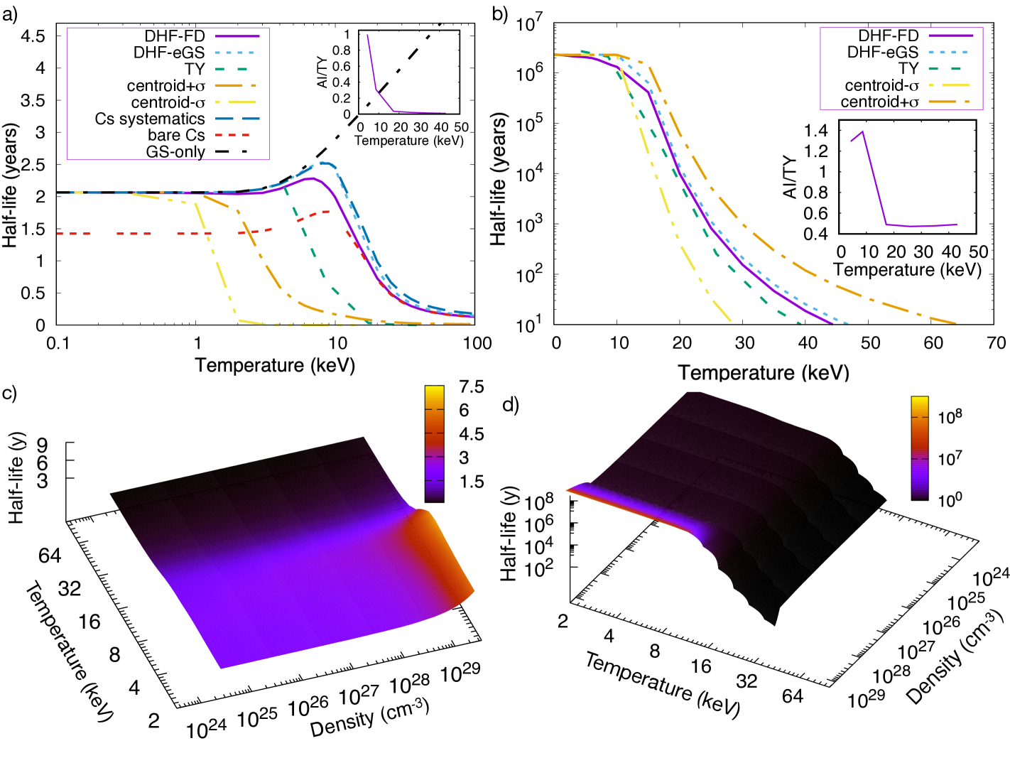
Figure 1: Half-life of ¹³⁴Cs (a) and of ¹³⁵Cs (b) vs. temperature (violet line) from our DHF calculations, for $n_{p}=10^{26}$ cm^-3. They include: (a) the nuclear states at $4^{+},5^{+},3^{+}$ of ¹³⁴Cs and (b) those of ¹³⁵Cs at $5/2^{+},5/2^{+}$, as well as the electronic DOF. In cyan (DHF-eGS) we show the half-life computed when electrons are clamped in their GS. Orange and yellow lines show the maximum (centroid+$\sigma$) and minimum (centroid-$\sigma$) values obtained by taking the $\log(ft)$ from the general systematics, while in the blue line we used simply the centroid of the specific ¹³⁴Cs systematics (this does not exist for ¹³⁵Cs). Green lines show the previous estimates by TY. In panel a) we also show (red line) the half-life for a completely ionized ¹³⁴Cs (bare Cs) and the nuclear GS to GS decay half-life (black line, GS-only). The trend is similar for ¹³⁵Cs (not shown). Insets of a) and b) give the ratios between our ab-initio rates (AI) and TY values for $n_{p}=10^{26}$ cm^-3. Panels c) and d) display ¹³⁴Cs and ¹³⁵Cs half-lives according to our model, including both nuclear and electronic DOFs, as a function of temperature and proton density.

Our approach, based on the first-principle calculation of the transition operator written in terms of the total QED Hamiltonian, proved accurate in reproducing a few terrestrial observables (Morresi et al., 2018). Here is generalized to include the temperature and density dependence for dealing with astrophysical conditions (see Appendix A for further details). Within our framework, the weak Hamiltonian is factorized into the product of leptonic and hadronic currents (Morresi et al., 2018). We also require that the hadronic current is separable into neutron and proton field operators, which means essentially that the decaying neutron acts as a single-particle correlated to the core of the remaining nucleons only geometrically, so as to recover the experimental total angular momentum of the parent reactant. Furthermore, one can safely assume that the leptonic current can be written as a product of the neutrino and electron quantum field operators. The hadronic and leptonic currents are both reckoned by the self-consistent numerical solution of the Dirac–Hartree–Fock equation (DHF).

Protons and neutrons are interacting via a semi-empirical relativistic Wood-Saxon potential, while the electron-electron Coulomb repulsion is modelled via a local density approximation to the electron gas ($V_{ex}\propto\rho(r)^{1/3}$) (Slater, 1951; Salvat et al., 1987). Electrons populate the energy levels according to a Fermi-Dirac distribution, and the chemical potential is assessed by assuming that they behave as an ideal Fermi gas in a box with a relativistic energy-momentum dispersion. The non-orthogonality between the bound initial and final orbitals, the possible presence of shake-up (excitation) and shake-off (ejection) are also taken into account in the calculation of the continuum electron wavefunction. At high temperature, we considered positron formation, enforcing the overall neutrality of the plasma (see Table 3 reporting electron vs. proton densities at all temperatures). For the ${}_{55}^{134}\mathrm{Cs}\longrightarrow_{56}^{134}\mathrm{Ba}$ transition, the lepton field carries no angular momentum. The rate has been assessed under the assumption, derived by the nuclear shell model, that the decaying neutron within the parent ¹³⁴Cs occupies the $2d_{3/2}$ shell, while the generated proton populates the $1g_{7/2}$ orbital of ${}^{134}_{56}$Ba. In principle, a superposition of single-particle near-by energy states mixed by the dynamical correlation, such as the ¹³⁴Cs $1h_{11/2}$ and $3s_{1/2}$ shells, may contribute to the $\beta$ transition. However, owing to a bigger jump of $\Delta J$ the level of forbiddenness of the $\beta$ transition from those shells to the ¹³⁴Ba $1g_{7/2}$ shell would be higher and, thus, the transition less likely to occur.

In our calculations we included the $4^{+}$ GS and the two lowest energy nuclear states ($5^{+},3^{+}$) of ¹³⁴Cs, occupied according to a Boltzmann distribution $f(E_{i})=w_{i}e^{-E_{i}/K_{\text{B}}T}$, where $E_{i}$ is the energy of the $i$-th nuclear level, weighted by the relevant level degeneration factor ($w_{i}=9,11,7$, respectively for the 3 states mentioned above).

To reproduce the experimental values at Earth conditions a constant correction factor of 4.4 to our calculated half-lives is applied at all temperatures. This renormalization factor is needed to correct the hadronic current, which may suffer from the MF evaluation of the nucleon wavefunctions. In our analysis we assume that the nuclear matrix elements do not depend on the temperature for a given transition because of the leptonic and hadronic currents factorization and of the independence of the single-particle orbitals of temperature. Indeed, the matrix elements of the hadronic currents only depend on the nuclear single-particle orbitals of the decaying neutron and of the proton before and after the decay, respectively. Once the initial parent and final daughter states are selected the hadronic current matrix elements are independent of temperature, and their energy scale (MeV) is rather different from those typical of AGB stars (keV). In light of these considerations in place, we can safely state that the correction factor is the same at all temperatures and the fact that terrestrial decays are determined by decay of atomic Cs does not play any role. The half-lives of ¹³⁴Cs with and without the correction factors are reported in Tab. 6 of the appendix B.

Table 1: Comparison between the ¹³⁴Cs rates obtained by TY and using our model (units in $s^{-1}\times 10^{-8}$) for different temperatures and fixed proton density $n_{p}=10^{26}$ cm^-3. Note that our rate remains always lower than TY suggest.

$T_{8}$	TY	This work
0.5 (4.31)	1.02	1.02
1 (8.62)	3.28	1.01
2 (17.23)	63.1	2.28
3 (25.85)	211.0	4.73
4 (34.47)	481.0	7.22
5 (43.09)	889.0	9.36

Note. — $T_{8}$ is the temperature expressed in $10^{8}$ K, while the corresponding values in keV are in parentheses.

In Fig. 1a and in the relevant inset as well as in Table 1 we compare our results with those by TY. A finer grid of points can be found in Table 4 of the appendix B. We stress that in TY the effect of the excited nuclear dynamics on the $\beta$ rates was estimated via the $\log(ft)$ values for general $\beta$ transitions of given forbiddenness derived from systematics. Moreover, at odds with our calculations, neither TY include in their estimate the electronic DOF nor they calculate the nuclear matrix elements from first-principles.

We observe that the inclusion of the nuclear ES dynamics represents the most relevant effect on the ¹³⁴Cs $\beta$-decay rate at high temperatures ($>$ 10 keV), where nuclear states are most likely populated. Indeed, the presence of fast-decaying nuclear ESs can increase the rate by a factor of 15 at 100 keV (1 GK) and up to 23 at 1000 keV, with respect to room temperature conditions. In particular, such half-life decrease can be almost entirely attributed to the $3^{+}$ nuclear excited state (ES), which implies a rate 80 times higher than the $4^{+}$ nuclear GS (if they were at each time the only occupied nuclear states to decay), while GS-only decay increases with temperature (as shown in Fig. 1a).

We also notice that the temperature has a relevant effect on the lepton DOF in the range [0-10] keV, as revealed in Fig. 1a by the difference between the full half-life and the one with electrons in their GS. In the case of a bare nucleus, where all Cs electrons are stripped out (Cs 1s binding energy is  36 keV), the half-life is consistently lower (by 20% in laboratory conditions) than that one of the neutral atom, as the emitted $\beta$-electron can land in any bound orbital. In Fig. 1a we also report the reference band of ¹³⁴Cs half-life using the standard deviation (centroid $\pm\sigma$) of such systematics. We notice that TY recommendations are out of this range, while our results are in better agreement with the specific systematics of ¹³⁴Cs (where the electronic DOF are of course neglected).

Finally, in Fig. 1c we plot the ¹³⁴Cs half-life vs. proton density and temperature as varying in the interior of stars. We notice that, at temperatures $>$ 10 keV, the half-life shows a significant drop, even at very high density, owing to the decay from the ¹³⁴Cs nuclear ESs.

Table 2: Comparison between the ¹³⁵Cs rates obtained by TY and using our model (units in $s^{-1}$) for different temperatures and proton densities. Both our rates are lower than those by TY at $T>10^{8}$ K.

	$n_{p}=10^{26}$ cm-3		$n_{p}=3\times 10^{26}$ cm-3		$n_{p}=10^{27}$ cm-3		$n_{p}=3\times 10^{27}$ cm-3
$T_{8}$	TY	This work	TY	This work	TY	This work	TY	This work
0.5 (4.31)	8.12e-15	1.05e-14	7.90e-15	1.02e-14	7.92e-15	9.70e-15	7.39e-15	9.11e-15
1 (8.62)	1.04e-14	1.44e-14	8.78e-15	1.22e-14	8.04e-15	1.08e-14	7.81e-15	9.79e-15
2 (17.23)	6.91e-13	3.39e-13	6.65e-13	3.27e-13	6.09e-13	3.01e-13	5.52e-13	2.66e-13
3 (25.85)	8.64e-11	4.08e-11	8.55e-11	4.04e-11	8.24e-11	3.91e-11	7.74e-11	3.64e-11
4 (34.47)	9.77e-10	4.66e-10	9.65e-10	4.64e-10	9.52e-10	4.57e-10	9.17e-10	4.38e-10
5 (43.09)	4.18e-09	2.05e-09	4.15e-09	2.05e-09	4.08e-09	2.03e-09	3.96e-09	1.97e-09

Note. — $T_{8}$ is the temperature expressed in $10^{8}$ K, while the corresponding values in keV are in parentheses.

A similar analysis has been carried out also for the ¹³⁵Cs $\beta$-decay. In Fig. 1b we plot the half-life vs. temperature obtained by our DHF model as compared to TY estimates (color codes are explained in the caption). To reproduce the experimental values at Earth conditions a constant correction factor of $\approx$90 to our calculated half-lives is applied at all temperatures. The half-lives of ¹³⁵Cs with and without the correction factors are reported in Tab. 6 of the Appendix B. In this case, both data sets are found within the range spanned by the general systematics for these transitions. Again, we plot the half-life obtained with electrons clamped in their GS to determine the electronic contribution to the $\beta$ transition with increasing temperature. The latter is neglected in TY, while the inclusion of this DOF may almost halve the half-life around 10 keV. The results obtained with our model are compared with those by TY in Table 2 and in the inset of Fig. 1b (a finer grid is reported in Table 5 of the Appendix B). In Fig. 1d) we report the half-life vs. temperature and proton density, finding similar, but steeper descent with increasing temperature with respect to ¹³⁴Cs.

3 Astrophysical implications and conclusions

Our results immediately confirm recent suggestions (Busso et al., 2021), according to which a more accurate treatment of $\beta$-decays in hot plasmas is needed for improving the modelling of Ba isotopes in AGB stars. This is especially true for the composition of presolar SiC grains (Palmerini et al., 2021). We therefore used our rates to revise the calculations presented in Palmerini et al. (2021). In Fig. 2 (left panel) we present the results obtained by using cross sections from the KADoNiS repository (Karlsruhe Astrophysical Database of Nucleosynthesis in Stars version v1.0, Dillmann et al. 2014) and decay rates from TY. The right panel shows the changes obtained exclusively by adopting the $\beta$-decay rates of this work. We stress that the new model curves, reproducing the expectations of AGB stars characterized by masses and metallicities as indicated, improve remarkably the agreement with observational constraints (gray dots) and fit well the main area occupied by the data. We notice that the novel rates presented here improve even on a tentative guess reported in Palmerini et al. (2021) (see Fig. 19(a) therein).

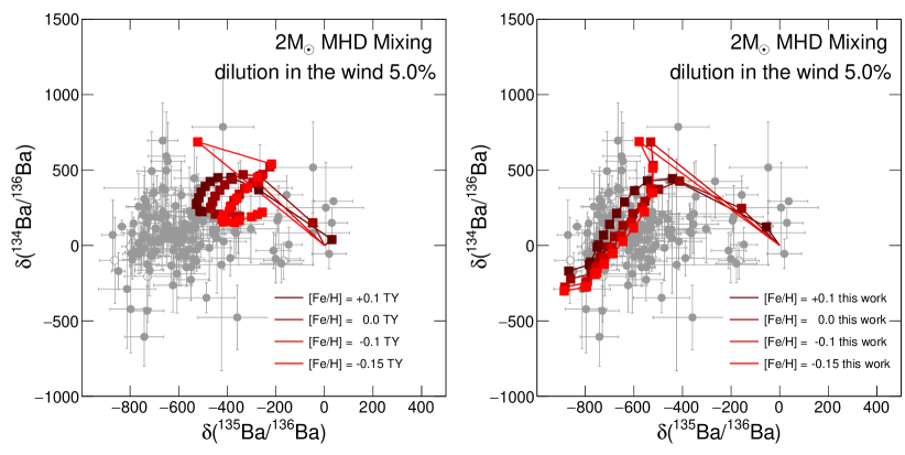
Figure 2: Left panel: isotopic ratios of ¹³⁴Ba and ¹³⁵Ba with respect to ¹³⁶Ba, displayed as part-per-mil deviations from the solar ratios (indicated by the symbol $\delta$) computed in recent AGB models (Palmerini et al., 2021), with cross sections from the KADoNiS v1.0 database and decay rates from TY. Right panel: the results of the same models, where only the decay rates for ¹³⁴Cs and ¹³⁵Cs are changed, using those of the present work. We remind that computations in Palmerini et al. (2021) are from 2 M_⊙ stars, where magneto-hydrodynamic processes induce the penetration of protons into He-rich layers, producing ¹³C then releasing neutrons through ${}^{13}\mathrm{C}(\alpha,n)^{16}\mathrm{O}$. Abundances are computed in stellar winds, where we assume that magnetic blobs further add 5% of s-process rich material in flare-like episodes. The symbol [Fe/H] indicates $\log(X_{\mathrm{F}e}/X_{\mathrm{H}})_{star}-\log(X_{\mathrm{F}e}/X_{\mathrm{H}})_{sun}$. Curves with different colors refer to stellar models of different metallicity.

A further implication of our half-life revision concerns the solar distribution of $s$-elements. In this regard, very recently rather extensive analyses of neutron captures in AGB stars pointed out how a reappraisal of the rates here presented for $\beta^{-}$ decays, with a more accurate treatment of their dependence on temperature and density, was crucial for any improvement in our understanding of the isotopic admixture of Ba in the Sun (Busso et al., 2021). In particular, it was shown that (see Fig. 4 in Busso et al. 2021) an average model could be identified, suitable to mimic (if properly normalized) the outcomes of a simulation from a chemical evolution model of the Galaxy at least for the $s$-process contribution to heavy nuclei. In those estimates, ¹³⁴Ba and ¹³⁶Ba should be both at the level of one, as they do not receive contributions from other processes. In Fig. 3 we show the results of the calculations carried out using the same physical models and nuclear parameters as in Busso et al. (2021), only updating the two rates discussed here. The percentage of s-process contributions to the isotope production is plotted in $\log$ scale (thus for $\log(s)=0$ the contribution is s-only). With blue dots we show the original results for $s$-only nuclei sited close to the magic neutron number $N=82$. In red we report the new values found for ¹³⁴Ba and ¹³⁶Ba using our new rates (all the rest remaining untouched). We stress that the improvement over the previous expectations is striking. We notice that similar improvements are also expected for Galactic Chemical Evolution models computed with full stellar evolutionary yields (Prantzos et al., 2020), which were showed to have severe problems with ¹³⁴Ba and ¹³⁶Ba.

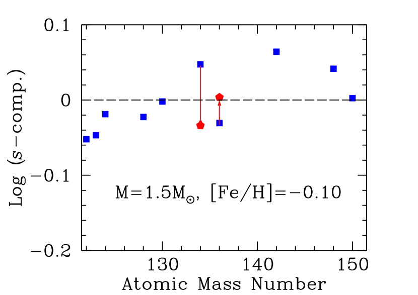
Figure 3: Percentage of $s$-process contributions (blue dots) as computed by Busso et al. (2021), for $s$-only nuclei near the magic neutron number $N=82$. In a perfect model, without nuclear or stellar uncertainties, all points should be aligned at zero. Red points (marked by arrows) show the results for ¹³⁴Ba and ¹³⁶Ba in a revised calculation where, all the rest remaining the same, we adopted the $\beta^{-}$-decay rates for ¹³⁴Cs and ¹³⁵Cs computed in the present work. We note that two more nuclei look as outliers in the figure. They are ¹⁴²Nd and ¹⁴⁸Sm, whose abundances are critically linked to the decay rates of ¹⁴²Pr, ¹⁴⁷Nd and ¹⁴⁸Pm, for which a revision like the present one would be needed.

In conclusion, we find that the $\beta$-decay rates of the ¹³⁴Cs and ¹³⁵Cs isotopes remain lower (even by large factors for ¹³⁴Cs) than the widely used TY estimates, thus pointing to longer half-lives at temperatures $T>10^{8}$ K, which characterize the regions of the AGB stars where the s-process nucleosynthesis occurs. This condition applies to both Cs isotopes even after considering that the rates are dramatically increased at high temperature by two concurrent factors: the inclusion of both the nuclear and the electronic ESs of parent and daughter nuclei, up to complete ionization. Most notably: i) the 60 keV nuclear ES of ¹³⁴Cs, while scarcely populated, is the fastest to $\beta$-decay, with a rate $\simeq$80 times higher than the GS-to-GS one; ii) the rate increases with respect to GS decay only, close to a factor of $\simeq$3 at 20 keV, $\simeq$6 at 30 keV, $\simeq$8 at 40 keV. For ¹³⁵Cs similar effects, concurrent in lowering the half-life, were found, and our results are within the standard deviation of the general systematics.

The use of the new rates to s-process computations in AGB stars remarkably reconciles models and observations for both the Sun and the presolar SiC grain isotopic composition by leading to an overall decrease in the ¹³⁴Ba/¹³⁶Ba and ¹³⁵Ba/¹³⁶Ba abundance ratios predictions, and provides realistic inputs and comparisons to the now forthcoming experiments (Mascali et al., 2017, 2022).

Appendix A Theoretical and computational model

Here we recap few mathematical and computational details of our method for calculating $\beta$-decay in astrophysical scenarios. In the traditional approach, $\beta$-decay spectra of allowed and forbidden transitions are calculated by using an analytical expression of the rate (Hayen et al., 2018) where several factors appear, which account for the nuclear and phase-space structure, and for the atomic exchange. Instead, our approach is based on the calculation of the total Hamiltonian of the system:

$$\mathcal{H}=\mathcal{H}_{\mathrm{nucl}}+\mathcal{H}_{\mathrm{e-e}}+\mathcal{H}_{\mathrm{weak}},$$ (A1)

where $\mathcal{H}_{\mathrm{nucl}}$ contains the interactions between nucleons in the initial and final nuclear states, $\mathcal{H}_{\mathrm{e-e}}$ is the electron-electron Coulomb correlation, taking into account that the transition occurs inside a partially ionized atom, and finally $\mathcal{H}_{\mathrm{weak}}$ is the zero-order QED weak interaction, which fulfills the Lorentz-invariance:

$$\mathcal{H}_{\text{weak}}=\frac{G_{F}}{\sqrt{2}}H_{\mu}L^{\mu}+\mathrm{h.c.},$$ (A2)

where $G_{F}=1.16637\times 10^{-5}GeV^{-2}$, $L^{\mu}$ is the lepton current:

$$L^{\mu}=\bar{u}_{e}\gamma^{\mu}(1-\gamma^{5})v_{\nu},$$ (A3)

and $H_{\mu}$ is the hadronic current:

$$H_{\mu}=\bar{u}_{p}\gamma_{\mu}\left(1-x\gamma^{5}\right)v_{n}.$$ (A4)

In Eqs. (A3,A4) $\gamma^{\mu},\mu=0,...,4$ are the Dirac matrices, $x$ is the ratio between the axial vector coupling constant $c_{A}$ and the vector coupling constant $c_{V}$, $\frac{c_{A}}{c_{V}}\sim 1.2756$, and $u_{e},v_{\nu},v_{n},u_{p}$ are the $\beta$-electron, neutrino, neutron and proton annihilation operators, respectively.

In particular, we are interested in reckoning the probability per unit time that the atomic system decays from a statistical mixture of initial states $\hat{\rho}_{i}=p_{i}|i><i|$ to a mixture of final states $P_{f}=\sum_{f}|f><f|$, that is:

$$N_{i\rightarrow f}=2\pi\mathrm{Tr}(\hat{\rho}_{i}\mathcal{H}_{\text{weak}}P_{f}\mathcal{H}_{\text{weak}})\delta(E_{i}-E_{f})+h.c.$$ (A5)

In the typical approximation to the general theory of $\beta$-decay, where the recoil energy of the final nucleus is small with respect to the nucleon rest mass, the initial and final states can be written as:

$$|i\rangle=|h_{i}\rangle\otimes|e_{i}\rangle$$ (A6)

$$|f\rangle=|h_{f}\rangle\otimes|e_{f}\rangle\otimes|\bar{\nu}_{f}\rangle,$$ (A7)

where $|h_{(i,f)}\rangle$ are initial and final multi-nucleon states characterized by the quantum numbers $|J_{(i,f)},M_{(i,f)},T_{(i,f)}\rangle_{\mathrm{nucl}}$, where $J_{(i,f)},M_{(i,f)}$ denote the total angular momentum and its projection along some fixed axis of the initial and final states, respectively, and $T_{(i,f)}$ is the isospin; $|e_{i}\rangle=|j_{i},m_{i};\left[n_{1}^{b}\cdots n_{k}^{b}\right]_{(i)}\rangle_{\mathrm{e-e}}$ is the initial many-electron state, where $\left[n_{1}^{b}\cdots n_{k}^{b}\right]_{(i,f)}$ represent the bound orbitals; finally, $|\bar{\nu}_{f}\rangle$ is the final anti-neutrino state (typically represented by a free plane wave).

We point out that the initial and final multi-nucleon states and the initial multi-electron states are characterized by a discrete spectrum, while the final multi-electron state, which describes the $\beta$ emission, is a continuum state that can be written as a linear combination of external products $|e_{f}>=\sum_{j}I_{j,f}\wedge|\eta_{j,f}>$, where $|\eta_{j,f}>$ describes the $\beta$-electron continuum wavefunction and $I_{j,f}$ represents the final bound state.

Within this framework, the evaluation of the transition operator can be factorized into the product of lepton and hadronic currents (Morresi et al., 2018). This is ultimately due to the large rest mass of the $W$ vector boson that mediates the weak interaction. Furthermore, we can safely assume that electrons and neutrinos are not coupled and thus the lepton current (A3) can be further factorized in the independent product of the neutrino and electron quantum field operators (or, dealing with expectation values, wavefunctions). In this work, we also make the assumption that the hadronic current can be factorized in the product of neutron and proton field operators. The hadronic current separability is basically equivalent to require that only one nucleon within the parent nucleus participates into the decay dynamics. The decaying nucleon is thus an independent particle, uncorrelated to the “core” of the remaining nucleons. Such a core, which couples only geometrically to the decaying nucleon so as to recover the total angular momentum of the parent reactant and of the final daughter nucleus, is approximated by a linear combination of angular momentum wavefunctions. Our approximation assumes the validity of the nuclear shell model. However, this does not represent an intrinsic limit of our method, as the hadronic current for systems where many-body effects are expected to play a paramount role can be assessed separately, via more accurate first-principle approaches (Hjorth-Jensen et al., 2017). The hadronic current (A4) is derived by an explicit numerical solution of the Dirac equation (DE) in a central potential. In our solution, protons and neutrons interact via a semi-empirical scalar and vector relativistic Wood-Saxon (WS) spherical symmetric potential, which describes the nucleon-nucleon interaction (Schwierz et al., 2007), whereby the DE is mono-dimensional in the radial variable. To solve the equation, a grid with a few thousands points is used (Morresi et al., 2018).

Table 3: $n_{e}/n_{p}$ and $(n_{e}-n_{p})/n_{p}$ ratios of proton densities $n_{p}=10^{26}$ and $n_{p}=10^{27}$ (cm^-3) and of the resulting electron densities $n_{e}$ as a function of temperatures $T$ (keV).

	$n_{p}=10^{26}$		$n_{p}=10^{27}$
$T$	$n_{e}/n_{p}$	$(n_{e}-n_{p})/n_{p}$	$n_{e}/n_{p}$	$(n_{e}-n_{p})/n_{p}$
10	1.0	0.0	1.0	0.0
20	1.0	2.121e-18	1.0	2.234e-21
30	1.0	2.381e-10	1.0	2.57342e-13
40	1.0	2.5098e-06	1.0	2.74123e-09
50	1.0009	0.00087	1.0	9.5167e-07
60	1.0460	0.0460	1.00005	5.3074e-05
70	1.5858	0.5858	1.001025	0.001025
80	3.5663	2.5663	1.010026	0.010026
90	8.0831	7.0831	1.0599	0.05987
100	16.61334	15.61334	1.2334	0.2333676

Also the electron wavefunctions are found by solving self-consistently the Dirac-Hartree-Fock (DHF) equation in a central potential. Electrons interact via a mean-field, where the non-local exchange (Fock term) is replaced by the local density approximation (LDA) to the electron gas ($V_{ex}\propto\rho(r)^{1/3}$) (Slater, 1951; Salvat et al., 1987). The numerical solution of the DHF equation was found by using a modified Runge-Kutta method (Morresi et al., 2018). The non-orthogonality between the bound initial $n_{i}^{b}$ and final $n_{f}^{b}$ orbitals, which are obtained by solving the DHF equations for the parent and daughter nuclei carrying a different atomic number, is taken into account. The continuum $\beta$-electron wavefunction $\psi_{f,e}^{c}(\bf{r})$ is then expressed in the field produced by both the nucleus and the surrounding electrons as a Slater determinant, to take into account the atomic exchange. The $\beta$-electron continuum wavefunction within this framework thus reflects the fact that the emitted lepton may decay into a bound state of the daughter nucleus with ejection of a secondary bound electron and that final state excitations, such as shake-up and shake-off (Morresi et al., 2018), can be present. Atomic exchange effects open up multiple decay channels that typically increase the $\beta$-decay rate particularly at low energies (Harston & Pyper, 1992), where the overlap between the continuum and discrete wave functions maximizes.

Electrons populate the energy levels according to a Fermi-Dirac (FD) distribution $n_{e^{-}}^{i}=\frac{1}{1+e^{(\epsilon_{i}-\mu_{e^{-}})/(K_{\mathrm{B}}T)}}=F(T,\mu_{e^{-}})$, where $K_{\text{B}}$ is the Boltzmann constant and $T$ is the temperature. The eigenvalues $\epsilon_{i}$ are obtained by a self-consistent solution of the DHF equation for the leptons, and the chemical potential is assessed by assuming that the electrons behave as an ideal Fermi gas in a box with a relativistic energy-momentum dispersion $E^{2}=c^{2}p^{2}+m_{e}^{2}c^{4}$ as $n_{e^{-}}=\int_{0}^{\infty}dp~{}p^{2}/\pi^{2}\times(F((c\times\sqrt{(}p^{2}+m_{e}^{2}c^{2})-\mu_{e})/K_{\mathrm{B}}T)-F((c\times\sqrt{(}p^{2}+m_{e}^{2}c^{2})+\mu_{e})/K_{\mathrm{B}}T))$. We notice that the electron orbitals of Cs and Ba have not been re-optimized at each temperature. At very high temperature, however, we included positron formation in our model. The plasma at a given temperature is assumed overall neutral, that is $n_{p}=n_{e^{-}}-n_{e^{+}}$, where $n_{p},n_{e^{-}},n_{e^{+}}$ are the proton, electron, and positron density, respectively. Note that $n_{p}\approx n_{e^{-}}$ at high densities, while they can differ sensibly a low densities. Protons are treated as nonrelativistic particles and their density has been varied in the range $n_{p}=10^{24}-10^{27}$ to model different astrophysical scenarios. In Table 3 we report the proton vs. relevant electron densities at different temperatures.

Appendix B Half-life tables

Here we report the half-lives of both ¹³⁴Cs and ¹³⁵Cs on a finer mesh.

Table 4: ¹³⁴Cs half-lives (years) obtained by our model for several densities (cm^-3) and temperatures $T$ (keV).

$T$	$n_{p}$
	$6\text{\times}{10}^{24}$	$6\text{\times}{10}^{25}$	$6\text{\times}{10}^{26}$	$6\text{\times}{10}^{27}$	$6\text{\times}{10}^{28}$	$6\text{\times}{10}^{29}$
0.86	2.04149	2.05406	2.07755	2.15924	2.55484	5.56986
1.085	2.03336	2.05026	2.07621	2.15899	2.5548	5.56984
1.37	2.01435	2.04481	2.07446	2.15896	2.55518	5.57079
1.719	1.9947	2.03652	2.07328	2.16047	2.55763	5.57629
2.16	1.98896	2.02753	2.07546	2.16711	2.56659	5.59606
2.725	2.00225	2.02915	2.08667	2.18582	2.59062	5.64877
3.43	2.03635	2.05478	2.11409	2.2243	2.63937	5.75549
4.319	2.07298	2.10883	2.16471	2.2886	2.72088	5.93362
5.44	2.00961	2.17161	2.23866	2.37687	2.83378	6.1752
6.845	1.86683	2.1586	2.30543	2.46085	2.94249	6.35983
8.62	1.78273	1.97719	2.24599	2.43095	2.90337	6.01333
10.85	1.58026	1.64867	1.87921	2.08555	2.4593	4.55354
13.66	1.17738	1.19422	1.29305	1.45373	1.67893	2.70035
17.19	0.765335	0.769108	0.798542	0.886004	1.00964	1.47377
21.65	0.48386	0.484805	0.493239	0.533676	0.606594	0.84334
27.25	0.321219	0.321509	0.324257	0.342418	0.389374	0.530591
34.31	0.228839	0.228947	0.229995	0.238386	0.269924	0.365959
43.19	0.174786	0.174833	0.175296	0.179417	0.200815	0.27283
54.37	0.141613	0.141634	0.141865	0.144038	0.158478	0.215895
68.453	0.120307	0.120315	0.120432	0.121659	0.131326	0.178361
86.17	0.106109	0.106113	0.106165	0.106871	0.113322	0.151812

Table 5: ¹³⁵Cs half-lives (years) obtained by our model for several densities (cm^-3) and temperatures $T$ (keV).

$T$	$n_{p}$
	$6\text{\times}{10}^{24}$	$6\text{\times}{10}^{25}$	$6\text{\times}{10}^{26}$	$6\text{\times}{10}^{27}$	$6\text{\times}{10}^{28}$	$6\text{\times}{10}^{29}$
0.86	2.24735e+06	2.28314e+06	2.35169e+06	2.5949e+06	4.05442e+06	1.38295e+08
1.085	2.22363e+06	2.27205e+06	2.34741e+06	2.59384e+06	4.05376e+06	1.38122e+08
1.37	2.16957e+06	2.25504e+06	2.3407e+06	2.59214e+06	4.05272e+06	1.37847e+08
1.719	2.11206e+06	2.22521e+06	2.33048e+06	2.58945e+06	4.05111e+06	1.37424e+0
2.16	2.07881e+06	2.17983e+06	2.31431e+06	2.58509e+06	4.04856e+06	1.36759e+08
2.725	2.06411e+06	2.1325e+06	2.28881e+06	2.57781e+06	4.04444e+06	1.35701e+08
3.43	2.0522e+06	2.09846e+06	2.25322e+06	2.56603e+06	4.03796e+06	1.34072e+08
4.319	1.97606e+06	2.07086e+06	2.21036e+06	2.54721e+06	4.02766e+06	1.3157e+08
5.44	1.62748e+06	1.9987e+06	2.16292e+06	2.51833e+06	4.01129e+06	1.27794e+08
6.845	1.24302e+06	1.75501e+06	2.09403e+06	2.47574e+06	3.9854e+06	1.22285e+08
8.62	1.10909e+06	1.39724e+06	1.94529e+06	2.41137e+06	3.94404e+06	1.14477e+08
10.85	1.07248e+06	1.18395e+06	1.67416e+06	2.29764e+06	3.85507e+06	9.81098e+07
13.66	806399	834310	1.02279e+06	1.44121e+06	2.24393e+06	1.27362e+07
17.19	72041.5	72659.3	77637.2	94275.4	123468	340712
21.65	3851.17	3865.52	3995.78	4683.27	6254.44	16801.2
27.25	358.829	359.506	365.995	412.098	563.022	1513.15
34.31	53.6033	53.6588	54.2028	58.7768	80.1084	214.686
43.19	11.6125	11.6195	11.6889	12.3265	16.2948	42.9303
54.37	3.34727	3.34841	3.36067	3.47855	4.37922	11.0515
68.453	1.20894	1.20911	1.2117	1.23923	1.47913	3.46087
86.17	0.527193	0.527237	0.527765	0.535284	0.609228	1.28288

Table 6: ¹³⁴Cs and ¹³⁵Cs half-lives (years) obtained by our model at Earth conditions without (wcf) the correction factor in comparison to experimental data (Obs.). The correction factors to reproduce the measured half-lives are 4.4 and $\approx$90 for ¹³⁴Cs and ¹³⁵Cs, respectively.

	Obs.	wcf
134Cs	2.0652	8.80
135Cs	2.3e+06	0.025e+06

References

- Ahumada & et al. (2020) Ahumada, R., & et al. 2020, ApJS, 249, 3, doi: 10.3847/1538-4365/ab929e
- Busso et al. (2021) Busso, M., Vescovi, D., Palmerini, S., Cristallo, S., & Antonuccio-Delogu, V. 2021, ApJ, 908, 55, doi: 10.3847/1538-4357/abca8e
- Dillmann et al. (2014) Dillmann, I., Szücs, T., Plag, R., et al. 2014, Nuclear Data Sheets, 120, 171, doi: 10.1016/j.nds.2014.07.038
- Harston & Pyper (1992) Harston, M. R., & Pyper, N. C. 1992, Phys. Rev. A, 45, 6282, doi: 10.1103/PhysRevA.45.6282
- Hayen et al. (2018) Hayen, L., Severijns, N., Bodek, K., Rozpedzik, D., & Mougeot, X. 2018, Rev. Mod. Phys., 90, 015008, doi: 10.1103/RevModPhys.90.015008
- Hjorth-Jensen et al. (2017) Hjorth-Jensen, M., Lombardo, M. P., & van Kolck, U., eds. 2017, An Advanced Course in Computational Nuclear Physics, Vol. 936 (Springer), doi: 10.1007/978-3-319-53336-0
- Langanke et al. (2021) Langanke, K., Martínez-Pinedo, G., & Zegers, R. G. T. 2021, Reports on Progress in Physics, 84, 066301, doi: 10.1088/1361-6633/abf207
- Li et al. (2021) Li, K.-A., Qi, C., Lugaro, M., et al. 2021, The Astrophysical Journal Letters, 919, L19, doi: 10.3847/2041-8213/ac260f
- Mascali et al. (2017) Mascali, D., Musumarra, A., Leone, F., et al. 2017, The European Physical Journal A, 53, 145, doi: 10.1140/epja/i2017-12335-1
- Mascali et al. (2022) Mascali, D., Santonocito, D., Amaducci, S., et al. 2022, Universe, 8, 80, doi: 10.3390/universe8020080
- Morresi et al. (2018) Morresi, T., Taioli, S., & Simonucci, S. 2018, Advanced Theory and Simulations, 1, 1870030
- Nomoto et al. (2013) Nomoto, K., Kobayashi, C., & Tominaga, N. 2013, Annual Review of Astronomy and Astrophysics, 51, 457, doi: 10.1146/annurev-astro-082812-140956
- Palmerini et al. (2016) Palmerini, S., Busso, M., Simonucci, S., & Taioli, S. 2016, Journal of Physics: Conference Series, 665, 012014
- Palmerini et al. (2021) Palmerini, S., Busso, M., Vescovi, D., et al. 2021, The Astrophysical Journal, 921, 7, doi: 10.3847/1538-4357/ac1786
- Prantzos et al. (2020) Prantzos, N., Abia, C., Cristallo, S., Limongi, M., & Chieffi, A. 2020, Monthly Notices of the Royal Astronomical Society, 491, 1832
- Salvat et al. (1987) Salvat, F., Martìnez, J. D., Mayol, R., & Parellada, J. 1987, Phys. Rev. A, 36, 467, doi: 10.1103/PhysRevA.36.467
- Schwierz et al. (2007) Schwierz, N., Wiedenhover, I., & Volya, A. 2007, arXiv:0709.3525 [nucl-th]
- Simonucci et al. (2013) Simonucci, S., Taioli, S., Palmerini, S., & Busso, M. 2013, The Astrophysical Journal, 764, 118
- Singh et al. (2008) Singh, B., Rodionov, A. A., & Khazov, Y. L. 2008, Nuclear Data Sheets, 109, 517, doi: https://doi.org/10.1016/j.nds.2008.02.001
- Slater (1951) Slater, J. C. 1951, Phys. Rev., 81, 385, doi: 10.1103/PhysRev.81.385
- Sonzogni (2004) Sonzogni, A. 2004, Nuclear Data Sheets, 103, 1, doi: https://doi.org/10.1016/j.nds.2004.11.001
- Takahashi & Yokoi (1983) Takahashi, K., & Yokoi, K. 1983, Nuclear Physics A, 404, 578, doi: https://doi.org/10.1016/0375-9474(83)90277-4
- Takahashi & Yokoi (1987) —. 1987, Atomic Data and Nuclear Data Tables, 36, 375, doi: https://doi.org/10.1016/0092-640X(87)90010-6
- Vescovi et al. (2019) Vescovi, D., Piersanti, L., Cristallo, S., et al. 2019, Astronomy & Astrophysics, 623, 7