Equivariant Neural Network for Factor Graphs

Abstract

Several indices used in a factor graph data structure can be permuted without changing the underlying probability distribution. An algorithm that performs inference on a factor graph should ideally be equivariant or invariant to permutations of global indices of nodes, variable orderings within a factor, and variable assignment orderings. However, existing neural network-based inference procedures fail to take advantage of this inductive bias. In this paper, we precisely characterize these isomorphic properties of factor graphs and propose two inference models: Factor-Equivariant Neural Belief Propagation (FE-NBP) and Factor-Equivariant Graph Neural Networks (FE-GNN). FE-NBP is a neural network that generalizes BP and respects each of the above properties of factor graphs while FE-GNN is an expressive GNN model that relaxes an isomorphic property in favor of greater expressivity. Empirically, we demonstrate on both real-world and synthetic datasets, for both marginal inference and MAP inference, that FE-NBP and FE-GNN together cover a range of sample complexity regimes: FE-NBP achieves state-of-the-art performance on small datasets while FE-GNN achieves state-of-the-art performance on large datasets.

1 Introduction

Probabilistic graphical models (PGM) provide a statistical framework for modeling dependencies between random variables. Performing inference on PGMs is a fundamental task with many real-world applications including statistics, physics, and machine learning [3, 20, 29, 1, 24]. Factor graphs are a general way of representing PGMs. As a data structure, a factor graph can be viewed as a bipartite graph of variables and factors; each factor node indicates the presence of dependencies among the variables it is connected to. Many inference algorithms have been developed to leverage the conditional independence structure imposed by a factor graph representation. Among these, Belief Propagation (BP) [13] has demonstrated empirical success in a variety of applications such as error correction decoding algorithms [18] and combinatorial optimization [2].

Despite their empirical success, traditional inference algorithms like BP are handcrafted and perform the same computational procedures for any input PGM, limiting their accuracy. Thus, researchers have started to develop trainable neural network-based inference models [15, 27, 33, 34], aiming to enable inference algorithms to adapt by learning from data. However, prior works have treated factor graphs simply as bipartite graphs, overlooking the more complex isomorphisms associated with factor graphs. Recently, [15] presents a description of factor graph isomorphism yet it is incomplete and lacks empirical evidence. In this work, we present a complete description of factor graph isomorphism, with empirical evidence of improved inductive bias.

We propose two neural network-based inference models that leverage these factor graph isomorphism properties to improve their inductive bias: Factor-Equivariant Neural Belief Propagation and (FE-NBP) and Factor-Equivariant Graph Neural Networks (FE-GNN). FE-NBP is a neural network that adopts the message passing procedure of standard BP but incorporates a neural network module that learns adaptive damping ratios while updating the messages. FE-NBP fully respects factor graph isomorphism. FE-GNN is an end-to-end inference model parameterized by a graph neural network (GNN) tailored for factor graphs. Compared with other existing GNN-based inference models, FE-GNN has a better inductive bias; compared with BP or FE-NBP, its discriminative power can be leveraged when a larger amount of training instances is available.

Using one of the most common experimental settings for evaluating probabilistic inference algorithms – marginal inference on Ising models, we show that FE-NBP achieves state-of-the-art performance on small datasets while FE-GNN achieves state-of-the-art performance on large datasets. We further conduct experiments on factor graphs where at least one factor potential is not a symmetric tensor and show dramatic improvement of FE-GNN over other existing GNN-based inference models. This supports our claim that respecting factor graph isomorphism improves the inductive bias of neural architectures that perform inference on factor graphs. We also conduct experiments on real-world UAI-challenge datasets and demonstrate that FE-NBP outperforms existing inference models on MAP inference.

We summarize our contributions as follows:

• We identify a previously overlooked isomorphism between factor graphs and empirically demonstrate the effectiveness of incorporating it as an inductive bias.

• We propose Factor-Equivariant Neural Belief Propagation (FE-NBP), a neural architecture that performs inference on factor graphs. FE-NBP generalizes belief propagation by learning adaptive damping ratios while fully respecting factor graph isomorphism. Experiments conducted on both Ising models and UAI-challenge datasets manifest the effectiveness of FE-NBP.

• We propose Factor-Equivariant Graph Neural Networks (FE-GNN), an end-to-end GNN-based inference model that respects more conditions of factor graph isomorphisms than existing GNNs. In our experiments, we demonstrate that FE-GNN is superior to other existing GNN-based inference models.

• Empirically, we show that FE-NBP and FE-GNN together cover a wide range of sample complexity regimes and discuss the trade-offs between different classes of models.

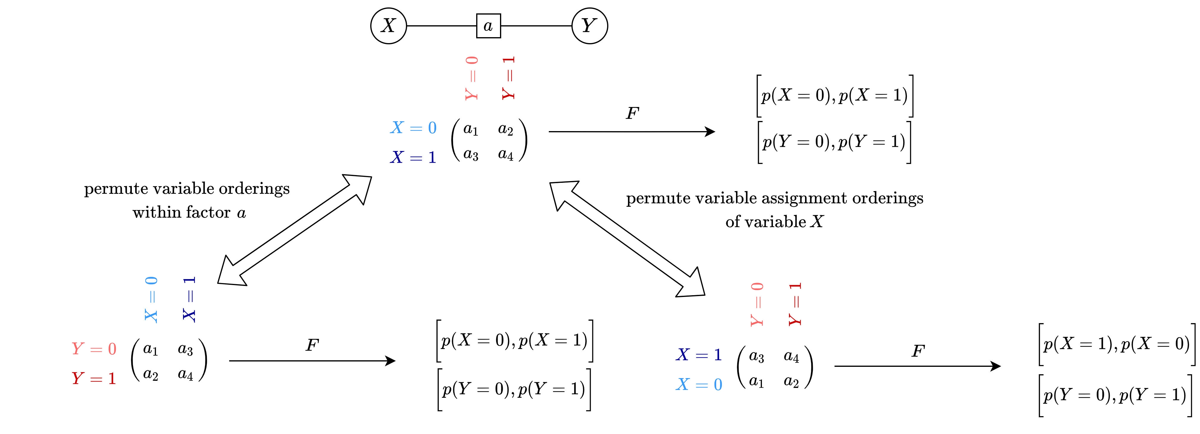
Figure 1: Consider a factor graph with one factor and two variables $X$ and $Y$. Both variables are binary and thus the factor potential $a$ is a 2 by 2 tensor. Note all three factor graphs in the figure are isomorphic. That is, all three represent the same probability distribution and are related by bijective mappings. $F$ is a function or algorithm that takes a factor graph as input and outputs an ordered list of vectors where each vector represents marginal estimates for a variable. If we permute variable orderings ($X,Y$ to $Y,X$) within factor $a$ and $F$ gives invariant outputs, $F$ respects Local Variable Symmetry of factor graph isomorphism. If we permute variable assignments within a variable ($X=0,X=1$ to $X=1,X=0$) and $F$ gives equivariant outputs, $F$ respects Variable Assignment Symmetry of factor graph isomorphism (the dimension of marginal vectors permute accordingly)

.

2 Background

In this section we provide background on factor graphs [14, 32], belief propagation [13], and graph neural networks [10, 28, 12].

Factor Graph

A factor graph is a compact representation of a discrete probability distribution that takes advantage of (conditional) independencies among variables. Let $p$ be a distribution defined over $n$ discrete random variables $\{X_{1},X_{2},\dots,X_{n}\}$. Let $x_{i}$ denote a possible assignment of the $i^{th}$ variable. We use the shorthand $p(\mathbf{x})=p(X_{1}=x_{1},\dots,X_{n}=x_{1})$ for the joint probability mass function, where $\mathbf{x}=\{x_{1},x_{2},\dots,x_{n}\}$ is a realization of all $n$ variables. Without loss of generality, $p(\mathbf{x})$ can be written as following:

$$p(\mathbf{x})=\frac{1}{Z}\prod_{a=1}^{M}f_{a}(\mathbf{x}_{a}),\quad\ \ \ \ \ \ \ Z=\sum_{\mathbf{x}}\Bigg{(}\prod_{a=1}^{M}f_{a}(\mathbf{x}_{a})\Bigg{)}.$$ (1)

The factor graph is defined in terms of a set of factors $\{f_{1},f_{2},\dots,f_{M}\}$, where each factor $f_{a}$ takes a subset of variable’s assignments $\mathbf{x}_{a}\subset\{x_{1},x_{2},\dots,x_{N}\}$ as input and $f_{a}(\mathbf{x}_{a})>0$. $Z$ is the factor graph’s normalization constant (or partition function). As a data structure, a factor graph is a bipartite graph with $N$ variables nodes and $M$ factor nodes. Factor nodes and variables nodes are connected if and only if the variable is in the scope of the factor. For readability, we will use $a$ and $b$ to index factors, $i$ and $j$ to index variables, upper-case $X_{i}$ to indicate variable $i$, and lower-case $x_{l}$ to indicate a variable assignment.

Belief Propagation

Belief propagation (BP) is a method for estimating marginal distribution of variables and the partition function (marginal inference). BP performs iterative message passing among neighboring variable and factor nodes. For numerical stability, belief propagation is generally performed in log-space, and messages are normalized at every iteration.Variable to factor messages (variable $X_{i}$ to factor $f_{a}$), $\bm{m_{i\rightarrow a}^{(k)}}$, and factor to variable messages (factor $f_{a}$ to variable $X_{i}$), $\bm{m_{a\rightarrow i}^{(k)}}$, are computed at every iteration $k$ as

$$m_{i\rightarrow a}^{(k)}(x_{l}) =-z_{i\rightarrow a}+\sum_{c\in\mathcal{N}(i)\setminus a}m_{c\rightarrow i}^{(k-1)}(x_{l}),$$ (2)

$$\tilde{m}_{a\rightarrow i}^{(k)}(x_{l}) =-z_{a\rightarrow i}+\underset{\mathbf{x}_{a}\setminus X_{i}=x_{l}}{\text{LSE }}\bigg{(}\Psi_{a}(\mathbf{x}_{a})+\sum_{j\in\mathcal{N}(a)\setminus i}m_{j\rightarrow a}^{(k)}(x_{j})\bigg{)}.$$ (3)

We use the shorthand $m_{i\rightarrow a}^{(k)}(x_{l})$ and $m_{a\rightarrow i}^{(k)}(x_{l})$ to denote $m_{i\rightarrow a}^{(k)}(X_{i}=x_{l})$ and $m_{a\rightarrow i}^{(k)}(X_{i}=x_{l})$, respectively. Note that $\bm{m_{i\rightarrow a}^{(k)}}$ and $\bm{m_{a\rightarrow i}^{(k)}}$ are vectors of size $|X_{i}|$ and $m_{i\rightarrow a}^{(k)}(x_{l})$ and $m_{a\rightarrow i}^{(k)}(x_{l})$ are scalars. $\Psi_{a}(\mathbf{x}_{a})=\ln\left(f_{a}\left(\mathbf{x}_{a}\right)\right)$ denotes log factor potentials, $z_{i\rightarrow a}$ and $z_{a\rightarrow i}$ are normalization terms, and $\mathcal{N}(a)$ and $\mathcal{N}(i)$ denote the nodes adjacent to $a$ and $i$ respectively. We use the shorthand $\underset{}{\text{LSE }}$ for the log-sum-exp function. The subscript $\mathbf{x}_{a}\setminus X_{i}=x_{l}$ means that we iterate over all variable realizations of variables connected to factor $a$ except that variable $X_{i}$ is fixed to an assignment of $x_{l}$.

The belief propagation algorithm proceeds by iteratively updating variable to factor messages and factor to variable messages until they converge or a predefined maximum number of iterations is reached. Variable beliefs $b^{(k)}_{i}$ and factor beliefs $b^{(k)}_{a}$ are computed to estimate marginals

$$b^{(k)}_{i}(x_{l})\propto\exp\Big{(}\sum_{a\in\mathcal{N}(i)}m_{a\rightarrow i}^{(k)}(x_{l})\Big{)},\,\,b^{(k)}_{a}(\mathbf{x}_{a})\propto\exp\bigg{(}\Psi_{a}(\mathbf{x}_{a})+\sum_{j\in\mathcal{N}(a)}m_{j\rightarrow a}^{(k)}(x_{j})\bigg{)}$$ (4)

To perform MAP inference with BP, we replace the the log-sum-exp function in Equation 3 with max and decoding variable assignments using variable beliefs $\hat{x}_{i}^{*}=\arg\max_{x_{i}}b_{i}(x_{i})$.

Graph Neural Networks

Graph Neural Networks (GNNs) take an input graph $G=(V,E)$ with or without node features and edge features and learn representation vectors of all nodes. Modern GNNs follow a neighborhood aggregation strategy [31, 8], where we iteratively update the representation of a node by aggregating representations of its neighbors. After $k$ iterations of aggregation, a node’s representation captures the structural information within its $k$-hop network neighborhood. Formally, the $k$-th layer of a GNN with edge features is

$$h_{v}^{(k)}=\phi\left(h_{v}^{(k-1)},f\left(\left\{\left(h_{u}^{(k-1)},e_{uv}\right):u\in\mathcal{N}(v)\right\}\right)\right)$$ (5)

where $h_{v}^{(k)}$ is the feature vector of node $v$ at the $k$-th iteration/layer, $\mathcal{N}(v)$ is a set of nodes adjacent to $v$, and $e_{uv}$ is the feature vector of edge $(u,v)$. The choice of $\phi$ and $f$ can be crucial in GNNs [30].

3 Methodology

Ideally, an inference algorithm should produce equivalent (or equivariant) outputs for two isomorphic factor graphs. This is a property that BP satisfies, but is overlooked by existing works that perform probabilistic inference using neural networks. We aim to address this problem in this paper.

3.1 Factor Graph Isomorphism

In this section we characterize three conditions of factor graph isomorphism, an equivalence relation between factor graphs.

Definition 1.

1. Global Symmetry: permuting the global indices of variables or factors in a factor graph results in an isomorphic factor graph. A function or algorithm $F$ respects Global Symmetry if the output of $F$ is either equivariant or invariant to the permutation of global node ordering.

2. Local Variable Symmetry: permuting the local indices of variables within factors results in an isomorphic factor graph. A function or algorithm $F$ respects Local Variable Symmetry if the output of $F$ is either equivariant or invariant to the permutation of variable orderings within factors.

3. Variable Assignment Symmetry: permuting the variable assignments within variables will result in an isomorphic factor graph. A function or algorithm $F$ respects Variable Assignment Symmetry if the output of $F$ is either equivariant or invariant to the permutation of the orderings of variable assignments within variables.

Find the formal definition of factor graph isomorphism in Appendix A. This concept is further illustrated in Figure 1. Note that whether an algorithm should be either equivariant or invariant to each of the above permutations depend on the output of the inference algorithm. Prior work [15] identified Global Symmetry and Local Variable Symmetry but failed to identify Variable Assignment Symmetry. As we show in our experiments, respecting Variable Assignment Symmetry results in improved performance.

3.2 Factor-Equivariant Neural Belief Propagation

Factor-Equivariant Neural Belief Propagation (FE-NBP) is an inference model that incorporates a neural network on top of BP’s procedures. In BP, factor-to-variable messages are iteratively updated and our key idea is to learn an adapted damping ratio for those updates:

$$m_{a\rightarrow i}^{(k)}(x_{l})=\tilde{m}_{a\rightarrow i}^{(k)}(x_{l})+\alpha^{(k)}_{a\rightarrow i}(x_{l})\big{(}m^{(k-1)}_{a\rightarrow i}(x_{l})-\tilde{m}^{(k)}_{a\rightarrow i}(x_{l})\big{)}$$ (6)

for $a\in[M],i\in[N],l\in[|X_{i}|]$ and $k$ denotes the number of current iterations. $\tilde{m}^{(k)}_{a\rightarrow i}(x_{l})$ has the same definition as in Equation 3. Note that $m_{a\rightarrow i}^{(k)}$ is a vector of size $|X_{i}|$ and $m_{a\rightarrow i}^{(k)}(x_{l})$, being the shorthand of $m_{a\rightarrow i}^{(k)}(X_{i}=x_{l})$, is a scalar in $m_{a\rightarrow i}^{(k)}$.

The damping ratio $\alpha^{(k)}_{a\rightarrow i}(x_{l})$ is adaptive and calculated using a neural network module as follows:

$$\alpha^{(k)}_{a\rightarrow i}(x_{l})=\phi_{\text{NN}}\left({m}^{(k-1)}_{a\rightarrow i}(x_{l}),\tilde{m}^{(k)}_{a\rightarrow i}(x_{l}),b_{i}^{(k)}(x_{l}),\sum_{\mathbf{x}_{a}\backslash X_{i}=x_{l}}b_{a}^{(k)}(\mathbf{x}_{a}),\max_{\mathbf{x}_{a}\backslash X_{i}=x_{l}}b_{a}^{(k)}(\mathbf{x}_{a})\right),$$ (7)

where $b_{i}^{(k)}$ and $b_{a}^{(k)}$ denote variable beliefs and factor beliefs, respectively, following Equation 4. The term $\sum_{\mathbf{x}_{a}\backslash X_{i}=x_{l}}b_{a}^{(k)}(\mathbf{x}_{a})$ denotes factor beliefs summed over all variable realizations of $a$ except that $X_{i}$ it set to an assignment of $x_{l}$. $\max_{\mathbf{x}_{a}\backslash X_{i}=x_{l}}b_{a}^{(k)}(\mathbf{x}_{a})$) denotes maximum factor belief achievable when fixing $X_{i}$ to $x_{l}$ in $\mathbf{x}_{a}$. $\phi_{\text{NN}}$ is a neural network function whose parameters are shared for all updates of the factor-to-variable messages. Output of $\phi_{\text{NN}}$ is a scalar. These five input features are designed based on the intuitions of classical improvements of BP, such as incorporating the information of the residual of messages [7] (i.e. $|{m}^{(k-1)}_{a\rightarrow i}(x_{l})-\tilde{m}^{(k)}_{a\rightarrow i}(x_{l})|$) or inducing more calibrated beliefs [13] (i.e. $|b_{i}^{(k)}(x_{l})-\sum_{\mathbf{x}_{a}\backslash X_{i}=x_{l}}b_{a}^{(k)}(\mathbf{x}_{a})|$ and $|b_{i}^{(k)}(x_{l})-\max_{\mathbf{x}_{a}\backslash X_{i}=x_{l}}b_{a}^{(k)}(\mathbf{x}_{a})|$) to facilitate faster, more often convergence and better performances.

Proposition 1.

For any parameterization of $\phi_{\text{NN}}$, FE-NBP respects Global Symmetry, Local Variable Symmetry, and Variable Assignment Symmetry of factor graph isomorphism in Definiton 1.

We can easily verify that Proposition 1 hold since messages are updated individually similar to BP. Due to the space limit, we leave more detailed proofs and explanations in Appendix B.

In BPNN [15], they also propose to adjust factor-to-variable messages in BP by a neural network. However, FE-NBP offers major advantages over their model: (1) BPNNs does not respect Variable Assignment Symmetry as they apply neural networks directly on message vectors and MLPs are not equivariant to permutation of input vectors. The neural network module $\phi_{\text{NN}}$ in FE-NBP adjusts factor-to-variable messages individually for each variable assignments and thus respects Variable Assignment Symmetry; (2) their neural network only takes in messages as input whereas FE-NBP also incorporates information from variable beliefs and factor beliefs to facilitate the process of calibrating BP’s message updates; (3) in their paper, they only conduct experiments on partition function estimation while we conduct experiments with FE-NBP on both marginal inference and MAP inference. For FE-NBP to perform MAP inference, we simply change the log-sum-exp in Equation 3 to log-max-exp and train our model with MAP inference objectives instead of marginal inference objectives. FE-NBP can provide an upper bound and a lower bound for the probability of the output MAP assignment. Find proof in Appendix C.

3.3 Factor-Equivariant Graph Neural Network

Prior works [13, 34] have attempted to use GNN-based models to perform inference. While these GNN-based models respects Global Symmetry, they do not respect further symmetries of fator graphs. In this section, we first provide a perspective of BP by rewriting its formulation and showing that BP can be considered as a non-parameterized GNN. Building on this observation, we propose Factor-Equivariant GNN, a highly expressive GNN architecture that respects Global Symmetry and Local Variable Symmetry.

Rewriting Message Passing of Belief Propagation

In Equation 2 and 3, $m_{i\rightarrow a}^{(k)}(x_{l})$ and $m_{a\rightarrow i}^{(k)}(x_{l})$ are scalars. In this paragraph, we first rewrite the formulation of a standard log-space BP with damping in terms of vectors and tensors:

$$\bm{m_{i\rightarrow a}^{(k)}} =\bm{\tilde{m}_{i\rightarrow a}^{(k)}}+\alpha\big{(}\bm{m_{i\rightarrow a}^{(k-1)}}-\bm{\tilde{m}_{i\rightarrow a}^{(k)}}\big{)},\,\,\bm{\tilde{m}_{i\rightarrow a}^{(k)}}=-z_{i\rightarrow a}+\sum_{c\in\mathcal{N}(i)\setminus a}\bm{m_{c\rightarrow i}^{(k-1)}},$$ (8)

$$\bm{m_{a\rightarrow i}^{(k)}} =\bm{\tilde{m}_{a\rightarrow i}^{(k)}}+\alpha\big{(}\bm{m_{a\rightarrow i}^{(k-1)}}-\bm{\tilde{m}_{a\rightarrow i}^{(k)}}\big{)},\,\,\bm{\tilde{m}_{a\rightarrow i}^{(k)}}=-z_{a\rightarrow i}+\underset{X_{a}\setminus X_{i}}{\text{LSE }}\bigg{(}\bm{\Psi_{a}}+\bigoplus_{j\in\mathcal{N}(a)\setminus i}\bm{m_{j\rightarrow a}^{(k)}}\bigg{)}.$$ (9)

Vectors and tensors are boldfaced but not scalars. The terms $\bm{m_{i\rightarrow a}^{(k)}}$ and $\bm{m_{a\rightarrow i}^{(k)}}$ are vectors over the states of variable $x_{i}$ and thus have length $|X_{i}|$. Log factor potential, $\bm{\Psi_{a}}$, is a multi-dimensional tensor with shape of $\bigg{(}\left|X_{a1}\right|,\left|X_{a2}\right|,\cdots,\left|X_{aK}\right|\bigg{)}$ where $X_{ai}$ denotes the $i$-th variable that associates with factor $a$. We use $X_{a}$ to denote the set of variables that are connected to factor $a$. Operator $\bigoplus$ denotes “tensor sum” (think of outer sum for tensors not just for one-dimensional vectors):

$$\bm{v}=[v_{1},v_{2},\cdots,v_{m}],\bm{w}=[w_{1},w_{2},\cdots,w_{n}],\bm{v}\bigoplus\bm{w}=\begin{bmatrix}v_{1}+w_{1}&v_{1}+w_{2}&\dots&v_{1}+w_{n}\\ v_{2}+w_{1}&v_{2}+w_{2}&\dots&v_{2}+w_{n}\\ \vdots&\vdots&\ddots&\vdots\\ v_{m}+w_{1}&v_{m}+w_{2}&\dots&v_{m}+w_{n}\end{bmatrix}$$

Thus, $\bigoplus_{j\in\mathcal{N}(a)\setminus i}\bm{m_{j\rightarrow a}^{(k)}}$ would have a dimension of
$\bigg{(}\left|X_{a1}\right|,\left|X_{a2}\right|,\cdots,\left|X_{a(i-1)}\right|,\left|X_{a(i+1)}\right|,\cdots,\left|X_{aK}\right|\bigg{)}$. It is added with $\Psi_{a}$ at all corresponding dimensions except at the dimension of $X_{i}$ and then $\underset{X_{a}\setminus X_{i}}{\text{LSE }}$ would then sum over all other variable dimension except at the dimension of variable $X_{i}$, resulting a vector of size $|X_{i}|$.We make the observation that standard BP is just an instance of GNN without trainable parameters where message passing is performed between message vectors. More specifically, Equation 8 and  9 can be viewed as instances of Equation 5 ($\bm{m_{i\rightarrow a}^{(k)}}$ and $\bm{m_{a\rightarrow i}^{(k)}}$ corresponds to node feature vectors $h_{v}^{(k)}$, damping corresponds to function $\phi$, and the aggregation of neighboring messages corresponds to function $f$).

Factor-equivariant Graph Neural Network

We propose Factor-Equivariant GNN, a GNN architecture that satisfies two important properties of BP: no double counting of messages and is equivariant to permutation of variable orderings within factors. FE-GNN avoids double counting of messages by performing message passing between message vectors instead of variables and factors. The key insight that makes FE-GNN equivariant to permutation of variable orderings within factors is that instead of treating factor potentials as input node or edge features, we combine factor potentials with message vectors in a similar fashion to BP by incorporating an operation unconventional for GNNs - tensor sum.

In detail, the model looks like this:

$$\bm{m_{i\rightarrow a}^{(k)}} =\phi_{\text{NN}_{1}}\left(\bm{m_{i\rightarrow a}^{(k-1)}},\sum_{c\in\mathcal{N}(i)\setminus a}\text{MLP}_{1}\bigg{(}\bm{m_{c\rightarrow i}^{(k-1)}}\bigg{)}\right),$$ (10)

$$\bm{m_{a\rightarrow i}}^{(k)} =\phi_{\text{NN}_{2}}\left(\bm{m_{a\rightarrow i}^{(k-1)}},\underset{X_{a}\setminus X_{i}}{\text{LSE }}\bigg{(}\bm{\Psi_{a}}\,\,+\bigoplus_{j\in\mathcal{N}(a)\setminus i}\text{MLP}_{2}\bigg{(}\bm{m_{j\rightarrow a}^{(k)}}\bigg{)}\right)$$ (11)

where $\bm{m_{j\rightarrow a}^{(k)}}$ and $\bm{m_{a\rightarrow i}^{(k)}}$ are node embeddings at layer $k$. $\bm{m_{c\rightarrow i}^{(k-1)}}$ and $\bm{m_{j\rightarrow a}^{(k-1)}}$ are neighboring node embeddings of $\bm{m_{j\rightarrow a}^{(k)}}$ and $\bm{m_{a\rightarrow i}^{(k)}}$ respectively. $\phi_{\text{NN}_{1}}$ and $\phi_{\text{NN}_{2}}$ are neural network modules, which are implemented as GRUs [5] in our experiments. After multiple message passing layers, variable beliefs (or variable marginals) can be estimated by another neural network module such as $b^{(k)}_{i}=\text{MLP}_{3}\Big{(}\sum_{a\in\mathcal{N}(i)}\bm{m_{a\rightarrow i}^{(k)}}\Big{)}$. FE-GNN is trained end-to-end on an objective just like any other GNNs. In our experiments, FE-GNN is trained directly on ground truth marginals of all variables. Additionally, hand-crafted features like those used by FE-NBP can be concatenated with neighboring node embeddings before all neighboring information is aggregated.

Proposition 2.

For any parameterization of $\phi_{\text{NN}_{1}}$ and $\phi_{\text{NN}_{2}}$, FE-GNN respects Global Symmetry and Local Variable Symmetry of factor graph isomorphism in Definiton 1.

FE-GNN respects Local Variable Symmetry of factor graph isomorphism similar to how BP respects Local Variable Symmetry. The term $\underset{X_{a}\setminus X_{i}}{\text{LSE }}\bigg{(}...\bigg{)}$ is not subject to the orderings of variables within factor $a$ since each transformed message vector is summed with factor potentials $\bm{\Psi_{a}}$ at the dimension that corresponds to the particular variable, and $\underset{X_{a}\setminus X_{i}}{\text{LSE }}$ eventually sums out all the dimension except for the dimension of a particular variable $X_{i}$.

4 Experiments

We conduct three experiments to support our claims of contribution. First, we conduct experiments on Ising model datasets of different sample sizes to demonstrate the competence of FE-NBP and FE-GNN on marginal inference. Second, we evaluate FE-GNN on a synthetic dataset of “asymmetric” factor graphs to support our claim that FE-GNN is superior to other GNN-based models as it respects Local Variable Symmetry. Finally, we conduct experiments on real-world UAI-challenge datasets and show that FE-NBP outperforms BPNN [15] by a large margin, supporting our claim that respecting Variable Assignment Symmetry is a beneficial inductive bias to incorporate.

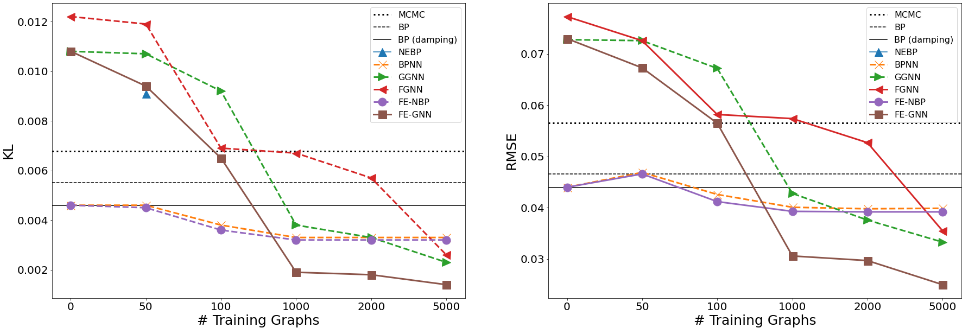
Figure 2: Left: KL divergence between estimated marginals and ground truth for each model trained on Ising model datasets of different sample sizes. Right: RMSE between estimated marginals and ground truth for each model trained on Ising model datasets of different sample sizes.

4.1 Ising Models

The goal of this experiment is to compare FE-NBP and FE-GNN with other existing inference models and to investigate how the amount of training data and the expressiveness of a model affect the performance of each inference model.

Experiment setting

Ising model is a type of Binary Markov Random Field and is usually represented with $(\mathbf{J}$, $\mathbf{b})$ where $\mathbf{b}$ biases individual variables and $\mathbf{J}$ couples pairs of neighbor variables. Following a common experimental settings to evaluate inference algorithms [15, 27, 33], we generate 4x4 grid structured Ising models $(\mathbf{J}$, $\mathbf{b})$ where $\mathbf{x}\in\{+1,-1\}^{|\mathcal{V}|}$, $b_{i}\sim\mathcal{N}(0,0.25^{2})$, $J_{ij}\sim\mathcal{N}(0,1)$ and $|\mathcal{V}|=16$ is the number of variables. Ground truth marginals can be computed exactly using junction tree algorithm [16]. We vary the amount of data the model is trained on and evaluate them on the same testing set of 1000 factor graphs.

We evaluated FE-NBP and FE-GNN against the following baselines: Markov chain Monte Carlo [23], Belief Propagation (BP) [13], BP with damping of 0.5 [22], Neural Enhanced Belief Propagation (NEBP) [26], Belief Propagation Neural Networks (BPNN) [15], Gated Graph Neural Network (GGNN) [17], and Factor Graph Neural Network (FGNN) [34]. For more details of these baselines, refer to the Related Works section. Note that the authors of NEBP did not release their code, thus we take the KL divergence results reported on their paper as we have the same experimental settings. For more model and training details, refer to Appendix D.

Results

As shown in Figure 2, the performance of BP, Damping BP, and MCMC are unchanged as they are not learnable algorithms. Observe that FE-NBP and BPNN, when untrained, both correspond to Damping BP as we initialize all neural network parameters to zero (sigmoid function at 0 equals 0.5). When we have 50 or 100 training instances available, FE-NBP performs the best and all the GNN-based models performs poorly. As we increase the number of training instances to more than 1000, FE-GNN outperforms all baselines and all GNN-based models continue to improve while BPNN and FE-NBP plateaued. The results can be interpreted by the classic bias-variance trade-off: learning algorithms need (inductive) bias tailored to specific learning problems in order to make the target function easier to approximate; learning algorithms also need expressivity so that they can adapt to training data but higher “flexibility” can lead to higher variance. BPNN and FE-NBP are algorithms with high (inductive) bias but are relatively less expressive because they are only learning on top of the backbone of BP, whereas GNN-based models are end-to-end parameterized models with less bias but higher expressiveness. In other words, BPNN and FE-NBP are algorithms in the lower sample complexity regimes while GNN-based models are algorithms in the higher sample complexity regimes.

4.2 Factor-Equivariant GNN on Asymmetric Binary Markov Random Field

To further show that the importance of incorporating Local Variable Symmetry as an inductive bias for neural network-based inference models, we compare FE-GNN with existing GNN-based inference models on a dataset of asymmetric binary markov random field (BMRF) [19]. To clarify, asymmetric means that at least one factor potential is an asymmetric tensor.

Experiment setting

In this experiment, we generate 6000 instances of asymmetric BMRF. 5000 instances are used for training and 1000 for testing. BMRF are generated in a similar fashion to the previous experiment except that now a factor $a$ that couples variable $i$ and $j$ would have a factor potential of $f_{a}=\begin{bmatrix}e^{J_{ij}+J_{ji}}&e^{-2*J_{ij}}\\ e^{-2*J_{ji}}&e^{J_{ij}+J_{ji}}\\ \end{bmatrix}$ where $J_{ij}\sim\mathcal{N}(0,1)$ and $J_{ji}\sim\mathcal{N}(0,1)$. $J_{ij}=J_{ji}=0$ if variable $i$ and $j$ is not coupled by any factor. As for baselines, we compared FE-GNN with Gated Graph Neural Network (GGNN) [33], Factor Graph Neural Network (FGNN) [34], BP [13], and BP with damping (0.5) [22]. We follow the same model and training settings as the previous experiment.

Model	BP	BP (damping)	GGNN	FG-GNN	FE-GNN
KL	0.0286	0.0236	0.3770	0.3780	0.0109
RMSE	0.0818	0.0748	0.3877	0.3877	0.0584

Table 1: KL divergence and RMSE between estimated marginals and ground truth for FE-GNN and other baselines on a dataset of asymmetric binary markov random field.

Results

In Table 1, we present KL divergence and RMSE between estimated marginals and ground truth for each model. FE-GNN outperforms all other models by a significant margin. More importantly, observe how other GNN-based inference models perform poorly. The reason is that existing GNN-based inference models like GGNN or FGNN do not respect Local Variable Symmetry of factor graph isomorphism. More specifically, they treat factor potentials as node/edge features and do not take variable orderings within a factor into consideration. As a result, they fail to learn effectively when factor potentials are asymmetric tensors. This experiment shows that FE-GNN, designed with tensor operations that take variable orderings into consideration, is able to learn on more complex factor graphs given the same amount of training data due to its superior inductive bias.

4.3 Factor-Equivariant Neural BP on the UAI-challenge datasets

In this experiment, we evaluate FE-NBP on MAP inference with the UAI-challenge datasets. We did not evaluate GNN-based models on UAI-challenge datasets as the number of instances in those datasets is very limited and is thus not suitable for evaluating highly expressive models (models with high sample complexity).

Experiment setting

We randomly split the dataset into a training (70%) and a testing (30%) dataset, and adopt the same evaluation metric as the UAI-2012 challenge:

$$\frac{1}{|\mathcal{D}|}\sum_{G\in\mathcal{D}}\left|\frac{\log\text{score}(x^{*})-\log\text{score}(\hat{x}^{*})}{\log\text{score}(x^{*})}\right|,$$

where the log-score of a state is defined as $\sum_{a=1}^{M}\log f_{a}(\mathbf{x}_{a})$, $G$ stands for the factor graphs, $\mathcal{D}$ is the dataset, $x^{*}$ is the true MAP assignment, and $\hat{x}^{*}$ is the estimated MAP assignment.

We compare FE-NBP with BPNN [15] and multiple traditional inference algorithms including BP [13], BP with damping of 0.5 [22] (with standard argmax decoding), BP with an advanced heuristic sequential MAP-assignment decoding mechanism [21], MPLP [9], and different variants of the local search algorithms [25, 6]. For model and training details, refer to Appendix E.

Results

In Table 2, we show the performances of different MAP inference models and algorithms on the UAI-challenge datasets. FE-NBP consistently outperforms BPNN by a significant margin on all four datasets. That supports our claim that respecting Variable Assignment Symmetry of factor graph isomorphism is an effective inductive bias since one of the biggest distinction between FE-NBP and BPNN is that FE-NBP respects Variable Assignment Symmetry but BPNN does not. FE-NBP also outperforms BP and BP (damping) which indicates the benefits of learning and adapting, even on small datasets. Compared with other traditional inference algorithms, FE-NBP outperforms all baselines on the Grids and DBN datasets while achieving competitive performance on the other two datasets.

	Grids	Segment	ObjDetect	DBN
#samples	11	100	116	66
#variables (mean)	290.9	229.1	60	780.2
var-cardinality (max)	2	21	21	2
best-first-search	0.15	0.37	inf	inf
beam-search	0.13	0.37	inf	inf
MPLP	0.25	.003	0.28	0.33
BP	0.71	4.27	0.98	0.77
BP (damping)	0.22	0.09	0.62	0.18
BP+seq-decoding	0.41	0.03	0.01	0.25
BP+seq-decoding (damping)	0.22	0.08	0.03	0.05
BPNN [15]	0.21	0.25	0.20	0.33
FE-NBP (ours)	0.11	0.09	0.03	0.03

Table 2: Log-scores on UAI-challenge datasets. FE-NBP performs the best on two out of four datasets while achieving competitive performance on the other two datsets. Note that when the output assignment has a ground truth probability of zero, the log-score will be inf.

5 Related Works

Belief propagation neural network (BPNN) [15] is a class of inference models that takes a factor graph as input and estimates factor graph’s log partition function. BPNN strictly generalizes (sum-product) BP and still guarantees to give a lower bound to the partition function upon convergence for a class of factor graphs by finding fixed points of BP. More specifically, BPNN keeps the variable-to-factor messages as it is in Equation 2 but modifies factor-to-variable messages (Equation 3) using the output of a learned operator. Similar to the idea of correcting belief propagation’s outputs by a learned neural network module, [27] proposed Neural Enhanced Belief Propagation (NEBP), a hybrid model that runs conjointly a GNN with belief propagation. The GNN receives as input messages from belief propagation at every inference iteration and outputs a calibrated version of them. However, these existing works that attempt to combine belief propagation and neural network fail to take Variable Assignment Symmetry of factor graph isomorphism into consideration. In this paper, we address this issue by proposing FE-NBP.

Instead of augmenting BP with neural networks, some other works aim to devise end-to-end trainable inference systems. In [33], they apply Gated Graph Neural Network (GGNN) [17] to graphical model inference. Factor Graph Neural Network (FGNN) [34] is another graph neural network model proposed to perform MAP inference on factor graphs. Mimicing the procedures of max-product belief propagation, FGNN consists of Variable-to-Factor modules and a Factor-to-Variable modules. Nevertheless, these works fail to consider Local Variable Symmetry and Variable Assignment Symmetry. In this paper, we propose FE-GNN, which considers one more symmetry than existing GNN-based inference models.

6 Conclusion

In this paper, we identify factor graph isomorphism and introduce two neural network-based inference models that takes advantages of such inductive biases: Factor-Equivariant Neural Belief Propagation (FE-NBP) and Factor-Equivariant Graph Neural Networks (FE-GNN). FE-NBP is an inference model that incorporates a learnable neural network module on top of BP while respecting all symmetries of factor graphs. FE-GNN is an end-to-end trainable GNN model that has great expressivity while respecting one more symmetry than existing GNN-based models. We perform experiments on both marginal inference and MAP inference and show that FE-NBP and FE-GNN achieves state-of-the-art performance on different sample complexity regimes. We further perform experiments to support that the proposed inductive biases are indeed beneficial for neural network-based inference models.

Appendix A Factor Graph Isomorphism

A factor graph is represented as $G=(A,P,I,X)$. $A\in\{0,1\}^{M\times N}$ is an adjacency matrix over $M$ factor nodes and $N$ variable nodes, where $A_{ai}=1$ if the i-th variable is in the scope of the a-th factor and $A_{ai}=0$ otherwise. $P$ is an ordered list of $M$ factor potentials, where the a-th factor potential, $P_{a}$, corresponds to the a-th factor (row) in $A$ and is represented as a tensor with one dimension for every variable in the scope of $P_{a}$. $I$ is an ordered list of ordered lists that locally indexes variables within each factor. $I_{a}$ is an ordered list specifying the local indexing of variables within the a-th factor. $I_{ak}=i$ specifies that the k-th dimension of the tensor $P_{a}$ corresponds to the i-th variable (column) in $A$. $X$ is an ordered list of $N$ variables that specifies possible states of all variables. $X_{i}$ is a list specifying the local indexing of states within the i-th variable. $X_{ij}=x$ specifies that the j-th state of variable $i$ is $x$. According to our definition, $P_{a}$ will have the shape of $\bigg{(}\left|X_{I_{a1}}\right|,\left|X_{I_{a2}}\right|,\cdots,\left|X_{I_{aK}}\right|\bigg{)}$ where $K$ is the number of variables associated with factor $a$ and $\left|X_{i}\right|$ is the number of states of variable $i$. We will use $P_{a}(X_{i}=x)$ to denote the resulting factor potential tensor of $P_{a}$ when $X_{i}=x$.

Two factor graphs is isomorphic when they meet the following conditions:

Definition 2 (Factor Graph Isomorphism).

Factor graphs $G=(A,P,I,X)$ and $G^{\prime}=(A^{\prime},P^{\prime},I^{\prime},X^{\prime})$ with $A\in\{0,1\}^{M\times N}$ and $A^{\prime}\in\{0,1\}^{M^{\prime}\times N^{\prime}}$ are isomorphic if and only if $M=M^{\prime}$, $N=N^{\prime}$, and

1. There exist bijections $f_{F}:[M]\to[M]$ and $f_{V}:[N]\to[N]$ such that $A_{ai}=A^{\prime}_{bj}$ for all $a\in[M]$ and $i\in[N]$, where $b=f_{F}(a)$ and $j=f_{V}(i)$.

2. There exists a bijection $F_{a}:[|I_{a}|]\rightarrow[|I^{\prime}_{b}|]$ for every factor $a\in[M]$ in $G$ and factor $b=f_{F}(a)$ in $G^{\prime}$ such that $f_{V}\big{(}I_{ak}\big{)}=I^{\prime}_{bl}$   and $P_{a}=\sigma_{a}\big{(}P^{\prime}_{b}\big{)}$ for all $k\in[|I_{i}|]$, where $l=F_{a}(k)$, and $\sigma_{a}\big{(}P^{\prime}_{b}\big{)}$ denotes permuting the dimensions of the tensor $P^{\prime}_{b}$ to the order of $\big{(}(F_{a}(I_{a1}),F_{a}(I_{a2}),\dots,F_{a}(I_{a}(|I_{a}|))\big{)}$.

3. There exists a bijection $F_{i}:[|X_{i}|]\rightarrow[|X^{\prime}_{j}|]$ for every variable $i$ in $G$ and variable $j=f_{V}(i)$ in $G^{\prime}$, such that for all factors $a$ in $G$ that associates with variable $i$ and factor $b=f_{F}(a)$ in $G^{\prime}$, $P_{a}(X_{i}=k)=\sigma(P^{\prime}_{b})(X_{j}=l)$ for all $k\in[|X_{i}|]$, where $l=F_{i}(k)$ and $\sigma(P^{\prime}_{b})$ denotes permuting the order of variables states of all variables $v$ in $\sigma_{a}(P^{\prime}_{b})$ according to $\big{(}F_{v}(X_{v0}),\dots,F_{v}(X_{v|X_{i}|})\big{)}$.

Appendix B Factor graph isomorphism for FE-NBP

We denote the permutation group of of variable orderings within the $i$-th factor as $PG_{i}$, the permutation group of variable orderings of all factors $PG=PG_{1}\times PG_{2}\times\cdots PG_{M}=S_{|I_{1}|}\times S_{|I_{2}|}\times\cdots S_{|I_{M}|}$ where $S_{|I_{i}|}$ includes all the possible permutations of $|I_{i}|$ elements. To satisfy Local Variable Symmetry of factor graph isomorphism in Definition 1, the output of an inference algorithm $\mathcal{F}$ that operates on a factor graph $G$ should be equivariant (or invariant) to the permutation group $PG$ of variable orderings within factors. That means for any permutation $\sigma\in PG$, $\mathcal{F}(\sigma(G))=\sigma(\mathcal{F}(G))$. In more details, the permutation $\sigma$ is composed of the permutations of all variable orderings within factors. In more details, a permutation $\sigma$ is composed of permutations of variables within all factors, i.e., $\sigma=\sigma_{1}\times\sigma_{2}\times\cdots\sigma_{M}$ and $\sigma_{a}\in S_{|I_{a}|}$ ($|I_{a}$ is the number of variables associated with factor $a$).

Writing down all steps in FE-NBP, we have:

$$\begin{gathered}m_{i\rightarrow a}^{(k)}(x_{l})=-z_{i\rightarrow a}+\sum_{c\in\mathcal{N}(i)\setminus a}m_{c\rightarrow i}^{(k-1)}(x_{l}),\\ m_{a\rightarrow i}^{(k)}(x_{l})=\tilde{m}_{a\rightarrow i}^{(k)}(x_{l})+\alpha^{(k)}_{a\rightarrow i}(x_{l})\big{(}m^{(k-1)}_{a\rightarrow i}(x_{l})-\tilde{m}^{(k)}_{a\rightarrow i}(x_{l})\big{)},\\ \tilde{m}_{a\rightarrow i}^{(k)}(x_{l})=-z_{a\rightarrow i}+\underset{\mathbf{x}_{a}\setminus X_{i}=x_{l}}{\text{LSE }}\bigg{(}\Psi_{a}(\mathbf{x}_{a})+\sum_{j\in\mathcal{N}(a)\setminus i}m_{j\rightarrow a}^{(k)}(x_{j})\bigg{)},\\ \alpha^{(k)}_{a\rightarrow i}(x_{l})=\phi_{\text{NN}}\left({m}^{(k-1)}_{a\rightarrow i}(x_{l}),\tilde{m}^{(k)}_{a\rightarrow i}(x_{l}),b_{i}^{(k)}(x_{l}),\sum_{\mathbf{x}_{a}\backslash X_{i}=x_{l}}b_{a}^{(k)}(\mathbf{x}_{a}),\max_{\mathbf{x}_{a}\backslash X_{i}=x_{l}}b_{a}^{(k)}(\mathbf{x}_{a})\right).\\ \end{gathered}$$ (12)

Observe that no terms in the FE-NBP’s formulations is affected by the permutation of variables within factors. Every term in the above formulations is a scalar. $\phi_{\text{NN}}$ only takes features that are relevant to variable $i$ and its variable assignment $x_{l}$, thus it is invariant to variable orderings. That is, $\mathcal{F}(\sigma(G))=\sigma(\mathcal{F}(G))$ when $\mathcal{F}$ corresponds to FE-NBP since $\sigma$ does not affect any step in the algorithm. FE-NBP respects Local Variable Symmetry of factor graph isomorphism in the same way that BP respects Local Variable Symmetry. For proof of BP respecting Local Variable Symmetry of factor graph isomorphism, refer to the Appendix section in [15].

To satisfy Variable Assignment Symmetry of factor graph isomorphism in Definition 1, the output of an inference algorithm $\mathcal{F}$ that operates on a factor graph $G$ should be equivariant or invariant to the permutation group of all variable assignment orderings. Let $PG$ be the permutation group of all variable assignment orderings. A permutation $\sigma\in PG$ is composed of the permutations of all variables’ assignments, i.e., $\sigma=\sigma_{1}\times\sigma_{2}\times\cdots\sigma_{N}$ and $\sigma_{i}\in S_{|X_{i}|}$ ($|X_{i}$ is the number of possible assignments of variable $i$). Let $G^{\prime}=\sigma(G)$ denote the factor graph after the permutation, we proceed to show that for any permutation $\sigma\in PG$, $\mathcal{F}(\sigma(G))==\sigma(\mathcal{F}(G))$ when $\mathcal{F}$ corresponds to FE-NBP. $\mathcal{F}(G)$ is the output of $F$ when given an input factor graph $G$.

Proof.

Let $m^{(k)}_{i\rightarrow a}$ and $m^{\prime(k)}_{i\rightarrow a}$ denote variable to factor messages and $m^{(k)}_{a\rightarrow i}$ and $m^{\prime(k)}_{a\rightarrow i}$ factor to variable messages obtained by applying k iterations of FE-NBP to factor graphs $G$ and $G^{\prime}$. Our ultimate goal is to show $\mathcal{F}(\sigma(G))==\sigma(\mathcal{F}(G))$. Alternatively, we can try to prove that at any iteration k, $m^{(k)}_{i\rightarrow a}(\sigma(x_{l}))=m^{\prime(k)}_{i\rightarrow a}(x_{l})$ and $m^{(k)}_{a\rightarrow i}(\sigma(x_{l}))=m^{\prime(k)}_{a\rightarrow i}$ since message vectors are the output of FE-NBP. Note that we slightly abuse the notation by using $\sigma$ to refer to a permutation and the bijective mapping determined by the permutation.

Base case: the initial messages are all equal when constant initialization is used and therefore satisfy any bijective mapping.

Assume $m^{(k-1)}_{i\rightarrow a}(\sigma(x_{l}))=m^{\prime(k-1)}_{i\rightarrow a}(x_{l})$ and $m^{(k-1)}_{a\rightarrow i}(\sigma(x_{l}))=m^{\prime(k-1)}_{a\rightarrow i}$ hold for all variable assignments $x_{l}$ at iteration $k-1$.

Inductive step: by our assumption and Equation 2 (the definition of variable to factor messages), we have

$$\begin{split}m_{i\rightarrow a}^{(k)}(\sigma(x_{l}))&=-z_{i\rightarrow a}+\sum_{c\in\mathcal{N}(i)\setminus a}m_{c\rightarrow i}^{(k-1)}(\sigma(x_{l}))\\ &=-z_{i\rightarrow a}+\sum_{c\in\mathcal{N}(i)\setminus a}m^{\prime(k-1)}_{c\rightarrow i}(x_{l})=m^{\prime(k)}_{i\rightarrow a}(x_{l}).\\ \end{split}$$ (13)

By our assumption and Equation 3 (the definition of factor to variable messages), we have

$$\begin{split}\tilde{m}_{a\rightarrow i}^{(k)}(\sigma(x_{l}))&=-z_{a\rightarrow i}+\underset{\mathbf{x}_{a}\setminus X_{i}=\sigma(x_{l})}{\text{LSE }}\bigg{(}\Psi_{a}(\mathbf{x}_{a})+\sum_{j\in\mathcal{N}(a)\setminus i}m_{j\rightarrow a}^{(k)}(\sigma(x_{j}))\bigg{)}\\ &=-z_{a\rightarrow i}+\underset{\mathbf{x}_{a}\setminus X_{i}=x_{l}}{\text{LSE }}\bigg{(}\Psi^{\prime}_{a}(\mathbf{x}_{a})+\sum_{j\in\mathcal{N}(a)\setminus i}m^{\prime(k)}_{j\rightarrow a}(x_{j})\bigg{)}=\tilde{m}^{\prime(k)}_{a\rightarrow i}(x_{l})\\ \end{split}$$ (14)

Let $x_{m}$ be the shorthand of $\sigma(x_{l})$. By Equation 4, 7, 13, and 14, we have

$$\begin{split}\alpha^{(k)}_{a\rightarrow i}(x_{m})&=\phi_{\text{NN}}\left({m}^{(k-1)}_{a\rightarrow i}(x_{m}),\tilde{m}^{(k)}_{a\rightarrow i}(x_{m}),b_{i}^{(k)}(x_{m}),\sum_{\mathbf{x}_{a}\backslash X_{i}=x_{m}}b_{a}^{(k)}(\mathbf{x}_{a}),\max_{\mathbf{x}_{a}\backslash X_{i}=x_{m}}b_{a}^{(k)}(\mathbf{x}_{a})\right)\\ &=\phi_{\text{NN}}\left({m}^{\prime(k-1)}_{a\rightarrow i}(x_{l}),\tilde{m}^{\prime(k)}_{a\rightarrow i}(x_{l}),b^{\prime(k)}_{i}(x_{l}),\sum_{\mathbf{x}_{a}\backslash X_{i}=x_{l}}b^{\prime(k)}_{a}(\mathbf{x}_{a}),\max_{\mathbf{x}_{a}\backslash X_{i}=x_{l}}b^{\prime(k)}_{a}(\mathbf{x}_{a})\right)\\ &=\alpha^{\prime(k)}_{a\rightarrow i}(x_{l})\\ \end{split}$$ (15)

By Equation 7, 13, 14, and 15, we have

$$\begin{split}m_{a\rightarrow i}^{(k)}(\sigma(x_{l}))&=\tilde{m}_{a\rightarrow i}^{(k)}(\sigma(x_{l}))+\alpha^{(k)}_{a\rightarrow i}(\sigma(x_{l}))\big{(}m^{(k-1)}_{a\rightarrow i}(\sigma(x_{l}))-\tilde{m}^{(k)}_{a\rightarrow i}(\sigma(x_{l}))\big{)}\\ &=\tilde{m}^{\prime(k)}_{a\rightarrow i}(x_{l})+\alpha^{\prime(k)}_{a\rightarrow i}(x_{l})\big{(}m^{\prime(k-1)}_{a\rightarrow i}(x_{l})-\tilde{m}^{\prime(k)}_{a\rightarrow i}(x_{l})\big{)}=m^{\prime(k)}_{a\rightarrow i}(x_{l}).\end{split}$$ (16)

showing that the bijective mapping continues to hold at iteration $k$. Therefore, we prove that for any $k\geq 1$, the outputs of FE-NBP is equivalent to the permutation of the orderings of variable assignments… i.e., $\mathcal{F}(\delta(G))\equiv\delta(\mathcal{F}(G))$…

∎

Appendix C Upper bound and lower bound of FE-NBP on MAP inference

Proposition 3.

FE-NBP can provide an upper bound and a lower bound for the probability / log-score of the MAP assignment.

Proof.

Upper bound:

$$p(x^{*}) = \exp\left(-\log Z+\sum_{a=1}^{M}\log f_{a}(\mathbf{x}^{*}_{a})\right)\text{~{}~{}~{}~{}~{}~{}~{}\small(by definition)}$$

$$= \exp\left(-\log Z+\sum_{a=1}^{M}\Psi_{a}(\mathbf{x}^{*}_{a})\right)\text{~{}~{}~{}~{}~{}~{}~{}\small(change the notation)}$$

$$= \exp\left(-\log Z+\sum_{a=1}^{M}\left(\Psi_{a}(\mathbf{x}^{*}_{a})-\sum_{j\in\mathcal{N}(a)}m_{a\rightarrow j}^{(k)}(x^{*}_{j})\right)+\sum_{i=1}^{N}\sum_{b\in\mathcal{N}(i)}m_{b\rightarrow j}^{(k)}(x_{i}^{*})\right)$$

                                                                                                                        (reformulation)

$$\leq \exp\left(-\log Z+\sum_{a=1}^{M}\max_{\mathbf{x}_{a}}\left(\Psi_{a}(\mathbf{x}_{a})-\sum_{j\in\mathcal{N}(a)}m_{a\rightarrow j}^{(k)}(x_{j})\right)+\sum_{i=1}^{N}\max_{x_{i}}\sum_{b\in\mathcal{N}(i)}m_{b\rightarrow j}^{(k)}(x_{i})\right)$$

                                                                                                                        (by argmax)

lower bound:

$$p(x^{*})\geq p(\hat{x}^{*})\text{~{}~{}~{}~{}~{}~{}~{}\small(by definition)}$$

where $\hat{x}^{*}=\arg\max b_{i}(x_{i})$. ∎

It is easy to find that the previous proof can be applied to any message-based inference algorithms. Traditionally, people aimed at making the bounds tighter or making the convergence faster.

Appendix D Details of the experiment on Ising models

In this experiment, $\phi_{\text{NN}_{1}}$ and $\phi_{\text{NN}_{2}}$ are parameterized by a GRUs with a hidden dimension of 5. All MLPs in Equation 10 and 11 have two hidden layers with 64 units each, and use ReLU nonlinearities. In BP of BP with damping, message propagates for at most 200 steps. In all neural network-based inference models, messages propagate for $T=10$ time steps. All inference procedures with a neural network are optimized on binary cross-entropy loss of estimated marginals and ground truth, trained with ADAM [11] with a learning rate of 0.001. We use early stopping with a window size of 5. Results have been averaged over two runs.

Appendix E Details of the experiment on UAI-challenge datasets

Model Details

In our experiments, $\phi_{\text{NN}}$ is parameterized by a three-layer MLP with graph-wise normalization [4] before each activation function, the leaky ReLU. We train FE-NBP with the Adam optimizer, learning rate as 0.0001, and the number of hidden neurons as 64 for 1000 epochs. We tune two hyper-parameters of FE-NBP, which are the utilization of the graph-wise normalization layers and the initialized damping ratios, and report the best performance. We train BPNN with more computation powers and tune its hyper-parameters including the learning rate, the number of neurons, and the initialized damping ratio.

We train our models to minimize the expectation of the UAI loss as defined in the main body. In detail, we first calculate the variable beliefs using the messages updated by our models, as follows:

$$b^{(K)}_{i}(x_{i})=\frac{1}{Z_{i}^{(K)}}\exp\left(\sum_{a\in\mathcal{N}(i)}m_{a\rightarrow i}^{(K)}(x_{i})\right),$$

where $Z_{i}^{(K)}$ is the normalization term defined as

$$Z^{(K)}_{i}=\sum_{x_{i}}\exp\left(\sum_{a\in\mathcal{N}(i)}m_{a\rightarrow i}^{(K)}(x_{i})\right).$$

Assuming that we estimate the MAP assignment by sampling from the categorical distribution determined by the variable beliefs, i.e., $p(\hat{x}^{*}_{i}=l)=b_{i}^{(K)}(l)$, the expectation of the log-score of the estimated MAP assignment is then

$$E_{\hat{x}_{i}^{*}\sim b_{i}^{(K)}}\left[\log\text{score}(\hat{x}^{*})\right] = E_{\hat{x}_{i}^{*}\sim b_{i}^{(K)}}\left[\sum_{a=1}^{M}\log f_{a}(\hat{\mathbf{x}}^{*}_{a})\right]$$

$$= \sum_{a=1}^{M}\sum_{\mathbf{x}_{a}}\prod_{j\in\mathcal{N}(a)}b_{j}^{(K)}(x_{j})\log f_{a}({\mathbf{x}}_{a})$$

and the training loss is then

$$L = \frac{1}{|\mathcal{D}|}\sum_{G\in\mathcal{D}}\left|\frac{\log\text{score}(x^{*})-E_{\hat{x}_{i}^{*}\sim b_{i}^{(K)}}\left[\log\text{score}(\hat{x}^{*})\right]}{\log\text{score}(x^{*})}\right|$$

$$= \frac{1}{|\mathcal{D}|}\sum_{G\in\mathcal{D}}\left|\frac{\log\text{score}(x^{*})-\sum_{a=1}^{M}\sum_{\mathbf{x}_{a}}\prod_{j\in\mathcal{N}(a)}b_{j}^{(K)}(x_{j})\log f_{a}({\mathbf{x}}_{a})}{\log\text{score}(x^{*})}\right|.$$

Graph Normalization

The graph-wise normalization operates the same as other normalization layers except for the group of hidden features used for calculating the mean and variance:

$$\hat{h}_{a\rightarrow i}^{(k)(l)}[j]=\frac{1}{{\sigma}^{(k)}[j]}({h}_{a\rightarrow i}^{(k)(l)}[j]-{\mu}^{(k)}[j]),$$

where ${h}_{a\rightarrow i}^{(k)(l)}[j]$ is the $j$th element of the hidden features while calculating the damping ratio ${\alpha}_{a\rightarrow i}^{(k)(l)}$,

$$\mu^{(k)}[j]=\frac{1}{Z}\sum_{a,i,l}{h}_{a\rightarrow i}^{(k)(l)}[j],~{}~{}\sigma^{(k)}[j]=\sqrt{\frac{1}{Z}\sum_{a,i,l}({h}_{a\rightarrow i}^{(k)(l)}[j]-\mu^{(k)}[j])^{2}+\epsilon}.$$

Baselines

We implement the classical beam search algorithm as follows: During search, the algorithm maintains a cache which contains K states whose log-scores are the largest among all visited states. The cache is first initialized with a random state. At each step, the algorithm examines all neighbors of the states in the cache and updates the cache accordingly. We define a state $x$ is a neighbor of a state $x^{\prime}$ if and only if their variable assignments are only different on one variable, i.e., $\exists i~{}x_{i}\neq x^{\prime}_{i}\wedge~{}\forall j\neq i~{}x_{j}\equiv x^{\prime}_{j}$. The algorithm stops when there is no update of the cache, when the maximum search step is reached, or when the maximum search time is reached. We set the maximum search step as 100000, the maximum search time as one hour per instance, and the size of the cache $K$ as 10. The best-first search algorithm is implemented by setting the size of the cache $K$ as 1.

References

- [1] Rodney J Baxter. Exactly solved models in statistical mechanics. Elsevier, 2016.
- [2] Alfredo Braunstein and Riccardo Zecchina. Survey propagation as local equilibrium equations. Journal of Statistical Mechanics: Theory and Experiment, 2004(06):P06007, 2004.
- [3] David Chandler. Introduction to modern statistical mechanics. Oxford University Press, Oxford, UK, 1987.
- [4] Yihao Chen, Xin Tang, Xianbiao Qi, Chun-Guang Li, and Rong Xiao. Learning graph normalization for graph neural networks. arXiv preprint arXiv:2009.11746, 2020.
- [5] Junyoung Chung, Caglar Gulcehre, KyungHyun Cho, and Yoshua Bengio. Empirical evaluation of gated recurrent neural networks on sequence modeling. arXiv preprint arXiv:1412.3555, 2014.
- [6] Carnegie-Mellon University.Computer Science Dept. Speech understanding systems: summary of results of the five-year research effort at Carnegie-Mellon University. 4 2015.
- [7] Gal Elidan, Ian McGraw, and Daphne Koller. Residual belief propagation: Informed scheduling for asynchronous message passing. In Proceedings of the Twenty-Second Conference on Uncertainty in Artificial Intelligence, UAI’06, page 165–173, Arlington, Virginia, USA, 2006. AUAI Press.
- [8] Justin Gilmer, Samuel S Schoenholz, Patrick F Riley, Oriol Vinyals, and George E Dahl. Neural message passing for quantum chemistry. In International Conference on Machine Learning, pages 1263–1272. PMLR, 2017.
- [9] Amir Globerson and Tommi Jaakkola. Fixing max-product: Convergent message passing algorithms for map lp-relaxations. Advances in neural information processing systems, 20:553–560, 2007.
- [10] Marco Gori, Gabriele Monfardini, and Franco Scarselli. A new model for learning in graph domains. In Proceedings. 2005 IEEE International Joint Conference on Neural Networks, 2005., volume 2, pages 729–734. IEEE, 2005.
- [11] Diederik P Kingma and Jimmy Ba. Adam: A method for stochastic optimization. arXiv preprint arXiv:1412.6980, 2014.
- [12] Thomas N Kipf and Max Welling. Semi-supervised classification with graph convolutional networks. arXiv preprint arXiv:1609.02907, 2016.
- [13] Daphne Koller and Nir Friedman. Probabilistic graphical models: principles and techniques. MIT press, 2009.
- [14] Frank R Kschischang, Brendan J Frey, and H-A Loeliger. Factor graphs and the sum-product algorithm. IEEE Trans. on information theory, 47(2):498–519, 2001.
- [15] Jonathan Kuck, Shuvam Chakraborty, Hao Tang, Rachel Luo, Jiaming Song, Ashish Sabharwal, and Stefano Ermon. Belief propagation neural networks. arXiv preprint arXiv:2007.00295, 2020.
- [16] Steffen L Lauritzen and David J Spiegelhalter. Local computations with probabilities on graphical structures and their application to expert systems. Journal of the Royal Statistical Society: Series B (Methodological), 50(2):157–194, 1988.
- [17] Yujia Li, Daniel Tarlow, Marc Brockschmidt, and Richard Zemel. Gated graph sequence neural networks. arXiv preprint arXiv:1511.05493, 2015.
- [18] David JC MacKay. Good error-correcting codes based on very sparse matrices. IEEE transactions on Information Theory, 45(2):399–431, 1999.
- [19] Mélody Merle, Laura Messio, and Julien Mozziconacci. Turing-like patterns in an asymmetric dynamic ising model. Physical Review E, 100(4):042111, 2019.
- [20] Marc Mézard, Giorgio Parisi, and Riccardo Zecchina. Analytic and algorithmic solution of random satisfiability problems. Science, 297(5582):812–815, 2002.
- [21] Joris M. Mooij. libDAI: A free and open source C++ library for discrete approximate inference in graphical models. JMLR, 11:2169–2173, August 2010.
- [22] Kevin P. Murphy, Yair Weiss, and Michael I. Jordan. Loopy belief propagation for approximate inference: An empirical study. In UAI, 1999.
- [23] Radford M Neal. Probabilistic inference using Markov chain Monte Carlo methods. Department of Computer Science, University of Toronto Toronto, Ontario, Canada, 1993.
- [24] Art B. Owen. Monte carlo theory, methods and examples, 2013.
- [25] Judea Pearl. Heuristics: intelligent search strategies for computer problem solving. 1984.
- [26] Victor Garcia Satorras and Max Welling. Neural enhanced belief propagation on factor graphs. arXiv preprint arXiv:2003.01998, 2020.
- [27] Victor Garcia Satorras and Max Welling. Neural enhanced belief propagation on factor graphs. In International Conference on Artificial Intelligence and Statistics, pages 685–693. PMLR, 2021.
- [28] Franco Scarselli, Marco Gori, Ah Chung Tsoi, Markus Hagenbuchner, and Gabriele Monfardini. The graph neural network model. IEEE transactions on neural networks, 20(1):61–80, 2008.
- [29] Martin J Wainwright, Michael I Jordan, et al. Graphical models, exponential families, and variational inference. Foundations and Trends® in Machine Learning, 1(1–2):1–305, 2008.
- [30] Keyulu Xu, Weihua Hu, Jure Leskovec, and Stefanie Jegelka. How powerful are graph neural networks? In ICLR, 2018.
- [31] Keyulu Xu, Chengtao Li, Yonglong Tian, Tomohiro Sonobe, Ken-ichi Kawarabayashi, and Stefanie Jegelka. Representation learning on graphs with jumping knowledge networks. In International Conference on Machine Learning, pages 5453–5462. PMLR, 2018.
- [32] Jonathan S Yedidia, William T Freeman, and Yair Weiss. Constructing free-energy approximations and generalized belief propagation algorithms. IEEE Trans. on information theory, 51(7):2282–2312, 2005.
- [33] KiJung Yoon, Renjie Liao, Yuwen Xiong, Lisa Zhang, Ethan Fetaya, Raquel Urtasun, Richard S. Zemel, and Xaq Pitkow. Inference in probabilistic graphical models by graph neural networks. ArXiv, abs/1803.07710, 2018.
- [34] Zhen Zhang, Fan Wu, and Wee Sun Lee. Factor graph neural network. arXiv preprint arXiv:1906.00554, 2019.