On the One-sided Convergence of Adam-type Algorithms in Non-convex Non-concave Min-max Optimization

Abstract

Adam-type methods, the extension of adaptive gradient methods, have shown great performance in the training of both supervised and unsupervised machine learning models. In particular, Adam-type optimizers have been widely used empirically as the default tool for training generative adversarial networks (GANs). On the theory side, however, despite the existence of theoretical results showing the efficiency of Adam-type methods in minimization problems, the reason of their wonderful performance still remains absent in GAN’s training. In existing works, the fast convergence has long been considered as one of the most important reasons and multiple works have been proposed to give a theoretical guarantee of the convergence to a critical point of min-max optimization algorithms under certain assumptions. In this paper, we firstly argue empirically that in GAN’s training, Adam does not converge to a critical point even upon successful training: Only the generator is converging while the discriminator’s gradient norm remains high throughout the training. We name this one-sided convergence. Then we bridge the gap between experiments and theory by showing that Adam-type algorithms provably converge to a one-sided first order stationary points in min-max optimization problems under the one-sided MVI condition. We also empirically verify that such one-sided MVI condition is satisfied for standard GANs after trained over standard data sets. To the best of our knowledge, this is the very first result which provides an empirical observation and a strict theoretical guarantee on the one-sided convergence of Adam-type algorithms in min-max optimization.

1 Introduction

As one of the most popular optimizers in supervised deep learning tasks like natural language processing [Cho03] as well as the main workhorse of generative adversarial network training [GPM⁺14], Adam-type methods are widely used because of their minimal need for learning rate tuning and their coordinate-wise adaptivity on local geometry. Starting from AdaGrad [DHS11], adaptive gradient methods have evolved into a variety of different Adam-type algorithms, such as Adam [KB15], RMSprop, AMSGrad [RKK18] and AdaDelta [Zei12]. In supervised deep learning, adaptive gradient methods and Adam-type algorithms play important roles. Especially in the field of NLP (natural language processing), Adam-type algorithms are the goto optimizer for NLP tasks. Multiple NLP experiments show that sparse Adam outperforms other non-adaptive algorithms like Stochastic Gradient Descent (SGD) not only on the solution performance and the loss curvature smoothness, but also on both the training and testing error’s convergence rates. It’s worth mentioned that the most popular pre-training language model BERT [DCLT18] also uses Adam as its optimizer, which shows the power of Adam-type algorithms.

Also, Adam-type algorithms are very effective in min-max optimization. As a direct and widely used application of min-max optimization, generative adversarial networks (GANs) are notorious for the training difficulty. Training by SGD will easily diverge to nowhere or converge to a limiting cycle, both of which will lead to an ill-performing solution, while Adam optimizer, as the default optimizer for GANs [HMC20], can obtain better performance. The reason why these two optimizers have so much difference in GANs’ training has long been an open problem. Traditionally, the training performance of min-max optimization is measured according to its first-order convergence, which means the norm of the gradient, but is it really true in GANs’ training?

After training GAN on two relatively simple datasets, MNIST and Fashion-MNIST, we can find that, in a practical training process of GAN, Adam optimizer does not perfectly converge since the norm of discriminator’s gradient remains quite high through out the training process. Instead, it only has a one-sided convergence as the norm of generator’s gradient actually converges to 0.

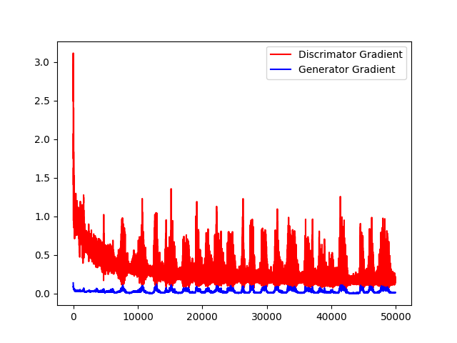
(a) MNIST

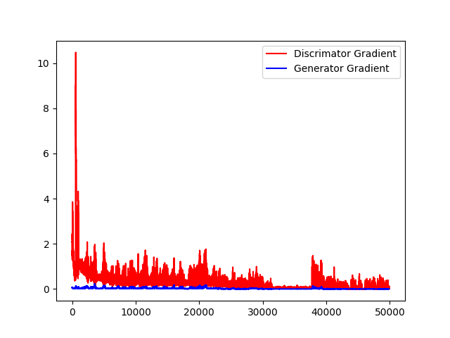
(b) Fashion-MNIST

Figure 1: We train GAN on the dataset MNIST and Fashion-MNIST. The two figures above show us the Frobenius norm of the gradients of discriminator and generator.

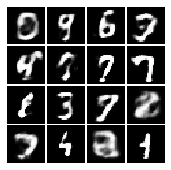
(a) MNIST figures

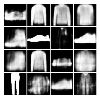
(b) Fashion-MNIST figures

Figure 2: After 50k iterations, we obtain these figures by using Adam. Despite its one-sided convergence, the min-max training actually succeeds.

This paper thus aims to explain this phenomenon by bridging the gap between theory and practice. On one hand, we understand under which conditions Adam-type optimization algorithms have provable convergence for min-max optimization. Towards this end, a recent work [LMR⁺20] designs two algorithms, Optimistic Stochastic Gradient (OSG) and Optimistic AdaGrad (OAdaGrad) for solving a class of non-convex non-concave min-max problems and gives theoretical guarantee on their convergence. [LMR⁺20] also proposes an open problem on the convergence proof of Adam-type algorithms, which is solved by this paper. On the other hand, we find that the MVI condition needed for our convergence proof does not practically hold for GANs. Instead, we propose the much milder one-sided MVI condition, which tends to hold practically and under which we provide the theoretical guarantee of the one-sided convergence of Adam-type algorithms in GANs’ training.

Despite some theoretical guarantee made on the convergence of Adam-type algorithms on convex concave or non-convex concave min-max optimization, in the non-convex non-concave setting which is most general, there is no theoretical guarantee on convergence. Comparatively speaking, proving the convergence of Adam-type algorithms is much more difficult since they use an empirical version of Momentum. Although it has been shown to perform well in practice, it is actually difficult to analyze theoretically. Even in the standard convex setting, proving the convergence of Adam-type algorithms [RKK18, ZCLG21] is much harder than other adaptive algorithms such as AdaGrad [DHS11]. Actually, the original version of Adam is known not to converge in convex settings. Therefore, to formally analyze the convergence of Adam-type algorithms in min-max optimization, we also consider a “theoretically correct” version of Adam, which is an analog of AMSGrad [RKK18]. In this paper, there are three main contributions, which are listed as follows:

• We analyze Extra Gradient AMSGrad, which is an Adam-type algorithm used for solving non-convex non-concave min-max optimization problems as well as GANs’ training. We prove that, under the assumption of standard MVI condition, the Extra Gradient AMSGrad algorithm provably converges to a $\varepsilon$-stationary point with $O(d\varepsilon^{-2})$ complexity in deterministic setting and $O(d\varepsilon^{-4})$ complexity in stochastic setting.

• Although the standard MVI condition above is a much milder assumption than convexity, we show by empirical experiments that MVI condition does not hold for GANs’ objective functions in reality. Instead, the one-sided MVI condition proposed by us tends to hold, which is the mildest assumption ever used in all the convergence proofs for min-max optimization. Under the the one-sided MVI condition, we modify the algorithm above by using dual rate decay, and theoretically prove its convergence rate.

• We conduct empirical experiments on GANs’ training by the Extra Gradient AMSGrad algorithm and the Extra Gradient AMSGrad with dual rate decay analyzed by us. We show that they have much better performance than the Stochastic Gradient Descent Ascent (SGDA) algorithm. Also, we empirically verify that our new one-sided MVI condition is indeed satisfied during GAN’s training while the previously proposed standard MVI condition is not, which makes the one-sided MVI condition much closer to reality than the standard version.

After achieving all these results, we are eventually able to understand the one-sided convergence of Adam-type algorithms in min-max optimization as well as in GAN’s training.

2 Background and Related Works

In this section, we will introduce the background knowledge as well as related works on the following three fields: adaptive gradient methods, min-max optimization, convergence properties of multiple algorithms for min-max optimization problems.

2.1 Adaptive Gradient Methods and Adam-type Methods

We consider the simplest 1-dimensional unconstrained minimization problem:

$$\min_{x\in\mathcal{D}\subseteq\mathbb{R}}f(x).$$

where $f:\mathcal{D}\rightarrow\mathbb{R}$ is a continuously differentiable function. As one of the most dominant algorithms on the optimization problem above, Stochastic Gradient Descent (SGD) was originally proposed by [GBC16], which has been both empirically and theoretically proved effective, especially when facing large datasets and complicated models. To further improve the performance of SGD, several adaptive variants of SGD have been proposed, such as RMSprop, Adam [KB15], AdaGrad [DHS11], AMSGrad [RKK18] and AdaDelta [Zei12]. Distinguished from the vanilla gradient descent or its stochastic version SGD, adaptive gradient methods use a coordinate-wise scaling of the updating direction and each iteration relies on the history information of past gradients. In AdaGrad, we use arithmetic average when adopting history gradient information of each iteration while in Adam, RMSprop etc., we use exponential moving average instead because its believed that the more current gradient information is more important. Although adaptive gradient methods and momentum based methods are two different routes on optimization, they are combined perfectly in Adam. Now we introduce the family of adaptive gradient methods and Adam-type, and all of them have the following form:

$$m_{t+1} =h_{t}\nabla f(x_{t})+r_{t}\cdot m_{t}$$

$$v_{t+1} =p_{t}(\nabla f(x_{t}))^{2}+q_{t}\cdot v_{t}$$

$$x_{t+1} =x_{t}-\lambda_{t}\cdot\frac{m_{t+1}}{\sqrt{v_{t+1}}+\varepsilon}.$$

Here, $f$ is the objective function to minimize. $h,r,p,q$ are scalars depending on $t$, $\lambda_{t}$ is the learning rate of the $t$-th iteration and $\varepsilon>0$ is a small constant used to protect the denominator from being close to 0. From the formula above, we see that the momentum $m_{t}$ is the weighted sum of the past gradients and $v_{t}$ is the weighted sum of the past squared gradients. When $h=1,r=0$, $m_{t+1}=\nabla f(x_{t})$ is just the current gradient.

We start with the original Adam.

• Adam:

  $$v_{t+1} =\alpha_{t}v_{t}+(1-\alpha_{t})(\nabla f(x_{t}))^{2}$$

  $$m_{t+1} =\beta_{t}m_{t}+(1-\beta_{t})\nabla f(x_{t})$$

  $$x_{t+1} =x_{t}-\lambda\cdot\frac{m_{t+1}}{\sqrt{v_{t+1}}+\varepsilon}.$$

  As we can see, Adam is a combination of adaptive gradient method and momentum method. Here, the momentum term is empirical, meaning that it does not coincide with acceleration techniques that are theoretically sound, which creates extra difficult for the analysis. In Adam, we have $h_{t}+r_{t}=p_{t}+q_{t}=1$. When the $\alpha_{t}=\alpha,\beta_{t}=\beta$ remains constant, there is a bias correction step where $v_{t+1}\leftarrow\frac{v_{t+1}}{1-\alpha^{t}}$ and $m_{t+1}\leftarrow\frac{m_{t+1}}{1-\beta^{t}}$. However, we may practically ignore this bias correction step since $\frac{1}{1-\alpha^{t}}$ and $\frac{1}{1-\beta^{t}}$ rapidly approach to 1.

• AMSGrad:

  $$\hat{v}_{t+1} =\alpha_{t}v_{t}+(1-\alpha_{t})(\nabla f(x_{t}))^{2}$$

  $$v_{t+1} =\max(v_{t},\hat{v}_{t+1})$$

  $$m_{t+1} =\beta_{t}v_{t}+(1-\beta_{t})\nabla f(x_{t})$$

  $$x_{t+1} =x_{t}-\lambda\cdot\frac{m_{t+1}}{\sqrt{v_{t+1}}+\varepsilon}.$$

  As we can see, AMSGrad is a variant of Adam. Their difference is that the velocity term $v_{t}$ keeps increasing in AMSGrad.

After showing the details of these traditional adaptive gradient methods and Adam-type methods, we introduce their convergence properties as well as their further variants. [RKK18] shows that Adam does not converge in some settings where large gradient information is rarely encountered and it will die out quickly because of the “short memory” property of the exponential moving average. However, under some conditions, the convergence proofs of adaptive gradient methods have been obtained. [BDMU18] proved the convergence rate of RMSprop and Adam when using deterministic gradients instead of stochastic gradients. [LO18] analyzed the convergence rate of AdaGrad under both convex and non-convex settings. All the papers above provide theoretical guarantee for the convergence of different types of adaptive gradient descent. After that, [CLSH19] extends Adam to a broader class of Adam-type algorithms and provides its convergence analysis for non-convex optimization problems. In order to combine the fast convergence of adaptive methods and better generalization with momentum based methods, a number of new algorithms are proposed, such as SC-AdaGrad / SC-RMSprop [MH17], AdamW [LH19], AdaBound [LXLS19] etc..

2.2 Min-max Optimization

In the min-max optimization problem, which is also known as saddle point problem, we have to solve:

$$\min_{x\in\mathcal{X}}\max_{y\in\mathcal{Y}}\phi(x,y),$$

where $\mathcal{X}\subseteq\mathbb{R}^{n_{1}},\mathcal{Y}\subseteq\mathbb{R}^{n_{2}}$, and $\phi:\mathcal{X}\times\mathcal{Y}\rightarrow\mathbb{R}$ is the objective function. When $\phi$ is convex on $x$ and concave on $y$, we call it a convex-concave min-max optimization. Otherwise, it’s a more general non-convex non-concave min-max optimization. For the brevity, we denote $z=(x,y)$ and $\mathcal{Z}=\mathcal{X}\times\mathcal{Y}\subseteq\mathbb{R}^{n_{1}+n_{2}}$. We also introduce our gradient vector field: $V(z)=(-\nabla_{x}\phi(x,y),\nabla_{y}\phi(x,y))$, which are the update directions on both sides. The goal of $[\mathrm{SP}]$ is to find a tuple $z^{*}=(x^{*},y^{*})$ such that $\phi(x^{*},y)\leqslant\phi(x^{*},y^{*})\leqslant\phi(x,y^{*})$ holds for $\forall x\in\mathcal{X},y\in\mathcal{Y}$, which is called the solution of $[\mathrm{SP}]$. If the inequality above only holds in the local neighbourhood of $z^{*}$, then $z^{*}$ can only be called a local solution. Notice that the necessary condition of being a solution (or even a local solution) is to be a stationary point of $\phi$, which means $V(z^{*})=0$. Furthermore, if $V$ is $C^{1}$, any local solution of $[\mathrm{SP}]$ must be stable, which means $\nabla_{xx}^{2}\phi(x^{*},y^{*})\succeq 0$ and $\nabla_{yy}^{2}\phi(x^{*},y^{*})\preceq 0$. Next, we will introduce several commonly-used algorithms which are designed to solve $[\mathrm{SP}]$.

Stochastic Gradient Descent Ascent (SGDA)

This is a simple extension of Stochastic Gradient Descent (SGD) algorithm for minimization problems [Joh59]. In the $t$-th iteration:

$$z_{t+1}=z_{t}+\gamma_{t}\cdot V(z_{t};\omega_{t}),$$

where $\omega_{1},\omega_{2},\cdots$ are the independent and identically distributed sequence of noises. $V(z,\omega)$ can be treated as a query to the stochastic first-order oracle (SFO). In each iteration of SGDA, we need to query SFO once. Notice that, we simultaneously update $x,y$ in each iteration of SGDA. Therefore, if we alternate the updates of $x$ and $y$, we obtain a variant of SGDA, which is named as the alternating stochastic gradient descent ascent (AltSGDA) algorithm:

$$x_{t+1} =x_{t}+\gamma_{t}\cdot V_{x}(x_{t},y_{t};\omega_{t}^{(1)})$$

$$y_{t+1} =y_{t}+\gamma_{t}\cdot V_{y}(x_{t+1},y_{t};\omega_{t}^{(2)})$$

Different from original SGDA, we have to make two queries to SFO in each iteration. One for $z_{t}=(x_{t},y_{t})$, and the other for the intermediate step $(x_{t+1},y_{t})$. Since original SGDA is not going to work even in the convex-concave setting (such as $\min_{x}\max_{y}f(x,y)=xy$), so researchers propose the following “theoretical correct modification”. Prior theoretical works [AZL21] that shows the global convergence of GANs training over real-world distributions also focus on SGDA due to its simplicity.

Stochastic Extra-gradient (SEG)

This is a different algorithm with the above SGDA, and it is originally proposed for solving the convex-concave setting of min-max optimization problems by [Kor76]. Given $z_{t}$ as a base, we take a virtual gradient descent ascent step and obtain a $\tilde{z}_{t}$, which can be treated as the shadow of $z_{t}$. Then we use the gradient at $z_{t}^{\prime}$ as the update direction of $z_{t}$. This process can be described as:

$$z_{t}^{\prime} =z_{t}+\gamma_{t}\cdot V(z_{t};\omega_{t}^{(1)})$$

$$z_{t+1} =z_{t}+\gamma_{t}\cdot V(z_{t}^{\prime};\omega_{t}^{(2)}).$$

In each iteration, we need to make two queries to the SFO. One for the base $z_{t}$ and the other for the shadow $z_{t}^{\prime}$. However, in the first step of $[\mathrm{SEG}]$, we can use the gradient at the previous shadow $z_{t-1}^{\prime}$ so that we only have to make only one query in each iteration and remember the query’s result of the previous step. This algorithm is called Optimistic Gradient or Popov’s Extra-gradient [Pop80] which can be described as:

$$z_{t}^{\prime} =z_{t}+\gamma_{t}\cdot V(z_{t-1}^{\prime};\omega_{t-1})$$

$$z_{t+1} =z_{t}+\gamma_{t}\cdot V(z_{t}^{\prime};\omega_{t}).$$

As a widely used algorithm, it has been applied in multiple works [DISZ18, MLZ⁺19]. Under some mild assumptions, convergence rates are proved by many theoretical works and we will summarize them in the next section.

2.3 Convergence Rates of Multiple Min-max Algorithms

In this section, we summarize the convergence rates of different algorithms as well as the assumptions needed. First, we start with the Mirror-Prox algorithm. [Nes07] provided the convergence guarantee of Mirror-Prox on in terms of the duality gap, and the rate is $O(1/T)$ where $T$ is the iteration number. As one of the most important algorithms for convex-concave optimization, [JNT11] introduced its stochastic version where only the stochastic first order oracle can be accessed, and also provided its convergence rate. When combined with [Dar83], we can conclude that the convergence rates for both deterministic and stochastic mirror-prox algorithm are optimal. When it comes to the more challenging non-convex non-concave min-max optimization, the two methods above are still useful. [DL15] showed that the deterministic extragradient method can converge to $\varepsilon$-first order stationary point with non-asymptotic guarantee. Another interesting algorithm Inexact Proximal Point (IPP) method [LLRY18], which is a stage-wise algorithm performs well under the condition that the objective function is weakly-convex weakly-concave. In each stage, we construct a strongly-convex strongly-concave sub-problem by adding quadratic regularizers. Then, by using stochastic algorithms, we can approximately solve the original problem. It’s known that IPP also has a convergence guarantee to first order stationary points. Also, [SRL18] proposed an alternating deterministic optimization algorithm, where multiple steps of gradient ascents are conducted before one gradient descent step. Therefore, we can approximately make sure that the max step always reaches near optimal. However, in order to guarantee its convergence to first order stationary point, we have to assume that the inner maximization problem satisfies PL condition [Pol69]. For the details of convergence rate, we summarize them into Table 1. Now we explain some terms in the table.

	Assumption	IC	Guarantee
OMD [DISZ18] (deterministic)	bilinear	N/A	asymptotic
OMD [MLZ+19] (stochastic)	coherence	N/A	asymptotic
OG [LMR+20] (stochastic)	MVI has solution	$\mathcal{O}(\varepsilon^{-4})$	$\varepsilon$-SP
OAdaGrad [LMR+20] (stochastic)	MVI has solution Bounded Cumulative Gradients	$\tilde{\mathcal{O}}\left((d/\varepsilon^{2})^{\frac{1}{1-\alpha}}\right)$	$\varepsilon$-SP
SEG [Kor76, IJOT17] (stochastic)	pseudo-monotonicity	$\mathcal{O}(\varepsilon^{-4})$	$\varepsilon$-SP
Extra-gradient [AMLG19] (deterministic)	strong-monotonicity	$\mathcal{O}(\log(1/\varepsilon))$	$\varepsilon$-optim
AltSGDA[GHP+19] (deterministic)	bilinear	$\mathcal{O}(\log(1/\varepsilon))$	$\varepsilon$-optim
IPP [LLRY18] (stochastic)	MVI has solution	$\mathcal{O}(\varepsilon^{-6})$	$\varepsilon$-SP
AvgPastExtraSGD [GBV+19] (stochastic)	monotonicity	$\mathcal{O}(\varepsilon^{-2})$	$\varepsilon$-DG
Extra Gradient AMSGrad (ours) (deterministic & stochastic)	MVI has solution	$\mathcal{O}(d\varepsilon^{-2})~{}\&$ $\mathcal{O}(d\varepsilon^{-4})$	$\varepsilon$-SP
Extra Gradient AMSGrad with Dual Rate Decay (ours) (deterministic & stochastic)	one-sided MVI has solution	$\tilde{\mathcal{O}}(d\varepsilon^{-2})~{}\&$ $\tilde{\mathcal{O}}(d\varepsilon^{-4})$	$\varepsilon$-SP

Table 1: Summary of different algorithms for min-max optimization. IC stands for iteration complexity, $\varepsilon$-SP stands for $\varepsilon$-first order stationary point, $\varepsilon$-DG stands for $\varepsilon$-duality gap, i.e. $\max_{y}\phi(x^{*},y)-\min_{x}\phi(x,y^{*})<\varepsilon$, and $\varepsilon$-optim stands for $\varepsilon$-close to the set of optimal solutions. The last two lines are algorithms proposed by us in this paper.

• Bilinear form is defined as:

  $$\min_{u\in\mathbb{R}^{p}}\max_{v\in\mathbb{R}^{q}}~{}u^{\top}Av+u^{\top}a+v^{\top}b,$$

  where $a\in\mathbb{R}^{p},b\in\mathbb{R}^{q}$ and $A\in\mathbb{R}^{p\times q}$. Bilinear setting is often used as toy examples in min-max optimization.

• Let $K:\mathbb{R}^{d}\rightarrow\mathbb{R}^{d}$ be an operator and $\mathcal{X}\subseteq\mathbb{R}^{d}$ is a closed convex domain. [HS66] proposed the Stampacchia Variational Inequality (SVI), which aims to find $z^{*}\in\mathcal{X}$, such that $\langle K(z^{*}),z-z^{*}\rangle\geqslant 0$ holds for all $z\in\mathcal{X}$. Similarly, [Min62] proposed the Minty Variational Inequality (MVI) problem, which aims to find $z^{*}\in\mathcal{X}$, such that $\langle K(z),z-z^{*}\rangle\geqslant 0$. In Table 1, the operator $K(z)=(\nabla_{x}\phi(x,y),-\nabla_{y}\phi(x,y))^{\top}=-V(z)$ with $z=(x,y)$.

3 Main Results

In this section, we introduce the main results of this paper. We focus on two algorithms: Extra Gradient AMSGrad (AMSGrad-EG) and Extra Gradient AMSGrad with Dual Rate Decay (AMSGrad-EG-DRD) which inherit the idea of OAdaGrad into Adam-type algorithms. With AMSGrad-EG, we can prove its first-order convergence under MVI condition. However, as we stated above, Adam does not perfectly converge in GANs’ training since MVI condition does not always hold practically for GANs’ objective functions. We bridge the gap by proposing one-sided MVI condition which is shown to be more likely to hold. Under this condition, we prove that Extra Gradient AMSGrad with Dual Rate Decay (AMSGrad-DRD) converges one-sidedly, which matches our experiment results.

3.1 Problem Setting and Assumptions

Throughout the paper, we analyze the min-max optimization problems (also known as saddle point problems):

$$\min_{x\in\mathcal{X}}\max_{y\in\mathcal{Y}}\phi(x,y),$$

where $\mathcal{X}\subseteq\mathbb{R}^{n_{1}},\mathcal{Y}\subseteq\mathbb{R}^{n_{2}}$, and $\phi:\mathcal{X}\times\mathcal{Y}\rightarrow\mathbb{R}$ is the objective function. We denote $z=(x,y)$ and $\mathcal{Z}=\mathcal{X}\times\mathcal{Y}$. First, we state some useful assumptions on $\phi(x,y)$:

Assumption 1.

(1) $V:=(-\nabla_{x}\phi,\nabla_{y}\phi)$ is $L$-Lipschitz continuous which means for $\forall z_{1},z_{2}\in\mathcal{Z}$, it holds that:

$$\|V(z_{1})-V(z_{2})\|_{2}\leqslant L\cdot\|z_{1}-z_{2}\|_{2}.$$

(2) The stochastic first order gradient oracle (SFO) is unbiased and has bounded variance:

$$\mathbb{E}[V(z;\xi)]=V(z)\text{~{}~{}and~{}~{}}\mathbb{E}\|V(z;\xi)-V(z)\|^{2}\leqslant\sigma^{2}.$$

(3) The Stochastic first-order Gradient Oracle (SFO) has bounded output: there exists $G>0$ and $\delta>0$ such that $\|V(z;\xi)\|_{2}\leqslant G$ and $\|V(z;\xi)\|_{\infty}\leqslant\delta$ almost surely holds.
(4) There exists a universal constant $D>0$, such that $\|z_{k}\|_{2}\leqslant D$ holds for all points $z_{k}$ on our trajectory and $\|z^{*}\|_{2}\leqslant D$. If the feasible set $\mathcal{Z}$ is bounded, then this assumption naturally holds.

Assumption 2 (Standard MVI condition).

The MVI of $-V(z)$ has a solution, which means there exists a $z^{*}$, such that:

$$\langle-V(z),z-z^{*}\rangle\geqslant 0\text{~{}holds for~{}}\forall z\in\mathcal{Z}$$

.

3.2 Extra Gradient AMSGrad (AMSGrad-EG)

In this section, we analyze the Extra Gradient AMSGrad (AMSGrad-EG) algorithm, which is used for non-convex non-concave min-max optimization, and we theoretically provide its convergence rate. So far, the convergence rate of Adam-type algorithms for min-max optimization has long been an open problem, and this work is the very first to obtain a related result. AMSGrad-EG algorithm is described as Algorithm 1.

Algorithm 1 Extra Gradient AMSGrad

Input: The initial state $z_{0}=m_{0}=v_{0}=0$, a constant learning rate $\eta$, momentum parameters $\beta_{1t},\beta_{2}$, a Stochastic First-order Oracle (SFO) $V(z;\xi)$, a sequence of batch sizes $\{M_{k}\}$.
 Output: $z_{t}$ where $t$ is uniformly chosen from $\{0,1,\ldots,N-1\}$.

1:  for $k=1,\ldots,N$ do

2:     (Gradient Evaluation 1) $g_{k-1}=\frac{1}{M_{k}}\sum_{i=1}^{M_{k}}V(z_{k-1};\xi_{k-1}^{i}).$

3:     (Momentum Update 1) $m_{k}=\beta_{1k}\hat{m}_{k-1}+(1-\beta_{1k})g_{k-1}.$

4:     (Velocity Update 1) $v_{k}=\max(\beta_{2}\hat{v}_{k-1}+(1-\beta_{2})g_{k-1}^{2},\hat{v}_{k-1}),~{}H_{k}=\delta I+\mathrm{Diag}(\sqrt{v_{k}}).$

5:     (Shadow Update) $\hat{z}_{k}=z_{k-1}+\eta\cdot H_{k}^{-1}m_{k}$.

6:     (Gradient Evaluation 2) $\hat{g}_{k}=\frac{1}{M_{k}}\sum_{i=1}^{M_{k}}V(\hat{z}_{k};\xi_{k}^{i})$.

7:     (Momentum Update 2) $\hat{m}_{k}=\beta_{1k}m_{k}+(1-\beta_{1k})\hat{g}_{k}.$

8:     (Velocity Update 2) $\hat{v}_{k}=\max(\beta_{2}v_{k}+(1-\beta_{2})\hat{g}_{k}^{2},v_{k}),~{}\hat{H}_{k}=\delta I+\mathrm{Diag}(\sqrt{\hat{v}_{k}})$

9:     (Real Update) $z_{k}=z_{k-1}+\eta\cdot\hat{H}_{k}^{-1}\hat{m}_{k}$.

10:  end for

Compared to the original Adam, we just add an extra-gradient technique and a taking-max process in velocity updates. It’s worth mentioned that if we delete the maximizing operation in velocity update steps, then this algorithm degenerates to Extra-Gradient Adam, since the largest difference between Adam and AMSGrad is that the latter one guarantees that the velocity term is non-decreasing.

Theorem 3.1 (Main Theorem 1).

For the AMSGrad-EG algorithm, given:

• the objective function $\phi(x,y):\mathbb{R}^{n_{1}+n_{2}}\rightarrow\mathbb{R}$ and $V(z)=(-\nabla_{x}\phi,\nabla_{y}\phi)$ that satisfy Assumption 1 and Assumption 2,

• the initial point $z_{0}\in\mathcal{Z}$, the iteration number $N$, a sequence of batch sizes $\{M_{k}\}$ and a constant learning rate $\eta\leqslant\frac{\delta}{3L}$,

the output of the algorithm satisfies the following inequality:

$$\mathbb{E}\|V(z)\|_{2}^{2} \leqslant\frac{1}{N}\left[\frac{6dD^{2}(\delta+G)^{2}}{\eta^{2}}+\frac{12dG^{2}(\delta+G)^{2}}{\delta^{2}}\right]+\frac{150\sigma^{2}(\delta+G)}{N\delta}\sum_{t=1}^{N}\frac{1}{M_{t}}$$

$$~{}~{}+\frac{48GD(\delta+G)}{N\eta}\sum_{t=1}^{N}\beta_{1t}+\frac{108\eta^{2}G^{2}(\delta+G)}{N\delta}\sum_{t=1}^{N}\beta_{1t}^{2}.$$

Here, we analyze the conclusion above on two sides: parameter choosing on $\beta_{1k}$ and on $M_{k}$.

• There are two practical ways to choose the parameter sequence $\{\beta_{1t}\}$: (1) $\beta_{1t}=\beta_{1}\cdot\lambda^{t-1}$ where $\beta_{1},\lambda\in(0,1)$ and (2) $\beta_{1t}=1/t$. In both settings, $\sum_{t=1}^{N}\beta_{1t}^{2}=\mathcal{O}(1)$ and $\sum_{t=1}^{N}\beta_{1t}=\widetilde{\mathcal{O}}(1)$. Therefore, we can conclude from Theorem 3.1 that: $\mathbb{E}\|V(z)\|_{2}^{2}\leqslant\mathcal{O}(d/N)+\mathcal{O}(1/N)\cdot\sum_{t=1}^{N}1/M_{t}$ holds after regarding $D,G,\delta,\eta$ as constants.

• When the batch sizes $M_{k}$ are constant, let $M_{k}=\Theta(1/\varepsilon^{2})$. To guarantee $\mathbb{E}\|V(z)\|_{2}^{2}\leqslant\varepsilon^{2}$, the total number of iterations should be $N=\mathcal{O}(d\varepsilon^{-2})$ and the total complexity is $\sum_{k=0}^{N}M_{k}=\mathcal{O}(d\varepsilon^{-4})$. When the batch sizes $M_{k}$ are increasing, let $M_{k}=k+1$. To guarantee $\mathbb{E}\|V(z)\|_{2}^{2}\leqslant\varepsilon^{2}$, the total number of iterations should be $N=\widetilde{\mathcal{O}}(d\varepsilon^{-2})$ and the total complexity is $\sum_{k=0}^{N}M_{k}=\widetilde{\mathcal{O}}(d^{2}\varepsilon^{-4})$. Obviously, using constant batch sizes obtains a better total complexity.

• In the deterministic setting, the first-order oracle directly outputs the accurate gradient $V(z;\xi)=V(z)$, which means $\sigma=0$. Theorem 3.1 leads to $\mathbb{E}\|V(z)\|_{2}^{2}\leqslant\mathcal{O}(d/N)$. To guarantee $\mathbb{E}\|V(z)\|_{2}^{2}\leqslant\varepsilon^{2}$, the total number of iterations should be $N=\mathcal{O}(d\varepsilon^{-2})$.

• In the AMSGrad-EG algorithm, the momentum term is a technical difficulty on the convergence proof. Proofs in the past works always use the MVI condition or convex condition like $\langle V(z_{k}),z_{k}-z^{*}\rangle\leqslant 0~{}\Rightarrow\langle g_{k},z_{k}-z^{*}\rangle\lessapprox 0$ to control the gradient norms. However, if we replace $g_{k}$ with the momentum term $m_{k}$, the inequality above will no longer hold, and then we have to find another way to control the upper bound of gradient norms. It’s also worth mentioned that our proof can’t be extended to Optimistic Adam (OAdam) since we need to guarantee that $H_{1}\preceq H_{2}\preceq\ldots$ in our proof. Actually, Adam may not even converge in convex case [RKK18].

• Comparison with OAdaGrad: [LMR⁺20] proposes the Optimistic AdaGrad (OAdaGrad) algorithm and gives a convergence analysis on under Assumption 1, 2 and Bounded Cumulative Gradient Assumption (which assumes the existence of a constant $0\leqslant\delta\leqslant 1/2$ such that the cumulative gradients are bounded as $\|\hat{g}_{1:k,i}\|_{2}\leqslant\delta k^{\alpha}$ for all $k$). Under these assumptions, they conclude that:

  $$\frac{1}{N}\sum_{k=1}^{N}\mathbb{E}\|V(z_{k})\|_{H_{k-1}^{-1}}^{2}\leqslant\mathcal{O}(1/N^{1-\alpha}).$$

  On one hand, notice that $\frac{1}{N}\sum_{k=1}^{N}\mathbb{E}\|V(z_{k})\|_{H_{k-1}^{-1}}^{2}$ is the average of the norms of $V(z_{k})$. However, the norm keeps changing. Since $H_{k-1}^{-1}$ keeps decreasing and may limit to 0 as $k\rightarrow\infty$, its unclear what is the real convergence rate in terms of the size of the gradient. It would be more convincing if we can upper bound the average of constant norms like $\frac{1}{N}\sum_{k=1}^{N}\mathbb{E}\|V(z_{k})\|_{2}^{2}$. On the other hand, the Bounded Cumulative Assumption though widely used in related papers [ZTY⁺18, RKK18, DHS11], is actually a very strong assumption: Under this assumption, it holds that $\|\hat{g}_{1:k,i}\|_{2}\leqslant\delta k^{\alpha}$, which naturally leads to:

  $$\frac{1}{N}\sum_{k=1}^{N}\mathbb{E}\|V(z_{k})\|_{2}^{2}\leqslant\frac{1}{N}\sum_{k=1}^{N}\mathbb{E}\|\hat{g}_{k}\|_{2}^{2}\leqslant\mathcal{O}\left(\frac{d}{N^{1-2\alpha}}\right).$$

  It causes a possible circularity about the argument. In this paper, we successfully overcome these two shortcomings.

Standard MVI condition and one-sided MVI

From Table 1, we can see that many related convergence proofs rely on assuming the MVI condition of $-V(z)$, which means $\langle V(z),z-z^{*}\rangle\leqslant 0~{}~{}\forall z\in\mathcal{Z}$. Although MVI condition is theoretically known to be true in many standard supervised deep learning settings [LY17, KLY18, AZL20a, AL20, LMZ18, LMZ20, AZL20b, AZL19]. However, this is a rather unrealistic assumption for GANs: In some practical scenarios such as DCGAN [RMC15], it is unclear whether the training objective can satisfy the MVI condition: While the generator might have a consistent gradient direction towards the optimal generator (which is the one that generates the target distribution), it is very unlikely that there is a “optimal discriminator” where the discriminator’s gradient is pointing to through the course of the training. Indeed, different generator should in principle requires different discriminator to discriminate it from the target distribution, which precludes the MVI condition to hold on $y$.

Also, in practical scenarios like GAN, we only care about the min-variable $x$ (which refers to the generator of GAN), and the optimally of $y$ is not needed. Therefore, in the following part, we propose a weaker version of MVI condition, which is the one-sided MVI condition. Recall that $z=(x,y),z^{*}=(x^{*},y^{*})$ where $x\in\mathcal{X},y\in\mathcal{Y},\mathcal{Z}=\mathcal{X}\times\mathcal{Y}$, and $V(z)=(-\nabla_{x}\phi(z),\nabla_{y}\phi(z)):=(V_{x}(z),V_{y}(z))$. Then, the one-sided MVI condition implies that $\langle V_{x}(z),x-x^{*}\rangle\leqslant 0~{}~{}~{}\forall z\in\mathcal{Z}$, which means for any $y\in\mathcal{Y}$, the $x$-part of function $V$, $-V(\cdot,y)$ satisfies the MVI condition. Now we empirically verify that one-sided MVI is more likely to hold in practice in some simple applications of GANs. For $z,z^{*}\in\mathcal{Z}$:

$$\langle-V(z),z-z^{*}\rangle=\langle-V_{x}(z),x-x^{*}\rangle+\langle-V_{y}(z),y-y^{*}\rangle,$$

where $z=(x,y),z^{*}=(x^{*},y^{*})$. We call the three terms above as total MVI, $x$-sided MVI and $y$-sided MVI respectively. Assumption 2 requires total MVI to be non-negative, and Assumption 3 requires $x$-sided MVI to be non-negative. After training Wasserstein GAN on the MNIST/Fashion MNIST dataset with AMSGrad-EG optimizer, we denote $z_{k}:=(x_{k},y_{k})$ as the value of $z$ at the $k$-th iteration, and $z^{*}:=(x^{*},y^{*})$ as the value of $z$ at the last iteration. In the following Figure 3, we plot the total MVI values $\langle-V(z_{k}),z_{k}-z^{*}\rangle$, $x$-sided MVI values $\langle-V_{x}(z_{k}),x_{k}-x^{*}\rangle$, and $y$-sided MVI values $\langle-V_{y}(z_{k}),y_{k}-y^{*}\rangle$ along the training trajectory. We can see that $x$-sided MVI stays positive while the total MVI does not, which means the one-sided MVI condition proposed in Assumption 3 is more realistic than the original MVI condition in Assumption 2.

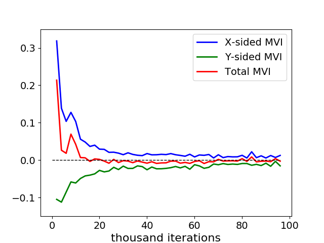
(a) MNIST

(b) Fashion MNIST

Figure 3: This figure shows the MVI values along the training trajectory. As we can see, the blue curve stays above $x$ axis in both experiments while the red curve does not. Since we use non-linear activations in the network architecture, this result is exciting. It’s safe to say that the one-sided MVI condition proposed by us fits the reality since the $x$-sided MVI keeps positive.

Under the one-sided MVI condition, we prove in our next theorem that, the conclusion of Theorem 3.1 still holds once we slightly modify AMSGrad-EG to AMSGrad with Extra-Gradient & Dual Rate Decay (AMSGrad-EG-DRD). To the best of our knowledge, this is a convergence guarantee of an adaptive min-max algorithm with the weakest assumption ever needed. In the next section, we introduce the AMSGrad-EG-DRD algorithm and its convergence property.

3.3 Extra Gradient AMSGrad with Dual Rate Decay

Now, we write down the one-sided MVI condition introduced above into the following Assumption 3, which is the weakest assumption ever needed to obtain a convergence guarantee in min-max optimization.

Assumption 3 (One-sided MVI condition).

The one-sided MVI of $-V(z)$ has a solution, which means there exists a $z^{*}=(x^{*},y^{*})\in\mathcal{Z}$, such that:

$$\langle-V_{x}(z),x-x^{*}\rangle\geqslant 0\text{~{}holds for~{}}\forall z=(x,y)\in\mathcal{Z}.$$

After slightly modifying AMSGrad-EG with a $\mathcal{O}(1/\sqrt{k})$ dual rate decay, we obtain the Algorithm 2. Here, we denote $m_{k}=(m_{k}^{x},m_{k}^{y})$ and $H_{k}=\mathrm{Diag}(H_{k}^{x},H_{k}^{y})$ where $m_{k}^{x}\in\mathbb{R}^{n_{1}},m_{k}^{y}\in\mathbb{R}^{n_{2}},H_{k}^{x}\in\mathbb{R}^{n_{1}}\times\mathbb{R}^{n_{1}},H_{k}^{y}\in\mathbb{R}^{n_{2}}\times\mathbb{R}^{n_{2}}$.

Algorithm 2 Extra Gradient AMSGrad with Dual Rate Decay

Input: The initial state $z_{0}=m_{0}=v_{0}=0$, a constant learning rate $\eta$, a Stochastic First-order Oracle (SFO) $V(z;\xi)$, momentum parameters $\beta_{1t},\beta_{2}$, a sequence of batch sizes $\{M_{k}\}$.
 Output: $z_{t}$ with $t$ uniformly chosen from $\{0,1,\ldots,N-1\}$.

1:  for $k=1,\ldots,N$ do

2:     (Gradient Evaluation 1) $g_{k-1}=\frac{1}{m}\sum_{i=1}^{m}V(z_{k-1};\xi_{k-1}^{i}).$

3:     (Momentum Update 1)$m_{k}=\beta_{1k}\hat{m}_{k-1}+(1-\beta_{1k})g_{k-1}$

4:     (Velocity Update 1) $v_{k}=\max(\beta_{2}\hat{v}_{k-1}+(1-\beta_{2})g_{k-1}^{2},\hat{v}_{k-1}),~{}H_{k}=\delta I+\mathrm{Diag}(\sqrt{v_{k}}).$

5:     (Shadow Update) $\hat{x}_{k}=x_{k-1}+\eta\cdot\left(H_{k}^{x}\right)^{-1}m_{k}^{x},$$\hat{y}_{k}=y_{k-1}+\frac{\eta}{\sqrt{k}}\left(H_{k}^{y}\right)^{-1}m_{k}^{y},~{}\hat{z}_{k}=(\hat{x}_{k},\hat{y}_{k}).$

6:     (Gradient Evaluation 2) $\hat{g}_{k}=\frac{1}{M_{k}}\sum_{i=1}^{M_{k}}V(\hat{z}_{k};\xi_{k}^{i})$.

7:     (Momentum Update 2) $\hat{m}_{k}=\beta_{1k}m_{k}+(1-\beta_{1k})\hat{g}_{k}.$

8:     (Velocity Update 2) $\hat{v}_{k}=\max(\beta_{2}v_{k}+(1-\beta_{2})\hat{g}_{k}^{2},v_{k}),~{}\hat{H}_{k}=\delta I+\mathrm{Diag}(\sqrt{\hat{v}_{k}})$

9:     (Real Update) $z_{k}=z_{k-1}+\eta\cdot\hat{H}_{k}^{-1}\hat{m}_{k}$.

10:     (Real Update) $x_{k}=x_{k-1}+\eta\cdot\left(\hat{H}_{k}^{x}\right)^{-1}\hat{m}_{k}^{x},$$y_{k}=y_{k-1}+\frac{\eta}{\sqrt{k}}\left(\hat{H}_{k}^{y}\right)^{-1}\hat{m}_{k}^{y},~{}z_{k}=(x_{k},y_{k}).$

11:  end for

Theorem 3.2 (Main Theorem 2).

For the AMSGrad with Extra-Gradient and Dual Rate Decay (AMSGrad-EG-DRD) algorithm, given:

• the objective function $\phi(x,y):\mathbb{R}^{n_{1}+n_{2}}\rightarrow\mathbb{R}$ and $V(z)=(-\nabla_{x}\phi,\nabla_{y}\phi):=(V_{x}(z),V_{y}(z))$ that satisfy Assumption 1 and Assumption 3,

• the initial point $z_{0}\in\mathcal{Z}$, the iteration number $N$, a sequence of batch sizes $\{M_{k}\}$ and a constant learning rate $\eta\leqslant\frac{\delta}{3L}$,

the output of the algorithm satisfies the following inequality:

$$\mathbb{E}\|V_{x}(z)\|_{2}^{2}\leqslant\frac{(15+3\log N)dG^{2}(\delta+G)^{2}}{N\delta^{2}}+\frac{6dD^{2}(\delta+G)^{2}}{N\eta^{2}}+\frac{150\sigma^{2}(\delta+G)}{N\delta}\sum_{t=1}^{N}\frac{1}{M_{t}}$$

$$~{}~{}+\frac{48GD(\delta+G)}{N\eta}\sum_{t=1}^{N}\beta_{1t}+\frac{108\eta^{2}G^{2}(\delta+G)}{N\delta}\sum_{t=1}^{N}\beta_{1t}^{2}.$$

Similar to Theorem 3.1, in the deterministic setting where $\sigma=0$, the total complexity is $\widetilde{\mathcal{O}}(d\varepsilon^{-2})$. In the stochastic setting, we have: $\mathbb{E}\|V_{x}(z)\|_{2}^{2}\leqslant\widetilde{\mathcal{O}}(d/N)+\mathcal{O}(1/N)\cdot\sum_{t=1}^{N}1/M_{t}.$ When we use constant batch sizes $M_{k}=\Theta(1/\varepsilon^{2})$, iteration number $N$ should be $\widetilde{\mathcal{O}}(d\varepsilon^{-2})$ in order to guarantee that $\mathbb{E}\|V_{x}(z)\|_{2}^{2}\leqslant\varepsilon^{2}$. So the total complexity should be $\widetilde{\mathcal{O}}(d\varepsilon^{-4})$.

4 Experimental Results

In this section, we use experiments to verify the effectiveness of AMSGrad-EG and AMSGrad-EG-DRD algorithms by applying Wasserstein GAN [ACB17] on the MNIST [LBBH98] and Fashion MNIST [XRV17] datasets in our experiments. More experiments will be shown in the appendix. The architectures of discriminator and generator are set to be MLP. The layer widths of generator MLP are 100, 128, 784 (figure’s dimension) and the layer widths of discriminator MLP are 784, 128, 1. We set batch sizes as 64, learning rate as $1e$-4 and we compare AMSGrad-EG, AMSGrad-EG-DRD and SGDA by drawing their generated figures after 10k, 20k, 50k iterations in the following Figures 4 and 5. We use the Tensorflow framework [ABC⁺16] to complete our experiments. As a result, unlike the non-adaptive SGDA algorithm, the two algorithms proposed by us perform better than the non-adaptive SGDA and their generated figures are almost real, which shows their effectiveness.

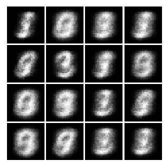
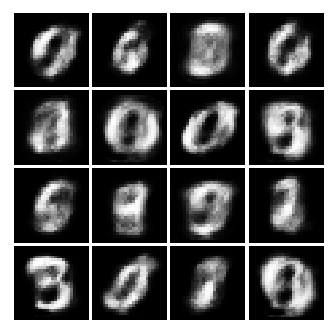
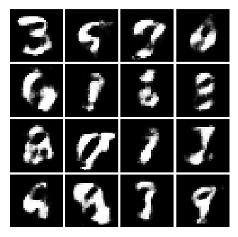
(a) AMSGrad-EG

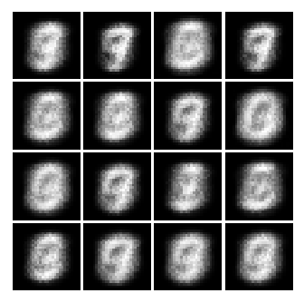
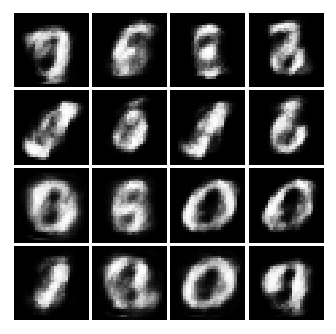
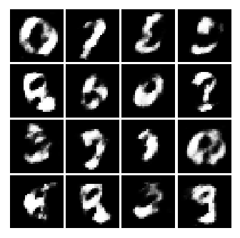
(b) AMSGrad-EG-DRD

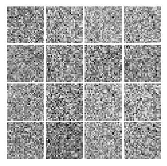
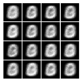
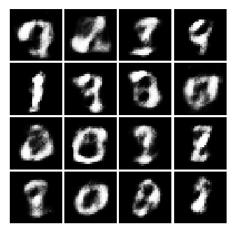
(c) SGDA

Figure 4: These are the generated MNIST figures by the three algorithms after 10k, 20k, 50k iterations.

(a) AMSGrad-EG

(b) AMSGrad-EG-DRD

(c) SGDA

Figure 5: These are the generated Fashion MNIST figures by the three algorithms after 10k, 20k, 50k iterations.

Appendix A Proof for the Convergence of AMSGrad-EG

We recall that in the $t$-th iteration of Extra-Gradient AMSGrad, our update is as follows:

$$m_{t} =\beta_{1t}\hat{m}_{t-1}+(1-\beta_{1t})g_{t-1},~{}v_{t}=\max(\beta_{2}\hat{v}_{t-1}+(1-\beta_{2})g_{t-1}^{2},\hat{v}_{t-1})$$ (1)

$$H_{t} =\delta I+\mathrm{Diag}(\sqrt{v_{t}}),~{}\hat{z}_{t}=z_{t-1}+\eta\cdot H_{t}^{-1}m_{t}$$

$$\hat{m}_{t} =\beta_{1t}m_{t}+(1-\beta_{1t})\hat{g}_{t},~{}\hat{v}_{t}=\max(\beta_{2}v_{t}+(1-\beta_{2})\hat{g}_{t}^{2},v_{t})$$

$$\hat{H}_{t} =\delta I+\mathrm{Diag}(\sqrt{\hat{v}_{t}}),~{}z_{t}=z_{t-1}+\eta\cdot\hat{H}_{t}^{-1}\hat{m}_{t}.$$

Now we begin to prove Theorem 3.1 (Main Theorem 1). Before that, we prove that as the weighted sum of stochastic gradient, the momentum terms $m_{t}$, $\hat{m}_{t}$ are also contained in $l_{2}$ ball with radius $G$.

Lemma A.1.

There exist upper bounds for both velocity terms $v_{t},\hat{v}_{t}$ and momentum terms $m_{t},\hat{m}_{t}$:
(1) For $\forall t\in\mathbb{N}$, almost surely, the momentum terms $\|m_{t}\|_{2}\leqslant G,\|\hat{m}_{t}\|_{2}\leqslant G$.
(2) For $\forall t\in\mathbb{N}$, almost surely, the velocity terms $|v_{t,i}|\leqslant G^{2},|\hat{v}_{t,i}|\leqslant G^{2}$ hold for $\forall i\in[d]$.

Proof of Lemma A.1.

Actually, this lemma can be simply proved by using the method of induction. Since we’ve assumed that $\|V(z)\|_{2}\leqslant G$ almost surely holds for $z\in\mathcal{Z}=\mathbb{R}^{d}$, so $\|g_{t}\|_{2}\leqslant G$ and $\|\hat{g}_{t}\|_{2}\leqslant G$ almost surely holds. Therefore, by knowing that $m_{0}=\hat{m}_{0}=0~{}\Rightarrow~{}0=\|m_{0}\|_{2}=\|\hat{m}_{0}\|\leqslant G$ and once $\|m_{k-1}\|_{2}\leqslant G,\|\hat{m}_{k-1}\|_{2}\leqslant G$, we have:

$$\|m_{k}\|_{2} =\|\beta_{1k}\hat{m}_{k-1}+(1-\beta_{1k})g_{k-1}\|_{2}\leqslant\beta_{1k}\|\hat{m}_{k-1}\|_{2}+(1-\beta_{1k})\|g_{k-1}\|_{2}\leqslant(1-\beta_{1k})G+\beta_{1k}G=G$$

$$\|\hat{m}_{k}\|_{2} =\|\beta_{1k}m_{k}+(1-\beta_{1k})\hat{g}_{k}\|_{2}\leqslant\beta_{1k}\|m_{k}\|_{2}+(1-\beta_{1k})\|\hat{g}_{k}\|_{2}\leqslant(1-\beta_{1k})G+\beta_{1k}G=G.$$

Similarly, the upper bound for velocity terms can also be easily proved.

∎

Lemma A.2.

$$\|z_{t}-z^{*}\|_{\hat{H}_{t}}^{2}\leqslant\|z_{t-1}-z^{*}\|_{\hat{H}_{t}}^{2}-\|z_{t-1}-\hat{z}_{t}\|_{\hat{H}_{t}}^{2}+\|\hat{z}_{t}-z_{t}\|_{\hat{H}_{t}}^{2}+2\langle\eta\cdot\hat{\varepsilon}_{t},\hat{z}_{t}-z^{*}\rangle+8\eta\beta_{1t}GD.$$

Here, $\hat{\varepsilon}_{t}=\hat{g}_{t}-V(\hat{z}_{t})=\frac{1}{M_{t}}\sum_{i=1}^{M_{t}}V(\hat{z}_{t};\hat{\xi}_{i})-V(\hat{z}_{t})$.

Proof of Lemma A.2.

According to the update rules:

$$\|z_{t}-z^{*}\|_{\hat{H}_{t}}^{2} =\|z_{t-1}+\eta\cdot\hat{H}_{t}^{-1}\hat{m}_{t}-z^{*}\|_{\hat{H}_{t}}^{2}$$

$$=\|z_{t-1}+\eta\cdot\hat{H}_{t}^{-1}\hat{m}_{t}-z^{*}\|_{\hat{H}_{t}}^{2}-\|z_{t-1}+\eta\cdot\hat{H}_{t}^{-1}\hat{m}_{t}-z_{t}\|_{\hat{H}_{t}}^{2}$$

$$=\|z_{t-1}-z^{*}\|_{\hat{H}_{t}}^{2}-\|z_{t-1}-z_{t}\|_{\hat{H}_{t}}^{2}+2\langle\eta\cdot\hat{m}_{t},z_{t}-z^{*}\rangle$$

$$=\|z_{t-1}-z^{*}\|_{\hat{H}_{t}}^{2}-\|z_{t-1}-\hat{z}_{t}+\hat{z}_{t}-z_{t}\|_{\hat{H}_{t}}^{2}+2\langle\eta\cdot\hat{m}_{t},z_{t}-\hat{z}_{t}\rangle+2\langle\eta\cdot\hat{m}_{t},\hat{z}_{t}-z^{*}\rangle$$

$$=\|z_{t-1}-z^{*}\|_{\hat{H}_{t}}^{2}-\|z_{t-1}-\hat{z}_{t}\|_{\hat{H}_{t}}^{2}-\|\hat{z}_{t}-z_{t}\|_{\hat{H}_{t}}^{2}-2\langle\hat{H}_{t}(z_{t-1}-\hat{z}_{t}),\hat{z}_{t}-z_{t}\rangle$$

$$~{}~{}~{}~{}+2\langle\eta\cdot\hat{m}_{t},z_{t}-\hat{z}_{t}\rangle+2\langle\eta\cdot\hat{m}_{t},\hat{z}_{t}-z^{*}\rangle$$

$$=\|z_{t-1}-z^{*}\|_{\hat{H}_{t}}^{2}-\|z_{t-1}-\hat{z}_{t}\|_{\hat{H}_{t}}^{2}-\|\hat{z}_{t}-z_{t}\|_{\hat{H}_{t}}^{2}+2\langle\eta\cdot\hat{m}_{t},\hat{z}_{t}-z^{*}\rangle$$

$$~{}~{}~{}~{}+2\langle z_{t}-\hat{z}_{t},\hat{H}_{t}(z_{t-1}-\hat{z}_{t}+\eta\cdot\hat{H}_{t}^{-1}\hat{m}_{t})\rangle$$

$$=\|z_{t-1}-z^{*}\|_{\hat{H}_{t}}^{2}-\|z_{t-1}-\hat{z}_{t}\|_{\hat{H}_{t}}^{2}-\|\hat{z}_{t}-z_{t}\|_{\hat{H}_{t}}^{2}+2\langle\eta\cdot\hat{m}_{t},\hat{z}_{t}-z^{*}\rangle$$

$$~{}~{}~{}~{}+2\langle z_{t}-\hat{z}_{t},\hat{H}_{t}(z_{t}-\hat{z}_{t})\rangle$$

$$=\|z_{t-1}-z^{*}\|_{\hat{H}_{t}}^{2}-\|z_{t-1}-\hat{z}_{t}\|_{\hat{H}_{t}}^{2}+\|\hat{z}_{t}-z_{t}\|_{\hat{H}_{t}}^{2}+2\langle\eta\cdot\hat{m}_{t},\hat{z}_{t}-z^{*}\rangle$$

Notice that $\hat{g}_{t}=V(\hat{z}_{t})+\hat{\varepsilon}_{t}$. Since $z^{*}$ is a solution of MVI which means $\langle V(z),z-z^{*}\rangle\leqslant 0$ holds for $\forall z\in\mathcal{Z}$, so $\langle V(\hat{z}_{t}),\hat{z}_{t}-z^{*}\rangle\leqslant 0$. Therefore:

$$\langle\eta\cdot\hat{m}_{t},\hat{z}_{t}-z^{*}\rangle =\langle\eta\cdot(\beta_{1t}m_{t}+(1-\beta_{1t})\hat{g}_{t}),\hat{z}_{t}-z^{*}\rangle\leqslant\langle\eta\cdot\hat{g}_{t},\hat{z}_{t}-z^{*}\rangle+\langle\eta\cdot\beta_{1t}(m_{t}-\hat{g}_{t}),\hat{z}_{t}-z^{*}\rangle$$

$$\leqslant\langle\eta\cdot(V(\hat{z}_{t})+\hat{\varepsilon}_{t}),\hat{z}_{t}-z^{*}\rangle+\eta\beta_{1t}\cdot\|m_{t}-\hat{g}_{t}\|_{2}\cdot\|\hat{z}_{t}-z^{*}\|_{2}$$

$$\overset{(a)}{\leqslant}\langle\eta\hat{\varepsilon}_{t},\hat{z}_{t}-z^{*}\rangle+4\eta\beta_{1t}GD.$$

Here, $(a)$ holds because $\|m_{t}-\hat{g}_{t}\|_{2}\leqslant\|m_{t}\|_{2}+\|\hat{g}_{t}\|_{2}\leqslant 2G$, $\|\hat{z}_{t}-z^{*}\|_{2}\leqslant 2D$ and by using MVI property, $\langle V(\hat{z}_{t}),\hat{z}_{t}-z^{*}\rangle\leqslant 0$.
Combine it with the inequality above, we obtain that:

$$\|z_{t}-z^{*}\|_{\hat{H}_{t}}^{2}\leqslant\|z_{t-1}-z^{*}\|_{\hat{H}_{t}}^{2}-\|z_{t-1}-\hat{z}_{t}\|_{\hat{H}_{t}}^{2}+\|\hat{z}_{t}-z_{t}\|_{\hat{H}_{t}}^{2}+2\langle\eta\cdot\hat{\varepsilon}_{t},\hat{z}_{t}-z^{*}\rangle+8\eta\beta_{1t}GD.$$

which comes to our conclusion. ∎

In the lemma above, $\langle\eta\cdot\hat{\varepsilon}_{t},\hat{z}_{t}-z^{*}\rangle$ has zero mean. So it can be ignoring when taking expectation. Next, we upper bound the $\|\hat{z}_{t}-z_{t}\|_{\hat{H}_{t}}^{2}$ term.

Lemma A.3.

$$\|\hat{z}_{t}-z_{t}\|_{\hat{H}_{t}}^{2} \leqslant 2\eta^{2}\cdot\|(\hat{H}_{t}^{-1}-H_{t}^{-1})m_{t}\|_{\hat{H}_{t}}^{2}+\frac{16\eta^{2}G^{2}\beta_{1t}^{2}}{\delta}+\frac{12\eta^{2}L^{2}}{\delta^{2}}\cdot\|\hat{z}_{t}-z_{t-1}\|_{\hat{H}_{t}}^{2}$$

$$~{}~{}~{}~{}+12\eta^{2}\cdot\left(\|\hat{\varepsilon}_{t}\|_{\hat{H}_{t}^{-1}}^{2}+\|\varepsilon_{t-1}\|_{H_{t}^{-1}}^{2}\right).$$

Here, $\varepsilon_{t-1}=g_{t-1}-V(z_{t-1})$ and $\hat{\varepsilon}_{t}=\hat{g}_{t}-V(\hat{z}_{t})$.

Proof of Lemma A.3.

According to the update rules (1), we know that $z_{t}-\hat{z}_{t}=\eta\cdot(\hat{H}_{t}^{-1}\hat{m}_{t}-H_{t}^{-1}m_{t})$. Therefore, we upper bound the term $\|\hat{z}_{t}-z_{t}\|_{\hat{H}_{t}}^{2}$ as follows:

$$\|\hat{z}_{t}-z_{t}\|_{\hat{H}_{t}}^{2} =\eta^{2}\cdot\|\hat{H}_{t}^{-1}\hat{m}_{t}-H_{t}^{-1}m_{t}\|_{\hat{H}_{t}}^{2}=\eta^{2}\cdot\|\hat{H}_{t}^{-1}(\hat{m}_{t}-m_{t})+(\hat{H}_{t}^{-1}-H_{t}^{-1})m_{t}\|_{\hat{H}_{t}}^{2}$$

$$\leqslant 2\eta^{2}\cdot\left(\|\hat{m}_{t}-m_{t}\|_{\hat{H}_{t}^{-1}}^{2}+\|(\hat{H}_{t}^{-1}-H_{t}^{-1})m_{t}\|_{\hat{H}_{t}}^{2}\right)$$

$$\overset{(a)}{=}2\eta^{2}\cdot\|(\hat{H}_{t}^{-1}-H_{t}^{-1})m_{t}\|_{\hat{H}_{t}}^{2}+2\eta^{2}\cdot\|\beta_{1t}(m_{t}-\hat{m}_{t-1})+(1-\beta_{1t})(\hat{g}_{t}-g_{t-1})\|_{\hat{H}_{t}^{-1}}^{2}$$

$$\overset{(b)}{\leqslant}2\eta^{2}\cdot\|(\hat{H}_{t}^{-1}-H_{t}^{-1})m_{t}\|_{\hat{H}_{t}}^{2}+4\eta^{2}\left(\beta_{1t}^{2}\|m_{t}-\hat{m}_{t-1}\|_{\hat{H}_{t}^{-1}}^{2}+(1-\beta_{1t})^{2}\|\hat{g}_{t}-g_{t-1}\|_{\hat{H}_{t}^{-1}}^{2}\right)$$

$$\overset{(c)}{\leqslant}2\eta^{2}\cdot\|(\hat{H}_{t}^{-1}-H_{t}^{-1})m_{t}\|_{\hat{H}_{t}}^{2}+\frac{16\eta^{2}\beta_{1t}^{2}G^{2}}{\delta}+4\eta^{2}\|\hat{g}_{t}-g_{t-1}\|_{\hat{H}_{t}^{-1}}^{2}$$

$$\overset{(d)}{=}2\eta^{2}\cdot\|(\hat{H}_{t}^{-1}-H_{t}^{-1})m_{t}\|_{\hat{H}_{t}}^{2}+\frac{16\eta^{2}G^{2}\beta_{1t}^{2}}{\delta}+4\eta^{2}\|V(\hat{z}_{t})-V(z_{t-1})+\hat{\varepsilon}_{t}-\varepsilon_{t-1}\|_{\hat{H}_{t}^{-1}}^{2}$$

$$\overset{(e)}{\leqslant}2\eta^{2}\cdot\|(\hat{H}_{t}^{-1}-H_{t}^{-1})m_{t}\|_{\hat{H}_{t}}^{2}+\frac{16\eta^{2}G^{2}\beta_{1t}^{2}}{\delta}+12\eta^{2}\cdot\|V(\hat{z}_{t})-V(z_{t-1})\|_{\hat{H}_{t}^{-1}}^{2}$$

$$~{}~{}~{}~{}+12\eta^{2}\cdot\left(\|\hat{\varepsilon}_{t}\|_{\hat{H}_{t}^{-1}}^{2}+\|\varepsilon_{t-1}\|_{\hat{H}_{t}^{-1}}^{2}\right)$$

$$\overset{(f)}{\leqslant}2\eta^{2}\cdot\|(\hat{H}_{t}^{-1}-H_{t}^{-1})m_{t}\|_{\hat{H}_{t}}^{2}+\frac{16\eta^{2}G^{2}\beta_{1t}^{2}}{\delta}+\frac{12\eta^{2}L^{2}}{\delta^{2}}\cdot\|\hat{z}_{t}-z_{t-1}\|_{\hat{H}_{t}}^{2}$$

$$~{}~{}~{}~{}+12\eta^{2}\cdot\left(\|\hat{\varepsilon}_{t}\|_{\hat{H}_{t}^{-1}}^{2}+\|\varepsilon_{t-1}\|_{H_{t}^{-1}}^{2}\right)$$

Here, $(a)$ holds because $m_{t}=\beta_{1t}\hat{m}_{t-1}+(1-\beta_{1t})g_{t-1},\hat{m}_{t}=\beta_{1t}m_{t}+(1-\beta_{1t})\hat{g}_{t}$, and then:

$$\hat{m}_{t}-m_{t}=\beta_{1t}(m_{t}-\hat{m}_{t-1})+(1-\beta_{1t})(\hat{g}_{t}-g_{t-1}).$$

$(b)$ holds because $\|a+b\|_{C}^{2}\leqslant(\|a\|_{C}+\|b\|_{C})^{2}\leqslant 2(\|a\|_{C}^{2}+\|b\|_{C}^{2})$ and $(e)$ holds because of the similar reason: $\|x+y+z\|_{C}^{2}\leqslant(\|x\|_{C}+\|y\|_{C}+\|z\|_{C})^{2}\leqslant 3(\|x\|_{C}^{2}+\|y\|_{C}^{2}+\|z\|_{C}^{2})$. $(c)$ holds because $(1-\beta_{1t})^{2}<1$ and

$$\|m_{t}-\hat{m}_{t-1}\|_{\hat{H}_{t}^{-1}}^{2}\leqslant\frac{\|m_{t}-\hat{m}_{t-1}\|^{2}}{\delta}\leqslant\frac{4G^{2}}{\delta}.$$

$(d)$ holds because $\hat{g}_{t}=V(\hat{z}_{t})+\hat{\varepsilon}_{t}$ and $g_{t-1}=V(z_{t-1})+\varepsilon_{t-1}$. $(f)$ holds because of the following fact:

$$\delta I=H_{0}\preceq\hat{H}_{0}\preceq H_{1}\preceq\hat{H}_{1}\preceq\ldots\preceq\hat{H}_{N}\preceq\ldots,$$

or equivalently:

$$\frac{1}{\delta}I\succeq H_{0}^{-1}\succeq\hat{H}_{0}^{-1}\succeq H_{1}^{-1}\succeq\hat{H}_{1}^{-1}\succeq\ldots\succeq\hat{H}_{N}^{-1}\succeq\ldots,$$

which leads to $\|\varepsilon_{t-1}\|_{\hat{H}_{t}^{-1}}^{2}\leqslant\|\varepsilon_{t-1}\|_{H_{t}^{-1}}^{2}$. Also, $V(\cdot)$ is $L$-Lipschitz continuous and $\delta I\preceq\hat{H}_{t}$, so:

$$\|V(\hat{z}_{t})-V(z_{t-1})\|_{\hat{H}_{t}^{-1}}^{2}\leqslant\frac{L^{2}}{\delta^{2}}\|\hat{z}_{t}-z_{t-1}\|_{\hat{H}_{t}}^{2}.$$

∎

Since our learning rate $\eta\leqslant\frac{\delta}{5L}$, we have $\frac{12\eta^{2}L^{2}}{\delta^{2}}\leqslant\frac{1}{2}$. Now, we can combine Lemma A.2 and Lemma A.3:

$$\|z_{t}-z^{*}\|_{\hat{H}_{t}}^{2} \leqslant\|z_{t-1}-z^{*}\|_{\hat{H}_{t}}^{2}-\|z_{t-1}-\hat{z}_{t}\|_{\hat{H}_{t}}^{2}+2\langle\eta\cdot\hat{\varepsilon}_{t},\hat{z}_{t}-z^{*}\rangle+8\eta\beta_{1t}GD$$

$$~{}~{}~{}~{}+2\eta^{2}\cdot\|(\hat{H}_{t}^{-1}-H_{t}^{-1})m_{t}\|_{\hat{H}_{t}}^{2}+\frac{16\eta^{2}G^{2}\beta_{1t}^{2}}{\delta}+\frac{12\eta^{2}L^{2}}{\delta^{2}}\cdot\|\hat{z}_{t}-z_{t-1}\|_{\hat{H}_{t}}^{2}$$

$$~{}~{}~{}~{}+12\eta^{2}\cdot\left(\|\hat{\varepsilon}_{t}\|_{\hat{H}_{t}^{-1}}^{2}+\|\varepsilon_{t-1}\|_{H_{t}^{-1}}^{2}\right),$$

Since $\frac{12\eta^{2}L^{2}}{\delta^{2}}\leqslant\frac{1}{2}$, therefore:

$$\|z_{t}-z^{*}\|_{\hat{H}_{t}}^{2} \leqslant\|z_{t-1}-z^{*}\|_{\hat{H}_{t}}^{2}-\frac{1}{2}\|z_{t-1}-\hat{z}_{t}\|_{\hat{H}_{t}}^{2}+2\langle\eta\cdot\hat{\varepsilon}_{t},\hat{z}_{t}-z^{*}\rangle+8\eta\beta_{1t}GD+\frac{16\eta^{2}G^{2}\beta_{1t}^{2}}{\delta}$$

$$~{}~{}~{}~{}+2\eta^{2}\cdot\|(\hat{H}_{t}^{-1}-H_{t}^{-1})m_{t}\|_{\hat{H}_{t}}^{2}+12\eta^{2}\cdot\left(\|\hat{\varepsilon}_{t}\|_{\hat{H}_{t}^{-1}}^{2}+\|\varepsilon_{t-1}\|_{H_{t}^{-1}}^{2}\right).$$

After taking expectation and summation over $t=1,2,\ldots,N$, we obtain that:

$$\frac{1}{2}\sum_{t=1}^{N}\mathbb{E}\|z_{t-1}-\hat{z}_{t}\|_{\hat{H}_{t}}^{2}\leqslant\sum_{t=1}^{N}\mathbb{E}\left[\|z_{t-1}-z^{*}\|_{\hat{H}_{t}}^{2}-\|z_{t}-z^{*}\|_{\hat{H}_{t}}^{2}\right]+\sum_{t=1}^{N}\left[8\eta\beta_{1t}GD+\frac{16\eta^{2}G^{2}\beta_{1t}^{2}}{\delta}\right]$$ (2)

$$~{}~{}~{}~{}~{}~{}~{}+2\eta^{2}\cdot\sum_{t=1}^{N}\mathbb{E}\|(\hat{H}_{t}^{-1}-H_{t}^{-1})m_{t}\|_{\hat{H}_{t}}^{2}+12\eta^{2}\cdot\sum_{t=1}^{N}\mathbb{E}\left[\|\hat{\varepsilon}_{t}\|_{\hat{H}_{t}^{-1}}^{2}+\|\varepsilon_{t-1}\|_{H_{t}^{-1}}^{2}\right].$$

Since $\|z_{t-1}-\hat{z}_{t}\|_{\hat{H}_{t}}^{2}=\|\eta\cdot H_{t}^{-1}m_{t}\|_{\hat{H}_{t}}^{2}$ and $V(z_{t-1})=g_{t-1}-\varepsilon_{t-1}=m_{t}-\beta_{1t}(\hat{m}_{t-1}-g_{t-1})-\varepsilon_{t-1}$, we know that:

$$\|V(z_{t-1})\|_{H_{t}^{-1}}^{2} =\|m_{t}-\beta_{1t}(\hat{m}_{t-1}-g_{t-1})-\varepsilon_{t-1}\|_{H_{t}^{-1}}^{2}$$ (3)

$$\leqslant 3\left(\|m_{t}\|_{H_{t}^{-1}}^{2}+\|\beta_{1t}(\hat{m}_{t-1}-g_{t-1})\|_{H_{t}^{-1}}^{2}+\|\varepsilon_{t-1}\|_{H_{t}^{-1}}^{2}\right)$$

$$=3\left(\|\beta_{1t}(\hat{m}_{t-1}-g_{t-1})\|_{H_{t}^{-1}}^{2}+\|\varepsilon_{t-1}\|_{H_{t}^{-1}}^{2}\right)+3\cdot\|H_{t}^{-1}m_{t}\|_{\hat{H}_{t}}^{2}$$

$$\leqslant\frac{12G^{2}\beta_{1t}^{2}}{\delta}+3\|\varepsilon_{t-1}\|_{H_{t}^{-1}}^{2}+\frac{3}{\eta^{2}}\|z_{t-1}-\hat{z}_{t}\|_{\hat{H}_{t}}^{2}$$

After combining Equation (2) and Equation (3), it holds that:

$$\sum_{t=1}^{N}\mathbb{E}\|V(z_{t-1})\|_{H_{t}^{-1}}^{2} \leqslant\frac{6}{\eta^{2}}\sum_{t=1}^{N}\mathbb{E}\left[\|z_{t-1}-z^{*}\|_{\hat{H}_{t}}^{2}-\|z_{t}-z^{*}\|_{\hat{H}_{t}}^{2}\right]+\sum_{t=1}^{N}\left[\frac{48\beta_{1t}GD}{\eta}+\frac{108\eta^{2}G^{2}\beta_{1t}^{2}}{\delta}\right]$$

$$+12\sum_{t=1}^{N}\mathbb{E}\|(\hat{H}_{t}^{-1}-H_{t}^{-1})m_{t}\|_{\hat{H}_{t}}^{2}+75\sum_{t=1}^{N}\mathbb{E}\left[\|\hat{\varepsilon}_{t}\|_{\hat{H}_{t}^{-1}}^{2}+\|\varepsilon_{t-1}\|_{H_{t}^{-1}}^{2}\right].$$ (4)

In the following steps, we will upper bound the four terms above on the right side one by one, and we start from the first term.

Lemma A.4.

$$\sum_{t=1}^{N}\left[\|z_{t-1}-z^{*}\|_{\hat{H}_{t}}^{2}-\|z_{t}-z^{*}\|_{\hat{H}_{t}}^{2}\right]\leqslant dD^{2}\cdot(\delta+G),$$

which is a constant.

Proof of Lemma A.4.

Notice that

$$~{}~{}\sum_{t=1}^{N}\left[\|z_{t-1}-z^{*}\|_{\hat{H}_{t}}^{2}-\|z_{t}-z^{*}\|_{\hat{H}_{t}}^{2}\right]\leqslant\|z_{0}-z^{*}\|_{\hat{H}_{0}}^{2}+\sum_{t=1}^{N-1}\left(\|z_{t}-z^{*}\|_{\hat{H}_{t+1}}^{2}-\|z_{t}-z^{*}\|_{\hat{H}_{t}}^{2}\right)$$

$$=\|z_{0}-z^{*}\|_{\hat{H}_{0}}^{2}+\sum_{t=1}^{N-1}\left[(z_{t}-z^{*})^{\top}(\hat{H}_{t+1}-\hat{H}_{t})\cdot(z_{t}-z^{*})\right]$$

$$\leqslant D^{2}\cdot\mathrm{tr}(\hat{H}_{0})+\sum_{t=1}^{N-1}D^{2}\cdot(\mathrm{tr}(\hat{H}_{t+1})-\mathrm{tr}(\hat{H}_{t}))=D^{2}\cdot\mathrm{tr}(\hat{H}_{N})\leqslant dD^{2}\cdot(\delta+G),$$

which comes to our conclusion. ∎

For the second term, it’s easy to see that:

$$\sum_{t=1}^{N}\left[\frac{48\beta_{1t}GD}{\eta}+\frac{108\eta^{2}G^{2}\beta_{1t}^{2}}{\delta}\right]=\frac{48GD}{\eta}\sum_{t=1}^{N}\beta_{1t}+\frac{108\eta^{2}G^{2}}{\delta}\sum_{t=1}^{N}\beta_{1t}^{2},$$ (5)

Next, we analyze the third term.

Lemma A.5.

$$\sum_{t=1}^{N}\|(H_{t}^{-1}-\hat{H}_{t}^{-1})m_{t}\|_{\hat{H}_{t}}^{2}\leqslant\frac{dG^{2}(\delta+G)}{\delta^{2}}.$$

Proof of Lemma A.5.

For any $\delta\leqslant x<y$, we notice that:

$$y\left(\frac{1}{x}-\frac{1}{y}\right)^{2}=\frac{(y-x)^{2}}{x^{2}y}<\frac{y-x}{x^{2}}\leqslant\frac{y-x}{\delta^{2}}.$$ (6)

Therefore, we have:

$$~{}~{}\sum_{t=1}^{N}\|(H_{t}^{-1}-\hat{H}_{t}^{-1})m_{t}\|_{\hat{H}_{t}}^{2}\leqslant\sum_{t=1}^{N}m_{t}^{\top}(H_{t}^{-1}-\hat{H}_{t}^{-1})\hat{H}_{t}(H_{t}^{-1}-\hat{H}_{t}^{-1})m_{t}$$

$$\leqslant\sum_{t=1}^{N}G^{2}\cdot\mathrm{tr}\left((H_{t}^{-1}-\hat{H}_{t}^{-1})\hat{H}_{t}(H_{t}^{-1}-\hat{H}_{t}^{-1})\right)$$

$$\overset{(a)}{\leqslant}\sum_{t=1}^{N}\frac{G^{2}}{\delta^{2}}\cdot[\mathrm{tr}(\hat{H}_{t})-\mathrm{tr}(H_{t})]$$

$$\leqslant\frac{G^{2}}{\delta^{2}}\cdot\mathrm{tr}(\hat{H}_{N})<\frac{G^{2}}{\delta^{2}}\cdot d(\delta+G)=\frac{dG^{2}(\delta+G)}{\delta^{2}}.$$

Here, $(a)$ holds because of Equation (6). ∎

Finally, we come to the noise term $\sum_{t=1}^{N}\mathbb{E}\left[\|\hat{\varepsilon}_{t}\|_{\hat{H}_{t}^{-1}}^{2}+\|\varepsilon_{t-1}\|_{H_{t}^{-1}}^{2}\right]$, which is closely related to our batch sizes $M_{t}$. Obviously, we have:

$$\mathbb{E}\|\hat{\varepsilon}_{t}\|_{\hat{H}_{t}^{-1}}^{2}\leqslant\frac{1}{\delta}\cdot\mathbb{E}\|\hat{\varepsilon}_{t}\|_{2}^{2}\leqslant\frac{1}{\delta}\cdot\frac{\sigma^{2}}{M_{t}}.$$

Similarly,

$$\mathbb{E}\|\varepsilon_{t-1}\|_{H_{t}^{-1}}^{2}\leqslant\frac{1}{\delta}\cdot\frac{\sigma^{2}}{M_{t}}$$

Therefore, we can upper bound the expectation of the noise term as:

$$\sum_{t=1}^{N}\mathbb{E}\left[\|\hat{\varepsilon}_{t}\|_{\hat{H}_{t}^{-1}}^{2}+\|\varepsilon_{t-1}\|_{H_{t}^{-1}}^{2}\right]\leqslant\frac{2\sigma^{2}}{\delta}\sum_{t=1}^{N}\frac{1}{M_{t}}.$$ (7)

Finally, after we combine Equation (A) with Equation (5), Equation (7) and Lemma A.4, Lemma A.5, we obtain that:

$$\sum_{t=1}^{N}\mathbb{E}\|V(z_{t-1})\|_{H_{t}^{-1}}^{2} \leqslant\frac{6dD^{2}(\delta+G)}{\eta^{2}}+\frac{12dG^{2}(\delta+G)}{\delta^{2}}+\frac{150\sigma^{2}}{\delta}\sum_{t=1}^{N}\frac{1}{M_{t}}$$

$$~{}~{}~{}~{}+\frac{48GD}{\eta}\sum_{t=1}^{N}\beta_{1t}+\frac{108\eta^{2}G^{2}}{\delta}\sum_{t=1}^{N}\beta_{1t}^{2}.$$

Since for $\forall t$, $\|V(z_{t-1})\|_{H_{t}^{-1}}\geqslant\frac{1}{\delta+G}\|V(z_{t-1})\|_{2}$, therefore:

$$\sum_{t=1}^{N}\mathbb{E}\|V(z_{t-1})\|^{2} \leqslant\frac{6dD^{2}(\delta+G)^{2}}{\eta^{2}}+\frac{12dG^{2}(\delta+G)^{2}}{\delta^{2}}+\frac{150\sigma^{2}(\delta+G)}{\delta}\sum_{t=1}^{N}\frac{1}{M_{t}}$$ (8)

$$~{}~{}~{}~{}+\frac{48GD(\delta+G)}{\eta}\sum_{t=1}^{N}\beta_{1t}+\frac{108\eta^{2}G^{2}(\delta+G)}{\delta}\sum_{t=1}^{N}\beta_{1t}^{2},$$

which comes to our conclusion.

Appendix B Proof for the Convergence of AMSGrad-EG-DRD

In the $t$-th iteration of AMSGrad-EG-DRD, our update is as follows:

$$m_{t} =\beta_{1t}\hat{m}_{t-1}+(1-\beta_{1t})g_{t-1},~{}v_{t}=\max(\beta_{2}\hat{v}_{t-1}+(1-\beta_{2})g_{t-1}^{2},\hat{v}_{t-1})$$ (9)

$$H_{t} =\delta I+\mathrm{Diag}(\sqrt{v_{t}}),~{}\hat{z}_{t}:=(\hat{x}_{t},\hat{y}_{t})=(x_{t-1}+\eta\cdot(H_{t}^{x})^{-1}m_{t}^{x},y_{t-1}+\frac{\eta}{\sqrt{t}}\cdot(H_{t}^{y})^{-1}m_{t}^{y})$$

$$\hat{m}_{t} =\beta_{1t}m_{t}+(1-\beta_{1t})\hat{g}_{t},~{}\hat{v}_{t}=\max(\beta_{2}v_{t}+(1-\beta_{2})\hat{g}_{t}^{2},v_{t})$$

$$\hat{H}_{t} =\delta I+\mathrm{Diag}(\sqrt{\hat{v}_{t}}),~{}z_{t}:=(x_{t},y_{t})=(x_{t-1}+\eta\cdot(\hat{H}_{t}^{x})^{-1}\hat{m}_{t}^{x},y_{t-1}+\frac{\eta}{\sqrt{t}}\cdot(\hat{H}_{t}^{y})^{-1}\hat{m}_{t}^{y}).$$

Most parts of this convergence proof are similar to the convergence proof of AMSGrad-EG. Lemma A.1 still holds.

Lemma B.1.

$$\|x_{t}-x^{*}\|_{\hat{H}^{x}_{t}}^{2}\leqslant\|x_{t-1}-x^{*}\|_{\hat{H}^{x}_{t}}^{2}-\|x_{t-1}-\hat{x}_{t}\|_{\hat{H}^{x}_{t}}^{2}+\|\hat{x}_{t}-x_{t}\|_{\hat{H}^{x}_{t}}^{2}+2\langle\eta\cdot\hat{\varepsilon}^{x}_{t},\hat{x}_{t}-x^{*}\rangle+8\eta\beta_{1t}GD.$$

Here, $\hat{\varepsilon}^{x}_{t}=\hat{g}^{x}_{t}-V_{x}(\hat{z}_{t})=\frac{1}{M_{t}}\sum_{i=1}^{M_{t}}V_{x}(\hat{z}_{t};\hat{\xi}_{i})-V_{x}(\hat{z}_{t})$.

We can use the same technique of Lemma A.2 to prove it. Next, we obtain the next lemma.

Lemma B.2.

$$\|\hat{x}_{t}-x_{t}\|_{\hat{H}^{x}_{t}}^{2} \leqslant 2\eta^{2}\cdot\|((\hat{H}^{x}_{t})^{-1}-(H^{x}_{t})^{-1})m_{t}^{x}\|_{\hat{H}^{x}_{t}}^{2}+\frac{16\eta^{2}G^{2}\beta_{1t}^{2}}{\delta}+\frac{12\eta^{2}L^{2}}{\delta^{2}}\cdot\|\hat{z}_{t}-z_{t-1}\|_{\hat{H}_{t}}^{2}$$

$$~{}~{}~{}~{}+12\eta^{2}\cdot\left(\|\hat{\varepsilon}^{x}_{t}\|_{(\hat{H}^{x}_{t})^{-1}}^{2}+\|\varepsilon^{x}_{t-1}\|_{(H^{x}_{t})^{-1}}^{2}\right).$$

Here, $\varepsilon_{t-1}=g_{t-1}-V(z_{t-1})$ and $\hat{\varepsilon}_{t}=\hat{g}_{t}-V(\hat{z}_{t})$.

We can prove it by using the same technique as Lemma A.3. Since we have $\frac{12\eta^{2}L^{2}}{\delta^{2}}\leqslant\frac{1}{2}$. Now, we can combine Lemma B.1 and Lemma B.2:

$$\|x_{t}-x^{*}\|_{\hat{H}^{x}_{t}}^{2} \leqslant\|x_{t-1}-x^{*}\|_{\hat{H}^{x}_{t}}^{2}-\|x_{t-1}-\hat{x}_{t}\|_{\hat{H}^{x}_{t}}^{2}+2\langle\eta\cdot\hat{\varepsilon}^{x}_{t},\hat{x}_{t}-x^{*}\rangle+8\eta\beta_{1t}GD$$

$$~{}~{}~{}~{}+2\eta^{2}\cdot\|((\hat{H}^{x}_{t})^{-1}-(H_{t}^{x})^{-1})m_{t}^{x}\|_{\hat{H}_{t}^{x}}^{2}+\frac{16\eta^{2}G^{2}\beta_{1t}^{2}}{\delta}+\frac{1}{2}\|\hat{z}_{t}-z_{t-1}\|_{\hat{H}_{t}}^{2}$$

$$~{}~{}~{}~{}+12\eta^{2}\cdot\left(\|\hat{\varepsilon}^{x}_{t}\|_{(\hat{H}^{x}_{t})^{-1}}^{2}+\|\varepsilon_{t-1}^{x}\|_{(H_{t}^{x})^{-1}}^{2}\right),$$

After taking expectation and summation over $t=1,2,\ldots,N$, we obtain that:

$$\frac{1}{2}\sum_{t=1}^{N}\mathbb{E}\|x_{t-1}-\hat{x}_{t}\|_{\hat{H}^{x}_{t}}^{2}\leqslant\sum_{t=1}^{N}\mathbb{E}\left[\|x_{t-1}-x^{*}\|_{\hat{H}^{x}_{t}}^{2}-\|x_{t}-x^{*}\|_{\hat{H}^{x}_{t}}^{2}\right]+\sum_{t=1}^{N}\left[8\eta\beta_{1t}GD+\frac{16\eta^{2}G^{2}\beta_{1t}^{2}}{\delta}\right]$$ (10)

$$~{}~{}~{}~{}~{}~{}~{}+2\eta^{2}\cdot\sum_{t=1}^{N}\mathbb{E}\|((\hat{H}^{x}_{t})^{-1}-(H_{t}^{x})^{-1})m_{t}^{x}\|_{\hat{H}^{x}_{t}}^{2}+12\eta^{2}\cdot\sum_{t=1}^{N}\mathbb{E}\left[\|\hat{\varepsilon}^{x}_{t}\|_{(\hat{H}_{t}^{x})^{-1}}^{2}+\|\varepsilon_{t-1}^{x}\|_{(H_{t}^{x})^{-1}}^{2}\right]$$

$$~{}~{}~{}~{}~{}~{}~{}+\frac{1}{2}\sum_{t=1}^{N}\mathbb{E}\|y_{t-1}-\hat{y}_{t}\|_{\hat{H}^{y}_{t}}^{2}.$$

Since $\|x_{t-1}-\hat{x}_{t}\|_{\hat{H}^{x}_{t}}^{2}=\|\eta\cdot(H_{t}^{x})^{-1}m_{t}^{x}\|_{\hat{H}^{x}_{t}}^{2}$ and $V_{x}(z_{t-1})=g^{x}_{t-1}-\varepsilon^{x}_{t-1}=m_{t}^{x}-\beta_{1t}(\hat{m}^{x}_{t-1}-g^{x}_{t-1})-\varepsilon^{x}_{t-1}$, we know that:

$$\|V_{x}(z_{t-1})\|_{(H_{t}^{x})^{-1}}^{2} =\|m_{t}^{x}-\beta_{1t}(\hat{m}^{x}_{t-1}-g^{x}_{t-1})-\varepsilon^{x}_{t-1}\|_{(H_{t}^{x})^{-1}}^{2}$$ (11)

$$\leqslant 3\left(\|m_{t}^{x}\|_{(H_{t}^{x})^{-1}}^{2}+\|\beta_{1t}(\hat{m}^{x}_{t-1}-g^{x}_{t-1})\|_{(H_{t}^{x})^{-1}}^{2}+\|\varepsilon^{x}_{t-1}\|_{(H_{t}^{x})^{-1}}^{2}\right)$$

$$=3\left(\|\beta_{1t}(\hat{m}^{x}_{t-1}-g^{x}_{t-1})\|_{(H_{t}^{x})^{-1}}^{2}+\|\varepsilon^{x}_{t-1}\|_{(H_{t}^{x})^{-1}}^{2}\right)+3\cdot\|(H_{t}^{x})^{-1}m_{t}^{x}\|_{\hat{H}^{x}_{t}}^{2}$$

$$\leqslant\frac{12G^{2}\beta_{1t}^{2}}{\delta}+3\|\varepsilon^{x}_{t-1}\|_{(H_{t}^{x})^{-1}}^{2}+\frac{3}{\eta^{2}}\|x_{t-1}-\hat{x}_{t}\|_{\hat{H}^{x}_{t}}^{2}$$

After combining Equation (10) and Equation (11), it holds that:

$$\sum_{t=1}^{N}\mathbb{E}\|V_{x}(z_{t-1})\|_{(H_{t}^{x})^{-1}}^{2} \leqslant\frac{6}{\eta^{2}}\sum_{t=1}^{N}\mathbb{E}\left[\|x_{t-1}-x^{*}\|_{\hat{H}^{x}_{t}}^{2}-\|x_{t}-x^{*}\|_{\hat{H}^{x}_{t}}^{2}\right]+\sum_{t=1}^{N}\left[\frac{48\beta_{1t}GD}{\eta}+\frac{108\eta^{2}G^{2}\beta_{1t}^{2}}{\delta}\right]$$

$$+12\sum_{t=1}^{N}\mathbb{E}\|((\hat{H}_{t}^{x})^{-1}-(H_{t}^{x})^{-1})m_{t}^{x}\|_{\hat{H}^{x}_{t}}^{2}+75\sum_{t=1}^{N}\mathbb{E}\left[\|\hat{\varepsilon}^{x}_{t}\|_{(\hat{H}_{t}^{x})^{-1}}^{2}+\|\varepsilon_{t-1}^{x}\|_{(H_{t}^{x})^{-1}}^{2}\right]$$

$$+\frac{3}{\eta^{2}}\sum_{t=1}^{N}\mathbb{E}\|y_{t-1}-\hat{y}_{t}\|_{\hat{H}^{y}_{t}}^{2}.$$ (12)

In the following steps, we will upper bound the five terms above on the right side. Actually, the first four terms can be upper bounded by using the same technique in the convergence proof of AMSGrad-EG algorithm above.

Lemma B.3.

$$\sum_{t=1}^{N}\left[\|x_{t-1}-x^{*}\|_{\hat{H}^{x}_{t}}^{2}-\|x_{t}-x^{*}\|_{\hat{H}^{x}_{t}}^{2}\right]\leqslant dD^{2}\cdot(\delta+G),$$

which is a constant.

Lemma B.4.

$$\sum_{t=1}^{N}\|((H_{t}^{x})^{-1}-(\hat{H}_{t}^{x})^{-1})m_{t}\|_{\hat{H}_{t}^{x}}^{2}\leqslant\frac{dG^{2}(\delta+G)}{\delta^{2}}.$$

Finally, the last term can be perfectly bounded by the $\mathcal{O}(1/\sqrt{t})$ decayed learning rate.

$$\sum_{t=1}^{N}\mathbb{E}\|y_{t-1}-\hat{y}_{t}\|_{\hat{H}^{y}_{t}}^{2} \leqslant\sum_{t=1}^{N}\mathbb{E}\frac{\eta^{2}}{t}\|(\hat{H}^{y}_{t})^{-1}m_{t}^{y}\|_{\hat{H}^{y}_{t}}^{2}$$

$$\leqslant\sum_{t=1}^{N}\mathbb{E}\frac{\eta^{2}}{t}\cdot\frac{G^{2}}{\delta}=\frac{\eta^{2}G^{2}}{\delta}(1+\log N).$$ (13)

To sum up, we eventually get the equation that:

$$\mathbb{E}\|V_{x}(z)\|_{2}^{2}\leqslant\frac{(15+3\log N)dG^{2}(\delta+G)^{2}}{N\delta^{2}}+\frac{6dD^{2}(\delta+G)^{2}}{N\eta^{2}}+\frac{150\sigma^{2}(\delta+G)}{N\delta}\sum_{t=1}^{N}\frac{1}{M_{t}}$$

$$~{}~{}~{}~{}~{}~{}~{}~{}~{}+\frac{48GD(\delta+G)}{N\eta}\sum_{t=1}^{N}\beta_{1t}+\frac{108\eta^{2}G^{2}(\delta+G)}{N\delta}\sum_{t=1}^{N}\beta_{1t}^{2},$$

which comes to our conclusion.

Appendix C More Experimental Results

In this section, we further use experiments to verify the effectiveness of AMSGrad-EG and AMSGrad-EG-DRD algorithms proposed by us. Also, we show that the one-sided MVI condition is more feasible than standard MVI condition even in a more complicated setting. Here, we use DCGAN [RMC15] on CIFAR10 dataset. We set our batch size as 100, learning rate as $1e$-4 and we compare AMSGrad-EG, AMSGrad-EG-DRD and SGDA by drawing their generated figures after 50, 100, 200 iterations in the following Figure 2. The two algorithms proposed by us again perform better than the non-adaptive SGDA. After training DCGAN on the CIFAR10 dataset with AMSGrad-EG optimizer, we plot the total MVI values $\langle-V(z_{k}),z_{k}-z^{*}\rangle$, $x$-sided MVI values $\langle-V_{x}(z_{k}),x_{k}-x^{*}\rangle$, and $y$-sided MVI values $\langle-V_{y}(z_{k}),y_{k}-y^{*}\rangle$ along the training trajectory as the following Figure 6.

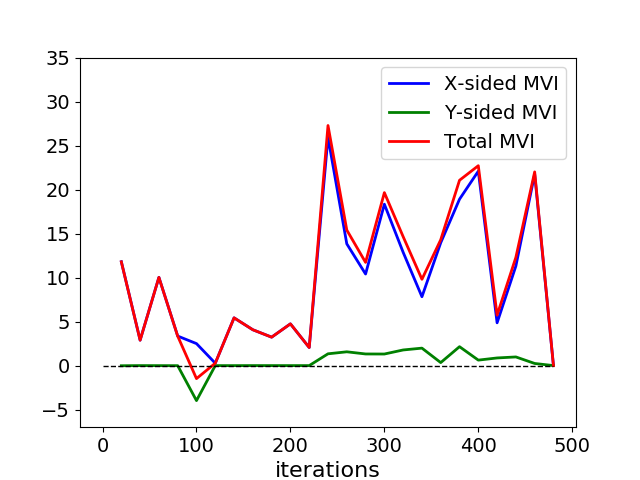
Figure 6: This figure shows the MVI values along the DCGAN’s training trajectory. As we can see, the blue curve stays above $x$ axis in the experiment while the red curve does not.

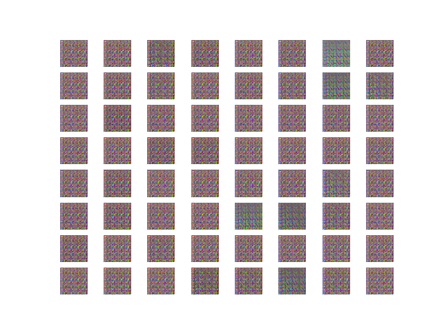
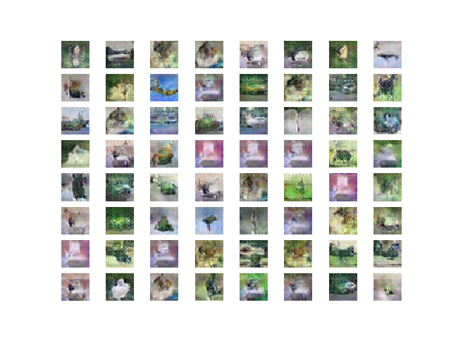
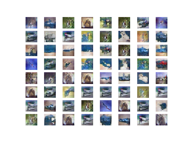
(a) AMSGrad-EG

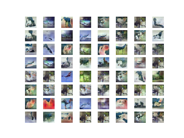
(b) AMSGrad-EG-DRD

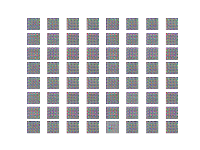
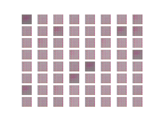
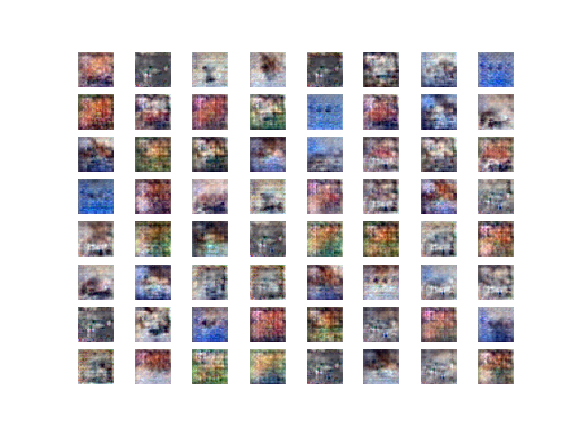
(c) SGDA

Figure 7: These are the generated CIFAR10 figures by the three algorithms after 50, 100, 200 iterations.

Appendix D Stochastic Extra-Gradient and Adaptive Extra-Gradient Algorithms

In a previous paper [LMR⁺20], the authors propose the Optimistic Gradient (OG) method and Optimistic AdaGrad (OAdagrad) method. In this section, we extend them to the Extra-Gradient type algorithms: Stochastic Extra-Gradient (SEG) and Adaptive Extra-Gradient (AEG). We put the result in the appendix because it is just a by-product of this research and not our main result.

Before we introduce our newly-proposed Adaptive Extra-Gradient method, we slightly modify the Stochastic Extra-Gradient (SEG) algorithm, by using different batch sizes in each iteration, as Algorithm 3 below.

Algorithm 3 Stochastic Extra-Gradient (SEG) with batch size

Input: The initial state $\hat{z}_{0}=z_{0}=0$, a constant learning rate $\eta$, a Stochastic First-order Oracle (SFO) $V(z;\xi)$, a sequence of batch sizes $\{m_{k}\}_{k\geqslant 1}$.
 Output: $z_{t}$, $t$ is uniformly chosen from $\{0,1,2,\ldots,N-1\}$.

1:  for $k=1,\ldots,N$ do

2:     (Gradient Evaluation) $g_{k-1}=\frac{1}{m_{k}}\sum_{i=1}^{m_{k}}V(z_{k-1};\xi_{k-1}^{i})$.

3:     (Shadow Update) $\hat{z}_{k}=\Pi_{\mathcal{Z}}[z_{k-1}+\eta\cdot g_{k-1}]$.

4:     (Gradient Evaluation) $\hat{g}_{k-1}=\frac{1}{m_{k}}\sum_{i=1}^{m_{k}}V(\hat{z}_{k};\hat{\xi}_{k-1}^{i})$

5:     (Real Update) $z_{k}=\Pi_{\mathcal{Z}}[z_{k-1}+\eta\cdot\hat{g}_{k-1}]$

6:  end for

Algorithm 4 is a basic idea on the design of AEG algorithm. Here, we use constant batch size $m$ and let $g_{k-1}=\frac{1}{m}\sum_{i=1}^{m}V(z_{k-1},\xi_{k-1}^{i}),\hat{g}_{k-1}=\frac{1}{m}\sum_{i=1}^{m}V(\hat{z}_{k},\hat{\xi}_{k-1}^{i})$ be the estimated gradients on $z_{k-1}$ and $\hat{z}_{k}$ in the $k$-th iteration. Also, $\hat{g}_{1:k}$ is the concatenation of $\hat{g}_{1},\ldots,\hat{g}_{k}$, and $\hat{g}_{1:k,i}$ is its $i$-th row vector. Similarly, $g_{0:k}$ is the concatenation of $g_{0},\ldots,g_{k}$, and $g_{0:k,i}$ is its $i$-th row vector. Note that all the matrices $H_{k},S_{k}$ are diagonal so they don’t require extra computation complexity.

Algorithm 4 Adaptive Extra-Gradient (AEG)

Input: The initial state $\hat{z}_{0}=z_{0}=0,H_{0}=\hat{H}_{0}=\delta I$, a constant learning rate $\eta$, a Stochastic First-order Oracle (SFO) $V(z;\xi)$, a constant batch size $m$.
 Output: $z_{t}$, $t$ is uniformly chosen from $\{0,1,2,\ldots,N-1\}$.

1:  for $k=1,\ldots,N$ do

2:     (Gradient Evaluation) $g_{k-1}=\frac{1}{m}\sum_{i=1}^{m}V(z_{k-1};\xi_{k-1}^{i})$.

3:     (Gradient Concatenation and Norm Calculation) Update $g_{0:k}=[g_{0:k-2}~{}g_{k-1}],s_{k-1,i}=\|\left(g_{0:k-1,i}~{}\hat{g}_{1:k-1,i}\right)\|_{2}~{}~{}i=1,2,\ldots,d$ and $H_{k-1}=\delta I+\mathrm{diag}(s_{k-1})$.

4:     (Shadow Update) $\hat{z}_{k}=z_{k-1}+\eta\cdot H_{k-1}^{-1}g_{k-1}$

5:     (Gradient Evaluation) $\hat{g}_{k-1}=\frac{1}{m}\sum_{i=1}^{m}V(\hat{z}_{k};\hat{\xi}_{k-1}^{i})$.

6:     (Gradient Concatenation and Norm Calculation) Update $\hat{g}_{1:k}=[\hat{g}_{1:k-1}~{}\hat{g}_{k}],\hat{s}_{k-1,i}=\|\left(g_{0:k-1,i}~{}\hat{g}_{1:k,i}\right)\|_{2}~{}~{}i=1,2,\ldots,d$ and $S_{k-1}=\delta I+\mathrm{diag}(\hat{s}_{k-1})$.

7:     (Real Update) $z_{k}=z_{k-1}+\eta\cdot S_{k-1}^{-1}\hat{g}_{k-1}$

8:  end for

Now, we introduce the following two theorems (Theorem D.1 and Theorem D.2), which compare the convergence rates of SEG and its adaptive variant AEG.

Theorem D.1 (Convergence of SEG).

There is an algorithm (Stochastic Extra-Gradient), which given:

• A Stochastic First-order Oracle (SFO) access to the objective function $\phi(x,y):\mathcal{X}\times\mathcal{Y}\rightarrow\mathbb{R}$ where $\mathcal{X}\subseteq\mathbb{R}^{n_{1}},\mathcal{Y}\subseteq\mathbb{R}^{n_{2}}$, which is denoted as: $V(z;\xi)$ and it satisfies the following conditions:

  $$\mathbb{E}[V(z;\xi)]=V(z):=(-\nabla_{x}\phi,\nabla_{y}\phi)\text{~{}~{}and~{}~{}}\mathbb{E}\|V(z;\xi)-V(z)\|^{2}\leqslant\sigma^{2}.$$

  Here, $z:=(x,y)$ and $\mathcal{Z}:=\mathcal{X}\times\mathcal{Y}$. Also: the corresponding MVI function of $-V$ has a solution $z^{*}\in\mathcal{Z}$, which means $\langle-V(z),z-z^{*}\rangle\geqslant 0$ holds for $\forall z\in\mathcal{Z}$.

• A positive real $L$ such that $V$ is $L$-Lipschitz continuous with respect to $\|\cdot\|_{2}$.

• The learning rate $\eta$.

• An initial point $z_{0}\in\mathcal{Z}$.

• The iteration number $N$.

• The sequence of batch sizes in each iteration $\{m_{k}\}_{k\geqslant 1}$.

Then, we output a result $z\in\mathcal{Z}$ which satisfies:

$$\mathbb{E}[r_{\eta}^{2}(z)]\leqslant\frac{4\|z_{0}-z^{*}\|^{2}}{N}+\frac{50\eta^{2}}{N}\sum_{k=0}^{N-1}\frac{\sigma^{2}}{m_{k}}$$

where $r_{\alpha}(z):=\|z-\Pi_{\mathcal{Z}}(z+\alpha\cdot V(z))\|_{2}$ and $\eta\leqslant\frac{1}{4L}$. If $\mathcal{Z}=\mathbb{R}^{n_{1}+n_{2}}$, then the projection operator $\Pi$ is the identity, and $r_{\alpha}(z):=\alpha\cdot\|V(z)\|_{2}$. The inequality above becomes:

$$\mathbb{E}\|V(z)\|_{2}^{2}\leqslant\frac{4\|z_{0}-z^{*}\|^{2}}{\eta^{2}N}+\frac{50}{N}\sum_{k=0}^{N-1}\frac{\sigma^{2}}{m_{k}}.$$

Compared with Optimistic Stochastic Gradient (OSG) method proposed in [LMR⁺20], we can have a larger learning rate in this theorem.

Remark.

Let $\eta=\frac{1}{4L}$. If the batch sizes are constant, which means $m_{k}=m$ for $\forall k$. In order to guarantee that $\mathbb{E}\|V(z)\|^{2}\leqslant\varepsilon^{2}$, we have to make $m=O(1/\varepsilon^{2})$ and $N=O(L^{2}/\varepsilon^{2})$, and the total complexity is $\sum_{k=1}^{N}m_{k}=mN=O(L^{2}/\varepsilon^{4})$. In another scenario where $m_{k}=k+1$ is an increasing sequence, in order to guarantee that $\mathbb{E}\|V(z)\|^{2}\leqslant\varepsilon^{2}$, we have to make $N=O(L^{2}/\varepsilon^{2})$ and then the total complexity is $\sum_{k=1}^{N}m_{k}=\sum_{k=1}^{N}(k+1)=O(L^{4}/\varepsilon^{4})$.

Theorem D.2 (Convergence of AEG).

When our objective function $\phi(x,y)$ satisfies Assumption 1 and 2, as well as the bounded cumulative gradient condition, there exists an algorithm (AEG), given:

• A Stochastic First-order Oracle (SFO) access to the objective function $\phi(x,y):\mathbb{R}^{n_{1}+n_{2}}\rightarrow\mathbb{R}$, which is denoted as: $V(z;\xi)$ and it satisfies the following conditions:

  $$\mathbb{E}[V(z;\xi)]=V(z):=(-\nabla_{x}\phi,\nabla_{y}\phi)\text{~{}~{}and~{}~{}}\mathbb{E}\|V(z;\xi)-V(z)\|^{2}\leqslant\sigma^{2}.$$

  Here, $z:=(x,y)$ and $\mathcal{Z}:=\mathbb{R}^{n_{1}+n_{2}}=\mathbb{R}^{d}$ where $d:=n_{1}+n_{2}$. Also: the corresponding MVI function of $V$ has a solution $z^{*}\in\mathcal{Z}$.

• Positive real numbers $G$, such that $\|V(z;\xi)\|_{2}\leqslant G$ almost surely holds.

• A positive real $L$ such that $V$ is $L$-Lipschitz continuous with respect to $\|\cdot\|_{2}$.

• A universal constant $D>0$ such that $\|z_{k}-z^{*}\|_{2}\leqslant D$ and for all the points on the trajectory of our algorithm.

• An initial point $z_{0}\in\mathcal{Z}$.

• The iteration number $N$.

• A constant batch size $m$.

• A constant $0\leqslant\alpha\leqslant 1/2$ such that: the cumulative gradients are bounded as: $\|(g_{1:k,i}~{}\hat{g}_{1:k,i})\|_{2}\leqslant 2\delta\cdot k^{\alpha}$ for all $i,k$.

• The constant learning rate $\eta\leqslant\frac{\delta}{4L}$.

The output results $z_{0},z_{1},\ldots,z_{N-1}$ satisfies the following inequality:

$$\frac{1}{N}\mathbb{E}\sum_{k=0}^{N-1}\|V(z_{k})\|_{H_{k}^{-1}}^{2}\leqslant\frac{16dD^{2}\delta/\eta^{2}+200d\delta+40dG^{2}/\delta}{N^{1-\alpha}}+\frac{50\delta\sigma^{2}/m+2G^{2}d/\delta}{N}.$$

If we switch the assumption of MVI condition (Assumption 2) to the one-sided MVI condition (Assumption 3), we can slightly modify the Adaptive Extra-Gradient (AEG) method to Adaptive Extra-Gradient with Dual Rate Decay (AEG-DRD), where the learning rate of $\{y_{k}\}$ variables set as $\frac{\eta}{k}$. In the Algorithm 5 below, $H_{k}=\mathrm{Diag}(A_{k},B_{k})$ and $S_{k}=\mathrm{Diag}(C_{k},D_{k})$ where for each $k\in\mathbb{N}$, $A_{k},C_{k}\in\mathbb{R}^{n_{1}\times n_{1}}$ and $B_{k},D_{k}\in\mathbb{R}^{n_{2}\times n_{2}}$. Also, $g_{k}=(g_{k}^{x},g_{k}^{y})$ and $\hat{g}_{k}=(\hat{g}_{k}^{x},\hat{g}_{k}^{y})$ where $g_{k}^{x},\hat{g}_{k}^{x}\in\mathbb{R}^{n_{1}}$ and $g_{k}^{y},\hat{g}_{k}^{y}\in\mathbb{R}^{n_{2}}$.

Algorithm 5 Adaptive Extra-Gradient with Dual Rate Decay (AEG-DRD)

Input: The initial state $\hat{z}_{0}=z_{0}=0,H_{0}=\hat{H}_{0}=\delta I$, a constant learning rate $\eta$, a Stochastic First-order Oracle (SFO) $V(z;\xi)$, a constant batch size $m$.
 Output: $z_{t}$ where $t$ is uniformly chosen from $\{0,1,2,\ldots,N-1\}$.

1:  for $k=1,\ldots,N$ do

2:     (Gradient Evaluation) $g_{k-1}=\frac{1}{m}\sum_{i=1}^{m}V(z_{k-1};\xi_{k-1}^{i})$.

3:     (Gradient Concatenation and Norm Calculation) Update $g_{0:k}=[g_{0:k-2}~{}g_{k-1}],s_{k-1,i}=\|\left(g_{0:k-1,i}~{}\hat{g}_{1:k-1,i}\right)\|_{2}~{}~{}i=1,2,\ldots,d$ and $H_{k-1}=\delta I+\mathrm{diag}(s_{k-1})$.

4:     (Shadow Update of $x$) $\hat{x}_{k}=x_{k-1}+\eta\cdot A_{k-1}^{-1}g_{k-1}^{x}$.

5:     (Shadow Update of $y$) $\hat{y}_{k}=y_{k-1}+\frac{\eta}{k}\cdot B_{k-1}^{-1}g_{k-1}^{y}$.

6:     (Gradient Evaluation) $\hat{g}_{k-1}=\frac{1}{m}\sum_{i=1}^{m}V(\hat{z}_{k};\hat{\xi}_{k-1}^{i})$.

7:     (Gradient Concatenation and Norm Calculation) Update $\hat{g}_{1:k}=[\hat{g}_{1:k-1}~{}\hat{g}_{k}],\hat{s}_{k-1,i}=\|\left(g_{0:k-1,i}~{}\hat{g}_{1:k,i}\right)\|_{2}~{}~{}i=1,2,\ldots,d$ and $S_{k-1}=\delta I+\mathrm{diag}(\hat{s}_{k-1})$.

8:     (Real Update of $x$) $x_{k}=x_{k-1}+\eta\cdot C_{k-1}^{-1}\hat{g}_{k-1}^{x}$.

9:     (Real Update of $y$) $y_{k}=y_{k-1}+\frac{\eta}{k}\cdot D_{k-1}^{-1}\hat{g}_{k-1}^{y}$.

10:  end for

Theorem D.3 (Convergence of AEG-DRD).

When our objective function $\phi(x,y)$ satisfies Assumption 2 and 3, as well as the bounded cumulative gradient condition, there exists an algorithm (AEG-DRD), given:

• A Stochastic First-order Oracle (SFO) access to the objective function $\phi(x,y):\mathbb{R}^{n_{1}+n_{2}}\rightarrow\mathbb{R}$, which is denoted as: $V(z;\xi)$ and it satisfies the following conditions:

  $$\mathbb{E}[V(z;\xi)]=V(z):=(-\nabla_{x}\phi,\nabla_{y}\phi)\text{~{}~{}and~{}~{}}\mathbb{E}\|V(z;\xi)-V(z)\|^{2}\leqslant\sigma^{2}.$$

  Here, $z:=(x,y)$ and $\mathcal{Z}:=\mathbb{R}^{n_{1}+n_{2}}=\mathbb{R}^{d}$ where $d:=n_{1}+n_{2}$. Also: the one-sided MVI function of $V$ has a solution $z^{*}\in\mathcal{Z}$.

• Positive real numbers $G$, such that $\|V(z;\xi)\|_{2}\leqslant G$ almost surely holds.

• A positive real $L$ such that $V$ is $L$-Lipschitz continuous with respect to $\|\cdot\|_{2}$.

• A universal constant $D>0$ such that $\|z_{k}-z^{*}\|_{2}\leqslant D$ and for all the points on the trajectory of our algorithm.

• An initial point $z_{0}\in\mathcal{Z}$.

• The iteration number $N$.

• A constant batch size $m$.

• A constant $0\leqslant\alpha\leqslant 1/2$ such that: the cumulative gradients are bounded as: $\|(g_{1:k,i}~{}\hat{g}_{1:k,i})\|_{2}\leqslant 2\delta\cdot k^{\alpha}$ for all $i,k$.

• The constant learning rate $\eta\leqslant\frac{\delta}{4L}$.

The output results $z_{0},z_{1},\ldots,z_{N-1}$ satisfy the following inequality:

$$\frac{1}{N}\mathbb{E}\sum_{k=1}^{N}\|V_{x}(z_{k-1})\|_{C_{k-1}^{-1}}^{2}\leqslant\frac{16dD^{2}\delta/\eta^{2}+200d\delta+40dG^{2}/\delta}{N^{1-\alpha}}+\frac{24dG^{2}/\delta+50\delta\sigma^{2}/m}{N}.$$

D.1 Proof of Theorem D.1

We recall that in the $t$-th iteration of Stochastic Extra-Gradient (SEG) algorithm with batch size, we have the following updates:

$$\hat{z}_{t} =\Pi_{\mathcal{Z}}\left[z_{t-1}+\eta\cdot\frac{1}{m_{t}}\sum_{i=1}^{m_{t}}V(z_{t-1};\xi_{t-1}^{i})\right]:=\Pi_{\mathcal{Z}}\left[z_{t-1}+\eta\cdot g_{t-1}\right]$$

$$z_{t} =\Pi_{\mathcal{Z}}\left[z_{t-1}+\eta\cdot\frac{1}{m_{t}}\sum_{i=1}^{m_{t}}V(\hat{z}_{t};\hat{\xi}_{t-1}^{i})\right]:=\Pi_{\mathcal{Z}}\left[z_{t-1}+\eta\cdot\hat{g}_{t-1}\right]$$

Before we start our proof, we introduce two simple properties of the projection operation $\Pi_{\mathcal{Z}}$ as follows, where $\mathcal{Z}\subseteq\mathbb{R}^{d}$ is closed and convex.

Lemma D.1.

(1) $\|x-\Pi_{\mathcal{Z}}(x)\|^{2}+\|\Pi_{\mathcal{Z}}(x)-z\|^{2}\geqslant\|x-z\|^{2}$ and $\langle\Pi_{\mathcal{Z}}(x)-x,\Pi_{\mathcal{Z}}(x)-z\rangle\leqslant 0$ holds for $\forall x\in\mathbb{R}^{d},z\in\mathcal{Z}$. Actually, the first inequality is a simple extension of the second one.
(2) The projection operator $\Pi_{\mathcal{Z}}$ is a compression, which means for $\forall x,y\in\mathbb{R}^{d}$, it holds that:

$$\|\Pi_{\mathcal{Z}}(x)-\Pi_{\mathcal{Z}}(y)\|_{2}\leqslant\|x-y\|_{2}.$$

Now, we can start our formal proof.

Lemma D.2.

$$\|z_{k}-z^{*}\|^{2}\leqslant ~{}\|z_{k-1}-z^{*}\|^{2}-(1-6\eta^{2}L^{2})\cdot\|z_{k-1}-\hat{z}_{k}\|^{2}-\|z_{k}-\hat{z}_{k}\|^{2}$$

$$+6\eta^{2}(\|\varepsilon_{k-1}\|^{2}+\|\hat{\varepsilon}_{k-1}\|^{2})+2\langle\hat{z}_{k}-z^{*},\eta\cdot\hat{\varepsilon}_{k-1}\rangle.$$

Here, $\varepsilon_{k-1}=\frac{1}{m_{k}}\sum_{i=1}^{m_{k}}V(z_{k-1};\xi_{k-1}^{i})-V(z_{k-1})$ and $\hat{\varepsilon}_{k-1}=\frac{1}{m_{k}}\sum_{i=1}^{m_{k}}V(\hat{z}_{k};\hat{\xi}_{k}^{i})-V(\hat{z}_{k})$.

Proof of Lemma D.2.

According to the Property (1) of Lemma D.1, we know that:

$$\|z_{k}-z^{*}\|^{2} =\|\Pi_{\mathcal{Z}}[z_{k-1}+\eta\cdot\hat{g}_{k-1}]-z^{*}\|^{2}\leqslant\|z_{k-1}+\eta\cdot\hat{g}_{k-1}-z^{*}\|^{2}-\|z_{k-1}+\eta\cdot\hat{g}_{k-1}-z_{k}\|^{2}$$

$$=\|z_{k-1}-z^{*}\|^{2}-\|z_{k-1}-z_{k}\|^{2}+2\langle\eta\cdot\hat{g}_{k-1},z_{k}-z^{*}\rangle$$

$$=\|z_{k-1}-z^{*}\|^{2}-\|z_{k-1}-\hat{z}_{k}+\hat{z}_{k}-z_{k}\|^{2}+2\langle\eta\cdot\hat{g}_{k-1},\hat{z}_{k}-z^{*}\rangle+2\langle\eta\cdot\hat{g}_{k-1},z_{k}-\hat{z}_{k}\rangle$$

$$=\|z_{k-1}-z^{*}\|^{2}-\|z_{k-1}-\hat{z}_{k}\|^{2}-\|\hat{z}_{k}-z_{k}\|^{2}-2\langle z_{k-1}-\hat{z}_{k},\hat{z}_{k}-z_{k}\rangle$$

$$~{}~{}~{}~{}+2\langle\eta\cdot(V(\hat{z}_{k})+\hat{\varepsilon}_{k-1}),\hat{z}_{k}-z^{*}\rangle+2\langle\eta\cdot\hat{g}_{k-1},z_{k}-\hat{z}_{k}\rangle$$

$$=\|z_{k-1}-z^{*}\|^{2}-\|z_{k-1}-\hat{z}_{k}\|^{2}-\|\hat{z}_{k}-z_{k}\|^{2}+2\langle\hat{z}_{k}-z_{k},\hat{z}_{k}-z_{k-1}-\eta\cdot\hat{g}_{k-1}\rangle$$

$$~{}~{}~{}~{}+2\langle\eta\cdot V(\hat{z}_{k}),\hat{z}_{k}-z^{*}\rangle+2\langle\eta\cdot\hat{\varepsilon}_{k-1},\hat{z}_{k}-z^{*}\rangle$$

Since $z^{*}$ is a solution of MVI inequality, we know that for $\forall z\in\mathcal{Z}$, it holds that $\langle V(z),z-z^{*}\rangle\leqslant 0$,. Therefore:

$$\langle V(\hat{z}_{k}),\hat{z}_{k}-z^{*}\rangle\leqslant 0.$$

Also, since $\hat{z}_{k}=\Pi_{\mathcal{Z}}[z_{k-1}+\eta\cdot g_{k-1}]$, according to the property (1) of Lemma D.1, we have:

$$\langle\hat{z}_{k}-z_{k},\hat{z}_{k}-(z_{k-1}+\eta\cdot g_{k-1})\rangle\leqslant 0.$$

After combining all the three inequalities above, we have:

$$\|z_{k}-z^{*}\|^{2} \leqslant\|z_{k-1}-z^{*}\|^{2}-\|z_{k-1}-\hat{z}_{k}\|^{2}-\|\hat{z}_{k}-z_{k}\|^{2}+2\langle\eta\cdot\hat{\varepsilon}_{k-1},\hat{z}_{k}-z^{*}\rangle$$ (14)

$$~{}~{}~{}~{}+2\langle\hat{z}_{k}-z_{k},\hat{z}_{k}-z_{k-1}-\eta\cdot g_{k-1}+\eta\cdot g_{k-1}-\eta\cdot\hat{g}_{k-1}\rangle$$

$$\leqslant\|z_{k-1}-z^{*}\|^{2}-\|z_{k-1}-\hat{z}_{k}\|^{2}-\|\hat{z}_{k}-z_{k}\|^{2}+2\langle\eta\cdot\hat{\varepsilon}_{k-1},\hat{z}_{k}-z^{*}\rangle$$

$$~{}~{}~{}~{}+2\langle\hat{z}_{k}-z_{k},\eta\cdot g_{k-1}-\eta\cdot\hat{g}_{k-1}\rangle$$

$$\overset{(a)}{\leqslant}\|z_{k-1}-z^{*}\|^{2}-\|z_{k-1}-\hat{z}_{k}\|^{2}-\|\hat{z}_{k}-z_{k}\|^{2}+2\eta\|\hat{z}_{k}-z_{k}\|\cdot\|g_{k-1}-\hat{g}_{k-1}\|$$

$$~{}~{}~{}~{}+2\langle\eta\cdot\hat{\varepsilon}_{k-1},\hat{z}_{k}-z^{*}\rangle$$

$$\overset{(b)}{\leqslant}\|z_{k-1}-z^{*}\|^{2}-\|z_{k-1}-\hat{z}_{k}\|^{2}-\|\hat{z}_{k}-z_{k}\|^{2}+2\eta^{2}\|g_{k-1}-\hat{g}_{k-1}\|^{2}$$

$$~{}~{}~{}~{}+2\langle\eta\cdot\hat{\varepsilon}_{k-1},\hat{z}_{k}-z^{*}\rangle$$

Here, $(a)$ holds by Cauchy-Schwarz inequality, and $(b)$ holds because by using the property (2) of Lemma D.1, we know that

$$\|\hat{z}_{k}-z_{k}\| =\|\Pi_{\mathcal{Z}}[z_{k-1}+\eta\cdot g_{k-1}]-\Pi_{\mathcal{Z}}[z_{k-1}+\eta\cdot\hat{g}_{k-1}]\|\leqslant\|(z_{k-1}+\eta\cdot g_{k-1})-(z_{k-1}+\eta\cdot\hat{g}_{k-1})\|$$

$$=\eta\cdot\|g_{k-1}-\hat{g}_{k-1}\|.$$

Now, we focus on dealing with $\|g_{k-1}-\hat{g}_{k-1}\|$. In fact:

$$\|g_{k-1}-\hat{g}_{k-1}\|^{2} \overset{(c)}{=}\|V(z_{k-1})-V(\hat{z}_{k})+\varepsilon_{k-1}-\hat{\varepsilon}_{k-1}\|^{2}$$ (15)

$$\overset{(d)}{\leqslant}3\left(\|V(z_{k-1})-V(\hat{z}_{k})\|^{2}+\|\varepsilon_{k-1}\|^{2}+\|\hat{\varepsilon}_{k-1}\|^{2}\right)$$

$$\overset{(e)}{\leqslant}3L^{2}\|z_{k-1}-\hat{z}_{k}\|^{2}+3(\|\varepsilon_{k-1}\|^{2}+\|\hat{\varepsilon}_{k-1}\|^{2})$$

Here, $(c)$ holds by the definition of $\varepsilon_{k-1},\hat{\varepsilon}_{k-1}$. $(d)$ holds because by Cauchy Inequality, $\|x+y+z\|^{2}\leqslant 3(\|x\|^{2}+\|y\|^{2}+\|z\|^{2})$ always holds. $(e)$ holds because we’ve assumed that $V(z)$ is $L$-Lipschitz continuous under $\|\cdot\|_{2}$ norm. Combine Equation (14) and (15), we obtain that:

$$\|z_{k}-z^{*}\|^{2} \leqslant\|z_{k-1}-z^{*}\|^{2}-(1-6\eta^{2}L^{2})\|z_{k-1}-\hat{z}_{k}\|^{2}-\|\hat{z}_{k}-z_{k}\|^{2}+6\eta^{2}\cdot(\|\varepsilon_{k-1}\|^{2}+\|\hat{\varepsilon}_{k-1}\|^{2})$$

$$~{}~{}~{}~{}+2\langle\eta\cdot\hat{\varepsilon}_{k-1},\hat{z}_{k}-z^{*}\rangle,$$

which is exactly what we want to prove in this lemma. ∎

Now, we come back to our Theorem D.1. Notice that

$$r_{\eta}(z_{k})^{2} =\|z_{k}-\Pi_{\mathcal{Z}}[z_{k}+\eta\cdot V(z_{k})]\|^{2}=\|z_{k}-\hat{z}_{k+1}+\hat{z}_{k+1}-\Pi_{\mathcal{Z}}[z_{k}+\eta\cdot V(z_{k})]\|^{2}$$ (16)

$$\overset{(a)}{\leqslant}2\left(\|z_{k}-\hat{z}_{k+1}\|^{2}+\|\hat{z}_{k+1}-\Pi_{\mathcal{Z}}[z_{k}+\eta\cdot V(z_{k})]\|^{2}\right)$$

$$=2\left(\|z_{k}-\hat{z}_{k+1}\|^{2}+\left\|\Pi_{\mathcal{Z}}[z_{k}+\eta\cdot g_{k}]-\Pi_{\mathcal{Z}}[z_{k}+\eta\cdot V(z_{k})]\right\|^{2}\right)$$

$$\overset{(b)}{\leqslant}2\|z_{k}-\hat{z}_{k+1}\|^{2}+2\eta^{2}\cdot\|\varepsilon_{k}\|^{2}$$

Here, $(a)$ comes from Cauchy Inequality and $(b)$ holds because of the property (2) of Lemma D.1.

Proof of Theorem D.1.

Put $k=1,2,\ldots,N$ in Lemma D.2 and add them up, and we obtain that:

$$\|z_{N}-z^{*}\|^{2} \leqslant\|z_{0}-z^{*}\|^{2}-(1-6\eta^{2}L^{2})\cdot\sum_{k=0}^{N-1}\|z_{k}-\hat{z}_{k+1}\|^{2}-\sum_{k=1}^{N}\|z_{k}-\hat{z}_{k}\|^{2}$$

$$~{}~{}~{}~{}+6\eta^{2}\cdot\sum_{k=0}^{N-1}\left(\|\varepsilon_{k}\|^{2}+\|\hat{\varepsilon}_{k}\|^{2}\right)+2\sum_{k=1}^{N}\langle\hat{z}_{k}-z^{*},\eta\cdot\hat{\varepsilon}_{k-1}\rangle.$$

Therefore, after combining with Equation (16), we have:

$$\sum_{k=0}^{N-1}r_{\eta}(z_{k})^{2} \leqslant 2\sum_{k=0}^{N-1}\|z_{k}-\hat{z}_{k+1}\|^{2}+2\eta^{2}\cdot\sum_{k=0}^{N-1}\|\varepsilon_{k}\|^{2}$$

$$\leqslant\frac{2}{1-6\eta^{2}L^{2}}\left(\|z_{0}-z^{*}\|^{2}+6\eta^{2}\cdot\sum_{k=0}^{N-1}\left(\|\varepsilon_{k}\|^{2}+\|\hat{\varepsilon}_{k}\|^{2}\right)+2\sum_{k=1}^{N}\langle\hat{z}_{k}-z^{*},\eta\cdot\hat{\varepsilon}_{k-1}\rangle\right)$$

$$~{}~{}~{}~{}+2\eta^{2}\cdot\sum_{k=0}^{N-1}\|\varepsilon_{k}\|^{2}$$

Since $\eta\leqslant\frac{1}{4L}$, we have $1-6\eta^{2}L^{2}\geqslant\frac{1}{2}$. After taking expectation on the inequality above, it holds that:

$$\frac{1}{N}\sum_{k=0}^{N-1}\mathbb{E}[r_{\eta}(z_{k})^{2}] \leqslant\frac{4\|z_{0}-z^{*}\|^{2}}{N}+\frac{48\eta^{2}}{N}\sum_{k=0}^{N-1}\frac{\sigma^{2}}{m_{k}}+\frac{2\eta^{2}}{N}\sum_{k=0}^{N-1}\frac{\sigma^{2}}{m_{k}}$$

$$=\frac{4\|z_{0}-z^{*}\|^{2}}{N}+\frac{50\eta^{2}}{N}\sum_{k=0}^{N-1}\frac{\sigma^{2}}{m_{k}}$$

which comes to our conclusion. Here, we use the fact that $\mathbb{E}\|\varepsilon_{k}\|^{2}\leqslant\frac{\sigma^{2}}{m_{k}},\mathbb{E}\|\hat{\varepsilon}_{k}\|^{2}\leqslant\frac{\sigma^{2}}{m_{k}}$ and $\mathbb{E}\langle\hat{z}_{k}-z^{*},\eta\cdot\hat{\varepsilon}_{k-1}\rangle=0$. ∎

D.2 Proof of Theorem D.2

We recall that in the $t$-th iteration of Adaptive Extra-Gradient, our update is as follows:

$$\hat{z}_{t} =z_{t-1}+\eta\cdot H_{t-1}^{-1}g_{t-1}$$

$$z_{t} =z_{t-1}+\eta\cdot S_{t-1}^{-1}\hat{g}_{t}.$$

Now we begin our proof by introducing several lemmas.

Lemma D.3.

$$\|z_{k}-z^{*}\|_{s_{k-1}}^{2}\leqslant\|z_{k-1}-z^{*}\|_{s_{k-1}}^{2}-\|z_{k-1}-\hat{z}_{k}\|_{s_{k-1}}^{2}+\|z_{k}-\hat{z}_{k}\|_{s_{k-1}}^{2}+2\langle\eta\cdot\hat{\varepsilon}_{k},\hat{z}_{k}-z^{*}\rangle.$$

Here, $\hat{\varepsilon}_{k}=\hat{g}_{k}-V(\hat{z}_{k})=\frac{1}{m}\sum_{i=1}^{m}V(\hat{z}_{k};\hat{\xi}_{i})-V(\hat{z}_{k})$.

Proof of Lemma D.3.

According to our update rule, we know that:

$$\|z_{k}-z^{*}\|_{S_{k-1}}^{2} =\|z_{k-1}+\eta\cdot S_{k-1}^{-1}\hat{g}_{k}-z^{*}\|_{S_{k-1}}^{2}$$

$$=\|z_{k-1}+\eta\cdot S_{k-1}^{-1}\hat{g}_{k}-z^{*}\|_{S_{k-1}}^{2}-\|z_{k-1}+\eta\cdot S_{k-1}^{-1}\hat{g}_{k}-z_{k}\|_{S_{k-1}}^{2}$$

$$=\|z_{k-1}-z^{*}\|_{S_{k-1}}^{2}-\|z_{k-1}-z_{k}\|_{S_{k-1}}^{2}+2\langle\eta\cdot\hat{g}_{k},z_{k}-z^{*}\rangle$$

$$=\|z_{k-1}-z^{*}\|_{S_{k-1}}^{2}-\|z_{k-1}-\hat{z}_{k}+\hat{z}_{k}-z_{k}\|_{S_{k-1}}^{2}+2\langle\eta\cdot\hat{g}_{k},z_{k}-\hat{z}_{k}\rangle+2\langle\eta\cdot\hat{g}_{k},\hat{z}_{k}-z^{*}\rangle$$

$$=\|z_{k-1}-z^{*}\|_{S_{k-1}}^{2}-\|z_{k-1}-\hat{z}_{k}\|_{S_{k-1}}^{2}-\|\hat{z}_{k}-z_{k}\|_{S_{k-1}}^{2}-2\langle S_{k-1}(z_{k-1}-\hat{z}_{k}),\hat{z}_{k}-z_{k}\rangle$$

$$~{}~{}~{}~{}+2\langle\eta\cdot\hat{g}_{k},z_{k}-\hat{z}_{k}\rangle+2\langle\eta\cdot\hat{g}_{k},\hat{z}_{k}-z^{*}\rangle$$

$$=\|z_{k-1}-z^{*}\|_{S_{k-1}}^{2}-\|z_{k-1}-\hat{z}_{k}\|_{S_{k-1}}^{2}-\|\hat{z}_{k}-z_{k}\|_{S_{k-1}}^{2}+2\langle\eta\cdot\hat{g}_{k},\hat{z}_{k}-z^{*}\rangle$$

$$~{}~{}~{}~{}+2\langle z_{k}-\hat{z}_{k},S_{k-1}(z_{k-1}-\hat{z}_{k}+\eta\cdot S_{k-1}^{-1}\hat{g}_{k})\rangle$$

$$=\|z_{k-1}-z^{*}\|_{S_{k-1}}^{2}-\|z_{k-1}-\hat{z}_{k}\|_{S_{k-1}}^{2}-\|\hat{z}_{k}-z_{k}\|_{S_{k-1}}^{2}+2\langle\eta\cdot\hat{g}_{k},\hat{z}_{k}-z^{*}\rangle$$

$$~{}~{}~{}~{}+2\langle z_{k}-\hat{z}_{k},S_{k-1}(z_{k}-\hat{z}_{k})\rangle$$

$$=\|z_{k-1}-z^{*}\|_{S_{k-1}}^{2}-\|z_{k-1}-\hat{z}_{k}\|_{S_{k-1}}^{2}+\|\hat{z}_{k}-z_{k}\|_{S_{k-1}}^{2}+2\langle\eta\cdot\hat{g}_{k},\hat{z}_{k}-z^{*}\rangle$$

Notice that $\hat{g}_{k}=V(\hat{z}_{k})+\hat{\varepsilon}_{k}$. Since $z^{*}$ is a solution of MVI which means $\langle V(z),z-z^{*}\rangle\leqslant 0$ holds for $\forall z\in\mathcal{Z}$, so $\langle V(\hat{z}_{k}),\hat{z}_{k}-z^{*}\rangle\leqslant 0$. Therefore:

$$\langle\eta\cdot\hat{g}_{k},\hat{z}_{k}-z^{*}\rangle=\langle\eta\cdot(V(\hat{z}_{k})+\hat{\varepsilon}_{k}),\hat{z}_{k}-z^{*}\rangle\leqslant\langle\eta\cdot\hat{\varepsilon}_{k},\hat{z}_{k}-z^{*}\rangle.$$

Combine it with the inequality above, we obtain that:

$$\|z_{k}-z^{*}\|_{S_{k-1}}^{2}\leqslant\|z_{k-1}-z^{*}\|_{S_{k-1}}^{2}-\|z_{k-1}-\hat{z}_{k}\|_{S_{k-1}}^{2}+\|\hat{z}_{k}-z_{k}\|_{S_{k-1}}^{2}+2\langle\eta\cdot\hat{\varepsilon}_{k},\hat{z}_{k}-z^{*}\rangle,$$

which comes to our conclusion. ∎

In the lemma above, it’s worth mentioned that the expectation of $\langle\eta\cdot\hat{\varepsilon}_{k},\hat{z}_{k}-z^{*}\rangle$ is 0. In the next lemma, we are going to deal with the upper bound of $\|\hat{z}_{k}-z_{k}\|_{S_{k-1}}^{2}$. Before that, we notice the following fact:

$$H_{0}\preceq S_{0}\preceq H_{1}\preceq S_{1}\preceq\ldots\preceq H_{N}\preceq S_{N}.$$

Lemma D.4.

$$\|z_{k}-\hat{z}_{k}\|_{S_{k-1}}^{2} \leqslant\frac{6\eta^{2}L^{2}}{\delta^{2}}\|z_{k-1}-\hat{z}_{k}\|_{S_{k-1}}^{2}+6\eta^{2}\left(\|\varepsilon_{k-1}\|_{H_{k-1}^{-1}}^{2}+\|\hat{\varepsilon}_{k-1}\|_{S_{k-1}^{-1}}^{2}\right)$$

$$~{}~{}~{}~{}+2\eta^{2}\cdot\|(S_{k-1}^{-1}-H_{k-1}^{-1})g_{k-1}\|_{S_{k-1}}^{2}$$

Proof of Lemma D.4.

Since $\hat{z}_{k}=z_{k-1}+\eta\cdot H_{k-1}^{-1}g_{k-1}$ and $z_{k}=z_{k-1}+\eta\cdot S_{k-1}^{-1}\hat{g}_{k}$, we have:

$$\|z_{k}-\hat{z}_{k}\|_{S_{k-1}}^{2} =\eta^{2}\cdot\|S_{k-1}^{-1}\hat{g}_{k}-H_{k-1}^{-1}g_{k-1}\|_{S_{k-1}}^{2}=\eta^{2}\cdot\|S_{k-1}^{-1}\hat{g}_{k}-S_{k-1}^{-1}g_{k-1}+S_{k-1}^{-1}g_{k-1}-H_{k-1}^{-1}g_{k-1}\|_{S_{k-1}}^{2}$$

$$\overset{(a)}{\leqslant}2\eta^{2}\cdot\left(\|S_{k-1}^{-1}(\hat{g}_{k}-g_{k-1})\|_{S_{k-1}}^{2}+\|(S_{k-1}^{-1}-H_{k-1}^{-1})g_{k-1}\|_{S_{k-1}}^{2}\right)$$

$$=2\eta^{2}\cdot\left(\|\hat{g}_{k}-g_{k-1}\|_{S_{k-1}^{-1}}^{2}+\|(S_{k-1}^{-1}-H_{k-1}^{-1})g_{k-1}\|_{S_{k-1}}^{2}\right)$$

$$=2\eta^{2}\cdot\|V(\hat{z}_{k})-V(z_{k-1})+\hat{\varepsilon}_{k-1}-\varepsilon_{k-1}\|_{S_{k-1}^{-1}}^{2}+2\eta^{2}\cdot\|(S_{k-1}^{-1}-H_{k-1}^{-1})g_{k-1}\|_{S_{k-1}}^{2}$$

$$\overset{(b)}{\leqslant}6\eta^{2}\cdot\left(\|V(\hat{z}_{k})-V(z_{k-1})\|_{S_{k-1}^{-1}}^{2}+\|\hat{\varepsilon}_{k-1}\|_{S_{k-1}^{-1}}^{2}+\|\varepsilon_{k-1}\|_{S_{k-1}^{-1}}^{2}\right)$$

$$~{}~{}~{}~{}+2\eta^{2}\cdot\|(S_{k-1}^{-1}-H_{k-1}^{-1})g_{k-1}\|_{S_{k-1}}^{2}$$

$$\overset{(c)}{\leqslant}6\eta^{2}\cdot\left(\frac{L^{2}}{\delta^{2}}\|\hat{z}_{k}-z_{k-1}\|_{S_{k-1}}^{2}+\|\hat{\varepsilon}_{k-1}\|_{S_{k-1}^{-1}}^{2}+\|\varepsilon_{k-1}\|_{H_{k-1}^{-1}}^{2}\right)$$

$$~{}~{}~{}~{}+2\eta^{2}\cdot\|(S_{k-1}^{-1}-H_{k-1}^{-1})g_{k-1}\|_{S_{k-1}}^{2},$$

which comes to our conclusion. Here, $(a)$ holds since for any norm $\|\cdot\|_{A}$, we have $\|x+y\|_{A}^{2}\leqslant(\|x\|_{A}+\|y\|_{A})^{2}\leqslant 2(\|x\|_{A}^{2}+\|y\|_{A}^{2})$, and $(b)$ holds for the similar reason. $(c)$ holds because of the following two reasons:
(1) Since $V$ is $L$-Lipschitz continuous, and $\delta I\preceq S_{k-1}$, we have:

$$\|V(\hat{z}_{k})-V(z_{k-1})\|_{S_{k-1}^{-1}}^{2}\leqslant\frac{1}{\delta}\|V(\hat{z}_{k})-V(z_{k-1})\|_{2}^{2}\leqslant\frac{L^{2}}{\delta}\|\hat{z}_{k}-z_{k-1}\|^{2}\leqslant\frac{L^{2}}{\delta^{2}}\|\hat{z}_{k}-z_{k-1}\|_{S_{k-1}}^{2}.$$

(2) Since $H_{k-1}\preceq S_{k-1}$, we have $S_{k-1}^{-1}\preceq H_{k-1}^{-1}$. Therefore,

$$\|\varepsilon_{k-1}\|_{S_{k-1}^{-1}}^{2}\leqslant\|\varepsilon_{k-1}\|_{H_{k-1}^{-1}}^{2}.$$

∎

Since $\eta\leqslant\frac{\delta}{4L}$, then $\frac{6\eta^{2}L^{2}}{\delta^{2}}\leqslant\frac{1}{2}$. According to Lemma D.3 and Lemma D.4, we have:

$$\|z_{k}-z^{*}\|_{S_{k-1}}^{2} \leqslant\|z_{k-1}-z^{*}\|_{S_{k-1}}^{2}-\|z_{k-1}-\hat{z}_{k}\|_{S_{k-1}}^{2}+2\langle\eta\cdot\hat{\varepsilon}_{k-1},\hat{z}_{k}-z^{*}\rangle+\frac{1}{2}\|z_{k-1}-\hat{z}_{k}\|_{S_{k-1}}^{2}$$

$$~{}~{}~{}~{}+6\eta^{2}\left(\|\varepsilon_{k-1}\|_{H_{k-1}^{-1}}^{2}+\|\hat{\varepsilon}_{k-1}\|_{S_{k-1}^{-1}}^{2}\right)+2\eta^{2}\cdot\|(S_{k-1}^{-1}-H_{k-1}^{-1})g_{k-1}\|_{S_{k-1}}^{2}$$

which means:

$$\frac{1}{2}\|z_{k-1}-\hat{z}_{k}\|_{S_{k-1}}^{2} \leqslant\|z_{k-1}-z^{*}\|_{S_{k-1}}^{2}-\|z_{k}-z^{*}\|_{S_{k-1}}^{2}+2\langle\eta\cdot\hat{\varepsilon}_{k-1},\hat{z}_{k}-z^{*}\rangle$$ (17)

$$~{}~{}~{}~{}+6\eta^{2}\left(\|\varepsilon_{k-1}\|_{H_{k-1}^{-1}}^{2}+\|\hat{\varepsilon}_{k-1}\|_{S_{k-1}^{-1}}^{2}\right)+2\eta^{2}\cdot\|(S_{k-1}^{-1}-H_{k-1}^{-1})g_{k-1}\|_{S_{k-1}}^{2}$$

Notice that, $\|z_{k-1}-\hat{z}_{k}\|_{S_{k-1}}^{2}=\|\eta\cdot H_{k-1}^{-1}g_{k-1}\|_{S_{k-1}}^{2}$. Therefore,

$$\|g_{k-1}\|_{S_{k-1}^{-1}}^{2} =\|S_{k-1}^{-1}g_{k-1}\|_{S_{k-1}}^{2}=\|H_{k-1}^{-1}g_{k-1}+(S_{k-1}^{-1}-H_{k-1}^{-1})g_{k-1}\|_{S_{k-1}}^{2}$$ (18)

$$\leqslant 2\left(\|H_{k-1}^{-1}g_{k-1}\|_{S_{k-1}}^{2}+\|(S_{k-1}^{-1}-H_{k-1}^{-1})g_{k-1}\|_{S_{k-1}}^{2}\right)$$

$$=\frac{2}{\eta^{2}}\cdot\|z_{k-1}-\hat{z}_{k}\|_{S_{k-1}}^{2}+2\cdot\|(S_{k-1}^{-1}-H_{k-1}^{-1})g_{k-1}\|_{S_{k-1}}^{2}$$

Combine Equation (17) and (18), we obtain that:

$$\|g_{k-1}\|_{S_{k-1}^{-1}}^{2} \leqslant\frac{4}{\eta^{2}}\cdot(\|z_{k-1}-z^{*}\|_{S_{k-1}}^{2}-\|z_{k}-z^{*}\|_{S_{k-1}}^{2})+\frac{8}{\eta}\langle\hat{\varepsilon}_{k-1},\hat{z}_{k}-z^{*}\rangle$$ (19)

$$~{}~{}~{}~{}+24\cdot\left(\|\varepsilon_{k-1}\|_{H_{k-1}^{-1}}^{2}+\|\hat{\varepsilon}_{k-1}\|_{S_{k-1}^{-1}}^{2}\right)+10\cdot\|(S_{k-1}^{-1}-H_{k-1}^{-1})g_{k-1}\|_{S_{k-1}}^{2}$$

In the inequality above, the expectation of $\langle\hat{\varepsilon}_{k-1},\hat{z}_{k}-z^{*}\rangle$ is 0, which can be ignored under expectation. Since we are going to do the summation over $k=1,2,\ldots,N$ in the future, in the following lemmas, we analyze the upper bounds of $\sum_{k=1}^{N}(\|z_{k-1}-z^{*}\|_{S_{k-1}}^{2}-\|z_{k}-z^{*}\|_{S_{k-1}}^{2})$, $\sum_{k=1}^{N}\|(S_{k-1}^{-1}-H_{k-1}^{-1})g_{k-1}\|_{S_{k-1}}^{2}$, and $\sum_{k=1}^{N}(\|\varepsilon_{k-1}\|_{H_{k-1}^{-1}}^{2}+\|\hat{\varepsilon}_{k-1}\|_{S_{k-1}^{-1}}^{2})$

Lemma D.5.

$$\sum_{k=1}^{N}\left(\|z_{k-1}-z^{*}\|_{S_{k-1}}^{2}-\|z_{k}-z^{*}\|_{S_{k-1}}^{2}\right)\leqslant 2dD^{2}\delta\cdot N^{\alpha}.$$

Proof of Lemma D.5.

Notice that

$$~{}~{}\sum_{k=1}^{N}\left(\|z_{k-1}-z^{*}\|_{S_{k-1}}^{2}-\|z_{k}-z^{*}\|_{S_{k-1}}^{2}\right)\leqslant\|z_{0}-z^{*}\|_{S_{0}}^{2}+\sum_{k=1}^{N-1}\left(\|z_{k}-z^{*}\|_{S_{k}}^{2}-\|z_{k}-z^{*}\|_{S_{k-1}}^{2}\right)$$

$$=\|z_{0}-z^{*}\|_{S_{0}}^{2}+\sum_{k=1}^{N-1}\left[(z_{k}-z^{*})^{\top}(S_{k}-S_{k-1})\cdot(z_{k}-z^{*})\right]$$

$$\leqslant D^{2}\cdot\mathrm{tr}(S_{0})+\sum_{k=1}^{N-1}D^{2}\cdot(\mathrm{tr}(S_{k})-\mathrm{tr}(S_{k-1}))=D^{2}\cdot\mathrm{tr}(S_{N-1})<D^{2}\cdot 2d\delta N^{\alpha},$$

which comes to our conclusion. ∎

Lemma D.6.

$$\sum_{k=1}^{N}\|(S_{k-1}^{-1}-H_{k-1}^{-1})g_{k-1}\|_{S_{k-1}}^{2}\leqslant\frac{2dG^{2}\cdot N^{\alpha}}{\delta}.$$

Proof of Lemma D.6.

For any $\delta\leqslant x<y$, we notice that:

$$y\left(\frac{1}{x}-\frac{1}{y}\right)^{2}=\frac{(y-x)^{2}}{x^{2}y}<\frac{y-x}{x^{2}}\leqslant\frac{y-x}{\delta^{2}}.$$ (20)

Therefore, we have:

$$~{}~{}\sum_{k=1}^{N}\|(S_{k-1}^{-1}-H_{k-1}^{-1})g_{k-1}\|_{S_{k-1}}^{2}\leqslant\sum_{k=1}^{N}g_{k-1}^{\top}(H_{k-1}^{-1}-S_{k-1}^{-1})S_{k-1}(H_{k-1}^{-1}-S_{k-1}^{-1})g_{k-1}$$

$$\leqslant\sum_{k=1}^{N}G^{2}\cdot\mathrm{tr}\left((H_{k-1}^{-1}-S_{k-1}^{-1})S_{k-1}(H_{k-1}^{-1}-S_{k-1}^{-1})\right)$$

$$\overset{(a)}{\leqslant}\sum_{k=1}^{N}\frac{G^{2}}{\delta^{2}}\cdot[\mathrm{tr}(S_{k-1})-\mathrm{tr}(H_{k-1})]$$

$$\leqslant\frac{G^{2}}{\delta^{2}}\cdot\mathrm{tr}(S_{N-1})<\frac{G^{2}}{\delta^{2}}\cdot 2d\delta\cdot N^{\alpha}=\frac{2dG^{2}\cdot N^{\alpha}}{\delta}.$$

Here, $(a)$ holds because of Equation (20). ∎

Lemma D.7.

$$\mathbb{E}\sum_{k=1}^{N}\left(\|\varepsilon_{k-1}\|_{H_{k-1}^{-1}}^{2}+\|\hat{\varepsilon}_{k-1}\|_{S_{k-1}^{-1}}^{2}\right)\leqslant\frac{\delta\sigma^{2}}{m}+4d\delta\cdot N^{\alpha}.$$

The proof of this lemma can be found in [DHS11]. Combine Lemma D.5, D.6, D.7 with Equation (19), we obtain that:

$$\mathbb{E}\sum_{k=1}^{N}\|g_{k-1}\|_{S_{k-1}^{-1}}^{2}\leqslant\frac{4}{\eta^{2}}\cdot 2dD^{2}\delta N^{\alpha}+24\cdot\left(\frac{\delta\sigma^{2}}{m}+4d\delta\cdot N^{\alpha}\right)+10\cdot\frac{2dG^{2}\cdot N^{\alpha}}{\delta}.$$

Now, we replace the $g_{k-1}$ with the true gradient $V(z_{k-1})$ as follows:

$$~{}~{}~{}\mathbb{E}\sum_{k=1}^{N}\|V(z_{k-1})\|_{H_{k-1}^{-1}}^{2}=\mathbb{E}\sum_{k=1}^{N}\|g_{k-1}+\varepsilon_{k-1}\|_{H_{k-1}^{-1}}^{2}\leqslant 2\cdot\mathbb{E}\sum_{k=1}^{N}\|g_{k-1}\|_{H_{k-1}^{-1}}^{2}+2\cdot\mathbb{E}\sum_{k=1}^{N}\|\varepsilon_{k-1}\|_{H_{k-1}^{-1}}^{2}$$

$$\overset{(a)}{\leqslant}2\cdot\mathbb{E}\sum_{k=1}^{N}\left[\|g_{k-1}\|_{S_{k-1}^{-1}}^{2}+g_{k-1}^{\top}(H_{k-1}^{-1}-S_{k-1}^{-1})\cdot g_{k-1}\right]+2\cdot\left(\frac{\delta\sigma^{2}}{m}+4d\delta\cdot N^{\alpha}\right)$$

$$\leqslant 2\cdot\mathbb{E}\sum_{k=1}^{N}\|g_{k-1}\|_{S_{k-1}^{-1}}^{2}+2\cdot\left(\frac{\delta\sigma^{2}}{m}+4d\delta\cdot N^{\alpha}\right)+2G^{2}\cdot\sum_{k=1}^{N}\left[\mathrm{tr}(H_{k-1}^{-1})-\mathrm{tr}(S_{k-1}^{-1})\right]$$

$$\leqslant\frac{8}{\eta^{2}}\cdot 2dD^{2}\delta N^{\alpha}+50\cdot\left(\frac{\delta\sigma^{2}}{m}+4d\delta\cdot N^{\alpha}\right)+20\cdot\frac{2dG^{2}\cdot N^{\alpha}}{\delta}+2G^{2}\cdot\mathrm{tr}(H_{0}^{-1})$$

$$=\frac{8}{\eta^{2}}\cdot 2dD^{2}\delta N^{\alpha}+50\cdot\left(\frac{\delta\sigma^{2}}{m}+4d\delta\cdot N^{\alpha}\right)+20\cdot\frac{2dG^{2}\cdot N^{\alpha}}{\delta}+\frac{2G^{2}d}{\delta}.$$

Here, $(a)$ uses the conclusion of Lemma D.7. Finally, we multiplies $\frac{1}{N}$ on both sides and finish the proof:

$$\frac{1}{N}\mathbb{E}\sum_{k=0}^{N-1}\|V(z_{k})\|_{H_{k}^{-1}}^{2}\leqslant\frac{16dD^{2}\delta/\eta^{2}+200d\delta+40dG^{2}/\delta}{N^{1-\alpha}}+\frac{50\delta\sigma^{2}/m+2G^{2}d/\delta}{N}.$$

D.3 Proof of Theorem D.3

In this proof, we are still using the Adaptive Extra-Gradient (AEG) algorithm, which its $t$-th iteration is:

$$\hat{z}_{t} =z_{t-1}+\eta\cdot H_{t-1}^{-1}g_{t-1}$$

$$z_{t} =z_{t-1}+\eta\cdot S_{t-1}^{-1}\hat{g}_{t}.$$

For simplicity, we split the update of $x$ variable and $y$ variable. Recall that $H_{k}=\mathrm{Diag}(A_{k},B_{k})$ and $S_{k}=\mathrm{Diag}(C_{k},D_{k})$ where for each $k\in\mathbb{N}$, $A_{k},C_{k}\in\mathbb{R}^{n_{1}\times n_{1}}$ and $B_{k},D_{k}\in\mathbb{R}^{n_{2}\times n_{2}}$. Also, we denote $g_{k}=(g_{k}^{x},g_{k}^{y})$ and $\hat{g}_{k}=(\hat{g}_{k}^{x},\hat{g}_{k}^{y})$ where $g_{k}^{x},\hat{g}_{k}^{x}\in\mathbb{R}^{n_{1}}$ and $g_{k}^{y},\hat{g}_{k}^{y}\in\mathbb{R}^{n_{2}}$. Then, the update above can be rewritten as:

$$\hat{x}_{t} =x_{t-1}+\eta\cdot A_{t-1}^{-1}g_{t-1}^{x}$$

$$\hat{y}_{t} =y_{t-1}+\frac{\eta}{t}\cdot B_{t-1}^{-1}g_{t-1}^{y}$$

$$x_{t} =x_{t-1}+\eta\cdot C_{t-1}^{-1}\hat{g}_{t}^{x}$$

$$y_{t} =y_{t-1}+\frac{\eta}{t}\cdot D_{t-1}^{-1}\hat{g}_{t}^{y}.$$

Similar to Lemma D.3, we only focus on the $x$-s, and then we can get our upper bound for $\|x_{k}-x^{*}\|_{C_{k-1}}^{2}$, which is the first step of our proof.

Lemma D.8.

$$\|x_{k}-x^{*}\|_{C_{k-1}}^{2}\leqslant\|x_{k-1}-x^{*}\|_{C_{k-1}}^{2}-\|x_{k-1}-\hat{x}_{k}\|_{C_{k-1}}^{2}+\|x_{k}-\hat{x}_{k}\|_{C_{k-1}}^{2}+2\langle\eta\cdot\hat{\varepsilon}_{k-1}^{x},\hat{x}_{k}-x^{*}\rangle.$$

Proof of Lemma D.8.

According to the update rule of $x_{k},\hat{x}_{k}$, we know that:

$$\|x_{k}-x^{*}\|_{C_{k-1}}^{2} =\|x_{k-1}+\eta\cdot C_{k-1}^{-1}\hat{g}_{k}^{x}-x^{*}\|_{C_{k-1}}^{2}$$

$$=\|x_{k-1}+\eta\cdot C_{k-1}^{-1}\hat{g}_{k}^{x}-x^{*}\|_{C_{k-1}}^{2}-\|x_{k-1}+\eta\cdot C_{k-1}^{-1}\hat{g}_{k}^{x}-x_{k}\|_{C_{k-1}}^{2}$$

$$=\|x_{k-1}-x^{*}\|_{C_{k-1}}^{2}-\|x_{k-1}-x_{k}\|_{C_{k-1}}^{2}+2\langle\eta\cdot\hat{g}_{k}^{x},x_{k}-x^{*}\rangle$$

$$=\|x_{k-1}-x^{*}\|_{C_{k-1}}^{2}-\|x_{k-1}-\hat{x}_{k}+\hat{x}_{k}-x_{k}\|_{C_{k-1}}^{2}+2\langle\eta\cdot\hat{g}_{k}^{x},x_{k}-\hat{x}_{k}\rangle+2\langle\eta\cdot\hat{g}_{k}^{x},\hat{x}_{k}-x^{*}\rangle$$

$$=\|x_{k-1}-x^{*}\|_{C_{k-1}}^{2}-\|x_{k-1}-\hat{x}_{k}\|_{C_{k-1}}^{2}-\|\hat{x}_{k}-x_{k}\|_{C_{k-1}}^{2}-2\langle C_{k-1}(x_{k-1}-\hat{x}_{k}),\hat{x}_{k}-x_{k}\rangle$$

$$~{}~{}~{}~{}+2\langle\eta\cdot\hat{g}_{k}^{x},x_{k}-\hat{x}_{k}\rangle+2\langle\eta\cdot\hat{g}_{k}^{x},\hat{x}_{k}-x^{*}\rangle$$

$$=\|x_{k-1}-x^{*}\|_{C_{k-1}}^{2}-\|x_{k-1}-\hat{x}_{k}\|_{C_{k-1}}^{2}-\|\hat{x}_{k}-x_{k}\|_{C_{k-1}}^{2}+2\langle\eta\cdot\hat{g}_{k}^{x},\hat{x}_{k}-x^{*}\rangle$$

$$~{}~{}~{}~{}+2\langle x_{k}-\hat{x}_{k},C_{k-1}(x_{k-1}-\hat{x}_{k}+\eta\cdot C_{k-1}^{-1}\hat{g}_{k}^{x})\rangle$$

$$=\|x_{k-1}-x^{*}\|_{C_{k-1}}^{2}-\|x_{k-1}-\hat{x}_{k}\|_{C_{k-1}}^{2}-\|\hat{x}_{k}-x_{k}\|_{C_{k-1}}^{2}+2\langle\eta\cdot\hat{g}_{k}^{x},\hat{x}_{k}-x^{*}\rangle$$

$$~{}~{}~{}~{}+2\langle x_{k}-\hat{x}_{k},C_{k-1}(x_{k}-\hat{x}_{k})\rangle$$

$$=\|x_{k-1}-x^{*}\|_{C_{k-1}}^{2}-\|x_{k-1}-\hat{x}_{k}\|_{C_{k-1}}^{2}+\|\hat{x}_{k}-x_{k}\|_{C_{k-1}}^{2}+2\langle\eta\cdot\hat{g}_{k}^{x},\hat{x}_{k}-x^{*}\rangle$$

Notice that $\hat{g}_{k}=V(\hat{z}_{k})+\hat{\varepsilon}_{k-1}\Rightarrow\hat{g}_{k}^{x}=V_{x}(\hat{z}_{k})+\hat{\varepsilon}_{k-1}^{x}$. Since $z^{*}$ satisfies the one-side MVI condition, therefore $\langle V_{x}(z),x-x^{*}\rangle\leqslant 0$ holds for $\forall z=(x,y)\in\mathcal{Z}$, so $\langle V_{x}(\hat{z}_{k}),\hat{x}_{k}-x^{*}\rangle\leqslant 0$. Therefore:

$$\langle\eta\cdot\hat{g}_{k}^{x},\hat{x}_{k}-x^{*}\rangle=\langle\eta\cdot(V_{x}(\hat{z}_{k})+\hat{\varepsilon}_{k-1}^{x}),\hat{x}_{k}-x^{*}\rangle\leqslant\langle\eta\cdot\hat{\varepsilon}_{k-1}^{x},\hat{x}_{k}-x^{*}\rangle.$$

Combine it with the inequality above, we obtain that:

$$\|x_{k}-x^{*}\|_{C_{k-1}}^{2}\leqslant\|x_{k-1}-x^{*}\|_{C_{k-1}}^{2}-\|x_{k-1}-\hat{x}_{k}\|_{C_{k-1}}^{2}+\|\hat{x}_{k}-x_{k}\|_{C_{k-1}}^{2}+2\langle\eta\cdot\hat{\varepsilon}_{k-1}^{x},\hat{x}_{k}-x^{*}\rangle,$$

which comes to our conclusion. ∎

Notice that the term $2\langle\eta\cdot\hat{\varepsilon}_{k-1}^{x},\hat{x}_{k}-x^{*}\rangle$ has zero mean, which can be ignored when taking expectation. In the next step, we upper bound the $\|\hat{x}_{k}-x_{k}\|_{C_{k-1}}^{2}$ term. Also, we notice the following facts:

$$A_{0}\preceq C_{0}\preceq A_{1}\preceq C_{1}\preceq\ldots\preceq A_{N}\preceq C_{N},$$

$$B_{0}\preceq D_{0}\preceq B_{1}\preceq D_{1}\preceq\ldots\preceq B_{N}\preceq D_{N}.$$

Lemma D.9.

$$\|x_{k}-\hat{x}_{k}\|_{C_{k-1}}^{2} \leqslant\frac{6\eta^{2}L^{2}}{\delta^{2}}\left(\|x_{k-1}-\hat{x}_{k}\|_{C_{k-1}}^{2}+\|y_{k-1}-\hat{y}_{k}\|_{D_{k-1}}^{2}\right)+6\eta^{2}\left(\|\varepsilon_{k-1}\|_{H_{k-1}^{-1}}^{2}+\|\hat{\varepsilon}_{k-1}\|_{S_{k-1}^{-1}}^{2}\right)$$

$$~{}~{}~{}~{}+2\eta^{2}\cdot\|(C_{k-1}^{-1}-A_{k-1}^{-1})g_{k-1}^{x}\|_{C_{k-1}}^{2}$$

Proof of Lemma D.9.

Since $\hat{x}_{k}=x_{k-1}+\eta\cdot A_{k-1}^{-1}g_{k-1}^{x}$ and $x_{k}=x_{k-1}+\eta\cdot C_{k-1}^{-1}\hat{g}_{k}^{x}$, we have:

$$\|x_{k}-\hat{x}_{k}\|_{C_{k-1}}^{2} =\eta^{2}\cdot\|C_{k-1}^{-1}\hat{g}_{k}^{x}-A_{k-1}^{-1}g_{k-1}^{x}\|_{C_{k-1}}^{2}=\eta^{2}\cdot\|C_{k-1}^{-1}\hat{g}_{k}^{x}-C_{k-1}^{-1}g_{k-1}^{x}+C_{k-1}^{-1}g_{k-1}^{x}-A_{k-1}^{-1}g_{k-1}^{x}\|_{C_{k-1}}^{2}$$

$$\overset{(a)}{\leqslant}2\eta^{2}\cdot\left(\|C_{k-1}^{-1}(\hat{g}_{k}^{x}-g_{k-1}^{x})\|_{C_{k-1}}^{2}+\|(C_{k-1}^{-1}-A_{k-1}^{-1})g_{k-1}^{x}\|_{C_{k-1}}^{2}\right)$$

$$=2\eta^{2}\cdot\left(\|\hat{g}_{k}^{x}-g_{k-1}^{x}\|_{C_{k-1}^{-1}}^{2}+\|(C_{k-1}^{-1}-A_{k-1}^{-1})g_{k-1}^{x}\|_{C_{k-1}}^{2}\right)$$

$$\overset{(b)}{\leqslant}2\eta^{2}\cdot\left(\|\hat{g}_{k}-g_{k-1}\|_{S_{k-1}^{-1}}^{2}+\|(C_{k-1}^{-1}-A_{k-1}^{-1})g_{k-1}^{x}\|_{C_{k-1}}^{2}\right)$$

$$=2\eta^{2}\cdot\|V(\hat{z}_{k})-V(z_{k-1})+\hat{\varepsilon}_{k-1}-\varepsilon_{k-1}\|_{S_{k-1}^{-1}}^{2}+2\eta^{2}\cdot\|(C_{k-1}^{-1}-A_{k-1}^{-1})g_{k-1}^{x}\|_{C_{k-1}}^{2}$$

$$\overset{(c)}{\leqslant}6\eta^{2}\cdot\left(\|V(\hat{z}_{k})-V(z_{k-1})\|_{S_{k-1}^{-1}}^{2}+\|\hat{\varepsilon}_{k-1}\|_{S_{k-1}^{-1}}^{2}+\|\varepsilon_{k-1}\|_{S_{k-1}^{-1}}^{2}\right)$$

$$~{}~{}~{}~{}+2\eta^{2}\cdot\|(C_{k-1}^{-1}-A_{k-1}^{-1})g_{k-1}^{x}\|_{C_{k-1}}^{2}$$

$$\overset{(d)}{\leqslant}6\eta^{2}\cdot\left(\frac{L^{2}}{\delta^{2}}\|\hat{z}_{k}-z_{k-1}\|_{S_{k-1}}^{2}+\|\hat{\varepsilon}_{k-1}\|_{S_{k-1}^{-1}}^{2}+\|\varepsilon_{k-1}\|_{H_{k-1}^{-1}}^{2}\right)$$

$$~{}~{}~{}~{}+2\eta^{2}\cdot\|(C_{k-1}^{-1}-A_{k-1}^{-1})g_{k-1}^{x}\|_{C_{k-1}}^{2}$$

$$\overset{(e)}{=}6\eta^{2}\cdot\left(\frac{L^{2}}{\delta^{2}}\|\hat{x}_{k}-x_{k-1}\|_{C_{k-1}}^{2}+\frac{L^{2}}{\delta^{2}}\|\hat{y}_{k}-y_{k-1}\|_{D_{k-1}}^{2}+\|\hat{\varepsilon}_{k-1}\|_{S_{k-1}^{-1}}^{2}+\|\varepsilon_{k-1}\|_{H_{k-1}^{-1}}^{2}\right)$$

$$~{}~{}~{}~{}+2\eta^{2}\cdot\|(C_{k-1}^{-1}-A_{k-1}^{-1})g_{k-1}^{x}\|_{C_{k-1}}^{2}$$

which comes to our conclusion. Here, $(a)$ holds since for any norm $\|\cdot\|_{A}$, we have $\|x+y\|_{A}^{2}\leqslant(\|x\|_{A}+\|y\|_{A})^{2}\leqslant 2(\|x\|_{A}^{2}+\|y\|_{A}^{2})$, and $(c)$ holds for the similar reason. (b) holds because $\|\hat{g}_{k}-g_{k-1}\|_{S_{k-1}^{-1}}^{2}=\|\hat{g}_{k}^{x}-g_{k-1}^{x}\|_{C_{k-1}^{-1}}^{2}+\|\hat{g}_{k}^{y}-g_{k-1}^{y}\|_{D_{k-1}^{-1}}^{2}\geqslant\|\hat{g}_{k}^{x}-g_{k-1}^{x}\|_{C_{k-1}^{-1}}^{2}$, and (e) holds for the same reason. $(d)$ holds because of the following two reasons:
(1) Since $V$ is $L$-Lipschitz continuous, and $\delta I\preceq S_{k-1}$, we have:

$$\|V(\hat{z}_{k})-V(z_{k-1})\|_{S_{k-1}^{-1}}^{2}\leqslant\frac{1}{\delta}\|V(\hat{z}_{k})-V(z_{k-1})\|_{2}^{2}\leqslant\frac{L^{2}}{\delta}\|\hat{z}_{k}-z_{k-1}\|^{2}\leqslant\frac{L^{2}}{\delta^{2}}\|\hat{z}_{k}-z_{k-1}\|_{S_{k-1}}^{2}.$$

(2) Since $H_{k-1}\preceq S_{k-1}$, we have $S_{k-1}^{-1}\preceq H_{k-1}^{-1}$. Therefore,

$$\|\varepsilon_{k-1}\|_{S_{k-1}^{-1}}^{2}\leqslant\|\varepsilon_{k-1}\|_{H_{k-1}^{-1}}^{2}.$$

∎

Since we require our learning rate $\eta\leqslant\frac{\delta}{4L}$, the coefficient above $\frac{6\eta^{2}L^{2}}{\delta^{2}}<\frac{1}{2}$. After combining Lemma D.8 and Lemma D.9, we obtain that:

$$\|x_{k}-x^{*}\|_{C_{k-1}}^{2} \leqslant\|x_{k-1}-x^{*}\|_{C_{k-1}}^{2}-\frac{1}{2}\|x_{k-1}-\hat{x}_{k}\|_{C_{k-1}}^{2}+\frac{1}{2}\|y_{k-1}-\hat{y}_{k}\|_{D_{k-1}}^{2}+2\langle\eta\cdot\hat{\varepsilon}_{k-1}^{x},\hat{x}_{k}-x^{*}\rangle$$ (21)

$$~{}~{}~{}~{}+6\eta^{2}\left(\|\varepsilon_{k-1}\|_{H_{k-1}^{-1}}^{2}+\|\hat{\varepsilon}_{k-1}\|_{S_{k-1}^{-1}}^{2}\right)+2\eta^{2}\cdot\|(C_{k-1}^{-1}-A_{k-1}^{-1})g_{k-1}^{x}\|_{C_{k-1}}^{2},$$

which means:

$$\frac{1}{2}\|x_{k-1}-\hat{x}_{k}\|_{C_{k-1}}^{2} \leqslant\|x_{k-1}-x^{*}\|_{C_{k-1}}^{2}-\|x_{k}-x^{*}\|_{C_{k-1}}^{2}+\frac{1}{2}\|y_{k-1}-\hat{y}_{k}\|_{D_{k-1}}^{2}+2\langle\eta\cdot\hat{\varepsilon}_{k-1}^{x},\hat{x}_{k}-x^{*}\rangle$$ (22)

$$~{}~{}~{}~{}+6\eta^{2}\left(\|\varepsilon_{k-1}\|_{H_{k-1}^{-1}}^{2}+\|\hat{\varepsilon}_{k-1}\|_{S_{k-1}^{-1}}^{2}\right)+2\eta^{2}\cdot\|(C_{k-1}^{-1}-A_{k-1}^{-1})g_{k-1}^{x}\|_{C_{k-1}}^{2},$$

Notice that, $\|x_{k-1}-\hat{x}_{k}\|_{C_{k-1}}^{2}=\|\eta\cdot A_{k-1}^{-1}g_{k-1}^{x}\|_{C_{k-1}}^{2}$. Therefore,

$$\|g_{k-1}^{x}\|_{C_{k-1}^{-1}}^{2} =\|C_{k-1}^{-1}g_{k-1}^{x}\|_{C_{k-1}}^{2}=\|A_{k-1}^{-1}g_{k-1}^{x}+(C_{k-1}^{-1}-A_{k-1}^{-1})g_{k-1}^{x}\|_{C_{k-1}}^{2}$$ (23)

$$\leqslant 2\left(\|A_{k-1}^{-1}g_{k-1}^{x}\|_{C_{k-1}}^{2}+\|(C_{k-1}^{-1}-A_{k-1}^{-1})g_{k-1}^{x}\|_{C_{k-1}}^{2}\right)$$

$$=\frac{2}{\eta^{2}}\cdot\|x_{k-1}-\hat{x}_{k}\|_{C_{k-1}}^{2}+2\cdot\|(C_{k-1}^{-1}-A_{k-1}^{-1})g_{k-1}^{x}\|_{C_{k-1}}^{2}.$$

Combining Equation (22) and Equation (23), we get:

$$\|g_{k-1}^{x}\|_{C_{k-1}^{-1}}^{2} \leqslant\frac{4}{\eta^{2}}\left(\|x_{k-1}-x^{*}\|_{C_{k-1}}^{2}-\|x_{k}-x^{*}\|_{C_{k-1}}^{2}\right)+\frac{2}{\eta^{2}}\|y_{k-1}-\hat{y}_{k}\|_{D_{k-1}}^{2}+\frac{8}{\eta^{2}}\langle\eta\cdot\hat{\varepsilon}_{k-1}^{x},\hat{x}_{k}-x^{*}\rangle$$ (24)

$$~{}~{}~{}~{}+24\left(\|\varepsilon_{k-1}\|_{H_{k-1}^{-1}}^{2}+\|\hat{\varepsilon}_{k-1}\|_{S_{k-1}^{-1}}^{2}\right)+10\cdot\|(C_{k-1}^{-1}-A_{k-1}^{-1})g_{k-1}^{x}\|_{C_{k-1}}^{2},$$

Then, we take summation over $k=1,2,\ldots,N$ and take expectation, and we can obtain that:

$$\mathbb{E}\sum_{k=1}^{N}\|g_{k-1}^{x}\|_{C_{k-1}^{-1}}^{2} \leqslant\frac{4}{\eta^{2}}\mathbb{E}\sum_{k=1}^{N}\left(\|x_{k-1}-x^{*}\|_{C_{k-1}}^{2}-\|x_{k}-x^{*}\|_{C_{k-1}}^{2}\right)+\frac{2}{\eta^{2}}\mathbb{E}\sum_{k=1}^{N}\|y_{k-1}-\hat{y}_{k}\|_{D_{k-1}}^{2}$$ (25)

$$~{}+24\cdot\mathbb{E}\sum_{k=1}^{N}\left(\|\varepsilon_{k-1}\|_{H_{k-1}^{-1}}^{2}+\|\hat{\varepsilon}_{k-1}\|_{S_{k-1}^{-1}}^{2}\right)+10\cdot\mathbb{E}\sum_{k=1}^{N}\|(C_{k-1}^{-1}-A_{k-1}^{-1})g_{k-1}^{x}\|_{C_{k-1}}^{2}.$$

In the following steps, we will upper bound the four terms above on the right side. The third term $\mathbb{E}\sum_{k=1}^{N}\left(\|\varepsilon_{k-1}\|_{H_{k-1}^{-1}}^{2}+\|\hat{\varepsilon}_{k-1}\|_{S_{k-1}^{-1}}^{2}\right)$ can be upper bounded by using Lemma D.7:

$$\mathbb{E}\sum_{k=1}^{N}\left(\|\varepsilon_{k-1}\|_{H_{k-1}^{-1}}^{2}+\|\hat{\varepsilon}_{k-1}\|_{S_{k-1}^{-1}}^{2}\right)\leqslant\frac{\delta\sigma^{2}}{m}+4d\delta\cdot N^{\alpha}.$$ (26)

The fourth term $\mathbb{E}\sum_{k=1}^{N}\|(C_{k-1}^{-1}-A_{k-1}^{-1})g_{k-1}^{x}\|_{C_{k-1}}^{2}$ can be upper bounded by using Lemma D.6:

$$\mathbb{E}\sum_{k=1}^{N}\|(C_{k-1}^{-1}-A_{k-1}^{-1})g_{k-1}^{x}\|_{C_{k-1}}^{2}\leqslant\mathbb{E}\sum_{k=1}^{N}\|(S_{k-1}^{-1}-H_{k-1}^{-1})g_{k-1}\|_{S_{k-1}}^{2}\leqslant\frac{2dG^{2}\cdot N^{\alpha}}{\delta}.$$

For the first term $\mathbb{E}\sum_{k=1}^{N}\left(\|x_{k-1}-x^{*}\|_{C_{k-1}}^{2}-\|x_{k}-x^{*}\|_{C_{k-1}}^{2}\right)$, we can use the similar techniques as Lemma D.5.

Lemma D.10.

$$\sum_{k=1}^{N}\left(\|x_{k-1}-x^{*}\|_{C_{k-1}}^{2}-\|x_{k}-x^{*}\|_{C_{k-1}}^{2}\right)\leqslant 2dD^{2}\delta\cdot N^{\alpha}.$$

Proof of Lemma D.10.

Notice that

$$~{}~{}\sum_{k=1}^{N}\left(\|x_{k-1}-x^{*}\|_{C_{k-1}}^{2}-\|x_{k}-x^{*}\|_{C_{k-1}}^{2}\right)\leqslant\|x_{0}-x^{*}\|_{C_{0}}^{2}+\sum_{k=1}^{N-1}\left(\|x_{k}-x^{*}\|_{C_{k}}^{2}-\|x_{k}-x^{*}\|_{C_{k-1}}^{2}\right)$$

$$=\|x_{0}-x^{*}\|_{C_{0}}^{2}+\sum_{k=1}^{N-1}\left[(x_{k}-x^{*})^{\top}(C_{k}-C_{k-1})\cdot(x_{k}-x^{*})\right]$$

$$\leqslant D^{2}\cdot\mathrm{tr}(C_{0})+\sum_{k=1}^{N-1}D^{2}\cdot(\mathrm{tr}(C_{k})-\mathrm{tr}(C_{k-1}))=D^{2}\cdot\mathrm{tr}(C_{N-1})<D^{2}\cdot\mathrm{tr}(S_{N-1})\leqslant D^{2}\cdot 2d\delta N^{\alpha},$$

which comes to our conclusion. ∎

For the second term $\mathbb{E}\sum_{k=1}^{N}\|y_{k-1}-\hat{y}_{k}\|_{D_{k-1}}^{2}$, notice that:

$$\sum_{k=1}^{N}\|y_{k-1}-\hat{y}_{k}\|_{D_{k-1}}^{2} =\sum_{k=1}^{N}\frac{\eta^{2}}{k^{2}}\cdot\|B_{k-1}^{-1}g_{k-1}^{y}\|_{D_{k-1}}^{2}=\sum_{k=1}^{N}\frac{\eta^{2}}{k^{2}}\cdot g_{k-1}^{y\top}B_{k-1}^{-1}D_{k-1}B_{k-1}^{-1}g_{k-1}^{y}$$

$$\leqslant\sum_{k=1}^{N}\frac{\eta^{2}}{k^{2}}\cdot G^{2}\mathrm{tr}(B_{k-1}^{-1}D_{k-1}B_{k-1}^{-1})<\sum_{k=1}^{N}\frac{\eta^{2}}{k^{2}}G^{2}\cdot\frac{2d\delta k^{\alpha}}{\delta^{2}}$$

$$=\frac{2\eta^{2}dG^{2}}{\delta}\sum_{k=1}^{N}\frac{1}{k^{2-\alpha}}$$

Here, we notice that:

$$\sum_{k=1}^{N}\frac{1}{k^{2-\alpha}}<1+\int_{1}^{N}\frac{1}{x^{2-\alpha}}dx<1+\int_{1}^{N}\frac{1}{x^{3/2}}dx=1+2\left(1-\frac{1}{\sqrt{N}}\right)<3.$$

Therefore:

$$\sum_{k=1}^{N}\|y_{k-1}-\hat{y}_{k}\|_{D_{k-1}}^{2}<\frac{6\eta^{2}dG^{2}}{\delta}.$$

According to Equation (25):

$$\mathbb{E}\sum_{k=1}^{N}\|g_{k-1}^{x}\|_{C_{k-1}^{-1}}^{2} \leqslant\frac{4}{\eta^{2}}\cdot 2dD^{2}\delta\cdot N^{\alpha}+\frac{2}{\eta^{2}}\cdot\frac{6\eta^{2}dG^{2}}{\delta}+24\cdot\left(\frac{\delta\sigma^{2}}{m}+4d\delta\cdot N^{\alpha}\right)+10\cdot\frac{2dG^{2}\cdot N^{\alpha}}{\delta}$$ (27)

$$=N^{\alpha}\cdot\left(\frac{8dD^{2}\delta}{\eta^{2}}+96d\delta+\frac{20dG^{2}}{\delta}\right)+\frac{12dG^{2}}{\delta}+\frac{24\delta\sigma^{2}}{m}.$$

Finally, we replace the $g_{k-1}^{x}$ above with the actual gradient $V_{x}(z_{k-1})$. Since:

$$\|V_{x}(z_{k-1})\|_{C_{k-1}^{-1}}^{2}\leqslant\left(\|g_{k-1}^{x}\|_{C_{k-1}^{-1}}+\|\varepsilon_{k-1}^{x}\|_{C_{k-1}^{-1}}\right)^{2}\leqslant 2\left(\|g_{k-1}^{x}\|_{C_{k-1}^{-1}}^{2}+\|\varepsilon_{k-1}^{x}\|_{C_{k-1}^{-1}}^{2}\right),$$

we can upper bound the target term $\mathbb{E}\sum_{k=1}^{N}\|V_{x}(z_{k-1})\|_{C_{k-1}^{-1}}^{2}$:

$$\mathbb{E}\sum_{k=1}^{N}\|V_{x}(z_{k-1})\|_{C_{k-1}^{-1}}^{2}\leqslant\mathbb{E}\sum_{k=1}^{N}2\left(\|g_{k-1}^{x}\|_{C_{k-1}^{-1}}^{2}+\|\varepsilon_{k-1}^{x}\|_{C_{k-1}^{-1}}^{2}\right)\leqslant 2\mathbb{E}\sum_{k=1}^{N}\|g_{k-1}^{x}\|_{C_{k-1}^{-1}}^{2}+2\mathbb{E}\sum_{k=1}^{N}\|\varepsilon_{k-1}^{x}\|_{C_{k-1}^{-1}}^{2}$$ (28)

$$~{}~{}~{}~{}\overset{(a)}{\leqslant}N^{\alpha}\cdot\left(\frac{16dD^{2}\delta}{\eta^{2}}+192d\delta+\frac{40dG^{2}}{\delta}\right)+\frac{24dG^{2}}{\delta}+\frac{48\delta\sigma^{2}}{m}+2\mathbb{E}\sum_{k=1}^{N}\left(\|\varepsilon_{k-1}\|_{H_{k-1}^{-1}}^{2}+\|\hat{\varepsilon}_{k-1}\|_{S_{k-1}^{-1}}^{2}\right)$$

$$~{}~{}~{}~{}\overset{(b)}{\leqslant}N^{\alpha}\cdot\left(\frac{16dD^{2}\delta}{\eta^{2}}+192d\delta+\frac{40dG^{2}}{\delta}\right)+\frac{24dG^{2}}{\delta}+\frac{48\delta\sigma^{2}}{m}+2\left(\frac{\delta\sigma^{2}}{m}+4d\delta\cdot N^{\alpha}\right)$$

$$~{}~{}~{}~{}=N^{\alpha}\cdot\left(\frac{16dD^{2}\delta}{\eta^{2}}+200d\delta+\frac{40dG^{2}}{\delta}\right)+\frac{24dG^{2}}{\delta}+\frac{50\delta\sigma^{2}}{m},$$

which means that:

$$\frac{1}{N}\mathbb{E}\sum_{k=1}^{N}\|V_{x}(z_{k-1})\|_{C_{k-1}^{-1}}^{2}\leqslant\frac{16dD^{2}\delta/\eta^{2}+200d\delta+40dG^{2}/\delta}{N^{1-\alpha}}+\frac{24dG^{2}/\delta+50\delta\sigma^{2}/m}{N},$$

which comes to our conclusion.

References

• [ABC+16] Martín Abadi, Paul Barham, Jianmin Chen, Zhifeng Chen, Andy Davis, Jeffrey Dean, Matthieu Devin, Sanjay Ghemawat, Geoffrey Irving, Michael Isard, et al. Tensorflow: A system for large-scale machine learning. In 12th USENIX symposium on operating systems design and implementation (OSDI 16), pages 265–283, 2016.
• [ACB17] Martin Arjovsky, Soumith Chintala, and Léon Bottou. Wasserstein generative adversarial networks. In International conference on machine learning, pages 214–223. PMLR, 2017.
• [AL20] Zeyuan Allen-Zhu and Yuanzhi Li. Feature purification: How adversarial training performs robust deep learning. arXiv preprint arXiv:2005.10190, 2020.
• [AMLG19] Waïss Azizian, Ioannis Mitliagkas, Simon Lacoste-Julien, and Gauthier Gidel. A tight and unified analysis of extragradient for a whole spectrum of differentiable games. arXiv: Learning, 2019.
• [AZL19] Zeyuan Allen-Zhu and Yuanzhi Li. What can resnet learn efficiently, going beyond kernels? arXiv preprint arXiv:1905.10337, 2019.
• [AZL20a] Zeyuan Allen-Zhu and Yuanzhi Li. Backward feature correction: How deep learning performs deep learning. arXiv preprint arXiv:2001.04413, 2020.
• [AZL20b] Zeyuan Allen-Zhu and Yuanzhi Li. Towards understanding ensemble, knowledge distillation and self-distillation in deep learning. arXiv preprint arXiv:2012.09816, 2020.
• [AZL21] Zeyuan Allen-Zhu and Yuanzhi Li. Forward super-resolution: How can gans learn hierarchical generative models for real-world distributions. arXiv preprint arXiv:2106.02619, 2021.
• [BDMU18] Amitabh Basu, Soham De, Anirbit Mukherjee, and Enayat Ullah. Convergence guarantees for rmsprop and adam in non-convex optimization and their comparison to nesterov acceleration on autoencoders. 2018.
• [Cho03] Gobinda G Chowdhury. Natural language processing. Annual review of information science and technology, 37(1):51–89, 2003.
• [CLSH19] Xiangyi Chen, Sijia Liu, Ruoyu Sun, and Mingyi Hong. On the convergence of a class of adam-type algorithms for non-convex optimization. In ICLR 2019 : 7th International Conference on Learning Representations, 2019.
• [Dar83] John Darzentas. Problem complexity and method efficiency in optimization. 1983.
• [DCLT18] Jacob Devlin, Ming-Wei Chang, Kenton Lee, and Kristina N. Toutanova. Bert: Pre-training of deep bidirectional transformers for language understanding. In Proceedings of the 2019 Conference of the North American Chapter of the Association for Computational Linguistics: Human Language Technologies, Volume 1 (Long and Short Papers), pages 4171–4186, 2018.
• [DHS11] John C Duchi, Elad Hazan, and Yoram Singer. Adaptive subgradient methods for online learning and stochastic optimization. Journal of Machine Learning Research, 12:2121–2159, 2011.
• [DISZ18] Constantinos Daskalakis, Andrew Ilyas, Vasilis Syrgkanis, and Haoyang Zeng. Training gans with optimism. In ICLR 2018 : International Conference on Learning Representations 2018, 2018.
• [DL15] Cong D. Dang and Guanghui Lan. On the convergence properties of non-euclidean extragradient methods for variational inequalities with generalized monotone operators. Computational Optimization and Applications, 60(2):277–310, 2015.
• [GBC16] Ian Goodfellow, Yoshua Bengio, and Aaron Courville. Deep Learning. 2016.
• [GBV+19] Gauthier Gidel, Hugo Berard, Gaatan Vignoud, Pascal Vincent, and Simon Lacoste-Julien. A variational inequality perspective on generative adversarial networks. In ICLR 2019 : 7th International Conference on Learning Representations, 2019.
• [GHP+19] Gauthier Gidel, Reyhane Askari Hemmat, Mohammad Pezeshki, Gabriel Huang, Rémi Le Priol, Simon Lacoste-Julien, and Ioannis Mitliagkas. Negative momentum for improved game dynamics. In The 22nd International Conference on Artificial Intelligence and Statistics, pages 1802–1811, 2019.
• [GPM+14] Ian Goodfellow, Jean Pouget-Abadie, Mehdi Mirza, Bing Xu, David Warde-Farley, Sherjil Ozair, Aaron Courville, and Yoshua Bengio. Generative adversarial nets. In Advances in Neural Information Processing Systems 27, pages 2672–2680, 2014.
• [HMC20] Ya-Ping Hsieh, Panayotis Mertikopoulos, and Volkan Cevher. The limits of min-max optimization algorithms: convergence to spurious non-critical sets. arXiv preprint arXiv:2006.09065, 2020.
• [HS66] Philip Hartman and Guido Stampacchia. On some non-linear elliptic differential-functional equations. Acta Mathematica, 115(1):271–310, 1966.
• [IJOT17] Alfredo N. Iusem, Alejandro Jofré, Roberto Imbuzeiro Oliveira, and Philip Thompson. Extragradient method with variance reduction for stochastic variational inequalities. Siam Journal on Optimization, 27(2):686–724, 2017.
• [JNT11] Anatoli Juditsky, Arkadii S. Nemirovski, and Claire Tauvel. Solving variational inequalities with stochastic mirror-prox algorithm. Stochastic Systems, 1(1):17–58, 2011.
• [Joh59] Erik Johnsen. Arrow, hurwicz and uzawa: Studies in linear and non-linear programming, stanford univeristy press 1958. 229 s., 7,50. Ledelse and Erhvervsøkonomi, 23, 1959.
• [KB15] Diederik P. Kingma and Jimmy Lei Ba. Adam: A method for stochastic optimization. In ICLR 2015 : International Conference on Learning Representations 2015, 2015.
• [KLY18] Robert Kleinberg, Yuanzhi Li, and Yang Yuan. An alternative view: When does sgd escape local minima? arXiv preprint arXiv:1802.06175, 2018.
• [Kor76] G. M. Korpelevich. The extragradient method for finding saddle points and other problems. Matecon, 12:747–756, 1976.
• [LBBH98] Yann LeCun, Léon Bottou, Yoshua Bengio, and Patrick Haffner. Gradient-based learning applied to document recognition. Proceedings of the IEEE, 86(11):2278–2324, 1998.
• [LH19] Ilya Loshchilov and Frank Hutter. Decoupled weight decay regularization. In ICLR 2019 : 7th International Conference on Learning Representations, 2019.
• [LLRY18] Qihang Lin, Mingrui Liu, Hassan Rafique, and Tianbao Yang. Solving weakly-convex-weakly-concave saddle-point problems as weakly-monotone variational inequality. 2018.
• [LMR+20] Mingrui Liu, Youssef Mroueh, Jerret Ross, Wei Zhang, Xiaodong Cui, Payel Das, and Tianbao Yang. Towards better understanding of adaptive gradient algorithms in generative adversarial nets. In ICLR 2020 : Eighth International Conference on Learning Representations, 2020.
• [LMZ18] Yuanzhi Li, Tengyu Ma, and Hongyang Zhang. Algorithmic regularization in over-parameterized matrix sensing and neural networks with quadratic activations. In COLT, 2018.
• [LMZ20] Yuanzhi Li, Tengyu Ma, and Hongyang R Zhang. Learning over-parametrized two-layer neural networks beyond ntk. In Conference on Learning Theory, pages 2613–2682, 2020.
• [LO18] Xiaoyu Li and Francesco Orabona. On the convergence of stochastic gradient descent with adaptive stepsizes. In The 22nd International Conference on Artificial Intelligence and Statistics, pages 983–992, 2018.
• [LXLS19] Liangchen Luo, Yuanhao Xiong, Yan Liu, and Xu Sun. Adaptive gradient methods with dynamic bound of learning rate. In ICLR 2019 : 7th International Conference on Learning Representations, 2019.
• [LY17] Yuanzhi Li and Yang Yuan. Convergence analysis of two-layer neural networks with relu activation. In Advances in Neural Information Processing Systems, pages 597–607. http://arxiv.org/abs/1705.09886, 2017.
• [MH17] Mahesh Chandra Mukkamala and Matthias Hein. Variants of rmsprop and adagrad with logarithmic regret bounds. In ICML’17 Proceedings of the 34th International Conference on Machine Learning - Volume 70, pages 2545–2553, 2017.
• [Min62] George J. Minty. Monotone (nonlinear) operators in hilbert space. Duke Mathematical Journal, 29(3):341–346, 1962.
• [MLZ+19] Panayotis Mertikopoulos, Bruno Lecouat, Houssam Zenati, Chuan-Sheng Foo, Vijay Chandrasekhar, and Georgios Piliouras. Optimistic mirror descent in saddle-point problems: Going the extra (gradient) mile. In ICLR 2019 : 7th International Conference on Learning Representations, pages 1–23, 2019.
• [Nes07] Yurii Nesterov. Dual extrapolation and its applications to solving variational inequalities and related problems. Mathematical Programming, 109(2):319–344, 2007.
• [Pol69] B.T. Polyak. Minimization of unsmooth functionals. Ussr Computational Mathematics and Mathematical Physics, 9(3):14–29, 1969.
• [Pop80] L. D. Popov. A modification of the arrow-hurwicz method for search of saddle points. Mathematical Notes, 28(5):845–848, 1980.
• [RKK18] Sashank J. Reddi, Satyen Kale, and Sanjiv Kumar. On the convergence of adam and beyond. In ICLR 2018 : International Conference on Learning Representations 2018, 2018.
• [RMC15] Alec Radford, Luke Metz, and Soumith Chintala. Unsupervised representation learning with deep convolutional generative adversarial networks. arXiv preprint arXiv:1511.06434, 2015.
• [SRL18] Maziar Sanjabi, Meisam Razaviyayn, and Jason D. Lee. Solving non-convex non-concave min-max games under polyak-Łojasiewicz condition. arXiv preprint arXiv:1812.02878, 2018.
• [XRV17] Han Xiao, Kashif Rasul, and Roland Vollgraf. Fashion-mnist: a novel image dataset for benchmarking machine learning algorithms. arXiv preprint arXiv:1708.07747, 2017.
• [ZCLG21] Difan Zou, Yuan Cao, Yuanzhi Li, and Quanquan Gu. Understanding the generalization of adam in learning neural networks with proper regularization. arXiv preprint arXiv:2108.11371, 2021.
• [Zei12] Matthew D. Zeiler. Adadelta: An adaptive learning rate method. arXiv preprint arXiv:1212.5701, 2012.
• [ZTY+18] Dongruo Zhou, Yiqi Tang, Ziyan Yang, Yuan Cao, and Quanquan Gu. On the convergence of adaptive gradient methods for nonconvex optimization. arXiv preprint arXiv:1808.05671, 2018.