Breaking the curse of dimensionality with Isolation Kernel

Abstract.

The curse of dimensionality has been studied in different aspects. However, breaking the curse has been elusive. We show for the first time that it is possible to break the curse using the recently introduced Isolation Kernel. We show that only Isolation Kernel performs consistently well in indexed search, spectral & density peaks clustering, SVM classification and t-SNE visualization in both low and high dimensions, compared with distance, Gaussian and linear kernels. This is also supported by our theoretical analyses that Isolation Kernel is the only kernel that has the provable ability to break the curse, compared with existing metric-based Lipschitz continuous kernels.

1. Introduction

In the last few decades, a significant amount of research has been invested in studying the curse of dimensionality of a distance measure. We have now a good understanding of the curse in terms of (i) concentration of measure (Talagrand, 1996) and its consequence of being unable to find the nearest neighbor (Beyer et al., 1999), and (ii) hubness (Radovanović et al., 2010).

Despite this advancement, breaking the curse is still elusive. The central question remains open: is it possible to find the single nearest neighbor of a query in high dimensions?

The answer to this question is negative, based on the current analyses on distance (Beyer et al., 1999; Bennett et al., 1999; Pestov, 2000). Rather than finding the single nearest neighbor of a query, the issue has been diverted to finding all data points belonging to the same cluster as the query, in a distribution with well-separated clusters (Beyer et al., 1999; Bennett et al., 1999). These nearest neighbors are ‘meaningful’ for the purpose of separating different clusters in a dataset. But the (single) nearest neighbor, in the true sense of the term, cannot be obtained using a distance measure, even in the special distribution of well-separated clusters described above (Beyer et al., 1999).

Unlike many existing measures, a recently introduced Isolation Kernel (Ting et al., 2018; Qin et al., 2019) is derived directly from a finite dataset without learning and has no closed-form expression. We show here that Isolation Kernel is not affected by the concentration effect, and it works well in high dimensions; and it does not need to use low intrinsic dimensions to explain why it works well in high dimensions.

Our theoretical analysis focuses on the ability of a feature map produced by kernel evaluation using a finite dataset to distinguish two distinct points in high dimensions (distinguishability or indistinguishability hereafter). A kernel is said to have indistinguishability if its feature map is unable to distinguish two distinct points. This is manifested as being unable to find the single nearest neighbor of a query because there are many nearest neighbors which cannot be distinguished from each other, especially in high dimensions.

Our contributions are:

1. Revealing that Isolation Kernel (IK) is the only measure that is provably free from the curse of dimensionality, compared with existing metric-based Lipschitz continuous kernels.

2. Determining three key factors in IK that lead to breaking the curse of dimensionality. (a) Space partitioning using an isolation mechanism is the key ingredient in measuring similarity between two points in IK. (b) The probability of a point falling into a partition is independent of data distribution, the distance measure used to create the partitions and the data dimensions. (c) The unique feature map of IK has its dimensionality linked to a concatenation of these partitionings.

3. Proving that IK’s unique feature map produced by a finite dataset has distinguishability, independent of the number of data dimensions and data distribution. Our theorem suggests that increasing the number of partitionings (i.e., the dimensionality of the feature map) leads to increased distinguishability.

4. Verifying that IK breaks the curse of dimensionality in two sets of experiments. First, IK finds the single nearest neighbor in high dimensions; while many existing measures fail under the same condition. Second, IK enables consistently effective indexing, spectral & density peaks clustering, SVM classification and t-SNE visualization in both low and high dimensions.

5. Showing that Euclidean distance, Gaussian and linear kernels have a mixed bag of poor and good results in high dimensions, reflecting the current understanding of existing measures.

2. Related work

2.1. The curse of dimensionality

One of the early investigations of the curse of dimensionality is in terms of concentration of measure (Mil'man, 1972; Talagrand, 1996). Talagrand (1996) summarises the intuition behind the concentration of measure as follows: “a random variable that depends (in a ‘smooth’ way) on the influence of many independent random variables (but not too much on any of them) is essentially constant.” Translating this statement in the context of a high dimensional space, a distance measure which depends on many independent dimensions (but not too much on any of them) is essentially constant.

Beyer et al. (1999) analyze the conditions under which nearest neighbor is ‘meaningful’ when a distance measure is employed in high dimensions. A brief summary of the conditions in high dimensions is given as follows:

1. Finding the (single) nearest neighbor of a query is not meaningful because every point from the same cluster in the database has approximately the same distance to the query. In other words, the variance of distance distribution within a cluster approaches zero as the number of dimensions increases to infinity.

2. Despite this fact, finding the exact match is still meaningful.

3. The task of retrieving all points belonging to the same cluster as the query is meaningful because although variance of distances of all points within the cluster is zero, the distances of this cluster to the query are different from those of another cluster—making a distinction between clusters possible.

4. The task of retrieving the nearest neighbor of a query, which does not belong to any of the clusters in the database, is not meaningful for the same reason given in (a).

Beyer et al. (1999) reveal that finding (non-exact match) nearest neighbors is ‘meaningful’ only if the dataset has clusters (or structure), where the nearest neighbors refer to any/all points in a cluster rather than a specific point which is the nearest among all points in the dataset. In short, a distance measure cannot produce the ‘nearest neighbor’ in high dimensions, in the true sense of the term. Hereafter the term ‘nearest neighbor’ is referred to the single nearest neighbor in a dataset, not many nearest neighbors in a cluster.

Beyer et al. (1999) describe the notion of instability of a distance measure as follows: “A nearest neighbor query is unstable for a given $\epsilon$ if the distance from the query point to most data points is less than (1 + $\epsilon$) times the distance from the query point to its nearest neighbor.”

Current analyses on the curse of dimensionality focus on distance measures (Beyer et al., 1999; Hinneburg et al., 2000; Aggarwal et al., 2001; Radovanović et al., 2010). While random projection preserves structure in the data, it still suffers the concentration effect (Kabán, 2011). Current methods dealing with high dimensions are: dimension reduction (Jolliffe, 2002; van der Maaten and Hinton, 2008); suggestions to use non-metric distances, e.g., fractional distances (Aggarwal et al., 2001); and angle-based measures, e.g., (Kriegel et al., 2008). None has been shown to break the curse.

Yet, the influence of the concentration effect in practice is less severe than suggested mathematically (Francois et al., 2007). For example, k-nearest neighbor (kNN) classifier still yields reasonable high accuracy in high dimensions (Aryal et al., 2017); while the concentration effect would have rendered kNN producing random prediction. One possible explanation of this phenomenon is that the high dimensional datasets employed have low intrinsic dimensions (e.g., (Francois et al., 2007; Kpotufe, 2011).)

In a nutshell, existing works center around reducing the effect of concentration of measures, knowing that the nearest neighbor could not be obtained in high dimensions. A saving grace is that many high dimensional datasets used in practice have low intrinsic dimensions—leading to a significantly reduced concentration effect.

Our work shows that the concentration effect can be eliminated to get the nearest neighbor in high dimensions using a recently introduced measure called Isolation Kernel (Ting et al., 2018; Qin et al., 2019), without the need to rely on low intrinsic dimensions. While three existing measures have a mixed bag of poor and good results in high dimensions, Isolation Kernel defined by a finite dataset yields consistently good results in both low and high dimensions.

2.2. Isolation Kernel

Unlike commonly used distance or kernels, Isolation Kernel (Ting et al., 2018; Qin et al., 2019) has no closed-form expression, and it is derived directly from a given dataset without learning; and the similarity between two points is computed based on the partitions created in data space.

The key requirement of Isolation Kernel (IK) is a space partitioning mechanism which isolates a point from the rest of the points in a sample set. This can be achieved in several ways, e.g., isolation forest (Liu et al., 2008; Ting et al., 2018), Voronoi Diagram (Qin et al., 2019) and isolating hyperspheres (Ting et al., 2020a). Isolation Kernel (Ting et al., 2018; Qin et al., 2019) is defined as follows.

Let $\mathbb{H}_{\psi}(D)$ denote the set of all admissible partitionings $H$ derived from a given finite dataset $D$, where each $H$ is derived from $\mathcal{D}\subset D$; and each point in $\mathcal{D}$ has the equal probability of being selected from $D$; and $|\mathcal{D}|=\psi$. Each partition $\theta[{\bf z}]\in H$ isolates a point ${\bf z}\in\mathcal{D}$ from the rest of the points in $\mathcal{D}$. The union of all partitions of each partitioning $H$ covers the entire space.

Definition 0.

Isolation Kernel of any two points ${\bf x},{\bf y}\in\mathbb{R}^{d}$ is defined to be the expectation taken over the probability distribution on all partitionings $H\in\mathds{H}_{\psi}(D)$ that both ${\bf x}$ and ${\bf y}$ fall into the same isolating partition $\theta[{\bf z}]\in H$, where ${\bf z}\in\mathcal{D}\subset D$, $\psi=|\mathcal{D}|$:

(1) $$K_{\psi}({\bf x},{\bf y}\ |\ D)={\mathbb{E}}_{\mathds{H}_{\psi}(D)}[\mathds{1}({\bf x},{\bf y}\in\theta[{\bf z}]\ |\ \theta[{\bf z}]\in H)],$$

where $\mathds{1}(\cdot)$ is an indicator function.

In practice, Isolation Kernel $K_{\psi}$ is constructed using a finite number of partitionings $H_{i},i=1,\dots,t$, where each $H_{i}$ is created using randomly subsampled $\mathcal{D}_{i}\subset D$; and $\theta$ is a shorthand for $\theta[{\bf z}]$:

(2) $$K_{\psi}({\bf x},{\bf y}\ |\ D) \simeq \frac{1}{t}\sum_{i=1}^{t}\mathds{1}({\bf x},{\bf y}\in\theta\ |\ \theta\in H_{i})$$

$$= \frac{1}{t}\sum_{i=1}^{t}\sum_{\theta\in H_{i}}\mathds{1}({\bf x}\in\theta)\mathds{1}({\bf y}\in\theta).$$

This gives a good approximation of $K_{\psi}({\bf x},{\bf y}\ |\ D)$ when $|D|$ and $t$ are sufficiently large to ensure that the ensemble is obtained from a sufficient number of mutually independent $\mathcal{D}_{i},i=1,\dots,t$.

Given $H_{i}$, let $\Phi_{i}({\bf x})$ be a $\psi$-dimensional binary column (one-hot) vector representing all $\theta_{j}\in H_{i}$, $j=1,\dots,\psi$; where ${\bf x}$ must fall into only one of the $\psi$ partitions.

The $j$-component of the vector is: $\Phi_{ij}({\bf x})=\mathds{1}({\bf x}\in\theta_{j}\ |\ \theta_{j}\in H_{i})$. Given $t$ partitionings, $\Phi({\bf x})$ is the concatenation of $\Phi_{1}({\bf x}),\dots,\Phi_{t}({\bf x})$.

Proposition 1.

Feature map of Isolation Kernel. The feature mapping $\Phi:{\bf x}\rightarrow\mathbb{\{}0,1\}^{t\times\psi}$ of $K_{\psi}$, for point ${\bf x}\in\mathbb{R}^{d}$, is a vector that represents the partitions in all the partitionings $H_{i}\in\mathds{H}_{\psi}(D)$, $i=1,\dots,t$ that contain ${\bf x}$; where ${\bf x}$ falls into only one of the $\psi$ partitions in each partitioning $H_{i}$. Then, $\parallel{\Phi}({\bf x})\parallel\ =\sqrt{t}$ holds, and Isolation Kernel always computes its similarity using its feature map as:

$$K_{\psi}({\bf x},{\bf y}\ |\ D)\simeq\frac{1}{t}\left<{\Phi}({\bf x}|D),{\Phi}({\bf y}|D)\right>.$$

Let $\mathbbmtt{1}$ be a shorthand of $\Phi_{i}({\bf x})$ such that $\Phi_{ij}({\bf x})=1$ and $\Phi_{ik}({\bf x})=0,\forall k\neq j$ of any $j\in[1,\psi]$.

The feature map ${\Phi}({\bf x})$ is sparse because it has exactly $t$ out of $t\psi$ elements having 1 and the rest are zeros. This gives $\parallel{\Phi}({\bf x})\parallel\ =\sqrt{t}$. Note that while every point has $\parallel{\Phi}({\bf x})\parallel\ =\sqrt{t}$ and $\Phi_{i}({\bf x})=\mathbbmtt{1}$ for all $i\in[1,t]$, they are not all the same point. Note that Isolation Kernel is a positive definite kernel with probability 1 in the limit of $t\rightarrow\infty$ because its Gram matrix is full rank as $\Phi(x)$ for all points $x\in D$ are mutually independent (see (Ting et al., 2020a) for details.) In other words, the feature map coincides with a reproducing kernel Hilbert space (RKHS) associated with the Isolation Kernel.

This finite-dimensional feature map has been shown to be the key in leading to fast runtime in kernel-based anomaly detectors (Ting et al., 2020a) and enabling the use of fast linear SVM (Xu et al., 2019; Ting et al., 2021).

IK has been shown to be better than Gaussian and Laplacian kernels in SVM classification (Ting et al., 2018), better than Euclidean distance in density-based clustering (Qin et al., 2019), and better than Gaussian kernel in kernel-based anomaly detection (Ting et al., 2020a).

IK’s superiority has been attributed to its data dependent similarity, given in the following lemma.

Let $D\subset\mathcal{X}_{D}\subseteq{\mathbb{R}}^{d}$ be a dataset sampled from an unknown distribution $\mathcal{P}_{D}$ where $\mathcal{X}_{D}$ is the support of $\mathcal{P}_{D}$ on ${\mathbb{R}}^{d}$; and let $\rho_{D}({\bf x})$ denote the density of $\mathcal{P}_{D}$ at point ${\bf x}\in\mathcal{X}_{D}$, and $\ell_{p}$ be the $\ell_{p}$-norm. The unique characteristic of Isolation Kernel (Ting et al., 2018; Qin et al., 2019) is:

Lemma 1.

Isolation Kernel $K_{\psi}$ has the data dependent characteristic:

$$K_{\psi}({\bf x},{\bf y}\ |\ D)>K_{\psi}({\bf x}^{\prime},{\bf y}^{\prime}\ |\ D)$$

for $\ell_{p}({\bf x}-{\bf y})\ =\-\ell_{p}({\bf x}^{\prime}-{\bf y}^{\prime})$, $\forall{\bf x},{\bf y}\in\mathcal{X}_{\mathsf{S}}$ and $\forall{\bf x}^{\prime},{\bf y}^{\prime}\in\mathcal{X}_{\mathsf{T}}$ subject to $\forall{\bf z}\in\mathcal{X}_{\mathsf{S}},{\bf z}^{\prime}\in\mathcal{X}_{\mathsf{T}},\ \rho_{D}({\bf z})<\rho_{D}({\bf z}^{\prime})$.

As a result, $K_{\psi}({\bf x},{\bf y}\ |\ D)$ is not translation invariant, unlike the data independent Gaussian and Laplacian kernels.

We show in Section 3.2 that this feature map is instrumental in making IK the only measure that breaks the curse, compared with existing metric-based Lipschitz continuous kernels.

3. Analyzing the curse of dimensionality in terms of (in)distinguishability

In this section, we theoretically show that IK does not suffer from the concentration effect in any high dimensional data space; while metric-based Lipschitz continuous kernels, including Gaussian and Laplacian kernels, do.

We introduce the notion of indistinguishability of two distinct points in a feature space $\mathcal{H}$ produced by kernel evaluation using a finite dataset to analyze the curse of dimensionality. Let $\Omega\subset\mathbb{R}^{d}$ be a data space, $D\subset\Omega$ be a finite dataset, and $\mathcal{P}_{D}$ be the probability distribution that generates $D$. The support of $\mathcal{P}_{D}$, denoted as $\mathcal{X}_{D}$, is an example of $\Omega$.

Given two distinct points ${\bf x}_{a},{\bf x}_{b}\in\Omega$ and their feature vectors $\phi({\bf x}_{a}),\phi({\bf x}_{b})\in\mathcal{H}_{\kappa}$ produced by a kernel $\kappa$ and a finite dataset $D=\{{\bf x}_{i}\in\mathbb{R}^{d}\;|\;i=1,\dots,n\}$ as $\phi({\bf x}_{a})=[\kappa({\bf x}_{a},{\bf x}_{1}),\dots,\kappa({\bf x}_{a},{\bf x}_{n})]^{\top}$ and $\phi({\bf x}_{b})=[\kappa({\bf x}_{b},{\bf x}_{1}),\dots,\kappa({\bf x}_{b},{\bf x}_{n})]^{\top}$.

Definition 0.

$\mathcal{H}_{\kappa}$ has indistinguishability if there exists some $\delta_{L}\in(0,1)$ such that the probability of $\phi({\bf x}_{a})=\phi({\bf x}_{b})$ is lower bounded by $\delta_{L}$ as follows:

(3) $$P(\phi({\bf x}_{a})=\phi({\bf x}_{b}))\geq\delta_{L}.$$

On the other hand, given two feature vectors $\Phi({\bf x}_{a}),\Phi({\bf x}_{b})\in\mathcal{H}_{K}$ produced by a kernel $K$ and a finite dataset $D$.

Definition 0.

$\mathcal{H}_{K}$ has distinguishability if there exists some $\delta_{U}\in(0,1)$ such that $P(\Phi({\bf x}_{a})=\Phi({\bf x}_{b}))$ is upper bounded by $\delta_{U}$ as follows:

(4) $$P(\Phi({\bf x}_{a})=\Phi({\bf x}_{b}))\leq\delta_{U}.$$

Note that these definitions of indistinguishability and distinguishability are rather weak. In practice, $\delta_{L}$ should be close to 1 for strong indistinguishability, and $\delta_{U}$ should be far less than 1 for strong distinguishability.

In the following, we first show in Section 3.1 that a feature space $\mathcal{H}_{\kappa}$ produced by any metric-based Lipschitz continuous kernel $\kappa$ and a finite dataset $D$ has indistinguishability when the number of dimensions $d$ of the data space is very large. Then, in Section 3.2, we show that a feature space $\mathcal{H}_{K}$ procudd by Isolation Kernel $K$ implemented using the Voronoi diagram (Qin et al., 2019) has distinguishability for any $d$.

3.1. $\mathcal{H}_{\kappa}$ of a metric-based Lipschitz continuous kernel $\kappa$ has indistinguishability

Previous studies have analyzed the concentration effect in high dimensions (Pestov, 2000; Gromov and Milman, 1983; Ledoux, 2001). Let a triplet $(\Omega,m,F)$ be a probability metric space where $m:\Omega\times\Omega\mapsto\mathbb{R}$ is a metric, and $F:2^{\Omega}\mapsto\mathbb{R}$ is a probability measure. $\ell_{p}$-norm is an example of $m$. $\Omega$ is the support of $F$, and thus $F$ is assumed to have non-negligible probabilities over the entire $\Omega$, i.e., points drawn from $F$ are widely distributed over the entire data space.

Further, let $f:\Omega\mapsto\mathbb{R}$ be a Lipschitz continuous function, i.e., $|f({\bf x}_{a})-f({\bf x}_{b})|\leq m({\bf x}_{a},{\bf x}_{b}),\forall{\bf x}_{a},{\bf x}_{b}\in\Omega$; and $M$ be a median of $f$ defined as:

$$F(\{{\bf x}\in\Omega\;|\;f({\bf x})\leq M\})=F(\{{\bf x}\in\Omega\;|\;f({\bf x})\geq M\}).$$

Then, the following proposition holds (Pestov, 2000; Gromov and Milman, 1983).

Proposition 2.

$F(\{{\bf x}\in\Omega|f({\bf x})\in[M-\epsilon,M+\epsilon]\})\geq 1-2\alpha(\epsilon)$ holds for any $\epsilon>0$, where $\alpha(\epsilon)=C_{1}e^{-C_{2}\epsilon^{2}d}$ with two constants $0<C_{1}\leq\frac{1}{2}$ and $C_{2}>0$.

For our analysis on the indistinguishability of a feature space $\mathcal{H}_{\kappa}$ associated with any metric-based Lipschitz continuous kernel, we reformulate this proposition by replacing $f({\bf x})$ and $M$ with $m({\bf x},{\bf y})$ and $M({\bf y})$, respectively, for a given ${\bf y}\in\Omega$. That is:

$$|m({\bf x}_{a},{\bf y})-m({\bf x}_{b},{\bf y})|\leq m({\bf x}_{a},{\bf x}_{b}),\forall{\bf x}_{a},{\bf x}_{b}\in\Omega,\mbox{ and}$$

$$F(\{{\bf x}\in\Omega\;|\;m({\bf x},{\bf y})\leq M({\bf y})\})=F(\{{\bf x}\in\Omega\;|\;m({\bf x},{\bf y})\geq M({\bf y})\}).$$

The inequality in the first formulae always holds because of the triangular inequality of $m$. Then, we obtain the following corollary:

Corollary 1.

Under the same condition in Proposition 2, the inequality $F(A_{\epsilon}({\bf y}))\geq 1-2\alpha(\epsilon)$ holds for any ${\bf y}\in\Omega$ and any $\epsilon>0$, where $A_{\epsilon}({\bf y})=\{{\bf x}\in\Omega\;|\;m({\bf x},{\bf y})\in[M({\bf y})-\epsilon,M({\bf y})+\epsilon]\}$.

This corollary represents the concentration effect where almost all probabilities of the data are concentrated in the limited area $A_{\epsilon}({\bf y})$. It provides an important fact on the indistinguishability of two distinct points using a class of metric-based Lipschitz continuous kernels such as Gaussian kernel:

$$\kappa({\bf x},{\bf y})=f_{\kappa}(m({\bf x},{\bf y})),$$

where $f_{\kappa}$ is Lipschitz continuous and monotonically decreasing for $m({\bf x},{\bf y})$.

Lemma 2.

Given two distinct points ${\bf x}_{a}$, ${\bf x}_{b}$ i.i.d. drawn from $F$ on $\Omega$ and a data set $D=\{{\bf x}_{i}\in\mathbb{R}^{d}\;|\;i=1,\dots,n\}\sim G^{n}$ where every ${\bf x}_{i}$ is i.i.d drawn from any probability distribution $G$ on $\Omega$, let the feature vectors of ${\bf x}_{a}$ and ${\bf x}_{b}$ be $\phi({\bf x}_{a})=[\kappa({\bf x}_{a},{\bf x}_{1}),\dots,\kappa({\bf x}_{a},{\bf x}_{n})]^{\top}$ and $\phi({\bf x}_{b})=[\kappa({\bf x}_{b},{\bf x}_{1}),\dots,\kappa({\bf x}_{b},{\bf x}_{n})]^{\top}$ in a feature space $\mathcal{H}_{\kappa}$. The following holds:

$$P\left(\ell_{p}(\phi({\bf x}_{a})-\phi({\bf x}_{b}))\leq 2L\epsilon n^{1/p}\right)\geq(1-2\alpha(\epsilon))^{2n},$$

for any $\epsilon>0$, where $\ell_{p}$ is an $\ell_{p}$-norm on $\mathcal{H}_{\kappa}$, and $L$ is the Lipschitz constant of $f_{\kappa}$.

Theorem 1.

Under the same condition as Lemma 2, the feature space $\mathcal{H}_{\kappa}$ has indistinguishability in the limit of $d\rightarrow\infty$.

This result implies that the feature space $\mathcal{H}_{\kappa}$ produced by any finite dataset and any metric-based Lipschitz continuous kernels such as Gaussian and Laplacian kernels have indistinguishability when the data space has a high number of dimensions $d$. In other words, these kernels suffer from the concentration effect.

3.2. $\mathcal{H}_{K}$ of Isolation Kernel $K$ has distinguishability

We show that the feature map of Isolation Kernel implemented using Voronoi diagram (Qin et al., 2019), which is not a metric-based Lipschitz continuous kernel, has distinguishability.

We derive Lemma 3 from the fact given in (Fukunaga, 2013), before providing our theorem.

Lemma 3.

Given ${\bf x}\in\Omega$ and a data set $\mathcal{D}=\{{\bf z}_{1},\dots,{\bf z}_{\psi}\}\sim G^{\psi}$ where every ${\bf z}_{j}$ is i.i.d. drawn from any probability distribution $G$ on $\Omega$ and forms its Voronoi partition $\theta_{j}\subset\Omega$, the probability that ${\bf z}_{j}$ is the nearest neighbor of ${\bf x}$ in $\mathcal{D}$ is given as: $P({\bf x}\in\theta_{j})=1/\psi$, for every $j=1,\dots,\psi$.

This lemma points to a simple but nontrivial result that $P({\bf x}\in\theta_{j})$ is independent of $G$, $m({\bf x},{\bf y})$ and data dimension $d$.

Theorem 2.

Given two distinct points ${\bf x}_{a}$, ${\bf x}_{b}$ i.i.d. drawn from $F$ on $\Omega$ and ${\mathcal{D}}_{i}=\{{\bf z}_{1},\dots,{\bf z}_{\psi}\}\sim G^{\psi}$ defined in Lemma 3, let the feature vectors of ${\bf x}_{a}$ and ${\bf x}_{b}$ be $\Phi({\bf x}_{a})$ and $\Phi({\bf x}_{b})$ in a feature space $\mathcal{H}_{K}$ associated with Isolation Kernel $K$, implemented using Voronoi diagram, as given in Proposition 1. Then the following holds:

$$P(\Phi({\bf x}_{a})=\Phi({\bf x}_{b}))\leq\cfrac{1}{\psi^{t}},$$

and $\mathcal{H}_{K}$ always has strong distinguishability for large $\psi$ and $t$.

Proofs of Lemmas 2 & 3 and Theorems 1 & 2 are given in Appendix A.

In summary, the IK implemented using Voronoi diagram is free from the curse of dimensionality for any probability distribution.

3.3. The roles of $\psi$ & $t$ and the time complexity of Isolation Kernel

The sample size (or the number of partitions in one partitioning) $\psi$ in IK has a function similar to the bandwidth parameter in Gaussian kernel, i.e., the higher $\psi$ is, the sharper the IK distribution (Ting et al., 2018) (the small the bandwidth, the sharper the Gaussian kernel distribution.) In other words, $\psi$ needs to be tuned for a specific dataset to produce a good task-specific performance.

The number of partitionings $t$ has three roles. First, the higher $t$ is, the better Eq 2 is in estimating the expectation described in Eq 1. High $t$ also leads to low variance of the estimation. Second, with its feature map, $t$ can be viewed as IK’s user-definable effective number of dimensions in Hilbert space. Third, Theorem 2 reveals that increasing $t$ leads to increased distinguishability. The first two roles were uncovered in the previous studies (Ting et al., 2018; Qin et al., 2019; Ting et al., 2020a). We reveal the last role here in Theorem 2. These effects can be seen in the experiment reported in Appendix D.

In summary, IK’s feature map, which has its dimensionality linked to distinguishability, is unique among existing measures. In contrast, Gaussian kernel (and many existing metric-based kernels) have a feature map with intractable dimensionality; yet, they have indistinguishability.

Time complexity: IK, implemented using the Voronoi diagram, has time complexity $O(ndt\psi)$ to convert $n$ points in data space to $n$ vectors in its feature space. Note that each $\mathcal{D}$ implemented using one-nearest-neighbor produces a Voronoi diagram implicitly, no additional computation is required to build the Voronoi diagram explicitly (see Qin et al. (2019) for details.) In addition, as this implementation is amenable to acceleration using parallel computing, it can be reduced by a factor of $w$ parallelizations to $O(\frac{n}{w}dt\psi)$. The readily available finite-dimensional feature map of IK enables a fast linear SVM to be used. In contrast, Gaussian kernel (GK) must use a slow nonlinear SVM. Even adding the IK’s feature mapping time, SVM with IK still runs up to two orders of magnitude faster than SVM with GK. See Section 4.2 for details.

4. Empirical verification

We verify that IK breaks the curse of dimensionality by conducting two experiments. In Section 4.1, we verify the theoretical results in terms of instability of a measure, as used in a previous study of the concentration effect (Beyer et al., 1999). This examines the (in)distinguishability of linear, Gaussian and Isolation kernels. In the second experiment in Section 4.2, we explore the impact of IK having distinguishability in three tasks: ball tree indexing (Omohundro, 1989), SVM classification (Chang and Lin, 2011) and t-SNE visualization (van der Maaten and Hinton, 2008).

(a) Dataset used

(b) Concentration effect

(c) ${\bf q}_{i}$: between 2 clusters

(d) ${\bf q}_{c}$: sparse cluster center

Figure 1. The instability of a measure $\kappa$: Gaussian kernel (GK) and Linear kernel (LK) versus IK. The dataset used has 1,000 data points per cluster: the number of dimensions is increased from 10 to 10,000. Query ${\bf q}_{c}$ is used in subfigure (b). $\epsilon=0.005$ is used in subfigures (c) & (d).

Table 1. The instability of a measure. The dataset shown in Figure 1(a) is used here. $\epsilon=0.005$.

SNN, AG and IK		$\ell_{p}$-norm for $p=0.1,0.5$ & $2$
${\bf q}_{i}$: between 2 clusters	${\bf q}_{c}$: sparse cluster center	${\bf q}_{i}$: between 2 clusters	${\bf q}_{c}$: sparse cluster center

4.1. Instability of a measure

The concentration effect is assessed in terms of the variance of measure distribution $F_{m,d}$ wrt the mean of the measure, i.e., $var\left(\frac{F_{m,d}}{\mathbb{E}[F_{m,d}]}\right)$, as the number of dimensions $d$ increases, based on a measure $m({\bf x},{\bf y})=1-\kappa({\bf x},{\bf y})$. A measure is said to have the concentration effect if the variance of the measure distribution in dataset $D$ approaches zero as $d\rightarrow\infty$.

Following (Beyer et al., 1999), we use the same notion of instability of a measure, as a result of a nearest neighbor query, to show the concentration effect. Let $m({\bf q}|D)=\min_{{\bf y}\in D}1-\kappa({\bf q},{\bf y})$ be the distance as measured by $\kappa$ from query ${\bf q}$ to its nearest neighbor in dataset $D$; and $N_{\epsilon}$ be the number of points in $D$ having distances wrt ${\bf q}$ less than $(1+\epsilon)m({\bf q}|D)$.

When there are many close nearest neighbors for any small $\epsilon>0$, i.e., $N_{\epsilon}$ is large, then the nearest neighbor query is said to be unstable. An unstable query is a direct consequence of the concentration effect. Here we use $N_{\epsilon}$ as a proxy for indistinguishability: for small $\epsilon$, high $N_{\epsilon}$ signifies indistinguishability; and $N_{\epsilon}=1$ or close to 1 denotes distinguishability.

Figure 1 shows the verification outcomes using the dataset shown in Figure 1(a). Figure 1(b) shows the concentration effect, that is, $var\left(\frac{F_{m,d}}{\mathbb{E}[F_{m,d}]}\right)\rightarrow 0$ as $d\rightarrow\infty$ for Gaussian kernel (GK). Yet, using Isolation Kernel (IK), the variance approaches a non-zero constant under the same condition.

Figures 1(c) & 1(d) show that $N_{\epsilon}$ increases as $d$ increases for GK for two different queries; and LK is unstable in one query. Yet, IK has almost always maintained a constant $N_{\epsilon}$ ($=1$) as $d$ increases.

SNN, AG, Linear kernel and fractional distances: Here we examine the stability of Shared Nearest Neighbor (SNN) (Jarvis and Patrick, 1973; Houle et al., 2010), Adaptive Gaussian kernel (AG) (Zelnik-Manor and Perona, 2005) and fractional distances (Aggarwal et al., 2001).

Our experiment using SNN has shown that it has query stability if the query is within a cluster; but it has the worst query instability when the query is outside any clusters when $k$ is set less than the cluster size (1000 in this case), even in low dimensions! This result is shown in the first two subfigures in Table 1. AG ($k=200$) has a similar behaviour as SNN that uses $k>1000$.

The last two subfigures in Table 1 show a comparison between Euclidean distance and fractional distances ($\ell_{p},p=0.1,0.5$). It is true that the fractional distances are better than Euclidean distance in delaying the concentration effect up to $d=1000$; but they could not resist the concentration effect for higher dimensions.

Summary. Many existing measures have indistinguishability in high dimensions that have prevented them from finding the nearest neighbor if the query is outside of any clusters. Only IK has distinguishability. Note that IK uses distance to determine the (Voronoi) partition into which a point falls; but IK’s similarity does not directly rely on distance. IK has a unique $t$-dimensional feature map that has increased distinguishability as $t$ increases, described in Section 3.2. No existing metric-based Lipschitz continuous kernels have a feature map with this property.

4.2. The impact of (in)distinguishability on four traditional tasks

We use the same ten datasets in the following four tasks. All have been used in previous studies (see Appendix B), except two synthetic datasets: Gaussians and $w$-Gaussians. The former has two well-separated Gaussians, both on the same 10000 dimensions; and the latter has two $w$-dimensional Gaussians which overlap at the origin only, as shown in Figure 2. Notice below that algorithms which employ distance or Gaussian kernel have problems with the $w$-Gaussians dataset in all four tasks; but they have no problems with the Gaussians dataset.

Table 2. Runtimes of exact 5-nearest-neighbors search. Brute force vs Ball tree index. Boldface indicates faster runtime between brute force and index; or better precision. The experimental details are in Appendix B. The Gaussians dataset is as used in Figure 1; $w$-Gaussians (where $w=5,000$) is as shown in Table 5. The last two columns show the retrieval precision of 5 nearest neighbours. Every point in a dataset is used as a query; and the reported result is an average over all queries in the dataset.

Dataset	$\#points$	$\#dimen.$	#class	Distance		IK			LK		Precision@5
				Brute	Balltr	Brute	Balltr	Map	Brute	Balltr	Distance	IK
Url	3,000	3,231,961	2	38,702	41,508	112	109	9	39,220	43,620	.88	.95
News20	10,000	1,355,191	2	101,243	113,445	3,475	2,257	16	84,986	93,173	.63	.88
Rcv1	10,000	47,236	2	3,615	4,037	739	578	11	5,699	6,272	.90	.94
Real-sim	10,000	20,958	2	2,541	2,863	4,824	4,558	21	2,533	2853	.50	.63
Gaussians	2,000	10,000	2	46	41	229	213	46	45	54	1.00	1.00
$w$-Gaussians	2,000	10,000	2	53	77	210	205	45	56	73	.90	1.00
Cifar-10	10,000	3,072	10	340	398	7,538	7,169	67	367	439	.25	.27
Mnist	10,000	780	10	58	72	1,742	1,731	2	87	106	.93	.93
A9a	10,000	122	2	10	13	5,707	5,549	1	12	16	.79	.79
Ijcnn1	10,000	22	2	2.3	1.3	706	654	1	2.2	1.8	.97	.96
Average											.77	.84

4.2.1. Exact nearest neighbor search using ball tree indexing

Existing indexing techniques are sensitive to dimensionality, data size and structure of the dataset (Shaft and Ramakrishnan, 2006; Kibriya and Frank, 2007). They only work in low dimensional datasets of a moderate size where a dataset has clusters.

Table 2 shows the comparison between the brute force search and an indexed search based on ball tree (Omohundro, 1989), in terms of runtime, using Euclidean distance, IK and linear kernel (LK). Using LK, the ball tree index is always worse than the brute force search in all datasets, except the lowest dimensional dataset. Using Euclidean distance, we have a surprising result that the ball tree index ran faster than the brute force in one high dimensional dataset. However, this result cannot be ‘explained away’ by using the argument that they may have low intrinsic dimensions (IDs) because the Gaussians dataset has 10,000 (theoretically true) IDs; while the indexed search ran slower in all other real-world high dimensional datasets where each has the median ID less than 25, as estimated using a recent local ID estimator (Amsaleg et al., 2019) (see the full result in Appendix C.)

Yet, with an appropriate value of $\psi$, IK yielded a faster search using the ball tree index than the brute force search in all datasets, without exception. Note that the comparison using IK is independent of the feature mapping time of IK because both the brute force and the ball tree indexing require the same feature mapping time (shown in the ‘Map’ column in Table 2.)

It is interesting to note that the feature map of IK uses an effective number of dimensions of $t=200$ in all experiments. While one may tend to view this as a dimension reduction method, it is a side effect of the kernel, not by design. The key to IK’s success in enabling efficient indexing is the kernel characteristic in high dimensions (in Hilbert space.) IK is not designed for dimension reduction.

Note that IK works not because it has used a low-dimensional feature map. Our result in Table 2 is consistent with the previous evaluation (up to 80 dimensions only (Kibriya and Frank, 2007)), i.e., indexing methods ran slower than brute-force when the number of dimensions is more than 16. If the IK’s result is due to low dimensional feature map, it must be about 20 dimensions or less for IK to work. But all IK results in Table 2 have used $t=200$.

Nevertheless, the use of $t=200$ effective dimensions has an impact on the absolute runtime. Notice that, when using the brute force method, the actual runtime of IK was one to two orders of magnitude shorter than that of distance in $d>40,000$; and the reverse is true in $d<40,000$. We thus recommend using IK in high dimensional ($d>40,000$) datasets, not only because its indexing runs faster than the brute force, but IK runs significantly faster than distance too. In $d\leq 40,000$ dimensional datasets, distance is preferred over IK because the former runs faster.

The last two columns in Table 2 show the retrieval result in terms of precision of 5 nearest neighbors. It is interesting to note that IK has better retrieval outcomes than distance in all cases, where large differences can be found in News20, Realsim and $w$-Gaussians. The only exception is Ijcnn1 which has the lowest number of dimensions, and the difference in precision is small.

This shows that the concentration effect influences not only the indexing runtime but also the precision of retrieval outcomes.

4.2.2. Clustering

In this section, we examine the effect of IK versus GK/distance using a scalable spectral clustering algorithm (SC) (Chen et al., 2010) and Density-Peak clustering (DP) (Rodriguez and Laio, 2014). We report the average clustering performance in terms of AMI (Adjusted Mutual Information) (Vinh et al., 2010) of SC over 10 trials on each dataset because SC is a randomized algorithm; but only a single trial is required for DP, which is a deterministic algorithm.

Table 3. Best AMI scores of Desity-Peak clustering (DP) and Spectral Clustering (SC) using Distance/Gaussian kernel (GK), Adaptive Gaussian kernel (AG) and IK. Note that every cluster in Cifar10 and Ijcnn1 has mixed classes. That is why all clustering algorithms have very low AMI.

Dataset	DP			SC
	Distance	AG	IK	GK	AG	IK
Url	.07	.19	.16	.04	.04	.07
News20	.02	.05	.27	.16	.15	.21
Rcv1	.18	.19	.32	.19	.19	.19
Real-sim	.02	.03	.04	.04	.02	.05
Gaussians	1.00	1.00	1.00	1.00	1.00	1.00
$w$-Gaussians	.01	.01	.68	.24	.25	1.00
Cifar-10	.08	.09	.10	.11	.11	.10
Mnist	.42	.73	.69	.49	.50	.69
A9a	.08	.17	.18	.15	.14	.17
Ijcnn1	.00	.00	.07	.00	.00	.00
Average	.19	.25	.35	.24	.24	.35

Table 4. SVM classification accuracy & runtime (CPU seconds). Gaussian kernel (GK), IK and Linear kernel (LK). $nnz\%=\#nonzero\_values/((\#train+\#test)\times\#dimensions)\times 100$. IK ran five trials to produce [mean]$\pm$[standard error]. The runtime of SVM with IK includes the IK mapping time. The separate runtimes of IK mapping and SVM are shown in Appendix B.2.

Dataset	$\#train$	$\#test$	$\#dimen.$	$nnz\%$	Accuracy			Runtime
					LK	IK	GK	LK	IK	GK
Url	2,000	1,000	3,231,961	.0036	.98	.98$\pm$.001	.98	2	3	14
News20	15,997	3,999	1,355,191	.03	.85	.92$\pm$.007	.84	38	60	528
Rcv1	20,242	677,399	47,236	.16	.96	.96$\pm$.013	.97	111	420	673
Real-sim	57,848	14,461	20,958	.24	.98	.98$\pm$.010	.98	49	57	2114
Gaussians	1,000	1,000	10,000	100.0	1.00	1.00$\pm$.000	1.00	14	9	78
$w$-Gaussians	1,000	1,000	10,000	100.0	.49	1.00$\pm$.000	.62	20	8	79
Cifar-10	50,000	10,000	3,072	99.8	.37	.56$\pm$.022	.54	3,808	1087	29,322
Mnist	60,000	10,000	780	19.3	.92	.96$\pm$.006	.98	122	48	598
A9a	32,561	16,281	123	11.3	.85	.85$\pm$.012	.85	1	31	100
Ijcnn1	49,990	91,701	22	59.1	.92	.96$\pm$.006	.98	5	66	95

Table 3 shows the result. With SC, IK improves over GK or AG (Zelnik-Manor and Perona, 2005) in almost all datasets. Large improvements are found on $w$-Gaussians and Mnist. The only dataset in which distance and GK did well is the Gaussians dataset that has two well-separate clusters.

AG was previously proposed to ‘correct’ the bias of GK (Zelnik-Manor and Perona, 2005). However, our result shows that AG is not better than GK in almost all datasets we have used. There are two reasons. First, we found that previous evaluations have searched for a small range of $\sigma$ of GK (e.g., (Chen et al., 2010).) Especially in high dimensional datasets, $\sigma$ shall be searched in a wide range (see Table 7 in Appendix B.) Second, spectral clustering is weak in some data distribution even in low dimensional datasets. In this case, neither GK nor AG makes a difference. This is shown in the following example using $w$-Gaussians, where $w=1$, which contains two 1-dimensional Gaussian clusters which only overlap at the origin in the 2-dimensional space.

Figure 2 shows the best spectral clustering results with IK and AG. When the two Gaussians in the $w$-Gaussians dataset have the same variance, spectral clustering with AG (or GK) fails to separate the two clusters; but spectral clustering with IK succeeds.

(a) SC with IK (AMI=0.91)

(b) SC with AG (AMI=0.29)

Figure 2. The spectral clustering results with IK and AG on the $w$-Gaussians dataset (where $w=1$) that contains two 1-dimensional subspace clusters. Each cluster has 500 points, sampled from a $1$-dimensional Gaussian distribution $\mathcal{N}(0,1)$. The density distribution of each cluster is shown in (a) wrt the corresponding 1-dimensional subspace.

When the variances of the two subspace clusters are substantially different, spectral clustering with AG yields a comparable good result to that with IK. Note that spectral clustering with GK cannot separate the two subspace clusters regardless. This is the specific condition, as used previously (Zelnik-Manor and Perona, 2005) to show that AG is better than GK in spectral clustering.

In a nutshell, in general, IK performs better than GK and AG on spectral clustering in both low and high dimensional datasets.

This clustering result is consistent with the previous result (Qin et al., 2019) conducted using DBSCAN (Ester et al., 1996) in both low and high dimensional datasets comparing between distance and IK.

Similar relative results with DP (Rodriguez and Laio, 2014) are shown in Table 2, where large differences in AMI in favor of IK over distance/AG can be found in News20 and $w$-Gaussians.

Table 5. t-SNE: Gaussian Kernel versus Isolation Kernel on the $w$-Gaussians datasets having two $w$-dimensional subspace clusters (shown in the first column.) Both clusters are generated using $\mathcal{N}(0,1)$. “$\times$” is the origin—the only place in which the two clusters overlap in the data space.

$w=1$ dataset		t-SNE(GK)	t-SNE(IK)	FIt-SNE	q-SNE
	$w=2$
	$w=5000$

Table 6. t-SNE: GK versus IK on $w$-Gaussians datasets having two $w$-dimensional subspace clusters (different variances.) The red and blue clusters are generated using $\mathcal{N}(0,1)$ and $\mathcal{N}(0,32)$, respectively. “$\times$” is the origin—the only place in which the two clusters overlap in the data space.

$w=1$ dataset		t-SNE(GK)	t-SNE(IK)	FIt-SNE	q-SNE
	$w=2$
	$w=100$

4.2.3. SVM classification

Table 4 shows the comparison between linear kernel, IK and Gaussian kernel using an SVM classifier in terms of accuracy and runtime. The experimental details are in Appendix B.

It is interesting to note that IK produced consistently high (or the highest) accuracy in all datasets. In contrast, both linear and Gaussian kernels have a mixed bag of low and high accuracies. For example, they both perform substantially poorer than IK on News20 and $w$-Gaussians (where $w=5,000$.) Each $w$-Gaussians dataset has two $w$-dimensional subspace clusters. The $w=1$ version of the dataset is shown in the first column in Table 5.

The runtime result shows that, SVM using IK runs either comparably or faster than SVM using Linear Kernel, i.e., they are in the same order, especially in high dimensions. Because of employing LIBLINEAR (Fan et al., 2008), both are up to two orders of magnitude faster in large datasets than SVM with GK which must employ the slower nonlinear LIBSVM (Chang and Lin, 2011).

4.2.4. Visualization using t-SNE

Studies in visualization (Wickelmaier, 2003; van der Maaten and Hinton, 2008) often ignore the curse of dimensionality issue which raises doubt about the assumption made by visualization methods. For example, t-SNE (van der Maaten and Hinton, 2008) employs Gaussian kernel as a means to measure similarity in the high dimensional data space. No studies have examined the effect of its use in the presence of the curse of dimensionality, as far as we know. Here we show one example misrepresentation from t-SNE, due to the use of GK to measure similarity in the high dimensional data space on the $w$-Gaussians datasets.

The t-SNE visualization results comparing Gaussian kernel and Isolation Kernel are shown in the middle two columns in Table 5. While t-SNE using GK has preserved the structure in low dimensional ($w=2$) data space, it fails completely to separate the two clusters in high dimensional ($w=5,000$) data space. In contrast, t-SNE with IK correctly separates the two clusters in both low and high dimensional data spaces.

Recent improvements on t-SNE, e.g., FIt-SNE (Linderman et al., 2019) and q-SNE (Häkkinen et al., 2020), explore better local structure resolution or efficient approximation. As they employ Gaussian kernel, they also produce misrepresented structures, as shown in Table 5.

Table 6 shows the results on a variant $w$-Gaussians dataset where the two clusters have different variances. Here t-SNE using GK produces misrepresented structure in both low and high dimensions. It has misrepresented the origin in the data space as belonging to the red cluster only, i.e., no connection between the two clusters. Note that all points in the red cluster are concentrated at the origin in $w=100$ for GK. There is no such issue with IK.

In low dimensional data space, this misrepresentation is due solely to the use of a data independent kernel. To make GK adaptive to local density in t-SNE, the bandwidth is learned locally for each point. As a result, the only overlap between the two subspace clusters, i.e., the origin, is assigned to the dense cluster only. The advantage of IK in low dimensional data space is due to the data dependency stated in Lemma 1. This advantage in various tasks has been studied previously (Ting et al., 2018; Qin et al., 2019; Xu et al., 2019; Ting et al., 2020a).

In high dimensional data space, the effect due to the curse of dimensionality obscures the similarity measurements made. Both this effect and the data independent effect collude in high dimensional data space when distance-based measures are used, leading to poor result in the transformed space.

4.2.5. Further investigation using the low dimensional $w$-Gaussians ($w=2$)

It is interesting to note that (i) in SVM classification, both GK and IK could yield 100% accuracy while LK still performed poorly at 51% accuracy; and (ii) all three measures enable faster indexed search than brute force search and have equally high precision on this low dimensional dataset. But only IK can do well in the high dimensional $w$-Gaussians ($w=5,000$) in all four tasks, as shown in Tables 2 to 6.

The $w$-Gaussians datasets provide an example condition in which GK/distance performed well in low dimensions but poorly in high dimensions in indexed search, SVM classification and t-SNE visualization. This is a manifestation that the GK/distance used in these algorithms has indistinguishability in high dimensions.

Summary:

• IK is the only measure that consistently (a) enabled faster indexed search than brute force search, (b) provided good clustering outcomes with SC and DP, (c) produced high accuracy in SVM classification, and (d) yielded matching structures in t-SNE visualization in both low and high dimensional datasets.

• Euclidean distance or GK performed poorly in most high dimensional datasets in all tasks except SVM classification. We show one condition, using the artificial $w$-Gaussians datasets, in which they did well in low dimensions but performed poorly in high dimensions in all four tasks. The Gaussians dataset is one condition in which Euclidean distance or GK can do well in high dimensions.

• Though low intrinsic dimensions may explain why GK/LK can do well in some high dimensional datasets in SVM classification, the explanation failed completely for all the slower indexed searches in high dimensions, and for the only faster indexed search on the Gaussians dataset as it has high intrinsic dimensions.

5. Discussion

We have limited our discussion on the curse of dimensionality based on nearest neighbors, i.e., their (in)distinguishability. But the effect of the curse is broader than this. For example, it has effects on the consistency of estimators, an aspect not discussed in this article.

In addition to the concentration effect (Talagrand, 1996; Beyer et al., 1999), the curse of dimensionality has also been studied under different phenomena, e.g., the correlation between attributes (Durrant and Kabán, 2009) and hubness (Radovanović et al., 2010). It is interesting to analyze whether IK can deal with these issues, other than the concentration effect, effectively in high dimensions.

Our results in Tables 2 to 4 show that some existing measures may perform well in high dimensions under special conditions. However, we are not aware of analyses that examine whether any existing measures can break the curse of dimensionality.

Previous work on intrinsic dimensionality (e.g., (Kpotufe, 2011)) has shown that nonparametric distance-based regressors could escape the curse of dimensionality if a high dimensional dataset has low intrinsic dimensions. This is consistent with the finding that the concentration effect depends more on the intrinsic dimensions $I_{d}$ than on the input dimensions $d>I_{d}$ (Francois et al., 2007). Our result in Table 2 on the Gaussians dataset adds another element that needs an explanation for existing measures, i.e., why does distance perform well on datasets with high intrinsic dimensions?

Because our analysis on IK’s distinguishability is independent of dimensionality and data distribution, IK does not rely on low intrinsic dimensions to perform well, as shown in the artificial datasets: both Gaussians and $w$-Gaussians have high ($\geq 5,000$ true) intrinsic dimensions in Tables 2 to 6.

Our applications in ball tree indexing, two clustering algorithms, SVM classification and t-SNE here, and previously in DBSCAN clustering (Qin et al., 2019) and multi-instance learning (Xu et al., 2019), suggest that many existing algorithms can get performance improvement by simply replacing distance/kernel with IK. However, a caveat is in order: not all existing algorithms can achieve that. For example, OCSVM (Schölkopf et al., 2001) and OCSMM (Muandet and Schölkopf, 2013) have been shown to work poorly with IK (Ting et al., 2020b). This is because the learning in these two algorithms is designed to have a certain geometry in Hilbert space in mind; and IK does not have such a geometry (see details in (Ting et al., 2020b).)

The isolating mechanism used has a direct influence on IK’s distinguishability. Note that the proofs of Lemma 3 and Theorem 2 rely on the isolating partitions being the Voronoi diagram. It remains an open question whether IK with a different implementation could be proven to have distinguishability.

Kernel functional approximation is an influential approach to obtain an approximate finite-dimensional feature map from an infinite-dimensional feature map of a kernel such as Gaussian kernel. Its representative methods are Nyström (Williams and Seeger, 2001) and random features (Rahimi and Recht, 2007; Felix et al., 2016). The former is often dubbed data dependent and the latter data independent. These terms refer to the use (or no use) of data samples to derive the approximate feature map. In either case, the kernel employed is data independent and translation invariant, unlike the data dependent IK in which the similarity depends local data distribution and it is not translation invariant.

VP-SVM (Meister and Steinwart, 2016) employs Voronoi diagram to split the input space and then learns a local SVM with a local bandwidth of Gaussian kernel in each Voronoi cell. It aims to reduce the training time of SVM only, and do not address the curse of dimensionality at all.

A recent work (Zhu and Ting, 2021) has already shown that IK improves the effectiveness and efficiency of t-SNE, by simply replacing Gaussian kernel. However, it did not address the issue of curse of dimensionality, which is the focus of this paper.

The result of an additional investigation on the hubness effect (Radovanović et al., 2010) can be found in Appendix E.

6. Conclusions

We show for the first time that the curse of dimensionality can be broken using Isolation Kernel (IK). It is possible because (a) IK measures the similarity between two points based on the space partitionings produced from an isolation mechanism; (b) the probability of a point falling into a partition in the isolation partitioning of Voronoi diagram is independent of data distribution, the distance measure used to create the Voronoi partitions and the data dimensions, implied in Lemma 3; and (c) IK’s unique feature map has its dimensionality linked to a concatenation of these partitionings. Theorem 2 suggests that increasing the number of partitionings $t$ (i.e., the dimensionality of the feature map) leads to increased distinguishability, independent of the number of dimensions and distribution in data space.

Isolation Kernel, with its feature map having the distinguishability stated in Theorem 2, is the key to consistently producing (i) faster indexed search than brute force search, and high retrieval precision, (ii) good clustering outcomes with SC and DP, (iii) high accuracy of SVM classification, and (iv) matching structures in t-SNE visualization in both low and high dimensional data spaces.

Euclidean distance, Gaussian and linear kernels have a mixed bag of poor and good results in high dimensions in our experiments. This is not a surprising outcome of the curse of dimensionality, echoing the current state of understanding of these measures, with or without the aid of intrinsic dimensions.

Appendix A Proofs of Lemmas and Theorems

Lemma 2.

Given two distinct points ${\bf x}_{a}$, ${\bf x}_{b}$ i.i.d. drawn from $F$ on $\Omega$ and a data set $D=\{{\bf x}_{i}\in\mathbb{R}^{d}\;|\;i=1,\dots,n\}\sim G^{n}$ where every ${\bf x}_{i}$ is i.i.d drawn from any probability distribution $G$ on $\Omega$, let the feature vectors of ${\bf x}_{a}$ and ${\bf x}_{b}$ be $\phi({\bf x}_{a})=[\kappa({\bf x}_{a},{\bf x}_{1}),\dots,\kappa({\bf x}_{a},{\bf x}_{n})]^{\top}$ and $\phi({\bf x}_{b})=[\kappa({\bf x}_{b},{\bf x}_{1}),\dots,\kappa({\bf x}_{b},{\bf x}_{n})]^{\top}$ in a feature space $\mathcal{H}_{\kappa}$. The following inequality holds:

$$P\left(\ell_{p}(\phi({\bf x}_{a})-\phi({\bf x}_{b}))\leq 2L\epsilon n^{1/p}\right)\geq(1-2\alpha(\epsilon))^{2n},$$

for any $\epsilon>0$, where $\ell_{p}$ is an $\ell_{p}$-norm on $\mathcal{H}_{\kappa}$, and $L$ is the Lipschitz constant of $f_{\kappa}$.

Proof. Since $f_{\kappa}$ is continuous and monotonically decreasing for $m({\bf x},{\bf y})$, the following holds for every ${\bf x}_{i}$:

$$A_{\epsilon}({\bf x}_{i})=\{{\bf x}\in\Omega\;|\;f_{\kappa}(m({\bf x},{\bf x}_{i}))\in[f_{\kappa}(M({\bf x}_{i})+\epsilon),f_{\kappa}(M({\bf x}_{i})-\epsilon)]\}$$

$$=\{{\bf x}\in\Omega\;|\;m({\bf x},{\bf x}_{i})\in[M({\bf x}_{i})-\epsilon,M({\bf x}_{i})+\epsilon]\}\hskip 17.07164pt$$

Thus, $F(A_{\epsilon}({\bf x}_{i}))\geq 1-2\alpha(\epsilon)$ holds for every ${\bf x}_{i}$ from Corollary 1.

Further, $P({\bf x}_{a}$, ${\bf x}_{b}\in A_{\epsilon}({\bf x}_{i}))=F(A_{\epsilon}({\bf x}_{i}))^{2}$ holds for every ${\bf x}_{i}$, since ${\bf x}_{a}$ and ${\bf x}_{b}$ are i.i.d. drawn from $F$, and ${\bf x}_{i}$ is i.i.d. drawn from $G$. Therefore, the following holds:

$$P({\bf x}_{a},{\bf x}_{b}\in A_{\epsilon}({\bf x}_{i})\mbox{ for all }i=1,\dots,n) = \Pi_{i=1}^{n}P({\bf x}_{a},{\bf x}_{b}\in A_{\epsilon}({\bf x}_{i}))$$

$$= \Pi_{i=1}^{n}F(A_{\epsilon}({\bf x}_{i}))^{2}$$

$$\geq (1-2\alpha(\epsilon))^{2n}$$

Accordingly, the following holds:

$$P\left(\ell_{p}(\phi({\bf x}_{a})-\phi({\bf x}_{b}))\leq\left(\sum_{i=1}^{n}|f_{\kappa}(M({\bf x}_{i})-\epsilon)-f_{\kappa}(M({\bf x}_{i})+\epsilon)|^{p}\right)^{1/p}\right)$$

$$\geq(1-2\alpha(\epsilon))^{2n}$$

Moreover, the following inequality holds from the Lipschitz continuity of $f_{\kappa}$.

$$|f_{\kappa}(M({\bf x}_{i})-\epsilon)-f_{\kappa}(M({\bf x}_{i})+\epsilon)|\leq L|(M({\bf x}_{i})+\epsilon)-(M({\bf x}_{i})-\epsilon)|=2L\epsilon$$

The last two inequalities derive Lemma 2. ∎

Theorem 1.

Under the same condition as Lemma 2, the feature space $\mathcal{H}_{\kappa}$ has indistinguishability in the limit of $d\rightarrow\infty$.

Proof. By choosing $d$ as $d\geq\beta/\epsilon^{2}$ ($\beta>0$), we obtain the following inequalities from Lemma 2.

$$\alpha(\epsilon)=C_{1}e^{-C_{2}\epsilon^{2}d}\leq C_{1}e^{-C_{2}\beta},\mbox{ and}$$

$$P\left(\ell_{p}(\phi({\bf x}_{a})-\phi({\bf x}_{b}))\leq 2L\epsilon n^{1/p}\right)\geq(1-2\alpha(\epsilon))^{2n}\geq\delta,$$

where $\delta=(1-2C_{1}e^{-C_{2}\beta})^{2n}\in(0,1)$.

In the limit of $\epsilon\rightarrow 0$, i.e., $d\rightarrow\infty$,

$$P(\ell_{p}(\phi({\bf x}_{a})-\phi({\bf x}_{b}))=0)=P(\phi({\bf x}_{a})=\phi({\bf x}_{b}))\geq\delta.$$

Since this holds for any two distinct points ${\bf x}_{a},{\bf x}_{b}\in\Omega$ and $\phi({\bf x}_{a}),\phi({\bf x}_{b})\in\mathcal{H}_{\kappa}$, $\mathcal{H}_{\kappa}$ has indistinguishability based on Eq 3. ∎

Lemma 3.

Given ${\bf x}\in\Omega$ and a data set $\mathcal{D}=\{{\bf z}_{1},\dots,{\bf z}_{\psi}\}\sim G^{\psi}$ where every ${\bf z}_{j}$ is i.i.d. drawn from any probability distribution $G$ on $\Omega$ and forms its Voronoi partition $\theta_{j}\subset\Omega$, the probability that ${\bf z}_{j}$ is the nearest neighbor of ${\bf x}$ in $\mathcal{D}$ is given as: $P({\bf x}\in\theta_{j})=1/\psi$, for every $j=1,\dots,\psi$.

Proof. Let $R({\bf x})=\{{\bf y}\in\Omega\;|\;m({\bf x},{\bf y})\leq r\}$, $\Delta R({\bf x})=\{{\bf y}\in\Omega\;|\;r\leq m({\bf x},{\bf y})\leq r+\Delta r\}$ for $\Delta r>0$, $u=\int_{R({\bf x})}\rho_{G}({\bf y})d{\bf y}$ and $\Delta u=\int_{\Delta R({\bf x})}\rho_{G}({\bf y})d{\bf y}$ where $\rho_{G}$ is the probability density of $G$. Further, let two events $S$ and $T({\bf z}_{j})$ be as follows.

$$S \equiv \mbox{${\bf z}_{k}\notin R({\bf x})$ for all ${\bf z}_{k}\in\mathcal{D}$ ($k=1,\dots,\psi$)},\mbox{ and}$$

(7) $$T({\bf z}_{j}) \equiv \left\{\begin{array}[]{l}\mbox{${\bf z}_{j}\in\Delta R({\bf x})$ for ${\bf z}_{j}\in\mathcal{D}$},\mbox{ and}\\ \mbox{${\bf z}_{k}\notin\Delta R({\bf x})$ for all ${\bf z}_{k}\in\mathcal{D}\;(k=1,\dots,\psi,k\neq j)$.}\end{array}\right.$$

Then, the probability, that ${\bf z}_{j}$ is in $\Delta R({\bf x})$ and is the nearest neighbor of ${\bf x}$ in $\mathcal{D}$, i.e., ${\bf x}\in\theta_{j}$, is $P(S\land T({\bf z}_{j}))=P(S)P(T({\bf z}_{j})|S)$ where

$$P(S) = (1-u)^{\psi},\mbox{ and}$$

$$P(T({\bf z}_{j})|S) = \frac{\Delta u}{1-u}\left\{1-\frac{\Delta u}{1-u}\right\}^{\psi-1}.$$

By letting $\Delta u$ be infinite decimal $du$, $\Delta u/(1-u)\rightarrow du/(1-u)$ and $\{1-\Delta u/(1-u)\}\rightarrow 1$. Then, we obtain the following total probability that ${\bf z}_{j}$ is the nearest neighbor of ${\bf x}$ in $\mathcal{D}$, i.e., ${\bf x}\in\theta_{j}$, by integrating $P(S\land T({\bf z}_{j}))$ on $u\in[0,1]$ for every $\jmath=1,\dots,\psi$.

$$P({\bf x}\in\theta_{j})=\int_{0}^{1}(1-u)^{\psi}\cfrac{du}{1-u}=\cfrac{1}{\psi}\ .$$

∎

This lemma points to a simple but nontrivial result that

$P({\bf x}\in\theta_{j})$ is independent of $G$, $m({\bf x},{\bf y})$ and data dimension $d$.

Theorem 2.

Given two distinct points ${\bf x}_{a}$, ${\bf x}_{b}$ i.i.d. drawn from $F$ on $\Omega$ and ${\mathcal{D}}_{i}=\{{\bf z}_{1},\dots,{\bf z}_{\psi}\}\sim G^{\psi}$ defined in Lemma 3, let the feature vectors of ${\bf x}_{a}$ and ${\bf x}_{b}$ be $\Phi({\bf x}_{a})$ and $\Phi({\bf x}_{b})$ in a feature space $\mathcal{H}_{K}$ associated with Isolation Kernel $K$, implemented using Voronoi diagram, as given in Proposition 1. Then the following holds:

$$P(\Phi({\bf x}_{a})=\Phi({\bf x}_{b}))\leq\cfrac{1}{\psi^{t}},$$

and $\mathcal{H}_{K}$ always has strong distinguishability for large $\psi$ and $t$.

Proof. Let $\mathds{1}(\cdot)\in\{0,1\}$ be an indicator function. The following holds for every $\theta_{j}\in H$; and $H$ is derived from $\mathcal{D}$ ($j=1,\dots,\psi$) used to implement Isolation Kernel, where $\rho_{F}$ and $\rho_{G^{\psi}}$ are the probability density of $F$ and $G^{\psi}$, respectively.

$$P({\bf x}_{a},{\bf x}_{b}\in\theta_{j})$$

$$=\int\int\int\mathds{1}({\bf x}_{a},{\bf x}_{b}\in\theta_{j})\rho_{G^{\psi}}(\mathcal{D})\rho_{F}({\bf x}_{a})\rho_{F}({\bf x}_{b})d{\mathcal{D}}d{\bf x}_{a}d{\bf x}_{b}$$

$$=\int\int\left(\int\mathds{1}({\bf x}_{a}\in\theta_{j})\mathds{1}({\bf x}_{b}\in\theta_{j})\rho_{G^{\psi}}(\mathcal{D})d{\mathcal{D}}\right)\rho_{F}({\bf x}_{a})\rho_{F}({\bf x}_{b})d{\bf x}_{a}d{\bf x}_{b}$$

$$\leq\int\int\left(\sqrt{\int\mathds{1}({\bf x}_{a}\in\theta_{j})\rho_{G^{\psi}}(\mathcal{D})d{\mathcal{D}}}\sqrt{\int\mathds{1}({\bf x}_{b}\in\theta_{j})\rho_{G^{\psi}}(\mathcal{D})d{\mathcal{D}}}\right)$$

$$\times\rho_{F}({\bf x}_{a})\rho_{F}({\bf x}_{b})d{\bf x}_{a}d{\bf x}_{b}$$

$$=\int\int\sqrt{P({\bf x}_{a}\in\theta_{j}|G^{\psi})}\sqrt{P({\bf x}_{b}\in\theta_{j}|G^{\psi})}\rho_{F}({\bf x}_{a})\rho_{F}({\bf x}_{b})d{\bf x}_{a}d{\bf x}_{b}$$

$$=\int\int\frac{1}{\psi}\rho_{F}({\bf x}_{a})\rho_{F}({\bf x}_{b})d{\bf x}_{a}d{\bf x}_{b}=\frac{1}{\psi},$$

where the inequality is from the Cauchy-Schwarz inequality and the last line is from Lemma 3. Accordingly, the following holds, because ${\mathcal{D}}_{i}$ is i.i.d. drawn from $G^{\psi}$ over $i=1,\dots,t$.

$$P(\Phi({\bf x}_{a})=\Phi({\bf x}_{b}))=\prod_{i=1}^{t}P({\bf x}_{a},{\bf x}_{b}\in\theta_{j})\leq\frac{1}{\psi^{t}}$$

where $\theta_{j}\in H_{i}$; and $H_{i}$ is derived from $\mathcal{D}_{i}$.

Let $\delta=1/\psi^{t}$, Eq 4 holds for any two distinct points ${\bf x}_{a},{\bf x}_{b}\in\Omega$. Thus $\mathcal{H}_{K}$ has distinguishability. Particularly, $\mathcal{H}_{K}$ has strong distinguishability if $\psi$ and $t$ are large where $1/\psi^{t}\ll 1$ holds.∎

Appendix B Experimental settings

We implement Isolation Kernel with the Matlab R2021a. The parameter $t=200$ is used for all the experiments using Isolation Kernel (IK).

For the experiments on instability of a measure (reported in Section 4.1), the similarity scores are normalized to [0,1] for all measures.

In the ball tree search experiments, IK feature map is used to map each point in the given dataset into a point in Hilbert space; and for linear kernel (LK), each point is normalized with the square root of its self similarity using LK. Then exactly the same ball tree index using the Euclidean distance is employed to perform the indexing for LK, IK and distance. The parameter search ranges for IK are $\psi\in\{3,5,..,250\}$.

We used the package “sklearn.neighbors” from Python to conduct the indexing task. The leaf size is 15 and we query the 5 nearest neighbors of each point from the given dataset using the brute-force and ball tree indexing. The dataset sizes have been limited to 10,000 or less because of the memory requirements of the indexing algorithm. We have also omitted the comparison with AG and SNN (Jarvis and Patrick, 1973) because they require k-nearest neighbor (kNN) search. It does not make sense to perform indexing using AG/SNN to speed up an NN search because AG/SNN requires a kNN search (which itself requires an index to speed up the search.)

Table 7 shows the search ranges of the parameters for the two clustering algorithms and kernels. All datasets are normalised using the $min$-$max$ normalisation to yield each attribute to be in [0,1] before the clustering begins.

Table 7. Parameters and their search ranges in spectral clustering (SC) and density-peaks (DP) clustering. $m$ is the maximum pairwise distance in the dataset.

Algorithm	Parameters and their search range
IK	$t=200$; $\psi\in\{2^{1},2^{2},...,2^{10}\}$
GK	$\sigma=d\times\mu;\mu\in\{2^{-5},2^{-4},...,2^{5}\}$
Adaptive GK	$k\in\{0.05n,0.1n,0.15n,...,0.45n,0.5n\}$
DP	$k=\#Cluster$, $\epsilon\in\{1\%m,2\%m,...,99\%m\}$
SC	$k=\#Cluster$

In Section 4.2, SVM classifiers in scikit-learn (Pedregosa et al., 2011) are used with IK/LK and Gaussian kernel. They are based on LIBLINEAR (Fan et al., 2008) and LIBSVM (Chang and Lin, 2011).

Table 8 shows the search ranges of the kernel parameters for SVM classifier. A 5-fold cross validation on the training set is used to determine the best parameter. The reported accuracy in Table 4 is the accuracy obtained from the test set after the final model is trained using the training set and the 5-fold CV determined best parameter.

Table 8. Kernel parameters and their search ranges in SVM.

	Parameters and their search range
IK	$\psi\in\{2^{m}\ |\ m=2,3,\dots,12\}$
GK	$\sigma=d\times\mu;\mu\in\{2^{-5},2^{-4},...,2^{5}\}$ (dense datasets)
	$\sigma=\mu;\mu\in\{2^{-5},2^{-4},...,2^{5}\}$ (sparse datasets: $nnz\%<1$)

For the t-SNE (van der Maaten and Hinton, 2008) experiment, we set $tolerance=0.00005$. We report the best visualised results from a search in $[5,20,40,60,80,100,\\ 250,500,800]$ for both $\psi$ (using IK) and $perplexity$ (using GK). When using IK in t-SNE visualization, we replace the similarity matrix calculated by GK with the similarity matrix calculated by IK. For both FIt-SNE (Linderman et al., 2019) and q-SNE (Häkkinen et al., 2020), we report the best visualization result from the same $perplexity$ search range and fix all other parameters to the default values.

All datasets used are obtained from https://www.csie.ntu.edu.tw/~cjlin/libsvmtools/datasets/, except Gaussians and $w$-Gaussians which are our creation.

The machine used in the experiments has one Intel E5-2682 v4 @ 2.50GHz 16 cores CPU with 256GB memory.

B.1. A guide for parameter setting of IK

Some advice on parameter setting is in order when using IK in practice. First, finding the ‘right’ parameters for IK may not be an easy task for some applications such as clustering (so as indexing.) This is a general problem in the area of unsupervised learning, not specific to the use of IK. For any kernel employed, when no or insufficient labels are available in a given dataset, it is unclear how an appropriate setting can be found in practice.

Second, $t$ can often be set as default to 200 initially. Then, search for the ‘right’ $\psi$ for a dataset. This is equivalent to searching the bandwidth parameter for Gaussian kernel. Once the $\psi$ setting has been determined, one may increase $t$ to examine whether high accuracy can be achieved (not attempted in our experiments.)

B.2. IK feature mapping time and SVM runtime

Table 9 presents the separate runtimes of IK feature mapping and SVM used to complete the experiments in SVM classification.

Table 9. Runtimes of IK feature mapping and SVM in CPU seconds.

Dataset	$\psi$	Mapping	SVM
Url	32	2	1
News20	64	41	19
Rcv1	64	394	26
Real-sim	128	44	13
Gaussians	4	8	0.5
$w$-Gaussians	4	7	0.5
Cifar-10	128	594	493
Mnist	64	31	17
A9a	64	9	22
Ijcnn1	128	26	40

Appendix C Estimated intrinsic dimensions using TLE

Figure 3 shows that intrinsic dimensions (ID) as estimated by a recent local ID estimator TLE (Amsaleg et al., 2019).

It is interesting to note that TLE has significantly underestimated the IDs of the Gaussians and $w$-Gaussians datasets which have true 10,000 and 5,000 IDs, respectively. This is likely to be due to the estimator’s inability to deal with high dimensional IDs. Most papers used a low dimensional Gaussian distribution as ground truth in their experiments, e.g., (Amsaleg et al., 2019).

Figure 3. Estimated intrinsic dimensions (ID) for 10 datasets using TLE with $k=50$.

With these under-estimations, one may use the typical high IDs to explain the low accuracy of SVM using Gaussian kernel in the $w$-Gaussians dataset (as TLE estimated it to be more than 75 IDs). But it could not explain SVM’s high accuracy in the Gaussians dataset (as it was estimated to be more than 300 IDs.)

Appendix D The influence of partitionings on distinguishability

This section investigates two influences of partitionings on $N_{\epsilon}$ used in Section 4.1: (i) the number of partitionings $t$; and (ii) the partitions are generated using a dataset different from the given dataset.

Figure 4(a) shows that $N_{\epsilon}$ decreases as $t$ increases. This effect is exactly as predicted in Theorem 2, i.e., increasing $t$ leads to increased distinguishability.

(a) IK (given dataset)

(b) IK (uniform data distribution)

Figure 4. $N_{\epsilon}$ ($\epsilon=0.005$) as a result of varying $t$ on $d=10000$. The same dataset in Figure 1(a) is used. The result for each $t$ value is the average and standard error over 10 trials.

It is possible to derive an IK using a dataset of uniform distribution (which is different from the given dataset.) Figure 4(b) shows the outcome, i.e., it exhibits the same phenomenon as the IK derived from the given dataset, except that small $t$ leads to poorer distinguishability (having higher $N_{\epsilon}$ and higher variance.)

At high $t$, there is virtually no difference between the two versions of IK. This is the direct outcome of Lemma 3: the probability of any point in the data space falling into one of the $\psi$ partitions is independent of the dataset used to generate the partitions.

Appendix E Hubness effect

Radovanović et al. (2010) attribute the hubness effect to a consequence of high (intrinsic) dimensionality of data, and not factors such as sparsity and skewness of the distribution. However, it is unclear why hubness only occurs in $k$-nearest neighborhood, and not in $\epsilon$-neighborhood on the same dataset.

In the context of $k$ nearest neighborhood, it has been shown that there are few points which are the nearest neighbors to many points in a dataset of high dimensions (Radovanović et al., 2010). Let $N_{k}(y)$ be the set of $k$ nearest neighbors of $y$; and $k$-occurrences of $x$, $O_{k}(x)=|\{y:x\in N_{k}(y)\}|$, be the number of other points in the given dataset where $x$ is one of their $k$ nearest neighbors. As the number of dimensions increases, the distribution of $O_{k}(x)$ becomes considerably skewed (i.e., there are many points with zero or small $O_{k}$ and only a few points have large $O_{k}(\cdot)$ for many widely used distance measures (Radovanović et al., 2010). The points with large $O_{k}(\cdot)$ are considered as ‘hubs’, i.e., the popular nearest neighbors.

Figure 5 shows the result of $O_{5}$ vs $p(O_{5})$ comparing Gaussian kernel and IK, where $p(O_{k}(x))=\frac{|\{y\in D|O_{k}(y)=O_{k}(x)\}|}{|D|}$. Consistent with the result shown by Radovanović et al. (2010) for distance measure, this result shows that Gaussian kernel suffers from the hubness effect as the number of dimensions increases. In contrast, IK is not severely affected by the hubness effect.

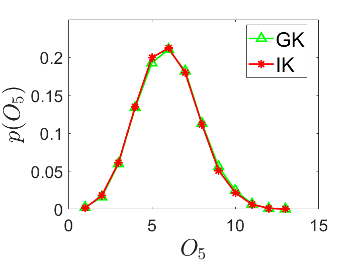
(a) $d=3$

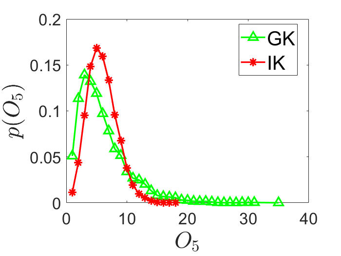
(b) $d=20$

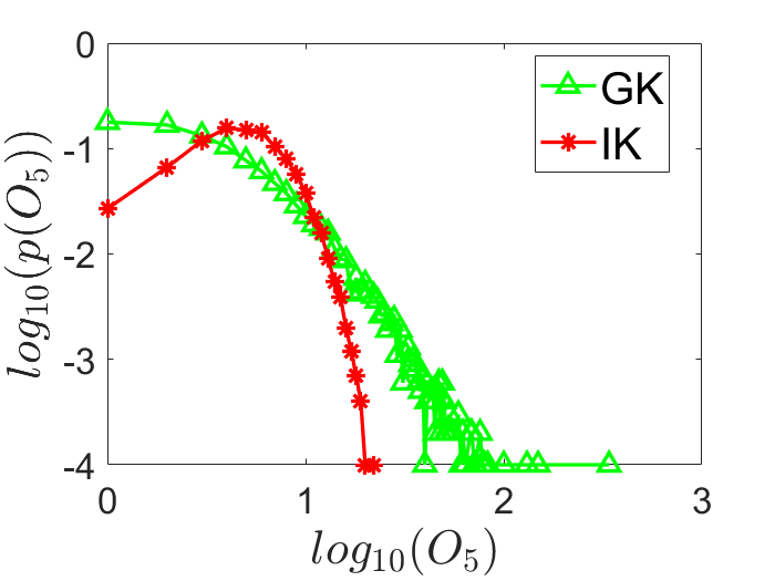
(c) $d=100$

Figure 5. The effect of hubness in $k$-nearest neighbors: GK vs IK. The experiment setting is as used by (Radovanović et al., 2010): a random dataset is drawn uniformly from the unit hypercube $[0,1]^{d}$. The parameter settings used are: $\psi=32$ for IK; $\sigma=5$ for GK.

References

- (1)
- Aggarwal et al. (2001) Charu C. Aggarwal, Alexander Hinneburg, and Daniel A. Keim. 2001. On the surprising behavior of distance metrics in high dimensional space. In Proceedings of the 8th International Conference on Database Theory. 420–434.
- Amsaleg et al. (2019) Laurent Amsaleg, Oussama Chelly, Michael E. Houle, Ken-ichi Kawarabayashi, Milos Radovanovic, and Weeris Treeratanajaru. 2019. Intrinsic Dimensionality Estimation within Tight Localities. In Proceedings of the 2019 SIAM International Conference on Data Mining. 181–189.
- Aryal et al. (2017) Sunil Aryal, Kai Ming Ting, Takashi Washio, and Gholamreza Haffari. 2017. Data-dependent dissimilarity measure: an effective alternative to geometric distance measures. Knowledge and Information Systems 53, 2 (01 Nov 2017), 479–506.
- Bennett et al. (1999) Kristin P. Bennett, Usama Fayyad, and Dan Geiger. 1999. Density-Based Indexing for Approximate Nearest-Neighbor Queries. In Proceedings of the Fifth ACM SIGKDD International Conference on Knowledge Discovery and Data Mining. 233–243.
- Beyer et al. (1999) Kevin S. Beyer, Jonathan Goldstein, Raghu Ramakrishnan, and Uri Shaft. 1999. When Is “Nearest Neighbor” Meaningful?. In Proceedings of the 7th International Conference on Database Theory. Springer-Verlag, London, UK, 217–235.
- Chang and Lin (2011) Chih-Chung Chang and Chih-Jen Lin. 2011. LIBSVM: A library for support vector machines. ACM Transactions on Intelligent Systems and Technology 2 (2011), 27:1–27. Issue 3.
- Chen et al. (2010) Wen-Yen Chen, Yangqiu Song, Hongjie Bai, Chih-Jen Lin, and Edward Y Chang. 2010. Parallel spectral clustering in distributed systems. IEEE transactions on pattern analysis and machine intelligence 33, 3 (2010), 568–586.
- Durrant and Kabán (2009) Robert J. Durrant and Ata Kabán. 2009. When is ‘nearest Neighbour’ Meaningful: A Converse Theorem and Implications. Journal of Complexity 25, 4 (2009), 385–397.
- Ester et al. (1996) Martin Ester, Hans-Peter Kriegel, Jörg Sander, and Xiaowei Xu. 1996. A density-based algorithm for discovering clusters in large spatial databases with noise. In Proceedings of the Second International Conference on Knowledge Discovery and Data Mining. 226–231.
- Fan et al. (2008) Rong-En Fan, Kai-Wei Chang, Cho-Jui Hsieh, Xiang-Rui Wang, and Chih-Jen Lin. 2008. LIBLINEAR: A library for large linear classification. Journal of Machine Learning Research (2008), 1871–1874.
- Felix et al. (2016) X. Y. Felix, A. T. Suresh, K. M. Choromanski, D. N. Holtmann-Rice, and S. Kumar. 2016. Orthogonal random features. In Advances in Neural Information Processing Systems. 1975–1983.
- Francois et al. (2007) Damien Francois, Vincent Wertz, and Michel Verleysen. 2007. The concentration of fractional distances. IEEE Transactions on Knowledge and Data Engineering 19, 7 (2007), 873–886.
- Fukunaga (2013) Keinosuke Fukunaga. 2013. Introduction to Statistical Pattern Recognition (2nd ed.). Academic Press, Chapter 6, section 6.2.
- Gromov and Milman (1983) Mikhael Gromov and Vitali Milman. 1983. A topological application of the isoperimetric inequality. American Journal of Mathematics 105, 4 (1983), 843–854.
- Häkkinen et al. (2020) Antti Häkkinen, Juha Koiranen, Julia Casado, Katja Kaipio, Oskari Lehtonen, Eleonora Petrucci, Johanna Hynninen, Sakari Hietanen, Olli Carpén, Luca Pasquini, et al. 2020. qSNE: quadratic rate t-SNE optimizer with automatic parameter tuning for large datasets. Bioinformatics 36, 20 (2020), 5086–5092.
- Hinneburg et al. (2000) Alexander Hinneburg, Charu C. Aggarwal, and Daniel A. Keim. 2000. What Is the Nearest Neighbor in High Dimensional Spaces?. In Proceedings of the 26th International Conference on Very Large Data Bases. 506–515.
- Houle et al. (2010) Michael E. Houle, Hans-Peter Kriegel, Peer Kröger, Erich Schubert, and Arthur Zimek. 2010. Can Shared-Neighbor Distances Defeat the Curse of Dimensionality?. In Proceedings of the International Conference on Scientific and Statistical Database Management. 482–500.
- Jarvis and Patrick (1973) Raymond A. Jarvis and Edward A. Patrick. 1973. Clustering using a similarity measure based on shared near neighbors. IEEE Trans. Comput. 100, 11 (1973), 1025–1034.
- Jolliffe (2002) I. T. Jolliffe. 2002. Principal Component Analysis. Springer Series in Statistics. New York: Springer-Verlag.
- Kabán (2011) Ata Kabán. 2011. On the Distance Concentration Awareness of Certain Data Reduction Techniques. Pattern Recognition 44, 2 (2011), 265–277.
- Kibriya and Frank (2007) Ashraf M. Kibriya and Eibe Frank. 2007. An Empirical Comparison of Exact Nearest Neighbour Algorithms. In Proceedings of European Conference on Principles of Data Mining and Knowledge Discovery. 140–151.
- Kpotufe (2011) Samory Kpotufe. 2011. K-NN Regression Adapts to Local Intrinsic Dimension. In Proceedings of the 24th International Conference on Neural Information Processing Systems. 729–737.
- Kriegel et al. (2008) Hans-Peter Kriegel, Matthias Schubert, and Arthur Zimek. 2008. Angle-Based Outlier Detection in High-Dimensional Data. In Proceedings of the 14th ACM SIGKDD International Conference on Knowledge Discovery and Data Mining. Association for Computing Machinery, 444–452.
- Ledoux (2001) Michel Ledoux. 2001. The Concentration of Measure Phenomenon. Mathematical Surveys & Monographs, The American Mathematical Society.
- Linderman et al. (2019) George C Linderman, Manas Rachh, Jeremy G Hoskins, Stefan Steinerberger, and Yuval Kluger. 2019. Fast interpolation-based t-SNE for improved visualization of single-cell RNA-seq data. Nature methods 16, 3 (2019), 243–245.
- Liu et al. (2008) Fei Tony Liu, Kai Ming Ting, and Zhi-Hua Zhou. 2008. Isolation forest. In Proceedings of the IEEE International Conference on Data Mining. 413–422.
- Meister and Steinwart (2016) Mona Meister and Ingo Steinwart. 2016. Optimal Learning Rates for Localized SVMs. Journal of Machine Learning Research 17, 1 (2016), 6722–6765.
- Mil'man (1972) Vitali D. Mil'man. 1972. New proof of the theorem of A. Dvoretzky on intersections of convex bodies. Functional Analysis and Its Applications 5, 4 (1972), 288–295.
- Muandet and Schölkopf (2013) Krikamol Muandet and Bernhard Schölkopf. 2013. One-class Support Measure Machines for Group Anomaly Detection. In Proceedings of the Twenty-Ninth Conference on Uncertainty in Artificial Intelligence. 449–458.
- Omohundro (1989) Stephen M Omohundro. 1989. Five balltree construction algorithms. International Computer Science Institute Berkeley.
- Pedregosa et al. (2011) F. Pedregosa, G. Varoquaux, A. Gramfort, V. Michel, B. Thirion, O. Grisel, M. Blondel, P. Prettenhofer, R. Weiss, V. Dubourg, J. Vanderplas, A. Passos, D. Cournapeau, M. Brucher, M. Perrot, and E. Duchesnay. 2011. Scikit-learn: Machine Learning in Python. Journal of Machine Learning Research 12 (2011), 2825–2830.
- Pestov (2000) Vladimir Pestov. 2000. On the geometry of similarity search: Dimensionality curse and concentration of measure. Inform. Process. Lett. 73, 1 (2000), 47–51.
- Qin et al. (2019) Xiaoyu Qin, Kai Ming Ting, Ye Zhu, and Vincent Cheng Siong Lee. 2019. Nearest-Neighbour-Induced Isolation Similarity and Its Impact on Density-Based Clustering. In Proceedings of The Thirty-Third AAAI Conference on Artificial Intelligence. 4755–4762.
- Radovanović et al. (2010) Miloš Radovanović, Alexandros Nanopoulos, and Mirjana Ivanović. 2010. Hubs in Space: Popular Nearest Neighbors in High-Dimensional Data. Journal of Machine Learning Research 11, 86 (2010), 2487–2531.
- Rahimi and Recht (2007) Ali Rahimi and Benjamin Recht. 2007. Random Features for Large-scale Kernel Machines. In Advances in Neural Information Processing Systems. 1177–1184.
- Rodriguez and Laio (2014) Alex Rodriguez and Alessandro Laio. 2014. Clustering by fast search and find of density peaks. Science 344, 6191 (2014), 1492–1496.
- Schölkopf et al. (2001) Bernhard Schölkopf, John C. Platt, John C. Shawe-Taylor, Alex J. Smola, and Robert C. Williamson. 2001. Estimating the Support of a High-Dimensional Distribution. Neural Computing 13, 7 (2001), 1443–1471.
- Shaft and Ramakrishnan (2006) Uri Shaft and Raghu Ramakrishnan. 2006. Theory of Nearest Neighbors Indexability. ACM Transactions on Database Systems 31, 3 (2006), 814–838.
- Talagrand (1996) Michel Talagrand. 1996. A New Look at Independence. The Annals of Probability 24, 1 (1996), 1–34.
- Ting et al. (2021) Kai Ming Ting, Jonathan R. Wells, and Takashi Washio. 2021. Isolation Kernel: The X Factor in Efficient and Effective Large Scale Online Kernel Learning. Data Mining and Knowledge Discovery, https://doi.org/10.1007/s10618-021-00785-1 (2021).
- Ting et al. (2020a) Kai Ming Ting, Bi-Cun Xu, Takashi Washio, and Zhi-Hua Zhou. 2020a. Isolation Distributional Kernel: A New Tool for Kernel Based Anomaly Detection. In Proceedings of the 26th ACM SIGKDD International Conference on Knowledge Discovery and Data Mining. 198–206.
- Ting et al. (2020b) Kai Ming Ting, Bi-Cun Xu, Takashi Washio, and Zhi-Hua Zhou. 2020b. Isolation Distributional Kernel: A New Tool for Point and Group Anomaly Detection. CoRR (2020). https://arxiv.org/abs/2009.12196
- Ting et al. (2018) Kai Ming Ting, Yue Zhu, and Zhi-Hua Zhou. 2018. Isolation Kernel and its effect on SVM. In Proceedings of the 24th ACM SIGKDD International Conference on Knowledge Discovery and Data Mining. ACM, 2329–2337.
- van der Maaten and Hinton (2008) Laurens van der Maaten and Geoffrey E. Hinton. 2008. Visualizing High-Dimensional Data Using t-SNE. Journal of Machine Learning Research 9, 2 (2008), 2579–2605.
- Vinh et al. (2010) Nguyen Xuan Vinh, Julien Epps, and James Bailey. 2010. Information theoretic measures for clusterings comparison: Variants, properties, normalization and correction for chance. The Journal of Machine Learning Research 11 (2010), 2837–2854.
- Wickelmaier (2003) Florian Wickelmaier. 2003. An introduction to MDS. Sound Quality Research Unit, Aalborg University (2003).
- Williams and Seeger (2001) Christopher K. I. Williams and Matthias Seeger. 2001. Using the Nyström Method to Speed Up Kernel Machines. In Advances in Neural Information Processing Systems 13, T. K. Leen, T. G. Dietterich, and V. Tresp (Eds.). MIT Press, 682–688.
- Xu et al. (2019) Bi-Cun Xu, Kai Ming Ting, and Zhi-Hua Zhou. 2019. Isolation Set-Kernel and its application to Multi-Instance Learning. In Proceedings of the 25th ACM SIGKDD International Conference on Knowledge Discovery and Data Mining. 941–949.
- Zelnik-Manor and Perona (2005) Lihi Zelnik-Manor and Pietro Perona. 2005. Self-tuning spectral clustering. In Advances in neural information processing systems. 1601–1608.
- Zhu and Ting (2021) Ye Zhu and Kai Ming Ting. 2021. Improving the Effectiveness and Efficiency of Stochastic Neighbour Embedding with Isolation Kernel. Journal of Artificial Intelligence Research 71 (2021), 667–695.