Peak Infection Time for a Networked SIR Epidemic with Opinion Dynamics

Abstract

We propose an SIR epidemic model coupled with opinion dynamics to study an epidemic and opinions spreading in a network of communities. Our model couples networked SIR epidemic dynamics with opinions towards the severity of the epidemic, and vice versa. We develop an epidemic-opinion based threshold condition to capture the moment when a weighted average of the epidemic states starts to decrease exponentially fast over the network, namely the peak infection time. We define an effective reproduction number to characterize the behavior of the model through the peak infection time. We use both analytical and simulation-based results to illustrate that the opinions reflect the recovered levels within the communities after the epidemic dies out.

I Introduction

The COVID-19 pandemic has caused severe suffering across the world in both public health and the economy. These hardships have motivated researchers from various backgrounds to study the viral pathogenesis, epidemic spreading models, mitigation strategies[1, 2], etc. Besides the COVID-19 pandemic, it is relevant to build dynamic models to study viral spreading processes to predict future outbreaks and to design control algorithms to mitigate the epidemic [3]. One of the popular ways to capture viral spreading processes is by using network-based compartmental models[4]. In networked epidemic models, the infection rates, healing rates, and network structures all play important roles in determining the behaviors of the epidemic spreading processes. Recently, social factors such as human awareness[5], opinion interactions[6], etc., are being taken into consideration when modeling epidemic spreading over networks. In this work, we will consider the classical networked Susceptible-Infected-Recovered (SIR) model coupled with opinion dynamics.

In previous works, researchers have studied the networked SIR models from different perspectives. In [4], the authors study the dynamical behaviors of the networked SIR model, and analyze the threshold conditions for an epidemic to increase or decrease. In [7], the authors leverage testing data to estimate the key parameters of the networked SIR model to design resource allocation methods to mitigate the epidemic.

As mentioned before, people’s beliefs in the seriousness of the epidemic is one important social factor that will have an impact on the spreading process. For example, [8] studies the correlations between the awareness-driven behaviors during the COVID-19 pandemic and the spreading of the COVID-19. Further, [9] constructs a multiplex network with a networked SEIV model coupled with opinion dynamics, then explores the disease-free equilibrium. Inspired by the health-belief model developed by social scientists [10], where people’s behavior in the pandemic will be influenced by their beliefs in the seriousness of the epidemic, [6] and [11] develop a networked SIS model with cooperative opinion dynamics, and both cooperative and antagonistic opinion dynamics, respectively. The authors in [6] study both the disease-free and non-disease-free equilibria of the model. Our previous work, [11], defines an opinion-dependent reproduction number to explore further the effect of the antagonistic opinions in epidemic spreading. Based on the health-belief model, we will develop a networked SIR model coupled with cooperative opinion dynamics.

The main contributions of this work can be summarized as follows: we define a networked SIR epidemic model coupled with opinion dynamics. Then, we develop two concepts: an effective reproduction number and a peak infection time. We utilize the effective reproduction number to explore epidemic spreading by studying the peak infection time. In particular, different from the previous works [6, 11], where stability and convergence of the equilibria are the main focuses, this work emphasizes more on exploring the transient behavior of the epidemic, characterized by the effective reproduction number and the peak infection time. Additionally, we further analyze the opinion states via the behavior of the epidemic.

We organize the paper as follows: In Section II, we introduce the networked SIR model coupled with opinion dynamics and formulate the problems of interest; Section III studies the equilibrium of the developed model. Based on the model, Section III defines the effective reproduction number and peak infection time. Section III further explores the epidemic’s dynamical behavior by relating the effective reproduction number and the peak infection time. Section IV illustrates the results of the paper through simulations. Section V concludes the paper and outlines research directions.

Notation

For any positive integer $n$, we use $[n]$ to denote the index set $\left\{1,2,\ldots,n\right\}$. We view vectors as column vectors and write $x^{\top}$ to denote the transpose of a column vector $x$. For a vector $x$, we use $x_{i}$ to denote the $i$th entry. For any matrix $M\in{\rm I\!R}^{n\times n}$, we use $[M]_{i,:}$, $[M]_{:,j}$, $[M]_{ij}$, to denote its $i$th row, $j$th column and $ij$th entry, respectively. We use $\tilde{M}=\text{diag}\left\{m_{1},\ldots,m_{n}\right\}$ to represent a diagonal matrix $\tilde{M}\in{\rm I\!R}^{n\times n}$ with $[\tilde{M}]_{ii}=m_{i}$, $\forall i\in\left[n\right]$. We use $\boldsymbol{0}$ and $\boldsymbol{1}_{n}$ to denote the vectors whose entries all equal 0 and 1, respectively, and $I$ to denote the identity matrix. The dimensions of the vectors and matrices are to be understood from the context.

For a real square matrix $M$, we use $\rho\left(M\right)$ and $\sigma\left(M\right)$ to denote its spectral radius and spectral abscissa (the largest real part among its eigenvalues), respectively. For any two vectors $v,w\in{\rm I\!R}^{n}$, we write $v\geq w$ if $v_{i}\geq w_{i}$, and $v\gg w$ if $v_{i}>w_{i}$, $\forall i\in\left[n\right]$. The comparison notations between vectors are used for matrices as well, for instance, for $A,B\in{\rm I\!R}^{n\times n}$, $A\gg B$ indicates that $A_{ij}>B_{ij}$, $\forall i,j\in\left[n\right]$.

Consider a directed graph $\mathcal{G}=\left(\mathcal{V},\mathcal{E}\right)$, with the node set $\mathcal{V}=\left\{v_{1},\ldots,v_{n}\right\}$ and the edge set $\mathcal{E}\subseteq\mathcal{V}\times\mathcal{V}$. Let matrix $A\in{\rm I\!R}^{n\times n}$, $[A]_{ij}=a_{ij}$, denote the adjacency matrix of $\mathcal{G}=\left(\mathcal{V},\mathcal{E}\right)$, where $a_{ij}\in{\rm I\!R}_{>0}$ if $\left(v_{j},v_{i}\right)\in\mathcal{E}$ and $a_{ij}=0$ otherwise. Graph $\mathcal{G}$ does not allow self-loops, i.e., $a_{ii}=0,$ $\forall i\in\left[n\right]$. Let $k_{i}=\sum_{j\in\mathcal{N}_{i}}\left|a_{ij}\right|$, where $\mathcal{N}_{i}=\left\{\left.v_{j}\right|\left(v_{j},v_{i}\right)\in\mathcal{E}\right\}$ denotes the neighbor set of $v_{i}$ and $\left|a_{ij}\right|$ denotes the absolute value of $a_{ij}$. The graph Laplacian of $\mathcal{G}$ is defined as $L\triangleq\tilde{K}-A$, where $\tilde{K}\triangleq\text{diag}\left\{k_{1},\ldots,k_{n}\right\}$.

II Modeling and Problem Formulation

In this section, we introduce the networked SIR model coupled with opinion dynamics. We also formulate the problem to be analyzed in this work.

We start by defining a disease transmission network $\mathcal{G}=\left(\mathcal{V},\mathcal{E}\right)$ as a weighted directed graph with a node set $\mathcal{V}=\left\{v_{1},\ldots,v_{n}\right\}$ representing $n$ disjoint communities and the edge set $\mathcal{E}\subseteq\mathcal{V}\times\mathcal{V}$ representing disease-transmitting contacts over $\mathcal{V}$. We denote the weight of each edge $(v_{j},v_{i})$ as $\beta_{ij}$. Then, a basic continuous-time networked SIR model on graph $\mathcal{G}$, which was studied in [4], can be defined as:

$$\dot{s_{i}}\left(t\right) =-s_{i}\left(t\right)\sum_{j\in\mathcal{N}_{i}}\beta_{ij}x_{j}\left(t\right),$$ (1a)

$$\dot{x_{i}}\left(t\right) =s_{i}\left(t\right)\sum_{j\in\mathcal{N}_{i}}\beta_{ij}x_{j}\left(t\right)-\gamma_{i}x_{i}\left(t\right),$$ (1b)

$$\dot{r}_{i}\left(t\right) =\gamma_{i}x_{i}\left(t\right),$$ (1c)

where $(s_{i}(t),x_{i}(t),r_{i}(t))\in[0,1]$, $\forall i\in[n]$ are the states indicating the proportion of susceptible, infected, and recovered population in community $i\in[n]$ at time $t\geq 0$, respectively. Moreover, $\beta_{ij}\in\mathbb{R}_{\geq 0}$ is the transmission rate from community $j$ to $i$, and $\gamma_{i}\in\mathbb{R}_{\geq 0}$ is the recovery rate of community $i$. Note that (1a)-(1c) satisfy $s(t)+x(t)+r(t)=1\ \forall t\geq t_{0}\in\mathbb{R}_{\geq 0}$ as a result of the assumption that $\exists t_{0}\in\mathbb{R}_{\geq 0}$ such that $s(t_{0})+x(t_{0})+r(t_{0})=1$ and $\dot{s}(t)+\dot{x}(t)+\dot{r}(t)=0\ \forall t\in\mathbb{R}_{\geq 0}$.

Similarly, we define the opinion spreading network as a directed graph $\bar{\mathcal{G}}=\left(\mathcal{V},\bar{\mathcal{E}}\right)$, where the edge set $\bar{\mathcal{E}}\subseteq\mathcal{V}\times\mathcal{V}$ represents the opinion-disseminating interactions over the same $n$ communities. Each edge in the graph is weighted by $\bar{a}_{ij}\in\mathbb{R}_{\geq 0}$ indicating the opinion-disseminating influence from node $j$ to node $i$. Let $o_{i}(t)\in[0,1]$, $\forall i\in[n]$, $t\geq 0$, denote the belief of community $i$ on the severity of the epidemic at time $t$, where $o_{i}(t)=1$ indicates community $i$ considers the epidemic to be extremely serious, while $o_{i}(t)=0$ implies community $i$ believes the epidemic is not serious at all. We adapt Abelson’s models of opinion dynamics from [12, Equation (10)], where $\bar{\mathcal{N}}_{i}=\left\{\left.v_{j}\right|\left(v_{j},v_{i}\right)\in\bar{\mathcal{E}}\right\}$:

$$\dot{o}_{i}\left(t\right)=\sum_{j\in\mathcal{\bar{N}}_{i}}\bar{a}_{ij}\left(o_{j}\left(t\right)-o_{i}\left(t\right)\right).$$ (2)

We assume that the $n$ communities share a homogeneous minimum incoming transmission rate $\beta_{\min}$ and a homogeneous recovery rate $\gamma_{\min}$, where $\beta_{\min}$ corresponds to the strongest belief of a community in the severity of the epidemic $o_{i}(t)=1$, while $\gamma_{\min}$ corresponds to the weakest belief of a community in the severity of the epidemic $o_{i}(t)=0$. To couple the networked SIR model with the opinion dynamics, we employ the health-belief model, which is the best known and most widely used theory in health behavior research [10]. The health-belief model proposes people’s beliefs about health problems, perceived benefits of actions, and/or perceived barriers to actions that can explain their engagement, or lack thereof, in health-promoting behavior. Therefore, people’s beliefs in their perceived susceptibility and/or in their perceived severity of the illness affect how susceptible they are and/or how effective they will be at healing from these epidemics. We define a networked SIR model influenced by the opinion dynamics as:

$$\dot{s_{i}}\left(t\right) =-s_{i}\left(t\right)\sum_{j\in\mathcal{N}_{i}}\left(\beta_{ij}-(\beta_{ij}-\beta_{\min})o_{i}(t)\right)x_{j}\left(t\right),$$ (3a)

$$\dot{x_{i}}\left(t\right) =s_{i}\left(t\right)\sum_{j\in\mathcal{N}_{i}}\left(\beta_{ij}-(\beta_{ij}-\beta_{\min})o_{i}(t)\right)x_{j}\left(t\right)$$

$$\ \ \ \ -\left(\gamma_{\min}+(\gamma_{i}-\gamma_{\min})o_{i}(t)\right)x_{i}\left(t\right).$$ (3b)

In (3a) and (3b), the transmission rate of community $i$, is obtained through the linear interpolation between $\beta_{ij}$ and $\beta_{min}$ scaled by the level of community $i$’s belief in the seriousness of the epidemic, $o_{i}(t)$. A higher $o_{i}(t)$ will lead to lower transmission rates for community $i$. A similar interpretation can apply to the healing rate of community $i$ which is scaled by the level of community $i$’s belief in the seriousness of the epidemic, with a higher opinion state leading to a higher healing rate of community $i$.

Notice that $(1-s_{i}(t))=x_{i}(t)+r_{i}(t)$, $t\geq 0$, $\forall i\in[n]$, captures the proportion of the population that are infected/have been infected with the epidemic. Hence, $(1-s_{i}(t))$ captures the infection level within community $i$. By modifying the opinion dynamics in (2) via cooperating the infection level:

$$\dot{o_{i}}\left(t\right)=\left(1-s_{i}\left(t\right)-o_{i}\left(t\right)\right)+\sum_{j\in\bar{\mathcal{N}}_{i}}\left(o_{j}\left(t\right)-o_{i}\left(t\right)\right),$$ (4)

where a higher proportion of the infected plus recovered population within community $i$ will lead to a stronger belief in the seriousness of the epidemic, and vice versa.

We have presented the epidemic-opinion model in (3a)-(4), then, we can state the problem of interest in this work. We are interested in exploring the mutual influence between the epidemic spreading over the graph $\mathcal{G}$ of $n$ communities in (3a) and (3b), and the opinions of the $n$ communities about the epidemic captured by graph $\bar{\mathcal{G}}$ in (4). In this paper, we will:

1. analyze the equilibria of the system in (3a)-(4). In particular, we connect the opinion states at the equilibrium to the infection level of the communities;

2. define an effective reproduction number to characterize the spreading of the disease. In particular, we explore the transient behavior of the epidemic-opinion model by leveraging peak infection time;

3. illustrate the results through simulations.

The analysis presented in this work can provide insights for decision-makers who aim to analyze disease spreading and its coupling with the public’s opinion towards the epidemic.

III Main Results

This section examines the mutual influence between the epidemic dynamics in (3a) and (3b), and the opinion dynamics in (4). Particularly, we construct the compact form of the incorporated system to define an effective reproduction number to explore the peak infection time of the model. We also analyze the evolution of the epidemic by using the effective reproduction number and peak infection time.

We write (3a), (3b), and (4) in a compact form as follows:

$$\dot{s}\left(t\right) =-\left(\tilde{S}\left(t\right)\left(B-\tilde{O}\left(t\right)\left(B-B_{\min}\right)\right)\right)x\left(t\right),$$ (5a)

$$\dot{x}\left(t\right) =\left(\tilde{S}\left(t\right)\left(B-\tilde{O}\left(t\right)\left(B-B_{\min}\right)\right)\right)x\left(t\right)$$

$$\ \ \ \ \ -\left(G_{\min}+\left(G-G_{\min}\right)\tilde{O}\left(t\right)\right)x\left(t\right),$$ (5b)

$$\dot{o}\left(t\right) =\left(\boldsymbol{1}_{n}-s\left(t\right)\right)-\left(\bar{L}+I_{n}\right)o\left(t\right),$$ (5c)

where $\tilde{S}\left(t\right)=\text{diag}\left(s\left(t\right)\right)$, $\tilde{O}\left(t\right)=\text{diag}\left(o\left(t\right)\right)$, $G_{\min}$ and $G$ are diagonal matrices, with $\left[G_{\min}\right]_{ii}=\gamma_{\min}$, and $[G]_{ii}=\gamma_{i}$, $\forall i\in[n]$. Note that $\bar{L}$ is the Laplacian matrix of the opinion spreading graph $\mathcal{\bar{G}}$. By defining $B\left(o(t)\right)=(B-\tilde{O}\left(t\right)\left(B-B_{\min}\right))$, $G\left(o(t)\right)=(G_{\min}+\left(G-G_{\min}\right)\tilde{O}\left(t\right))$,

$$\dot{s}\left(t\right) =-\left(\tilde{S}\left(t\right)B\left(o(t)\right)\right)x\left(t\right),$$ (6a)

$$\dot{x}\left(t\right) =\tilde{S}\left(t\right)B\left(o(t)\right)x\left(t\right)-G\left(o(t)\right)x\left(t\right).$$ (6b)

For the epidemic spreading process, we assume that community $i$ can pass the virus to community $j$ through at least one directed path in the network $\mathcal{G}$, $\forall i,j\in[n]$, $i\neq j$. For the opinion spreading process, we assume that community $i$ can affect community $j$’s opinion through at least one directed path in $\mathcal{\bar{G}}$. Therefore, we have the following assumption for the epidemic and opinion spreading over the communities:

Assumption 1.

Suppose $\forall i\in[n]$, $s_{i}(0),x_{i}(0),o_{i}(0)\in[0,1]$, $s_{i}(0)+x_{i}(0)+r_{i}(0)=1$, $\gamma_{i}\geq\gamma_{{\rm min}}>0$, and $\beta_{ij}\geq\beta_{{\rm min}}>0$, $\forall j\in\mathcal{N}_{i}$. Further, both $\mathcal{G}$ and $\bar{\mathcal{G}}$ are strongly connected.

III-A Equilibrium

First we show the model in (5a)-(5c) is well-defined.

Lemma 1.

For the epidemic-opinion model in (5a)-(5c), if $(s_{i}(0),x_{i}(0),o_{i}(0))\in[0,1]$, and $s_{i}(0)+x_{i}(0)+r_{i}(0)=1$, then $(s_{i}(t),x_{i}(t),o_{i}(t))\in[0,1]$, $\forall t>0$, $\forall i\in[n]$.

The system defined in (5a)-(5c) is a group of polynomial ODEs defined over the compact set $[0,1]^{3n}$. Hence, the system is Lipschitz over $[0,1]^{3n}$. To prove Lemma 1, we can show that all gradient vector fields on the boundary of the set $[0,1]^{3n}$ are either pointing towards the set’s interior or tangential to the boundary [13]. The proof is similar to the proof of [11, Lemma 7] and thus omitted here.

Lemma 2.

If $s_{i}(0),x_{i}(0),o_{i}(0)\in[0,1]$, $\forall i\in[n]$, the susceptible states, $s_{i}(t)$, are monotonically decreasing.

Proof.

Lemma 1 indicates that $x(t)\in[0,1]^{n}$ $\forall t\geq 0$. From Assumption 1, the matrix $-(\tilde{S}(t)(B-\tilde{O}(t)(B-B_{\min})))$ is non-positive, therefore, the RHS of (5a) is always non-positive, which completes the proof. ∎

After considering the monotonicity of the susceptible population, we move to the next lemmas to study the equilibria of the epidemic-opinion model.

Lemma 3.

The equilibria of the epidemic-opinion model in (5a)-(5c) take the form $(s_{e},\boldsymbol{0},(\bar{L}+I_{n})^{-1}(\boldsymbol{1}_{n}-s_{e}))$, where $[s_{e}]_{i}\in[0,1]$ and $[(\bar{L}+I_{n})^{-1}(\boldsymbol{1}_{n}-s_{e}))]_{i}\in[0,1]$, $\forall i\in[n]$.

Proof.

Based on Lemma 2, the RHS of (5a) is always less than or equal to zero. Therefore, the susceptible states are monotonically decreasing. To compute the equilibria of the system in (5a)-(5c), let $\dot{s}(t)=\dot{x}(t)=\dot{o}(t)=\boldsymbol{0}$, which leads to $x_{e}=\boldsymbol{0}$, and $s_{e}$ can be any point located in the set $[0,1]^{n}$. Substituting the equilibrium point $s_{e}$ into (5c) with $\dot{o}(t)=\boldsymbol{0}$,

$$\boldsymbol{0}=(\boldsymbol{1}_{n}-s_{e})-\left(\bar{L}+I_{n}\right)o_{e}.$$ (7)

Since the row sums of the Laplacian matrix $L$ are zeros, the matrix $(\bar{L}+I_{n})$ is a strictly diagonally dominant matrix, i.e., the matrix $(\bar{L}+I_{n})$ is positive definite. Therefore,

$$o_{e}=\left(\bar{L}+I_{n}\right)^{-1}\left(\boldsymbol{1}_{n}-s_{e}\right).$$ (8)

Now we have to show that for each $s_{e}\in[0,1]^{n}$, the solution $o_{e}\in[0,1]^{n}$. Rearrange (7) as follows:

$$\left(\boldsymbol{1}_{n}-s_{e}\right)=\left(\bar{L}+I_{n}\right)o_{e}.$$

If $s_{e}\in[0,1]^{n}$, we have $(\boldsymbol{1}_{n}-s_{e})\in[0,1]^{n}$, which leads to $\left(\bar{L}+I_{n}\right)o_{e}\in[0,1]^{n}$.

We prove $[o_{e}]_{i}\in[0,1]$ $\forall i\in[n]$ by contradiction. Without loss of generality, suppose that $[o_{e}]_{i}>1$, with $[o_{e}]_{i}-a_{i}=1$, belongs to a solution to the $i$th row of the equation $\left(\boldsymbol{1}_{n}-s_{e}\right)=\left(\bar{L}+I_{n}\right)o_{e}$. As shown before, the matrix $\left(\bar{L}+I_{n}\right)$ is strictly diagonally dominant and $\bar{L}_{ii}+\sum_{j\in\mathcal{N}_{i}}\bar{L}_{ij}+1=1$, $\forall i\in[n]$. If the rest of the entries of the solution $[o_{e}]_{j}\leq[o_{e}]_{i}$, $j\neq i$, $j\in[n]$, we must have $[\left(I_{n}\right)o_{e}]_{i}>1$, which violates $(\boldsymbol{1}_{n}-s_{e})\in[0,1]^{n}$. Hence, to ensure the $i$th entry $[\left(\bar{L}+I_{n}\right)o_{e}]_{i}\in[0,1]$, there must be an entry $[o_{e}]_{j}>[o_{e}]_{i}$ in the solution $o_{e}$ such that $[o_{e}]_{j}-a_{j}=1$, where $a_{j}>a_{i}$, $j\in[n],j\neq i$.

Then, consider the $j$th row of the equation $\left(\boldsymbol{1}_{n}-s_{e}\right)=\left(\bar{L}+I_{n}\right)o_{e}$. To ensure the solution of the $j$th row belongs to $[0,1]$, based on the same analysis technique, there must exist one entry $[o_{e}]_{k}$ such that $[o_{e}]_{k}>1$, with $[o_{e}]_{k}-a_{k}=1$, $a_{k}>a_{j}>a_{i}$. Following the same process to check the rest of the rows of the equation, we can conclude that, for the last equation left to check, there is no such entry left in $o_{e}$ satisfying the inequality condition, $a_{l}>\dots>a_{k}>a_{j}>a_{i}$, where $[o_{e}]_{l}$ corresponds to the last row left to be checked in the equation $(\boldsymbol{1}_{n}-s_{e})=(\bar{L}+I_{n})o_{e}$, with $[o_{e}]_{l}-a_{l}=1$. Therefore, each entry of $o_{e}$ as a solution to $\left(\boldsymbol{1}_{n}-s_{e}\right)=\left(\bar{L}+I_{n}\right)o_{e}$ is not greater than 1. Using the same analysis technique, it can be shown that each entry of $o_{e}$ as a solution to $\left(\boldsymbol{1}_{n}-s_{e}\right)=\left(\bar{L}+I_{n}\right)o_{e}$ is not smaller than 0. Therefore, the solution $o_{e}$ to the equation $\left(\boldsymbol{1}_{n}-s_{e}\right)=\left(\bar{L}+I_{n}\right)o_{e}$ must be located in $[0,1]^{n}$, which proves the statement. ∎

Lemma 3 shows that there are infinite equilibria for the epidemic-opinion model captured by (5a)-(5c). In particular, (8) indicates that the opinion states of the communities at the equilibrium can be uniquely evaluated as a function of the steady-state susceptible population in the communities. The following lemma further characterizes the condition that the communities reach a consensus on their opinions, i.e., the opinion states are the same when the epidemic disappears.

Lemma 4.

The communities will reach consensus on their opinions if and only if all the communities have the same proportion of infections, captured by the equilibria $\left(s_{e},\boldsymbol{0},\boldsymbol{1}_{n}-s_{e}\right)$, where $[s_{e}]_{i}=[s_{e}]_{j}\ \forall i\neq j$.

Proof.

First, we show the necessary condition. If all communities reach consensus at the equilibrium point, giving that $o_{e}$ is a consensus state, where $[o_{e}]_{i}=[o_{e}]_{j}$, $\forall i,j\in[n]$, $i\neq j$, then $Lo_{e}=\boldsymbol{0}$. From (7), $s_{e}=\boldsymbol{1}_{n}-o_{e}$, which implies that $[s_{e}]_{i}=1-[o_{e}]_{i}$, and $[s_{e}]_{i}=[s_{e}]_{j}$, $\forall i,j\in[n]$, $i\neq j$.

For the sufficient condition, if all communities have the same proportion of the infected population at the equilibria, we have $1-[s_{e}]_{i}=1-[s_{e}]_{j}$, $\forall i,j\in[n]$, $i\neq j$. Based on (7), we have $\boldsymbol{1}_{n}-s_{e}=(\bar{L}+I_{n})o_{e}$. Since $\left(\bar{L}+I_{n}\right)$ is a positive definite matrix, $o_{e}=\left(\bar{L}+I_{n}\right)^{-1}(\boldsymbol{1}_{n}-s_{e})$ is the unique solution to the equation. Further, $L$ is positive semi-definite with only one zero eigenvalue, paired with the eigenvector $v$, where all the entries of $v$ are the same. Therefore, $\left(\bar{L}+I_{n}\right)v=v$, giving that $v=o_{e}=(\boldsymbol{1}_{n}-s_{e})$ is the unique solution to the equation $\left(\bar{L}+I_{n}\right)o_{e}=\boldsymbol{1}_{n}-s_{e}$, completing the proof. ∎

Lemma 3 and Lemma 4 summarize the equilibria of the epidemic-opinion model from (5a) to (5c). In particular, the lemmas show that the communities’ beliefs in the seriousness of the epidemic can reflect the infection level. More importantly, the communities will reach consensus on the seriousness of the epidemic if and only if the epidemic caused the same proportion of infected population in all communities. Under this situation, the belief on the seriousness of the epidemic is proportional to the proportion of the recovered population in all communities, characterized by $o_{e}=\boldsymbol{1}_{n}-s_{e}$.

Remark 1.

The communities can rarely reach a consensus of their opinions on the epidemic’s severity since it will be implied by Lemma 4 that every community has the same infection level, which is unusual. However, one exception is when every community is fully infected, then all communities will agree that the epidemic is utterly severe ($o_{e}=\boldsymbol{1}_{n}$).

III-B Effective Reproduction Number

The effective reproduction number of the model characterizes the dynamical behavior of the system. We introduce the following lemmas before formally defining the notion.

Lemma 5.

[14, Thm. 2.7, and Lemma 2.4] Suppose that M is an irreducible nonnegative matrix. Then:

1. M has a simple positive real eigenvalue equal to its spectral radius, $\rho(M)$;

2. There is a unique (up to scalar multiple) left eigenvector $v\gg\boldsymbol{0}$ (right eigenvector $w\gg\boldsymbol{0}$) pairing with $\rho(M)$;

3. $\rho(M)$ increases when any entry of M increases;

4. If N is also an irreducible nonnegative matrix with the same size and $M\geq N$, then $\rho(M)\geq\rho(N)$.

Lemma 6.

[15, Prop. 1] Suppose that $\varLambda$ is a negative diagonal matrix in ${\rm I\!R}^{n\times n}$ and $N$ is an irreducible nonnegative matrix in ${\rm I\!R}^{n\times n}$. Let $M=\varLambda+N$. Then, $\sigma(M)<0$ if and only if $\rho(-\varLambda^{-1}N)<1$, $\sigma(M)=0$ if and only if $\rho(-\varLambda^{-1}N)=1$, and $\sigma(M)>0$ if and only if $\rho(-\varLambda^{-1}N)\leavevmode\nobreak\ >\leavevmode\nobreak\ 1$.

Lemma 7.

[14, Sec. 2.1 and Lemma 2.3] Suppose that $M$ is an irreducible Metzler matrix. Then, $\sigma\left(M\right)$ is a simple eigenvalue of $M$ and there exists a unique (up to scalar multiple) left eigenvector $x\gg\boldsymbol{0}$ (right eigenvector $y\gg\boldsymbol{0}$) such that $x^{\top}M=\sigma\left(M\right)x$ ($My=\sigma\left(M\right)y$).

Lemma 8.

[16, Sec. 1, Lemma 2] Suppose that $A,B\in{\rm I\!R}^{n\times n}$ are Metzler matrices. Then, $\sigma\left(A\right)\leq\sigma\left(B\right)$ if $A\leq B$.

Definition 1.

[Effective Reproduction Number $R_{o}(t)$] Let $R_{o}(t)=\rho(G^{-1}(o(t))\tilde{S}(t)B(o(t)))$, $\forall t\geq 0$, denote the Effective Reproduction Number, where $G(o(t))$, $\tilde{S}(t)$, and $B(o(t))$ are defined in (5b).

Note that the effective reproduction number $R_{o}(t)$ depends not only on the proportion of the susceptible population $s(t)$, but also on the variation of the opinion states $o\left(t\right)$.

Proposition 1.

The Effective Reproduction Number $R_{o}(t)$ has the following properties:

1. If

   $$G^{-1}(o(t_{1}))\tilde{S}(t_{1})B(o(t_{1}))\geq G^{-1}(o(t_{0}))\tilde{S}(t_{0})B(o(t_{0})),$$

   then $R_{o}(t_{1})\geq R_{o}(t_{0})$;

2. $R_{o}(t)$ is strictly monotonically decreasing with respect to $s(t)$, $\forall t\geq 0$;

3. If $o\left(t_{0}\right)\leq o\left(t_{1}\right)$, $\forall t_{0}<t_{1}$, then $R_{o}(t_{1})\leq R_{o}(t_{0})$.

Proof.

1) Based on Assumption 1, and the definitions of $G(o(t))$ and $\tilde{S}(t)$, we conclude that $G(o(t))$ and $\tilde{S}(t)$ are positive definite diagonal matrices, and $B(o(t))$ is an irreducible nonnegative matrix, $\forall t\geq 0$. Hence, $G^{-1}(o(t))\tilde{S}(t)B(o(t))$ is an irreducible nonnegative matrix. For statement 1), if

$$G^{-1}(o(t_{1}))\tilde{S}(t_{1})B(o(t_{1}))\geq G^{-1}(o(t_{0}))\tilde{S}(t_{0})B(o(t_{0})),$$

based on Lemma 5,

$$\rho(G^{-1}(o(t_{1}))\tilde{S}(t_{1})B(o(t_{1})))\geq\rho(G^{-1}(o(t_{0}))\tilde{S}(t_{0})B(o(t_{0}))),$$

which leads to $R_{o}(t_{1})\geq R_{o}(t_{0})$.

2) $R_{o}(t)$ is strictly monotonically decreasing with respect to $s(t)$ means that, when $o(t)$ is fixed, a decrease in $s(t)$ leads to a decrease in $R_{o}(t)$, $\forall t\geq 0$. Without loss of generality, assume that $o(t_{0})=o(t_{1})$, and $t_{0}<t_{1}$. From Lemma 2, the proportion of infected population for each community is monotonically decreasing. Thus, $s(t_{1})\leq s(t_{0})$, and $[\tilde{S}(t_{1})]_{ii}\leq[\tilde{S}(t_{0})]_{ii}$, $\forall i\in[n]$, which leads to

$$\left[G\left(o\left(t_{0}\right)\right)^{-1}\tilde{S}(t_{0})B\left(o\left(t_{0}\right)\right)\right]_{i,:}\geq\left[G\left(o\left(t_{1}\right)\right)^{-1}\tilde{S}(t_{1})B\left(o\left(t_{1}\right)\right)\right]_{i,:}$$

where other entries of both matrices remain the same. Based on statement 1) of this proposition, $R_{o}(t_{1})\leq R_{o}(t_{0})$, implying that $R_{o}(t)$ is monotonically decreasing with respect to $s(t)$.

3) When $o\left(t_{0}\right)\leq o\left(t_{1}\right)$, $\forall t_{0}<t_{1}$, we have

$$[G^{-1}\left(o\left(t_{0}\right)\right)]_{ii}\geq[G^{-1}\left(o\left(t_{1}\right)\right)]_{ii},$$

$$[B\left(o\left(t_{0}\right)\right)]_{i,:}\geq[B\left(o\left(t_{1}\right)\right)]_{i,:},$$

where other entries of the matrices $G^{-1}\left(o\left(t_{1}\right)\right)$ and $B\left(o\left(t_{1}\right)\right)$ are equal to $G^{-1}\left(o\left(t_{0}\right)\right)$ and $B\left(o\left(t_{1}\right)\right)$, respectively. Additionally, from Lemma 2, $\forall t_{0}<t_{1}$, we have $\tilde{S}_{ii}(t_{1})\leq\tilde{S}_{ii}(t_{0})$. Following the same analysis technique from the proof of statement 2), we have that $R_{o}(t_{1})\leq R_{o}(t_{0})$. ∎

The effective reproduction number is influenced by both the opinion states and the proportion of the susceptible population. In particular, when the opinions are fixed, the susceptible proportion will always ensure that the effective reproduction number decreases, since the recovered population will not be infected again. The opinion states will also have an influence on the change of the effective reproduction number in both directions: higher opinion states will lead to a lower effective reproduction number, and vice versa. As we mentioned in Section II, communities with stronger beliefs in the seriousness of the epidemic will take actions to avoid infections, leading to a lower effective reproduction number, and vice versa. Further, when all communities think the epidemic is extremely serious, $o_{\max}(t)=\boldsymbol{1}_{n},\forall t\geq 0$. When all communities think the epidemic is not worth treating at all during the pandemic, $o_{\min}(t)=\boldsymbol{0}$, $\forall t\geq 0$. Under the two extreme situations, the effective reproduction number satisfies the following result.

Corollary 1.

For all $t\geq 0$, the effective reproduction number $R_{o}(t)$ satisfies $R_{\min}(t)\leq R_{o}(t)\leq R_{\max}(t)$, where

$$R_{\min}(t)=\rho\left(G^{-1}\left(o_{\max}\right)\tilde{S}\left(t\right)B\left(o_{\max}\right)\right),$$

and

$$R_{\max}(t)=\rho\left(G^{-1}\left(o_{\min}\right)\tilde{S}(t)B\left(o_{\min}\right)\right).$$

The proof of Corollary 1 is similar to the proof of Proposition 1, thus omitted here. Corollary 1 indicates that, given any time $t$, if the proportion of the susceptible population of each community are the same, the effective reproduction number is determined by the opinion states, where stronger beliefs in the seriousness of the epidemic lead to a lower effective reproduction number, and vice versa. Compared to the classical SIR model[17], where the effective reproduction number is monotonically decreasing with respect to the decreasement of the proportion of the susceptible population, under the influence of the opinions, the $R_{o}(t)$ defined in this work may not monotonically decrease. Therefore, $R_{o}(t)$ can lead to more diverse behaviors in the epidemic spreading process. In order to analyze the dynamical behavior of the epidemic-opinion model, we define a concept called peak infection time to characterize the influence of the effective reproduction number $R_{o}(t)$ in determining the behavior of the epidemic.

III-C Peak Infection Time

To connect the effective reproduction number $R_{o}(t)$ to the behavior of the epidemic-opinion model, we denote

$$\sigma(t)=\sigma(\tilde{S}(t)B(o(t))-G(o(t)))$$ (9)

and $p(t)$ as the spectral abscissa of $(\tilde{S}(t)B(o(t))-G(o(t)))$ and the corresponding normalized left eigenvector $\forall t\geq 0$, respectively. From Assumption 1 and Lemma 7, $(\tilde{S}(t)B(o(t))-G(o(t)))$ is an irreducible Metzler matrix, thus $\sigma(t)$, $\forall t\geq 0$, is a positive real eigenvalue. Additionally, the normalized left eigenvector $p(t)$ satisfies $p(t)\gg\boldsymbol{0}$ and $p^{\top}(t)\boldsymbol{1}_{n}=1$, $\forall t\geq 0$. Then, we define a weighted average of the epidemic states, for a given $t_{1}\in[t_{0},t_{2}]$, $p^{\top}(t_{1})x(t)$ as a metric to reflect the trend of the epidemic over the time interval $[t_{0},t_{2}]$. Based on the properties of $\sigma(t)$ and $p(t)$, we have $p^{\top}(t_{1})x(t)\geq 0$, $\forall t\geq 0$ and $p^{\top}(t_{1})x(t)=0$ if and only if $x(t)=\boldsymbol{0}$. Therefore, $p^{\top}(t_{1})x(t)$ reflects the overall trend of the epidemic spreading over the time interval $[t_{0},t_{2}]$, and $p^{\top}(t_{1})x(t)=0$ if and only if the epidemic has died out.

Definition 2.

[Peak Infection Time $t_{p}$] A Peak Infection Time $t_{p}$ is defined as a turning point, where $p^{\top}(t_{p})x(t)$ is increasing for all $t\in[t_{0},t_{p})$ and $p^{\top}(t_{p})x(t)$ is decreasing for all $t\in(t_{p},t_{1}]$, for sufficiently small time intervals $(t_{p}-t_{0})>0$ and $(t_{1}-t_{p})>0$.

The peak infection time describes a point in time where the weighted average of the infected proportions $p^{\top}(t_{p})x(t)$ over the communities reaches a local peak value over the time interval $[t_{0},t_{1}]$.

Theorem 1.

Given a peak infection time $t_{p}$, we have $R_{o}(t_{p})=1$, $R_{o}(t)>1$, for $t\in[t_{0},t_{p})$ and $R_{o}(t)<1$, for $t\in(t_{p},t_{1}]$, for $t_{p}-t_{0}>0$ and $t_{1}-t_{p}>0$ sufficiently small.

Proof.

First we show that for a peak infection time $t_{p}$, we have $R_{o}(t_{p})=1$. Since $\frac{d}{dt}(p^{\top}(t_{p})x(t))$ is a continuous function over the time interval $[t_{0},t_{1}]$, based on Definition 2, $p^{\top}(t_{p})x(t)$ is increasing for all $t\in[t_{0},t_{p})$ and decreasing for all $t\in(t_{p},t_{1}]$. Therefore, by continuity, $\frac{d}{dt}(p^{\top}(t_{p})x(t))=0$ at time $t_{p}$. Using this fact and multiplying $p^{\top}(t_{p})$ on both sides of (6b), we have

$$0 =\frac{d}{dt}(p^{\top}(t_{p})x(t))\Big{|}_{t=t_{p}}$$

$$=(p^{\top}(t_{p}))(\tilde{S}\left(t\right)B\left(o(t_{p})\right)-G\left(o(t_{p})\right))x\left(t_{p}\right)$$

$$=\sigma(t_{p})p^{\top}(t_{p})x\left(t_{p}\right),$$

where the third equality follows from the definition of $\sigma(t_{p})$ in (9). Recall that $p(t_{p})x(t)>0$ unless $x(t)=x_{e}=\boldsymbol{0}$. Thus, for $\frac{d}{dt}(p^{\top}(t_{p})x(t_{p}))=0$, we must have $\sigma(t_{p})=0$. Therefore, from Definition 1 and Lemma 6, $R_{o}(t_{p})=1$.

Now we consider the time interval $[t_{0},t_{p})$. Since $x(t)$ and $o(t)$ are continuous functions in $t$, $\sigma(t)$ is also continuous in $t$. Then, for a given time $\tau\in[t_{0},t_{p})$, since $[t_{0},t_{p})$ is a sufficiently small time interval, we have $p(\tau)\approx p(t_{p})$, by continuity. From Definition 2, since $p^{\top}(t_{p})x(t)$ is increasing for all $t\in[t_{0},t_{p})$, $\frac{d}{dt}(p^{\top}(t_{p})x(t))>0$ for $t\in[t_{0},t_{p})$. Using this fact and multiplying $p^{\top}(t_{p})$ on both sides of (6b),

$$0 <\frac{d}{dt}(p^{\top}(t_{p})x(t))\Big{|}_{t=\tau}$$

$$=(p^{\top}(t_{p}))(\tilde{S}\left(\tau\right)B\left(o(\tau)\right)-G\left(o(\tau)\right))x\left(\tau\right)$$

$$\approx(p^{\top}(\tau))(\tilde{S}\left(\tau\right)B\left(o(\tau)\right)-G\left(o(\tau)\right))x\left(\tau\right)$$

$$=\sigma(\tau)(p^{\top}(\tau))x(t_{\tau}).$$

Since $p^{\top}(t)x(\tau)>0$, for $x(\tau)>0$, we have that $\sigma(\tau)>0$. Therefore, by Lemma 6, $R(\tau)>1$ for any time $\tau\in[t_{0},t_{p})$. Following the same analysis techniques, we can show that $R(\tau)<1$, for all $\tau\in(t_{p},t_{1}]$, given a sufficiently small time interval $(t_{p}-t_{1})>0$, completing the proof. ∎

Note that $R_{o}(t)=1$ is a necessary condition for the peak infection time, thus the condition does not guarantee that $t$ is the peak infection time. From Proposition 1, $R_{o}(t)$ is not a monotonic function with respect to $t$. Consider the case that $R_{o}(t_{1})=1$, if, for $\epsilon>0$, $R_{o}(t_{1}-\epsilon)<1$ and $R_{o}(t_{1}+\epsilon)>1$, the time $t_{1}$ is not the peak infection time. Additionally, from Lemma [14, Sec. 2.1 and Lemma 2.3], $p(t_{p})$ is unique for a peak infection time $t_{p}$.

For $\forall t\in[t_{1},t_{2}]$, from Lemma 2 and (6b), we have

$$(\tilde{S}\left(t_{1}\right)B\left(o_{\min}\right)-G\left(o_{\min}\right))\geq(\tilde{S}\left(t\right)B\left(o(t)\right)-G\left(o(t)\right).$$ (10)

Based on Corollary 1, $R_{\min}\leq R_{o}(t)\leq R_{\max}(t)$, $\forall t\geq 0$, we define $\sigma_{\max}(t)=\sigma(\tilde{S}(t)B(o_{\min})-G^{-1}(o_{\min}))$, corresponding to $R_{\max}(t)$. Since $(\tilde{S}(t)B(o(t))-G^{-1}(o(t))$ is a Metzler matrix $\forall t$, from Lemma 8, we have $\sigma_{\max}(t_{1})\geq\sigma_{\max}(t)\geq\sigma(t)$, $\forall t\geq t_{1}$. Then, we define $p_{\max}(t_{1})$ corresponding to $\sigma_{\max}(t_{1})$, and multiplying $p_{\max}(t_{1})$, on both sides of (6b),

$$\frac{d}{dt}(p_{\max}^{\top}(t_{1})x(t)) =p_{\max}^{\top}(t_{1})((\tilde{S}\left(t\right)B\left(o(t)\right)-G\left(o(t)\right))x\left(t\right)).$$

Then, based on (10),

$$\frac{d}{dt}(p_{\max}^{\top}(t_{1})x(t)) \leq p_{\max}^{\top}(t_{1})((\tilde{S}\left(t_{1}\right)B\left(o_{\min}\right)-G\left(o_{\min}\right))x\left(t\right))$$

$$=\sigma_{\max}(t_{1})p_{\max}^{\top}(t_{1})x\left(t\right),$$ (11)

which leads to

$$p_{\max}^{\top}(t_{1})x\left(t\right)\leq p_{\max}^{\top}(t_{1})x(t_{1})e^{(\sigma_{\max}(t_{1}))t},$$

for any $t\geq t_{1}$. The inequality listed above indicates that, when $\sigma_{\max}(t_{1})<0$, the weighted average $p_{\max}^{\top}(t_{1})x(t)$ will decrease exponentially fast to zero, $\forall t\geq t_{1}$, implying that $x(t)$ will decrease exponentially fast to zero. From Lemma 6 and Corollary 1, $\sigma_{\max}(t_{1})<0$ leads to $R_{\max}(t_{1})<1$, which guarantees $R_{o}(t)<1$, $\forall t\geq t_{1}$. Hence, we have the following corollary, where we define $t_{1}$ as $t_{f}$.

Corollary 2.

If $R_{\max}(t_{f})<1$, there will exist no peak infection time in $(t_{f},\infty)$, and $p_{\max}^{\top}(t_{f})x(t)$ $\forall t\geq t_{f}$ will monotonically decrease to zero exponentially fast, indicating that the epidemic will die out exponentially fast.

Corollary 2 connects $R_{o}(t)$ to the behavior of the epidemic process. In particular, for $t_{f}=0$, at the beginning stages of the epidemic, even with every community ignoring the epidemic, we still have $R_{\max}(0)<1$ which means that the epidemic is serious, and will disappear quickly.

In addition to Corollary 2, Theorem 1 also implies that, if the effective reproduction number $R_{\min}(t)$ at the beginning stages of the epidemic is greater than $1$, before disappearing, there must exist at least one peak infection time. This phenomenon is captured by the following corollary.

Corollary 3.

If $R_{\min}(0)>1$, then

1. there will be at least one peak infection time $t_{p}$;

2. $p_{\min}^{\top}(t_{0})x(t)$ will increase exponentially fast before reaching a peak infection time $t_{p}$;

Proof.

1) First we prove that when $R_{\min}(0)>1$, there will be at least one peak infection time $t_{p}$. Since $\dot{s}(t)\leq\boldsymbol{0}$, and $s(t)$ is lower-bounded by $\boldsymbol{0}$, we must have an equilibrium at $t=t_{1}$ when $\dot{s}(t_{1})=\boldsymbol{0}$. Consider the case $s(t_{1})=\boldsymbol{0}$ leading to $\dot{s}(t_{1})=\boldsymbol{0}$. If $x(t_{1})\neq\boldsymbol{0}$, from (6b), we have $\dot{x}(t_{1})=-G_{o}(t_{1})x(t_{1})<\boldsymbol{0}$, which violates Lemma 3 that $(\boldsymbol{0},\boldsymbol{0},\boldsymbol{1}_{n})$ is an equilibrium of the system. Therefore, in order to ensure $x(t)$ converges to $x(t_{1})=\boldsymbol{0}$, based on Definition 2 and Theorem 1, for $\epsilon>0$, there must exist a moment $t_{p}$ where $t_{p}+\epsilon<t_{1}$, such that $R_{o}(t_{p}+\epsilon)<1$. Consider another case that $s(t_{1})\neq\boldsymbol{0}$: to ensure $\dot{s}(t_{1})=\boldsymbol{0}$, we must have $x(t_{1})=\boldsymbol{0}$. Thus, for the same reason, there must exist a time $t_{p}+\epsilon<t_{1}$ such that $R_{o}(t_{p}+\epsilon)<1$. Additionally, Since $R_{\min}(0)>1$, we can conclude that for both cases, there exists a moment $t_{p}-\epsilon<t_{p}$ such that $R_{o}(t_{p}-\epsilon)>1$. Therefore, from Theorem 1, we have proved statement 1).

2) Consider one peak infection time $t_{p}$, and a time interval $[t_{0},t_{p}-\delta_{t}]$, for sufficiently small $\delta_{t}>0$. Based on Lemma 8, we have $\sigma_{\min}(t_{0})=\sigma(\tilde{S}(t_{0})B(o_{\max})-G^{-1}(o_{\max}))>0$, pairing with the normalized left eigenvector $p_{\min}^{\top}(t_{0})$. Multiplying $p_{\min}^{\top}(t_{0})$ on both sides of (6b), and evaluating the derivative at $t_{0}$,

$$\frac{d}{dt}(p_{\min}^{\top}(t_{0})x(t))|_{t=t_{0}} =\sigma_{\min}(t_{0})p^{\top}(t_{0})x\left(t_{0}\right),$$

$\forall t\in[t_{0},t_{p}-\delta_{t}]$. Since $\sigma_{\min}(t_{0})>0$, $p_{\min}^{\top}(t_{0})x(t)$ grows exponentially fast for $t\in[t_{0},t_{p}-\delta_{t}]$, completing the proof. ∎

By combining Corollaries 2 and 3 with Theorem 1, we can connect the behavior of the system in (5a)-(5c) to the peak infection time of the system in the following theorem.

Theorem 2.

For the epidemic-opinion model in (5a)-(5c), the system will converge to an equilibrium $(s_{e},\boldsymbol{0},(\bar{L}+I_{n})^{-1}(\boldsymbol{1}_{n}-s_{e}))$, and the convergence is exponentially fast.

Proof.

By combining Corollaries 2 and 3 with Theorem 1, we can conclude that for any sufficiently small time interval $[t_{0},t_{1}]$, we can find a weighted average of the infected epidemic state changes exponentially fast. Additionally, Corollary 2 indicates that the epidemic state will converge to zero exponentially fast, after passing $t_{f}$. Therefore, We can conclude that the epidemic state $x(t)$ always converges to $\boldsymbol{0}$ exponentially fast. From (5a), under the condition that $x(t)$ converges to $\boldsymbol{0}$ exponentially fast, $s(t)$ will converge to an equilibrium point exponentially fast. Consider the convergence of the opinion states $o(t)$, in (5c). The linear system

$$\dot{o}\left(t\right)=-\left(\bar{L}+I_{n}\right)o\left(t\right)$$

converges to zero exponentially fast due to the fact that all the eigenvalues of the system matrix $-(\bar{L}+I_{n})$ are smaller than zero. Note that (5c) is input-to-state stable since the linear system mentioned above has a unique globally stable equilibrium at $o=\boldsymbol{0}$. Therefore, treating $s(t)$ as an input to (5b) that converges to $s_{e}$ exponentially fast, we have that $o(t)$ converges to $o_{e}$ exponentially fast[18]. Thus, we have proved the theorem. ∎

Combined with Theorem 1, Corollaries 2 and 3, Theorem 2 implies that the epidemic will die out eventually, but the effective reproduction number $R_{o}(t)$ will determine whether there will be an outbreak or the epidemic will die out directly.

IV Simulation

In the section, we will illustrate the main results developed in this work via simulations. Consider the epidemic coupled with opinions spreading over ten communities. The epidemic and opinion spreading network satisfies Assumption 1, and share the same graph topology $\mathcal{G}$ as shown in Fig. 1.

Figure 1: The graph topology $\mathcal{G}$ of the simulated epidemic and opinion interactions

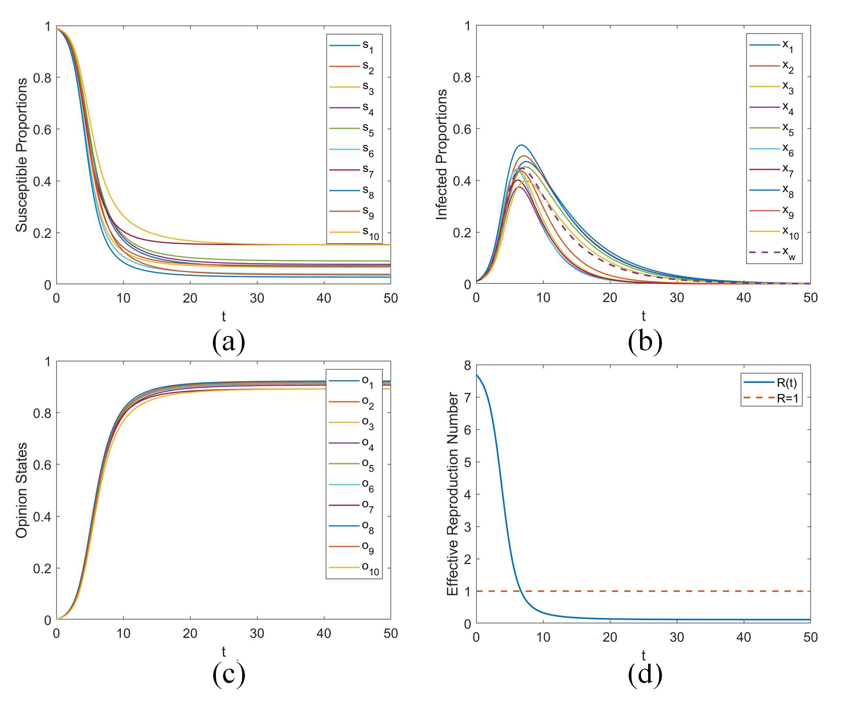
Figure 2: Typical evolution of epidemics and opinions

We set the initial condition $x(0)=0.01\times\boldsymbol{1}_{n}$, $s(0)=0.99\times\boldsymbol{1}_{n}$, and $o(0)=\boldsymbol{0}$. We also set the parameters $\beta_{\min}=0.2$, $\gamma_{\min}=0.07$, and each $\beta_{ij}$ is uniformly sampled from $[0.2,1]$. Similarly, each $\gamma_{i}$ is uniformly sampled from $[0.07,0.1]$. We apply only unit edge weights to the opinion graph in all simulations.

Fig. 2(a) shows that the proportion of the susceptible population in all communities decreases monotonically as claimed in Lemma 2, and Fig. 2(b) shows the evolution of the epidemic states, with the weighted average state $x_{w}(t)=p^{\top}(t_{p})x(t)$ $\forall t\geq 0$ being captured by the dashed line. Note that we use $p^{\top}(t_{p})$ for the entire time interval. Furthermore, the trend of the weighted average of the epidemic states follows the changes of the effective reproduction number $R_{o}(t)$ in Fig. 2(d): $x_{w}(t)=p^{\top}(t_{p})x(t)$ is increasing when $R_{o}(t)>1$; $x_{w}(t)=p^{\top}(t_{p})x(t)$ is decreasing when $R_{o}(t)<1$. Then, $x_{w}(t)=p^{\top}(t_{p})x(t)$ reaches a local peak when $R_{o}(t)=1$. Fig. 2 (a)-(d) illustrate the behavior of the system in (5a)-(5c) based on the effective reproduction number $R_{o}(t)$ and the peak infection time $t_{p}$, as we proved in Theorem 1, Corollaries 2 and 3. Additionally, Fig. 2(c) shows that, at the beginning stages of the epidemic, when no community considers the epidemic as a threat, as the susceptible population, the beliefs in the seriousness of the epidemic will increase. Meanwhile, as the susceptible population decreases and the opinion states increase, the effective reproduction number $R_{o}(t)$ decreases, which aligns with Proposition 1. As stated in Theorem 2, the states of the system converge to zero exponentially fast.

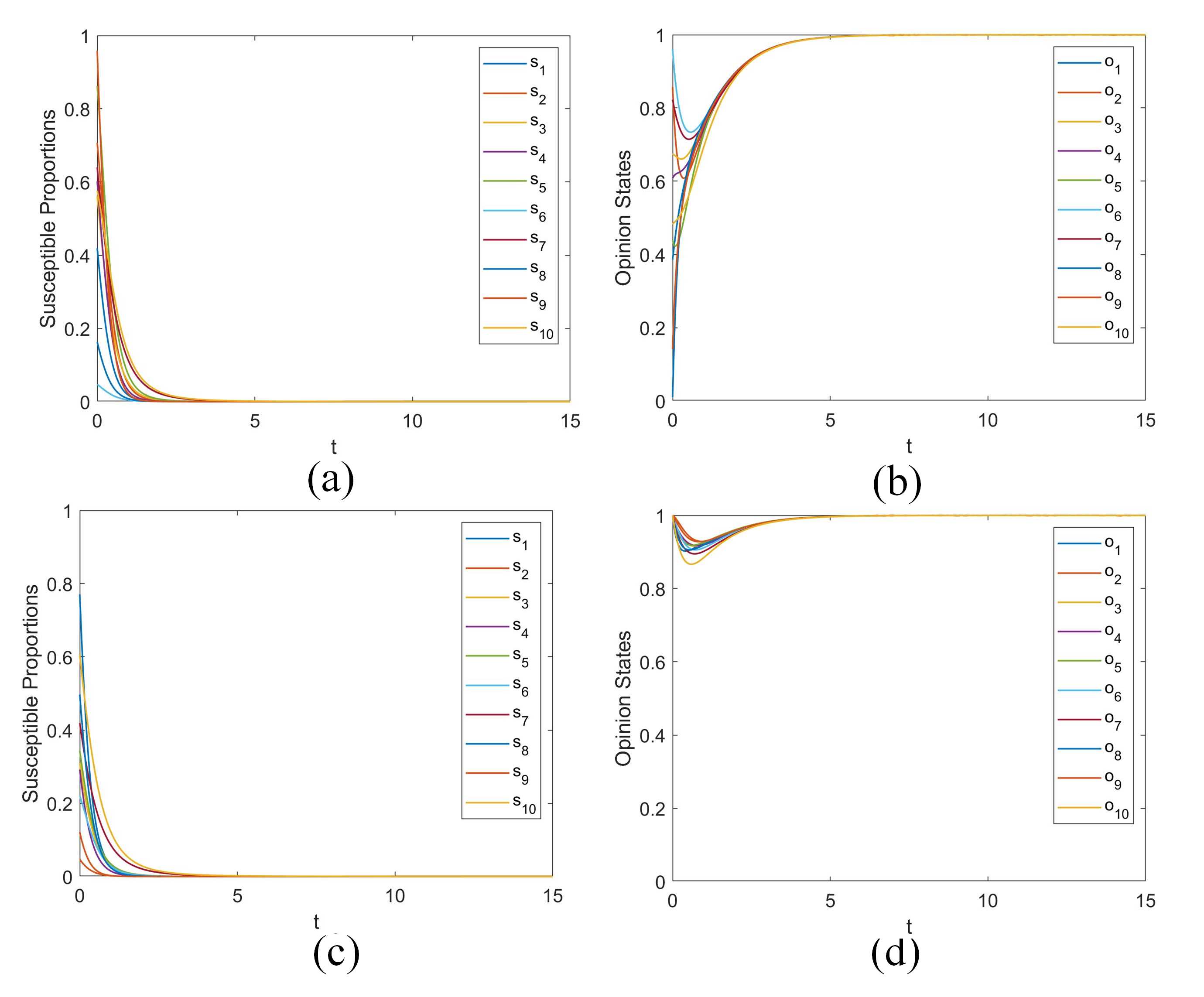
Figure 3: States convergence with wide-spread initial opinions

Next, we will show the special case where the opinions reach consensus. As mentioned in Remark 1, the opinion states will reach consensus at the equilibrium if and only if all the communities have the same infection level. We set $\beta_{\min}=0.1$ and $\gamma_{\min}=0.14$, while $\beta_{ij}$ and $\gamma_{i}$ are uniformly sampled from $[0.1,0.6]$ and $[0.14,0.30]$, respectively to generate plots in Fig. 3. In Fig. 3(a) and (c), the initial conditions of the epidemic states are uniformly sampled from $[0,1]$. In Fig. 3(b) we randomly sample the initial opinion states from $[0,1]$, and In Fig. 3(d) we set the initial opinion states as $o(0)=\boldsymbol{1}_{n}$. Both Fig. 3(a) and (c) capture the extreme case where everyone in the population becomes infected, i.e., where the susceptible states converge to $s_{e}=\boldsymbol{0}$. Therefore, based on Lemma 4, the opinion states at the equilibrium will take the form $o_{e}=\boldsymbol{1}_{n}-s_{e}=\boldsymbol{1}_{n}$, captured by Fig. 3(b) and (d). The simulations demonstrate that, when reaching agreement after the epidemic dies out, the evaluations on the seriousness of the epidemic can reflect the infection level.

Fig. 4 aims to show that the effective reproduction number $R_{o}(t)$ may not decrease monotonically, unlike the classical SIR model, as stated before. We set $\beta_{\min}=0.01$ and $\gamma_{\min}=0.05$, while $\beta_{ij}$ and $\gamma_{i}$ are uniformly sampled from $[0.01,0.4]$ and $[0.05,0.1]$, respectively. We assume initial opinions $o(0)=\boldsymbol{1}_{n}$ as shown in Fig. 4(c), and we sample the initial infected proportion for each community from $[0.3,0.6]$ randomly. In Fig. 4(d), since $R_{\min}(0)<1$, the weighted average $p^{\top}(t_{p})x(t)$ decrease at the beginning stages of the outbreak. However, the communities soon realize the epidemic is not as severe as they have evaluated as captured in Fig. 4(c). As the opinion states decrease, $R_{o}(t)$ increases, causing the weighted average $p^{\top}(t_{p})x(t)$ to increase again, captured by Fig. 4(b)-(d). In Fig. 4(d), we observe that there are two peak candidates where $R_{o}(t)=1$; we rule out the first by Theorem 1, which states that peak infection time must satisfy $R_{o}(t)>1$, for $t\in[t_{0},t_{p})$ and $R_{o}(t)<1$, for $t\in(t_{p},t_{1}]$, for $t_{p}-t_{0}>0$ and $t_{1}-t_{p}>0$ sufficiently small. However, the second point where $R_{o}(t)=1$ is a peak infection time, consistent with Fig. 4(b) and (d). Lastly, Fig. 4(d) illustrates that $R_{o}(t)$ is not monotonically decreasing, compared to the effective reproduction number in the classical SIR model [17].

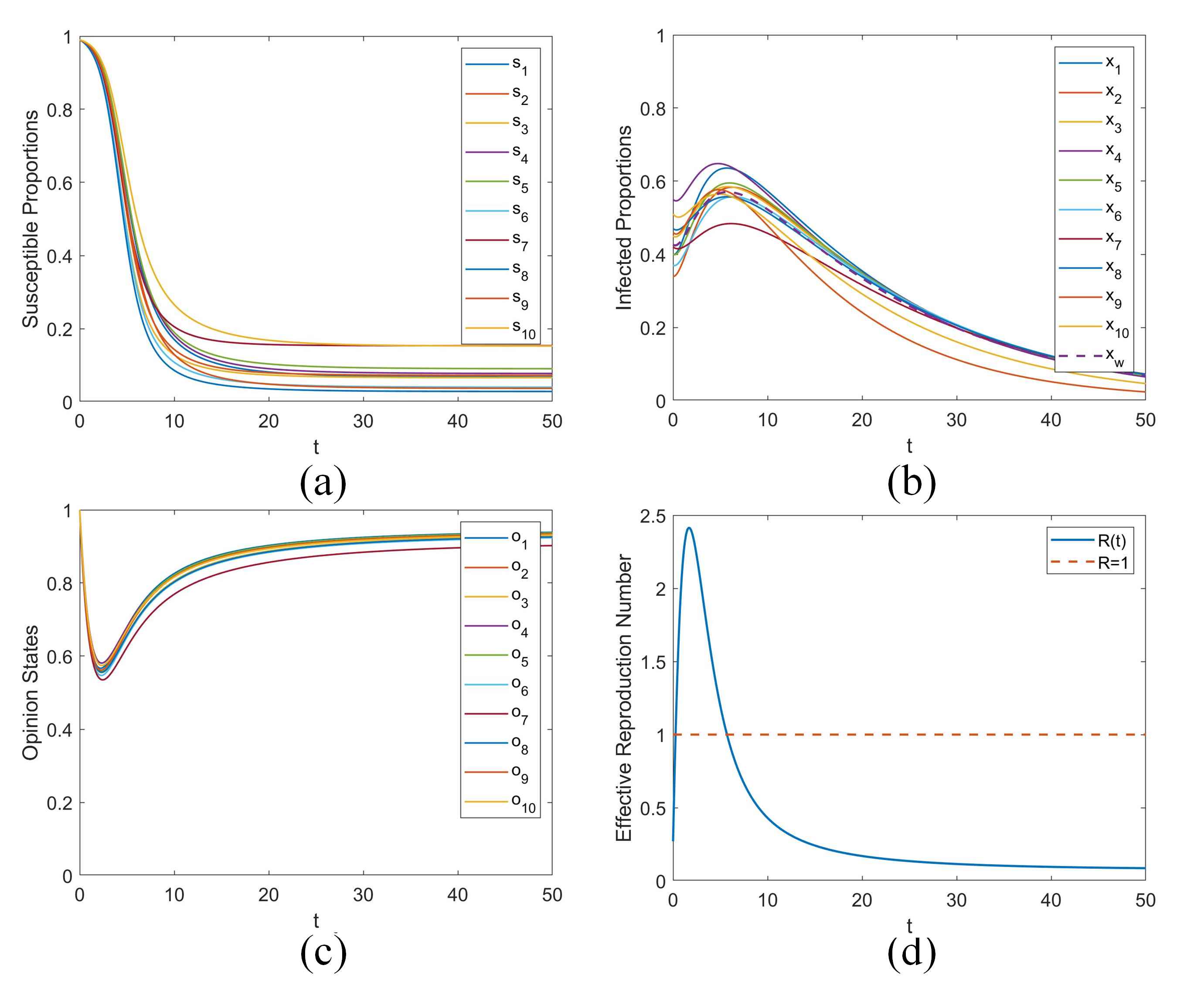
Figure 4: State dynamics with rebouncing $R_{o}(t)$

V Conclusion

In this work, we develop a networked SIR model coupled with opinion dynamics to study epidemic spreading processes over multiple communities. We define the effective reproduction number and peak infection time to characterize the transient behavior of the epidemic. We also study the convergence time to the equilibria. Additionally, we discover that the opinion states at the equilibria can reflect the infection level of each community to some degree. The current work can be further extended to study the influence of the structures of the opinion spreading networks on the behavior of the system. Another potential future research direction is to design control algorithms that influence the opinions to change the behavior of the epidemic.

References

- [1] X. Cao, “COVID-19: Immunopathology and its implications for therapy,” Nature Rev. Immunology, vol. 20, no. 5, pp. 269–270, 2020.
- [2] R. M. Anderson, H. Heesterbeek, D. Klinkenberg, and T. D. Hollingsworth, “How will country-based mitigation measures influence the course of the COVID-19 epidemic?” The Lancet, vol. 395, no. 10228, pp. 931–934, 2020.
- [3] C. Nowzari, V. M. Preciado, and G. J. Pappas, “Analysis and control of epidemics: A survey of spreading processes on complex networks,” IEEE Control Syst. Magazine, vol. 36, no. 1, pp. 26–46, 2016.
- [4] W. Mei, S. Mohagheghi, S. Zampieri, and F. Bullo, “On the dynamics of deterministic epidemic propagation over networks,” Annu. Rev. in Control, vol. 44, pp. 116–128, 2017.
- [5] K. Paarporn, C. Eksin, J. S. Weitz, and J. S. Shamma, “Networked SIS epidemics with awareness,” IEEE Trans. Comput. Soc. Syst., vol. 4, no. 3, pp. 93–103, Sept 2017.
- [6] W. Xuan, R. Ren, P. E. Paré, M. Ye, S. Ruf, and J. Liu, “On a network SIS model with opinion dynamics,” in Proc. 21st IFAC World Congress, vol. 53, no. 2, 2020, pp. 2582–2587.
- [7] A. R. Hota, J. Godbole, P. Bhariya, and P. E. Paré, “A closed-loop framework for inference, prediction and control of SIR epidemics on networks,” IEEE Trans. Network Sci. and Eng., vol. 8, no. 3, pp. 2262–2278, 2021.
- [8] J. S. Weitz, S. W. Park, C. Eksin, and J. Dushoff, “Awareness-driven behavior changes can shift the shape of epidemics away from peaks and toward plateaus, shoulders, and oscillations,” Proc. Natl. Acad. Sci., vol. 117, no. 51, pp. 32 764–32 771, 2020.
- [9] S. Bhowmick and S. Panja, “Influence of opinion dynamics to inhibit epidemic spreading over multiplex network,” IEEE Control Syst. Letters, vol. 5, no. 4, pp. 1327–1332, 2020.
- [10] K. Glanz, B. K. Rimer, and K. Viswanath, Health Behavior and Health Education: Theory, Research, and Practice. Jossey-Bass, 2008.
- [11] B. She, J. Liu, S. Sundaram, and P. E. Paré, “On a network SIS epidemic model with cooperative and antagonistic opinion dynamics,” arXiv preprint arXiv:2102.12834, 2021.
- [12] A. V. Proskurnikov and R. Tempo, “A tutorial on modeling and analysis of dynamic social networks. Part I,” Annu. Rev. in Control, vol. 43, pp. 65–79, 2017.
- [13] F. Blanchini and S. Miani, Set-Theoretic Methods in Control. Springer, 2008.
- [14] R. S. Varga, Matrix Iterative Analysis. Springer Science & Business Media, 2009, vol. 27.
- [15] J. Liu, P. E. Paré, A. Nedić, C. Tang, C. Beck, and T. Başar, “Analysis and control of a continuous-time bi-virus model,” IEEE Trans. Autom. Control, vol. 64, no. 12, pp. 4891–4906, 2019.
- [16] A. Cvetković, “Stabilizing the Metzler matrices with applications to dynamical systems,” Calcolo, vol. 57, no. 1, pp. 1–34, 2020.
- [17] P. Van den Driessche and J. Watmough, “Reproduction numbers and sub-threshold endemic equilibria for compartmental models of disease transmission,” Math. Biosci, vol. 180, no. 1-2, pp. 29–48, 2002.
- [18] H. Khalil, Nonlinear Systems. Prentice Hall, 2002.