Fast optimal trajectory generation for a tiltwing VTOL aircraft with application to urban air mobility

Abstract

We solve the minimum-thrust optimal trajectory generation problem for the transition of a tiltwing Vertical Take-Off and Landing (VTOL) aircraft using convex optimisation. The method is based on a change of differential operator that allows us to express the simplified point-mass dynamics along a prescribed path and formulate the original nonlinear problem in terms of a pair of convex programs. A case study involving the Airbus A³ Vahana VTOL aircraft is considered for forward and backward transitions. The presented approach provides a fast method to generate a safe optimal transition for a tiltwing VTOL aircraft that can further be leveraged online for control and guidance purposes.

Keywords: Convex Optimisation, Tiltwing Vertical Take-Off and Landing (VTOL) Aircraft, CVX, Urban Air Mobility.

I Introduction

The increase of congestion and pollution levels in large metropolitan areas has recently incentivized the development of sustainable and green mobility solutions. Urban Air Mobility (UAM) has the potential to address these problems by allowing air transport of goods and people [1], thus reducing the pressure on urban traffic. It has been estimated that 160,000 air taxis could be in circulation worldwide by 2050, representing a USD 90 billion market [2].

Tiltwing VTOL aircraft, with their capability to take-off and land in restricted spaces and their extended endurance, have recently received a lot of attention in a UAM context. Despite being investigated since the 1950’s [3, 4, 5], issues related to control and stability, as well as the mechanical complexity associated with the use of conventional internal combustion engines have prevented widespread adoption of this technology. However, recent advances in battery and electric motor technology, combined with the development of modern control systems architectures, has spurred a new interest for these vehicles [6]. Some recent prototypes based on tiltwing configurations are the Airbus A³ Vahana, the NASA GL-10 [7], or Rolls-Royce’s eVTOL aircraft [8].

The transition manoeuvre for a VTOL aircraft is the most critical phase of flight. Although heuristic strategies have been proposed based on smooth scheduling functions of the forward velocity or tilt angle [9], trajectory optimisation for the transition of VTOL aircraft is still an open problem as it involves determining the optimal combination of thrust and tiltwing angle to minimise an objective while meeting constraints on system states and control inputs, which requires solving large-scale nonlinear optimisation problems.

The problem of determining minimum energy speed profiles for the forward transition manoeuvre of the Airbus A³ Vahana was addressed in [10], considering various phases of flight (cruise, transition, descent). A drawback of the approach is that the transition was assumed to occur instantly, which is unrealistic for such a vehicle. In [6], the trajectory generation problem for take-off is formulated as a constrained optimisation problem and solved using NASA’s OpenMDAO framework and the SNOPT gradient-based optimiser. A case study based on the Airbus A³ Vahana tiltwing aircraft is considered, including aerodynamic models of the wing beyond stall, and the effect of propeller-wing interaction. Forward and backward optimal transition manoeuvres at constant altitude are computed in [11] for a tiltwing aircraft, considering leading-edge fluid injection active flow control and the use of a high-drag device. All of these approaches consider optimising trajectories using general purpose NLP solvers without exploiting potentially useful structures and simplifications. This approach is computationally expensive and is not generally suitable for real-time implementation.

We propose in this paper a convexification of the optimal trajectory generation problem based on a change of variables inspired by [12]. This translates the nonlinear equations of motion in the time domain into a set of linear differential equations in the space domain along a prescribed path. We thus derive an efficient method based on convex programming. Convex programming was successfully employed to solve optimisation problems related to energy management of hybrid-electric aircraft [13, 14] and spacecraft [15]. The paper is organized as follows. Section II introduces the tiltwing VTOL aircraft dynamic and aerodynamic models. Section III formulates the continuous time trajectory optimisation problem in terms of a pair of convex problems. These are discretised in Section IV and Section V discusses simulation results obtained for a case study based on the Airbus A³ Vahana. Section VI presents conclusions.

II Modeling

A simplified longitudinal point-mass model of a tiltwing VTOL aircraft equipped with propellers is developed in this section. In order to account for the effect of the propeller wake on the wing, the flow velocity downstream is augmented by the induced velocity of the propeller. The second-order dynamics of the tilting wing is also presented.

We consider a planar point-mass model of a VTOL aircraft as shown in Figure 1, whose position with respect to an inertial frame $O_{XZ}$ is given by $(x,z)$ and velocity given by

$$\dot{x}=V\cos{\gamma},\qquad\dot{z}=-V\sin{\gamma},$$

where $V$ is the aircraft velocity magnitude and $\gamma$ the flight path angle, defined as the angle of the velocity vector from horizontal. From Figure 1 the point-mass equations of motion (EOM) in polar coordinates are

$$m\dot{V} =T\cos{\alpha}-D-mg\sin{\gamma}, \quad V(t_{0}) =V_{0},$$ (1)

$$mV\dot{\gamma} =T\sin{\alpha}+L-mg\cos{\gamma}, \quad\gamma(t_{0}) =\gamma_{0},$$ (2)

where $m$ is the mass of the aircraft, $g$ the acceleration due to gravity, $T$ the thrust magnitude, $\alpha$ the angle of attack.

The dynamics of the wing are given by

$$J_{w}\ddot{i}_{w}=M,\quad i_{w}(t_{0})=i_{0},\quad\dot{i}_{w}(t_{0})=\Omega_{0},$$ (3)

where $J_{w}$ is the rotational inertia of the wing (about the $y$-axis), $M$ is the total torque delivered by the tilting actuators and $i_{w}$ is the tiltwing angle such that

$$i_{w}+\theta=\alpha+\gamma.$$

Here $\theta$ is the pitch angle, defined as the angle of the fuselage axis from horizontal. For passenger comfort, $\theta$ is regulated via the elevator to track a constant reference $\theta^{*}=0$.

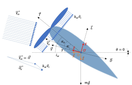
Figure 1: Force and velocity definitions for a VTOL aircraft

From momentum theory, the propeller generates an induced speed $v_{i}$ such that

$$T=\rho An(V\cos{\alpha}+v_{i})(k_{w}v_{i}),$$

where $\rho$ is the air density, $A$ the rotor disk area, $n$ the number of propellers, and $k_{w}\approx 2$. The effective velocity $V_{e}$ and effective angle of attack $\alpha_{e}$ seen by the wing are given by

$$V_{e}\cos{\alpha_{e}} =V\cos{\alpha}+k_{w}v_{i},$$

$$V_{e}\sin{\alpha_{e}} =V\sin{\alpha},$$

$$V_{e}^{2}=V^{2}+\frac{2T}{\rho An}.$$

The total lift and drag are modeled as the weighted sum of the blown and unblown counterparts

$$D =(1-\mu)\tfrac{1}{2}\rho S(a_{2}\alpha^{2}+a_{1}\alpha+a_{0})V^{2}$$

$$\quad+\mu\tfrac{1}{2}\rho S(a_{2}\alpha_{e}^{2}+a_{1}\alpha_{e}+a_{0})V_{e}^{2}$$

$$\approx(1-\mu)\tfrac{1}{2}\rho S(a_{1}\alpha+a_{0})V^{2}+\mu\tfrac{1}{2}\rho S(a_{1}\alpha_{e}+a_{0})V_{e}^{2},$$

$$L =(1-\mu)\tfrac{1}{2}\rho S(b_{1}\alpha+b_{0})V^{2}+\mu\tfrac{1}{2}\rho S(b_{1}\alpha_{e}+b_{0})V_{e}^{2}.$$

Here $S$ is the wing area, $\mu=2Rn/l$ is the blown-unblown ratio, $R$ is the radius of the rotor disk, $l$ is the wingspan, $a_{0},a_{1},a_{2}$ and $b_{0},b_{1}$ are constant parameters and $\alpha,\alpha_{e}\ll 1$ is assumed so that terms involving $\alpha^{2},\alpha_{e}^{2}$ are negligible. The following input and state constraints also apply

$$0\leq T\leq\overline{T},\quad 0\leq V\leq\overline{V},$$

$$V(t_{0})=V_{0}\text{ and }V(t_{f})=V_{f},$$

$$\underline{a}\leq\dot{V}\leq\overline{a},\quad\underline{M}\leq M\leq\overline{M}.$$

This paper considers how to optimise the transition between powered lift and cruise flight modes. Minimising thrust is a natural choice as a proxy for minimising energy consumption, suggesting the following objective function

$$J=\int_{t_{0}}^{t_{f}}\left(T/\overline{T}\right)^{2}\mathrm{d}t.$$ (4)

The optimisation problem consists of minimising (4) while satisfying dynamical constraints, input and state constraints.

III Convex formulation

The aircraft dynamics derived in Section II contain nonlinearities that make the trajectory optimisation problem nonconvex. However, a change of variables (motivated by [12]) considerably simplifies the structure of this problem and allows us to formulate the problem in terms of two convex programs. If we assume that a path $(x(s),z(s))$ parameterised by the curvilinear abscissa $s$ is already known a priori (which is usually the case in a UAM context where flight corridors are prescribed) we can introduce via the chain rule the following change of differential operator,

$$\frac{\mathrm{d}}{\mathrm{d}t}=V\frac{\mathrm{d}}{\mathrm{d}s}.$$ (5)

Denoting $\tfrac{\mathrm{d}\,\cdot}{\mathrm{d}s}=\cdot^{\prime}$, the EOM in (1) and (2) are equivalent to

$$mVV^{\prime} =T\cos{\alpha}-(1-\mu)\frac{1}{2}\rho S(a_{1}\alpha+a_{0})V^{2}$$

$$\quad-\mu\frac{1}{2}\rho S(a_{1}\alpha_{e}+a_{0})\Bigl{(}V^{2}+\frac{2T}{\rho An}\Bigr{)}-mg\sin{\gamma^{*}},$$

$$mV^{2}\gamma^{*\prime} =T\sin{\alpha}+(1-\mu)\frac{1}{2}\rho S(b_{1}\alpha+b_{0})V^{2}$$

$$\quad+\mu\frac{1}{2}\rho S(b_{1}\alpha_{e}+b_{0})\Bigl{(}V^{2}+\frac{2T}{\rho An}\Bigr{)}-mg\cos{\gamma^{*}},$$

where $\gamma^{*}$ is known a priori from the path. Specifically, since $\mathrm{d}x=V\cos{\gamma}\,\mathrm{d}t$ and $\mathrm{d}z=-V\sin{\gamma}\,\mathrm{d}t$, the flight path angle can be expressed in terms of the path variables as

$$\tan{\gamma^{*}}=-\frac{\mathrm{d}z}{\mathrm{d}x}.$$

Defining new model states $E=V^{2}$ and $a=VV^{\prime}$, so that

$$E^{\prime}=2a,$$ (6)

the EOM reduce to

$$ma=T\cos{\alpha}-(1-\mu)\frac{1}{2}\rho S\left(a_{1}\alpha+a_{0}\right)E$$

$$\quad-\mu\frac{1}{2}\rho S\left(a_{1}\alpha_{e}+a_{0}\right)\left(E+\frac{2T}{\rho An}\right)-mg\sin{\gamma^{*}},$$ (7)

$$mE\gamma^{*\prime}=T\sin{\alpha}+(1-\mu)\frac{1}{2}\rho S\left(b_{1}\alpha+b_{0}\right)E$$

$$\quad+\mu\frac{1}{2}\rho S\left(b_{1}\alpha_{e}+b_{0}\right)\left(E+\frac{2T}{\rho An}\right)-mg\cos{\gamma^{*}}.$$ (8)

Let $\lambda=a_{1}/b_{1}$, then the linear combination (III) $+$ $\lambda$(III) yields

$$\!\!\!\!\!ma+\underbrace{(\lambda m\gamma^{*\prime}+\frac{1}{2}\rho S(a_{0}-\lambda b_{0}))}_{c(\gamma^{*\prime})}E+\underbrace{mg(\sin{\gamma^{*}}+\lambda\cos{\gamma^{*}})}_{d(\gamma^{*})}\\ =\underbrace{T\cos{\alpha}+\lambda T\sin{\alpha}-\mu S^{\star}(a_{0}-\lambda b_{0})T}_{\tau},$$ (9)

where $S^{\star}=\frac{S}{AN}$ and $\tau$ is a virtual input defined by

$$\tau=T\cos{\alpha}+\lambda T\sin{\alpha}-\mu S^{\star}(a_{0}-\lambda b_{0})T.$$ (10)

Since $\gamma^{*}$ is prescribed by the path, (9) and (6) form a differential-algebraic system of linear equations and can thus be included as part of a convex program.

The constraints on the state variables can be rewritten as

$$0\leq E\leq\overline{V}^{2},\quad\underline{a}\leq a\leq\overline{a},$$

$$E(s_{0})=V_{0}^{2}\text{ and }E(s_{f})=V_{f}^{2}.$$

The thrust constraint $0\leq T\leq\overline{T}$ cannot be expressed exactly as a function of $\tau$ only. However, assuming that $\alpha\ll 1$, and noting that $\lambda\ll 1$, and $S^{\star}(a_{0}-\lambda b_{0})\ll 1$ we have $\tau\approx T$ and $0\leq T\leq\overline{T}$ is therefore approximately equivalent to

$$0\leq\tau\leq\overline{T}.$$

Finally the minimum thrust criterion in (4) can be approximated by a convex objective function under these conditions, since $\tau$ is then a good proxy for the thrust. By the change of differential operator in (5) we obtain

$$J=\int_{s_{0}}^{s_{f}}\frac{(\tau/\overline{T})^{2}}{\sqrt{E}}\,\mathrm{d}s.$$

We can thus state the following convex optimisation problem for a given path (i.e. given $\gamma$ and $\gamma^{\prime}$) as follows

$$\mathcal{P}_{1}:\min_{\begin{subarray}{c}\tau,\,E,\,a\end{subarray}} \int_{s_{0}}^{s_{f}}\frac{(\tau/\overline{T})^{2}}{\sqrt{E}}\,\mathrm{d}s,$$

s.t. $$ma+c(\gamma^{*\prime})E+d(\gamma^{*})=\tau,$$

$$E^{\prime}=2a,$$

$$0\leq\tau\leq\overline{T},\ \underline{a}\leq a\leq\overline{a},$$

$$0\leq E\leq\overline{V}^{2},\ E(s_{0})=V_{0}^{2},\ E(s_{f})=V_{f}^{2}.$$

Solving $\mathcal{P}_{1}$ yields the optimal velocity along the path and a proxy for the optimal thrust for sufficiently small values of the angle of attack ($\tau\approx T$). However, a tiltwing angle profile that meets the dynamical constraints and follows the desired path with $\gamma\approx\gamma^{*}$ must also be computed. To achieve this we use the solution of $\mathcal{P}_{1}$ to define a new optimisation problem with variables $\gamma$, $\alpha$, $i_{w}$, and $M$ satisfying the constraints

$$J_{w}(i_{w}^{\prime}a+i_{w}^{\prime\prime}E)=M,$$ (11)

$$\underline{M}\leq M\leq\overline{M},$$

$$i_{w}=\alpha+\gamma,$$

$$mE\gamma^{\prime}=\tau\sin{\alpha}+(1-\mu)\frac{1}{2}\rho S(b_{1}\alpha+b_{0})E-mg\cos{\gamma}$$

$$+\mu\frac{1}{2}\rho S\biggl{[}b_{1}\arcsin\biggl{(}\frac{\sqrt{E}\sin{\alpha}}{\sqrt{E+\smash{\frac{2\tau}{\rho An}}\rule{0.0pt}{8.5pt}}}\biggr{)}+b_{0}\biggr{]}\Bigl{(}E+\frac{2\tau}{\rho An}\Bigr{)},$$ (12)

in which the objective is to minimise the cost function

$$J_{\gamma}=\int_{s_{0}}^{s_{f}}\frac{(\gamma-\gamma^{*})^{2}}{\sqrt{E}}\mathrm{d}s.$$ (13)

Note that to obtain (11) from (3), we have used the result $\frac{\mathrm{d^{2}}}{\mathrm{d}t^{2}}=V\frac{\mathrm{d}}{\mathrm{d}s}\left(V\frac{\mathrm{d}}{\mathrm{d}s}\right)=a\frac{\mathrm{d}}{\mathrm{d}s}+E\frac{\mathrm{d^{2}}}{\mathrm{d}s^{2}}$ inferred from the change of differential operator in (5). To convexify the problem and to support the small angle approximation $\alpha,\alpha_{e}\ll 1$ used in the derivation of the EOM, we enforce bounds on $\alpha$ by imposing constraints $\underline{\alpha}~{}\leq~{}\alpha~{}\leq~{}\overline{\alpha}$, for sufficiently small $\underline{\alpha}$, $\overline{\alpha}$, chosen such that the wing is unstalled, and linear relationship with lift coefficient applies. This allows the dependence of (12) on $\alpha$ to be linearised

$$mE\gamma^{\prime}=\underbrace{\biggl{(}\tau+(1\!-\!\mu)\frac{1}{2}\rho Sb_{1}E+\mu\frac{1}{2}\rho Sb_{1}\sqrt{E^{2}+\tfrac{2\tau E}{\rho An}}\biggr{)}}_{p(E,\tau)}\alpha\\ +\underbrace{(1-\mu)\frac{1}{2}\rho Sb_{0}E+\mu\frac{1}{2}\rho Sb_{0}\Bigl{(}E+\frac{2\tau}{\rho An}\Bigr{)}}_{q(E,\tau)}-mg\cos{\gamma}.$$ (14)

Although $p(E,\tau)$ and $q(E,\tau)$ are determined by the solution of $\mathcal{P}_{1}$, (14) is nonconvex since the last term is nonlinear in the decision variable $\gamma$. However, (14) can be omitted from the problem if the objective function (13) is augmented

$$J^{a}_{\gamma}=\int_{s_{0}}^{s_{f}}\frac{(\gamma-\gamma^{*})^{2}}{\sqrt{E}}+\frac{(p\alpha+q-mE\gamma^{\prime}-mg\cos{\gamma^{*}})^{2}}{(mg)^{2}\sqrt{E}}\mathrm{d}s.$$ (15)

This objective attempts to minimise the error between the guessed and actual flight path angles while enforcing (14) in the sense that, if a feasible solution exists satisfying both $\gamma=\gamma^{\ast}$ and (14), then the optimal solution must satisfy (14).

We thus state the following optimisation problem, with $\tau$, $E$ and $a$ prescribed from problem $\mathcal{P}_{1}$

$$\mathcal{P}_{2}:\min_{\begin{subarray}{c}\alpha,\,\gamma,\,i_{w},\,M\end{subarray}} \int_{s_{0}}^{s_{f}}\frac{(\gamma-\gamma^{*})^{2}}{\sqrt{E}}\mathrm{d}s$$

$$+\int_{s_{0}}^{s_{f}}\frac{(p\alpha+q-mE\gamma^{\prime}-mg\cos{\gamma^{*}})^{2}}{(mg)^{2}\sqrt{E}}\mathrm{d}s$$

s.t. $$J_{w}(i_{w}^{\prime}a+i_{w}^{\prime\prime}E)=M,\ i_{w}(s_{0})=i_{0},$$

$$i_{w}^{\prime}(s_{0})\sqrt{E(s_{0})}=\Omega_{0},$$

$$i_{w}=\alpha+\gamma,$$

$$\underline{M}\leq M\leq\overline{M},\ \underline{\alpha}\leq\alpha\leq\overline{\alpha}$$

$$\underline{\gamma}\leq\gamma\leq\overline{\gamma},\ \underline{i_{w}}\leq i_{w}\leq\overline{i_{w}}.$$

It should be emphasized that $\mathcal{P}_{2}$ may admit solutions that allow $\gamma$ to divert from the guessed flight path angle $\gamma^{*}$. This occurs for example when the bounds on angle of attack do not allow the desired path to be followed (see e.g. Section V, scenario 2). In this case, problems $\mathcal{P}_{1}$ and $\mathcal{P}_{2}$ can be rerun sequentially after reinitializing with the newly obtained path ($\gamma^{*}\leftarrow\gamma$). This process can be repeated iteratively until $\gamma$ is sufficiently close to $\gamma^{*}$. Although we do not provide theoretical guarantees of convergence for this case, we note that the objective value has decreased by orders of magnitude after several iterations, as illustrated in Section V.

Only one EOM (III) was needed to constrain the variables of problem $\mathcal{P}_{2}$ since the EOM (III) can be enforced a posteriori by choosing $T$ so that equation (10) is satisfied

$$T=\frac{\tau}{\cos{\alpha}+\lambda\sin{\alpha}-\mu S^{\star}(a_{0}-\lambda b_{0})}.$$

This guarantees that the solution satisfies both EOM within the required accuracy, since problem $\mathcal{P}_{1}$ includes a linear combination of (III) and (III), and problem $\mathcal{P}_{2}$ enforces (III).

Given an optimal set of inputs and states as functions of the independent variable $s$, the final step is to convert back to time domain. This can be done by reversing the change of differential operator in equation (5) and integrating

$$t(\xi)=\int_{s_{0}}^{\xi}\frac{\mathrm{d}s}{V(s)}.$$

IV Discrete convex optimisation

The decision variables in $\mathcal{P}_{1}$ and $\mathcal{P}_{2}$ are functions defined on the interval $[s_{0},s_{f}]$. To obtain computationally tractable problems, we consider $N+1$ discretisation points $\{s_{0},s_{1},\ldots,s_{N}\}$ of the path, with spacing $\delta_{k}=s_{k+1}-s_{k}$, $k=0,\ldots,N-1$ ($N$ steps). The notation $\{u_{0},\ldots,u_{N}\}$ is used for the sequence of the discrete values of a continuous variable $u$ evaluated at the discretisation points of the mesh, where $u_{k}=u(s_{k})$, $\forall k\in\{0,\ldots,N\}$.

Assuming a path $s_{k}\rightarrow(x_{k},z_{k})$, the prescribed flight path angle and rate are discretised as follows

$$\gamma_{k}^{*} =\arctan\Bigl{(}-\frac{z_{k+1}-z_{k}}{x_{k+1}-x_{k}}\Bigr{)},\quad k\in\{0,\ldots,N-1\},$$ (16)

$$\gamma_{k}^{*\prime} =\begin{cases}(\gamma_{k+1}^{*}-\gamma_{k}^{*})/{\delta_{k}},&k\in\{0,\ldots,N-2\},\\ \gamma_{N-2}^{*\prime},&k=N-1.\end{cases}$$ (17)

The resulting discrete time versions of $\mathcal{P}_{1}$ and $\mathcal{P}_{2}$ are

$$\mathcal{P}_{1}^{\dagger}:\min_{\begin{subarray}{c}\tau,\,E,\,a\end{subarray}} \sum_{k=0}^{N-1}\frac{(\tau_{k}/\overline{T})^{2}}{\sqrt{E_{k}}}\,\delta_{k},$$

s.t. $$ma_{k}+c(\gamma_{k}^{*\prime})E_{k}+d(\gamma_{k}^{*})=\tau_{k},$$

$$E_{k+1}=E_{k}+2a_{k}\delta_{k},$$

$$0\leq\tau_{k}\leq\overline{T},\quad\underline{a}\leq a_{k}\leq\overline{a},$$

$$0\leq E_{k}\leq\overline{V}^{2},\quad E_{0}=V_{0}^{2},\quad E_{N}=V_{f}^{2},$$

$$\mathcal{P}_{2}^{\dagger}:\min_{\begin{subarray}{c}\alpha,\,\gamma,\,\theta,\\ i_{w},\,\zeta,\,M\end{subarray}} \sum_{k=0}^{N-1}\frac{(\gamma_{k}-\gamma_{k}^{*})^{2}}{\sqrt{E_{k}}}\delta_{k}$$

$$+\sum_{k=0}^{N-1}\frac{(p\alpha_{k}+q-mE_{k}\Psi_{k}-mg\cos{\gamma_{k}^{*}})^{2}}{(mg)^{2}\sqrt{E_{k}}}\delta_{k},$$

s.t. $$\gamma_{k+1}=\gamma_{k}+\Psi_{k}\delta_{k},$$

$$i_{w,k}=\alpha_{k}+\gamma_{k},$$

$$i_{w,k+1}=i_{w,k}+\zeta_{k}\delta_{k},\quad i_{w,0}=i_{0},$$

$$\zeta_{k+1}=\zeta_{k}\Bigl{(}1-\frac{a_{k}\delta_{k}}{E_{k}}\Bigr{)}+\frac{M_{k}\delta_{k}}{J_{w}{E_{k}}},$$

$$\zeta_{0}\sqrt{E}_{0}=\Omega_{0},$$

$$\underline{M}\leq M_{k}\leq\overline{M},\quad\underline{\alpha}\leq\alpha_{k}\leq\overline{\alpha},$$

$$\underline{\gamma}\leq\gamma_{k}\leq\overline{\gamma},\quad\underline{i_{w}}\leq i_{w,k}\leq\overline{i_{w}}.$$

Once $\mathcal{P}_{1}^{\dagger}$ and $\mathcal{P}_{2}^{\dagger}$ have been solved, we check whether $|\gamma_{k}^{*}-\gamma_{k}|\leq\epsilon$ $\forall k\in\{0,\ldots,N\}$, where $\epsilon$ is a specified tolerance. If this condition is not met, the problem is reinitialized with the updated flight path angle and rate $\gamma^{*}_{k}\leftarrow\gamma_{k}$, $\gamma^{*\prime}_{k}\leftarrow\gamma_{k}^{\prime}$. and $\mathcal{P}_{1}^{\dagger}$ and $\mathcal{P}_{2}^{\dagger}$ are solved again. When the solution tolerance is met (or the maximum number of iterations is exceeded) the problem is considered solved and the input and state variables are reconstructed using

$$T_{k} =\frac{\tau_{k}}{\cos{\alpha_{k}}+\lambda\sin{\alpha_{k}}-\mu S^{\star}(a_{0}-\lambda b_{0})},\quad V_{k} =\sqrt{E_{k}},$$

and the time $t_{k}$ associated with each discretisation point is computed, allowing solutions to be expressed as time series

$$t_{k}=\sum_{j=0}^{k-1}\frac{\delta_{j}}{V_{j}}.$$

The procedure is summarised in Algorithm 1.

Compute $\gamma^{*}$, $\gamma^{*\prime}$ using (16), (17) and initialise: $\gamma\leftarrow\gamma^{*}$, $\gamma^{\prime}\leftarrow\gamma^{*\prime}$, $\gamma^{*}\leftarrow\infty$, $j\leftarrow 0$

while $\displaystyle\max_{k\in\{0,\ldots,N\}}|\gamma_{k}^{*}-\gamma_{k}|>\epsilon$ $\&$ $j<$ MaxIters do

       $\gamma^{*}\leftarrow\gamma$, $\gamma^{*\prime}\leftarrow\gamma^{\prime}$

       Solve problem $\mathcal{P}_{1}^{\dagger}$ and problem $\mathcal{P}_{2}^{\dagger}$

       $j\leftarrow j+1$

end while

for $k\leftarrow 0$ to $N$ do

       $T_{k}\leftarrow\frac{\tau_{k}}{\cos{\alpha_{k}}+\lambda\sin{\alpha_{k}}-\mu S^{\star}(a_{0}-\lambda b_{0})}$

       $V_{k}\leftarrow\sqrt{E_{k}}$

       $t_{k}\leftarrow\sum_{j=0}^{k-1}\frac{\delta_{j}}{V_{j}}$

end for

Algorithm 1 Convex trajectory optimisation

V Results

We consider a case study based on the Airbus A³ Vahana. The aircraft parameters are reported in Table I. We run Algorithm 1 using the convex programming software package CVX [16] with the solver Mosek [17] to compute the optimal trajectory for 3 different transition manoeuvres, with boundary conditions given in Table II.

The first scenario is a forward smooth transition where the flight path angle varies slowly from $75^{\circ}$ to a value close to zero, as illustrated in Figure 2. As the aircraft transitions from powered lift to cruise, the velocity magnitude increases and the thrust decreases, illustrating the change in lift generation from propellers to wing. The angle of attack remains small over the transition as it occurs smoothly.

The second scenario is a constant altitude forward transition. This manoeuvre is more abrupt and would require a zero flight path angle throughout, thus exceeding the bounds on $\alpha$ at the beginning when the wing is tilted vertically. Solving problem $\mathcal{P}_{2}^{\dagger}$ with constraints on $\alpha$ initially yields an optimal $\gamma$ profile that differs from the anticipated zero flight path angle. Reinitializing the problem with the computed flight path angle ($\gamma^{*}\leftarrow\gamma$) and iterating until a satisfactory match between $\gamma$ and $\gamma^{*}$ is achieved results in convergence illustrated empirically in Figure 3. The solution thus obtained is shown in Figure 4. Since the flight path angle is not identically zero (as would be required for a constant altitude transition) the manoeuvre is characterised by an initial increase in altitude and overshoot of about 30 m. This is a consequence of limiting the angle of attack. More abrupt transitions with smaller altitude variations are possible, but this requires stalling the wing and operating in flight envelopes for which our approximations are not valid.

The third scenario is a backward transition with an increase in altitude (Figure 5). This is characterised by an initial decrease in velocity magnitude and increase in thrust. The strict bounds on angle of attack necessitate an increase in altitude of about 100 m. A backward transition at constant altitude would require stalling the wing, which is prohibited in the present formulation, illustrating a limitation of our approach. To achieve the backward transition, a high-drag device or flaps are needed to provide braking forces. This can be modelled by adding a constant term $\delta$ to $c(\gamma^{*\prime})$ in problem $\mathcal{P}_{1}^{\dagger}$ when simulating the backward transition.

The time-complexity of the proposed algorithm in scenario 1 is shown in Figure 6. The time to completion as a function of problem size (number of discretisation points) is asymptotically quadratic, implying excellent scalability. In particular, for $N<1500$, the time to completion is of the order of seconds. A real-time solution is thus possible using modest computational resources. This is in stark contrast to the complexity of generic NLP approaches [11]. Moreover, as shown in [14], the time complexity for this type of problem can be reduced significantly with first-order solvers, paving the way for fast real-time implementations.

Parameter	Symbol	Value	Units
Mass	$m$	$752.2$	$\mathrm{k}\mathrm{g}$
Gravity acceleration	$g$	$9.81$	$\mathrm{m}\,\mathrm{s}^{-2}$
Wing area	$S$	$8.93$	$\mathrm{m}^{2}$
Disk area	$A$	$2.83$	$\mathrm{m}^{2}$
Blown-unblown ratio	$\mu$	$0.73$	$\mathrm{-}$
Wing inertia	$J_{w}$	$1100$	$\mathrm{k}\mathrm{g}\,\mathrm{m}^{2}$
Density of air	$\rho$	$1.225$	$\mathrm{k}\mathrm{g}\,\mathrm{m}^{-3}$
Lift coefficients	$b_{0},b_{1}$	$0.43,0.11$	$\mathrm{-}$, $\mathrm{d}\mathrm{e}\mathrm{g}^{-1}$
Drag coefficients	$a_{0},a_{1}$	$0.029,0.004$	$\mathrm{-}$, $\mathrm{d}\mathrm{e}\mathrm{g}^{-1}$
Maximum thrust	$\overline{T}$	$8855$	$\mathrm{N}$
Angle of attack range	$\left[\underline{\alpha},\overline{\alpha}\right]$	$\left[-20,20\right]$	$\mathrm{d}\mathrm{e}\mathrm{g}$
Flight path angle range	$\left[\underline{\gamma},\overline{\gamma}\right]$	$\left[-90,90\right]$	$\mathrm{d}\mathrm{e}\mathrm{g}$
Tiltwing angle range	$\left[\underline{i}_{w},\overline{i}_{w}\right]$	$\left[0,100\right]$	$\mathrm{d}\mathrm{e}\mathrm{g}$
Acceleration range	$\left[\underline{a},\overline{a}\right]$	$\left[-0.3g,0.3g\right]$	$\mathrm{m}\,\mathrm{s}^{-2}$
Velocity range	$\left[\underline{V},\overline{V}\right]$	$\left[0,40\right]$	$\mathrm{m}\mathrm{/}\mathrm{s}$
Momentum range	$\left[\underline{M},\overline{M}\right]$	$\left[-50;50\right]$	$\mathrm{N}\,\mathrm{m}$
Number of propellers	$n$	$4$	$\mathrm{-}$
Discretisation points	$N$	$1500$	$\mathrm{-}$

TABLE I: Model parameters derived from A³ Vahana

Parameter	Symbol	Value	Units
[rgb]0.753,0.753,0.753Forward transition
Velocity	$\left\{V_{0};V_{f}\right\}$	$\left\{0.5;40\right\}$	$\mathrm{m}\mathrm{/}\mathrm{s}$
Tiltwing angle	$i_{0}$	$75$	$\mathrm{d}\mathrm{e}\mathrm{g}$
Tiltwing angle rate	$\Omega_{0}$	$0$	$\mathrm{d}\mathrm{e}\mathrm{g}\mathrm{/}\mathrm{s}$
Flight path angle	$\gamma_{0}$	$75$	$\mathrm{d}\mathrm{e}\mathrm{g}$
[rgb]0.753,0.753,0.753Backward transition
Velocity	$\left\{V_{0};V_{f}\right\}$	$\left\{40;0.1\right\}$	$\mathrm{m}\mathrm{/}\mathrm{s}$
Tiltwing angle	$\left\{i_{0};i_{f}\right\}$	$\left\{0;75\right\}$	$\mathrm{d}\mathrm{e}\mathrm{g}$
Tiltwing angle rate	$\Omega_{0}$	$0$	$\mathrm{d}\mathrm{e}\mathrm{g}\mathrm{/}\mathrm{s}$
Flight path angle	$\gamma_{0}$	$1.6$	$\mathrm{d}\mathrm{e}\mathrm{g}$

TABLE II: Boundary conditions for transitions

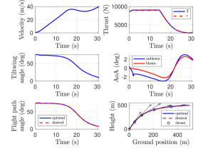
Figure 2: Forward transition (scenario 1)

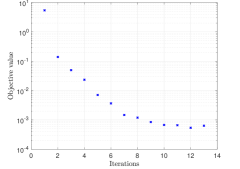
Figure 3: Convergence of objective value for $\mathcal{P}_{2}^{\dagger}$ (scenario 2)

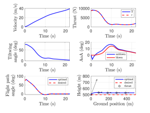
Figure 4: Forward transition (scenario 2)

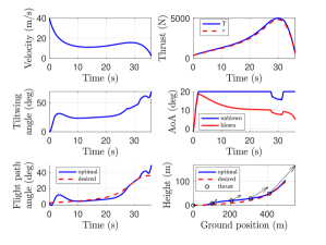
Figure 5: Backward transition (scenario 3)

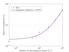
Figure 6: Time to completion as a function of problem size

VI Conclusions

A convex programming formulation of the minimum thrust transition problem for a tiltwing VTOL aircraft with propeller-wing interaction was proposed and solved for various transition scenarios. The approach can compute an optimal trajectory within seconds for large numbers of discretisation points and is particularly efficient at computing smooth transitions. A potential limitation of the approach is its reliance on small angles of attack, which may restrict the range of achievable manoeuvres. In particular, more abrupt manoeuvres with larger angles of attack are prohibited. Another drawback is that, for the case in which the initial guess of flight path angle is infeasible, the evidence for the convergence of the proposed iteration is empirical rather than theoretical. Future work will address these two issues using techniques from robust MPC theory. A further extension to this work is to develop a first-order solver for online trajectory generation.

References

- [1] McKinsey, “Study on the societal acceptance of Urban Air Mobility in Europe,” European Union Aviation Safety Agency (EASA), 2021.
- [2] M. Hader, S. Baur, S. Kopera, T. Schönberg, and J.-P. Hasenberg, “Urban air mobility, USD 90 billion of potential: how to capture a share of the passenger drone market,” Roland Berger, 2020.
- [3] R. E. Kuhn, “Semiempirical procedure for estimating lift and drag characteristics of propeller-wing-flap configurations for vertical-and short-take-off-and-landing airplanes,” NASA Memorandum, 1959.
- [4] C. R. Hargraves, “An analytical study of the longitudinal dynamics of a tilt-wing VTOL,” tech. rep., Princeton University, 1961.
- [5] B. W. McCormick, Aerodynamics of V/STOL flight. Academic Press, London, 1967.
- [6] S. S. Chauhan and J. R. Martins, “Tilt-wing eVTOL takeoff trajectory optimization,” Journal of Aircraft, pp. 1–20, 2019.
- [7] P. M. Rothhaar, P. C. Murphy, B. J. Bacon, I. M. Gregory, J. A. Grauer, R. C. Busan, and M. A. Croom, “NASA langley distributed propulsion VTOL tiltwing aircraft testing, modeling, simulation, control, and flight test development,” in 14th AIAA aviation technology, integration, and operations conference, p. 2999, 2014.
- [8] R. J. Higgins, G. N. Barakos, S. Shahpar, and I. Tristanto, “An aeroacoustic investigation of a tiltwing eVTOL concept aircraft,” in AIAA AVIATION 2020 FORUM, p. 2684, 2020.
- [9] R. Chiappinelli, M. Cohen, M. Doff-Sotta, M. Nahon, J. R. Forbes, and J. Apkarian, “Modeling and control of a passively-coupled tilt-rotor vertical takeoff and landing aircraft,” in 2019 International Conference on Robotics and Automation (ICRA), pp. 4141–4147, IEEE, 2019.
- [10] P. Pradeep and P. Wei, “Energy optimal speed profile for arrival of tandem tilt-wing eVTOL aircraft with RTA constraint,” in IEEE CSAA Guidance, Navigation and Control Conference, 2018.
- [11] L. Panish and M. Bacic, “Transition trajectory optimization for a tiltwing VTOL aircraft with leading-edge fluid injection active flow control,” AIAA Scitech 2022 San Diego, 2022.
- [12] J. E. Bobrow, S. Dubowsky, and J. S. Gibson, “Time-optimal control of robotic manipulators along specified paths,” The international journal of robotics research, vol. 4, no. 3, pp. 3–17, 1985.
- [13] M. Doff-Sotta, M. Cannon, and M. Bacic, “Optimal energy management for hybrid electric aircraft,” IFAC-PapersOnLine, vol. 53, no. 2, pp. 6043–6049, 2020.
- [14] M. Doff-Sotta, M. Cannon, and M. Bacic, “Predictive energy management for hybrid electric aircraft propulsion systems,” IEEE Transactions on Control Systems Technology (under review), 2021.
- [15] M. Doff-Sotta, M. Cannon, and J. Forbes, “Spacecraft energy management using convex optimisation,” under review, 2021.
- [16] M. Grant and S. Boyd, “CVX: Matlab software for disciplined convex programming, version 2.1.” http://cvxr.com/cvx, Mar. 2014.
- [17] M. ApS, Introducing the MOSEK Optimization Suite 9.3.6, 2021.