Spreading of fake news, competence, and learning: kinetic modeling and numerical approximation

Abstract

The rise of social networks as the primary means of communication in almost every country in the world has simultaneously triggered an increase in the amount of fake news circulating online. This fact became particularly evident during the 2016 U.S. political elections and even more so with the advent of the COVID-19 pandemic. Several research studies have shown how the effects of fake news dissemination can be mitigated by promoting greater competence through lifelong learning and discussion communities, and generally rigorous training in the scientific method and broad interdisciplinary education. The urgent need for models that can describe the growing infodemic of fake news has been highlighted by the current pandemic. The resulting slowdown in vaccination campaigns due to misinformation and generally the inability of individuals to discern the reliability of information is posing enormous risks to the governments of many countries. In this research using the tools of kinetic theory we describe the interaction between fake news spreading and competence of individuals through multi-population models in which fake news spreads analogously to an infectious disease with different impact depending on the level of competence of individuals. The level of competence, in particular, is subject to an evolutionary dynamic due to both social interactions between agents and external learning dynamics. The results show how the model is able to correctly describe the dynamics of diffusion of fake news and the important role of competence in their containment.

Keywords: fake news, compartmental models, competence, learning dynamics, interacting agents, socio-economic kinetic models, mean-field models

1 Introduction

With the rise of the Internet, connections among people has become easier than ever; so has been for the availability of information and its accessibility. As such, the Internet is also the source of unprecedented collective phenomena, some of which, however, cast shadows on our contemporary society [3]. Indeed, the dissemination of heavily biased, or worse, downright false information, once relatively moderate in size, and limited possibly to the class of hoaxes and scams, exploded in the last decade, creating the broader category of fake news. The urgent need for models that can describe the increasing spread of fake news has been highlighted by the current COVID-19 pandemic. Governments in many countries have found themselves in enormous difficulty because of the slowdown in vaccination campaigns due to the spread of false information and the inability of individuals to discern the authenticity of such information [12, 24].

Let us first briefly recall some of the main challenges in modeling fake news. First of all, one of the priorities is to introduce a definition of fake news with a consensus that is wide enough to make research works relatable. In this direction, one of the most accepted (though not universally so) traits for fake news to be labeled so is purpose: fake news is intentionally false news [40, 37, 2, 17]. The concept of purpose seems to be useful when differentiating between theories that are focused on the content rather than on the conveyor [40]. In this sense, a piece of information that is accidentally false (e.g., by inaccuracy) is substantially different, both semantically and stylistically, from a maliciously fabricated one.

Next, the challenge is to detect fake news. The majority of recent lines of research in the direction of automatic detection moves toward the aid of big data and artificial intelligence tools [34, 11, 33, 39]. An alternative strategy is instead component-based and focuses on the analysis of the multiple parts involved in the diffusion of the fake news, that is, both on the side of the creator and on the side of the user, but also on the linguistics and semantics of the actual content and on its style, and finally on the social context of the information (see [40] and references therein).

Different lines are possible, though. Information theory, for instance, has been used to model fake news: in [8], fake news are defined as time series with an inherent bias, that is, its expectation is nonzero, involved in a stochastic process of which the user tries to judge the likelihood of the truth, together with noise.

Finally, epidemiological theory has been proving for long to be fertile ground for modeling of fake news [13, 14], especially in the somewhat broader category of rumor-spreading dynamics. The analogy between rumors and epidemics has often proved fruitful: Daley and Kendall [13] took inspiration by the classical works of Kermack and Mckendrick [20, 18] to propose a SIR-like model involving ignorant, spreader and stifler agents who played the role of the susceptible, infectious and recovered ones in [20]. Since the seminal paper [13], rumor-spreading dynamics has taken ideas from epidemiological models to improve their prediction accuracy.

Recently, networks theory delved in this direction, too [10, 7, 41, 38]. Substantial research has merged networks and epidemiology through for instance classical compartmental models like the SIR (both epidemiological in [31] and rumor-oriented [32]), the SIS [16] and the SIRS [22, 35]. Moreover, more sophisticated epidemiological models have been developed, like the SEIZ model [5] describing the evolution in time of the compartments of susceptible, exposed, infectious and skeptic agents, which has been adapted to the analysis of fake news dissemination (see, e.g., [25, 19]). In particular, the tendency seems to be to define the skeptic agents like the ones who are aware of the information but do not actively spread it [19]. In a symmetric fashion, spreaders need not to believe a piece of information to be able to spread it (this is especially useful when thinking that bots are often encountered in social networks [36], both for legitimate and malicious purposes). This descriptions are also sensible in terms of matching the model with data available.

In this paper we follow this pathway: borrowing ideas from kinetic theory [15, 27], we combine a classical compartmental approach inspired by epidemiology [18, 20] with a kinetic description of the effects of competence [29, 28]. We refer also to the recent work [6] concerning evolutionary models for knowledge. In fact, the first wave of initiatives addressing fake news focused on news production by trying to limit citizen exposure to fake news. This can be done by fact-checking, labeling stories as fake, and eliminating them before they spread. Unfortunately, this strategy has already been proven not to work, it is indeed unrealistic to expect that only high quality, reliable information will survive. As a result, governments, international organizations, and social media companies have turned their attention to digital news consumers, and particularly children and young adults. From national campaigns in several countries to the OECD, there is a wave of action to develop new curricula, online learning tools, and resources that foster the ability to “spot fake news” [26].

It is therefore of paramount importance to build models capable of describing the interplay between the dissemination of fake news and the creation of competence among the population. To this end, the approach we have followed in this paper falls within the recent socio-economic modeling described by kinetic equations (see [27] for a recent monograph on the subject). More precisely, we adapted the competence model introduced in [29, 28] to a compartmental model describing fake news dissemination. Such a model allows not only to introduce competence as a static feature of the dynamics but as an evolutionary component both taking into account learning by interactions between agents and possible interventions aimed at educating individuals in the ability to identify fake news. Furthermore, in our modeling approach agents may have memory of fake news and as such be permanently immune to it once it has been detected, or fake news may not have any inherent peculiarities that would make it memorable enough for the population to immunize themselves against it in the future. The approach can be easily adapted to other compartmental models present in the literature, like the ones previously discussed [5, 25, 32].

The rest of the manuscript is organized as follows. In Section 2 we introduce the structured kinetic model describing the spread of fake news in presence of different competence levels among individuals. The main properties of the resulting kinetic models are also analyzed. Next, Section 3 is devoted to study the Fokker-Planck approximation of the kinetic model and to derive the corresponding stationary states in terms of competence. Several numerical results are then presented in Section 4 that illustrate the theoretical findings and the capability of the model to describe transition effects in the spread of fake news due to the interaction between epidemiological and competence parameters. Some concluding remarks are reported in the last Section together with details on the theoretical results and the numerical methods in two separate appendices.

2 Fake news spreading in a socially structured population

In this section, we introduce a structured model for the dissemination of fake news in presence of different levels of skills among individuals in detecting the actual veracity of information, by combining a compartmental model in epidemiology and rumor-spreading analysis [18, 14] with the kinetic model of competence evolution proposed in [29].

We consider a population of individuals divided into four classes. The oblivious ones, still not aware of the news; the reflecting ones, who are aware of the news and are evaluating how to act; the spreader ones, who actively disseminate the news and the silent ones, who have recognized the fake news and do not contribute to its spread. Terminology, when describing this compartmental models, is not fully established; however, the dominant one, inspired by epidemiology, refers to the definitions provided by Daley [14] of a population composed of ignorant, spreader and stifler individuals. The class of reflecting agents can be referred to as a group that has a time-delay before taking a decision and enter an active compartment [5, 25].

Notation, i.e., the choice of letters to represent the compartments, is even more scattered and somewhat confusing. In Table 1 for readers’ convenience we have summarized some of the different possible choices of letters and terminology found in literature. Given the widespread use of epidemiological models compared to fake news models, in order to make the analogies easier to understand, we chose to align with notations conventionally used in epidemiology. Therefore, in the rest of the paper we will describe the population in terms of susceptible agents (S), who are the oblivious ones; exposed agents (E), who are in the time-delay compartment after exposure and before shifting into an active class; infectious agents (I), who are the spreader ones and finally removed agents (R) who are aware of the news but not actively engaging in its spread.

Note that this subdivision of the population does not take into account actual beliefs of agents about the truth of the news, so that removed agents, for instance, need not be actually skeptic, nor the spreaders need to actually believe the news. To simplify the mathematical treatment, as in the original works by Daley and Kendall [13, 14], we ignored the possible ‘active’ effects of the population of removed individuals by interacting with other compartments and producing immunization among susceptible (the role of skeptic individuals in [5, 25]) and remission among spreaders (the role of stiflers in [32]). Of course, the model easily generalizes to include these additional dynamics.

The main novelty in our approach is to consider an additional structure on the population based on the concept of competence of the agents, here understood as the ability to assess and evaluate information.

SEIR (this paper)	DK [13, 14]	ISR [32]	SEIZR [5]	SEIZ [25]
Category name
Susceptible	Ignorant	Ignorant	Susceptible	Susceptible
Exposed	-	-	Idea incubator	Exposed
Infectious	Spreader	Spreader	Idea adopter	Infectious
Removed	Stifler	Stifler	Skeptic/Recovered	Skeptic
Variable notation
S	X	I	S	S
E	-	-	E	E
I	Y	S	I	I
R	Z	R	Z/R	Z

Table 1: Different compartments and notations for some of the models found in literature.

Let us suppose that agents in the system are completely characterized by their competence $x\in X\subseteq\mathbb{R}^{+}$, measured in a suitable unit. We denote by $f_{S}=f_{S}(x,t)$, $f_{E}=f_{E}(x,t)$, $f_{I}=f_{I}(x,t)$, $f_{R}=f_{R}(x,t)$, the competence distribution at time $t>0$ of susceptible, exposed, infectious and removed individuals, respectively. Aside from natality or mortality concerns (i.e., the social network is a closed system—nobody enters or leaves it during the diffusion of the fake news, which is a common assumption, based on the average lifespan of fake news) we therefore have:

$$\int_{X}\bigl{(}f_{S}(x,t)+f_{E}(x,t)+f_{I}(x,t)+f_{R}(x,t)\bigr{)}\,\mathrm{d}x=1,\quad t>0,$$

which implies that we will refer to

$$S(t) =\int_{X}f_{S}(x,t)\,\mathrm{d}x, E(t) =\int_{X}f_{E}(x,t)\,\mathrm{d}x,$$

$$I(t) =\int_{X}f_{I}(x,t)\,\mathrm{d}x, R(t) =\int_{X}f_{R}(x,t)\,\mathrm{d}x$$

as the fractions of the population that are susceptible, exposed, infected, or recovered respectively. We also denote the relative mean competences as

$$m_{S}(t) =\int_{X}xf_{S}(x,t)\,\mathrm{d}x, m_{E}(t) =\int_{X}xf_{E}(x,t)\,\mathrm{d}x,$$

$$m_{I}(t) =\int_{X}xf_{I}(x,t)\,\mathrm{d}x, m_{R}(t) =\int_{X}xf_{R}(x,t)\,\mathrm{d}x.$$

2.1 A SEIR model describing fake news dynamics

The fake news dynamics proceeds as follows: a susceptible agent gets to know it by a spreader. At this point, the now-exposed agent evaluates the piece of information—the reflecting, or delay, stage—and decide whether to share it with other individuals (and turning into a spreader themselves) or to keep silent, removing themselves by the dissemination process.

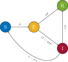
Figure 1: SEIR diagram with transition rates.

When the dynamic is independent from the knowledge of individuals, the model can be expressed by the following system of ODEs

$$\left\{\begin{aligned} \frac{\mathrm{d}S}{\mathrm{d}t}&=-\beta SI+(1-\alpha)\gamma I\\ \frac{\mathrm{d}E}{\mathrm{d}t}&=\beta SI-\delta E\\ \frac{\mathrm{d}I}{\mathrm{d}t}&=(1-\eta)\delta E-\gamma I,\\ \frac{\mathrm{d}R}{\mathrm{d}t}&=\eta\delta E+\alpha\gamma I,\end{aligned}\right.$$ (1)

with $S+E+I+R=1$ and where $\beta$ is the contact rate between the class of the susceptible and the class of infectious, $\delta$ is the rate at which agents make their decision about spreading the news or not, $1-\eta$ is the portion of agents who become infectious and $\gamma$ is the rate at which spreaders remove themselves from the compartment, due, e.g., to loss of interest in sharing the news or forgetfulness. Finally, $\alpha$ is related to the specificity of the fake news and the probability of individulas to remember it. A probability of $0$ means that the fake news has not any inherent peculiarity (e.g., in terms of content, structure, style, …) that can make it memorable enough for the population to ‘immunize’ against it in the future, while a probability of $1$ allows for the agents to have the full ability to not fall for that fake news a second time. The various parameters have been summarized in Table 2. The diagram of the SEIR model (1) is shown in Figure 1.

Parameter	Definition
$\beta$	contact rate between susceptible and infected individuals
$1/\delta$	average decision time on whether or not to spread fake news
$\eta$	probability of deciding not to spread fake news
$1/\gamma$	average duration of a fake news
$\alpha$	probability of remembering fake news

Table 2: Parameters definition in the SEIR model (1).

It is straightforward to notice that when $\alpha$ and $\eta$ are zero, system (1) specializes in a classic SEIS epidemiological model. This is consistent with treating the dissemination of non-specific fake news in a population as the spread of a disease with multiple strains, for which a durable immunization is never attained. In this case system (1) has two equilibrium states: a disease-free equilibrium state $(1,0,0)$ and an endemic equilibrium state $\tilde{P}=(\tilde{S},\tilde{E},\tilde{I})$ where

$$\tilde{S}=\frac{1}{R_{0}},\qquad\tilde{E}=\frac{\gamma}{\gamma+\delta}\biggl{(}1-\frac{1}{R_{0}}\biggr{)},\qquad\tilde{I}=\frac{\delta}{\gamma+\delta}\biggl{(}1-\frac{1}{R_{0}}\biggr{)},$$ (2)

and $R_{0}=\beta/\gamma$ is the basic reproduction number. It is known [21] that if $R_{0}>1$ the endemic equilibrium state $\tilde{P}$ of system (1) is globally asymptotically stable.

If instead $\alpha>0$ or $\eta>0$, there also is the possibility to permanently immunize against fake news with those traits; moreover, both infectious and exposed agents eventually vanish, leaving only the susceptible and removed compartments populated. In the case of maximum specificity of the fake news, i.e., $\alpha=1$, the stationary equilibrium state has the form

$$S(t)\to S^{\infty},\quad E(t)\to 0,\quad I(t)\to 0,\quad R(t)\to R^{\infty}=1-S^{\infty},$$ (3)

where $S^{\infty}$ is solution of the nonlinear equation

$$\log\frac{S_{0}}{S^{\infty}}=\frac{\beta}{\gamma}(1-\eta)(1-S^{\infty}),$$ (4)

in which $S_{0}$ is the initial datum $S(t=0)$.

We refer to [5, 25, 32] for the inclusion of additional interaction dynamics, taking into account counter-information effects due to the removed population interacting against susceptible and infectious, and the relative analysis of the resulting equilibrium states.

2.2 The interplay with competence and learning

In the following, we combine the evolution of the densities according to the SEIR model (1) with the competence dynamics proposed in [29]. We refer to the degree of competence that an individual can gain or loose in a single interaction from the background as $z\in\mathbb{R}^{+}$; in what follows we denote by $C(z)$ the bounded-mean distribution of $z$, satisfying

$$\int_{\mathbb{R}^{+}}C(z)\,\mathrm{d}z=1,\quad\int_{\mathbb{R}^{+}}zC(z)\,\mathrm{d}z=m_{B}.$$

Assuming a susceptible agent has a competence level $x$ and interacts with another one belonging to the various compartments in the population and having a competence level $x_{\ast}$, their levels after the interaction will be given by

$$\left\{\begin{aligned} x^{\prime}&=(1-\lambda_{S}(x))x+\lambda_{CJ}(x)x_{\ast}+\lambda_{BS}(x)z+\kappa_{SJ}x\\ x_{\ast}^{\prime}&=(1-\lambda_{J}(x_{\ast}))x_{\ast}+\lambda_{CS}(x_{\ast})x+\lambda_{BJ}(x_{\ast})z+\tilde{\kappa}_{SJ}x_{\ast},\end{aligned}\right. J\in\{S,E,I,R\}$$ (5)

where $\lambda_{S}(\cdot)$ and $\lambda_{BS}(\cdot)$ quantify the amount of competence lost by susceptible individuals by the natural process of forgetfulness and the amount gained by susceptible individuals from the background, respectively. $\lambda_{CJ}$, instead, models the competence gained through the interaction with members of the class $J$, with $J\in\{S,E,I,R\}$; a possible choice for $\lambda_{CJ}(x)$ is $\lambda_{CJ}(x)=\lambda_{CJ}\chi(x\geq\bar{x})$, where $\chi(\cdot)$ is the characteristic function and $\bar{x}\in X$ a minimum level of competence required to the agents for increasing their own skills by interactions. Finally, $\kappa_{SJ}$ and $\tilde{\kappa}_{SJ}$ are independent and identically distributed zero-mean random variables with the same variance $\sigma(t)$ to consider the non-deterministic nature of the competence acquisition process.

The binary interactions involving the exposed agents can be similarly defined

$$\left\{\begin{aligned} x^{\prime}&=(1-\lambda_{E}(x))x+\lambda_{CJ}(x)x_{\ast}+\lambda_{BE}(x)z+\kappa_{EJ}x\\ x_{\ast}^{\prime}&=(1-\lambda_{J}(x_{\ast}))x_{\ast}+\lambda_{CE}(x_{\ast})x+\lambda_{BJ}(x_{\ast})z+\tilde{\kappa}_{EJ}x_{\ast},\end{aligned}\right. J\in\{S,E,I,R\}$$ (6)

the same holds for the interactions concerning the infectious fraction of the population

$$\left\{\begin{aligned} x^{\prime}&=(1-\lambda_{I}(x))x+\lambda_{CJ}(x)x_{\ast}+\lambda_{BI}(x)z+\kappa_{IJ}x\\ x_{\ast}^{\prime}&=(1-\lambda_{J}(x_{\ast}))x_{\ast}+\lambda_{CI}(x_{\ast})x+\lambda_{BJ}(x_{\ast})z+\tilde{\kappa}_{IJ}x_{\ast},\end{aligned}\right. J\in\{S,E,I,R\}$$ (7)

and finally we have the interactions regarding the removed agents

$$\left\{\begin{aligned} x^{\prime}&=(1-\lambda_{R}(x))x+\lambda_{CJ}(x)x_{\ast}+\lambda_{BR}(x)z+\kappa_{RJ}x\\ x_{\ast}^{\prime}&=(1-\lambda_{J}(x_{\ast}))x_{\ast}+\lambda_{CR}(x_{\ast})x+\lambda_{BJ}(x_{\ast})z+\tilde{\kappa}_{RJ}x_{\ast},\end{aligned}\right. J\in\{S,E,I,R\}.$$ (8)

It is reasonable to assume that both the processes of gain and loss of competence from the interaction with other agents or with the background in (5)–(8) are bounded by zero. Therefore we suppose that if $J,H\in\{S,E,I,R\}$, and if $\lambda_{J}\in[\lambda_{J}^{-},\lambda_{J}^{+}]$, with $\lambda_{J}^{-}>0$ and $\lambda_{J}^{+}<1$, and $\lambda_{CJ}(x),\lambda_{BJ}(x)\in[0,1]$ then $\kappa_{HJ}$ may, for example, be uniformly distributed in $[-1+\lambda_{J}^{+},1-\lambda_{J}^{+}]$.

In order to combine the compartmental model SEIR with the evolution of the competence levels given by equations  (5)–(8) we introduce the interaction operator $Q_{HJ}(\cdot,\cdot)$ following the standard Boltzmann-type theory [27]. As earlier, we will denote with $J$ a suitable compartment of the population, i.e., $H,J\in\{S,E,I,R\}$, and we will use the brackets $\langle\cdot\rangle$ to indicate the expectation with respect to the random variable $\kappa_{HJ}$. Thus, if $\psi(x)$ is an observable function, then the action of $Q_{HJ}(f_{H},f_{J})(x,t)$ on $\psi(x)$ is given by

$$\int_{\mathbb{R}^{+}}Q_{SJ}(f_{S},f_{J})\psi(x)\,\mathrm{d}x=\left\langle\int_{\mathbb{R}^{2}_{+}}f_{S}(x,t)f_{J}(x_{\ast},t)\bigl{(}\psi(x^{\prime})-\psi(x)\bigr{)}\,\mathrm{d}x_{\ast}\mathrm{d}x\right\rangle,$$ (9)

with $x^{\prime}$ defined by (5)

$$\int_{\mathbb{R}^{+}}Q_{EJ}(f_{E},f_{J})\psi(x)\,\mathrm{d}x=\left\langle\int_{\mathbb{R}^{2}_{+}}f_{E}(x,t)f_{J}(x_{\ast},t)\bigl{(}\psi(x^{\prime})-\psi(x)\bigr{)}\,\mathrm{d}x_{\ast}\mathrm{d}x\right\rangle,$$ (10)

with $x^{\prime}$ defined by (6)

$$\int_{\mathbb{R}^{+}}Q_{IJ}(f_{I},f_{J})\psi(x)\,\mathrm{d}x=\left\langle\int_{\mathbb{R}^{2}_{+}}f_{I}(x,t)f_{J}(x_{\ast},t)\bigl{(}\psi(x^{\prime})-\psi(x)\bigr{)}\,\mathrm{d}x_{\ast}\mathrm{d}x\right\rangle,$$ (11)

with $x^{\prime}$ defined by (7),

$$\int_{\mathbb{R}^{+}}Q_{RJ}(f_{R},f_{J})\psi(x)\,\mathrm{d}x=\left\langle\int_{\mathbb{R}^{2}_{+}}f_{R}(x,t)f_{J}(x_{\ast},t)\bigl{(}\psi(x^{\prime})-\psi(x)\bigr{)}\,\mathrm{d}x_{\ast}\mathrm{d}x\right\rangle,$$ (12)

with $x^{\prime}$ defined by (8). All the above operators preserve the total number of agents as the unique interaction invariant, corresponding to $\psi(\cdot)\equiv 1$.

The system then reads:

$$\left\{\begin{aligned} \frac{\partial f_{S}(x,t)}{\partial t}&=-K(x,t)f_{S}(x,t)+(1-\alpha(x))\gamma(x)f_{I}(x,t)+\sum_{\mathclap{J\in\{S,E,I,R\}}}Q_{SJ}(f_{S},f_{J})(x,t),\\ \frac{\partial f_{E}(x,t)}{\partial t}&=K(x,t)f_{S}(x,t)-\delta(x)f_{E}(x,t)+\sum_{\mathclap{J\in\{S,E,I,R\}}}Q_{EJ}(f_{E},f_{J})(x,t),\\ \frac{\partial f_{I}(x,t)}{\partial t}&=\delta(x)(1-\eta(x))f_{E}(x,t)-\gamma(x)f_{I}(x,t)+\sum_{\mathclap{J\in\{S,E,I,R\}}}Q_{IJ}(f_{I},f_{J})(x,t),\\ \frac{\partial f_{R}(x,t)}{\partial t}&=\delta(x)\eta(x)f_{E}(x,t)+\alpha(x)\gamma(x)f_{I}(x,t)+\sum_{\mathclap{J\in\{S,E,I,R\}}}Q_{RJ}(f_{R},f_{J})(x,t),\end{aligned}\right.$$ (13)

where the function

$$K(x,t)=\int_{\mathbb{R}^{+}}\beta(x,x_{\ast})f_{I}(x_{\ast},t)\,\mathrm{d}x_{\ast}$$

is responsible for the contagion, $\beta(x,x_{\ast})$ being the contact rate between agents with competence levels $x$ and $x_{\ast}$. In the above formulation we also assumed $\beta$, $\gamma$, $\delta$, $\eta$ and $\alpha$ functions of $x$. Note that, clearly, the most important parameters influenced by individuals’ competence are $\beta(x,x_{\ast})$, since individuals have the highest rates of contact with people belonging to the same social class, and thus with a similar level of competence, $\delta(x)$ as individuals with greater competence invest more time in checking the authenticity of information, and $\eta(x)$, which characterizes individuals’ decision to spread fake news. On the other hand, the values of $\gamma$ and $\alpha$ we may assume to be less influenced by the level of expertise of individuals.

2.3 Properties of the kinetic SEIR model with competence

In this section we analyze some of the properties of the Boltzmann system (13). First let us consider the reproducing ratio in presence of knowledge.

By integrating system (13) against $x$, and considering only the compartments of individuals which may disseminate the fake news we have

$$\left\{\begin{aligned} \frac{\mathrm{d}E(t)}{\mathrm{d}t}&=\int_{X}K(x,t)f_{S}(x,t)\,dx-\int_{X}\delta(x)f_{E}(x,t)\,dx,\\ \frac{\mathrm{d}I(t)}{\mathrm{d}t}&=\int_{X}\delta(x)(1-\eta(x))f_{E}(x,t)\,dx-\int_{X}\gamma(x)f_{I}(x,t)\,dx.\\ \end{aligned}\right.$$ (14)

In the above derivation we used the fact that the Boltzmann interaction terms describing knowledge evolution among agents preserve the total number of individuals and therefore vanish. Following the analysis in [4], and omitting the details for brevity, we obtain a reproduction number generalizing the classical one

$$R_{0}(t)=\frac{\int_{X}K(x,t)f_{S}(x,t)\,dx}{\int_{X}\gamma(x)f_{I}(x,t)\,dx}.$$ (15)

Next, following [15], we can prove uniqueness of the solution of (13) in the simplified case of constant parameters: $\beta(x,x_{\ast})=\beta>0$, $\gamma(x)=\gamma>0$, $\delta(x)=\delta>0$, $\eta(x)=\eta\in[0,1]$, $\alpha(x)=\alpha\in[0,1]$. In this case, exploiting the fact that the interaction operator $Q(\cdot,\cdot)$ has a natural connection with the Fourier transform by choosing its kernel $\mathrm{e}^{-ix\xi}$ as test function, we can analyze the system (13) with the Fourier transforms of the densities as unknowns.

Indeed, given a function $f(x)\in L_{1}(\mathbb{R}^{+})$, its Fourier transform is defined as

$$\hat{f}(\xi)=\int_{\mathbb{R}}\mathrm{e}^{-ix\xi}f(x)\,\mathrm{d}x.$$

The system (13) becomes

$$\left\{\begin{aligned} \frac{\partial\hat{f}_{S}(\xi,t)}{\partial t}&=-\beta I(t)\hat{f}_{S}(\xi,t)+(1-\alpha)\gamma\hat{f}_{I}(\xi,t)+\sum_{\mathclap{J\in\{S,E,I,R\}}}\hat{Q}_{SJ}(\hat{f}_{S},\hat{f}_{J})(\xi,t),\\ \frac{\partial\hat{f}_{E}(\xi,t)}{\partial t}&=\beta I(t)\hat{f}_{S}(\xi,t)-\delta\hat{f}_{E}(\xi,t)+\sum_{\mathclap{J\in\{S,E,I,R\}}}\hat{Q}_{EJ}(\hat{f}_{E},\hat{f}_{J})(\xi,t),\\ \frac{\partial\hat{f}_{I}(\xi,t)}{\partial t}&=\delta(1-\eta)\hat{f}_{E}(\xi,t)-\gamma\hat{f}_{I}(\xi,t)+\sum_{\mathclap{J\in\{S,E,I,R\}}}\hat{Q}_{IJ}(\hat{f}_{I},\hat{f}_{J})(\xi,t),\\ \frac{\partial\hat{f}_{R}(\xi,t)}{\partial t}&=\delta\eta\hat{f}_{E}(\xi,t)+\alpha\gamma\hat{f}_{I}(\xi,t)+\sum_{\mathclap{J\in\{S,E,I,R\}}}\hat{Q}_{RJ}(\hat{f}_{R},\hat{f}_{J})(\xi,t),\end{aligned}\right.$$ (16)

where the operators $\hat{Q}_{HJ}(\hat{f}_{H},\hat{f}_{J})$ are defined in terms of the Fourier transforms of their arguments for $J\in\{S,E,I,R\}$, so that

$$\hat{Q}_{HJ}(\hat{f}_{H},\hat{f}_{J})=\langle\hat{f}_{H}(A_{HJ}\xi-\lambda_{BH}z,t)\rangle\hat{f}_{J}(\lambda_{CJ}\xi,t)-\hat{f}_{H}(\xi,t)J(t),$$

where $A_{HJ}$, with $H,J\in\{S,E,I,R\}$ is defined as

$$A_{HJ}=1-\lambda_{H}+\kappa_{H}.$$ (17)

We suppose that the parameters satisfy the condition

$$\nu=\max_{H,J\in\{S,E,I,R\}}[\lambda_{CJ}^{2}+\langle A_{JH}^{2}\rangle]<1,$$ (18)

which will prove useful in the proof.

As in [15] we recall a class of metrics which is of natural use in bilinear Boltzmann equations [27]. Let $f$ and $g$ be probability densities. Then, for $s>0$ we define

$$d_{s}(f,g)=\sup_{\xi\in\mathbb{R}}\frac{\lvert\hat{f}(\xi)-\hat{g}(\xi)\rvert}{\lvert\xi\rvert^{s}},$$ (19)

which is finite whenever $f$ and $g$ have equal moments up to the integer part of $s$ or to $s-1$ if $s$ is an integer.

We have the following result.

Theorem 1.

Let $J\in\{S,E,I,R\}$, and let $f_{J}(x,t)$ and $g_{J}(x,t)$ be two solutions of the system (13) with initial values $f_{J}(x,0)$ and $g_{J}(x,0)$ such that $d_{2}(f_{J}(x,0),g_{J}(x,0)$ is finite. Then, condition (18) implies that the Fourier based distance $d_{2}(f_{J}(x,t),g_{J}(x,t)$ decays exponentially (in time) to zero, so that

$$\sum_{\mathclap{J\in\{S,E,I,R\}}}d_{2}(f_{J}(x,t),g_{J}(x,t)\leq\sum_{\mathclap{J\in\{S,E,I,R\}}}d_{2}(f_{J}(x,0),g_{J}(x,0)\mathrm{e}^{-(1-\nu)t}.$$

For the details of the proof we refer to Appendix A.

3 Mean-field approximation

A highly useful tool to obtain information analytically on the large-time behavior of Boltzmann-type models are scaling techniques; in particular the so-called quasi-invariant limit [27], which allows to derive the corresponding mean-field description of the kinetic model (13).

Indeed, let us consider the case in which the interactions between agents produce small variations of the competence. We scale the quantities involved in the binary interactions (5)-(8) accordingly

$$\lambda_{CJ}\to\varepsilon\lambda_{CJ}, \lambda_{BJ}\to\varepsilon\lambda_{BJ}, \lambda_{J}\to\varepsilon\lambda_{J}, \sigma\to\varepsilon\sigma,$$ (20)

where $J\in\{S,E,I,R\}$ and the functions involved in the dissemination of the fake news, as well

$$\beta(x,x_{\ast})\to\varepsilon\beta(x,x_{\ast}), \gamma(x)\to\varepsilon\gamma(x), \delta(x)\to\varepsilon\delta(x), \eta(x)\to\varepsilon\eta(x).$$ (21)

We denote by $Q^{\varepsilon}_{HJ}(\cdot,\cdot)$ the scaled interaction terms. Omitting the dependence on time on mean values and re-scaling time as $t\to t/\varepsilon$, we obtain up to $\mathcal{O}(\varepsilon)$

$$\frac{1}{\varepsilon}\int_{\mathbb{R}^{+}}Q_{SJ}^{\varepsilon}(f_{S},f_{J})\psi(x)\,\mathrm{d}x \approx\int_{\mathbb{R}^{+}}\biggl{[}-\psi(x)^{\prime}(\lambda_{S}xJ-\lambda_{CJ}m_{J}-\lambda_{BS}m_{B}J)+\frac{\sigma}{2}\psi(x)^{\prime\prime}x^{2}J\biggr{]}f_{S}(x,t)\,\mathrm{d}x$$

$$\frac{1}{\varepsilon}\int_{\mathbb{R}^{+}}Q_{EJ}^{\varepsilon}(f_{E},f_{J})\psi(x)\,\mathrm{d}x \approx\int_{\mathbb{R}^{+}}\biggl{[}-\psi(x)^{\prime}(\lambda_{E}xJ-\lambda_{CJ}m_{J}-\lambda_{BE}m_{B}J)+\frac{\sigma}{2}\psi(x)^{\prime\prime}x^{2}J\biggr{]}f_{E}(x,t)\,\mathrm{d}x$$

$$\frac{1}{\varepsilon}\int_{\mathbb{R}^{+}}Q_{IJ}^{\varepsilon}(f_{I},f_{J})\psi(x)\,\mathrm{d}x \approx\int_{\mathbb{R}^{+}}\biggl{[}-\psi(x)^{\prime}(\lambda_{I}xJ-\lambda_{CJ}m_{J}-\lambda_{BI}m_{B}J)+\frac{\sigma}{2}\psi(x)^{\prime\prime}x^{2}J\biggr{]}f_{I}(x,t)\,\mathrm{d}x$$

$$\frac{1}{\varepsilon}\int_{\mathbb{R}^{+}}Q_{RJ}^{\varepsilon}(f_{R},f_{J})\psi(x)\,\mathrm{d}x \approx\int_{\mathbb{R}^{+}}\biggl{[}-\psi(x)^{\prime}(\lambda_{R}xJ-\lambda_{CJ}m_{J}-\lambda_{BR}m_{B}J)+\frac{\sigma}{2}\psi(x)^{\prime\prime}x^{2}J\biggr{]}f_{R}(x,t)\,\mathrm{d}x,$$

where we used a Taylor expansion for small values of $\varepsilon$ of

$$\psi(x^{\prime})=\psi(x)+(x^{\prime}-x)\psi^{\prime}(x)+\frac{(x^{\prime}-x)^{2}}{2}\psi^{\prime\prime}(x)+\mathcal{O}(\varepsilon^{2})$$

in (9)-(12) and the scaled interaction rules (5)-(8).

3.1 Stationary solutions of Fokker-Planck SEIR models

Let us impose that $\varepsilon\to 0$, following [27] from the computations of the previous section we formally obtain the Fokker-Planck system

$$\frac{\partial f_{S}(x,t)}{\partial t} =-K(x,t)f_{S}(x,t)+(1-\alpha(x))\gamma(x)f_{I}(x,t)+\frac{\partial}{\partial x}[(x\lambda_{S}-\overline{m}(t)-\lambda_{BS}m_{B})f_{S}(x,t)]$$

$$\phantom{=}{}+\frac{\sigma}{2}\frac{\partial^{2}}{\partial x^{2}}(x^{2}f_{S}(x,t))$$ (22)

$$\frac{\partial f_{E}(x,t)}{\partial t} =K(x,t)f_{S}(x,t)-\delta(x)f_{E}(x,t)+\frac{\partial}{\partial x}[(x\lambda_{E}-\overline{m}(t)-\lambda_{BE}m_{B})f_{E}(x,t)]$$

$$\phantom{=}{}+\frac{\sigma}{2}\frac{\partial^{2}}{\partial x^{2}}(x^{2}f_{E}(x,t))$$ (23)

$$\frac{\partial f_{I}(x,t)}{\partial t} =\delta(x)(1-\eta(x))f_{E}(x,t)-\gamma(x)f_{I}(x,t)+\frac{\partial}{\partial x}[(x\lambda_{I}-\overline{m}(t)-\lambda_{BI}m_{B})f_{I}(x,t)]$$

$$\phantom{=}{}+\frac{\sigma}{2}\frac{\partial^{2}}{\partial x^{2}}(x^{2}f_{I}(x,t))$$ (24)

$$\frac{\partial f_{R}(x,t)}{\partial t} =\delta(x)\eta(x)f_{E}(x,t)+\alpha(x)\gamma(x)f_{I}(x,t)+\frac{\partial}{\partial x}[(x\lambda_{R}-\overline{m}(t)-\lambda_{BR}m_{B})f_{R}(x,t)]$$

$$\phantom{=}{}+\frac{\sigma}{2}\frac{\partial^{2}}{\partial x^{2}}(x^{2}f_{R}(x,t))$$ (25)

where now

$$\overline{m}(t)=\lambda_{CS}m_{S}(t)+\lambda_{CE}m_{E}(t)+\lambda_{CI}m_{I}(t)+\lambda_{CR}m_{R}(t).$$

We can consider the mean values system associated to (22)–(25) in the case of constant epidemiological parameters

$$\frac{\mathrm{d}m_{S}(t)}{\mathrm{d}t} =-\beta I(t)m_{S}(t)+(1-\alpha)\gamma m_{I}(t)+\lambda S(t)(m(t)-m_{B})/2-\lambda m_{S}(t)$$ (26)

$$\frac{\mathrm{d}m_{E}(t)}{\mathrm{d}t} =\beta I(t)m_{S}(t)-\delta m_{E}(t)+\lambda E(t)(m(t)-m_{B})/2-\lambda m_{E}(t)$$ (27)

$$\frac{\mathrm{d}m_{I}(t)}{\mathrm{d}t} =\delta(1-\eta)m_{E}(t)-\gamma m_{I}(t)+\lambda I(t)(m(t)-m_{B})/2-\lambda m_{I}(t)$$ (28)

$$\frac{\mathrm{d}m_{R}(t)}{\mathrm{d}t} =\delta\eta m_{E}(t)+\alpha\gamma m_{I}(t)+\lambda R(t)(m(t)-m_{B})/2-\lambda m_{R}(t),$$ (29)

with

$$m(t)=m_{S}(t)+m_{E}(t)+m_{I}(t)+m_{R}(t).$$

In the case $\alpha>0$ or $\eta>0$, we know that $E(t)\to 0$, $I(t)\to 0$, $S(t)\to S^{\infty}$ and $R(t)\to R^{\infty}=1-S^{\infty}$ due to mass conservation, so that $m_{E}(t)\to 0$ and $m_{I}(t)\to 0$ as well. Thus, adding all the equations together leads us to

$$\frac{\lambda}{2}(m_{S}^{\infty}+m_{R}^{\infty})+\frac{\lambda}{2}m_{B} =\lambda(m_{S}^{\infty}+m_{R}^{\infty}),$$ (30)

i.e., $m_{S}^{\infty}+m_{R}^{\infty}=m_{B}$. At this point, adding together equations (22) to (25) gives us

$$0=\lambda\frac{\partial}{\partial x}(x-m_{B})\sum_{\mathclap{J\in\{S,R\}}}f_{J}^{\infty}(x)+\frac{\sigma}{2}\frac{\partial^{2}}{\partial x^{2}}\biggl{(}x^{2}\sum_{\mathclap{\quad J\in\{S,R\}}}f_{J}^{\infty}(x)\biggr{)},$$

which has as solution an inverse Gamma density

$$f^{\infty}(x)=f_{S}^{\infty}(x)+f_{R}^{\infty}(x)=\frac{k^{\mu}}{\Gamma(\mu)}\frac{\mathrm{e}^{-k/x}}{x^{1+\mu}},$$ (31)

$$\mu=1+\frac{2\lambda}{\sigma}, \quad k=(\mu-1)m_{B}.$$

It is straightforward to see that the scaled Gamma densities

$$f_{S}^{\infty}(x)=S^{\infty}\frac{k^{\mu}}{\Gamma(\mu)}\frac{\mathrm{e}^{-k/x}}{x^{1+\mu}}\quad f_{R}^{\infty}(x)=(1-S^{\infty})\frac{k^{\mu}}{\Gamma(\mu)}\frac{\mathrm{e}^{-k/x}}{x^{1+\mu}}$$

are solutions of the system (22)–(25).

If, instead, $\alpha=\eta=0$, we find again the same solution as (31), but in this case $J\to\tilde{J}$, where $\tilde{J}$ are defined as in (2).

In Figure 2 we report two examples of the stationary solutions where we chose the competence variable $z$ to be uniformly distributed in $[0,1]$: in the first case (left) we considered $\alpha=\eta=0$, while in the second case (right) we set $\alpha=0.2$ and $\eta=0.1$.

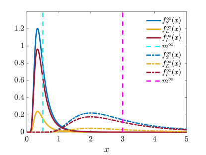
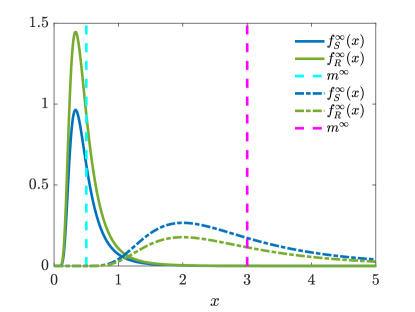
Figure 2: Exact solutions for competence distributions at the end of epidemic(31) for $\lambda=0.1$, $\mu=5$, $m_{B}=0.5$ (solid), $m_{B}=3$ (dash-dotted), $\tilde{S}=0.5$, $\tilde{E}=0.1$, $\tilde{I}=0.4$ (left) and $S^{\infty}=0.6$, $R^{\infty}=0.4$ (right). Left: case $\alpha=\eta=0$; right: case $\alpha=0.2$, $\eta=0.1$.

4 Numerical examples

In this section we present some numerical tests to show the characteristics of the model in describing the dynamics of fake news dissemination in a population with a competence-based structure.

To begin with, we validate the Fokker-Planck model obtained as the quasi-invariant limit of the Boltzmann equation: we will do so through a Monte Carlo method for the competence distribution (see [27], Chapter 5 for more details). Next, we approximate the Fokker-Planck systems (22)–(25) by generalizing the structure-preserving numerical scheme [30] to explore the interplay between competence and disseminating dynamics in the more realistic case of epidemiological parameters dependent on the competence level (see Appendix B). Lastly, we investigate how the fake news’ diffusion would impact differently on different classes of the population defined in terms of their capabilities of interacting with information.

4.1 Test 1: Numerical quasi-invariant limit

In this test we show that the mean-field Fokker-Planck system (22)–(25) obtained under the quasi-invariant scaling (20) and (21) is a good approximation of the Boltzmann models (13) when $\varepsilon\ll 1$. We do so by using a Monte Carlo method with $N=10^{4}$ particles, starting with a uniform distribution of competence $f_{0}(x)=\frac{1}{2}\chi(x\in[0,2])$, where $\chi(\cdot)$ is the indicator function, and performing various iterations until the stationary state was reached; next, the distributions were averaged over the next 500 iterations. We considered constant competence-related parameters $\lambda_{CJ}=\lambda_{BJ}$ and $\lambda_{J}=\lambda_{CJ}+\lambda_{BJ}$ as well as a constant variance $\sigma$ for the random variables $\eta_{HJ}$.

In Figure 3, we plotted the results for $(\lambda,\sigma)=(0.075,0.150)$ (circle-solid, teal) and for $(\lambda,\sigma)=(0.001,0.002)$ (square-solid, ochre): those choices correspond to a scaling regime of $\varepsilon=0.075$ and $\varepsilon=0.001$, respectively, with $\mu=2$. Finally, we assumed that $m_{B}=0.75$ (left) and $m_{B}=1$ (right).

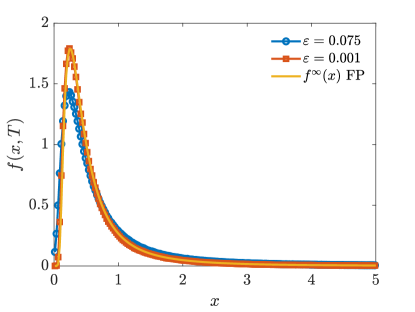
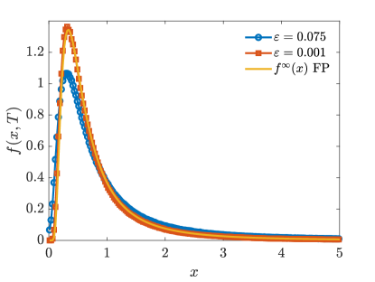
Figure 3: Test 1. Comparison of the competence distributions at the end of epidemics for system (13) with the explicit Fokker-Planck solution (31) with scaling parameters $\varepsilon=0.075,0.001$. We considered the case $m_{B}=0.75$ (left) and $m_{B}=1$ (right).

Directly comparing the Boltzmann dynamics equilibrium with the explicit analytic solution of the Fokker-Planck regime shows that if $\varepsilon$ is small enough, Fokker-Planck asymptotics provide a consistent approximation of the steady states of the kinetic distributions.

4.2 Test 2: Learning dynamics and fake news dissemination

For this test, we applied the structure-preserving scheme to system (22)–(25) in a more realistic scenario featuring an interaction term dependent on the competence level of the agents, as well as a competence-dependent delay during which agents evaluate the information and decide how to act. In this setting, we refer to the recent Survey of Adult Skills (SAS) made by the OECD [26]: in particular, we focus on competence understood as a set of information-processing skills, especially through the lens of literacy, defined [26] as “the ability to understand, evaluate, use and engage with written texts in order to participate in society”. One of the peculiarities that makes the SAS, which is an international, multiple-year spanning effort in the framework of the PIAAC (Programme for the International Assessment of Adult Competencies) by the OECD, interesting in our case is that it was administered digitally to more than 70% of the respondents. Digital devices are arguably the most important vehicle for information diffusion in OECD countries, so that helps to keep consistency.

Literacy proficiency was defined through $6$ increasing levels; we therefore consider a population partitioned in $6$ classes based on the competence level of their occupants, equated to the score of the literacy proficiency test of the SAS, normalized. Thus, we chose a log-normal-like distribution

$$f(x)=\frac{1}{(\tilde{\xi}-x)\tilde{\sigma}\sqrt{2\pi}}\cdot\mathrm{e}^{-\frac{(\log(\tilde{\xi}-x)-\tilde{\mu})^{2}}{2\tilde{\sigma}^{2}}},$$

where $\tilde{\xi}=5$, $\tilde{\mu}\approx 0.85$ and $\tilde{\sigma}\approx 0.22$ to make $f(x)$ agree with the empirical findings in [26]. The computational domain is restricted to $x\in[0,5]$ and stationary boundary conditions have been applied as described in Appendix B.

Initial distributions for the epidemiological compartments were set as

$$f_{S}(x,0)=\rho_{S}f(x),\quad f_{E}(x,0)=\rho_{E}f(x),\quad f_{I}(x,0)=\rho_{I}f(x),\quad f_{R}(x,0)=\rho_{R}f(x),$$

with $\rho_{I}=10^{-2}$, $\rho_{S}=1-\rho_{I}$ and $\rho_{E}=\rho_{R}=0$.

The contact rate $\beta(x,x_{*})$ was set as

$$\beta(x,x_{*})=\frac{\beta_{0}}{(1+x^{2})(1+x_{*}^{2})}\chi(\lvert x-x_{*}\rvert\leq\Delta)$$ (32)

with $\Delta=2$ on the hypothesis that interactions occur more frequently among people with a similar competence level and are higher for people with lower competence levels.

The rate $\delta$ at which the information is evaluated by the agents, who therefore exits the exposed class, was set to be

$$\delta(x)=\delta_{R}+(\delta_{L}-\delta_{R})\frac{1}{1+\mathrm{e}^{a(b-x)}},$$ (33)

with $\delta_{L}=1$, $\delta_{R}=5$, $a=2$ and $b=2.5$. Here, we are taking into account that people with higher efficacy at identifying fake news spend significantly more time on conducting their evaluations than people with lower efficacy [23]. In this specific test case the time range for the evaluation of the information spans between 1 day and about 5 hours. The values were purposely chosen rather large compared to realistic values in order to highlight also the behavior of the exposed compartment. Finally, we set $\gamma=0.2$, which correspond to an average fake news duration of 5 days, and $\alpha=0.2$, so that individuals have a moderate possibility to remember the fake news and become immune to it, and assume $\eta=0.1$, namely in this test we do not relate the decision to spread or not fake news to the level of competence.

We investigate the relation between the dissemination-related component of the model and the competence-related one, which entails that agents can learn, i.e., increase their competence level, both from the background and from direct binary interactions. Under the assumption that $\lambda_{CJ}+\lambda_{BJ}=\lambda_{J}$, which is a conservative choice: the expected value of the competence gained through interactions cancels out the one lost due to forgetfulness, in this latter process two main parameters are involved: $\lambda=\lambda_{J}$ (i.e., all compartments have the same learning rate) and $m_{B}$, which is the mean of the background competence variable $z$.

For what concerns the dissemination-related component, instead, the main factor is the reproduction number $R_{0}$ (15). Hence, we measured the differences on the spread of fake news varying these three parameters. In Figure 4 (left) we show the highest portion of spreaders in relation to the mean of background $m_{B}$ and to the reproduction number $R_{0}$; in the right image $\lambda$ is opposed to $R_{0}$.

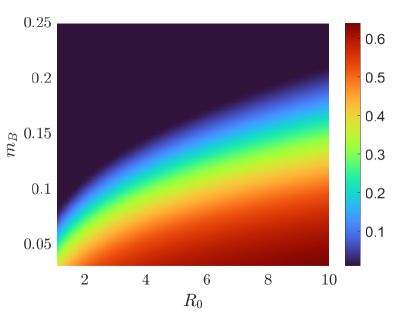
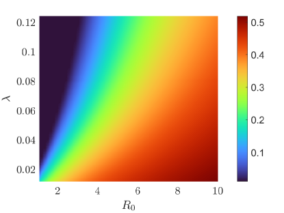
Figure 4: Test 2. Interplay between competence levels and dissemination dynamics. Contour plots of the highest number of infected in relation to the reproduction number (15) $R_{0}\in[1.1,10]$ and the background competence mean $m_{B}\in[0.03125,0.25]$ (left) and learning rate $\lambda\in[0.0125,0.125]$ (right).

To perform the test, we leveraged the structure-preserving numerical scheme [30] whose details are presented for convenience in Appendix B. In both images of Figure 4 we see transition effects: the learning process triggered by the competence dynamics is capable of slowing down the dissemination of fake news in the population, even to the point of preventing it to take place. In the first case, the mean of the background $m_{B}$, i.e., the mean of the distribution of the background competence variable $z$, which we assumed uniformly distributed, varies between $0.03125$ and $0.25$, while the reproduction number $R_{0}$ varies between $1.1$ and $10$. In the second case, we left untouched $R_{0}$, while $\lambda$ varies between $0.0125$ and $0.125$ with a background mean $m_{B}=0.125$. We can see that the mean of the background has a more pronounced impact on the slowing of the diffusion of fake news, with a steeper transition effect.

4.3 Test 3: Impact of the different competence levels

In this final test we considered how much of an impact the competence level can have on the dissemination of fake news in the population. We simulated the mean-field model (22)–(25) assuming the same competence-dependent contact rate $\beta(x,x_{*})$ of Test 2, in this case with $\beta_{0}=4$, as well the same delay rate $\delta(x)$ and the same $\gamma$, but we additionally assume that the decision to spread or not a fake news is affected by the level of competence. This is somewhat controversial in the literature since other factors also affect this behavior like the age of individuals (tests carried out on young people have shown independence from the competence in the decision to share a fake news in contrast to what happens in in older people, see [26, 23]). To emphasize this effect we assume

$$\eta(x)=1-e^{-kx^{2}},$$ (34)

with $k=0.1$. Thus individuals with high level of competence rarely decide to spread fake news.

In Figure 5 we report the time evolution of the distributions of susceptible (top left), exposed (top right), infected (bottom left) and removed (bottom right) agents with competence parameters of $\lambda_{BJ}=\lambda_{CJ}=0.125$, $\lambda_{J}=\lambda_{BJ}+\lambda_{CJ}$ and $m_{B}=0.125$, in the case $\alpha=0.1$. In Figure 6, instead, we show the evolution with the same parameters except for a larger probability $\alpha=0.9$ of remembering the fake news.

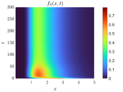
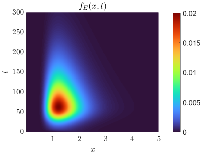
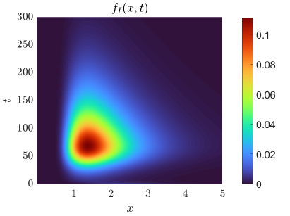
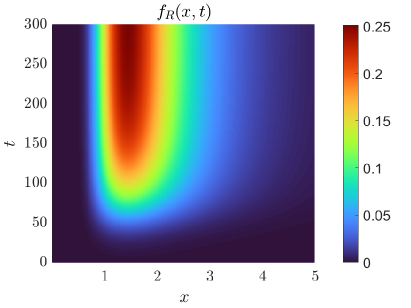
Figure 5: Test 3. Time evolution of the competence distribution for the kinetic model (13) with competence parameters $\lambda_{BJ}=\lambda_{CJ}=0.125$, $\lambda_{J}=\lambda_{BJ}+\lambda_{CJ}$, with a background competence mean of $m_{B}$ = 0.125. We considered $\alpha=0.1$, $\beta_{0}=4$, $\gamma=0.2$. Top left: susceptible; top right: exposed; bottom left: infected; bottom right: removed.

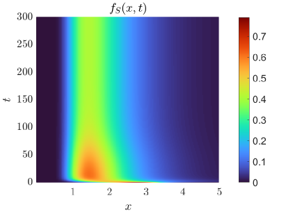
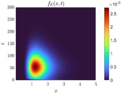
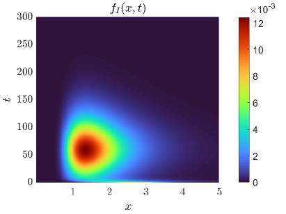
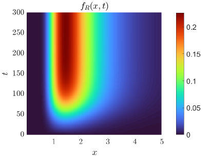
Figure 6: Test 3. Time evolution of the competence distribution for the kinetic model (13) with competence parameters $\lambda_{BJ}=\lambda_{CJ}=0.125$, $\lambda_{J}=\lambda_{BJ}+\lambda_{CJ}$, with a background competence mean of $m_{B}$ = 0.125. We considered $\alpha=0.9$, $\beta_{0}=4$, $\gamma=0.2$. Top left: susceptible; top right: exposed; bottom left: infected; bottom right: removed.

In Figure 7 are shown the relative numbers of susceptible, exposed, infected and removed agents, on the left for $\alpha=0.1$ and on the right for $\alpha=0.9$.

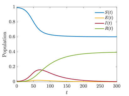
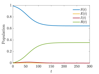
Figure 7: Test 3. Evolution in time of the densities for susceptible, exposed, infectious and removed agents. Left: $\alpha=0.1$; right: $\alpha=0.9$.

To measure the effects of the competence, we considered the curve of the infected agents depending on their levels accordingly to [26] for $x\in[0,5]$:

• below level 1: scoring less then 175/500, ($x<1.75$);

• level 1: scoring between 176/500 and 225/500, ($x>1.75$ and $x<2.25$);

• level 2: scoring between 226/500 and 275/500, ($x>2.25$ and $x<2.75$);

• level 3: scoring between 276/500 and 325/500, ($x>2.75$ and $x<3.25$);

• level 4: scoring between 326/500 and 375/500, ($x>3.25$ and $x<3.75$);

• level 5: scoring more than 375/500, ($x>3.75$).

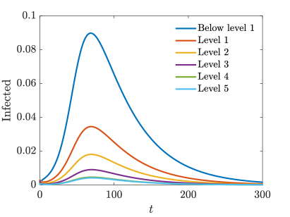
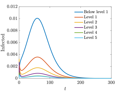
Figure 8: Test 3. Evolution of the fraction of infectious agents with different levels of competence as defined in [26]. Left: $\alpha=0.1$; right: $\alpha=0.9$.

Figure 8 shows clearly that the more competent the individual, the lesser they contribute to the spread of fake news, in perfect agreement with the transition effects observed in Test 4.2 due to the interplay between competence and the dissemination dynamics. Moreover, we can see how the probability $\alpha$ of detecting fake news influences its dissemination in the population: a lower probability implies a higher peak of infected agents for each competence level, as well as a slower spread overall.

5 Concluding remarks

In this paper, we introduced a compartmental model for fake news dissemination that also considers the competence of individuals. In the model, the concept of competence is not introduced as a static feature of the dynamic, but as an evolutionary component that takes into account both learning through interactions between agents and interventions aimed at educating individuals in the ability to detect fake news.

From a mathematical viewpoint the competence dynamics has been introduced as a Boltzmann interaction term in the corresponding system of differential equations. A suitable scaling limit, permits to recover the corresponding Fokker-Planck models and then the resulting stationary states in terms of competence. These, in agreement with [29], are given explicitly by Gamma distributions.

The numerical results demonstrate the model’s ability to correctly describe the interplay between fake news dissemination and individuals’ level of competence, highlighting transition phenomena at the level of expertise that allow fake news to spread more rapidly.

Future developments of the model will be considered in particular in the case of networks, in order to describe the spread of fake news on social networks and present plausible scenarios useful to limit the spread of false information. This can be done by following an approach similar to that of kinetic models for opinion formation on networks [1]. Another challenging aspect concerns the matching of the model with realistic data that requires the introduction of quantitative aspects not always easy to identify [25, 36]. One of the main applications will be related to combating misinformation in the vaccination campaign against COVID-19.

Appendix A Proof of Theorem 1

We provide here a proof for Theorem 1. The proof is identical to [15]; we develop it here, too, for completeness, only in the case $\alpha=\eta=0$. If $H\in\{S,E,I\}$ we have

$$\sum_{\mathclap{J\in\{S,E,I\}}}\hat{Q}(\hat{f}_{H},\hat{f}_{J})(\xi,t) =\sum_{\mathclap{J\in\{S,E,I\}}}\langle\hat{f}_{H}(A_{HJ}\xi-\lambda_{BH}z,t)\rangle\hat{f}_{J}(\lambda_{CJ}\xi,t)-\sum_{\mathclap{J\in\{S,E,I\}}}\hat{f}_{H}(\xi,t)J(t)$$ (35)

$$=\hat{Q}_{+}(\hat{f}_{H})(\xi,t)-\hat{H}(\xi,t)$$

where the second equality follows from mass conservation. In (35), we have defined $\hat{Q}_{+}(\hat{f}_{H})(\xi,t)$ as

$$\hat{Q}_{+}(\hat{f}_{H})(\xi,t)=\sum_{\mathclap{J\in\{S,E,I\}}}\langle\hat{f}_{H}(A_{HJ}\xi-\lambda_{BH}z,t)\rangle\hat{f}_{J}(\lambda_{CJ}\xi,t),$$

where $A_{HJ}$ has been defined originally in (17). Thus, now system (16) reads

$$\left\{\begin{aligned} \frac{\partial\hat{f}_{S}(\xi,t)}{\partial t}+\hat{f}_{S}(\xi,t)&=-\beta I(t)\hat{f}_{S}(\xi,t)+\gamma\hat{f}_{I}(\xi,t)+\hat{Q}_{+}(\hat{f}_{I})(\xi,t)\\ \frac{\partial\hat{f}_{E}(\xi,t)}{\partial t}+\hat{f}_{E}(\xi,t)&=\beta I(t)\hat{f}_{S}(\xi,t)-\delta\hat{f}_{E}(\xi,t)+\hat{Q}_{+}(\hat{f}_{E})(\xi,t)\\ \frac{\partial\hat{f}_{I}(\xi,t)}{\partial t}+\hat{f}_{I}(\xi,t)&=\delta\hat{f}_{E}(\xi,t)-\gamma\hat{f}_{I}(\xi,t)+\hat{Q}(\hat{f}_{I})(\xi,t),\end{aligned}\right.$$ (36)

To ensure positivity of all coefficients on the right-hand side (since $I(t)<1$ and $\beta,\gamma,\delta<1$ we can add $\hat{f}_{J}(\xi,t)$ to each side, where $J$ equals $S$, $E$ and $I$ in the first, second and third equation, respectively, to resort to the equivalent system

$$\left\{\begin{aligned} \frac{\partial\hat{f}_{S}(\xi,t)}{\partial t}+2\hat{f}_{S}(\xi,t)&=(1-\beta I(t))\hat{f}_{S}(\xi,t)+\gamma\hat{f}_{I}(\xi,t)+\hat{Q}_{+}(\hat{f}_{I})(\xi,t)\\ \frac{\partial\hat{f}_{E}(\xi,t)}{\partial t}+2\hat{f}_{E}(\xi,t)&=\beta I(t)\hat{f}_{S}(\xi,t)(1-\delta)\hat{f}_{E}(\xi,t)+\hat{Q}_{+}(\hat{f}_{E})(\xi,t)\\ \frac{\partial\hat{f}_{I}(\xi,t)}{\partial t}+2\hat{f}_{I}(\xi,t)&=\delta\hat{f}_{E}(\xi,t)(1-\gamma)\hat{f}_{I}(\xi,t)+\hat{Q}(\hat{f}_{I})(\xi,t),\end{aligned}\right.$$ (37)

in which all coefficients on the right-hand side are positive.

Now, let $\hat{f}_{J}(\xi,t)$ and $\hat{g}(\xi,t)$ be two solutions of the system (37). We look at the time behavior of the $d_{2}$ metric of their difference, where the Fourier-based metric was defined in (19); therefore we define

$$h_{J}(\xi,t)=\frac{\hat{f}_{J}(\xi,t)-\hat{g}_{J}(\xi,t)}{\lvert\xi\rvert^{2}}.$$

We see that the metric and $h_{J}$ are related by

$$d_{2}(f_{J},g_{J})=\lVert h_{J}\rVert_{\infty}$$ (38)

By its definition, the $h_{J}$ are solutions of

$$\left\{\begin{aligned} \frac{\partial\hat{h}_{S}(\xi,t)}{\partial t}+2\hat{h}_{S}(\xi,t)&=(1-\beta I(t))\hat{h}_{S}(\xi,t)+\gamma\hat{h}_{I}(\xi,t)+L_{+}(\hat{f}_{S})(\xi,t)\\ \frac{\partial\hat{h}_{E}(\xi,t)}{\partial t}+2\hat{h}_{E}(\xi,t)&=\beta I(t)\hat{h}_{S}(\xi,t)(1-\delta)\hat{h}_{E}(\xi,t)+L_{+}(\hat{f}_{E})(\xi,t)\\ \frac{\partial\hat{h}_{I}(\xi,t)}{\partial t}+2\hat{h}_{I}(\xi,t)&=\delta\hat{h}_{E}(\xi,t)+(1-\gamma)\hat{h}_{I}(\xi,t)+L_{+}(\hat{f}_{I})(\xi,t),\end{aligned}\right.$$ (39)

where, with $H\in\{S,E,I,R\}$ are defined as

$$L_{+}(\hat{f}_{H})(\xi,t)=\frac{\hat{Q}_{+}(\hat{f}_{H})(\xi,t)-\hat{Q}_{+}(\hat{g}_{H})(\xi,t)}{\lvert\xi\rvert^{2}}.$$

We can rewrite $L_{+}(\hat{f}_{H})(\xi,t)$ in full:

$$L_{+}(\hat{f}_{H})(\xi,t)=\sum_{\mathclap{J\in\{S,E,I,R\}}}\frac{\langle\hat{f}_{H}(A_{HJ}\xi-\lambda_{BH}z,t)\hat{f}_{J}(\lambda_{CJ}\xi,t)-\hat{g}_{H}(A_{HJ}\xi-\lambda_{BH}z,t)\hat{g}_{J}(\lambda_{CJ}\xi,t)\rangle}{\lvert\xi\rvert^{2}},$$ (40)

with the expectation $\langle\cdot\rangle$ put outside for convenience. As shown, e.g., in [27], and since $f_{J}$ and $g_{J}$ are solution of the SEIS system for the masses and the mean values, we can profitably bound the addends in the sum on the right-hand side of (40) in terms of the functions $h_{H}$ and $h_{J}$

$$\begin{multlined}\left\lvert\frac{\langle\hat{f}_{H}(A_{HJ}\xi-\lambda_{BH}z,t)\hat{f}_{J}(\lambda_{CJ}\xi,t)-\hat{g}_{H}(A_{HJ}\xi-\lambda_{BH}z,t)\hat{g}_{J}(\lambda_{CJ}\xi,t)\rangle}{\lvert\xi\rvert^{2}}\right\rvert\\ \leq\left\langle\lvert\hat{f}_{H}(A_{HJ}\xi-\lambda_{BH}z,t)\rvert\left\lvert\frac{\hat{f}_{J}(\lambda_{CJ}\xi,t)-\hat{g}_{J}(\lambda_{CJ}\xi,t)}{\lvert\lambda_{CJ}\xi\rvert^{2}}\right\rvert\lambda_{CJ}^{2}\right\rangle\\ +\left\langle\lvert\hat{g}_{J}(\lambda_{J}\xi,t)\rvert\left\lvert\frac{\hat{f}_{H}(A_{HJ}\xi-\lambda_{BH}z,t)-\hat{g}_{H}(A_{HJ}\xi-\lambda_{BH}z,t)}{\lvert A_{HJ}\xi\rvert^{2}}\right\rvert A_{HJ}^{2}\right\rangle\\ \leq H(t)\sup_{\xi}\left\lvert\frac{\hat{f}_{J}(\xi,t)-\hat{g}_{J}(\xi,t)}{\lvert\xi\rvert^{2}}\right\rvert\lambda_{CJ}^{2}+J(t)\sup_{\xi}\left\lvert\frac{\hat{f}_{H}(\xi,t)-\hat{g}_{H}(\xi,t)}{\lvert\xi\rvert^{2}}\right\rvert\langle A_{HJ}^{2}\rangle\\ =\lambda_{CJ}^{2}H(t)\lVert h_{J}\rVert_{\infty}+\langle A_{HJ}^{2}\rangle\lVert h_{H}\rVert_{\infty}.\\ \end{multlined}\left\lvert\frac{\langle\hat{f}_{H}(A_{HJ}\xi-\lambda_{BH}z,t)\hat{f}_{J}(\lambda_{CJ}\xi,t)-\hat{g}_{H}(A_{HJ}\xi-\lambda_{BH}z,t)\hat{g}_{J}(\lambda_{CJ}\xi,t)\rangle}{\lvert\xi\rvert^{2}}\right\rvert\\ \leq\left\langle\lvert\hat{f}_{H}(A_{HJ}\xi-\lambda_{BH}z,t)\rvert\left\lvert\frac{\hat{f}_{J}(\lambda_{CJ}\xi,t)-\hat{g}_{J}(\lambda_{CJ}\xi,t)}{\lvert\lambda_{CJ}\xi\rvert^{2}}\right\rvert\lambda_{CJ}^{2}\right\rangle\\ +\left\langle\lvert\hat{g}_{J}(\lambda_{J}\xi,t)\rvert\left\lvert\frac{\hat{f}_{H}(A_{HJ}\xi-\lambda_{BH}z,t)-\hat{g}_{H}(A_{HJ}\xi-\lambda_{BH}z,t)}{\lvert A_{HJ}\xi\rvert^{2}}\right\rvert A_{HJ}^{2}\right\rangle\\ \leq H(t)\sup_{\xi}\left\lvert\frac{\hat{f}_{J}(\xi,t)-\hat{g}_{J}(\xi,t)}{\lvert\xi\rvert^{2}}\right\rvert\lambda_{CJ}^{2}+J(t)\sup_{\xi}\left\lvert\frac{\hat{f}_{H}(\xi,t)-\hat{g}_{H}(\xi,t)}{\lvert\xi\rvert^{2}}\right\rvert\langle A_{HJ}^{2}\rangle\\ =\lambda_{CJ}^{2}H(t)\lVert h_{J}\rVert_{\infty}+\langle A_{HJ}^{2}\rangle\lVert h_{H}\rVert_{\infty}.\\$$

So we obtain that

$$\lVert L_{+}(\hat{f}_{H})(t)\rVert_{\infty}\leq H(t)\sum_{\mathclap{J\in\{S,E,I\}}}\lambda_{CJ}^{2}\lVert h_{J}(t)\rVert_{\infty}+\lVert h_{H}(t)\rVert_{\infty}\sum_{\mathclap{J\in\{S,E,I\}}}\langle A_{HJ}^{2}J(t)\rangle.$$

Multiplying both sides of (39) by $\mathrm{e}^{2t}$ we have

$$\left\{\begin{aligned} \frac{\partial[h_{S}(\xi,t)\mathrm{e}^{2t}]}{\partial t}&\leq(1-\beta I(t))\lVert h_{I}(t)\mathrm{e}^{2t}\rVert_{\infty}+\gamma\lVert h_{I}(t)\mathrm{e}^{2t}\rVert_{\infty}+\lVert L_{+}(\hat{f}_{S})(t)\mathrm{e}^{2t}\rVert_{\infty}\\ \frac{\partial[h_{E}(\xi,t)\mathrm{e}^{2t}]}{\partial t}&\leq\beta I(t)\lVert h_{I}(t)\mathrm{e}^{2t}\rVert_{\infty}+(1-\delta)\lVert h_{E}(t)\mathrm{e}^{2t}\rVert_{\infty}+\lVert L_{+}(\hat{f}_{E})(t)\mathrm{e}^{2t}\rVert_{\infty}\\ \frac{\partial[h_{I}(\xi,t)\mathrm{e}^{2t}]}{\partial t}&\leq\delta\lVert h_{E}(t)\mathrm{e}^{2t}\rVert_{\infty}+(1-\gamma)\lVert h_{I}(t)\mathrm{e}^{2t}\rVert_{\infty}+\lVert L_{+}(\hat{f}_{I})(t)\mathrm{e}^{2t}\rVert_{\infty},\end{aligned}\right.$$

If we integrate from $0$ to $t$ and take the suprema we get

$$\left\{\begin{aligned} \lVert h_{S}(\xi,t)\mathrm{e}^{2t}\rVert_{\infty}&\leq\lVert h_{S}(0)\rVert_{\infty}+\int_{0}^{t}\biggl{[}(1-\beta I(t))\lVert h_{I}(t)\mathrm{e}^{2t}\rVert_{\infty}+\gamma\lVert h_{I}(t)\mathrm{e}^{2t}\rVert_{\infty}+\lVert L_{+}(\hat{f}_{S})(t)\mathrm{e}^{2t}\rVert_{\infty}\biggr{]}\,\mathrm{d}s\\ \lVert h_{E}(\xi,t)\mathrm{e}^{2t}\rVert_{\infty}&\leq\lVert h_{E}(0)\rVert_{\infty}+\int_{0}^{t}\biggl{[}\beta I(t)\lVert h_{I}(t)\mathrm{e}^{2t}\rVert_{\infty}+(1-\delta)\lVert h_{E}(t)\mathrm{e}^{2t}\rVert_{\infty}+\lVert L_{+}(\hat{f}_{E})(t)\mathrm{e}^{2t}\rVert_{\infty}\biggr{]}\,\mathrm{d}s\\ \lVert h_{I}(\xi,t)\mathrm{e}^{2t}\rVert_{\infty}&\leq\lVert h_{S}(0)\rVert_{\infty}+\int_{0}^{t}\biggl{[}\delta\lVert h_{E}(t)\mathrm{e}^{2t}\rVert_{\infty}+(1-\gamma)\lVert h_{I}(t)\mathrm{e}^{2t}\rVert_{\infty}+\lVert L_{+}(\hat{f}_{I})(t)\mathrm{e}^{2t}\rVert_{\infty}\biggr{]}\,\mathrm{d}s.\end{aligned}\right.$$

Thanks to mass conservation we can also write

$$\sum_{\mathclap{H\in\{S,E,I\}}}\lVert L_{+}(\hat{f}_{H})(t)\rVert_{\infty} =\sum_{\mathclap{H,J\in\{S,E,I\}}}\lambda_{CJ}^{2}H(t)\lVert h_{J}(t)\rVert_{\infty}+\sum_{\mathclap{H,J\in\{S,E,I\}}}\langle A^{2}_{HJ}\rangle J(t)\lVert h_{H}(t)\rVert_{\infty}$$

$$=\sum_{\mathclap{H,J\in\{S,E,I\}}}\bigl{[}\lambda_{CJ}^{2}+\langle A^{2}_{HJ}\rangle\bigr{]}H(t)\lVert h_{J}(t)\rVert_{\infty}$$

$$=\max_{H,J\in\{S,E,I,R\}}\bigl{[}\lambda_{CJ}^{2}+\langle A^{2}_{HJ}\rangle\bigr{]}\sum_{\mathclap{J\in\{S,E,I\}}}\lVert h_{J}(t)\rVert_{\infty}.$$

Now we can take advantage of condition (18) to get

$$\sum_{\mathclap{H\in\{S,E,I\}}}\lVert L_{+}(\hat{f}_{H})(t)\mathrm{e}^{2t}\rVert_{\infty}\leq\nu\sum_{\mathclap{J\in\{S,E,I\}}}\lVert h_{J}(t)\mathrm{e}^{2t}\rVert_{\infty},$$

with $\nu<1$. If we sum the equations of the system we therefore have

$$\sum_{\mathclap{J\in\{S,E,I\}}}\lVert h_{J}(t)\mathrm{e}^{2t}\rVert_{\infty}\leq\sum_{\mathclap{J\in\{S,E,I\}}}\lVert h_{J}(0)\rVert_{\infty}+\int_{0}^{t}\sum_{\mathclap{\quad J\in\{S,E,I\}}}(1+\nu)\lVert h_{J}(s)\mathrm{e}^{2s}\rVert_{\infty}.$$

Now Gronwall’s Lemma implies

$$\sum_{\mathclap{J\in\{S,E,I\}}}\lVert h_{J}(t)\mathrm{e}^{2t}\rVert_{\infty}\leq\lVert h_{J}(0)\rVert_{\infty}\mathrm{e}^{(1+\nu)t}$$

which is equivalent to

$$\sum_{\mathclap{J\in\{S,E,I\}}}\lVert h_{J}(t)\rVert_{\infty}\leq\lVert h_{J}(0)\rVert_{\infty}\mathrm{e}^{-(1-\nu)t}.$$

Recalling the relation (38) we obtain the thesis of Theorem 1.

Appendix B Structure-preserving methods

Here we provide some details on the structure-preserving numerical scheme [30] for the general class of nonlinear Fokker-Planck equations of the form

$$\left\{\begin{aligned} \frac{\partial g(x,t)}{\partial t}&=\nabla_{x}\cdot\bigl{[}\mathscr{B}[g](x,t)g(x,t)+\nabla_{x}(D(x)g(x,t))\bigr{]},\\ g(x,0)&=g_{0}(x),\end{aligned}\right.$$ (41)

where $t\geq 0$, $x\in X\subseteq\mathbb{R}^{d}$, $d\geq 1$ and $g(x,t)\geq 0$ is the unknown distribution function. As mentioned above, $\mathscr{B}[g]$ is a bounded aggregation operator and $D(\cdot)$ models diffusion.

The scheme [30] follows the work of Chang and Cooper [9] to construct a numerical method which can preserve features of the solution such as its large time behavior.

If we examine system (22)–(25), we notice it has a structure like the following

$$\frac{\partial\bm{f}(x,t)}{\partial t}=\frac{\partial\mathscr{F}[\bm{f}](x,t)}{\partial x}+\mathscr{E}(\bm{f}(x,t)),$$ (42)

where $\bm{f}(x,t)=(f_{S}(x,t),f_{E}(x,t),f_{I}(x,t),f_{R}(x,t))^{T}$, $\mathscr{E}(\bm{f}(x,t))$ is a vector accounting for dissemination dynamics

$$\mathscr{E}(\bm{f}(x,t))=\begin{pmatrix}-K(x,t)f_{S}(x,t)+(1-\alpha(x))\gamma(x)f_{I}(x,t)\\ K(x,t)f_{S}(x,t)-\delta(x)f_{E}(x,t)\\ \delta(x)(1-\eta(x))f_{E}(x,t)-\gamma(x)f_{I}(x,t)\\ \delta(x)\eta(x)f_{E}(x,t)+\alpha(x)\gamma(x)f_{I}(x,t),\end{pmatrix}$$

and $\mathscr{F}[\bm{f}](x,t)$ is the Fokker-Planck component

$$\mathscr{F}[\bm{f}](x,t)=\biggl{(}\frac{\partial}{\partial x}[(x\lambda_{J}-\overline{m}(t)-4\lambda_{BJ}m_{B})f_{J}(x,t)]+\frac{\sigma}{2}\frac{\partial^{2}}{\partial x^{2}}(x^{2}f_{J}(x,t))\biggr{)}^{T}_{J\in\{S,E,I,R\}}.$$

Here we recognize that the $J$-th entry of $\mathscr{F}[\bm{f}](x,t)$ is precisely the right side of equation (41) in dimension $d=1$, with the choices

$$\mathscr{B}[f](x,t)=\lambda_{J}x-\overline{m_{x}}(t)-4\lambda_{BJ}m_{B}$$

when $\alpha>0$ and $D(x)=\sigma/2x^{2}$. Hence, if we consider system (22)–(25) in the form (42) we can apply the structure-preserving numerical scheme [30] to it: if we consider a spatially-uniform grid $x_{i}\in X$, such that $x_{i+1}-x_{i}=\Delta x$, and denoting $x_{i\pm 2}=x_{i}\pm\Delta x/2$, we have that the discretization of the $J$-th component of (42) can be obtained by [30]

$$\frac{\mathrm{d}f_{J,i}(t)}{\mathrm{d}t} =\frac{\mathscr{F}_{i+1/2}(t)-\mathscr{F}_{i-1/2}(t)}{\Delta x}+\mathscr{E}_{J,i}(t),$$ (43)

where

$$\mathscr{F}_{i+1/2}=\mathscr{C}_{i+1/2}\tilde{f}_{i+1/2}+D_{i+1/2}\frac{f_{i+1}-f_{i}}{\delta x},$$

having defined

$$\mathscr{C}_{i+1/2}=\frac{D_{i+1/2}}{\Delta x}\int_{x_{i}}^{x_{i+1}}\frac{\mathscr{B}[f](x,t)+\partial_{x}D(x)}{D(x)},$$

and

$$\tilde{f}_{i+1/2}=(1-\delta_{i+1/2})f_{i+1}+\delta_{i+1/2}f_{i},$$

where

$$\delta_{i+1/2}=\frac{1}{\lambda_{i+1/2}}+\frac{1}{1-\exp(\lambda_{i+1/2})},$$

and finally

$$\lambda_{i+1/2}=\int_{x_{i}}^{x_{i+1}}\frac{\mathscr{B}[f](x,t)+\partial_{x}D(x)}{D(x)}\,\mathrm{d}x.$$

For what concerns integration with respect to the competence level was performed using a Gauss-Legendre quadrature with 6 points. Notice also that we need to truncate the domain of computation for $x>0$: following [30] we imposed on the last grid point $x_{N+1}$ the quasi-stationary condition [30]

$$\frac{f_{N+1}(t)}{f_{N}(t)}=\exp\left\{\int_{x_{N}}^{x_{N+1}}\frac{\mathscr{B}[f](x,t)+\partial_{x}D(x)}{D(x)}\,\mathrm{d}x\right\}$$

Time integration of (43) was performed using a semi-implicit scheme

$$f_{i}^{n+1}=f_{i}^{n}+\Delta t\frac{\hat{\mathscr{F}}_{i+1/2}^{n+1}-\hat{\mathscr{F}}_{i-1/2}^{n+1}}{\Delta x}+\Delta t\,\mathscr{E}_{J,i}^{n},$$

where

$$\hat{\mathscr{F}}_{i+1/2}^{n+1}=\tilde{\mathscr{C}}_{i+1/2}^{n}\Bigl{[}(1-\delta_{i+1/2}^{n})f_{i+1}^{n+1}+\delta_{i+1/2}^{n}f{i+1}^{n+1}\Bigr{]}+D_{i+1/2}\frac{f_{i+1}^{n+1}-f_{i}^{n+1}}{\Delta x},$$

which, upon choosing $\Delta t=\mathcal{O}(\Delta x)$, preserves the nonnegativity of the solution (see [30]).

References

• [1] G. Albi, L. Pareschi, and M. Zanella. Opinion dynamics over complex networks: Kinetic modelling and numerical methods. Kinetic & Related Models, 10(1):1–32, 2017.
• [2] H. Allcott and M. Gentzkow. Social media and fake news in the 2016 election. Journal of Economic Perspectives, 31(2):211–36, May 2017.
• [3] J. B. Bak-Coleman, M. Alfano, W. Barfuss, C. T. Bergstrom, M. A. Centeno, I. D. Couzin, J. F. Donges, M. Galesic, A. S. Gersick, J. Jacquet, A. B. Kao, R. E. Moran, P. Romanczuk, D. I. Rubenstein, K. J. Tombak, J. J. Van Bavel, and E. U. Weber. Stewardship of global collective behavior. Proceedings of the National Academy of Sciences, 118(27), 2021.
• [4] G. Bertaglia and L. Pareschi. Hyperbolic compartmental models for epidemic spread on networks with uncertain data: Application to the emergence of Covid-19 in Italy. Math. Mod. Meth. Appl. Sci., to appear (arXiv:2105.14258), 2021.
• [5] L. M. Bettencourt, A. Cintrón-Arias, D. I. Kaiser, and C. Castillo-Chávez. The power of a good idea: Quantitative modeling of the spread of ideas from epidemiological models. Physica A: Statistical Mechanics and its Applications, 364:513–536, 2006.
• [6] S. Billiard, M. Derex, L. Maisonneuve, and T. Rey. Convergence of knowledge in a stochastic cultural evolution model with population structure, social learning and credibility biases. Mathematical Models and Methods in Applied Sciences, 30(14):2691–2723, 2020.
• [7] L. Brisson, P. Collard, M. Collard, and E. Stattner. Information Dissemination in Scale-Free Networks: Profusion Versus Scarcity. In C. Cherifi, H. Cherifi, M. Karsai, and M. Musolesi, editors, Complex Networks & Their Applications VI, pages 909–920, Cham, 2018. Springer International Publishing.
• [8] D. Brody and D. Meier. How to model fake news. ArXiv:1809.0096409, 2018.
• [9] J. Chang and G. Cooper. A practical difference scheme for Fokker-Planck equations. Journal of Computational Physics, 6(1):1–16, 1970.
• [10] J.-J. Cheng, Y. Liu, B. Shen, and W.-G. Yuan. An epidemic model of rumor diffusion in online social networks. The European Physical Journal B, 86, 01 2013.
• [11] N. Conroy, V. Rubin, and Y. Chen. Automatic deception detection: Methods for finding fake news. Proceedings of the Association for Information Science and Technology, 52(1):1–4, 2015.
• [12] R. P. Curiel and H. G. Ramírez. Vaccination strategies against COVID‐19 and the diffusion of anti‐vaccination views. Nature Scientific Reports, 11:6626, 2021.
• [13] D. Daley and D. Kendall. Epidemics and rumours. Nature, 204(4963):1118, 1964.
• [14] D. J. Daley and J. Gani. Epidemic Modelling: An Introduction. Cambridge Studies in Mathematical Biology. Cambridge University Press, 1999.
• [15] G. Dimarco, L. Pareschi, G. Toscani, and M. Zanella. Wealth distribution under the spread of infectious diseases. Phys. Rev. E, 102:022303, Aug 2020.
• [16] V. M. Eguiluz and K. Klemm. Epidemic threshold in structured scale-free networks. Phys. Rev. Lett., 89:108701, Aug 2002.
• [17] A. Gelfert. Fake news: A definition. Informal Logic, 38(1):84–117, 2018.
• [18] H. Hethcote. The mathematics of infectious diseases. SIAM Rev., 42:599–653, 2000.
• [19] F. Jin, E. Dougherty, P. Saraf, Y. Cao, and N. Ramakrishnan. Epidemiological modeling of news and rumors on twitter. In Proceedings of the 7th Workshop on Social Network Mining and Analysis, pages 1–9, 2013.
• [20] W. O. Kermack and À. McKendrick. Contributions to the mathematical theory of epidemics. II. — The problem of endemicity. Proceedings of The Royal Society A: Mathematical, Physical and Engineering Sciences, 138:55–83, 1932.
• [21] A. Korobeinikov. Lyapunov functions and global properties for SEIR and SEIS epidemic models. Mathematical Medicine and Biology: A Journal of the IMA, 21:75–83, 07 2004.
• [22] M. Kuperman and G. Abramson. Small world effect in an epidemiological model. Phys. Rev. Lett., 86:2909–2912, Mar 2001.
• [23] C. Leeder. How college students evaluate and share “fake new” stories. Library & Information Science Research, 41(3):100967, 2019.
• [24] S. Loomba, A. de Figueiredo, and S. P. et al. Measuring the impact of COVID-19 vaccine misinformation on vaccination intent in the UK and USA. Nat. Hum. Behav., 5:337–348, 2021.
• [25] M. Maleki, E. Mead, M. Arani, and N. Agarwal. Using an Epidemiological Model to Study the Spread of Misinformation during the Black Lives Matter Movement. In International Conference on Fake News, Social Media Manipulation and Misinformation (ICFNSMMM), 2021.
• [26] OECD. Skills Matter: Additional Results from the Survey of Adult Skills. OECD Skills Studies, OECD Publishing, Paris, 2019.
• [27] L. Pareschi and G. Toscani. Interacting multiagent systems. Kinetic equations and Monte Carlo methods. Oxford University Press, 2013.
• [28] L. Pareschi and G. Toscani. Wealth distribution and collective knowledge. a Boltzmann approach. Philosophical transactions. Series A, Mathematical, physical, and engineering sciences, 372, 01 2014.
• [29] L. Pareschi, P. Vellucci, and M. Zanella. Kinetic models of collective decision-making in the presence of equality bias. Physica A: Statistical Mechanics and its Applications, 467:201–217, 2017.
• [30] L. Pareschi and M. Zanella. Structure preserving schemes for nonlinear Fokker–Planck equations and applications. Journal of Scientific Computing, 74:1575–1600, 03 2018.
• [31] R. Pastor-Satorras and A. Vespignani. Epidemic spreading in scale-free networks. Phys. Rev. Lett., 86:3200–3203, Apr 2001.
• [32] J. R. Piqueira, M. Zilbovicius, and C. M. Batistela. Daley–Kendal models in fake-news scenario. Physica A: Statistical Mechanics and its Applications, 548:123406, 2020.
• [33] N. Ruchansky, S. Seo, and Y. Liu. CSI: A hybrid deep model for fake news detection. In International Conference on Information and Knowledge Management, Proceedings, volume Part F131841, pages 797–806, 2017.
• [34] J. Shin, L. Jian, K. Driscoll, and F. Bar. The diffusion of misinformation on social media: Temporal pattern, message, and source. Computers in Human Behavior, 83:278–287, 2018.
• [35] G. Shrivastava, P. Kumar, R. Ojha, P. Srivastava, S. Mohan, and G. Srivastava. Defensive modeling of fake news through online social networks. IEEE Transactions on Computational Social Systems, PP:1–9, 08 2020.
• [36] K. Shu, D. Mahudeswaran, S. Wang, D. Lee, and H. Liu. FakeNewsNet: A Data Repository with News Content, Social Context, and Spatiotemporal Information for Studying Fake News on Social Media. Big Data, 8(3):171–188, 2020.
• [37] K. Shu, A. Sliva, S. Wang, J. Tang, and H. Liu. Fake News Detection on Social Media: A Data Mining Perspective. ArXiv:1708.01967, 2017.
• [38] T. I. Trammell. Fake News Risk: Modeling Management Decisions to Combat Disinformation. PhD thesis, Stanford University, 2020.
• [39] C. Vargo, L. Guo, and M. Amazeen. The agenda-setting power of fake news: A big data analysis of the online media landscape from 2014 to 2016. New Media and Society, 20(5):2028–2049, 2018.
• [40] X. Zhang and A. Ghorbani. An overview of online fake news: Characterization, detection, and discussion. Information Processing and Management, 57(2), 2020.
• [41] Z. Zhao, J. Zhao, Y. Sano, O. levy, H. Takayasu, M. Takayasu, D. Li, J. Wu, and S. Havlin. Fake news propagate differently from real news even at early stages of spreading. EPJ Data Sci., 9(7):1–14, 2020.