claimClaim remarkRemark hypothesisHypothesis

Random Dynamical Sampling on Graph Signals Longxiu Huang, Deanna Needell and Sui Tang






Robust recovery of bandlimited graph signals via randomized dynamical sampling 



Longxiu Huang
Department of Mathematics, University of California Los Angeles, CA ().
huangl3@math.ucla.edu

  
Deanna Needell
Department of Mathematics, University of California Los Angeles, CA ().
deanna@math.ucla.edu

  
Sui Tang
Department of Mathematics, University of California Santa Barbara, CA ().
suitang@math.ucsb.edu




Abstract
Heat diffusion processes have found wide applications in modelling dynamical systems over graphs. In this paper, we consider the recovery of a $k$-bandlimited graph signal that is an initial signal of a heat diffusion process from its space-time samples. We propose three random space-time sampling regimes, termed dynamical sampling techniques, that consist in selecting a small subset of space-time nodes at random according to some probability distribution. We show that the number of space-time samples required to ensure stable recovery for each regime depends on a parameter called the spectral graph weighted coherence, that depends on the interplay between the dynamics over the graphs and sampling probability distributions. In optimal scenarios, no more than $\mathcal{O}(k\log(k))$ space-time samples are sufficient to ensure accurate and stable recovery of all $k$-bandlimited signals. In any case, dynamical sampling typically requires much fewer spatial samples than the static case by leveraging the temporal information. Then, we propose a computationally efficient method to reconstruct $k$-bandlimited signals from their space-time samples. We prove that it yields accurate reconstructions and that it is also stable to noise. Finally, we test dynamical sampling techniques on a wide variety of graphs. The numerical results support our theoretical findings and demonstrate the efficiency.


keywords: 
Bandlimited graph signals, random space-time sampling, reconstruction, heat diffusion process,variable density sampling, compressed sensing



94A20,94A12





1 Introduction



1.1 Dynamical sampling problems over graphs


Signals that arise from social, biological, and sensor networks are typically structured and interconnected, which are modelled as residing on weighted
graphs [9]. The demand for large-scale data processing tasks over graphs such as graph-based filtering [12, 24] and semi-supervised classifications [19, 11] has inspired an emerging field of graph signal processing [38, 36], where a cornerstone problem is the robust recovery of graph signals from its sampled values on a proper subset of nodes [30, 31, 13, 37, 33].


In general, this type of inverse problem is ill-posed and the exact reconstruction is impossible. Furthermore, the task of selecting a subset of nodes whose values enable reconstruction of the values in the entire graph with minimal loss is known to be NP- hard [17].
However, many signals in real world applications exhibit structural features such as smoothness. In classical signal processing, the smoothness assumptions are often defined in terms of the signal’s Fourier transform. An important class of smooth signals is that of bandlimited signals, i.e., signals whose Fourier transforms are compactly supported. Bandlimited graph signals are defined in a similar way using the graph Fourier transform. That is to say, the signal is spanned by the eigenvectors corresponding to the small eigenvalues of the graph Laplacian. Such signals have appeared in various applications such as
temperature readings across U.S., wind speed across Minnesota, and natural image reconstruction [15]. Motivated by these applications, the sampling and reconstruction of bandlimited graph signals have drawn considerable attention in recent years.


Most previous work in this area considered the static setting: various sampling and reconstruction algorithms for bandlimited graph signals, inspired from classical Shannon-sampling [13, 30, 32] and compressed sensing [33], have been proposed. For $k$-bandlimited graph signals, one has to select at least $k$ nodes to ensure exact reconstruction in the noiseless case, and it has been proved that $\mathcal{O}(k\log k)$ random samples are sufficient to recover all $k$-bandlimited signals with high probability [33].


In many cases, the bandlimited signals over graphs are evolving and the underlying dynamical process can be modelled as a heat diffusion process over graphs, such as rumor propagation over social networks [47], traffic movement over transportation networks [49], spatial temperature profiles measured by a wireless sensor network [41], and neural activities at different regions of the brain [39]. The existing sampling and reconstruction algorithms, however, do not take dynamical process into account. In practice, we can obtain the space-time samples of the diffusive field by placing the sensors at various spatial locations and activating them at different time instances. On one hand, due to application-specific restrictions, it is often the case that one can not take a sufficient number of spatial samples at a single time instance to recover a bandlimited signal. On the other hand, the acquisition cost of space-time samples
is much cheaper than the same amount of spatial samples, since the latter requires the physical presence of more sensors in the network, whereas the former is, in theory, only constrained by the communication capacity and energy budget of the sensor network.


The above mentioned practical concerns motivated a new sampling approach termed “dynamical sampling” [3, 2]. Dynamical sampling deals with processing a time series of evolving signals. The goal is to recover the dynamical systems from a union of coarse spatial samples at multiple time instances. A core problem to address is where to put sensors, when to take samples and how to reconstruct the dynamical system from measured samples.


In this paper, we consider the dynamical sampling of a bandlimited diffusion field over the graph, where we assume the physical law is known. Specifically, the homogeneous heat diffusion process over $\mathcal{G}$ is governed by



(1)

$$\frac{\partial}{\partial t}\mathbf{x}_{t}=-L\mathbf{x}_{t},t\geq 0,$$



where $L$ is the normalized graph Laplacian of $\mathcal{G}$. The diffusive field $\mathbf{x}_{t}$ is completely determined by the initial condition $\mathbf{x}_{0}$:
$\mathbf{x}_{t}=e^{-tL}\mathbf{x}_{0}=:A^{t/\Delta t}\mathbf{x}_{0},t\geq 0$
where $A\triangleq e^{-\Delta t}$ and $\Delta t>0$. In other words, $\mathbf{x}_{t}$ is just a filtered version of the initial state $\mathbf{x}_{0}$, with the filter being a time varying Laplacian kernel.


We observe the dynamics up to $T$ time instances. For simplicity, let $\Omega\subset[n]\times\{0,\Delta t,\cdots,(T-1)\Delta t\}$ denote the space-time locations where the entries of the diffusive field $\{\mathbf{x}_{t}:t\geq 0\}$ are observed. Now we decompose $\Omega=\bigcup_{\ell=0}^{T-1}\Omega_{\ell}\times\{\ell\}$ where $\Omega_{\ell}\subset[n]$ is the set of observational spatial locations at $t_{\ell}=\ell\Delta t$. We use $S_{\Omega_{\ell}}$ to denote the observation matrix that
$S_{\Omega_{\ell}}\mathbf{x}=\sum_{i\in\Omega_{\ell}}\mathbf{x}(i)\mathbf{e}_{i}$ where $\{\mathbf{e}_{i}\}_{i=1}^{n}$ is the standard orthonormal basis in $\mathbb{C}^{n}$. Motivated by the way we gather the information from the social networks, we will investigate three random space-time sampling regimes with an example shown in Fig. 1:  ① Random spatial locations at initial time, ② Random spatial locations at consecutive times and ③ Random space-time locations. In the first regime, the sampling locations are the same for all time instances and are randomly selected according to a predefined probability distribution $\mathbf{p}^{(1)}$ on $[n]$. For the second regime, the sampling locations at different time instances are randomly selected according to their own predefined probability distributions $\mathbf{p}^{(2)}(t)$. Different from the first two sampling regimes, the evolved signals are treated as a signal in $\mathbb{R}^{nT}$ in the third sampling regime and the locations are randomly selected according to a probability distribution $\mathbf{p}^{(3)}$ in $[nT]$.




Regime 1



Regime 2



Regime 3




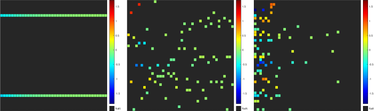
Figure 1:  An example of three space-time sampling regimes using the same number of samples. Here the $x$ axis denotes the time instances and the $y$ axis denotes the spatial values of evolving signals with colors representing the magnitude. Only values at colored spots are observed. 


The goal is to investigate the conditions on $\Omega$ to achieve stable recovery of the initial signal $\mathbf{x}_{0}$ from (possibly noisy) partial observations of states from a single trajectory $\{S_{\Omega_{\ell}}\mathbf{x}_{t_{\ell}}:\ell=0,1,\cdots,T-1\}$ and propose robust reconstruction strategies.




1.2 Summary of contributions


In this paper, we propose three random space-time sampling regimes to sample bandlimited graph diffusive fields. For each regime, we introduce a quantity called the spectral graph weighted coherence of order $(k,T)$. Such a quantity depends on the interplay between the sampling distribution and the localization of the bandlimited diffusion fields over the space-time locations. We provide sampling complexity bounds to ensure robust recovery of initial signal with high probability and show that they scale linearly with the square of spectral graph weighted coherence of order $(k,T)$. We show that temporal information can reduce the spatial sampling density and one can achieve comparable (even better) results given the same amount of space-time samples with the static case. We further provide a detailed comparison of three regimes in terms of their sample complexity and the influence of sampling probability distributions on the performance. More details are discussed in Section 4.3.


Finally, we propose a robust method to reconstruct any $k$-bandlimited signal from its noisy samples, with a detailed error analysis. The idea is to use an $\ell_{2}$ regularization term that utilizes the graph Laplacian and bandlimited property of the graph signals. The results show that our methods can recover $k$-bandlimited signals exactly in the absence of noise and the method is also robust to measurement acquisition noise and model errors. In addition, extensive numerical simulations are conducted on various graphs including an example of deblurring a real image from the space-time samples of its diffusion process, which further support our theoretical results and confirm that random dynamical sampling offers a robust alternative for the standard spatial sampling.


Note that our space-time sampling theorems are applicable to any dynamical system over the graph of the form $x_{t}=Ax_{t-1}$ with the evolution operator $A$ being a diagonalizable operator. For example, $A$ can be a polynomial function of any symmetrical Laplacian or adjacency matrix of any weighted undirected graph. It is also possible to generalize the current framework to bandlimited limited graph processes governed by a linear time-invariant system [22].


Nevertheless, the reconstruction methods proposed here are specifically designed to take advantage of the semi-definite positivity of the evolution operator. For simplicity and conciseness, we therefore concentrate on the normalized Laplacians.


Our work is built upon recent progress on sampling of bandlimited graph signals and dynamical sampling over regular domains. In particular, we generalize the work in [33] to bandlimited diffusion fields with three random-space sampling regimes. In Section 2, we give more detailed comparisons with these relevant works.



2 Related work



2.1 Dynamical sampling over regular domain


Previous work on dynamical sampling has focused on deterministic sampling over regular domains. Dynamical sampling was first proposed in [3, 2] by Aldroubi et al for linear time invariant systems, motivated by the pioneering work of [25] that considered the space-time sampling of bandlimited diffusion fields over the real line, see also [35, 18, 27, 28] for various extensions. The majority of the work [1, 8, 4, 6, 40, 43, 5, 23, 16] has focused on developing deterministic sampling theorems to ensure exact reconstruction, where the number and the location of sensors are fixed for successive time instances. Our paper is the first one to extend the dynamical sampling framework to graphs and consider the random space-time sampling regimes: the locations and numbers of sensors can change over time, and the observation time period is not necessarily successive. We will show that this allows us to adapt the graph topology to the sampling such that one needs much fewer number of space-time samples yet yields a more robust reconstruction.




2.2 Sampling and reconstruction of bandlimited graph signals


Sampling and reconstruction of bandlimited graph signals (corresponding to $T=1$ in our case) have been extensively studied and achieved remarkable progress. The existing approaches can be mainly categorized into selection sampling and aggregation sampling. In the first category, deterministic sampling (see e.g. [13, 10, 30, 31, 7, 21]) and random sampling scheme (see e.g. [14, 15, 20, 33]) were proposed. Using ideas of variable density sampling from compressed sensing, Vandergheynst et al. [33] derive random sampling schemes based on probability distributions over the graph vertexes. In this paper, we generalize their work to the bandlimited diffusion field and propose three different random space-time sampling schemes so that the work [33] becomes a special case of our regimes with $T=1$. In the second category, aggregation sampling aims to recover signals from (random weighted) linear combinations of signal values on a neighborhood of selected nodes. It corresponds to sampling a time-varying signal driven by a graph shift operator, whose matrix form has the same sparsity pattern with the adjacent matrix. The deterministic scheme proposed in [26] (see [45, 48] for extensions) can be viewed a special case of our regime 1 with a pre-selected set of nodes; the random scheme [44] used a graph shift operator with i.i.d. Gaussian entries, corresponding to the case of $T=2$ and observations are only made at $T=2$.


Compared to the static setting, there are relatively fewer work considering the sampling and reconstruction problem in dynamical system setting. Different models for the time series over graph have been proposed. The examples include distributed reconstruction algorithms for graph low-pass filtering processes [46] and batch reconstruction methods [34] for graph signals whose temporal difference is bandlimited.
[22] considered
both deterministic and Bernoulli random space-time sampling for bandlimited graph processes. Necessary conditions on probabilities are derived to ensure the exact reconstruction of the process and a convex optimization approach was proposed to choose the optimal sampling design. The proposed regime is most related to our regime 3. However, our work is different: we also consider regimes 1 and 2, and we use a different observation model by extending the idea of variable density sampling.



3 Preliminaries and Notation



3.1 Operators associated to graphs


We consider an undirected weighted graph $\mathcal{G}=(\mathcal{V},\mathcal{E},W)$ where $\mathcal{V}=\{v_{1},v_{2},\cdots,v_{n}\}$ is set of $n$ vertices and $\mathcal{E}\subset\mathcal{V\times V}$ is a set of edges. Let $\{v_{i},v_{j}\}$ denote the edge if $v_{i}$ and $v_{j}$ are connected. The weighted adjacent matrix $W$ is defined as




$$W(i,j)\triangleq\begin{cases}\alpha_{ij}&\mbox{if $\{v_{i},v_{j}\}\in\mathcal{E}$}\\
0&\mbox{otherwise}\end{cases};\alpha_{ij}\in\mathbb{R}_{+};\text{ for all }v_{i},v_{j}\in\mathcal{V}.$$





The weight associated with each edge in the graph often indicates similarity or dependency between the corresponding vertices. The connectivity and edge weights are dictated by the physics of the problem at hand, for instance, the weights are inversely proportional to the physical distance between nodes in the network. In particular, $W$ is symmetric. The degree $\deg(v_{i})$ of a vertex $v_{i}\in V$ is defined as $\deg(v_{i})=\sum_{j=1}^{n}W(i,j)$. ${D}:={\mathrm{diag}}(\deg(v_{i})_{i=1}^{n})$ denotes the diagonal degree matrix. In the following, we introduce important operators associated with the graph $\mathcal{G}$.



Definition 3.1.


The normalized diffusion operator of a graph $\mathcal{G}$ with weighted adjacent matrix ${W}\in\mathbb{R}^{n\times n}$ is defined by
$N={D}^{-\frac{1}{2}}W{D}^{-\frac{1}{2}}$. We call $N$ the diffusion matrix of $\mathcal{G}$. The normalized graph Laplacian operator is $L=I-N$.






3.2 Bandlimited graph signal


The matrix $L$ is real symmetric, and so it admits an eigen-decomposition ${L}=U\Sigma U^{\top}$ where the columns of $U\in\mathbb{R}^{n\times n}$ are orthonormal eigenvectors and the diagonal entries of $\Sigma$ consist of $n$ eigenvalues $\sigma_{1},\cdots,\sigma_{n}$. Furthermore, semi-definite positivity of $L$ implies that all eigenvalues are non-negative. Without loss of generality, we assume that $\sigma_{1}\leq\cdots\leq\sigma_{n}$. Note that $A=\exp(-\Delta tL)$, we have $A=U\Lambda U^{\top}$ with $\Lambda:=\exp(-\Delta t\Sigma)$. Let’s denote the diagonal entries of $\Lambda$ as $\lambda_{1}=\exp(-\Delta t\sigma_{1}),\cdots,\lambda_{n}=\exp(-\Delta t\sigma_{n})$. Thus we have $\lambda_{1}\geq\cdots\geq\lambda_{n}$.


In graph signal processing, the matrix $U$ is often viewed as the graph Fourier transform. For any signal $\mathbf{x}\in\mathbb{R}^{n}$ defined on the nodes of the graph $\mathcal{G}$, $\widehat{\mathbf{x}}=U^{\top}\mathbf{x}$ represents the Fourier coefficients of $\mathbf{x}$ ordered in increasing frequencies. The smooth graph signals are modelled as $k$ bandlimited signals: for $\mathbf{x}\in\mathbb{R}^{n}$ on $\mathcal{G}$ with bandwidth $k>0$ it satisfies
$\mathbf{x}=U_{k}\widehat{\mathbf{x}}^{k}$
where $\widehat{\mathbf{x}}^{k}:=\widehat{\mathbf{x}}(1:k)\in\mathbb{R}^{k}$ and
$U_{k}:=(\mathbf{u}_{1},\cdots,\mathbf{u}_{k})\in\mathbb{R}^{n\times k}$,
i.e., $U_{k}$ is the restriction of $U$ to its first $k$ vectors. This yields the following formal definition of a $k-$bandlimited signal.



Definition 3.2 (Bandlimited signal on $\mathcal{G}$).


A signal $\mathbf{x}\in\mathbb{R}^{n}$ defined on the nodes of the graph $\mathcal{G}$ is
$k$-bandlimited with $k\in\mathbb{N}\setminus\{0\}$ if $\mathbf{x}\in\mathrm{span}(U_{k})$.



Note that we use $U_{k}$ in our definition of $k$-bandlimited signals to handle the case where the eigen-decomposition is not unique.




3.3 Notation


In this work, capital letters are used for matrices, lower boldface letters for vectors, and regular letters for scalars. The set of the first $d$ natural numbers is denoted by $[d]$. For integers $i,n,T$, the notation $i:n:Tn$ stands for the set $\{k=i+jn\in[i,Tn]:\text{for some }j\in\mathbb{Z}\}$ and $I_{d}$ stands for the $d\times d$ identity matrix.


We let ${\mathrm{diag}}(\mathbf{x})$ denote the diagonal matrix with diagonal entries given by vector $\mathbf{x}$ and ${\mathrm{diag}}(X)={\mathrm{diag}}(X(1,1),\cdots,X(d,d))$ for $X\in\mathbb{R}^{d\times d}$.
Let $\mathbf{x}_{1},\cdots,\mathbf{x}_{t}$ be vectors and $X_{1},\cdots,X_{t}$ be matrices, we define ${\mathrm{diag}}(\mathbf{x}_{1};\cdots;\mathbf{x}_{t})$ and ${\mathrm{diag}}(X_{1};\cdots;X_{t})$ as the block diagonal matrix with
the $(i,i)$-th block of ${\mathrm{diag}}(\mathbf{x}_{1};\cdots;\mathbf{x}_{t})$ being ${\mathrm{diag}}(\mathbf{x}_{i})$ and the $(i,i)$-th block of ${\mathrm{diag}}(X_{1};\cdots;X_{t})$ being $X_{i}$ respectively.


Let $T$ be a positive integer and we define



(2)

$$f_{T}(\lambda)=\sqrt{\sum_{t=0}^{T-1}\lambda^{2t}},\;F_{k,T}={\mathrm{diag}}\left(\frac{1}{f_{T}(\lambda_{1})},\cdots,\frac{1}{f_{T}(\lambda_{k})}\right),\;\Lambda_{k}={\mathrm{diag}}(\lambda_{1},\cdots,\lambda_{k}).$$






4 Sampling of $k$-bandlimited diffusion fields


In this section, we describe three regimes that select a subset of space-time locations to sample a $k$-bandlimited diffusion field. Then, we prove that the corresponding space-time sampling procedure stably embeds the set of initial signals that consists of $k$-bandlimited signals. We describe how to reconstruct initial signals from the space-time samples in Section 5.



4.1 The space-time sampling procedure


To select the space-time sampling set $\Omega$, we introduce various probability distributions $\mathbf{p}$ serving as sampling distributions for three random regimes.



Definition 4.1.


The probability distributions can be defined as follows:


 

Random spatial locations at initial time: let $\mathbf{p}^{(1)}$ be a probability distribution on $[n]$. We define $P_{1}\in\mathbb{R}^{Tn\times Tn}$ as $P_{1}={\mathrm{diag}}({\mathbf{p}^{(1)};\cdots;\mathbf{p}^{(1)}})$.



 

Random spatial locations at consecutive times: let $\mathbf{p}_{t}^{(2)}$ be a probability distribution on $[n]$ describing sampling at time $t$, for all $t=0,1,\cdots,T-1$. The associated matrix $P_{2}\in\mathbb{R}^{Tn\times Tn}$ is defined as $P_{2}={\mathrm{diag}}(\mathbf{p}_{0}^{(2)};\cdots;\mathbf{p}_{T-1}^{(2)})$.



 

Random space-time locations: we let $\mathbf{p}^{(3)}$ be a probability distribution on $[Tn]$ and define $P_{3}\in\mathbb{R}^{Tn\times Tn}$ as $\mathrm{diag}(\mathbf{p}^{(3)})$.









We assume that the probability distributions above are all non-degenerate, i.e., entry-wise nonzero. Once the probability distributions are assigned, we obtain the nodes in the space-time sampling sets $\Omega$ independently (with replacement) according to the probability distributions. Note that $\Omega$ only needs to be selected once to sample all $k$-bandlimited diffusion fields over $\mathcal{G}$. After the sampling distributions and sampling set $\Omega$ are determined, we define the associated variables as follows.



Definition 4.2.


For three regimes, we define the associated sampling matrices and weighting matrices as follows.


 

Random spatial locations at initial time: $\Omega^{(1)}:=\Omega^{(1)}_{0}\times[T]$ where $\Omega^{(1)}_{0}=\{\omega_{1}^{(1)},\cdots,\omega_{m}^{(1)}\}$ is constructed by drawing $m$ indices independently (with replacement) from set $[n]$ according to probability $\mathbf{p}^{(1)}$, i.e.,
$\mathbb{P}(\omega_{j}^{(1)}=i)=\mathbf{p}^{(1)}(i),\text{ for all }j\in[m]\text{ and }i\in[n]$.
We define the sampling matrix



(3)

$$S_{1}={\mathrm{diag}}(\underbrace{S_{1}^{(0)};\cdots;S_{1}^{(0)}}_{T}),$$



where $S_{1}^{(0)}\in\mathbb{R}^{m\times n}$ is defined as
$S_{1}^{(0)}(i,j):=\begin{cases}1,&\text{ if }j=\omega_{i}\\
0,&\text{otherwise}\end{cases}$. Thus, we can define the probability matrix on the sampling set $P_{\Omega^{(1)}}=S_{1}P_{1}S_{1}^{\top}$.
To average the samples’ information at each time instance, we also introduce $M=Lm$ and the weighting matrix $W_{1}\in\mathbb{R}^{M\times M}$ as



(4)

$$W_{1}=\frac{1}{m}{\mathrm{diag}}(\underbrace{I_{m};\cdots;I_{m}}_{T}).$$






 

Random spatial locations at consecutive times: let $\Omega^{(2)}=\cup_{t=0}^{T-1}(\Omega_{t}^{(2)}\times\{t\})$ with $\Omega_{t}^{(2)}:=\{\omega_{t,1}^{(2)},\cdots,\omega_{t,m_{t}}^{(2)}\}$, where $\Omega_{t}^{(2)}$ is constructed by drawing $m_{t}$ indices independently (with replacement) from the set $[n]$ according to the probability distribution $\mathbf{p}_{t}^{(2)}$, i.e.,
$\mathbb{P}(\omega_{t,j}^{(2)}=i)=\mathbf{p}^{(2)}_{t}(i)$, for all $j\in[m_{t}]\text{ and }i\in[n]$.
We set $M=\sum_{t=0}^{T-1}m_{t}$ and define the sampling matrix $S_{2}\in\mathbb{R}^{M\times Tn}$ as



(5)

$$S_{2}={\mathrm{diag}}(S_{2}^{(0)};S_{2}^{(1)};\cdots;S_{2}^{(T-1)})$$



where $S_{2}^{(t)}\in\mathbb{R}^{m_{t}\times n}$ is defined as $S_{2}^{(t)}(i,j):=\begin{cases}1,&j=\omega_{t,i}^{(2)}\\
0,&\text{otherwise},\end{cases}$ for $t=0,\cdots,T-1$. Thus, we could define the probability matrix on the sampling set $P_{\Omega^{(2)}}=S_{2}P_{2}S_{2}^{\top}$.
To average the samples at each time instance, we define the weighting matrix $W_{2}\in\mathbb{R}^{M\times M}$ as



(6)

$$W_{2}={\mathrm{diag}}(\frac{1}{m_{0}}I_{m_{0}};\frac{1}{m_{1}}I_{m_{1}};\cdots;\frac{1}{m_{T-1}}I_{m_{T-1}}).$$






 

Random space-time locations: $\Omega^{(3)}:=\{\omega_{1}^{(3)},\cdots,\omega_{m}^{(3)}\}$ is constructed by drawing $m$ indices independently (with replacement) from $[Tn]$ according to probability distribution $\mathbf{p}^{(3)}$, i.e.,
$\mathbb{P}(\omega_{j}=i)=\mathbf{p}^{(3)}(i),\forall j\in[m]\text{ and }i\in[Tn]$.
For this sampling regime, we define the sampling matrix $S_{3}\in\mathbb{R}^{m\times Tn}$ as



(7)

$$S_{3}(i,j):=\begin{cases}1,&\text{ if }j=\omega_{i}^{(3}\\
0,&\text{otherwise}\end{cases},$$



the probability matrix on the sampling set $P_{\Omega^{(3)}}=S_{3}P_{3}S_{3}^{\top}$, and weighting matrix $W_{3}=\frac{1}{M}I_{M}$ with $M=m$.









4.2 Stable embedding of $k$-bandlimited signals via space-time samples


First let’s introduce a map
$\pi_{A,T}:\mathbb{R}^{n}\rightarrow\mathbb{R}^{Tn}$ that maps $k$-bandlimited signals to $k$-bandlimited diffusion fields and is defined by $\pi_{A,T}(\mathbf{x})=[\mathbf{x}^{\top},(A\mathbf{x})^{\top},\cdots,(A^{T-1}\mathbf{x})^{\top}]^{\top}$.
Notice that if $\mathbf{x}\in\mathrm{span}(U_{k})$, then $\pi_{A,T}(\mathbf{x})\in\mathrm{span}(\widetilde{U}_{k,T})$, where $\widetilde{U}_{k,T}\in\mathbb{R}^{Tn\times k}$ consists of orthonormal columns vectors and is defined below



(8)

$$\widetilde{U}_{k,T}=\begin{bmatrix}\frac{1}{f_{T}(\lambda_{1})}\mathbf{u}_{1}&\frac{1}{f_{T}(\lambda_{2})}\mathbf{u}_{2}&\cdots&\frac{1}{f_{T}(\lambda_{k})}\mathbf{u}_{k}\\
\frac{\lambda_{1}}{f_{T}(\lambda_{1})}\mathbf{u}_{1}&\frac{\lambda_{2}}{f_{T}(\lambda_{2})}\mathbf{u}_{2}&\cdots&\frac{\lambda_{k}}{f_{T}(\lambda_{k})}\mathbf{u}_{k}\\
\vdots&\vdots&\cdots&\vdots\\
\frac{\lambda_{1}^{T-1}}{f_{T}(\lambda_{1})}\mathbf{u}_{1}&\frac{\lambda_{2}^{T-1}}{f_{T}(\lambda_{2})}\mathbf{u}_{2}&\cdots&\frac{\lambda_{k}^{T-1}}{f_{T}(\lambda_{k})}\mathbf{u}_{k}\end{bmatrix}.$$



This observation implies that $\pi_{A,T}:\mathrm{span}(U_{k})\rightarrow\mathrm{span}(\widetilde{U}_{k,T})$. The following lemma shows that $\pi_{A,T}$ is a stable embedding and specifies lower and upper embedding constants.



Lemma 4.3.


For any $\mathbf{x}\in\mathrm{span}(U_{k})$, we have that




$$f_{T}(\lambda_{k})\|\mathbf{x}\|_{2}\leq\|\pi_{{A},T}(\mathbf{x})\|_{2}\leq f_{T}(\lambda_{1})\|\mathbf{x}\|_{2},$$



where the map $f_{T}$ is defined in (2).




The key observation that $\pi_{A,T}(\mathrm{span}(U_{k}))=\mathrm{span}(\widetilde{U}_{k,T})$ inspires us to interpret $k$-bandlimited diffusion fields as $k$-bandlimited signals over an extended space-time graph $\mathcal{G}_{T}$, whose top $k$ Laplacian eigenvectors are given by $\widetilde{U}_{k,T}$. Leveraging this interpretation, we connect the space-time sampling of bandlimited diffusion fields over $\mathcal{G}$ with the classical spatial sampling of $k$-bandlimited graph signals over $\mathcal{G}_{T}$.


Similar to compressed sensing, the number of space-time samples needed to guarantee stable reconstruction of $k$-bandlimited diffusion fields will depend on a quantity, the spectral graph weighted coherence of order $(k,T)$, that represents how the energy of bandlimited diffusion fields spreads over the space-time nodes. We will derive and understand this quantity via sampling on $\mathcal{G}_{T}$.


Let $\delta_{i}\in\mathbb{R}^{Tn}$ denote the Dirac at the space-time node $i$.
The quantity



(9)

$$\|\widetilde{U}_{k,T}(i,:)\|_{2}=\|\widetilde{U}_{k,T}^{\top}\delta_{i}\|_{2}$$



describes how much the energy of $\delta_{i}$ is concentrated on the first $k$ Fourier modes of $\mathcal{G}_{T}$, or equivalently, the distribution of the energy of the $k$-bandlimited diffusion fields over the space-time nodes.


When the quantity (9) is one, then there exist $k$-bandlimited diffusion fields whose energy is solely concentrated on the $i$th space-time node, and not sampling the $i$th node jeopardises the chance of reconstructions. When it is zero, then no $k$-bandlimited diffusion fields over $\mathcal{G}$ has a part of its energy on the $i$th node; one can safely remove this node from the sampling set. We thus see that the quality of our sampling method will depend on the interplay between the sampling distribution and the quantities $\|\widetilde{U}_{k,T}^{\top}\delta_{i}\|_{2}$ for $i\in[nT]$. Ideally, the larger $\|\widetilde{U}_{k,T}^{\top}\delta_{i}\|_{2}$ is, the higher probability of the node $i$ is observed. Below, we introduce the spectral graph weighted coherence of order $(k,T)$ to characterize the interplay between the sampling distribution for each regime and space-time nodes, where the case of $T=1$ corresponds to the graph weighted coherence introduced in [33, Definition 2.1] for the static case.



Definition 4.4 (Graph spectral weighted coherence of order $(k,T)$ $\mathbf{\nu}_{j,\mathbf{p}^{(j)}}^{k,T}$ ).


Let $\mathbf{p}^{(j)}$ represent a sampling distribution for $j=1,2,3$. The graph spectral weighted coherence $\mathbf{\nu}_{j,\mathbf{p}^{(j)}}^{k,T}$ of order $(k,T)$ for the triple $(\mathcal{G},T,\mathbf{p}^{(j)})$ is defined as following


 

Random spatial locations at the initial time:



(10)

$$\mathbf{\nu}_{1,\mathbf{p}^{(1)}}^{k,T}:=
\max_{1\leq i\leq n}\left\{\frac{1}{\sqrt{\mathbf{p}^{(1)}(i)}}\left\|\widetilde{U}_{k,T}((i:n:Tn),:)\right\|_{2}\right\},$$





where $\widetilde{U}_{k,T}((i:n:Tn),:)$ is the row submatrix of $\widetilde{U}_{k,T}$ with row indices in $(i:n:Tn)$



 

Random spatial locations at consecutive times:



(11)

$$\mathbf{\nu}_{2,\mathbf{p}^{(2)}}^{k,T}:=\begin{bmatrix}\mathbf{\nu}_{\mathbf{p}_{0}^{(2)}}\\
\vdots\\
\mathbf{\nu}_{\mathbf{p}_{T-1}^{(2)}}\end{bmatrix}=\begin{bmatrix}\max_{1\leq i\leq n}\frac{1}{\sqrt{\mathbf{p}_{0}^{(2)}(i)}}\|\widetilde{U}_{k,T}^{\top}\delta_{i}\|_{2}\\
\vdots\\
\max_{1\leq i\leq n}\frac{1}{\sqrt{\mathbf{p}_{T-1}^{(2)}(i)}}\|\widetilde{U}_{k,T}^{\top}\delta_{i+(T-1)n}\|_{2}\\
\end{bmatrix},$$






 

Random space-time locations: 



(12)

$$\mathbf{\nu}_{3,\mathbf{p}^{(3)}}^{k,T}:=\max_{1\leq i\leq Tn}\left\{\frac{1}{\sqrt{\mathbf{p}_{i}^{(3)}}}\|\widetilde{U}_{k,T}^{\top}\delta_{i}\|_{2}\right\},$$












From the definition, the spectral graph weighted coherence of order $(k,T)$ for each regime is thus a characterization of the interaction among the $k$-bandlimited signals, spectrum of the graph Laplacian, and the respective sampling distributions. For the ease of the readers, we summarize three sampling regimes in Table 4.1.





Sampling
①
②
③


Regimes


$\mathbf{p}^{(j)}$
$\mathbf{p}^{(1)}\in\mathbb{R}^{n}$
$\mathbf{p}^{(2)}=[\mathbf{p}_{0}^{(2)};\cdots;\mathbf{p}_{T-1}^{(2)}]\in\mathbb{R}^{n\times T}$
$\mathbf{p}^{(3)}\in\mathbb{R}^{Tn}$


$P_{j}$
$P_{1}={\mathrm{diag}}(\underbrace{\mathbf{p}^{(1)};\cdots;\mathbf{p}^{(1)}}_{T})$
$P_{2}={\mathrm{diag}}\left(\mathbf{p}_{0}^{(2)};\mathbf{p}_{1}^{(2)};\cdots;\mathbf{p}_{T-1}^{(2)}\right)$
$P_{3}={\mathrm{diag}}(\mathbf{p}^{(3)})$


$\Omega$
$\Omega^{(1)}=\Omega^{(1)}_{0}\times[T]$

$\Omega^{(2)}=\bigcup_{t=0}^{T-1}\Omega_{t}^{(2)}\times\{t\}$,

$\Omega^{(3)}=\{\omega_{1}^{(3)},\cdots,\omega_{m}^{(3)}\}$


$\Omega^{(1)}_{0}=\{\omega_{1}^{(1)},\cdots,\omega_{m}^{(1)}\}$

$\Omega_{t}^{(2)}=\{\omega_{t,1}^{(2)},\cdots,\omega_{t,m_{t}}^{(2)}\}$.



$S_{j}$

$S_{1}={\mathrm{diag}}(\underbrace{S_{1}^{(0)};\cdots;S_{1}^{(0)}}_{T})$,

$S_{2}={\mathrm{diag}}(S_{2}^{(0)};\cdots;S_{2}^{(T-1)})$
$S_{3}\in\mathbb{R}^{m\times Tn}$ with



$S_{1}^{(0)}\in\mathbb{R}^{m\times n}$ with


$S_{2}^{(t)}\in\mathbb{R}^{m_{t}\times n}$ with



$S_{1}^{(0)}(i,j)=\begin{cases}1,&j=\omega_{i}\\
0,&\text{otherwise}.\end{cases}$
$S_{2}^{(t)}(i,j)=\begin{cases}1,&j=\omega_{t,i}\\
0,&\text{otherwise}\end{cases}$
$S_{3}(i,j)=\begin{cases}1,&j=\omega_{i}\\
0,&\text{otherwise}.\\
\end{cases}$




for $t=0,\cdots,T-1$.




$P_{\Omega^{(j)}}$
$P_{\Omega^{(1)}}={\mathrm{diag}}(S_{1}P_{1}S_{1}^{\top})$
$P_{\Omega^{(2)}}={\mathrm{diag}}(S_{2}P_{2}S_{2}^{\top})$
$P_{\Omega^{(3)}}={\mathrm{diag}}(S_{3}P_{3}S_{3}^{\top})$


$W_{j}$
$W_{1}=\frac{1}{m}I_{mT}$
$W_{2}={\mathrm{diag}}(\frac{1}{m_{0}}I_{m_{0}};\cdots;\frac{1}{m_{T-1}}I_{m_{T-1}})$
$W_{3}=\frac{1}{m}I_{m}$


$\mathbf{\nu}_{j,\mathbf{p}^{(j)}}^{k,T}$

$\mathbf{\nu}_{1,\mathbf{p}^{(1)}}^{k,T}$ in (10)


$\mathbf{\nu}_{2,\mathbf{p}^{(2)}}^{k,T}$ in (11)


$\mathbf{\nu}_{3,\mathbf{p}^{(3)}}^{k,T}$ in (12)




Table 4.1: Relevant notations and matrices for different random space-time sampling regimes.




4.3 Properties of spectral graph weighted coherences


As shown later, the sampling size required to achieve stable embedding essentially depends on the spectral graph weighted coherence. Next we analyze its properties in Proposition 4.5.



Proposition 4.5.


We list several properties of the spectral graph weighted coherences of order $(k,T)$ that are useful for later analysis.




 

For any probability distribution $\mathbf{p}^{(j)}$ for $j=1,2,3$, we have that




 

$\left(\mathbf{\nu}_{1,\mathbf{p}^{(1)}}^{k,T}\right)^{2}\geq\sum_{i=1}^{n}\left\|\widetilde{U}_{k,T}((i:n:Tn),:)\right\|_{2}^{2}\geq k$ and the first inequality becomes an equality when



(13)

$$\mathbf{p_{opt}}^{(1)}(i)=\frac{\left\|\widetilde{U}_{k,T}((i:n:Tn),:))\right\|_{2}^{2}}{\sum_{\ell=1}^{n}\left\|\widetilde{U}_{k,T}((\ell:n:Tn),:)\right\|_{2}^{2}}\quad\text{ for }i=1,\cdots,n.$$






 

$(\nu_{2,\mathbf{p}^{(2)}}^{k,T}(t))^{2}\geq\sum\limits_{\ell=1}^{k}\frac{\lambda_{\ell}^{2t}}{f_{T}^{2}(\lambda_{\ell})}$ for $t=0,\cdots,T-1$ and the equality holds when



(14)

$$\mathbf{p_{t,opt}}^{(2)}(i)=\frac{\|\widetilde{U}_{k,T}^{\top}\delta_{i+tn}\|_{2}^{2}}{\sum_{\ell=1}^{k}\lambda_{\ell}^{2t}/f_{T}^{2}(\lambda_{\ell})}.$$



As a result,
$\sum_{t=1}^{T}\left(\nu_{2,\mathbf{p}^{(2)}}^{k,T}(t)\right)^{2}\geq k$.



 

$\left(\mathbf{\nu}_{3,\mathbf{p}^{(3)}}^{k,T}\right)^{2}\geq k$ and the equality holds when



(15)

$$\mathbf{p_{opt}}^{(3)}(i)=\frac{\|\widetilde{U}_{k,T}^{\top}\delta_{i}\|_{2}^{2}}{k}$$









 

For any sampling distributions, we have that




$$T\left(\nu_{1,\mathbf{p}^{(1)}}^{k,T}\right)^{2}\geq\left(\nu_{3,\mathbf{p}^{(3)}}^{k,T}\right)^{2}\geq\sum_{t=0}^{T-1}\left(\nu_{2,\mathbf{p}^{(2)}}^{k,T}(t)\right)^{2}.$$



In particular, we call the probability defined in (13), (14) and (15) the optimal distribution for the regime 1,2 and 3. In this case, we have




$$T\left(\nu_{1,\mathbf{p}^{(1)}}^{k,T}\right)^{2}\geq\left(\nu_{3,\mathbf{p}^{(3)}}^{k,T}\right)^{2}=\sum_{t=0}^{T-1}\left(\nu_{2,\mathbf{p}^{(2)}}^{k,T}(t)\right)^{2}=k.$$










We are now ready to present the main theorem in this section. We represent three random space-time sampling procedures of $k$-bandlimited diffusion fields as three operators $P_{\Omega^{(j)}}^{-\frac{1}{2}}W_{j}^{\frac{1}{2}}S_{j}$ for $j=1,2,3$. We provided a unified theory to show that their composition with the map $\pi_{A,T}$ yields stable embeddings of $k$-bandlimited signals with high probability, as long as the number of space-time samples taken is above a threshold depending on the respective spectral graph coherence.



Theorem 4.6.


Let $P_{\Omega^{(j)}},S_{j},W_{j}$ be defined in Table 4.1 with the sampling distribution $\mathbf{p}^{(j)}$.
For any $\delta,\epsilon\in(0,1)$, the following inequality



(16)

$$(1-\delta)f_{T}^{2}(\lambda_{k})\|\mathbf{x}\|^{2}\leq\|P_{\Omega^{(j)}}^{-\frac{1}{2}}W_{j}^{\frac{1}{2}}S_{j}\pi_{A,T}(\mathbf{x})\|_{2}^{2}\leq(1+\delta)f_{T}^{2}(\lambda_{1})\|\mathbf{x}\|_{2}^{2},$$



holds with probability at least $1-\epsilon$,
provided that $m\geq\frac{3}{\delta^{2}}\left(\mathbf{\nu}_{j,\mathbf{p}^{(j)}}^{k,T}\right)^{2}\log\left(\frac{2k}{\epsilon}\right)$ for $j=1,3$, and $m_{t}\geq\frac{3}{\delta^{2}}\left(\mathbf{\nu}_{2,\mathbf{p}^{(2)}}^{k,T}(t)\right)^{2}\log\left(\frac{2k}{\epsilon}\right)$ for $j=2$, where $m_{t}$ is the number of space-time samples taken at time $t$.




(16) represents the stable embedding of $k$-bandlimited signals into $\mathbb{R}^{m}$. Let us take two different vectors $\mathbf{x}_{1}\neq\mathbf{x}_{2}$ in $\mathrm{span}(U_{k})$. Notice that $\mathbf{x}_{1}-\mathbf{x}_{2}\in\mathrm{span}(U_{k})$, then $\|P_{\Omega^{(j)}}^{-\frac{1}{2}}W_{j}^{\frac{1}{2}}S_{j}\pi_{A,T}(\mathbf{x}_{1}-\mathbf{x}_{2})\|_{2}^{2}\geq(1-\delta)f_{T}^{2}(\lambda_{k})\|\mathbf{x}_{1}-\mathbf{x}_{2}\|^{2}>0.$



Remark 4.7.


We make several important comments on Theorem 4.6.


 

In the case of $T=1$, $f_{T}^{2}(\lambda_{1})=f_{T}^{2}(\lambda_{k})=1$ and all the spectral graph weighted coherences equal to $(\nu_{\mathbf{p}}^{k})^{2}=\max_{1\leq i\leq n}\frac{\|U_{k}^{\top}\delta_{i}\|^{2}_{2}}{\mathbf{p}(i)}$, which coincides with [33,  Theorem 2.2], that the embedding operator satisfies the Restricted Isometry Property (RIP). Note that for regime 1, the total number of space-time samples is $Tm$ and our analysis in Proposition 4.5 shows that
$T(\nu_{1,\mathbf{p}^{(1)}}^{k,T})^{2}$ is the largest among three regimes. Even in this case, due to the temporal dynamics, one would expect fewer requirements of spatial sensors than the static case: Indeed, one can verify that $\left(\nu_{1,\mathbf{p}^{(1)}}^{k,T}\right)^{2}\leq\left(\nu_{\mathbf{p}}^{k}\right)^{2}$.
We also refer to the numerical section (Section 6) for more empirical evidences.



 

In practical situations, one just needs to measure the bandlimited diffusion fields by $S_{j}\pi_{A,T}(\mathbf{x})$. The re-weighting by
$P_{\Omega^{(j)}}^{-\frac{1}{2}}W_{j}^{\frac{1}{2}}$ can be done offline.



 

The spectral graph weighted coherences $(\mathbf{\nu}_{j,\mathbf{p}^{(j)}}^{k,T})^{2}\geq k$ for $j=1,3$ and $\sum_{t=1}^{T}(\mathbf{\nu}_{j,\mathbf{p}^{(2)}}^{k,T})^{2}(t)\geq k$ (see Proposition 4.5). It indicates that, we need to have at least $k$ space-time samples in all three regimes. Note that $k$ is also the minimum number of measurements that one must take to ensure the reconstruction of the $k$ bandlimited signals. Furthermore, the optimal spectral graph weighted coherence for regimes 2 and 3 is $k$ and therefore is independent of the total sampling time. This indicates that, one can expect to use fewer number of spatial sensors at each time instance on average as $T$ increase without hurting too much reconstruction accuracy, we refer to Theorem 5.1.



 

By part (b) of Proposition 4.5, the sampling complexity bounds satisfy that regime 1 $\geq$ regime 3 $\geq$ regime 2. This is consistent with our numerical results in Section 6.







Theorem 4.6 generalizes the well-known compressed sensing results in bounded orthonormal systems to the sampling of bandlimited diffusion fields with various space-time sampling regimes. Here we are in a different setting where the signal model is the bandlimited diffusion field. We leverage this temporal structure to connect with the orthonormal matrix $\widetilde{U}_{k,T}$. This connection allows us to utilize the same concentration inequalities used in compressed sensing yet refine and tighten the space-time sampling conditions.


In part $(a)$ of Proposition 4.5, we derive $\mathbf{p}_{\textbf{opt}}^{(j)}$for regime $j$, that minimizes the corresponding $\nu_{j,\mathbf{p}^{(j)}}^{k,T}$. Combining Theorem 4.6 and part $(a.2)$, part $(a.3)$ of Proposition 4.5, we can see that there always exists a sampling distribution for regime 2 and regime 3 such that $\mathcal{O}(k\log k)$ space-time samples are enough to capture all $k$-bandlimited signals. For regime 1, due to the inequality in part $(a.1)$, one would expect more space-time samples than other two regimes.




4.4 Intuitive links between graph diffusion process and the spectral graph weighted coherence


We will interpret $i\in[nT]$ as a space-time node in $[n]\times[T]$. We give here some examples showing how the spectral graph weighted coherence changes for diffusion processes over different graphs.


Consider circulant graphs with periodic boundary conditions, whose adjacent matrices are real and symmetric circulant matrices. In this case, the eigenvectors of their Laplacian are the $n$ dimensional classical Fourier modes. For simplicity, assume that the top $k$ eigenvalues are distinct. Let $\lambda_{1},\lambda_{2},\cdots,\lambda_{k}$ denote the eigenvalues of evolution operator $A$ for the heat diffusion process.  In this case, one can show that $\mathbf{p_{opt}}^{(1)}$ is the uniform distribution, and $\mathbf{p_{opt}}^{(2)}$ and $\mathbf{p_{opt}}^{(3)}$ have the identical components for a fixed time instance. These conclusions come from the following two facts:

(i)For regime 1, $\left\|\widetilde{U}_{k,T}((i:n:Tn),:)\right\|_{2}$ is the same for all $1\leq i\leq n$ and it equals to the operator norm of the matrix




$$\frac{1}{\sqrt{n}}\begin{bmatrix}1&1&\cdots&1\\
\lambda_{1}&\lambda_{2}&\cdots&\lambda_{k}\\
\vdots&\vdots&\cdots&\vdots\\
\lambda_{1}^{T-1}&\lambda_{2}^{T-1}&\cdots&\lambda_{k}^{T-1}\end{bmatrix}\begin{bmatrix}{1}/{f_{T}(\lambda_{1})}&0&\cdots&0\\
0&{1}/{f_{T}(\lambda_{2})}&\cdots&0\\
\vdots&\vdots&\cdots&\vdots\\
0&0&\cdots&{1}/{f_{T}(\lambda_{k})}\end{bmatrix}.$$



(ii) For regime 2 and regime 3, $\left\|\widetilde{U}_{k,T}^{\top}\delta_{i}\right\|_{2}$ is the same for all node $i$ at the time instance $t$ and it equals to
$\frac{1}{\sqrt{n}}\sqrt{\sum_{j=1}^{k}{\lambda_{j}^{2(t-1)}}/{f_{T}(\lambda_{j})^{2}}}$.


Let us consider the graph made of $k$ disconnected components of size $n_{1},\cdots,n_{k}$ such that $\sum_{i=1}^{k}n_{i}=n$. Let the Laplacian $L$ be the graph Laplacian with edge weights all equal to one. Then a basis of $\mathrm{span}(U_{k})$ is the concatenation of the square root of the degree operator times the indicator vectors of each component. Moreover, $\mathrm{span}(U_{k})$ is the eigenspace associated to the eigenvalue 0 of $L$. So the heat diffusion process over this eigenspace is the trivial identity. So the temporal dynamics play no role in sampling and it will be the same with the static case. By calculation, for the node $i$ at component $j$, we have




$$\left\|\widetilde{U}_{k,T}((i:n:Tn),:)\right\|_{2}=\frac{\sqrt{d_{ij}}}{\sqrt{d_{j}}}~{}\text{ and }~{}\left\|\widetilde{U}_{k,T}^{\top}\delta_{i}\right\|_{2}=\frac{\sqrt{d_{ij}}}{\sqrt{d_{j}T}},$$



where $d_{ij}$ is the degree of node $i$ and $d_{j}$ is the total degree of nodes in component $j$.


To keep things simplified, let us assume each component is regular, i.e., each node has the same degree. In this case, in $\mathbf{p_{opt}}^{(1)}$, the probability of choosing the spatial node $1\leq i\leq n$ at component $j$ is $\frac{1}{kn_{j}}$, coinciding with the case $T=1$. For regime 2 and 3, the optimal probability of choosing the spatial node $i$ at time $t$ is $\frac{1}{k{n_{j}}}$ and $\frac{1}{k{n_{j}T}}$ respectively. Thus, if all components have the same size, then uniform sampling is the optimal sampling. If the components have different sizes, the smaller a component is, the larger the probability of sampling one of its nodes is. We can see that optimal sampling requires that each component is sampled with probability $\frac{1}{k}$, independent of its size. The probability that each component is sampled at least once, a necessary condition for perfect recovery, is thus higher than that using uniform sampling. In the numerical section (Section 6), we consider the loosely defined
community-structured graph, which is a relaxation of the strictly disconnected component example. In this case, one also expects that $\mathbf{p}_{\textbf{opt}}^{(j)}$ to sample a node is inversely proportional to the size of its community.



5 Reconstruction of $k$-bandlimited signals from space-time samples


In this section, we are interested in designing a robust procedure to recover the initial signal in $\mathrm{span}(U_{k})$ from $M$ space-time samples. Specifically,
the space-time samples $\mathbf{y}\in\mathbb{R}^{M}$ are defined as




$$\mathbf{y}=S_{j}(\pi_{A,T}(\mathbf{x}))+\mathbf{e}$$



where $\mathbf{e}\in\mathbb{R}^{M}$ models the observational noise and $S_{j}$ is defined in Definition 4.2.


When one knows a basis for $\mathrm{span}(U_{k})$, we adopt the standard least squares method to estimate $\mathbf{x}\in\text{span}(U_{k})$ from $\mathbf{y}$. This is done by solving



(17)

$${\mathbf{x}}^{*}=\arg\min_{\widetilde{\mathbf{x}}\in\text{span}({U}_{k})}\|P_{\Omega^{(j)}}^{-1/2}W_{j}^{\frac{1}{2}}(S_{j}\pi_{A,T}(\widetilde{\mathbf{x}})-\mathbf{y})\|_{2}.$$



Here we introduce the weighting matrix $P_{\Omega^{(j)}}^{-1/2}W_{j}^{\frac{1}{2}}$ in (17) to ensure the stable embedding property in Theorem 4.6. The solution to (17) is obtained by solving






$$\mathrm{z}=\arg\min_{\widetilde{\mathrm{z}}\in\mathbb{R}^{k}}\|P_{\Omega^{(j)}}^{-1/2}W_{j}^{\frac{1}{2}}(S_{j}\pi_{A,T}U_{k}(\widetilde{\mathbf{z}})-\mathbf{y})\|_{2}$$



and setting ${\mathbf{x}}^{*}=U_{k}\mathbf{z}$. We generalize the idea of [33, Theorem 3.1] to prove that ${\mathbf{x}}^{*}$ is a faithful estimation of $\mathbf{x}$ so that [33, Theorem 3.1] becomes a special case of the following theorem:



Theorem 5.1.


Let $\Omega^{(j)}$ be a sampling set according to a sampling distribution $\mathbf{p}^{(j)}$, and $S_{j}$ be the sampling matrix associated to $\Omega^{(j)}$. Let $\varepsilon,\delta\in(0,1)$ and suppose that $m\geq\frac{3}{\delta^{2}}(\nu_{j,\mathbf{p}^{(j)}}^{k,T})^{2}\log(\frac{2k}{\varepsilon})$ for $j=1,3$ or $m_{t}\geq\frac{3}{\delta^{2}}(\nu_{2,\mathbf{p}^{(2)}}^{k,T}(t))^{2}\log(\frac{2k}{\varepsilon})$ for $j=2$. With probability at least $1-\varepsilon$, the following holds for all $\mathbf{x}\in\text{span}({U}_{k})$ and all $\mathbf{e}\in\mathbb{R}^{M}$.


 

Let ${\mathbf{x}}^{*}$ be the solution of Problem (17) with $\mathbf{y}=S_{j}(\pi_{A,T}(\mathbf{x}))+\mathbf{e}$. Then



(18)

$$\|\mathbf{x}^{*}-\mathbf{x}\|_{2}\leq\frac{2}{\sqrt{1-\delta}f_{T}(\lambda_{k})}\|P_{\Omega^{(j)}}^{-1/2}W_{j}^{\frac{1}{2}}\mathbf{e}\|_{2},$$



where $f_{T}$ is defined in (2)



 

There exist particular vectors $\mathbf{e}_{0}\in\mathbb{R}^{M}$ such that the solution ${\mathbf{x}}^{*}$ of Problem (17) with $\mathbf{y}=S_{j}\pi_{A,T}(\mathbf{x})+\mathbf{e}_{0}$ satisfies



(19)

$$\|\mathbf{x}^{*}-{\mathbf{x}}\|_{2}\geq\frac{1}{\sqrt{1+\delta}f_{T}(\lambda_{1})}\|P_{\Omega^{(j)}}^{-1/2}W_{j}^{\frac{1}{2}}\mathbf{e}_{0}\|_{2}.$$










The estimate (18) tells us that if $\mathbf{e}=0$, then ${\mathbf{x}}^{*}=\mathbf{x}$ with high probability. In the presence of noise, (18) shows that $\|\mathbf{x}^{*}-{\mathbf{x}}\|_{2}$ scales linearly with $\|P_{\Omega^{(j)}}^{-1/2}W_{j}^{\frac{1}{2}}\mathbf{e}\|_{2}$, and the estimate (19) shows that the bound on $\|\mathbf{x}^{*}-{\mathbf{x}}\|_{2}$ is sharp up to a constant. In the case of uniform sampling, we have



(20)

$$\|P_{\Omega^{(j)}}^{-1/2}W_{j}^{\frac{1}{2}}\mathbf{e}\|_{2}^{2}
=
{\frac{nT}{M}}\|\mathbf{e}\|_{2}^{2},j=1,3$$





(21)

$$\|P_{\Omega^{(2)}}^{-1/2}W_{2}^{\frac{1}{2}}\mathbf{e}\|_{2}^{2}
=
\sum_{t=0}^{T-1}\frac{n}{m_{t}}\|\mathbf{e}_{t}\|_{2}^{2},$$





where $\mathrm{e}_{t}$ denotes the projection of $\mathrm{e}$ into the components at time instance $t$.


In the case of non-uniform sampling, the noise may be amplified a lot at some particular draws of $\Omega$ due to some probability weights could be very close to 0. Non-uniform sampling could thus be very sensitive to noise unlike uniform sampling. Fortunately, this is a worst case scenario and it is unlikely to draw samples from locations where the probability is small by our sampling procedures. For each regime, the expectation $\mathbb{E}\|P_{\Omega^{(j)}}^{-1/2}W_{j}^{\frac{1}{2}}\mathbf{e}\|_{2}^{2}$ over the choice of $\Omega^{(j)}$
is as in the right hand side of (20) and (21) respectively. Therefore the noise term is not too large on average over the draw of $\Omega$.


Notice that to solve (17), we need to know $U_{k}$ in advance, which could be computationally expensive for large scale graphs. When $U_{k}$ is not given, we propose to estimate $\mathbf{x}$ by solving the following regularized least square problem



(22)

$$\min_{\widetilde{\mathbf{x}}\in\mathbb{R}^{n}}\|P_{\Omega^{(j)}}^{-1/2}W_{j}^{\frac{1}{2}}(S_{j}\pi_{A,T}(\widetilde{\mathbf{x}})-\mathbf{y})\|_{2}^{2}+\gamma\widetilde{\mathbf{x}}^{\top}g(L)\widetilde{{\mathbf{x}}},$$



where $\gamma>0$ and $g:\mathbb{R}\rightarrow\mathbb{R}$ is a nonnegative and nondecreasing polynomial function. One can find a solution to (22) by solving the following equation




$$(\pi_{A,T}^{\top}S_{j}^{\top}W_{j}^{\frac{1}{2}}P_{\Omega^{(j)}}^{-1}W_{j}^{\frac{1}{2}}S_{j}\pi_{A,T}+\gamma g(L)){\mathbf{x}}=\pi_{A,T}^{\top}S_{j}^{\top}W_{j}^{\frac{1}{2}}P_{\Omega^{(j)}}^{-1}W_{j}^{\frac{1}{2}}\mathbf{y}.$$





The idea of this relaxation comes from graph-filtering techniques which have found connections with decoders used in the semi-supervised learning on graphs [33]. In our problem, we use the penalty term $\gamma\widetilde{\mathbf{x}}^{\top}g(L)\widetilde{\mathbf{x}}$ to incorporate the smoothness of initial signal. The next theorem provides bounds for the error between the original signal $\mathbf{x}$ and the solution of (22), where [33, Theorem 3.2] becomes a special case for $T=1$.



Theorem 5.2.


Let $\Omega^{(j)}$ be a sampling set which obtained according to the sampling distribution $\mathbf{p}^{(j)}$. $P_{\Omega^{(j)}}$, $S_{j}$, $W_{j}$ are provided in Table 4.1 associated with $\mathbf{p}^{(j)}$.
$M_{\max}>0$ is a constant such that $\|P_{\Omega^{(j)}}^{-1/2}W_{j}^{\frac{1}{2}}S_{j}\|_{2}\leq M_{\max}$. Let $\varepsilon,\delta\in(0,1)$ and suppose that $m\geq\frac{3}{\delta^{2}}(\nu_{j,\mathbf{p}^{(j)}}^{k,T})^{2}\log(\frac{2k}{\varepsilon})$ for $j=1,3$ (and $m_{t}\geq\frac{3}{\delta^{2}}\left(\mathbf{\nu}_{2,\mathbf{p}^{(2)}}^{k,T}(t)\right)^{2}\log(\frac{2k}{\varepsilon})$ for $j=2$). With probability at least $1-\varepsilon$, the following holds for all $\mathbf{x}\in\text{span}({U}_{k})$ and all $\mathbf{e}\in\mathbb{R}^{M}$, all $\gamma>0$, and all nonnegative and nondecrasing polynomial functions $g$ such that $g(\sigma_{k+1})>0$, where $\sigma_{k+1}$ is the ($k+1$)th singular value of $L$.


Let $\mathbf{x}^{*}$ be the solution of Problem (22) with $\mathbf{y}=S_{j}(\pi_{A,T}(\mathbf{x}))+\mathbf{e}$. Then



(23)


$$\|\alpha^{*}-\mathbf{x}\|_{2}\leq\frac{1}{\sqrt{1-\delta}f_{T}(\lambda_{k})}\left(2+\frac{M_{\max}f_{T}(\lambda_{k+1})}{\sqrt{\gamma g(\sigma_{k+1})}}\right)\|P_{\Omega^{(j)}}^{-1/2}W_{j}^{\frac{1}{2}}\mathbf{e}\|_{2}+$$





$$\frac{1}{\sqrt{1-\delta}f_{T}(\lambda_{k})}\left(M_{\max}f_{T}(\lambda_{k+1})\sqrt{\frac{g(\sigma_{k})}{g(\sigma_{k+1})}}+\sqrt{\gamma g(\sigma_{k})}\right)\|\mathbf{x}\|_{2}$$




and



(24)

$$\|\beta^{*}\|_{2}\leq\frac{1}{\sqrt{\gamma g(\sigma_{k+1})}}\|P_{\Omega^{(j)}}^{-1/2}W_{j}\mathbf{e}\|_{2}+\left(\sqrt{\frac{g(\sigma_{k})}{g(\sigma_{k+1})}}\|\mathbf{x}\|_{2}\right),$$



where $\alpha^{*}:=U_{k}U_{k}^{\top}\mathbf{x}^{*}$, $\beta^{*}:=(I_{n}-U_{k}U_{k}^{\top})\mathbf{x}^{*}$ and $f_{T}$ is defined in (2).




Notice that when $T=1$, the bounds in Theorem 5.2 are exactly the bounds in [33, Theorem 3.2], due to that $f_{T}(\lambda_{k})=f_{T}(\lambda_{k+1})=1$ and $W_{j}=\frac{1}{m}I_{n}$.
In the estimates, $x^{*}=\alpha^{*}+\beta^{*}$.
To find a bound for $\|x^{*}-x\|_{2}$, one could simply use the triangular inequality and the bounds in (23), (24).


In the absence of noise, we thus have




$$\|x^{*}-x\|_{2}\leq\left(\left(\frac{M_{\max}f_{T}(\lambda_{k+1})}{\sqrt{1-\delta}f_{T}(\lambda_{k})}+1\right)\sqrt{\frac{g(\sigma_{k})}{g(\sigma_{k+1})}}+\frac{\sqrt{\gamma g(\sigma_{k})}}{\sqrt{1-\delta}f_{T}(\lambda_{k})}\right)\|\mathbf{x}\|_{2}.$$



If $g(\sigma_{k})=0$, we notice that we obtain a perfect reconstruction. Note that $g$ is supposed to be nondecreasing and nonnegative. In addition $\sigma_{1}\leq\cdots\leq\sigma_{n}$. Thus $g(\sigma_{k})=0$ implies that we also have $g(\sigma_{1})=\cdots=g(\sigma_{k-1})=0$. If $g(\sigma_{k})\neq 0$, the above bound shows that we should choose $\gamma$ as close as possible to $0$ and seek to minimize the ratio $\frac{g(\sigma_{k})}{g(\sigma_{k+1})}$ to minimize the upper bound on the reconstruction error. Notice that if $g(L)=L^{\ell}$ for $\ell\in\mathbb{N}^{*}$, then the ratio $g(\sigma_{k})/g(\sigma_{k+1})$ decreases as $\ell$ increases. Thus increasing the power of $L$ and taking $\gamma$ sufficiently small to compensate the potential growth of $g(\sigma_{k})$ is a simple solution to improve the reconstruction quality in the absence of noise. In addition, notice that $f_{T}$ is an increasing function with respect to $T$ (see (2)). Thus $1/f_{T}(\lambda_{k})$ will be decreasing as $T$ is increasing. Additionally, $\lambda_{k}\geq\lambda_{k+1}$, we have that $f_{T}(\lambda_{k+1})/f_{T}(\lambda_{k})$ is a nonincreasing function with respect to $T$. Therefore, for fixed $g$, the error bound will be a nonincreasing function with respect to $T$.


In the presence of noise, for a fixed function $g$, the upper bound on the reconstruction error is minimized for a value of $\gamma$ proportional to $\|P_{\Omega^{(j)}}W_{j}\mathbf{e}\|_{2}/\|\mathbf{x}\|_{2}$. To optimize the result further, one should seek to have $g(\sigma_{k})$ as small as possible and $g(\sigma_{k+1})$ as large as possible.


Therefore, the reconstruction of the original bandlimited graph signal can be summarized in Algorithm 1.


Algorithm 1   Procedure to reconstruct the original signal


1:  Input:  The signal evolution operator ${A}\in\mathbb{R}^{n\times n}$, the samples $\{\mathbf{y}_{t}^{(j)}\}_{t=0}^{T-1}$, sampling sets $\Omega^{(j)}$, and the probability distributions $\mathbf{p}^{(j)}$.



2:  Generate the sampling matrix $S_{j}$, the weighting matrix $W_{j}$ from the sampling set $\Omega^{(j)}$ and matrix $P_{j}$ from the probability distribution $\mathbf{p}^{(j)}$.



3:  Stack the samples together to a column vector and denote it as $\mathbf{y}^{(j)}$



4:  if The support $U_{k}$ of $\mathbf{x}$ is known then





5:     Set ${\mathbf{x}}^{*}=\arg\min\limits_{\widetilde{\mathbf{x}}\in\text{span}({U}_{k})}\|P_{\Omega^{(j)}}^{-1/2}W_{j}^{\frac{1}{2}}(S_{j}\pi_{A,T}(\widetilde{\mathbf{x}})-\mathbf{y})\|_{2}$ as estimate of $\mathbf{x}$.



6:  else




7:     Choose some constant $\gamma$ and regularizization function $g(z)$.



8:     Set ${\mathbf{x}}^{*}=\arg\min\limits_{\widetilde{\mathbf{x}}\in\mathbb{R}^{n}}\|P_{\Omega^{(j)}}^{-1/2}W_{j}^{\frac{1}{2}}(S_{j}\pi_{A,T}(\widetilde{\mathbf{x}})-\mathbf{y})\|_{2}^{2}+\gamma\widetilde{\mathbf{x}}^{\top}g(L)\widetilde{\mathbf{x}}$ as estimate of $\mathbf{x}$.



9:  end if


10:  Output: $\mathbf{x}^{*}$. 






6 Numerical Experiments









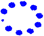
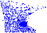
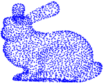
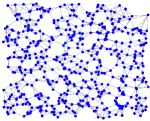
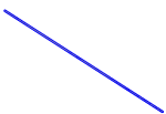
Figure 2:  The five different graphs used in the simulations: the figures are community graph, Minnesota graph, bunny graph, sensor graph and ring graph from left to right.


In this section, we empirically illustrate the theoretical findings and demonstrate the performance of the proposed algorithms.


Graphs


We use almost the same set of graphs in [33]. It consists of five different types of graphs, and is all available in the GSP toolbox [29] which is presented in Fig. 2: a) different community-type graphs of size $V=1000$; b)Minnesota road graph of size $V=2642$; c) Stanford bunny graph of size $V=2503$; d) an unweighted sensor graph of size $V=1000$ ; e) a path graph of size $V=1000$. Each node
is connected to its left and right neighbours except for the
boundary nodes which only have one neighbour.



Heat diffusion processes


We use the normalized Laplacian $L$ and consider the continuous heat diffusion processes over the graphs in all experiments with the evolution operator $A=\exp(-\Delta tL)$. Note that in [33], the combinatorial Laplacian was used, so we also run the experiments for $T=1$ for comparison with static case, instead of using the numerical results in [33]. The specific parameters are summarized in Table 6.1.





Type
Community
Minesota
Bunny
Sensor
Path
Real images




$\Delta t$
4
30
30
10
4
1


$T$
20
20
20
10
20
6



Table 6.1:  Parameters in heat diffusion processes 



Space-time sampling


All space-time
samples are taken with replacement as stated in Theorem 4.6. The total number of space-time samples is denoted by $M$ and $m_{t}$ for $t=0,\cdots,T-1$ are set to be equal for regime 2.




6.1 Effect of the space-time sampling distributions on $M$



First we show how $\mathbf{p}^{(j)}$ on the proposed sampling regimes
affect the required total number of samples $M$ to ensure stable embedding (16).
We compute the lower embedding constant




$$\small\underline{\delta}_{k,\mathbf{p}^{(j)}}:
=\min_{x\in\mathrm{span}(U_{k}),\|x\|=1}\|P_{\Omega^{(j)}}^{-\frac{1}{2}}W_{j}^{\frac{1}{2}}S_{j}\pi_{A,T}(\mathbf{x})\|_{2}^{2}$$






$$=\lambda_{\text{min}}(U_{k}^{\top}\pi_{A,T}^{\top}S_{j}^{\top}W^{\frac{1}{2}}P_{\Omega^{(j)}}^{-1}W^{\frac{1}{2}}S_{j}\pi_{A,T}U_{k})\vspace{-1mm}$$



for different $M$. We compute $\underline{\delta}_{k,\mathbf{p}^{(j)}}$ for 250 independent draws of the matrices $S_{j}$s.



6.1.1 Using community graphs


Inspired by [33], we use three types of community graphs, denoted by $C_{1},C_{2},C_{3}$, to study the effect of the size of the communities on sampling distributions. All these graphs have $10$ communities with $9$ of them of approximately equal size and the last community being reduced size. Specifically: (i) the graphs of type $C_{1}$ have $10$ communities of size $100$; (ii) the graphs of type $C_{2}$ have $1$ community of size $25$, $8$ communities of size $108$, and $1$ community of size $111$;
(iii) the graphs of type $C_{3}$ have $1$ community of size $13$, $8$ communities of size $109$, and $1$ community of size $115$.




$\underline{\delta}_{10,\pi^{(1)}}$



$\underline{\delta}_{10,\pi^{(2)}}$



$\underline{\delta}_{10,\pi^{(3)}}$







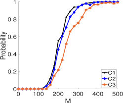
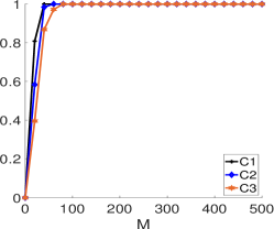
$\underline{\delta}_{10,\mathbf{p}_{\mathrm{opt}}^{(1)}}$



$\underline{\delta}_{10,\mathbf{p}_{\mathrm{opt}}^{(2)}}$



$\underline{\delta}_{10,\mathbf{p}_{\mathrm{opt}}^{(3)}}$







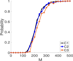
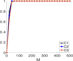
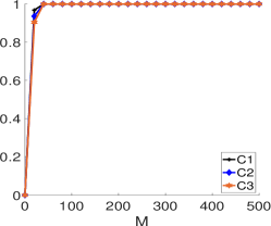
Figure 3:  Probability that $\underline{\delta}_{10}$ is great than $0.005$ as a function of $M$ for $5$ different types of community graphs: $C_{1}$ in black plus, $C_{2}$ in blue diamond, $C_{3}$ in orange hexagon. We choose $M=20:20:500$.





Regime 1



Regime 2



Regime 3







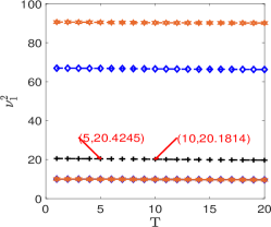
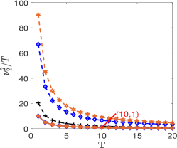
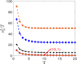
Figure 4:  The relation between spectral graph weighted coherence of order $(k,T)$ and $T$ with $k=10$ and $T$ ranging from 1 to 20 for community graphs.
We present results for $C_{1}$ in black plus, $C_{2}$ in blue diamond, and $C_{3}$ in orange hexagon; uniform sampling distribution in solid curve and optimal sampling distribution in dashed curve.
For regime 1 ,2 and 3, we present the values of $(\nu_{1,\bf{p}^{(1)}}^{k,T})^{2}$, $\sum_{t=0}^{T-1}(\nu_{\bf{p}_{t}^{(2)}})^{2}/T$ and $(\nu_{3,\bf{p}^{(3)}}^{k,T})^{2}/T$, respectively. All figures show that the value are decreasing as $T$ increases, with very slow rate in regime 1 (see two representative data pairs). For the case of optimal sampling distribution, the curves in regime 2 and regime 3 are in fact $10/T$ (see the representative data pair (10,1)). 


We present in Fig. 3 the probabilities that $\underline{\delta}_{10,\mathbf{p}^{(j)}}$ is greater than 0.005, i.e, $\mathrm{Prob}(\underline{\delta}_{10,\mathbf{p}^{(j)}}\geq 0.005)$, estimated over $250$ trials.
Let $M_{i,\mathbf{p}^{(j)}}^{*}$ be the required number of space-time samples to ensure $\mathrm{Prob}(\underline{\delta}_{10,\mathbf{p}^{(j)}}\geq 0.005)=0.9$ for $i$-th graph-type and sampling distribution $\mathbf{p}^{(j)}$ of each sampling regime. Theorem 4.6 predicts that $M_{i,\mathbf{p}^{(j)}}^{*}$ scales linearly with $T(\mathbf{\nu}_{1,\mathbf{p}^{(1)}}^{k,T})^{2}$, $\sum_{t=0}^{T-1}(\mathbf{\nu}_{2,\mathbf{p}^{(2)}}^{k,T}(t))^{2}$ and $(\mathbf{\nu}_{3,\mathbf{p}^{(3)}}^{k,T})^{2}$ for $j=1,2,3$ respectively of community graph $i$.
For the uniform distribution $\mathbf{p}:=\pi$, the first figure from the top panel in Fig. 3 shows that $M_{1,\mathbf{p}^{(j)}}^{*}\geq M_{2,\mathbf{p}^{(j)}}^{*}\geq M_{3,\mathbf{p}^{(j)}}^{*}$. This matches their ordering of $\mathbf{\nu}_{j,\mathbf{p}^{(j)}}^{k,T}$ presented in Fig. 4, and is in accordance with Theorem 4.6. For the optimal sampling distribution $\mathbf{p}_{\mathrm{opt}}$, we have $\mathbf{\nu}_{j,\mathbf{p}_{\textbf{opt}}^{(j)}}^{k,T}$ approximately the same for all types of graphs and $j=1,2,3$. Therefore $M_{i,\mathbf{p}^{(j)}}^{*}$ must be nearly identical for all graph-types, as observed in the second panel of Fig. 3. For each type of graph, in Proposition 9, we showed that for all distributions,




$$\sum_{t=0}^{T-1}(\mathbf{\nu}_{2,\mathbf{p}_{t}^{(2)}}^{k,T})^{2}\leq(\mathbf{\nu}_{3,\mathbf{p}^{(3)}}^{k,T})^{2}\leq T(\mathbf{\nu}_{1,\mathbf{p}^{(1)}}^{k,T})^{2},$$



this matches the numerical results in Fig. 4.


In addition, we also computed the spectral graph weighted coherence for $C_{1}$, $C_{2}$, $C_{3}$ with respect to different sampling distributions and total sampling time $T$ in Fig. 4. The results show that the number of total space-time samples required in regime 2 and regime 3 are the same as $T$ varies and thus one can expect use fewer spatial samples as $T$ increase with approximately 1-1 trade-off. While in regime 1, the temporal information only brings a tiny ratio of reduction in spatial samples.




6.1.2 The results for other graphs


We also perform the same experiments for four other graphs that have wide applications: Minnesota, bunny, path, and sensor graphs (cf. [29]). For the first three graphs, the experiments are performed for bandlimited signals with bandwidth $100$. For the sensor graph, we set the bandwidth $50$. Here our goal is to test the performance with respect to signals with different bandwidth. For the path graph, some eigenvalues have multiplicities larger than 1. We choose the bandwidth to ensure that $\lambda_{k}<\lambda_{k+1}$ as required in our assumptions. The results for $\text{Prob}(\underline{\delta}_{k,\mathbf{p}^{(i)}}>0.005)$ v.s. $M$ are summarized in Fig. 5.





6.2 Comparisons



6.2.1 Optimal distribution versus uniform distribution


Compared with the uniform distribution $\pi^{(j)}$, the optimal distribution $\mathbf{p}_{\textbf{opt}}^{(j)}$ for each regime takes the graph topology and temporal information into account so that one can use fewer space-time samples yet yield robust reconstruction. In the case $k=100$, the advantage of using $\mathbf{p}_{\textbf{opt}}^{(j)}$ is most obvious for the Minnesota and bunny graphs in regime 3. For the Minnesota graph, we reach only a probability of $0.008$ at $M=800$ with $\pi^{(j)}$, whereas $M=400$ are sufficient to reach a probability $1$ with $\mathbf{p}_{\textbf{opt}}^{(j)}$. $\pi^{(j)}$ exhibits a poorer performance for the bunny graph: we reach only a probability of $0.016$ at $M=1400$ with $\pi^{(j)}$, whereas $M=400$ are sufficient to reach a probability 1 with $\mathbf{p}_{\textbf{opt}}^{(j)}$.


Uniform sampling is not working well in regime 3 for the Minnesota and bunny graphs, since there exist few eigenmodes of the bandlimited diffusion field whose energy is highly concentrated on few space-time nodes. In other words, we have $\|\widetilde{U}_{100,T}\delta_{i}\|\approx 1$ for some space-time node $i$. In this case, the corresponding $\nu_{j,\mathbf{\pi}^{(3)}}^{k,T}$ is approximately $\sqrt{Tn}$. In contrast, $\nu_{3,\mathbf{p}_{\textbf{opt}}^{(3)}}^{k,T}$ is $\sqrt{k}$ for $\mathbf{p}_{\textbf{opt}}^{(j)}$. In regime 2, thanks to the the same number of spatial samples taken at consecutive times, the gap between the uniform sampling and optimal sampling is much smaller.


For more regular graphs like the sensor graph and path graph, as our analysis in Section 4.4 shows, the optimal distributions are close to the uniform distributions, and therefore they have comparable performances.


Dynamical sampling versus static sampling. The static sampling ($T=1$) results using uniform distributions are presented in Table 6.2. For path graph and community graph, we observed that the embedding produced by space-time samples chosen according to regime 2 and 3 are as good as the one produced by the same number of spatial samples, we even do better in community graph. For the bunny graph and Minnesota graph, if we count the average spatial samples at each time instance, then we use much fewer spatial samples than the static setting to achieve a comparable performance. From the perspective of sampling, this means that one can use fewer number of sensors and dynamical sampling provides a much cheaper alternative for data acquisition. We also refer to the captions of Figure 6 and Figure 7 for the comparison
of reconstruction with the static case.





Type
Community
Minnesota
Bunny
Path


Regime
1
2
3
1
2
3
1
2
3
1
2
3


$M$
400
80
80
3000
1600
1600
3200
2400
2600
3200
400
400


$M/T$
20
4
4
150
80
80
200
120
120
200
20
20


Static
130
450
$320$
360



Table 6.2: For the uniform distributions, the number of samples that required to reach a probability at least 0.95.




$\text{Minnesota, }\underline{\delta}_{100,\mathbf{p}^{(1)}}$



$\text{Minnesota, }\underline{\delta}_{100,\mathbf{p}^{(2)}}$



$\text{Minnesota, }\underline{\delta}_{100,\mathbf{p}^{(3)}}$







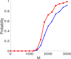
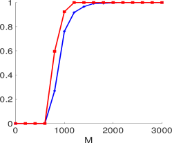
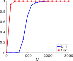
$\text{Bunny, }\underline{\delta}_{100,\mathbf{p}^{(1)}}$



$\text{Bunny, }\underline{\delta}_{100,\mathbf{p}^{(2)}}$



$\text{Bunny, }\underline{\delta}_{100,\mathbf{p}^{(3)}}$







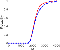
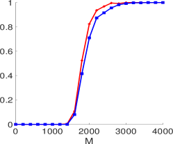
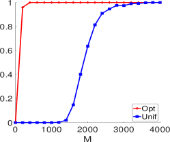
$\text{Sensor, }\underline{\delta}_{50,\mathbf{p}^{(1)}}$



$\text{Sensor, }\underline{\delta}_{50,\mathbf{p}^{(2)}}$



$\text{Sensor, }\underline{\delta}_{50,\mathbf{p}^{(3)}}$







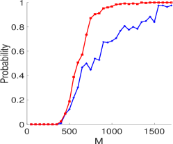
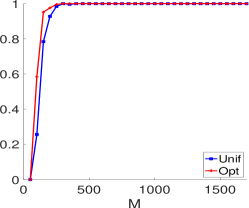
$\text{Path, }\underline{\delta}_{100,\mathbf{p}^{(1)}}$



$\text{Path, }\underline{\delta}_{100,\mathbf{p}^{(2)}}$



$\text{Path, }\underline{\delta}_{100,\mathbf{p}^{(3)}}$







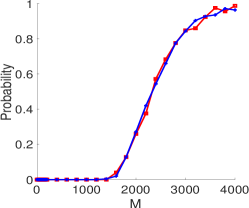
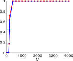
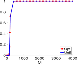
Figure 5:  Probability that $\underline{\delta}_{10}$ is great than $0.005$ as a function of $M$. The panels show the results at $k=100$ for the Minnesota, bunny and path graphs, and at $k=50$ for the sensor graph using optimal and uniform distributions. The gap for $M$ is 200. 


Comparison of sampling regimes. Let $M_{\mathbf{p}^{(j)}}^{*}$ denote the required number of space-time samples in regime $j$ such that $\underline{\delta}_{k,\mathbf{p}^{(j)}}>0.005$. We have found that $M_{\mathbf{p}^{(1)}}^{*}$ is largest for all graphs used in the experiments. And regime 2 has the best performance in terms of the sample complexity. That is to say, we have $M_{\mathbf{p}^{(2)}}^{*}\leq M_{\mathbf{p}^{(3)}}^{*}\leq M_{\mathbf{p}^{(1)}}^{*}$,
which indicates the relationship
$T(\nu_{1,\mathbf{p}^{(1)}}^{K,T})^{2}\geq(\nu_{3,\mathbf{p}^{(3)}}^{K,T})^{2}\geq\sum_{t=0}^{T-1}(\nu_{2,\mathbf{p}^{(2,t)}}^{K,T})^{2}$ for uniform and optimal distributions. These observations coincide with the respective coherence and are consistent with Theorem 4.6 and the analysis in Proposition 4.5.





6.3 Reconstruction of bandlimited signals


In this part, we examine the performance of the reconstruction of initial signals from space-time samples on community graphs of type $C_{3}$, the Minnesota graphs and bunny graphs. We consider the recovery of $k$-bandlimited signals with $k=10$, in contrast with reconstruction results for static sampling setting in [33].
We choose $M=200$ for $\mathbf{p}_{\textbf{opt}}^{(j)}$ with $j=1,2,3$.


The experiments are performed with and without noise on the sampled data. In the presence of noise, the noise vector $\mathbf{e}$ is random with i.i.d. mean 0 and variance $\sigma^{2}$ Gaussian entries .
$\sigma$ are chosen from $\{0,1.5\times 10^{-3},3.7\times 10^{-3},8.8\times 10^{-3},2.1\times 10^{-2},5.0\times 10^{-2}\}$. The signals are reconstructed by solving (22) for different values of the parameter $\gamma$ and different functions $g$. For the community graph and the bunny graph, the regularisation parameter $\gamma$ varies between $10^{-3}$ and $10^{2}$. For the Minnesota graph, it varies between $10^{-1}$ and $10^{5}$. For each $\sigma$, $10$ independent random signals of unit norm are drawn, sampled and reconstructed with all possible $(\gamma,g)$. Then the mean errors $\|x^{*}-x\|_{2}$, $\|{\alpha}^{*}-x\|_{2}$ and $\|{\beta}^{*}\|_{2}$ over these $10$ signals are computed.




Regime 1



Regime 2



Regime3



Community



Community



Community







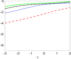
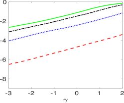
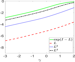
Bunny



Bunny



Bunny







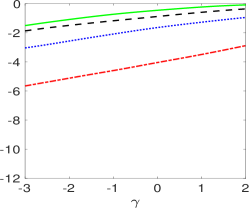
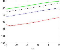
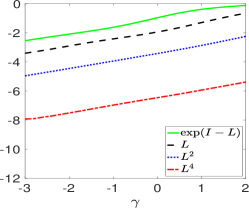
Minesota



Minesota



Minesota







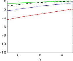
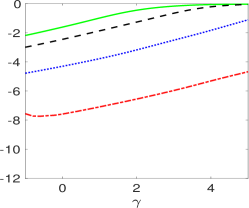
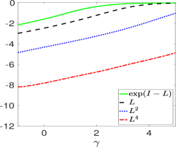
Figure 6: Mean reconstruction errors $\log_{10}\|x-x^{*}\|$ of 10 bandlimited signals as a function of $\gamma$ for the community graph $C_{3}$, Bunny graph and Minnesota graph. We take $M=200$ noise free space-time samples for three regimes. The black dash curve represents results with $g(L)=L$. The blue dotted curves indicate the results with $g(L)=L^{2}$. The red dashed-dot curves indicate the results with $g(L)=L^{4}$. The green solid curve indicate the results with $g(L)=\exp(I-L)$. The first, second and third columns show the results for regime 1, regime 2 and regime 3 using the optimal sampling distribution respectively. We refer to the reconstruction errors of $\|x-\alpha^{*}\|$ and $\|\beta^{*}\|$ in log scale to the supplementary information (SI) section 7.2 (see their definitions in Theorem 5.2). Compared to the static case (Figure 14 in SI), our regime 1 achieved comparable (cf. community graph) or slightly better (cf. bunny and Minesota graphs) performance, and we observed significantly improvement in regime 2 and regime 3.



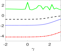
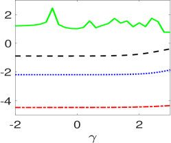
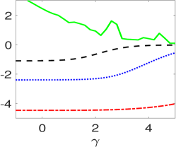
Figure 14: Mean reconstruction error $\log_{10}\|x^{*}-x\|$ in static case $T=1$ from 200 spatial samples. All other parameters are the same with Fig. 6. 

The mean reconstruction errors are presented in Fig. 6 when the measurements are noise-free. In these experiments, the signals are reconstructed by setting $g(L)=L,L^{2},L^{4},\exp(I-L)$. Let’s recall that the ratio $g(\sigma_{k})/g(\sigma_{k+1})$ decreases as the power of $L$ increases. We observe that all reconstruction errors, $\|x^{*}-x\|_{2}$, $\|{\alpha}^{*}-x\|_{2}$ and $\|{{\beta}^{*}}\|_{2}$ decrease when the ratio $g(\sigma_{k})/g(\sigma_{k+1})$ decreases in the range of small $\gamma$ (cf. plots in SI section 7.2), as predicted by the upper bounds in Theorem 5.2. Additionally, Compared to the static case (Figure 14 in SI), our regime 1 achieved comparable (even better) performance, and we observed significantly improvement in regime 2 and 3.


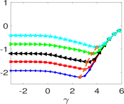
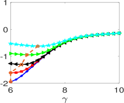
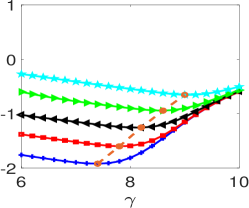
Figure 15: Mean reconstruction error $\log_{10}\|x^{*}-x\|$ in static case $T=1$ from 200 noisy spatial samples. All other parameters are the same with Fig. 7.

We present the mean reconstruction errors when the measurements are noisy in Fig. 7. In these experiments, we reconstruct the signals using $g(L)=L^{4}$. As expected the best regularisation parameter $\gamma$ increases with the noise level. Compared with static sampling setting (cf. Fig 15 in SI section 7.2), our estimates in regime 2 and regime 3 achieve comparable accuracy. The estimates obtained in Regime 1 did not perform as well as other regimes, as indicated by our analysis: one needs to have more space-time samples due to the large spectral graph weighted coherence.




Regime 1



Regime 2



Regime3



Community



Community



Community







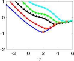
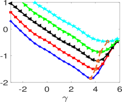
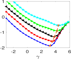
Bunny



Bunny



Bunny







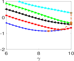
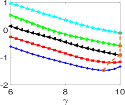
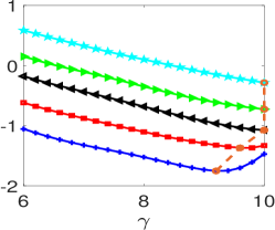
Minesota



Minesota



Minesota







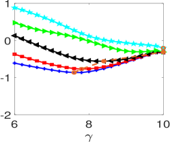
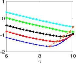
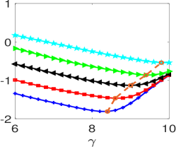
Figure 7: Mean reconstruction error $\log_{10}\|x^{*}-x\|_{2}$ of $10$-bandlimited signals as a function of $\gamma$ with $g(L)=L^{4}$. The simulations are performed in presence of noise. The standard deviation of the noise is $0.0015$ (blue plus), $0.0037$ (red square), $0.0088$ (black left-pointing triangle), $0.0210$ (green right-pointing triangle), $0.0500$ (cyan pentagram). The best reconstruction errors are indicated by orange circles. The first, second and third columns show the results for a community graph of type $C_{5}$, and the Minnesota graph, respectively. The reconstruction accuracy achieved in regime 2 and regime 3 are satisfactory, compared with the static sampling results summarized in Fig. 15 in SI, since we only use 10 spatial samples on average. For bunny graph, we may need to choose bigger $\gamma$, and we expect that the optimal error will also be as comparable with the static case in Fig. 15. 




6.4 Illustration: space-time sampling of a series of blurring real images



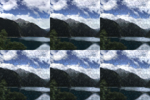
(a) 

Figure 8: The evolved images of the Jiuzhaigou over the first 6 time instances.



The experimental section is finished with an example of de-blurring an image from the space-time samples. We use the photo of Jiuzhaigou park in Sichuan, China. The original photo is (approximately) bandlimited in a nearest neighborhood graph. We consider the heat diffusion process over the graph so we have a series of blurring images. We illustrate the dynamics in Fig. 8.


This RGB image contains $640\times 640$ pixels. We divide this image into patches of $8\times 8$ pixels, thus obtaining $80\times 80$ patches of $64$ pixels per RGB channel. Each patch is denoted by $\mathbf{q}_{i,j,\ell}\in\mathbb{R}^{64}$
with $i\in\{1,\cdots,80\}$, $j\in\{1,\cdots,80\}$, and $\ell\in\{1,2,3\}$. The pair of indices $(i,j)$ encodes the spatial location of the patch and $\ell$ encodes the color channel. Using these patches, we obtain the following matrix




$$X:=\begin{bmatrix}\mathbf{q}_{1,1,1}&\mathbf{q}_{2,1,1}&\cdots&\mathbf{q}_{2,1,1}&\cdots&\mathbf{q}_{80,80,1}\\
\mathbf{q}_{1,1,2}&\mathbf{q}_{2,1,2}&\cdots&\mathbf{q}_{2,1,2}&\cdots&\mathbf{q}_{80,80,2}\\
\mathbf{q}_{1,1,3}&\mathbf{q}_{2,1,3}&\cdots&\mathbf{q}_{2,1,3}&\cdots&\mathbf{q}_{80,80,3}\end{bmatrix}\in\mathbb{R}^{192\times n},n=6400.$$



Each column of $X$ represents a color patch of the original image at a given position.


Motivated by the simulations in [33], we build a graph by modelling the similarity between the columns of $X$. Let $\mathbf{x}_{i}:=X(:,i)\in\mathbb{R}^{192}$. For each $i$, we search for the $20$ nearest
neighbours of $\mathbf{x}_{i}$ among all other columns of $X$. Let $\mathbf{x}_{j}\in\mathbb{R}^{192}$ be a vector connected to $\mathbf{x}_{i}$. The weight $W_{ij}$ of the weighted adjacency matrix $W\in\mathbb{R}^{n\times n}$ satisfies




$$W_{ij}:=\exp\left(-\frac{\|\mathbf{x}_{i}-\mathbf{x}_{j}\|_{2}^{2}}{2\sigma^{2}}\right),$$



where $\sigma>0$ is the standard deviation of all Euclidean distances between pairs of connected columns/patches. We then symmetrize $W$. Each column of $X$ is thus connected to at least $20$ other columns after symmetrization. The construction of the graph is finished by computing the normalized Laplacian $L\in\mathbb{R}^{n\times n}$ associated to $W$. Set the evolution operator $A=\exp(-L)$. We let $A$ act on $X^{\top}$ iteratively with $T=6$ and we treat each column of $X^{\top}$ a bandlimited graph signal with bandwidth 300. For this experiment, we take $M=7200$ measurements using the uniform and optimal distributions for these three sampling regimes and denote the samples as matrix $Y$ which means the samples at each time instance is less than $20\%$ for regime 1 and 2.


The sampled images are presented in Fig. 9, where all non-sampled pixels are in black. The image is reconstructed by solving (22) for each column of Y with $\gamma=10^{-5}$ and $g(L)=L^{4}$. Fig. 10 shows that a very accurate reconstruction of the original image is obtained.
The SNRs between the original and the reconstructed images are presented in Table 6.3. The optimal sampling distribution allows a better image reconstruction quality than the results of the uniform sampling distribution. Additionally, the reconstructions from sampling regimes 2 and 3 have no big difference but both are better than the results from sampling regime 1. The reconstruction results from space-time samples show that incorporating the temporal dynamics is very effective in reducing the spatial sampling density, and one achieved much better performance than the static setting with 4 times higher spatial sampling densities.





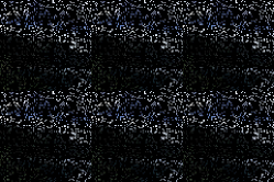
(a) 




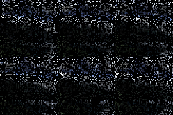
(b) 




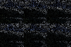
(c) 





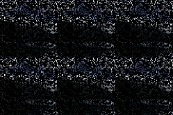
(d) Regime 1




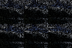
(e) Regime 2




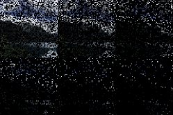
(f) Regime 3



Figure 9: Samples of the real image by using these three sampling regimes:
Top row: uniform sampling. Bottom row: optimal sampling.






(a) 




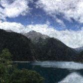
(b) 




(c) 




(d) 




(e) Original





(f) Regime 1




(g) Regime 2




(h) Regime 3



Figure 10: Comparisons of the reconstruction of the real image by using these three sampling regimes with regularizer $\gamma=10^{-5}$:
Top row: Uniform sampling. Bottom row: Optimal sampling.



Table 6.3: The SNR between the original and the reconstructed image: The number of samples per time instance for regime 1,2,3 is 1200 and the total number of samples for static setting is 4800. 




$\gamma=10^{-5}$




Regime 1
Regime 2
Regime 3
Static




Uniform
$22.59$
$27.92$
$28.14$
$21.47$


Optimal
$22.93$
$30.18$
$30.87$
$21.37$








7 Supplementary material



7.1 Proofs



Proof 7.1 (Proof of Proposition 4.5).




 

First let’s prove (a.2).
Notice that




$$\sum_{\ell=1}^{k}\frac{\lambda_{\ell}^{2t}}{f_{T}^{2}(\lambda_{\ell})}=
~{}\sum_{\ell=1}^{k}\sum_{i=1}^{n}(U(i,\ell))^{2}\frac{\lambda_{\ell}^{2t}}{f_{T}^{2}(\lambda_{\ell})}$$





$$=
~{}\sum_{i=1}^{n}\mathbf{p}_{t}^{(2)}(i)\cdot\frac{1}{\mathbf{p}_{t}^{(2)}(i)}\|\widetilde{U}_{k,T}^{\top}\delta_{tn+i}\|_{2}^{2}\leq\left(\nu_{2,\mathbf{p}^{(2)}}^{k,T}(t)\right)^{2}\cdot\sum_{i=1}^{n}\mathbf{p}_{t}^{(2)}(i),$$




the equation holds when $\frac{1}{\mathbf{p}_{t}^{(2)}(i)}\|\widetilde{U}_{k,T}^{\top}\delta_{tn+i}\|_{2}^{2}=\left(\nu_{2,\mathbf{p}^{(2)}}^{k,T}(t)\right)^{2}$ for all $i\in[n]$.
Recall that $\sum_{i=1}^{n}\mathbf{p}_{t}^{(2)}(i)=1$, then we have $\left(\nu_{2,\mathbf{p}^{(2)}}^{k,T}(t)\right)^{2}\geq\sum_{\ell=1}^{k}\frac{\lambda_{\ell}^{2t}}{f_{T}^{2}(\lambda_{\ell})}$. Thus equation holds when $\mathbf{p}_{t}^{(2)}(i)=(\|\widetilde{U}_{k,T}^{\top}\delta_{tn+i}\|_{2}^{2})/(\sum_{\ell=1}^{k}\frac{\lambda_{\ell}^{2t}}{f_{T}^{2}(\lambda_{\ell})})$ for all $i\in[n]$. In particular, we have $\sum_{t=0}^{T-1}\left(\nu_{2,\mathbf{p}^{(2)}}^{k,T}(t)\right)^{2}\geq\sum_{t=0}^{T-1}(\sum_{\ell=1}^{k}\frac{\lambda_{\ell}^{2t}}{f_{T}^{2}(\lambda_{\ell})})=k$.


The proofs for (a.1) and (a.3) are similar to (a.2) by noticing the fact that




$$\sum_{i=1}^{n}\left\|\widetilde{U}_{k,T}((i:n:Tn),:)\right\|_{2}^{2}=
~{}\sum_{i=1}^{n}\mathbf{p}^{(1)}(i)\cdot\frac{1}{\mathbf{p}^{(1)}(i)}\left\|\widetilde{U}_{k,T}((i:n:Tn),:)\right\|_{2}^{2}$$





$$\leq
~{}\sum_{i=1}^{n}\mathbf{p}^{(1)}(i)\cdot\nu_{1,\mathbf{p}^{(1)}}^{k,T}=\nu_{1,\mathbf{p}^{(1)}}^{k,T}$$




and




$$k=\sum_{i=1}^{nT}\|\widetilde{U}_{k,T}^{\top}\delta_{i}\|_{2}^{2}~{}=
~{}\sum_{i=1}^{nT}\mathbf{p}^{(3)}(i)\cdot\frac{1}{\mathbf{p}^{(3)}(i)}\|\widetilde{U}_{k,T}^{\top}\delta_{i}\|_{2}^{2}$$





$$\leq
~{}\sum_{i=1}^{nT}\mathbf{p}^{(3)}(i)\cdot\nu_{3,\mathbf{p}^{(3)}}^{k,T}=\nu_{3,\mathbf{p}^{(3)}}^{k,T}.$$







 

Let’s prove this result when $\mathbf{p}$ is the uniform sampling distribution. The results for the optimal distributions can be derived from part (a) directly.
Let’s first compare $\left(\nu_{1,\mathbf{p}^{(1)}}^{k,T}\right)^{2}$ and $\left(\nu_{3,\mathbf{p}^{(3)}}^{k,T}\right)^{2}$.
Recall the definitions of $\nu_{j,\mathbf{p}^{(j)}}^{k,T}$, $\widetilde{U}_{k,T}$, and $F_{k,T}$, $\Lambda_{k}$ in Definition 4.4, (8), and (2) respectively, we have




$$\left(\nu_{1,\mathbf{p}^{(1)}}^{k,T}\right)^{2}:=
~{}\max_{1\leq i\leq n}\frac{1}{\mathbf{p}^{(1)}(i)}\left\|\widetilde{U}_{k,T}((i:n:Tn),:)\right\|_{2}^{2}$$





$$=
~{}\max_{1\leq i\leq n}n\left\|\sum_{t=0}^{T-1}(F_{k,T}\Lambda_{k}^{t}U_{k}^{\top}\delta_{i}\delta_{i}^{\top}U_{k}\Lambda_{k}^{t}F_{k,T})\right\|_{2}$$





$$\overset{\text{\char 172}}{\geq}
~{}\max_{1\leq i\leq n}\left\{n\cdot\max_{0\leq t\leq T-1}\left\|F_{k,T}\Lambda_{k}^{t}U_{k}^{\top}\delta_{i}\delta_{i}^{\top}U_{k}\Lambda_{k}^{t}F_{k,T}\right\|_{2}\right\}$$





$$=
~{}n\max_{1\leq i\leq n}\max_{0\leq t\leq T-1}\left\|\left[\frac{\lambda_{1}^{t}\cdot U_{k}(i,1)}{f_{T}(\lambda_{1})},\cdots,\frac{\lambda_{k}^{t}\cdot U_{k}(i,k)}{f_{T}(\lambda_{k})}\right]\right\|_{2}^{2}$$





$$=
~{}\frac{1}{T}\left(nT\max_{i,t}\|\widetilde{U}_{k,T}\delta_{tn+i}\|_{2}^{2}\right)=\frac{\left(\nu_{3,\mathbf{p}^{(3)}}^{k,T}\right)^{2}}{T},$$




where ① is coming from that $F_{k,T}\Lambda_{k}^{t}U_{k}^{\top}\delta_{i}\delta_{i}^{\top}U_{k}\Lambda_{k}^{t}F_{k,T}$ is positive semidefinite matrix for all $t$.


Secondly, let’s compare $\nu_{3,\mathbf{p}^{(3)}}^{k,T}$ and $\nu_{2,\mathbf{p}^{(2)}}^{k,T}$. Notice that





(25)

$$\left(\nu_{2,\mathbf{p}^{(2)}}^{k,T}(t)\right)^{2}=
~{}\max_{1\leq i\leq n}\frac{1}{\mathbf{p}_{t}^{(2)}(i)}\|\widetilde{U}_{k,T}^{\top}\delta_{tn+i}\|_{2}^{2}=\max_{1\leq i\leq n}n\|\widetilde{U}_{k,T}^{\top}\delta_{tn+i}\|_{2}^{2}$$





$$\leq
~{}\frac{1}{T}\max_{1\leq j\leq Tn}Tn\|\widetilde{U}_{k,T}^{\top}\delta_{j}\|_{2}^{2}=\frac{1}{T}\left(\nu_{3,\mathbf{p}}^{k,T}\right)^{2}$$





for all $t=0,\cdots,T-1$.
Thus, the conclusions of part (b) are derived.







In order to prove Theorem 4.6, we need the lemma from [42, Theorem 1.1]:



Lemma 7.2.


Let $\{X_{k}\}$ be a finite sequence of independent, random, self-adjoint, positive semi-definite matrices with dimension $d$. Assume that each random matrix satisfies $\lambda_{\max}(X_{k})\leq R$ almost surely.
Define




$$\mu_{\min}:=\lambda_{\min}(\sum_{i}\mathbb{E}(X_{i}))\text{ and }\mu_{\max}:=\lambda_{\max}(\sum_{i}\mathbb{E}(X_{i})).$$



Then




$$\mathbb{P}\left\{\lambda_{\min}(\sum_{i}X_{i})\leq(1-\delta)\mu_{\min}\right\}\leq d\left[\frac{e^{-\delta}}{(1-\delta)^{1-\delta}}\right]^{\mu_{\min}/R},\forall\delta\in[0,1]$$



and




$$\mathbb{P}\left\{\lambda_{\max}(\sum_{i}X_{i})\geq(1+\delta)\mu_{\max}\right\}\leq d\left[\frac{e^{\delta}}{(1+\delta)^{1+\delta}}\right]^{\mu_{\max}/R},\forall\delta\geq 0.$$








Proof 7.3 (Proof of Theorem 4.6).


Let’s first prove the result for regime 2.
$\pi_{A,T}(x)\in\text{span}(\widetilde{U}_{k,T})$, we thus only need to study the property of the matrix $P_{\Omega^{(2)}}^{-1/2}W_{2}^{\frac{1}{2}}S_{2}\widetilde{U}_{k,T}$. Notice that





$$(P_{\Omega^{(2)}}^{-1/2}W_{2}^{\frac{1}{2}}S_{2}\widetilde{U}_{k,T})^{\top}P_{\Omega^{(2)}}^{-1/2}W_{2}^{\frac{1}{2}}S_{2}\widetilde{U}_{k,T}$$




$$=
\sum_{t=0}^{T-1}\sum_{i=1}^{m_{t}}\frac{(F_{k,T}\Lambda_{k}^{t}U_{k}^{\top}\delta_{t,\omega_{t,i}}\delta_{t,\omega_{t,i}}^{\top}U_{k}\Lambda_{k}^{t}F_{k,T})}{m_{t}\mathbf{p}_{t}^{(2)}(\omega_{t,i}^{(2)})}.$$




Set
$X_{t,i}=\frac{F_{k,T}\Lambda_{k}^{t}U_{k}^{\top}\delta_{t,\omega_{t,i}}\delta_{t,\omega_{t,i}}^{\top}U_{k}\Lambda_{k}^{t}F_{k,T}}{m_{t}\mathbf{p}_{t}^{(2)}(\omega_{t,i}^{(2)})}$
and $X:=\sum_{t=0}^{T-1}\sum_{i=1}^{m_{t}}X_{t,i}$.


Thus $X$ is a sum of $M:=\sum_{t=0}^{T-1}m_{t}$ independent, random, self-adjoint, positive semi-definite matrices.
Now let’s estimate $\mu_{\min}$ and $\mu_{\max}$ by computing $\mathbb{E}(X_{t,i})$:




$$\mathbb{E}(X_{t,i})=
\mathbb{E}\left(\frac{F_{k,T}\Lambda_{k}^{t}U_{k}^{\top}\delta_{t,\omega_{t,i}}\delta_{t,\omega_{t,i}}^{\top}U_{k}\Lambda_{k}^{t}F_{k,T}}{m_{t}\mathbf{p}_{t}^{(2)}(\omega_{t,i})}\right)$$





$$=
\sum_{k=1}^{n}\mathbf{p}_{t}^{(2)}(k)\cdot\frac{(F_{k,T}\Lambda_{k}^{t}U_{k}^{\top}\delta_{t,k}\delta_{t,k}^{\top}U_{k}\Lambda_{k}^{t}F_{k,T})}{m_{t}\mathbf{p}_{t}^{(2)}(k)}=\frac{1}{m_{t}}\Lambda_{k}^{2t}F_{k,T}^{2}.$$




Thus $\sum_{t=0}^{T-1}\sum_{i=1}^{m_{t}}\mathbb{E}(X_{t,i})={\mathrm{diag}}(\frac{\sum_{t=0}^{T-1}\lambda_{1}^{2t}}{f_{T}^{2}(\lambda_{1})},\frac{\sum_{t=0}^{T-1}\lambda_{2}^{2t}}{f_{T}^{2}(\lambda_{2})},\cdots,\frac{\sum_{t=0}^{T-1}\lambda_{k}^{2t}}{f_{T}^{2}(\lambda_{k})})=I_{k}$.
Therefore, $\mu_{\min}=\mu_{\max}=1$.
Additionally, for all $X_{t,i}$, we have




$$\begin{aligned} \lambda_{\max}(X_{t,i})=&\left\|X_{t,i}\right\|_{2}=\left\|\frac{F_{k,T}\Lambda_{k}^{t}U_{k}^{\top}\delta_{t,\omega_{t,i}}\delta_{t,\omega_{t,i}}^{\top}U_{k}\Lambda_{k}^{t}F_{k,T}}{m_{t}\mathbf{p}_{t}^{(2)}(\omega_{t,i})}\right\|_{2}\\
\leq&\max_{0\leq t\leq T-1}\max_{1\leq i\leq n}\frac{\|F_{k,T}\Lambda_{k}^{t}U_{k}^{\top}\delta_{t,i}\|_{2}^{2}}{m_{t}\mathbf{p}_{t}^{(2)}(i)}=\max_{0\leq t\leq T-1}\frac{\left(\nu_{2,\mathbf{p}_{t}^{(2)}}^{k,T}(t)\right)^{2}}{m_{t}}=:\nu.\end{aligned}.$$



Lemma 7.1 yields, for any $\delta\in(0,1)$, we have
$\mathbb{P}\left\{\lambda_{\min}(X)\leq 1-\delta\right\}\leq k\left[\frac{e^{-\delta}}{(1-\delta)^{1-\delta}}\right]^{1/\nu}\leq k\exp\left(-\frac{\delta^{2}}{3\nu}\right)$
and $\mathbb{P}\left\{\lambda_{\max}(X)\geq 1+\delta\right\}\leq k\left[\frac{e^{\delta}}{(1+\delta)^{1+\delta}}\right]^{1/\nu}\leq k\exp\left(-\frac{\delta^{2}}{3\nu}\right)$ for all $\delta\in[0,1]$,
here we have used the fact that $\delta+(1-\delta\log(1-\delta))\geq\frac{\delta^{2}}{3}$ and $-\delta+(1+\delta\log(1+\delta))\geq\frac{\delta^{2}}{3}$.
Therefore, for any $\delta\in(0,1)$,



(26)

$$1-\delta\leq\lambda_{\min}(X)\leq\lambda_{\max}(X)\leq 1+\delta$$



holds with probability at least $1-\epsilon$
when $\frac{1}{\nu}\geq\frac{3}{\delta^{2}}\log\left(\frac{2k}{\epsilon}\right)$.
Notice that $m_{t}\geq\frac{3}{\delta^{2}}\left(\nu_{2,\mathbf{p}_{t}^{(2)}}^{k,T}(t)\right)^{2}\log\left(\frac{2k}{\epsilon}\right)$ for all $t=0,\cdots,T-1$ can ensure $\frac{1}{\nu}\geq\frac{3}{\delta^{2}}\log\left(\frac{2k}{\epsilon}\right)$. Thus,




$$(1-\delta)\|\pi_{A,T}(x)\|^{2}\leq\|P_{\Omega^{(2)}}^{-1/2}W_{2}^{\frac{1}{2}}S_{2}\pi_{A,T}(x)\|_{2}^{2}\leq(1+\delta)\|\pi_{A,T}(x)\|_{2}^{2}$$



holds with probability $1-\epsilon$, provided that $m_{t}\geq\frac{3}{\delta^{2}}\left(\nu_{2,\mathbf{p}_{t}^{(2)}}^{k,T}(t)\right)^{2}\log\left(\frac{2k}{\epsilon}\right)$.
Combining Lemma 4.3, we derive the conclusion.


For the results of regime 1 and regime 3, notice that




$$(P_{\Omega^{(1)}}^{-1/2}W_{1}^{\frac{1}{2}}S_{1}\widetilde{U}_{k,T})^{\top}P_{\Omega^{(1)}}^{-1/2}W_{1}^{\frac{1}{2}}S_{1}\widetilde{U}_{k,T}=
\sum_{i=1}^{m}\frac{1}{m\mathbf{p}^{(1)}(i)}\sum_{t=0}^{T-1}F_{k,T}\Lambda_{k}^{t}U_{k}^{\top}\delta_{i}\delta_{i}^{\top}U_{k}\Lambda_{k}^{t}F_{k,T}$$




and




$$(P_{\Omega^{(3)}}^{-1/2}W_{3}^{\frac{1}{2}}S_{3}\widetilde{U}_{k,T})^{\top}P_{\Omega^{(3)}}^{-1/2}W_{3}^{\frac{1}{2}}S_{3}\widetilde{U}_{k,T}=
\sum_{i=1}^{m}\frac{1}{m\mathbf{p}^{(3)}(i)}\widetilde{U}_{k,T}^{\top}\delta_{i}\delta_{i}^{\top}\widetilde{U}_{k,T}$$




Set $X_{i}^{(1)}=\frac{1}{m\mathbf{p}^{(1)}(i)}\sum_{t=0}^{T-1}F_{k,T}\Lambda_{k}^{t}U_{k}^{\top}\delta_{i}\delta_{i}^{\top}U_{k}\Lambda_{k}^{t}F_{k,T}$, $X^{(1)}:=\sum_{i=1}^{m}X_{i}^{(1)}$, $X_{i}^{(3)}=\frac{1}{m\mathbf{p}^{(3)}(i)}\widetilde{U}_{k,T}^{\top}\delta_{i}\delta_{i}^{\top}\widetilde{U}_{k,T}$, and $X^{(3)}:=\sum_{i=1}^{m}X_{i}^{(3)}$. Then $X^{(1)}$ and $X^{(3)}$ are sum of $m$ independent, random, self-adjoint, positive semi-definite matrices. Similar to the proof for regime 2, we can get the results for regime 1 and 3.





Proof 7.4 (Proof of Theorem 5.1).


Note that ${\mathbf{x}}^{*}$ is a solution to (17). Thus by optimality of ${\mathbf{x}}^{*}$, we obtain



(27)

$$\|P_{\Omega^{(j)}}^{-1/2}W_{j}^{\frac{1}{2}}(S_{j}\pi_{A,T}({\mathbf{x}}^{*})-\mathbf{y})\|_{2}\leq\|P_{\Omega^{(j)}}^{-1/2}W_{j}^{\frac{1}{2}}(S_{j}\pi_{A,T}(\widetilde{\mathbf{x}})-\mathbf{y})\|$$



for any $\widetilde{\mathbf{x}}\in\text{span}(U_{k})$. In particular, for $\widetilde{\mathbf{x}}=\mathbf{x}$, we have



(28)

$$\small\|P_{\Omega^{(j)}}^{-1/2}W_{j}^{\frac{1}{2}}S_{j}\pi_{A,T}({\mathbf{x}}^{*})-\mathbf{y})\|_{2}\leq\|P_{\Omega^{(j)}}^{-1/2}W_{j}^{\frac{1}{2}}(S_{j}\pi_{A,T}(\mathbf{x})-\mathbf{y})\|=\|P_{\Omega^{(j)}}^{-1/2}W_{j}^{\frac{1}{2}}\mathbf{e}\|.$$



Notice that



(29)


$$\|P_{\Omega^{(j)}}^{-1/2}W_{j}^{\frac{1}{2}}S_{j}\pi_{A,T}({\mathbf{x}}^{*})-\mathbf{y})\|_{2}$$




$$=
\|P_{\Omega^{(j)}}^{-1/2}W_{j}^{\frac{1}{2}}S_{j}\pi_{A,T}({\mathbf{x}}^{*})-P_{\Omega^{(j)}}^{-1/2}W_{j}^{\frac{1}{2}}S_{j}\pi_{A,T}(\mathbf{x})-P_{\Omega^{(j)}}^{-1/2}W_{j}^{\frac{1}{2}}\mathbf{e}\|_{2}$$





$$\geq
\|P_{\Omega^{(j)}}^{-1/2}W_{j}^{\frac{1}{2}}S_{j}\pi_{A,T}({\mathbf{x}}^{*}-\mathbf{x})\|_{2}-\|P_{\Omega^{(j)}}^{-1/2}W_{j}^{\frac{1}{2}}\mathbf{e}\|_{2}$$





$$\geq
\sqrt{1-\delta}f_{T}(\lambda_{k})\|{\mathbf{x}}-\mathbf{x}^{*}\|_{2}-\|P_{\Omega^{(j)}}^{-1/2}W_{j}^{\frac{1}{2}}\mathbf{e}\|_{2}.$$





Combing (27)–(29), the following inequality holds




$$\|P_{\Omega^{(j)}}^{-1/2}W_{j}^{\frac{1}{2}}\mathbf{e}\|\geq\sqrt{1-\delta}f_{T}(\lambda_{k})\|{\mathbf{x}}-\mathbf{x}^{*}\|_{2}-\|P_{\Omega^{(j)}}^{-1/2}W_{j}^{\frac{1}{2}}\mathbf{e}\|_{2}.$$



Thus, we have the first bound




$$\|\mathbf{x}^{*}-{\mathbf{x}}\|_{2}\leq\frac{2}{\sqrt{1-\delta}f_{T}(\lambda_{k})}\|P_{\Omega^{(j)}}^{-1/2}W_{j}^{\frac{1}{2}}\mathbf{e}\|_{2}.$$





To prove the second bound, let us choose $\mathbf{e}_{0}=S_{j}\pi_{A,T}(\mathbf{x}_{0})$ for some $\mathbf{x}_{0}\in\text{span}(U_{k})$. Therefore, $\mathbf{y}=S_{j}(\pi_{A,T}(\mathbf{x}_{0}+\mathbf{x}))$ and ${\mathbf{x}}^{*}=\mathbf{x}+\mathbf{x}_{0}$ is a solution for (17) in this case. By Theorem 4.6, we have




$$\|{\mathbf{x}}-\mathbf{x}^{*}\|_{2}=\|\mathbf{x}_{0}\|_{2}\geq
\frac{1}{\sqrt{1+\delta}f_{T}(\lambda_{1})}\|P_{\Omega^{(j)}}^{-1/2}W_{j}S_{j}\pi_{A,T}(\mathbf{x}_{0})\|_{2}$$





$$=
\frac{1}{\sqrt{1+\delta}f_{T}(\lambda_{1})}\|P_{\Omega^{(j)}}^{-1/2}W_{j}^{\frac{1}{2}}S_{j}\pi_{A,T}(\mathbf{x}_{0})\|_{2}$$





$$=
\frac{1}{\sqrt{1+\delta}f_{T}(\lambda_{1})}\|P_{\Omega^{(j)}}^{-1/2}W_{j}^{\frac{1}{2}}\mathbf{e}_{0}\|_{2}.$$




The proof of Theorem 5.1 is completed.





Proof 7.5 (Proof of Theorem 5.2 ).


Since ${\mathbf{x}}^{*}$ is a solution to (22), we have for all $\widetilde{\mathbf{x}}\in\mathbb{R}^{n}$



(30)

$$\begin{aligned} &\|P_{\Omega^{(j)}}^{-1/2}W_{j}^{\frac{1}{2}}(S_{j}\pi_{A,T}(\mathbf{x}^{*})-\mathbf{y})\|_{2}^{2}+\gamma(\mathbf{x}^{*})^{T}g(L)\mathbf{x}^{*}\\
\leq&\|P_{\Omega^{(j)}}^{-1/2}W_{j}^{\frac{1}{2}}(S_{j}\pi_{A,T}(\widetilde{\mathbf{x}})-\mathbf{y})\|_{2}^{2}+\gamma\widetilde{\mathbf{x}}^{\top}g(L)\widetilde{\mathbf{x}}\end{aligned}.$$



We also have $\mathbf{x}^{*}=\mathbf{\alpha}^{*}+\mathbf{\beta}^{*}$ with $\mathbf{\alpha}^{*}\in\text{span}(U_{k})$ and $\mathbf{\beta}^{*}\in\text{span}(U_{k})^{\perp}=\text{span}(\overline{U}_{k})$, where the matrix $\overline{U}_{k}$ is defined as
$\overline{U}_{k}:=(\mathbf{u}_{k+1},\cdots,\mathbf{u}_{n})\in\mathbb{R}^{n\times(n-k)}$.


Choosing $\widetilde{\mathbf{x}}=\mathbf{x}$ in (30) and using the fact that $U_{k}^{\top}\beta^{*}=0$, $\overline{U}_{k}^{\top}\alpha^{*}=0$, $\overline{U}_{k}^{\top}\mathbf{x}=0$, and the eigen-decomposition of $g(L)$ is $g(L)=Ug(\Sigma)U^{\top}$, we obtain that



(31)


$$\|P_{\Omega^{(j)}}^{-1/2}W_{j}^{\frac{1}{2}}(S_{j}\pi_{A,T}(\mathbf{x}^{*})-\mathbf{y})\|_{2}^{2}+\gamma(\mathbf{x}^{*})^{T}g(L)\mathbf{x}^{*}$$




$$=
\|P_{\Omega^{(j)}}^{-1/2}W_{j}^{\frac{1}{2}}(S_{j}\pi_{A,T}(\mathbf{x}^{*})-\mathbf{y})\|_{2}^{2}+\gamma(U_{k}^{\top}\alpha^{*})^{T}g(\Sigma_{k})(U_{k}^{\top}\alpha^{*})$$






$$~{}+\gamma(\overline{U}_{k}^{\top}\beta^{*})^{T}g(\overline{\Sigma}_{k})(\overline{U}_{k}^{\top}\beta^{*})$$




$$\leq
\|P_{\Omega^{(j)}}^{-1/2}W_{j}^{\frac{1}{2}}(S_{j}\pi_{A,T}(\mathbf{x})-\mathbf{y})\|_{2}^{2}+\gamma\mathbf{x}^{T}g(L)\mathbf{x}$$





$$=
\|P_{\Omega^{(j)}}^{-1/2}W_{j}^{\frac{1}{2}}\mathbf{e}\|_{2}^{2}+\gamma(U_{k}^{\top}\mathbf{x})^{T}g(\Sigma_{k})(U_{k}^{\top}\mathbf{x}),$$





where
$g(\Sigma_{k})={\mathrm{diag}}(g(\sigma_{1}),\cdots,g(\sigma_{k}))$ and $g(\overline{\Sigma}_{k})={\mathrm{diag}}(g(\sigma_{k+1}),\cdots,g(\sigma_{n}))$.


Notice that




$$(U_{k}^{\top}\alpha^{*})^{T}g(\Sigma_{k})(U_{k}^{\top}\alpha^{*})\geq 0,$$







$$(\overline{U}_{k}^{\top}\beta^{*})^{T}g(\overline{\Sigma}_{k})(\overline{U}_{k}^{\top}\beta^{*})\geq g(\sigma_{k+1})\|\overline{U}_{k}^{\top}\beta^{*}\|_{2}^{2}=g(\sigma_{k+1})\|\beta^{*}\|_{2}^{2}$$



and




$$(U_{k}^{\top}\mathbf{x})^{T}g(\Sigma_{k})(U_{k}^{\top}\mathbf{x})\leq g(\sigma_{k})\|U_{k}^{\top}\mathbf{x}\|_{2}^{2}=g(\sigma_{k})\|\mathbf{x}\|_{2}^{2}.$$



Combining (31), we thus have



(32)

$$\small\|P_{\Omega^{(j)}}^{-1/2}W_{j}^{\frac{1}{2}}S_{j}\pi_{A,T}(\mathbf{x}^{*})-\mathbf{y})\|_{2}^{2}+\gamma g(\sigma_{k+1})\|\beta^{*}\|_{2}^{2}\leq\|P_{\Omega^{(j)}}^{-1/2}W_{j}^{\frac{1}{2}}\mathbf{e}\|_{2}^{2}+\gamma g(\sigma_{k})\|\mathbf{x}\|_{2}^{2}.$$



As the left hand side of (32) is a sum of two positive quantities, we also have



(33)


$$\|P_{\Omega^{(j)}}^{-1/2}W_{j}^{\frac{1}{2}}(S_{j}\pi_{A,T}(\mathbf{x}^{*})-\mathbf{y})\|_{2}^{2}$$




$$\leq
\|P_{\Omega^{(j)}}^{-1/2}W_{j}^{\frac{1}{2}}\mathbf{e}\|_{2}^{2}+\gamma g(\sigma_{k})\|\mathbf{x}\|_{2}^{2}\leq(\|P_{\Omega^{(j)}}^{-1/2}W_{j}^{\frac{1}{2}}\mathbf{e}\|_{2}+\sqrt{\gamma g(\sigma_{k})}\|\mathbf{x}\|_{2})^{2}$$





and



(34)

$$\gamma g(\sigma_{k+1})\|\beta^{*}\|_{2}^{2}\leq(\|P_{\Omega^{(j)}}^{-1/2}W_{j}^{\frac{1}{2}}\mathbf{e}\|_{2}+\sqrt{\gamma g(\sigma_{k})}\|\mathbf{x}\|_{2})^{2}.$$



Thus, we have
$\|P_{\Omega^{(j)}}^{-1/2}W_{j}^{\frac{1}{2}}S_{j}\pi_{A,T}(\mathbf{x}^{*})-\mathbf{y})\|_{2}\leq\|P_{\Omega^{(j)}}^{-1/2}W_{j}^{\frac{1}{2}}\mathbf{e}\|_{2}+\sqrt{\gamma g(\sigma_{k})}\|\mathbf{x}\|_{2}$ and
$\sqrt{\gamma g(\sigma_{k+1})}\|\beta^{*}\|_{2}\leq\|P_{\Omega^{(j)}}^{-1/2}W_{j}^{\frac{1}{2}}\mathbf{e}\|_{2}+\sqrt{\gamma g(\sigma_{k})}\|\mathbf{x}\|_{2}$.
The second inequality yields (24).
It remains to prove (23). Recall that





$$\|P_{\Omega^{(j)}}^{-1/2}W_{j}^{\frac{1}{2}}(S_{j}\pi_{A,T}(\mathbf{x}^{*})-\mathbf{y})\|_{2}$$




$$=
\|P_{\Omega^{(j)}}^{-1/2}W_{j}^{\frac{1}{2}}(S_{j}\pi_{A,T}(\alpha^{*}-\mathbf{x}))-P_{\Omega^{(j)}}^{-1/2}W_{j}^{\frac{1}{2}}(S_{j}\pi_{A,T}(\beta^{*})+\mathbf{e})\|_{2}$$





$$\geq
\|P_{\Omega^{(j)}}^{-1/2}W_{j}^{\frac{1}{2}}(S_{j}\pi_{A,T}(\alpha^{*}-\mathbf{x}))\|_{2}-\|P_{\Omega^{(j)}}^{-1/2}W_{j}^{\frac{1}{2}}\mathbf{e}\|_{2}-\|P_{\Omega^{(j)}}^{-1/2}W_{j}^{\frac{1}{2}}S_{j}\pi_{A,T}(\beta^{*})\|_{2}$$





$$\geq
\sqrt{1-\delta}f_{T}(\lambda_{k})\|\alpha^{*}-\mathbf{x}\|_{2}-\|P_{\Omega^{(j)}}^{-1/2}W_{j}^{\frac{1}{2}}\mathbf{e}\|_{2}-M_{\max}\|\pi_{A,T}(\beta^{*})\|_{2}.$$




Since $\beta^{*}\in\text{span}(\overline{U}_{k})$, we have $\|\pi_{A,T}(\beta^{*})\|_{2}\leq f_{T}(\lambda_{k+1})\|\beta^{*}\|_{2}$. Therefore,



(35)


$$\|P_{\Omega^{(j)}}^{-1/2}W_{j}^{\frac{1}{2}}(S_{j}\pi_{A,T}(\mathbf{x}^{*})-\mathbf{y})\|_{2}$$




$$\geq
\sqrt{1-\delta}f_{T}(\lambda_{k})\|\alpha^{*}-\mathbf{x}\|_{2}-\|P_{\Omega^{(j)}}^{-1/2}W_{j}^{\frac{1}{2}}\mathbf{e}\|_{2}-M_{\max}f_{T}(\lambda_{k+1})\|\beta^{*}\|_{2}.$$





Combing (33) and (35), we have





$$\|P_{j}^{-1/2}W_{j}^{\frac{1}{2}}\mathbf{e}\|_{2}+\sqrt{\gamma g(\sigma_{k})}\|\mathbf{x}\|_{2}$$




$$\geq
\sqrt{1-\delta}f_{T}(\lambda_{k})\|\alpha^{*}-\mathbf{x}\|_{2}-\|P_{j}^{-1/2}W_{j}^{\frac{1}{2}}\mathbf{e}\|_{2}-M_{\max}f_{T}(\lambda_{k+1})\|\beta^{*}\|_{2}$$





$$\geq
\sqrt{1-\delta}f_{T}(\lambda_{k})\|\alpha^{*}-\mathbf{x}\|_{2}-\|P_{j}^{-1/2}W_{j}^{\frac{1}{2}}\mathbf{e}\|_{2}-$$






$$M_{\max}f_{T}(\lambda_{k+1})\left(\frac{1}{\sqrt{\gamma g(\sigma_{k+1})}}\|P_{\Omega^{(j)}}^{-1/2}W_{j}\mathbf{e}\|_{2}+\left(\sqrt{\frac{g(\sigma_{k})}{g(\sigma_{k+1})}}\|\mathbf{x}\|_{2}\right)\right).$$



Thus the conclusion (23)
holds.






7.2 Additional numerical results


In this section, we present results for the reconstruction errors $\|x-\alpha^{*}\|_{2}$ and $\|\beta^{*}\|$ for all graphs, in the spirit of Theorem 5.2, see Fig. 12 and 13, complementary to Fig. 6.


We present mean reconstruction errors of 10 bandlimited signals as a function of $\gamma$. We take $M=200$ noise free space-time samples for three regimes. The back curve represents results with $g({L})={L}$. The blue curves indicate the results with $g({L})={L}^{2}$. The red curves indicate the results with $g({L})={L}^{4}$. The green curve indicates the results with $g({L})=\exp(I-L)$. The first, second and third columns show the results for regime 1, regime 2 and regime 3 using the optimal sampling distribution respectively. The first and second rows show the mean reconstruction errors $\|x-\alpha^{*}\|$ and $\|\beta^{*}\|$ respectively.


Comparison to the static case


We also plot the reconstruction results by changing $T=1$.




Regime 1



Regime 2



Regime3











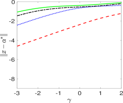
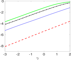
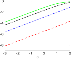
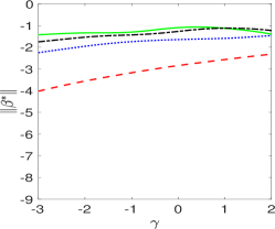
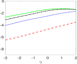
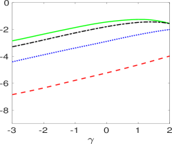
Figure 11: Community graph $C_{5}$ 




Regime 1



Regime 2



Regime3











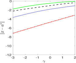
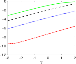
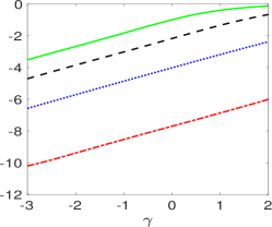
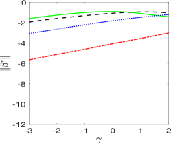
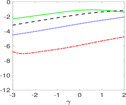
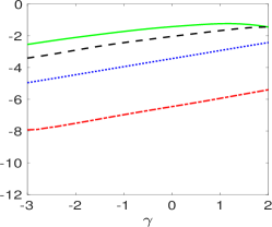
Figure 12:  Bunny graph. 




Regime 1



Regime 2



Regime3











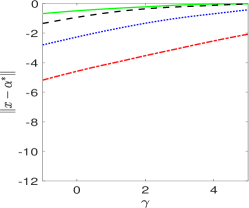
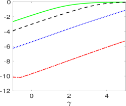
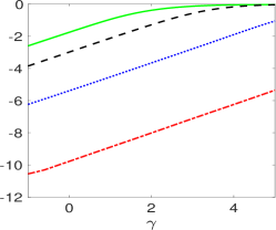
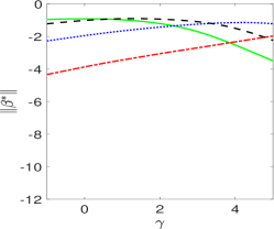
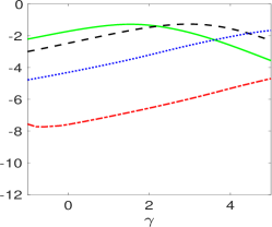
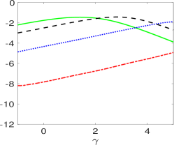
Figure 13: Minnesota graph 




Community



Bunny



Minesota










Community



Bunny



Minesota

References

[1]R. Aceska, A. Aldroubi, J. Davis, and A. Petrosyan, Dynamical
sampling in shift invariant spaces, Commutative and Noncommutative Harmonic
Analysis and Applications, 603 (2013), pp. 139–148.
[2]A. Aldroubi, C. Cabrelli, U. Molter, and S. Tang, Dynamical
sampling, Applied and Computational Harmonic Analysis, 42 (2017),
pp. 378–401.
[3]A. Aldroubi, J. Davis, and I. Krishtal, Dynamical sampling:
Time–space trade-off, Applied and Computational Harmonic Analysis, 34
(2013), pp. 495–503.
[4]A. Aldroubi, K. Gröchenig, L. Huang, P. Jaming, I. Krishtal, and J. L.
Romero, Sampling the flow of a bandlimited function, The Journal of
Geometric Analysis, (2021), pp. 1–35.
[5]A. Aldroubi, L. Huang, and A. Petrosyan, Frames induced by the
action of continuous powers of an operator, Journal of Mathematical Analysis
and Applications, 478 (2019), pp. 1059–1084.
[6]A. Aldroubi, I. Krishtal, and S. Tang, Phaseless reconstruction from
space–time samples, Applied and Computational Harmonic Analysis, 48 (2020),
pp. 395–414.
[7]A. Anis, A. Gadde, and A. Ortega, Efficient sampling set selection
for bandlimited graph signals using graph spectral proxies, IEEE
Transactions on Signal Processing, 64 (2016), pp. 3775–3789.
[8]C. Cabrelli, U. Molter, V. Paternostro, and F. Philipp, Dynamical
sampling on finite index sets, Journal d’Analyse Mathématique, 140
(2020), pp. 637–667.
[9]M. Ceccon, Graph signal processing: Reconstruction algorithms,
(2017).
[10]L. F. Chamon and A. Ribeiro, Greedy sampling of graph signals, IEEE
Transactions on Signal Processing, 66 (2017), pp. 34–47.
[11]S. Chen, F. Cerda, P. Rizzo, J. Bielak, J. H. Garrett, and
J. Kovačević, Semi-supervised multiresolution classification
using adaptive graph filtering with application to indirect bridge structural
health monitoring, IEEE Transactions on Signal Processing, 62 (2014),
pp. 2879–2893.
[12]S. Chen, A. Sandryhaila, J. M. Moura, and J. Kovačević, Adaptive graph filtering: Multiresolution classification on graphs, in 2013
IEEE Global Conference on Signal and Information Processing, IEEE, 2013,
pp. 427–430.
[13]S. Chen, R. Varma, A. Sandryhaila, and J. Kovačević, Discrete signal processing on graphs: Sampling theory, IEEE Transactions on
Signal Processing, 63 (2015), pp. 6510–6523.
[14]S. Chen, R. Varma, A. Singh, and J. Kovacević, Signal recovery
on graphs: Random versus experimentally designed sampling, in 2015
International Conference on Sampling Theory and Applications (SampTA), IEEE,
2015, pp. 337–341.
[15]S. Chen, R. Varma, A. Singh, and J. Kovačević, Signal
recovery on graphs: Fundamental limits of sampling strategies, IEEE
Transactions on Signal and Information Processing over Networks, 2 (2016),
pp. 539–554.
[16]O. Christensen and M. Hasannasab, Frame properties of systems
arising via iterated actions of operators, Applied and Computational
Harmonic Analysis, 46 (2019), pp. 664–673.
[17]G. Davis, S. Mallat, and M. Avellaneda, Adaptive greedy
approximations, Constructive Approximation, 13 (1997), pp. 57–98.
[18]I. Dokmanić, J. Ranieri, A. Chebira, and M. Vetterli, Sensor
networks for diffusion fields: Detection of sources in space and time, in
2011 49th Annual Allerton Conference on Communication, Control, and Computing
(Allerton), IEEE, 2011, pp. 1552–1558.
[19]V. N. Ekambaram, G. Fanti, B. Ayazifar, and K. Ramchandran, Wavelet-regularized graph semi-supervised learning, in 2013 IEEE Global
Conference on Signal and Information Processing, IEEE, 2013, pp. 423–426.
[20]A. Hashemi, R. Shafipour, H. Vikalo, and G. Mateos, Accelerated
sampling of bandlimited graph signals, arXiv preprint arXiv:1807.07222,
(2018).
[21]C. Huang, Q. Zhang, J. Huang, and L. Yang, Reconstruction of
bandlimited graph signals from measurements, Digital Signal Processing, 101
(2020), p. 102728.
[22]E. Isufi, P. Banelli, P. Di Lorenzo, and G. Leus, Observing and
tracking bandlimited graph processes from sampled measurements, Signal
Processing, 177 (2020), p. 107749.
[23]C.-K. LAI and S. TANG, Undersampled windowed exponentials, spectra
of toeplitz operators and its applications, arXiv preprint arXiv:1702.01887,
(2017).
[24]A. Loukas and D. Foucard, Frequency analysis of time-varying graph
signals, in 2016 IEEE Global Conference on Signal and Information Processing
(GlobalSIP), IEEE, 2016, pp. 346–350.
[25]Y. M. Lu and M. Vetterli, Spatial super-resolution of a diffusion
field by temporal oversampling in sensor networks, in 2009 IEEE
International Conference on Acoustics, Speech and Signal Processing, IEEE,
2009, pp. 2249–2252.
[26]A. G. Marques, S. Segarra, G. Leus, and A. Ribeiro, Sampling of
graph signals with successive local aggregations, IEEE Transactions on
Signal Processing, 64 (2015), pp. 1832–1843.
[27]J. Murray-Bruce and P. L. Dragotti, Estimating localized sources of
diffusion fields using spatiotemporal sensor measurements, IEEE Transactions
on Signal Processing, 63 (2015), pp. 3018–3031.
[28]J. Murray-Bruce and P. L. Dragotti, Physics-driven quantized
consensus for distributed diffusion source estimation using sensor networks,
EURASIP Journal on Advances in Signal Processing, 2016 (2016), pp. 1–22.
[29]N. Perraudin, J. Paratte, D. Shuman, L. Martin, V. Kalofolias,
P. Vandergheynst, and D. K. Hammond, Gspbox: A toolbox for signal
processing on graphs, arXiv preprint arXiv:1408.5781, (2014).
[30]I. Pesenson, Sampling in paley-wiener spaces on combinatorial
graphs, Transactions of the American Mathematical Society, 360 (2008),
pp. 5603–5627.
[31]I. Pesenson, Variational splines and paley–wiener spaces on
combinatorial graphs, Constructive Approximation, 29 (2009), pp. 1–21.
[32]I. Z. Pesenson and M. Z. Pesenson, Sampling, filtering and sparse
approximations on combinatorial graphs, Journal of Fourier Analysis and
Applications, 16 (2010), pp. 921–942.
[33]G. Puy, N. Tremblay, R. Gribonval, and P. Vandergheynst, Random
sampling of bandlimited signals on graphs, Applied and Computational
Harmonic Analysis, 44 (2018), pp. 446–475.
[34]K. Qiu, X. Mao, X. Shen, X. Wang, T. Li, and Y. Gu, Time-varying
graph signal reconstruction, IEEE Journal of Selected Topics in Signal
Processing, 11 (2017), pp. 870–883.
[35]J. Ranieri, A. Chebira, Y. M. Lu, and M. Vetterli, Sampling and
reconstructing diffusion fields with localized sources, in 2011 IEEE
International Conference on Acoustics, Speech and Signal Processing (ICASSP),
IEEE, 2011, pp. 4016–4019.
[36]A. Sandryhaila and J. M. Moura, Big data analysis with signal
processing on graphs: Representation and processing of massive data sets with
irregular structure, IEEE Signal Processing Magazine, 31 (2014), pp. 80–90.
[37]S. Segarra, A. G. Marques, G. Leus, and A. Ribeiro, Reconstruction
of graph signals through percolation from seeding nodes, IEEE Transactions
on Signal Processing, 64 (2016), pp. 4363–4378.
[38]D. I. Shuman, S. K. Narang, P. Frossard, A. Ortega, and P. Vandergheynst,
The emerging field of signal processing on graphs: Extending
high-dimensional data analysis to networks and other irregular domains, IEEE
Signal Processing Magazine, 30 (2013), pp. 83–98.
[39]O. Sporns, Networks of the Brain, MIT press, 2010.
[40]S. Tang, Universal spatiotemporal sampling sets for discrete
spatially invariant evolution processes, IEEE Transactions on Information
Theory, 63 (2017), pp. 5518–5528.
[41]D. Thanou, X. Dong, D. Kressner, and P. Frossard, Learning heat
diffusion graphs, IEEE Transactions on Signal and Information Processing
over Networks, 3 (2017), pp. 484–499.
[42]J. A. Tropp, User-friendly tail bounds for sums of random matrices,
Foundations of Computational Mathematics, 12 (2012), pp. 389–434.
[43]A. Ulanovskii and I. Zlotnikov, Reconstruction of bandlimited
functions from space–time samples, Journal of Functional Analysis, 280
(2021), p. 108962.
[44]D. Valsesia, G. Fracastoro, and E. Magli, Sampling of graph signals
via randomized local aggregations, IEEE Transactions on Signal and
Information Processing over Networks, 5 (2018), pp. 348–359.
[45]X. Wang, J. Chen, and Y. Gu, Local measurement and reconstruction
for noisy bandlimited graph signals, Signal Processing, 129 (2016),
pp. 119–129.
[46]X. Wang, M. Wang, and Y. Gu, A distributed tracking algorithm for
reconstruction of graph signals, IEEE Journal of Selected Topics in Signal
Processing, 9 (2015), pp. 728–740.
[47]Y. Xiao, D. Chen, S. Wei, Q. Li, H. Wang, and M. Xu, Rumor
propagation dynamic model based on evolutionary game and anti-rumor,
Nonlinear Dynamics, 95 (2019), pp. 523–539.
[48]G. Yang, L. Yang, and C. Huang, An orthogonal partition selection
strategy for the sampling of graph signals with successive local
aggregations, Signal Processing, (2021), p. 108211.
[49]H. Yu, Z. Wu, S. Wang, Y. Wang, and X. Ma, Spatiotemporal recurrent
convolutional networks for traffic prediction in transportation networks,
Sensors, 17 (2017), p. 1501.