Solution decomposition for the nonlinear Poisson-Boltzmann equation using the range-separated tensor format

Abstract

The Poisson-Boltzmann equation (PBE) is an implicit solvent continuum model for calculating the electrostatic potential and energies of charged biomolecules in ionic solutions. However, its numerical solution poses a significant challenge due strong singularities and nonlinearity caused by the singular source terms and the exponential nonlinear terms, respectively. An efficient method for the treatment of singularities in the linear PBE which was introduced in [1], that is based on the range-separated (RS) tensor decomposition [2] for both electrostatic potential and the discretized Dirac delta distribution [3]. In this paper, we extend this regularization method to the nonlinear PBE. Similar to [1] we apply the PBE only to the regular part of the solution corresponding to the modified right-hand side via extraction of the long-range part in the discretized Dirac delta distribution. The total electrostatic potential is obtained by adding the long-range solution to the directly precomputed short-range potential. The main computational benefit of the approach is the automatic preservation of the continuity in the Cauchy data on the solute-solvent interface. The boundary conditions are also obtained from the long-range component of the precomputed canonical tensor representation of the Newton kernel. In the numerical experiments, we illustrate the accuracy of the nonlinear regularized PBE (NRPBE) over the classical variant.

Key words: Poisson-Boltzmann equation, electrostatic potential, singular source terms, Newton kernel, long- and short-range solution, low-rank tensor decompositions, range-separated tensor formats.

AMS Subject Classification: 65F30, 65F50, 65N35, 65F10

1 Introduction

Biochemical processes are occurring between macromolecules such as proteins and nucleic acids in solution at a physiological salt concentration. The resultant electrostatic interactions are highly relevant for an understanding of biological functions and structures of biomolecules, enzyme catalysis, molecular recognition, and biomolecular encounter or association rates [4, 5, 6, 7]. Efficient modeling of these interactions remains a great challenge in computational biology because of the complexity of biomolecular systems which are dominated by the effects of solvation on biomolecular processes and by the long-range intermolecular interactions [8, 9, 10].

There are two main types of models which can be used to model electrostatic interactions in ionic solutions. The explicit approaches which treat both the solute and solvent in atomic detail, are generally computationally demanding. This is because they require substantial sampling and equilibration in order to converge the properties of interest in an ensemble of solute and solvent [10, 11]. On the other hand, continuum or implicit approaches treat the solvent molecules as a continuum, by integrating out non-relevant degrees of freedom in order to circumvent the need for sampling and equilibration [12, 10, 11].

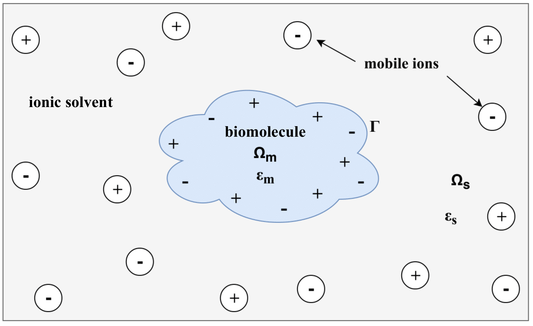
Figure 1.1: Representation of a biomolecule with partial charges and an internal dielectric constant ${\epsilon}_{m}$ in a solvent with dielectric constant ${\epsilon}_{s}$ of mobile ions. Figure courtesy [13].

There exists a number of implicit solvation approaches for biomolecules [12, 14, 10], but the most popular is based on the Poisson-Boltzmann equation (PBE), which was extensively analyzed, for example, in [15]. The PBE is used for calculating the electrostatic potential and energies of charged or partially charged biomolecules in a physiological environment. We present the PBE model in Section 2.

It is impossible to obtain analytic solutions of the PBE for biomolecules with complex geometries and highly singular charge distributions [15, 16]. The numerical solution of the PBE was pioneered by Warwicker and Watson in 1982 [17], where the electrostatic potential was computed at the active site of an enzyme using the finite difference method (FDM). Besides the FDM [18, 19], other numerical techniques such as the finite element methods (FEM) [18, 20] and the boundary element methods (BEM) [21, 22] have hitherto successfully been used to solve the PBE, see [23] for a thorough review. However, the numerical solution of the PBE is faced with a number of challenges. The most significant are the strong charge singularities caused by the singular source terms (Dirac delta distribution), the nonlinearity caused by the exponential nonlinear terms, the unbounded domain due to slow polynomial decay of the potential with respect to distance, and by imposing the correct jump or interface conditions [24, 25].

The presence of a highly singular right-hand side of (2.1) which is described by a sum of Dirac delta distributions introduces significant errors in the numerical solution of the PBE. To overcome this problem, the PBE theory has recently received a major boost by the introduction of solution decomposition (regularization) techniques which have been developed, for example, in [24, 25, 26, 27], see the discussion in Section 4. The idea behind these regularization techniques is the avoidance of building numerical approximations corresponding to the Dirac delta distributions by treating the biomolecular system (see Figure 1.1), as an interface problem. This is coupled with the advantage that analytical expansions in the molecular sub-region are possible, by the Newton kernel.

In this paper, for resolving the problem of strong singularities, we apply the method introduced recently in [1], for the computation of the free-space electrostatic potential of a linear PBE and Poisson equation. For this purpose the range-separated canonical tensor format was applied, which was introduced and analyzed in [2, 28]. We extend the results of [1] to the case of nonlinear PBE and compare the method numerically for a number of biomolecules. Similar to [1], we apply the PBE only to the regular part of the solution corresponding to the modified right-hand side via extraction of the long-range part in the discretized Dirac delta distribution [3]. Other numerical methods for the efficient treatment of the long-range part in the multi-particle electrostatic potential have been considered in [29].

The RS tensor formats can be gainfully applied to computational problems which include functions with multiple local singularities or cusps, Green kernels with intrinsic non-local behavior, and in various approximation problems which are generated by radial basis functions. The grid-based canonical tensor representation for the Newton kernel was developed in [30] and then applied in tensor-based electronic structure calculations [31, 32]. Tensor numerical techniques for super-fast computation of the collective electrostatic potentials of large finite lattice clusters have been previously introduced in [33].

The splitting technique employed in this paper is based on the RS tensor decomposition of the discretized Dirac delta distribution [3], which allows avoiding the nontrivial matrix reconstruction as in (4.6) and in [24]. The only requirement in this approach is a simple modification of the singular charge density of the PBE in the molecular region $\Omega_{m}$, which does not change the FEM/FDM system matrix. The singular component in the total potential is recovered explicitly by the short-range component in the RS tensor splitting of the Newton potential. The main computational benefits of this approach are the localization of the modified singular charge density within the molecular region while automatically maintaining the continuity in the Cauchy data on the interface. Furthermore, this computational scheme only includes solving a single system of FEM/FDM equations for the regularized (or long-range) component of the decomposed potential.

The remainder of this paper is structured as follows. Section 3 describes the basic rank-structured tensor formats and the short description of the range-separated tensor format [2, 28] for representation of the electrostatic potential of multiparticle systems. Section 4 provides insights into the existing solution decomposition techniques for the PBE model. Section 5 explains how the application of the RS tensor format leads to the new regularization scheme for solving the PBE. Section 6 presents the numerical approach of solving the NRPBE. Finally, Section 7 presents the numerical tests illustrating the benefits of the proposed method and comparisons with the solutions obtained by the standard FEM/FDM-based PBE solvers.

2 The Poisson-Boltzmann equation theory

The PBE is a nonlinear elliptic partial differential equation (PDE) which computes a global solution for the electrostatic potential within the biomolecule ($\Omega_{m}$) and in the surrounding ionic solution ($\Omega_{s}$), see Figure 1.1 for an illustration of the two regions. For a monovalent electrolyte (i.e., $1:1$ ion ratio), the dimensionless PBE is given by

$$-\nabla\cdot(\epsilon(\bar{x})\nabla u(\bar{x}))+\bar{\kappa}^{2}(\bar{x})\sinh(u(\bar{x}))=\sum_{i=1}^{N_{m}}q_{i}\delta(\bar{x}-\bar{x}_{i}),\quad\Omega\in\mathbb{R}^{3},$$ (2.1)

subject to

$$u(\bar{x})=\sum_{i=1}^{N_{m}}\frac{q_{i}e^{-\kappa(d-a_{i})}}{4\pi\epsilon_{s}(1+\kappa a_{i})d}\quad\mbox{on}\,\,\partial{\Omega},\quad d=\lVert\bar{x}-\bar{x}_{i}\rVert,\quad\bar{x}=(x,y,z),$$ (2.2)

where $u(\bar{x})={e_{c}\psi(\bar{x})}/{\kappa_{B}T}$ represents the dimensionless potential, $\psi(\bar{x})$ is the original electrostatic potential in centimeter-gram-second (cgs) units scaled to the thermal voltage $(\kappa_{B}T)/e_{c}$, $q_{i}=\frac{4\pi e_{c}^{2}}{\kappa_{B}T}z_{i}$, $N_{m}$ is the total number of partial point charges in the biomolecule, $\epsilon_{s}$ is the bulk solvent dielectric coefficient, and $a_{i}$ is the atomic radius of the mobile ions. Here, $\kappa_{B}T$, $\kappa_{B}$, $T$, $e_{c}$, and $z_{i}$ are the thermal energy, the Boltzmann constant, the absolute temperature, the electron charge, and the non-dimensional partial charge of each atom, respectively. The Debye-Hückel screening parameter, $\kappa^{2}={8\pi e_{c}^{2}I}/{1000\epsilon_{s}\kappa_{B}T}$, describes the ion concentration and accessibility, and is a function of the ionic strength $I=1/2\sum_{j=1}^{N_{ions}}c_{j}z_{j}^{2}$, where $z_{j}$ and $c_{j}$ are charge and concentration of each ion. The sum of Dirac delta distributions, located at atomic centers $\bar{x}_{i}$, represents the molecular charge density. See [15, 34] for more details concerning the PBE theory.

The dielectric coefficient $\epsilon(\bar{x})$ and kappa function $\bar{\kappa}^{2}(\bar{x})$ are piecewise constant functions given by

$$\epsilon(\bar{x})=\begin{cases}\epsilon_{m}=2&\text{if }\bar{x}\in\Omega_{m}\\ \epsilon_{s}\,\,=78.54&\text{if }\bar{x}\in\Omega_{s}\end{cases},\quad\quad\bar{\kappa}(\bar{x})=\begin{cases}0&\text{if }\bar{x}\in\Omega_{m}\\ \sqrt{\epsilon_{s}}\bar{\kappa}&\text{if }\bar{x}\in\Omega_{s}\end{cases},$$ (2.3)

where $\Omega_{m}$ and $\Omega_{s}$ are the molecular and solvent regions, respectively, as shown in Figure 1.1. Details of regarding the PBE theory and the significance of (2.1) in biomolecular modeling can be found in [35, 15, 34].

The PBE in (2.1) can be linearized for small electrostatic potentials relative to the thermal energy (i.e., $\psi(\bar{x})\ll\kappa_{B}T$). Nevertheless, even when the linearization condition does not hold, the solution obtained from the linearized PBE (LPBE) is close to that of the nonlinear PBE [36]. The onset of substantial differences between the two models is attributed to the magnitude of the electric field, hence, of the charge density at the interface between the solute and the solvent [36]. The LPBE is given by

$$-\nabla\cdot(\epsilon(\bar{x})\nabla u(\bar{x}))+\bar{k}^{2}(\bar{x})u(\bar{x})=\sum_{i=1}^{N_{m}}q_{i}\delta(\bar{x}-\bar{x}_{i}).$$ (2.4)

The electrostatic potential can be used in a variety of applications, a few of which we highlight here. First, the surface potential, (i.e., the electrostatic potential on the biomolecular surface), can be used to obtain insights into possible binding sites for other molecules. Secondly, it can be used to compare the interaction properties of related proteins by calculating similarity indices [37]. Finally, the electric field, which is the derivative of the potential around the solute, may be essential for obtaining the rates of molecular recognition and encounter [4, 11].

3 Rank-structured tensor representation of electrostatic potentials

3.1 Sketch of basic tensor formats

Here, we recall the rank-structured tensor formats and briefly describe the range-separated tensor format introduced in [2, 28] for tensor-based representation of multiparticle long-range potentials. Rank-structured tensor techniques have recently gained popularity in scientific computing due to their inherent property of reducing the grid-based solution of multidimensional problems arising in large-scale electronic and molecular structure calculations to essentially 1D computations [31, 38]. In this concern, the so-called reduced higher order singular value decomposition (RHOSVD) introduced in [31] is one of the salient ingredients in the development of tensor methods in quantum chemistry, see details in [32] and references therein.

A tensor of order $d$ is defined as a real multidimensional array over a $d$-tuple index set

$${\bf A}=[a_{i_{1},\ldots,i_{d}}]\equiv[a(i_{1},\ldots,i_{d})]\in\mathbb{R}^{n_{1}\times\cdots\times n_{d}},$$ (3.1)

with multi-index notation $i=(i_{1},\ldots,i_{d})$, $i_{\ell}\in I_{\ell}:=\{1,\dots,n_{\ell}\}$. It is considered as an element of a linear vector space $\mathbb{R}^{n_{1}\times\cdots\times n_{d}}$ equipped with the Euclidean scalar product $\langle\cdot,\cdot\rangle:\mathbb{V}_{n}\times\mathbb{V}_{n}\rightarrow\mathbb{R}$, defined as

$$\langle{\bf A},{\bf B}\rangle:=\sum\limits_{(i_{1},\ldots,i_{d})\in I}a_{i_{1},\ldots,i_{d}}b_{i_{1},\ldots,i_{d}}\quad\mbox{for}\quad{\bf A},\,{\bf B}\,\in\mathbb{V}_{n}.$$ (3.2)

The storage size scales exponentially in the dimension $d$, i.e., $n^{d}$, resulting in the so-called “curse of dimensionality”. To get rid of the exponential scaling in storage and the consequent drawbacks, one can apply the rank-structured separable approximations of multidimensional tensors. The simplest separable tensor is given by a rank-1 canonical tensor (i.e., tensor/outer product of vectors in $d$ dimensions)

$${\bf U}={\bf u}^{(1)}\otimes\cdots\otimes{\bf u}^{(d)}\in\mathbb{R}^{n_{1}\times\cdots\times n_{d}},$$ (3.3)

with entries computed as $u_{i_{1},\ldots,i_{d}}=u_{i_{1}}^{(1)}\cdots u_{i_{1}}^{(d)}$, which requires only $(n_{1}+\ldots+n_{d})\ll n^{d}$ numbers to store it. If $n_{\ell}=n$, then the storage cost is $dn\ll n^{d}$.

Definition 3.1

The $R$-term canonical tensor format is defined by a finite sum of rank-1 tensors

$${\bf U}_{R}=\sum_{k=1}^{R}\xi_{k}{\bf u}_{k}^{(1)}\otimes\cdots\otimes{\bf u}_{k}^{(d)},\quad\xi_{k}\in\mathbb{R},$$ (3.4)

where ${\bf u}_{k}^{(\ell)}\in\mathbb{R}^{n_{\ell}}$ are normalized vectors, and $R\in\mathbb{R}_{+}$ is the canonical rank.

The storage cost for this tensor format is bounded by $dRn$. For $k=3$, for example, the entries of the canonical tensor (3.4) are computed as the sums of elementwise products,

$$u_{i_{1},i_{2},i_{3}}=\sum_{k=1}^{R}\xi_{k}u_{i_{1},k}^{(1)}\cdot u_{i_{2},k}^{(2)}\cdot u_{i_{3},k}^{(3)}.$$ (3.5)

Definition 3.2

The rank-${\bf r}$ orthogonal Tucker format for a tensor ${\bf V}$ is

$${\bf V}=\sum_{\nu_{1}=1}^{r_{1}}\cdots\sum_{\nu_{d}=1}^{r_{d}}\beta_{\nu_{1},\ldots,\nu_{d}}{\bf v}_{\nu_{1}}^{(1)}\otimes\cdots\otimes{\bf v}_{\nu_{d}}^{(d)}\equiv\boldsymbol{\beta}\times_{1}V^{(1)}\times_{2}V^{(2)}\ldots\times_{d}V^{(d)},$$ (3.6)

where $\{{\bf v}_{\nu_{\ell}}^{(\ell)}\}_{\nu_{\ell}=1}^{r_{\ell}}\in\mathbb{R}^{n_{\ell}}$ is the set of orthonormal vectors for $\ell=1,\ldots,d$. $\times_{\ell}$ denotes the contraction along the mode $\ell$ with the orthogonal matrices $V^{(\ell)}=[{\bf v}_{1}^{(\ell)},\ldots,{\bf v}_{r_{\ell}}^{(\ell)}]\in\mathbb{R}^{n_{\ell}\times r_{\ell}}$. $\boldsymbol{\beta}=\beta_{\nu_{1},\ldots,\nu_{d}}\in\mathbb{R}^{r_{1}\times\cdots r_{d}}$ is the Tucker core tensor.

The storage cost is bounded by $drn+r^{d}$ with $r=|r|:=\mbox{max}_{\ell}r_{\ell}$.

Rank-structured tensor approximations provide fast multilinear algebra with linear complexity scaling in the dimension $d$ [2]. For instance, for the given canonical tensor representation (3.4), Hadamard products, the Euclidean scalar product, and $d$-dimensional convolution can be computed by univariate tensor operations in 1D complexity [39].

3.2 Outline on the RS tensor format for numerical modeling of multiparticle systems

In what follows, first recall the canonical tensor representation of the non-local Newton kernel $1/\|\bar{x}\|$, $\bar{x}\in\mathbb{R}^{3}$, by using sinc-quadratures and Laplace transform introduced in [30]. The corresponding theoretical basis was developed in seminal papers [40, 41] on low-rank tensor product approximation of multidimensional functions and operators. According to above papers, the Newton kernel is approximated in a computational domain $\Omega=[-b,b]^{3}$, using the uniform $n\times n\times n$ 3D Cartesian grid. Then, using the Laplace transform and sinc-quadrature approximation, this discretized potential is approximated by a canonical rank $R$ tensor,

$$\mathbf{P}\approx\sum\limits_{k=1}^{R}{\bf p}^{(1)}_{k}\otimes{\bf p}^{(2)}_{k}\otimes{\bf p}^{(3)}_{k}\in\mathbb{R}^{n^{\otimes 3}},$$ (3.7)

with vectors ${\bf p}^{(\ell)}_{k}\in\mathbb{R}^{n}$, and the accuracy of this approximation decays exponentially fast in the rank parameter $R$.

The canonical tensor representation of the Newton kernel was first applied in rank-structured grid-based calculations of the multidimensional operators in electronic structure calculations, [31, 42], where it manifested its high accuracy compared with analytical based computational methods.

In [33], the canonical tensor representation was applied in modeling of the electrostatic potentials in finite rectangular three-dimensional lattices, where it was proven that the rank of the collective long-range electrostatic potentials of large 3D lattices remains as small as that of a canonical tensor for a single Newton kernel. For lattices with defects and impurities it is higher by a small constant [32].

For modeling the electrostatic interaction potential in large molecular systems of general type, the range-separated tensor format [2] is based on additive decomposition of the reference canonical tensor $\textbf{P}_{R}$

$$\mathbf{P}_{R}=\mathbf{P}_{R_{s}}+\mathbf{P}_{R_{l}},$$

with

$$\mathbf{P}_{R_{s}}=\sum\limits_{k\in{\cal K}_{s}}{\bf p}^{(1)}_{k}\otimes{\bf p}^{(2)}_{k}\otimes{\bf p}^{(3)}_{k},\quad\mathbf{P}_{R_{l}}=\sum\limits_{k\in{\cal K}_{l}}{\bf p}^{(1)}_{k}\otimes{\bf p}^{(2)}_{k}\otimes{\bf p}^{(3)}_{k}.$$ (3.8)

Here, ${\cal K}_{l}:=\{k|k=0,1,\ldots,R_{l}\}$ and ${\cal K}_{s}:=\{k|k=R_{l}+1,\ldots,M\}$ are the sets of indices for the long- and short-range canonical vectors determined depending on the claimed size of effective support of the short-range part $\mathbf{P}_{R_{s}}$.

The total electrostatic potential is represented by a projected tensor ${\bf P}_{0}\in\mathbb{R}^{n\times n\times n}$ that can be constructed by a direct sum of shift-and-windowing transforms of the reference tensor $\widetilde{\bf P}_{R}$, defined in the twice larger domain $\widetilde{\Omega}_{n}$ (see [33] for more details),

$${\bf P}_{0}=\sum_{\nu=1}^{N}{z_{\nu}}\,{\cal W}_{\nu}(\widetilde{\bf P}_{R})=\sum_{\nu=1}^{N}{z_{\nu}}\,{\cal W}_{\nu}(\widetilde{\mathbf{P}}_{R_{s}}+\widetilde{\mathbf{P}}_{R_{l}})=:{\bf P}_{s}+{\bf P}_{l}.$$ (3.9)

The shift-and-windowing transform ${\cal W}_{\nu}$ maps a reference tensor $\widetilde{\bf P}_{R}\in\mathbb{R}^{2n\times 2n\times 2n}$ onto its sub-tensor of smaller size $n\times n\times n$, obtained by first shifting the center of the reference tensor $\widetilde{\bf P}_{R}$ to the grid-point $x_{\nu}$ and then restricting (windowing) the result onto the computational grid $\Omega_{n}$.

It was proven in [2] that the Tucker and canonical rank parameters of the ”long-range part” in the tensor ${\bf P}_{0}$, defined by

$${\bf P}_{l}=\sum_{\nu=1}^{N}{z_{\nu}}\,{\cal W}_{\nu}(\widetilde{\mathbf{P}}_{R_{l}})=\sum_{\nu=1}^{N}{z_{\nu}}\,{\cal W}_{\nu}(\sum\limits_{k\in{\cal K}_{l}}\widetilde{\bf p}^{(1)}_{k}\otimes\widetilde{\bf p}^{(2)}_{k}\otimes\widetilde{\bf p}^{(3)}_{k})$$ (3.10)

remain almost uniformly bounded in the number of particles,

$$\mbox{rank}({\bf P}_{l})\leq C\log^{3/2}N.$$

The rank reduction algorithm is accomplished by the canonical-to-Tucker (C2T) transform through the reduced higher order singular value decomposition (RHOSVD) [31] with a subsequent Tucker-to-canonical (T2C) decomposition (see [32] and references therein).

In turn, the tensor representation of the sum of short-range parts is considered as a sum of cumulative tensors of small support characterized by the list of the 3D potentials coordinates and weights. The total tensor is then represented in the range-separated tensor format [2]. Here, we recall a slightly simplified definition of the RS tensor format.

Definition 3.3

(RS-canonical tensors [2]). Given a reference tensor ${\bf A}_{0}$ such that $\mbox{rank}({\bf A}_{0})\leq R_{0}$, the separation parameter $\gamma\in\mathbb{N}$ and a set of points $x_{\nu}\in\mathbb{R}^{d}$, $\nu=1,\ldots,N$, the RS-canonical tensor format specifies the class of $d$-tensors ${\bf A}\in\mathbb{R}^{n_{1}\times\cdots\times n_{d}}$ which can be represented as a sum of a rank-${R}_{L}$ canonical tensor

$${\bf A}_{R_{L}}={\sum}_{k=1}^{R_{L}}\xi_{k}{\bf a}_{k}^{(1)}\otimes\cdots\otimes{\bf a}_{k}^{(d)}\in\mathbb{R}^{n_{1}\times...\times n_{d}}$$ (3.11)

and a cumulated canonical tensor

$$\widehat{\bf A}_{S}={\sum}_{\nu=1}^{N}c_{\nu}{\bf A}_{\nu},$$ (3.12)

generated by replication of the reference tensor ${\bf A}_{0}$ to the points $x_{\nu}$. Then the RS canonical tensor is represented in the form

$${\bf A}={\bf A}_{R_{L}}+\widehat{\bf A}_{S}={\sum}_{k=1}^{R_{L}}\xi_{k}{\bf a}_{k}^{(1)}\otimes\cdots\otimes{\bf a}_{k}^{(d)}+{\sum}_{\nu=1}^{N}c_{\nu}{\bf A}_{\nu},$$ (3.13)

where $\mbox{diam}(\mbox{supp}\,{\bf A}_{0})\leq 2\gamma$ in the index size.

The storage size for the RS-canonical tensor ${\bf A}$ in (3.13) is estimated by ([2], Lemma 3.9),

$$\mbox{stor}({\bf A})\leq dRn+(d+1)N+dR_{0}\gamma.$$

Notice that the RS tensor decomposition of the collective electrostatic potential $\mathbf{P}_{0}$ can be obtained by setting ${\bf A}_{0}=\mathbf{P}_{s}$ and ${\bf A}_{R_{L}}={\bf P}_{l}$.

4 Solution decomposition techniques for the PBE

The presence of the highly singular right-hand side of (2.1) implies that every singular charge $z_{i}$ in (2.1), the electrostatic potential $u(\bar{x})$ exhibits degenerate behavior at each atomic position $\bar{x}_{i}$ in the molecular region $\Omega_{m}$. To overcome this difficulty, the PBE theory has recently received a major boost by the introduction of solution decomposition techniques which entail a coupling of two equations for the electrostatic potential in the molecular ($\Omega_{m}$) and solvent ($\Omega_{s}$) regions, through the boundary interface [26, 27]. The equation inside $\Omega_{m}$ is simply the Poisson equation, due to the absence of ions, i.e.,

$$-\nabla\cdot(\epsilon_{m}\nabla u)=\sum_{i=1}^{N_{m}}q_{i}\delta(\bar{x}-\bar{x}_{i})\quad\mbox{in}\,\,\Omega_{m},$$ (4.1)

On the other hand, there is absence of atoms in $\Omega_{s}$. Therefore, the density is purely given by the Boltzmann distribution

$$-\nabla\cdot(\epsilon_{s}\nabla u)+\bar{\kappa}^{2}\sinh(u)=0\quad\mbox{in}\,\,\Omega_{s}.$$ (4.2)

The two equations (4.1) and (4.2) are coupled together through the interface boundary conditions

$$\left[u\right]_{\Gamma}=0,\quad\mbox{and}\quad\left[\epsilon\frac{\partial u}{\partial n_{\Gamma}}\right]_{\Gamma}=0,$$ (4.3)

where $\Gamma:=\partial\Omega_{m}=\partial\Omega_{s}\cap\Omega_{m}$ and $\left[f\right]_{\Gamma}=\lim\limits_{t\longrightarrow 0}f(\bar{x}+tn_{\Gamma})-f(\bar{x}-tn_{\Gamma})$. Here, $n_{\Gamma}$ denotes the unit outward normal direction of the interface $\Gamma$.

Next, we highlight one of the solution decomposition techniques for the PBE in [26] which provides the motivation for the RS tensor format demonstrated in this paper. It is also implemented as an option for the PBE solution in the well-known adaptive Poisson-Boltzmann software (APBS) package using the FEM [43]. To deal with the singular source term represented by the sum of Dirac delta distributions in the PBE, the unknown solution $u(\bar{x})$ is decomposed as an unknown smooth function $u^{r}(\bar{x})$ and a known singular function $G(\bar{x})$, i.e.,

$$u(\bar{x})=G(\bar{x})+u^{r}(\bar{x}),$$ (4.4)

where

$$G(\bar{x})=\sum_{i=1}^{N_{m}}\frac{q_{i}}{\epsilon_{m}}\frac{1}{\|\bar{x}-\bar{x}_{i}\|},$$ (4.5)

is a sum of the Newton kernels ($1/\|\bar{x}\|$), which solves the Poisson equation (4.1) in $\mathbb{R}^{3}$. Substitute the decomposition into (2.1), to obtain

$$\left.\begin{aligned} \begin{aligned} -\nabla\cdot(\epsilon\nabla u^{r})+\bar{\kappa}^{2}(\bar{x})\sinh(u^{r}+G)&=\nabla\cdot((\epsilon-\epsilon_{m})\nabla G),&\,\mbox{in}\,\,\Omega\\ u^{r}&=g-G&\,\mbox{on}\,\,\partial{\Omega},\end{aligned}\end{aligned}\right\}$$ (4.6)

where $g(\bar{x})$ is the boundary condition obtained from (2.2). The PBE in (4.6) is referred to as the regularized PBE (RPBE) in [26]. Notice that the singularities of the Dirac delta distribution are transferred to $G$, which is known analytically, therefore, building the numerical approximation to $G$ is circumvented. Consequently, the cutoff coefficients $\bar{\kappa}$ and $\epsilon-\epsilon_{m}$ are zero in $\Omega_{m}$, where the degenerate behaviour is exhibited at each $\bar{x}_{i}$. This allows the RPBE to be a mathematically well-defined equation for the regularized solution $u^{r}$. It is important to note that away from the ${\bar{x}_{i}}$, the function $G$ is smooth [26].

The RPBE in (4.6) can further be decomposed into the linear and nonlinear components, $u^{r}(\bar{x})=u^{l}(\bar{x})+u^{n}(\bar{x})$, where $u^{l}(\bar{x})$ satisfies,

$$\left.\begin{aligned} \begin{aligned} -\nabla\cdot(\epsilon\nabla u^{l})&=\nabla\cdot((\epsilon-\epsilon_{m})\nabla G),&\,\mbox{in}\,\,\Omega\\ u^{l}&=0&\,\mbox{on}\,\,\partial{\Omega},\end{aligned}\end{aligned}\right\}$$ (4.7)

and $u^{n}(\bar{x})$ satisfies

$$\left.\begin{aligned} \begin{aligned} -\nabla\cdot(\epsilon\nabla u^{n})+\bar{\kappa}^{2}(x)\sinh(u^{n}+u^{l}+G)&=0,&\,\mbox{in}\,\,\Omega\\ u^{n}&=g-G&\,\mbox{on}\,\,\partial{\Omega}.\end{aligned}\end{aligned}\right\}$$ (4.8)

However, the following computational challenges are inherent in the aforementioned techniques. First, due to regularization splitting of the solution by using the kappa and dielectric coefficients as cutoff functions, discontinuities at the interface arise. Therefore, interface or jump conditions need to be incorporated to eliminate the solution discontinuity (e.g., Cauchy data) at the interface of complicated sub-domain shapes. Consequently, the long-range components of the free space potential are not completely decoupled from the short-range parts at each atomic radius, in the “so-called” singular function $G$, in the molecular domain $\Omega_{m}$. Secondly, the Dirichlet boundary conditions, for example, in (2.2) have to be specified using some analytical solution of the LPBE. Thirdly, in solution decomposition techniques, see, for instance, [24], multiple algebraic systems for the linear and nonlinear boundary value problems have to be solved, thereby increasing the computational costs. Thirdly, the system matrix is modified because of incorporating the interface conditions and also, for instance, the smooth function ($G$), in the Boltzmann distribution term in (4.6).

In this paper, we present a new approach for the regularization of the PBE by using the RS canonical tensor format.

5 The regularization scheme for the PBE via RS tensor format

In this section, we extend the approach introduced in [1] for linear PBE to the nonlinear case. We present a new regularization scheme for the nonlinear PBE which is based on the range-separated representation of the highly singular charge density, described by the Dirac delta distribution in the target PBE (2.1) [3]. Similar to [1] we modify the right-hand side of the nonlinear PBE (2.1) in such a way that the short-range part in the solution $u$ can be pre-computed independently by the direct tensor decomposition of the free space potential, and the initial elliptic equation (or the nonlinear RPBE) applies only to the long-range component of the total potential. The latter is a smooth function, hence the FDM/FEM approximation error can be reduced dramatically even on relatively coarse grids in 3D.

5.1 Regularization scheme for the nonlinear PBE (NPBE)

To fix the idea, we first consider the weighted sum of interaction potentials in a large $N$-particle system, generated by the Newton kernel, $1/{\|\bar{x}\|}$, at each charge location $\bar{x}_{i}$, $\bar{x}\in\mathbb{R}^{3}$, i.e.,

$$G(\bar{x})=\sum_{i=1}^{N_{m}}\frac{q_{i}}{\epsilon_{m}}\frac{1}{\|\bar{x}-\bar{x}_{i}\|},$$ (5.1)

We recall that the sum of Newton kernels for a multiparticle system discretized by the $R$-term sum of Gaussian type functions living on the $n^{\otimes 3}$ tensor grid $\Omega_{n}$ is represented by a sum of long-range tensors in (3.10) and a cumulated canonical tensor in (3.12), respectively.

Since it is well known that (5.1) solves the Poisson equation analytically, i.e.,

$$-\nabla\cdot(\epsilon_{m}\nabla G(\bar{x}))=\sum_{i=1}^{N_{m}}q_{i}\delta(\bar{x}-\bar{x}_{i})\quad\mbox{in}\,\,\mathbb{R}^{3},$$ (5.2)

we can leverage this property in order to derive a smooth (regularized) representation, $f_{r}$, of the Dirac delta distributions in the right-hand side of (5.2). Consider the RS tensor splitting of the multiparticle Newton potential into a sum of long-range tensors ${\bf P}_{l}$ in (3.10) and a cumulated canonical tensor ${\bf P}_{s}$ in (3.12), i.e.,

$$G(\bar{x})={\bf P}_{s}(\bar{x})+{\bf P}_{l}(\bar{x}).$$ (5.3)

Substituting each of the components of (5.3) into the discretized Poisson equation, we derive the respective components of the molecular charge density (or the collective Dirac delta distributions) as follows

$$f^{s}:=-A_{\Delta}{\bf P}_{s},\quad\mbox{and}\quad f^{l}:=-A_{\Delta}{\bf P}_{l},$$ (5.4)

where $A_{\Delta}$ is the 3D finite difference Laplacian matrix defined on the uniform rectangular grid as

$$A_{\Delta}=\Delta_{1}\otimes I_{2}\otimes I_{3}+I_{1}\otimes\Delta_{2}\otimes I_{3}+I_{1}\otimes I_{2}\otimes\Delta_{3},$$ (5.5)

where $-\Delta_{\ell}=h_{\ell}^{-2}\mathrm{tridiag}\{1,-2,1\}\in\mathbb{R}^{n_{\ell}\times n_{\ell}}$, $\ell=1,2,3$, denotes the discrete univariate Laplacian and $I_{\ell}$, $\ell=1,2,3$, is the identity matrix in each dimension. See [1, 3] for more details.

Figure 5.1 depicts the behaviour of the modified representations of both the smooth and singular components of the Dirac delta distributions using the formula in (5.4). The charge density data is obtained from protein Fasciculin 1, an anti-acetylcholinesterase toxin from green mamba snake venom [44]. Notice from the highlighted data cursors, that the effective supports of both functions are localized within the molecular region, with values dropping to zero outside this region. Furthermore, Figure 1(a) represents the function $f^{l}$, which we utilize as the modified right-hand side to derive a regularized PBE model (RPBE) in the next step.

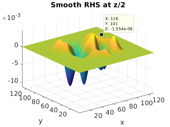
(a) Long-range part of charge density.

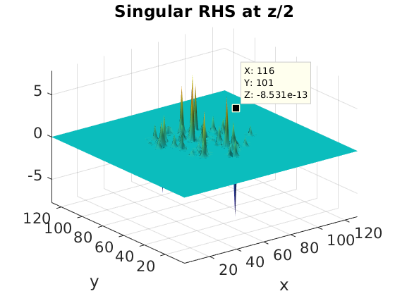
(b) Short-range part of charge density.

Figure 5.1: The long- and short-range parts of the charge density for protein Fasciculin 1 on $129^{\otimes 3}$ grid.

The nonlinear regularized PBE (NRPBE) can now be derived as follows. First, the unknown solution (or target electrostatic potential) $u$ to the PBE (2.1) can be decomposed as

$$u=u^{s}+u^{r},$$

where $u^{s}$ is the known singular function (or short-range component) and $u^{l}$ is the unknown long-range component to be determined. Therefore, the PBE (2.1) can be rewritten as

$$\left.\begin{aligned} \begin{aligned} -\nabla\cdot(\epsilon\nabla(u^{s}+u^{r}))+\bar{\kappa}^{2}\sinh(u^{s}+u^{r})&=f^{s}+f^{l}\quad\mbox{in}\,\,\mathbb{R}^{3},\\ u^{r}&=g,\quad\mbox{on}\quad\partial\Omega,\end{aligned}\end{aligned}\right\}$$ (5.6)

where the right-hand side of (2.1) is replaced by $f^{s}+f^{l}$ due to (5.2) and (5.4) and $g$ is the Dirichlet boundary conditions defined in (2.2).

It was proved in [3] and demonstrated in [1] that the function $f^{s}$ and the corresponding short-range potential $u^{s}$ are localized within the molecular region $\Omega_{m}$ and vanishes on the interface $\Gamma$. Moreover, from (2.3), the function $\bar{\kappa}$ is piecewise constant and $\bar{\kappa}=0$ in $\Omega_{m}$. Therefore, we can rewrite the Boltzmann distribution term in (5.6) as

$$\bar{\kappa}^{2}\sinh(u^{s}+u^{r})=\bar{\kappa}^{2}\sinh(u^{r}),\quad \mbox{ because }\,u^{s}=0\,\mbox{ in }\Omega_{s}.$$ (5.7)

Consequently, following the splitting of the Dirac delta distributions in (5.4), the short-range component of the potential satisfies the Poisson equation, i.e.,

$$-\nabla\cdot(\epsilon_{m}\nabla u^{s})=f^{s}\quad\mbox{in}\,\,\mathbb{R}^{3}.$$ (5.8)

It can be easily shown that

$$u^{s}(\bar{x})={\bf P}_{s}$$

is the cumulated canonical tensor in (3.12) which represents the precomputed short-range potential sum supported within the solute domain $\Omega_{m}$.

Subtracting (5.8) from (5.6) and using (5.7), we obtain the NRPBE as follows

$$-\nabla\cdot(\epsilon\nabla u^{r}(\bar{x}))+\bar{\kappa}^{2}(\bar{x})\sinh(u^{r}(\bar{x}))=f^{l},\quad\mbox{in}\,\,\,\Omega,$$ (5.9)

subject to

$$u^{r}(\bar{x})=\bar{\kappa}^{2}(\bar{x})\mathbf{P}_{l}\quad\mbox{on}\,\,\partial{\Omega}.$$ (5.10)

We recall that the regularization scheme for linear PBE introduced in [1] reads as follows,

$$-\nabla\cdot(\epsilon\nabla u^{r}(\bar{x}))+\bar{\kappa}^{2}(\bar{x})u^{r}(\bar{x})=f^{l}(\bar{x}),\,\mbox{in}\,\,\,\Omega,$$ (5.11)

subject to the Dirichlet boundary conditions

$$u^{r}(\bar{x})=\bar{\kappa}^{2}(\bar{x})\mathbf{P}_{l}\quad\mbox{on}\,\,\partial{\Omega}.$$ (5.12)

In this way, (5.9) – (5.10) generalizes the regularization scheme (5.11) – (5.12) to the nonlinear case.

Notice that by construction, the short-range potential vanishes on the interface $\Gamma$, hence it satisfies the discrete Poisson equation in (4.1) with the respective charge density $f^{s}$ and zero boundary conditions on $\Gamma$. Therefore, we recall (see [1] for the detailed discussion) that this equation can be subtracted from the full linear discrete PE system, such that the long-range component of the solution, $\mathbf{P}_{l}$, will satisfy the same linear system of equations (same interface conditions), but with a modified charge density corresponding to the weighted sum of the long-range tensors $f^{l}$ only.

6 Numerical approach to solving the NRPBE

Consider the uniform 3D $n^{\otimes 3}$ rectangular grid in $\Omega=[-b,b]^{3}$ with the mesh parameters $dx,dy,dz<0.5$. One standard way of solving the NRPBE in (5.9) is that it is first discretized in space to obtain a nonlinear system in matrix-vector form

$$A(u_{\mathcal{N}}^{r})=b^{r},\qquad\mbox{ in }\,\mathbb{R}^{\mathcal{N}},$$ (6.1)

where $A(u_{\mathcal{N}}^{r})\in\mathbb{R}^{\mathcal{N}\times\mathcal{N}}$, $b^{r}\in\mathbb{R}^{\mathcal{N}}$, and $u_{\mathcal{N}}^{r}$ is the discretized solution vector. Here, $\mathcal{N}$ is usually in $\mathcal{O}(10^{6})$.

Then system (6.1) can be solved using several existing techniques. For example, the nonlinear relaxation methods has been implemented in the Delphi software [45], the nonlinear conjugate gradient (CG) method has been implemented in University of Houston Brownian Dynamics (UHBD) software [46], the nonlinear multigrid (MG) method [47] and the inexact Newton method have been implemented in the adaptive Poisson-Boltzmann solver (APBS) software [48].

In this study, we apply a different approach of solving (5.9) [25, 49, 50]. In particular, an iterative approach is first applied to the continuous NRPBE in (5.9), where at the $(n+1)$st iteration step, the NRPBE is approximated by a linear equation via the Taylor series truncation. The expansion point of the Taylor series is the continuous solution $(u^{r})^{n}$ at the $n$th iteration step.

Consider $(u^{r})^{n}$ as the approximate solution at the $n$th iterative step, then the nonlinear term $\sinh((u^{r})^{n+1})$ at the $(n+1)$st step is approximated by its truncated Taylor series expansion as follows

$$\sinh((u^{r})^{n+1})\approx\sinh((u^{r})^{n})+((u^{r})^{n+1}-(u^{r})^{n})\cosh((u^{r})^{n}).$$ (6.2)

Substituting the approximation (6.2) into (5.9), we obtain

$$-\nabla\cdot(\epsilon(\bar{x})\nabla(u^{r})^{n+1})+\bar{\kappa}^{2}(\bar{x})\cosh((u^{r})^{n})(u^{r})^{n+1}=-\bar{\kappa}^{2}(\bar{x})\sinh((u^{r})^{n})\\ +\bar{\kappa}^{2}(\bar{x})\cosh((u^{r})^{n})(u^{r})^{n}+b^{r}.$$ (6.3)

The equation in (6.3) is linear, and can then be numerically solved by first applying spatial discretization. In this regard, we first define

$$\cosh\odot u_{\mathcal{N}}^{r}=:w=\begin{bmatrix}w_{1}\\ w_{2}\\ \vdots\\ w_{\mathcal{N}}\end{bmatrix},$$ (6.4)

where $\odot$ is the elementwise operation on a vector.

Then, we construct the corresponding diagonal matrix from (6.4) of the form

$$B=\mbox{diag}(w_{1},w_{2},\ldots,w_{\mathcal{N}}).$$

Finally, we obtain the following linear system

$$A_{1}(u_{\mathcal{N}}^{r})^{n+1}+A_{2}B^{n}(u_{\mathcal{N}}^{r})^{n+1}=-A_{2}\sinh\odot(u_{\mathcal{N}}^{r})^{n}+A_{2}B^{n}(u_{\mathcal{N}}^{r})^{n}+b_{1}^{r}+b_{2},$$ (6.5)

where $A_{1}$ is the Laplacian matrix and $A_{2}$ is a diagonal matrix containing the $\bar{\kappa}^{2}$ function. Note that the diagonal matrix $B^{n}$ changes at each iteration step, therefore, it cannot be precomputed. The vectors $b_{1}^{r}$ and $b_{2}$ are the regularized approximation of the Dirac delta distributions and the Dirichlet boundary conditions, respectively.

Let

$$A(\cdot)=A_{1}+A_{2}B^{n}$$ (6.6)

and

$$F:\mbox{right-hand side of}\>(\ref{eqn:Nonaffine_form_iterative_FOM}).$$ (6.7)

Then we obtain

$$A((u_{\mathcal{N}}^{r})^{n})(u_{\mathcal{N}}^{r})^{n+1}=F((u_{\mathcal{N}}^{r})^{n}),\quad n=0,1,\ldots.$$ (6.8)

Then, at each iteration, system (6.8) is a linear system w.r.t. $(u^{r}_{\mathcal{N}})^{n+1}$, which can be solved by any linear system solver of choice. In this study, we employ the aggregation-based algebraic multigrid method (AGMG) [51]. Algorithm 1 summarizes the detailed iterative approach of solving (6.8). This approach of first linearization, then discretization is shown to be more efficient than the standard way of first discretization and then linearization, via, for example, the Newton iteration. The advantage of the proposed approach is that it avoids computing the Jacobian of a huge matrix. It is observed that it converges faster than the standard Newton approach.

Algorithm 1 Iterative solver for the NRPBE

1:Initialize the potential $(u_{\mathcal{N}}^{r})^{0}$, e.g., $(u_{\mathcal{N}}^{r})^{0}=0$ and the tolerance $\delta^{0}=1$.

2:The converged NRPBE solution $(u_{\mathcal{N}}^{r})^{n}$ at $\delta^{n}\leq\tau$.

3:while $\delta^{n}\geq\tau$ do

4:     Solve the linear system (6.8) for $(u_{\mathcal{N}}^{r})^{n+1}$ using AGMG.

5:     $\delta^{n+1}\leftarrow\|(u_{\mathcal{N}}^{r})^{n+1}-(u_{\mathcal{N}}^{r})^{n}\|_{2}$.

6:     $(u_{\mathcal{N}}^{r})^{n}\leftarrow(u_{\mathcal{N}}^{r})^{n+1}$.

7:end while

The benefits of the RS tensor format as a solution decomposition technique over the existing techniques in the literature are highlighted as follows. First, the efficient splitting of the short- and long-range parts in the target tensor circumvents the need to modify jump conditions at the interface and the use of $\epsilon$ and $\bar{\kappa}$ as cut-off functions, e.g., in (4.6). Secondly, the long-range part in the RS tensor decomposition of the Dirac delta distributions [3] vanishes at the interface and, therefore, the modified charge density in (5.4) generated by this long-range component remains localized in the solute region. Thirdly, the boundary conditions are obtained from $\mathbf{P}_{l}$, the long-range part of the free space potential sum, thereby avoiding the computational costs involved in solving some external analytical function at the boundary. Lastly, only a single system of algebraic equations is solved for the regularized component of the collective potential which is then added to the directly precomputed short-range contribution, $u^{s}(\bar{x})$. This is more efficient than, for instance, in [24], where the regularized PBE model is subdivided into the linear interface and the nonlinear interface problems which are solved independently, with respective boundary and interface conditions.

7 Numerical results

In this section, we consider $n^{\otimes 3}$ 3D uniform Cartesian grids in a box $[-b,b]^{3}$ with equal step size $h=2b/(n-1)$ for computing the electrostatic potentials of the PBE on a modest PC with the following specifications: Intel (R) Core (TM) $i7-4790$ CPU @ 3.60GHz with 8GB RAM. The FDM is used to discretize the PBE in this work and the numerical computations are implemented in the MATLAB software, version R2017b.

7.1 Numerical results for LPBE

First, we validate our FDM solver for the classical LPBE by comparing its solution with that of the APBS software package (version 1.5-linux64), which uses the multigrid (PMG) accelerated FDM [43]. Here, we consider the protein Fasciculin 1, with 1228 atoms. Figure 7.1 shows the electrostatic potential of the PBE on a $n\times n$ grid surface with $n=129$ at the cross-section of the volume box ($60\,\mbox{\AA}$) in the middle of the $z$-axis computed by the FDM solver and the corresponding error between the two solutions. Here, we use the ionic strength of $0.15M$ and the dielectric coefficients $\epsilon_{m}=2$ and $\epsilon_{s}=78.54$, respectively. The numerical results show that the FDM solver provides as accurate results as those of the APBS with a discrete $L_{2}$ error of $\mathcal{O}(10^{-4})$ in the full solution.

(a) LPBE solution by the FDM solver.

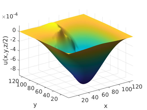
(b) APBS vs FDM solution error.

Figure 7.1: The electrostatic potential for the protein Fasciculin 1 computed by the FDM solver (left) and the error between the APBS and FDM solutions (right) on $129^{\otimes 3}$ grid, at $0.15M$ ionic strength.

The corresponding electrostatic potential energy for the aforementioned LPBE solvers on a sequence of fine grids is given in the Table 7.1. The results for solvation free energy of protein varieties are presented in [34]. To validate the claim in Remark 1, we provide in the Table 7.2, the comparison between the total electrostatic potential energies $\Delta G_{elec}$ in kJ/mol, between the LPBE and the nonlinear PBE (NPBE) computations on a sequence of fine grids using the APBS software package.

$h$	$\mathcal{N}$	$\Delta G_{elec}$, FDM	$\Delta G_{elec}$, APBS	Relative error
0.465	$129^{3}$	91,232.9217	91,228.0388	5.3524e-5
0.375	$161^{3}$	130,611.0021	130,606.0444	3.7962e-5
0.320	$193^{3}$	170,159.4204	170,154.3821	2.9610e-5

Table 7.1: Comparison of the total electrostatic potential energies $\Delta G_{elec}$ in kJ/mol, between FDM and APBS on a sequence of fine grids.

Remark 1

We reiterate that the solutions obtained from the LPBE and the nonlinear PBE are very close to each other, even when the linearization condition does not hold [4]. This is especially manifested in protein molecules whose charge densities are small. However, in biomolecules with large charge densities, for example, the DNA, significant differences might be observed at the solute-solvent interface [36, 4]. Moreover, the solution of the LPBE is usually used as the initial guess for the nonlinear PBE.

$h$	$\mathcal{N}$	$\Delta G_{elec}$, LPBE	$\Delta G_{elec}$, NPBE	Relative error
0.465	$129^{3}$	91,228.0575	91,227.8354	2.4345e-6
0.375	$161^{3}$	130,606.0630	130,605.8448	1.6707e-6
0.320	$193^{3}$	170,154.4401	170,154.1862	1.4922e-6

Table 7.2: Comparison of the total electrostatic potential energies $\Delta G_{elec}$ in kJ/mol, between the LPBE and the NPBE computations on a sequence of fine grids.

Remark 2

Notice from Table 7.1 and Table 7.2 that the electrostatic potential energies $\Delta G_{elec}$ increase with decreasing grid/mesh size, $h$. This is caused by the short-range electrostatic potential behaviour in $1/\|\bar{x}\|$ as $\|\bar{x}\|$ $\to 0$.

7.2 Accuracy of the nonlinear RPBE based on the RS tensor format

Here, we provide the results for the calculation of electrostatic potential for the nonlinear RPBE (NRPBE) based on the RS tensor format and compare the results with those of the traditional NPBE for various proteins. First, we consider the protein Fasciculin 1 consisting of 1228 atoms of varying atomic radii as shown in Table 7.3. Notice that 322 of the total atoms have zero radius, which implies that we must annihilate them from the RS tensor format calculations so that they are not assigned Newton kernels. Therefore, we consider the smallest atom in the protein as that with 1 Å radius, (i.e., the Hydrogen atom).

Atomic radii in Å
Atomic radius	0.00	1.00	1.40	1.50	1.70	1.85	2.00
Number of atoms	322	333	195	82	104	10	182

Table 7.3: Atomic radii and the corresponding number of atoms for the constituent atoms of the protein Fasciculin 1.

We provide the comparisons between the electrostatic potential computed by the NRPBE, based on the RS tensor format, with that of the traditional NPBE. Figure 7.2 shows the solutions from the two models and the corresponding error on $129^{\otimes 3}$ uniform Cartesian grid and a $60\mbox{\AA}$ domain length, at $0.15M$ ionic strength.

Remark 3

Notice that the error is predominant within the molecular region, where the solution is singular. However, in the solute region, which is dominated by the long-range regime, the error is small, of order $\mathcal{O}(10^{-5})$.

Figure 7.2: Absolute error between the solutions of the traditional NPBE and the NRPBE for the protein Fasciculin 1.

Figure 7.3 provides the cross-sectional view of the electrostatic potential shown in Figure 7.2, for demonstrating the accuracy of the numerical treatment of the solution singularities inherent in the NRPBE model as compared with the traditional NPBE model. Notice that the NRPBE is capable of capturing exactly, the short-range component of the total potential sum because this part is precomputed analytically thereby avoiding the numerical errors generated by the traditional NPBE solver.

Remark 4

Figure 3(b) contains densely populated singularities/cusps as a result of explicit treatment of each atomic charge by the short-range part of the RS tensor whereas Figure 3(a), displays sparsely populated singularities, most of which are not sharp due to the redundant smoothing/smearing effect of the atomic charges by the cubic spline interpolation.

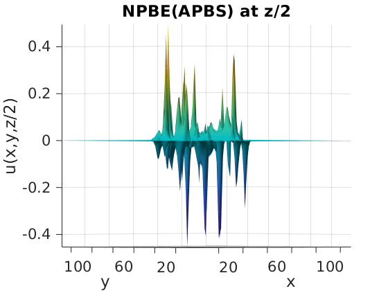
(a) Cross-sectional view of NPBE solution in Figure 7.2.

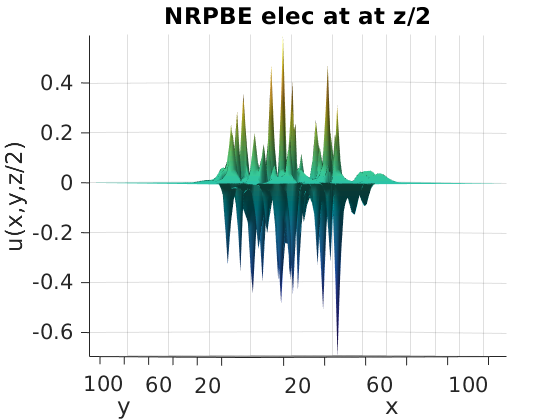
(b) Cross-sectional view of NRPBE solution in Figure 7.2.

Figure 7.3: The cross-sectional view of the electrostatic potentials in Figure 7.2.

Secondly, we provide results for a 180-residue cytokine solution NMR structure of a murine-human chimera of leukemia inhibitory factor (LIF) [52] consisting of 2809 atoms. The corresponding variation in atomic radii and the corresponding atomic occurrences are shown in Table 7.4. Figure 7.4 shows the comparison between the electrostatic potential of NRPBE, with that of the classical NPBE and the corresponding error on a $129^{\otimes 3}$ grid and a $65\mbox{\AA}$ domain length, at $0.15M$ ionic strength.

Atomic radii in Å
Atomic radius	0.2245	0.4500	0.9000	1.3200	1.3582	1.4680	$\geq$ 1.7000
Number of atoms	315	6	6	1032	54	6	1390

Table 7.4: Atomic radii and the corresponding number of atoms for the constituent atoms of a 180-residue cytokine solution NMR structure of a murine-human chimera of leukemia inhibitory factor (LIF).

Figure 7.4: Absolute error between the solutions of the traditional NPBE and the NRPBE for the murine-human chimera of leukemia inhibitory factor (LIF).

Remark 5

In a similar vein, we notice in Figure 7.5 that the error is predominant within the molecular region, where the solution is singular. It is also worth mentioning that the small atomic radii, ($<0.9\mbox{\AA}$), in Table 7.4 are treated independently in terms of the RS tensor splitting of the short- and long-range potentials.

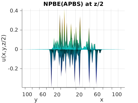
(a) Cross-sectional view of NPBE solution in the Figure 7.2.

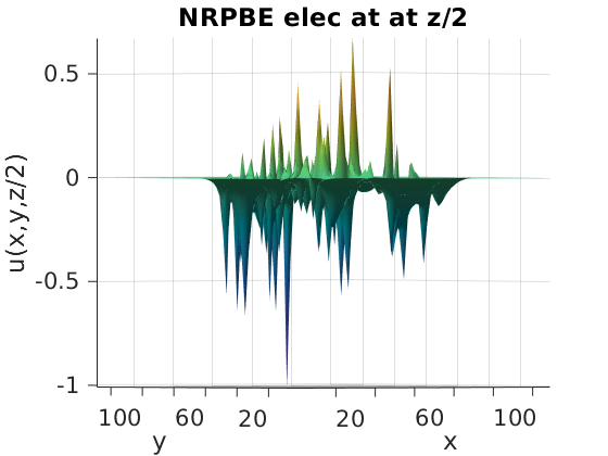
(b) Cross-sectional view of NRPBE solution in the Figure 7.2.

Figure 7.5: The cross-sectional view of the electrostatic potentials in the Figure 7.4.

7.3 Runtimes and Computational Speed-ups

We compare the runtimes of computing both the classical and regularized PBE models in Table 7.5 for the protein Fasciculin 1 in an $n^{3}=129^{3}$ domain of $60\,\mbox{\AA}$ length at an ionic strength of $0.15M$. Notice that the runtimes for the LPBE and the LRPBE are almost equal because the linear systems are solved by the same solver (i.e., AGMG). On the other hand, the runtime for solving the nonlinear system for the NRPBE is half that of the NPBE due to the absence of the Dirac delta distributions and their corresponding solution singularities in our scheme, and which increase the computational costs in NPBE.

Runtime (seconds) and speed-up
	LPBE	LRPBE	Speed-up
Solve linear system	5.26	6.34	$\approx$ 1
Total runtime	15.25	16.47	$\approx$ 1
	NPBE	NRPBE	Speed-up
Solve nonlinear system	24.23	12.30	1.97
Total runtime	34.40	28.30	1.21

Table 7.5: Runtimes and speed-ups for LPBE, LRPBE, NPBE, and NRPBE.

8 Conclusions

In this paper, we apply the RS tensor format for a solution decomposition of the nonlinear PBE for computation of electrostatic potential of large solvated biomolecules. The efficacy of the tensor-based regularization scheme established in [1] for the linear PBE, is based on the unprecedented properties of the grid-based RS tensor splitting of the Dirac delta distribution [3]. Similar to the linear case, the key computational benefits are attributed to the localization of the modified Dirac delta distributions within the molecular region and the automatic maintaining of the continuity of the Cauchy data on the solute-solvent interface. Moreover, our computational scheme entails solving only a single system of algebraic equations for the regularized component of the collective electrostatic potential discretized by the FDM. The total potential is obtained by adding this solution to the directly precomputed low-rank tensor representation of the short-range contribution.

The main properties of the presented scheme are demonstrated by various numerical tests. For instance, Figure 7.3 and Figure 7.5 vividly demonstrate that the traditional PBE model does not accurately capture the solution singularities which originate from the short-range component of the total target electrostatic potential in the numerical approximation. In the RPBE, the Dirac delta distribution is replaced by a smooth long-range function from (5.4). It only requires one to solve for the long-range electrostatic potential numerically and add this solution to the short-range component which is computed a priori using the canonical tensor approximation to the Newton kernel. The resultant total potential sum is of high accuracy as demonstrated by Figure 3(b) and Figure 5(b).

References

- Benner et al. [2021] P. Benner, V. Khoromskaia, B. Khoromskij, C. Kweyu, and M. Stein. Regularization of Poisson-Boltzmann type equations with singular source terms using the range-separated tensor format. SIAM J. Sci. Comput., 43(1):A415–A445, 2021. doi: 10.1137/19M1281435.
- Benner et al. [2018] P. Benner, V. Khoromskaia, and B. N. Khoromskij. Range-separated tensor format for many-particle modeling. SIAM J. Sci. Comp., (2):A1034–A1062, 2018.
- Khoromskij [2018] B. N. Khoromskij. Range-separated tensor representation of the discretized multidimensional Dirac delta and elliptic operator inverse. Preprint, arXiv:1812.02684v1, 2018.
- Fogolari et al. [2002] F. Fogolari, A. Brigo, and H. Molinari. The Poisson-Boltzmann equation for biomolecular electrostatics: a tool for structural biology. J. Mol. Recognit., 15(6):377–392, 2002. doi: 10.1002/jmr.577.
- Neves-Petersen and Petersen [2003] M. T. Neves-Petersen and S. Petersen. Protein electrostatics: A review of the equations and methods used to model electrostatic equations in biomolecules - applications in biotechnology. Biotechnol. Annu. Rev., 9:315–395, 2003. doi: 10.1016/S1387-2656(03)09010-0.
- Gabdoulline et al. [2007] R. R. Gabdoulline, M. Stein, and R. C. Wade. qPIPSA: relating enzymatic kinetic parameters and interaction. BMC Bioinformatics, 8:373:1–16, 2007.
- Stein et al. [2010] M. Stein, R. R. Gabdoulline, and R. C. Wade. Cross-species analysis of the glycoliticmpathway by comparison of molecular interaction fields. Molecular Biosystems, 6:162–174, 2010.
- Deserno and Holm [1998] M. Deserno and C. Holm. How to mesh up Ewald sums. I. A theoretical and numerical comparison of various particle mesh routines. J. Chem. Phys., 109(18):7678–7693, 1998.
- Lipparini et al. [2013] F. Lipparini, B. Stamm, E. Cances, Y. Maday, and B. Mennucci. Domain decomposition for implicit solvation models. J. Chem. Theor. Comp., 9:3637–3648, 2013.
- Ren et al. [2012] P. Ren, J. Chun, D.G. Thomas, M.J. Schnieders, M. Marucho, J. Zhang, and N.A. Baker. Biomolecular electrostatics and solvation: a computational perspective. Quarterly Reviews of Biophysics, 45(4):427–491, 2012. doi: 10.1017/S003358351200011X.
- Jurrus et al. [2017] E. Jurrus, D. Engel, K. Star, K. Monson, J. Brandi, L.E. Felberg, D.H. Brookes, L. Wilson, J. Chen, K. Liles, M. Chun, P. Li, D.W. Gohara, T. Dolinsky, R. Konecny, D.R. Koes, J.E. Nielsen, T. Head-Gordon, W. Geng, R. Krasny, G.W. Wei, M.J. Holst, J.A. McCammon, and N.A. Baker. Improvements to the apbs biomolecular solvation software suite. Protein Science, 27(1):112–128, 2017. doi: 10.1002/pro.3280.
- D. and D.A. [2000] Bashford D. and Case D.A. Generalized Born models of macromolecular solvation effects. Annu. Rev. Phys. Chem., 51:129–152, 2000.
- Kweyu et al. [2022] C. Kweyu, L. Feng, M. Stein, and P. Benner. Reduced basis method for the nonlinear Poisson–Boltzmann equation regularized by the range-separated canonical tensor format. International Journal of Nonlinear Sciences and Numerical Simulation, pages 2191–0294, 2022. doi: 10.1515/ijnsns-2021-0103.
- V. et al. [1997] Barone V., Cossi M., and Tomasi J. A new definition of cavities for the computation of solvation free energies by the polarizable continuum model. J. Chem. Phys., 107:3210–3221, 1997.
- Holst [1994] M. J. Holst. Multilevel methods for the Poisson-Boltzmann equation. Ph.D. Thesis, Numerical Computing group, University of Illinois, Urbana-Champaign, IL, USA, 1994.
- Dong et al. [2008] F. Dong, B. Oslen, and N. A. Baker. Computational methods for biomolecular electrostatics. Methods Cell Biol, 84(1):843–870, 2008. doi: 10.1016/S0091-679X(07)84026-X.
- Warwicker and Watson [1982] J. Warwicker and H. C. Watson. Calculation of the electric potential in the active site cleft due to -helix dipoles. J. Mol. Biol., 157(4):671–679, 1982. doi: 10.1016/0022-2836(82)90505-8.
- Baker et al. [2001a] N. A. Baker, M. J. Holst, and F. Wang. The adaptive multilevel finite element solution of the Poisson-Boltzmann equation on massively parallel computers. IBM J. Res. Devel., 45:427–438, 2001a.
- Wang and Luo [2010] J. Wang and R. Luo. Assessment of linear finite difference Poisson-Boltzmann solvers. J. Comput. Chem., 31:1689–1698, 2010. doi: 10.1016/j.cpc.2015.08.029.
- Holst et al. [2000] M. Holst, N. Baker, and F. Wang. Adaptive multilevel finite element solution of the Poisson-Boltzmann equation: algorithms and examples. J. Comp. Chem., 21:1319–1342, 2000. doi: 10.1002/1096-987X(20001130)21:15¡1319::AID-JCC1¿3.0.CO;2-8.
- Boschitsch and Fenley [2004] A. H. Boschitsch and M. O. Fenley. Hybrid boundary element and finite difference method for solving the nonlinear Poisson-Boltzman equation. J. Comput. Chem., 25(7):935–955, 2004. doi: 10.1002/jcc.20000.
- Zhou [1993] H. X. Zhou. Boundary element solution of macromolecular electrostatics: Inteaction energy between two proteins. Biophys. J., 65(2):955–963, 1993. doi: 10.1016/S0006-3495(93)81094-4.
- Lu et al. [2008] B. Z. Lu, Y. C. Zhou, M. J. Holst, and J. A. McCammon. Recent progress in numerical methods for Poisson-Boltzmann equation in biophysical applications. Commun. Comp. Phys., 3(5):973–1009, 2008.
- Xie [2014] D. Xie. New solution decomposition and minimization scheme for Poisson-Boltzmann equation in calculation of biomolecular electrostatics. J Comp. Phys., 275:294–309, 2014.
- Mirzadeh et al. [2013] M. Mirzadeh, M. Theillard, A. Helgadottir, D. Boy, and F. Gibou. An adaptive, finite difference solver for the nonlinear Poisson-Boltzmann equation with applications to biomolecular computations. Commun. Comput. Phys., 13(1):150–173, 2013. doi: 10.4208/cicp.290711.181011s.
- Chen et al. [2007] L. Chen, M.J. Holst, and J. Xu. The finite element approximation of the nonlinear Poisson-Boltzmann equation. SIAM J. Numer. Anal., 45(6):2298–2320, 2007. doi: 10.1137/060675514.
- Chern et al. [2003] I. Chern, J. Liu, and W. Wang. Accurate evaluation of electrostatics for macromolecules in solution. Methods Appl. Anal., 10(2):309–328, 2003.
- Benner et al. [2016] P. Benner, V. Khoromskaia, and B. N. Khoromskij. Range-separated tensor formats for numerical modeling of many-particle interaction potentials. arXiv:1606.09218v3, pages 1–38, 2016.
- Badreddine et al. [2022] S. Badreddine, I. Chollet, and L. Grigori. Factorized structure of the long-range two-electron integrals tensor and its application in quantum chemistry. arXiv:2210.13069, 2022.
- Bertoglio and Khoromskij [2012] C. Bertoglio and B. N. Khoromskij. Low-rank quadrature-based tensor approximation of the Galerkin projected Newton/Yukawa kernels. Comp. Phys. Comm., 183(4):904–912, 2012. doi: 10.1016/j.cpc.2011.12.016.
- Khoromskij and Khoromskaia [2009] B. N. Khoromskij and V. Khoromskaia. Multigrid accelerated tensor approximation of function related multidimensional arrays. SIAM J. Sci. Comp., 31(4):3002–3026, 2009. doi: 10.1137/080730408.
- Khoromskaia and Khoromskij [2018] V. Khoromskaia and B.N. Khoromskij. Tensor numerical methods in quantum chemistry. De Gruyter, Berlin, 2018.
- Khoromskaia and Khoromskij [2014] V. Khoromskaia and B. N. Khoromskij. Grid-based lattice summation of electrostatic potentials by assembled rank-structured tensor approximation. Comp. Phys. Comm., 185(12), 2014.
- Benner et al. [2017] P. Benner, L. Feng, C. Kweyu, and M. Stein. Fast solution of the poisson-boltzmann equation with nonaffine parametrized boundary conditions using the reduced basis method. arXiv:1705.08349, 221, 2017.
- Sharp and Honig [1990] K. A. Sharp and B. Honig. Electrostatic interactions in macromolecules: theory and applications. Annu. Rev. Biophys. Chem., 19:301–332, 1990.
- Fogolari et al. [1999] F. Fogolari, P. Zuccato, G. Esposito, and P. Viglino. Biomolecular electrostatics with the linearized Poisson-Boltzmann equation. Biophys. J., 76(1):1–16, 1999. doi: 10.1016/S0006-3495(99)77173-0.
- Wade et al. [2001] R.C. Wade, R.R. Dabdoulline, and F. De Rienzo. Protein interaction property similarity analysis. International Journal of Quantum Chemistry, 83:122–127, 2001.
- Khoromskij et al. [2011] B. N. Khoromskij, V. Khoromskaia, and H.-J. Flad. Numerical solution of the Hartree-Fock equation in multilevel tensor-structured format. SIAM J. Sci. Comp., 33(1):45–65, 2011.
- Khoromskaia and Khoromskij [2007] V. Khoromskaia and B. N. Khoromskij. Low rank Tucker tensor approximation to the classical potentials. Centr. Europ. J. Math., 5(3):1–28, 2007.
- Hackbusch and Khoromskij [2006] W. Hackbusch and B.N. Khoromskij. Low-rank Kronecker product approximation to multi-dimensional nonlocal operators. part I. Separable approximation of multi-variate functions. Computing, 76:177–202, 2006.
- Khoromskij [2006] B. N. Khoromskij. Structured rank- decomposition of function-related operators in . Comp. Meth. Appl. Math, 6(2):194–220, 2006.
- Khoromskaia et al. [2012] V. Khoromskaia, B. N. Khoromskij, and D. Andrae. Fast and accurate 3D tensor calculation of the Fock operator in a general basis. Comp. Phys. Comm., 183(11), 2012.
- Baker et al. [2001b] N. A. Baker, D. Sept, S. Joseph, M. J. Holst, and J. A. McCammon. Electrostatics of nanosystems: application to microtubules and the ribosome. Proc. Nat. Acad. Sci. U.S.A., 98(18):10037–10041, 2001b. doi: 10.1073/pnas.181342398.
- le Du et al. [1992] M.H. le Du, P. Marchot, P.E. Bougis, and J.C. Fontecilla-Camps. 1.9 Angstrom resolution structure of fasciculine 1, an anti-acetylcholinesterase toxin from green mamba snake venom. J. Biol. Chem., 267:22122–22130, 1992.
- Rocchia et al. [2001] W. Rocchia, E. Alexov, and B. Honig. Extending the applicability of the nonlinear Poisson-Boltzmann equation: multiple dielectric constants and multivalent ions. J. Phys. Chem., 105(28):6507–6514, 2001. doi: 10.1021/jp010454y.
- Luty et al. [1992] B.A. Luty, M.E. Davis, and J.A McCammon. Solving the finite-difference nonlinear Poisson-Boltzmann equation. J. Comput. Chem., 13(9):1114–1118, 1992. doi: 10.1002/jcc.540130911.
- Oberoi and Allewell [1993] H. Oberoi and N. M. Allewell. Multigrid solution of the nonlinear Poisson-Boltzmann equation and calculation of titration curves. Biophys. J., 65(1):48–55, 1993. doi: 10.1016/S0006-3495(93)81032-4.
- Holst and Saied [1995] M. Holst and F. Saied. Numerical solution of the nonlinear Poisson-Boltzmann equation: Developing more robust and efficient methods. J. Comput. Chem., 16:337–364, 1995.
- Shestakov et al. [2002] A. I. Shestakov, J. L. Milovich, and A. Noy. Solution of the nonlinear Poisson-Boltzmann equation using pseudo-transient continuation and the finite element method. Commun. Comput. Phys., 247:62–79, 2002. doi: 10.1006/jcis.2001.8033.
- Ji et al. [2019] L. Ji, Y. Chen, and Z. Xu. A reduced basis method for the nonlinear Poisson-Boltzmann equation. Adv. Appl. Math. Mech., 11:1200–1218, 2019. doi: 10.4208/aamm.OA-2018-0188.
- Notay [2010] Y. Notay. An aggregation-based algebraic multigrid method. Electronic Transactions on Numerical Analysis, 37:123–146, 2010.
- Hinds et al. [1998] M.G. Hinds, T. Maurer, Zhang J., and N.A. Nicola. Solution structure of Leukemia inhibitory factor. BiolChem, 273:13738–13745, 1998. doi: 10.1074/jbc.273.22.13738.