Correlation between normal and superconducting states within the Fermi-liquid region of the T-p phase diagram of quantum-critical heavy-Fermion superconductors

Abstract

Extensively reported experimental observations indicate that on varying pressure ($p$) within the T-p phase diagram of most quantum critical heavy fermion (HF) superconductors, one identifies a cascade of distinct electronic states which may be magnetic, of Kondo-type, non-conventional superconducting, Fermi Liquid (FL), or non-FL character. Of particular interest to this work is the part of the phase diagram lying below a specific phase boundary, $T^{*}_{\text{{FL}}}(p^{*})$, across which the transport and thermodynamic properties switch over from non-FL into FL behavior. Remarkably, this nontrivial manifestation of FL phase is accompanied by (i) the characteristic $\rho_{o}+\textit{AT}^{2}$ dependence ($\rho_{o}$ = residual resistivity), (ii) a superconductivity below $T_{c}\leq T^{*}_{\text{{FL}}}(p^{*})$, and (iii) a universal scaling of $T_{c}$ and $A$: $ln\frac{T_{c}}{\theta}\propto A^{-\frac{1}{2}}$ ($\theta$ = characteristic energy scale). We consider that such features are driven by a fluctuation-mediated electron-electron scattering channel with the mediating quasiparticles being either spin fluctuations [Mathur et al. Nature 394, 39 (1998)] or valence fluctuations [Miyake and Watanabe, Phil. Mag.97, 3495–3516 (2017)] depending on the character of the neighboring instability. On adopting such a scattering channel and applying standard theories of Migdal-Eliashberg (superconductivity) and Boltzmann (transport), we derive analytic expressions that satisfactorily reproduce the aforementioned empirical correlations in these heavy fermion superconductors.

I Introduction

There is ongoing interest in investigating the correlations between the normal-state and superconducting properties of heavy fermion (HF) superconduconductors when subjected to a variation in a nonthermal control parameter such as pressure $p$, concentration of charge carriers $n$, stoichiometry/doping $x$, disorder, or magnetic field $H$.^{1; 2; 3; 4; 5} Driven by ease and convenience, the evolution of these correlations is often investigated within a T-p phase diagram; there, an extrapolation of the phase boundaries down to zero temperature often leads to one or two quantum critical/crossover points.^{1; 2; 3; 4; 5; 6; 7} One is usually attributed to a magnetic instability at $p_{m}$; often, it is accompanied by a superconducting dome wherein the superconductivity is considered to be driven by spin fluctuations.⁶ The other point, at $p_{v}$, is usually assigned to a valence instability⁷ which, as well, is often accompanied by a superconducting dome with the superconductivity considered to be driven by valence fluctuations.^{8; 7}

A surge of superconducting dome within the neighborhood of a magnetic quantum critical point is also manifested in other superconducting family, such as high-Tc cuprates and Fe-based pnictides and chalcogenides.^{9; 10} Much of the understanding of the superconducting and normal-state properties were obtained from theoretical and experimental investigation of three regions of the dome: the two neighboring the emergence and disappearance of the superconductivity (at the left and right $T_{c}\rightarrow 0$) while the third is at the middle wherein $T_{c}$ is a maximum. Analysis of the character of the left and middle regions is usually complicated by the additional influence of competing antiferromagnetic, spin glass, charge and stripes, or pseudogap phases. In contrast, investigation of the region at the right $T_{c}\rightarrow 0$ limit is much simpler since only two states are involved, namely the superconducting and the FL phases.^{11; 12; 13; 14; 15} This work, in line with Refs. ¹¹; ¹²; ¹³; ¹⁴; ¹⁵, investigate the evolution of (and correlation among) the superconducting and normal states within the FL region of the HF T-p phase diagram. As shown below, in contrast to these references, (i) we consider explicitly the normal-state FL character, (ii) we do not invoke any additional impurity scattering; rather we consider the spin-fluctuations to be operating within patches of the sample (the average dimension of a patch is longer than the mean free path and coherent length while their concentration is reflected in the excess residual resistivity), and most importantly (iii) we consider that the very same fluctuation-mediated electron-electron scattering channel is responsible for the evolution of both the superconductivity and the FL character.

It is worth recalling that various experiments reveal the presence of phase-boundary curve, e.g. $T^{*}_{\text{{FL}}}(p^{*})$ within the HF T-p phase diagram, across which both the transport and thermodynamic properties switch over from non-Fermi-liquid (NFL) into a Fermi-liquid (FL) behavior. Such a switch is best illustrated by the electronic contribution to the low-temperature resistivity, $\rho(T,p)$, of typical HF superconductors: Within the NFL phase,

$$\rho(T>T^{*}_{\text{{FL}}}[p^{*}],p\leq p^{\text{*}})-\rho_{x}=\rho_{\circ}+A_{\text{NFL}}T^{n},\mathrm{\,\,\,\,\,\,[n<2],}$$ (1)

while within the FL phase,

$$\rho(T_{c}<T<T^{*}_{\text{FL}}[p^{*}],p>p^{\text{*}})-\rho_{x}=\rho_{\circ}+AT^{2},$$ (2)

where $\rho_{x}=\rho_{\circ}^{n.f.}+\rho_{n.f.}(T)$ represents all non-fluctuation-related (e.g. defects, phonon, magnetic) contributions (see end of Subsec. II.1). Within the FL region (which starts at the switching of NFL into FL character and ends when $T_{c}\rightarrow 0$), we denote the excess contribution of the residual resistivity by $\rho_{\circ}$, that of the quadratic-in-T coefficient by $A$, and that of the superconductivity transition by $T_{c}$; all these contributions are attributed to a fluctuation-mediated electron-electron (e-e) scattering channel (see below). Generally, these $\rho_{\circ}(p),\,A(p),$ and $T_{c}(p)$ parameters —  derived from experimental $\rho(T,p)$ curves —manifest a dramatic and non-monotonic variation around each of the critical $p_{m}$ and $p_{v}$ points (see, e.g., Figs. 2,3,4).

In this work, we are interested in analyzing and rationalizing the baric evolution of $\rho_{\circ}(p)$, $A(p)$, and $T_{c}(p)$ within the FL region of various archetype HF superconductors. Our analysis identified two universal correlations among these $\rho_{\circ}$, $A$, and $T_{c}$ parameters. We argue that the fluctuation-mediated electron-electron scattering channel is responsible for the emergence of the superconductivity, the FL character and the correlations among them.

The text below is organized as follows. We first recall some helpful insight regarding the fluctuation-mediated e-e scattering process.^{6; 7} In Subsec. II.2 we extract, identify, and generalize two main empirical correlations. In Subsec. II.3 we argue that these correlations are driven by a fluctuation-mediated e-e interaction channel. Such fluctuations can be either spin fluctuation⁶ or valence fluctuation⁷ (generically referred to as fluctuation). Although we consider below the spin-fluctuation exchange mechanism ⁶, generalization to valence fluctuation⁷ is implicitly assumed. On adopting such a mechanism and applying standard Migdal-Eliashberg description of superconductivity and Boltzmann’s transport theory, we derive analytic expressions that compare favorably with the empirically-obtained correlations. Comparison to other fluctuation-bearing/defect-bearing superconductors will be briefly discussed in Sec. III; there, we demonstrate the generality of our approach by discussing the Kadowaki-Woods and gap-to-$T_{c}$ ratios of these HF superconductors.

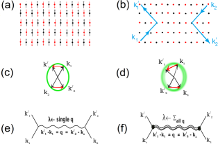
Figure 1: A sketch of a fluctuation-mediated e-e interaction channel. (a) An antiferromagnet structure representing an initial state in the phase diagram of a typical heavy fermion superconductor. The tiny arrows denote localized magnetic moments of atomic entities (represented by the small solid circles). (b) The nonmagnetic state after the quench of localized magnetic moments and, consequently, the magnetic structure. Within the direct lattice, the two electrons with ${\bf k}_{1}$ and ${\bf k}_{2}$ scatter into final states ${\bf k}_{1}^{\prime}$ and ${\bf k}_{2}^{\prime}$. (c) A $\bf{\delta g}=0$ two-electrons scattering process in the reciprocal space: As that ${\bf q}={\bf k}_{1}^{\prime}-{\bf k}_{1}-{\bf g}$, the phase space for scattering is quite limited; a Fermi-liquid sate is possible only at very low temperatures. (d) The $\bf{\delta g}\neq 0$ two-electrons scattering process in the reciprocal space: as that ${\bf q}={\bf k}_{1}^{\prime}-{\bf k}_{1}-{\bf g}-\delta{\bf g}$, the phase space available for scattering is considerably enlarged, leading to a robust superconducting and Fermi-liquid states. (e) Feynman diagram of the $\bf{\delta g}=0$ process [as in panel (c)] wherein only longitudinal modes are involved. (f) The Feynman diagram of the $\bf{\delta g}\neq 0$ process [as in panel (d)] which is mediated by exchanging all kinematically unconstrained modes.

II Analysis

II.1 Some Preliminaries on the fluctuation-mediated e-e interaction channel

It is recalled that a typical T-p phase diagram of most quantum-critical HF superconductors exhibits a series of distinct electronic states (see, e.g., Figs. 2(a)-3(a) and Refs. [³; ⁸; ¹⁶]). Often, the initial state is an antiferromagnetic, represented in Fig. 1(a) as simple two-dimension Neel-type arrangment. Beyond a critical value of the control parameter, $p_{m}$ in the present cases, the localized moments and the three-dimensional magnetic structure are quenched leading to a series of "nonmagnetic" states which can be of Kondo-type, non-conventional superconducting, non-FL, or FL character. Nevertheless, some remnant magnetic fluctuations persist within various micro-sized patches which are distributed randomly within an otherwise metallic matrix.¹⁷

These magnetic fluctuations are considered to mediate an e-e scattering process ⁶: as shown in Figs. 1(b-f), the two electrons with ${\bf k}_{1}$ and ${\bf k}_{2}$ scatter into final states ${\bf k}_{1}^{\prime}$ and ${\bf k}_{2}^{\prime}$. In particular, the electron, initially at a state ${\bf k}_{1}$, goes into a final state ${\bf k}_{1}^{\prime}$ after being scattered by a mode with wavevector ${\bf q}$; in doing so, it transfers an amount of energy and quasi-momentum satisfying ${\bf k}_{1}^{\prime}-{\bf k}_{1}-{\bf q}={\bf g}+\bf{\delta g}$ where ${\bf g}$ is a vector in a reciprocal magnetic lattice while $\bf{\delta g}$ is an uncertainty in ${\bf g}$ due to the inherent nature of the process leading to fluctuation (most obvious for the doping process).

We consider that, within the Fermi-liquid state of these HF superconductors, an increase in pressure leads to a reduction of the size and density of the fluctuation-bearing patches,¹⁷ till eventually one reaches, at very high pressure, the fluctuation-free state wherein no modes are available for mediation. This, as will be detailed below in Figs. 2, 3, and 4, leads to a complete removal of fluctuation-related features, namely the superconductivity ($T_{c}\rightarrow 0$), the Fermi-liquid state ($A\rightarrow A_{\circ}$), the residual resistivity ($\rho\rightarrow\rho_{\circ}^{\circ}$), and their correlations.

Let us now discuss the fluctuation-based mediation within the FL region. First, we consider the case satisfying $\bf{\delta g}=0$ condition of Figs. 1(c) and 1(e). Here, the quasi-momentum ${\bf q}={\bf k}_{1}^{\prime}-{\bf k}_{1}-{\bf g}$ is conserved exactly. Accordingly, only longitudinal modes with a well defined polarization, $\hat{{\bf e}}({\bf q}={\bf k}_{1}^{\prime}-{\bf k}_{1})$, will be involved. This means that the phase space available for momentum relaxation will be quite limited leading to, if any, a very small $T_{c}$ and $A$.

Secondly, in contrast to above, the surge of fluctuation-based mediation satisfying ${\bf\delta g}\neq 0$ condition, Figs. 1(d) and 1(f), provides a source for short wavelength (large ${\bf q}$) phase interference. This $\bf{\delta g}\neq 0$ condition implies that the quasi-momentum ${\bf q}={\bf k}_{1}^{\prime}-{\bf k}_{1}-{\bf g}-\delta{\bf g}$ is no longer conserved since $\bf{\delta g}$ is arbitrary.^{18; 19; 20} Then, multiple modes [longitudinal and transverse, of all polarizations $\hat{{\bf e}}({\bf q}\neq{\bf k}_{1}^{\prime}-{\bf k}_{1}-{\bf g})$] become kinematically available, Fig. 1(f). As shown in Fig. 1(d), the phase space available for momentum relaxation is considerably enlarged: this leads to an enhanced $T_{c}$ and $A$.

Considering the above partitioning of a fluctuation-bearing sample into two spacial regions, Matthiessen’s rule suggests a sum of two types of contributions: (i) one type is related to normal (non-fluctuation-bearing) patches; these are the residual resistivity $\rho_{\circ}^{\circ}$, the coefficient $A_{\circ}$, the coupling constant $\lambda_{\circ}$, and the mean free path $\ell_{\circ}$ ($\ell_{\circ}\propto\frac{1}{\rho_{\circ}^{\circ}}$). (ii) The other type is related to fluctuation-bearing patches within which, we consider, a fluctuation-mediated e-e scattering channel is operating and as such leading to excess contributions denoted as $A$, $\lambda$, $\ell$, and $\rho_{\circ}$. Below we consider $\rho_{\circ}$ to be arising from those batches and as such it measures the strength of the fluctuation-related channel while $\rho_{\circ}^{\circ}$ as a measure of all normal processes.

The total contribution is denoted as $\rho_{\circ}^{tot}$, $A_{tot}$, $\lambda_{tot}$, or $\ell_{tot}$. Often, the non-fluctuation-bearing $\rho_{\circ}^{\circ}$ and $A_{\circ}$ contributions are obtained by extrapolation. In our case here, these values (shown as large green circle in Figs. 2, 3, and 4 and tabulated in Table LABEL:Tab-Fit-Values-A-Ro-Theta-F) were estimated from the very-high-pressure region whereat $T_{c}\rightarrow 0$, indicating, we assume, the quench of the fluctuations. Then each excess, fluctuation-related contribution $X=X_{tot}-X_{\circ}$, is obtained from ²¹

$$\rho_{\circ}=\rho_{\circ}^{tot}-\rho_{\circ}^{\circ},$$ (3a)

$$A=A_{tot}-A_{\circ},$$ (3b)

$$\lambda=\lambda_{tot}-\lambda_{\circ},$$ (3c)

$$\ell=1/(\frac{1}{\ell_{tot}}-\frac{1}{\ell_{\circ}}).$$ (3d)

For theoretical analysis, it is more convenient to measure the strength of the fluctuation-related scattering channel via the effective mean free path, the scaling length $\ell\propto 1/\rho_{\circ}$. Then any variation in the control parameter (e.g. pressure, alloying, or defect incorporation²²) would be reflected in $\ell$ and manifested as a variation in the superconductivity, the FL character, and the correlation among $\rho_{\circ}(\ell)$, $T_{c}(\ell)$ and $A(\ell)$; within the FL region of Figs. 2-4, a pressure increase leads to a reduction of these parameters indicating an increase in fluctuation-related $\ell$. The functional dependence of $\ell$ on, e.g., pressure will not be discussed in this work.

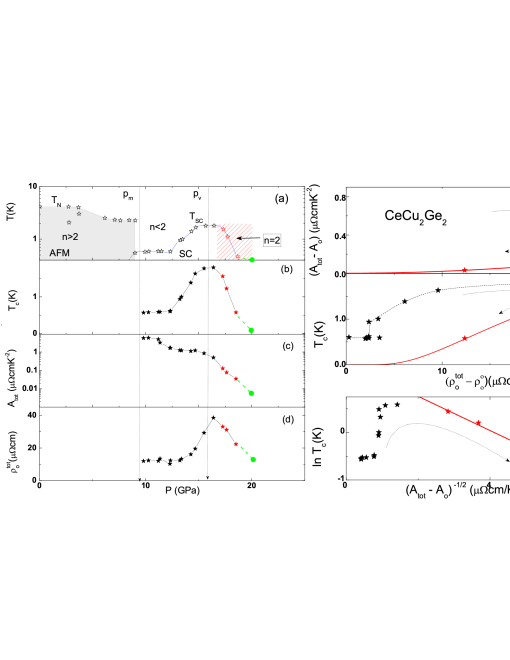
Figure 2: T-p phase diagram and baric evolution of the parameters of CeCu₂Ge₂ (data taken from Ref. ³). (a) A semi-log T-p phase diagram showing the evolution of $T_{N}(p)$, $T_{c}(p)$, and the exponent n(p). Vertical dashed arrows represent $p_{m}\approx 9.4\,$ GPa and $p_{v}\approx 16\,$ GPa.³ The dashed lines are visual guides while the curved arrows signal the direction of pressure increase. The red symbols and hatched area mark the FL region. Evolution of (b) $T_{c}(p)$, (c) $A_{tot}(p)$ in a semi-log plot, and (d) $\rho_{\circ}^{tot}(p)$. As discussed in text, for $p\rightarrow$20 GPa, the pressure-induced strong reduction of the fluctuation leads to $T_{c}\rightarrow T_{c}^{\circ}\approx 0$, $A\rightarrow A_{\circ}$ and $\rho_{\circ}^{tot}\rightarrow\rho_{\circ}^{\circ}$: the limits at 20 GPa (large green circles) are shown in Table LABEL:Tab-Fit-Values-A-Ro-Theta-F. (e) Correlation of $[A_{tot}(p)-A_{\circ}]$ with $[\rho_{\circ}^{tot}-\rho_{\circ}^{\circ}]$. The solid line is a best fit to Eq. 9: $A_{0}$ and $A_{2}$ given in Table LABEL:Tab-Fit-Values-A-Ro-Theta-F. (f) $T_{c}$ versus $[\rho_{\circ}-\rho_{\circ}^{\circ}]$: The solid line is calculated based on Eq. (11) of Subsec. II.3.3. (g) $ln(T_{c})\textit{ versus }(A_{tot}-A_{\circ})^{-\frac{1}{2}}$. The solid red line is the best fit to linearized Eq. 10; $\theta$ and $\mathcal{F}$ parameters are given in Table LABEL:Tab-Fit-Values-A-Ro-Theta-F.

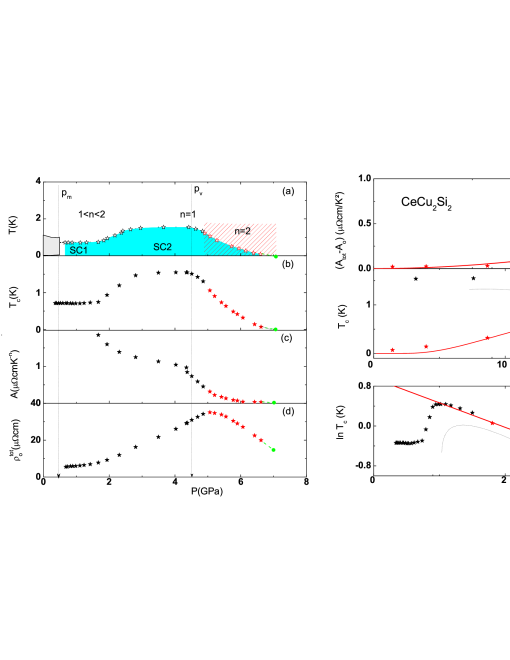
Figure 3: (a) The T-p phase diagram and baric evolution of (b) $T_{c}(p)$, (c) $A_{tot}(p)$, and (d) $\rho_{\circ}^{tot}(p)$ of CeCu₂Si₂. All curves were taken from the continuous line (the visual guide) of Ref. ⁸. For a discussion on the critical pressures $p_{m}$ and $p_{v}$ and the related superconductivity regions (SC 1 and SC II) see Ref. ⁸. The red symbols and hatched area mark the FL region while the dashed lines are visual guides. It is noted that, due to non-stoichiometry, defects, impurities or disorder, the reported parameters of CeCu₂Si₂ vary considerably from sample to sample; nonetheless, the overall evolution as well as the derived correlations are consistently similar.^{23; 24; 25; 26} As $p\rightarrow 7$ GPa, $T_{c}\rightarrow 0$, $A\rightarrow A_{\circ}$ and $\rho_{\circ}\rightarrow\rho_{\circ}^{\circ}$ (see text): the extrapolation to 7 GPa (large green circles) are shown in Table LABEL:Tab-Fit-Values-A-Ro-Theta-F. (e) A plot of [$A(p)-A_{\circ}$] versus [$\rho_{\circ}(p)-\rho_{\circ}^{\circ}$]. The best fit to Eq. 9 is shown as solid red curve; the fit parameters $A_{0}$ and $A_{2}$ are given in Table LABEL:Tab-Fit-Values-A-Ro-Theta-F. (f) $T_{c}$ versus [$\rho_{\circ}(p)-\rho_{\circ}^{\circ}$]: For the solid calculated line, see Eq. (11) in Subsec. II.3.3. (g) $ln(T_{c})$ versus $(A-A_{\circ})^{-\frac{1}{2}}$. The straight red line is a best fit to linearization of Eq. (10): $\theta$ and $\mathcal{F}$ are given in Table LABEL:Tab-Fit-Values-A-Ro-Theta-F.

Table 1: Representative fit parameters of CeCu₂Ge₂, CeCu₂Si₂ and CeCoIn₅. Values of A_o and A₂ were obtained from a fit of Eq. 9 to Figs. 2(e),3(e),4(e)): As $A_{1}\approx 0$, it was fixed as $A_{1}\equiv 0$. For all compounds, $A_{2}$, $\theta$ and $\mathcal{F}$ are close to each other, except $A_{2}$ of CeCoIn5 which is orders of magnitude higher than the others: this together with the high value of $T_{c}$ is most probably related to a relatively high strength of the fluctuation-related e-e scattering channel of CeCoIn5. It is worth noting that the strength and evolution of the fit parameters depend critically on the criteria for determining T_c (10-90%, 50%, onset, zero point etc.) and $A$ (the sample geometry, which is often not precisely determined). Additionally, the widely different methods for sample synthesis and thermal treatment adopted by different groups give rise to a corresponding variation in sample-dependent properties. Although these non-fluctuation-related material properties are accounted for by $T_{\circ}$, $A_{\circ}$, and $\rho_{\circ}^{\circ}$, it is expected to lead to a wide scatter in the fit parameters. The scatter in the experimental curves leads to a large error value.

$HFs$	$\rho_{\circ}^{\circ}$	Ao	A2	$\theta$	$\mathcal{F}$
-	$\mu\Omega\text{cm}$	$\mu\Omega\text{cm/K}^{2}$	$\times 10^{6}\Omega^{-1}\text{cm}^{-1}/\text{K}^{2}$	K	$\times 10^{-3}(\Omega\text{cm/K}^{2})^{1/2}$
CeCu2Ge2	10(1)	2.9(5)$\times 10^{-3}$	2.0(2)$\times 10^{-4}$	4.4(2)	0.36(1)
CeCu2Si2	18.5(5)	0.010(5)	7.0(5)$\times 10^{-4}$	2.6(1)	0.49(1)
CeCoIn5	0.130(5)	0.082(4)	6.0(2)	3.2(1)	0.18(1)

II.2 Empirical analysis: extraction of correlations among $\rho_{\circ}$, $A$, and T_c

Below, we review the baric evolution of $\rho_{\circ}(p)$, $A(p)$, and $T_{c}(p)$ of three representative HF superconductors for which detailed resistivity curves $\rho_{tot}(T,p)$ (essentials for determining these $\rho_{\circ}$, $A$, and $T_{c}$ parameters) were reported. Special attention will be directed towards identifying the correlations.

II.2.1 CeCu${}_{2}X_{2}$ ($X$=Si, Ge)

The T-p phase diagram and the baric evolution of $T_{c}$, $A_{tot}$, and $\rho_{\circ}^{tot}$ of CeCu2Ge2 are shown in Figs. 2(a)-2(d) (Refs. ³; ²⁷) while those of CeCu2Si2 in Figs. 3(a)-3(d) (Refs. ⁴; ²⁶; ²⁸; ²⁹; ⁸). As evident, these plots highlight the dramatic baric evolution in particular around the critical points.

The phase diagram of each of CeCu2X2 manifests a FL character at sufficiently higher pressure; this is evidenced as a quadratic-in-T resistivity contribution, identified in Figs. 2(a) and 3(a) by the hatched area and the n=2 notation. At 20 GPa for CeCu2Ge2 and 7 GPa for CeCu2Si2, $T_{c}\rightarrow 0$; we identify this as a signal of a pressure-induced quench of the fluctuation-related FL contributions. Based on Eqs. 3, all parameters extrapolate to non-fluctuation-related contributions: $A\rightarrow A_{\circ}$ and $\rho_{\circ}\rightarrow\rho_{\circ}^{\circ}$ (see Figs. 2 and 3 and Table LABEL:Tab-Fit-Values-A-Ro-Theta-F).

Then for the purpose of empirical identification of any possible correlation within the FL region, we plot $[A_{\text{tot}}(p)-A_{\circ}]\,\,\it{versus}\,\,[\rho_{\circ}^{tot}(p)-\rho_{\circ}^{\circ}]$ in Figs. 2(e) and 3(e)], $T_{c}\,\,\it{versus}\,\,[\rho_{\circ}^{tot}(p)-\rho_{\circ}^{\circ}]$ in Figs. 2(f) and 3(f)], and $ln[T_{c}(p)]\,\,\it{versus}\,\,1/\sqrt{A_{\text{tot}}(p)-A_{\circ}}$ in Figs. 2(g) and 3(g).

Figures 2(e) and 3(e) show that within the FL state, well above the critical pressures region, ^{1; 2; 30; 25; 26} one obtains

$$(A-A_{\circ})\approx A_{2}(\rho_{\circ}-\rho_{\circ}^{\circ})^{2},$$ (4)

The $A_{\circ}$ and $A_{2}$ parameter of each CeCu2X2 are given in Table LABEL:Tab-Fit-Values-A-Ro-Theta-F. It is noted that the absence of a linear-in-$\rho_{\circ}$ term rules out any Koshino-Taylor contribution. On the other hand, Figs. 2(g) and 3(g) indicate that

$$\ln(T_{c})\propto(A-A_{\circ})^{-\frac{1}{2}}.$$ (5)

A closer look at Eqs. (4 and 5) suggests that a relation between $T_{c}$ and $(\rho_{\circ}-\rho_{\circ}^{\circ})$ can be derived; indeed the solid red curves in Figs. 2(f) and 3(f) were calculated based on Eq. 11 which is a derived equation (see Subsec. II.3.3).

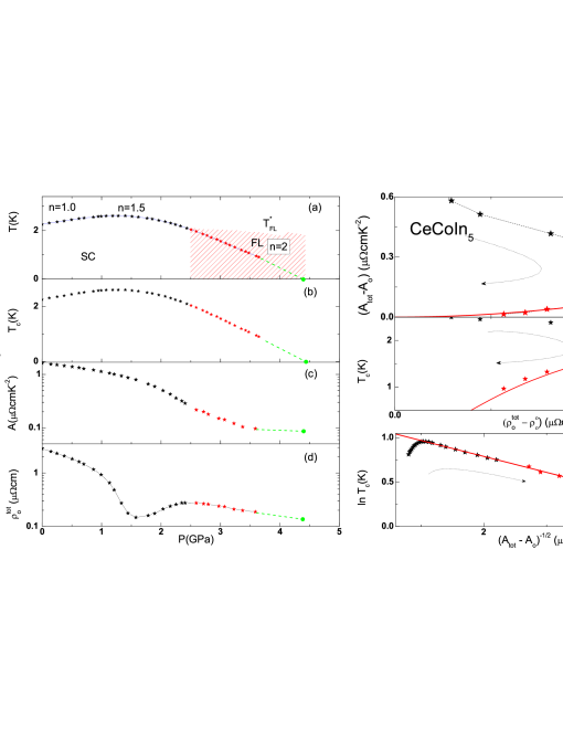
Figure 4: (a) T-p phase diagram and baric evolution of (b) $T_{c}(p)$, (c) $A_{tot}(p)$, and (d) semilog plot of $\rho_{\circ}^{tot}(p)$ of CeCoIn₅. All curves were taken from the continuous line (the visual guide) of Ref. ¹⁶. For more detail on this phase diagram, in particular, the position of critical $p_{m}$, see Refs. ¹⁶; ³¹; ³²; ³³. The red symbols and hatched area identify the FL region while the dashed lines are visual guides. For $p\rightarrow$4.4 GPa, $T_{c}\rightarrow 0$, $A\rightarrow A_{\circ}$ and $\rho_{\circ}\rightarrow\rho_{\circ}^{\circ}$ (see text and Table LABEL:Tab-Fit-Values-A-Ro-Theta-F). (e) A plot of $A_{tot}-A_{\circ}$ versus $\rho_{\circ}^{tot}-\rho_{\circ}^{\circ}$. The solid curve is the best fit to Eq. 9 (see Table LABEL:Tab-Fit-Values-A-Ro-Theta-F). (f) $T_{c}$ versus ($\rho_{\circ}^{tot}-\rho_{\circ}^{\circ}$): The solid calculated line is based on Eq. (11). (g) $ln(T_{c})$ versus $(A-A_{\circ})^{-\frac{1}{2}}$. The best fit to the linearization of Eq. (10) (see Table LABEL:Tab-Fit-Values-A-Ro-Theta-F for the fit parameters).

II.2.2 CeCoIn₅

The T-p phase diagram of CeCoIn₅ [Refs. ¹⁶; ³⁴; ³¹; ³²] is shown in Fig. 4(a) while the baric evolution of $T_{c}(p)$, $A_{tot}(p)$ and $\rho_{\circ}^{tot}(p)$ are shown in Figs. 4(b), 4(c) and 4(d), respectively.

A comparison of the features of CeCoIn₅ with those of CeCu${}_{2}X_{2}$ ($X$=Si, Ge) suggests an overall similarity in that:

• Figure 4(e) indicates that $A(p)-A_{\circ}$ is large but still quadratic-in-$[\rho_{\circ}(p)-\rho_{\circ}^{\circ}$],

• Figure 4(f) reveals that the evolution of $T_{c}[\rho_{\circ}(p)-\rho_{\circ}^{\circ}]$ can be described by Eq. 11 (see Subsec. II.3.3).

• Figure 4(g) shows that $\ln[T_{c}(p)]$ is linear in $[A(p)-A_{\circ}]^{-\frac{1}{2}}$ .

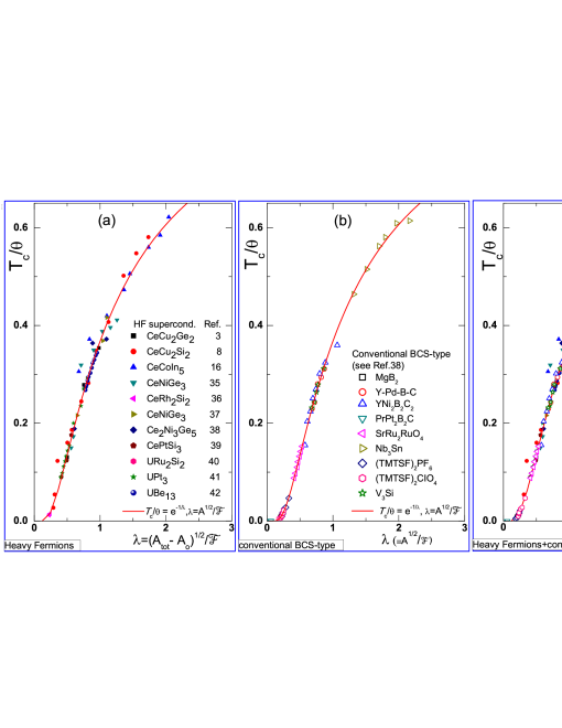
Figure 5: (a) The generalized plot of $\frac{T_{c}(p)}{\theta}$versus $\lambda=\frac{(A-A_{\circ})^{\frac{1}{2}}}{\mathcal{F}}$ of the tabulated HF superconductors. ^{3; 8; 25; 16; 35; 36; 37; 38; 39; 40; 41; 42} (b) For comparison, we include the plot of the same relation in conventional superconductors (data taken from Ref. [⁴³]). (c) A collapse of data from all HF and conventional superconductors on the single $T_{c}/\theta=exp(-1/\lambda)$ curve: an unsurprising result considering panels (b and c); nevertheless, considering the diversity of the superconducting materials, this plot is highly nontrivial. Each pair of sample-dependent $\theta$ and $\mathcal{F}$ was evaluated within the pressure range wherein Eq. (10) is valid [see Figs. 2(g), 3(g), and 4(g)]. Representative values of $\theta$ and $\mathcal{F}$ are shown in Table LABEL:Tab-Fit-Values-A-Ro-Theta-F. As evident, the distribution region of the pairs ($T_{c}/\theta$, $\lambda$) in both HF and strong-coupled superconductors are similar, with the upper limit being $\approx(0.6,2.1)$ (for $\lambda$ limit of strong superconductors, see Ref. ²⁰ and also Fig. 4 of Ref. ⁴³). As mentioned for CeCu2X2 and CeCoIn5, $\lambda$ is corrected using $\frac{(A-A_{\circ})^{\frac{1}{2}}}{\mathcal{F}}$. Similar plot, but with no $\frac{(A-A_{\circ})^{\frac{1}{2}}}{\mathcal{F}}$ correction, was reported for both pnictide and chalcognides superconductors.^{44; 45} Finally, it is emphasized that the relatively high values of $\frac{T_{c}(p)}{\theta}$ (those close to 1) should not be substituted in Eq. 14 since this equation is valid only within the $\frac{T_{c}}{\theta}\ll 1$ condition.⁴⁶

II.3 Theoretical analysis: interpretation of the correlations among $\rho_{\circ}$, $A$, and T_c

The aforementioned experimental evidences emphasize that in spite of the wide differences in material properties of these HF superconductors, one observes: (i) A similarity in the overall evolution of the phase diagrams as well as in the baric evolution of their $T_{c}(p)$, $A(p)$, and $\rho_{\circ}(p)$. (ii) A nontrivial manifestation of neighboring superconductivity and FL phases. (iii) Two correlations (expressed in Eqs. 4 and 5) and a derived one; all manifested in Figs. 2,3,4. Below we discuss the significance of these features in terms of a fluctuation-mediated e-e scattering channel which, due to a modification in the kinematic constraints, is endowed with a significantly enlarged phase space for scattering, much larger than the traditional Baber or Umklapp e-e scattering channels.⁴⁷

Furthermore, the empirical analysis highlights the distinct and nontrivial contrast between the properties of the FL state of a HF superconductor and that of conventional weakly-correlated superconductor: It is remarkable that $A$ is more than five orders of magnitude higher than the contribution expected for a typical Fermi-liquid metal ($A_{\circ}\simeq 10^{-7}\mu\Omega$cm/K²).^{48; 49; 50; 51; 52; 53}

Another contrast is that a conventional FL superconductor, in contrast to a HF one, does not manifest a correlation among $\rho_{\circ}$, $T_{c}$ and $A$: $\rho_{\circ}$ is determined by the electron-impurity scattering, $\rho_{\circ}\sim|V_{imp}|^{2}$; $T_{c}\sim e^{-1/\lambda}$ is associated with electron-phonon coupling, $\lambda\sim|V_{ep}|^{2}$; while $A$ depends on e-e interaction, $A\sim|V_{ee}|^{2}$.

It is worth emphasizing that, although two exceptional cases were reported to yield a similar BCS-like correlation among $T_{c}$ and $A$ (see Ref. ⁵⁴ and Subsec. II.2), none of them manifest a correlation between $A$ and $\rho_{\circ}$ nor between $T_{c}$ and $\rho_{\circ}$; in fact, Anderson theorem excludes the latter relation. It is, then, quite puzzling that the aforementioned empirical analysis, see Figs. 2-4, delineate a distinct FL phase within which one identifies a surge of superconductivity and pressure-dependent correlations among $\rho_{\circ}$, $A$ and $T_{c}$. This puzzle can be resolved if the manifestation of superconductivity and FL state as well as the correlation of $T_{c}$ (hallmark of superconductivity) and $A$ (hallmark of normal FL state) are assumed to be driven by a retarded, spin-fluctuation ⁶ or valence-fluctuation ⁷ mediated e-e interaction. This is reminiscent of the defect-induced, phonon-mediated e-e scattering in defectal-bearing systems (see Ref. ⁴⁷)

The basic idea is discussed in Subsect.II.1: within a HF superconducting sample, the fluctuation-related quasiparticles can be created or annihilated and that their mediation of the e-e interaction, $V^{f}_{ee}$,^{6; 7} is the driving mechanism behind the surge of each of these features. We illustrate this argument by considering the spin-fluctuation case, as in Ref. ⁶. There, $I^{2}\chi(\omega)$ [$I$ is an exchange coupling while $\chi(\omega)$ is a dynamic susceptibility] plays the same role as that of Eliashberg’s electron-phonon spectral function $\alpha^{2}\mathcal{F}\left(\omega\right)$. $V^{sf}_{ee}$ can then be obtained from the integral over frequencies of such an Eliashberg’s type spectral function.

Below, we give a short summary of the main expressions describing $T_{c}(\ell)$, $A(\ell)$ and their correlations with each other as well as with $\rho_{\circ}(\ell)$.

II.3.1 Expression of $T_{c}(\ell)$

Adopting the traditional strategy for calculating $T_{c}(\ell)$, we solved the set of coupled linearized Eliashberg’s equations within the BCS limit. In this limit, $T_{c}(\ell)$ is determined by the superconducting coupling constant $\lambda(\ell)=N(\epsilon_{F})V_{ee}^{sf}(\ell)=2\int d\omega\frac{I^{2}\chi(\omega)}{\omega_{opt}^{2}+\omega^{2}}$, where $\omega_{opt}$ is an optimal frequency at which $\lambda$ is maximal, and can thus be written as: ⁴⁷

$$T_{c}(\ell)=\theta\,exp\Bigg{(}{\frac{-1-\lambda(\ell)}{\lambda(\ell)-\mu^{*}}}\Bigg{)},$$ (6)

where $\mu^{*}$ is the Coulomb pseudopotential and $\theta$ is an energy scale that depends on the cut-off bandwidth $\omega_{c}^{sf}$.

II.3.2 Expression of $A(\ell)$

Applying a variational approach to the linearized version of Boltzmann’s transport equations within the relaxation time approximation (wherein the inverse scattering time is calculated by the use of Fermi’s golden rule) we obtain⁴⁷ $\rho(\ell)=A(\ell)T^{2}$ and

$$A(\ell)=F^{2}_{\ell}\left|\frac{\lambda(\ell)-\mu^{*}}{1+\lambda(\ell)}\right|^{2}.$$ (7)

Here, $F_{\ell}$ represents the efficiency of momentum relaxation and the availability of phase space for scattering.⁴⁷ Within the FL phase, $\ell$ is long, $1\ll k_{F}\ell_{p}<\infty$, and $\rho_{\circ}$ is small ($k_{F}$ = Fermi wave number); as such, Eq. (7) can be expanded around $\lambda_{\circ}=\lambda(\ell\rightarrow\infty)$ of the normal matrix as

$$A(\ell)\simeq a_{\circ}+a_{1}(\delta\lambda)+a_{2}(\delta\lambda)^{2}+\mathcal{O}[(\delta\lambda)^{3}],$$ (8)

wherein $a_{\circ}=A(\ell\rightarrow\infty)=\frac{|\lambda_{\circ}-\mu^{*}|^{2}}{1+\lambda_{\circ}}$ refer to the negligibly small kinematically-constrained non-fluctuating contributions; the second and third term [containing $\delta\lambda=\lambda(\ell)-\lambda_{\circ}$ and the coefficients $a_{1}=2F^{2}_{\ell}(|\lambda_{\circ}-\mu^{*}|(1+\mu^{*}))/(1+\lambda_{\circ})^{3}$ and $a_{2}=F^{2}_{\ell}(1+\mu^{*}-2|\lambda_{\circ}-\mu^{*}|)(1+\mu^{*})/(1+\lambda_{\circ})^{4}$] denote contributions from all kinematically unconstrained relaxation processes after incorporating the fluctuation-mediated channel.

The second-order polynomial expression of $A(\ell)$, Eq. 8, is reminiscent of the empirical quadratic-in-$\rho_{\circ}$ of Eq. 4. Below we look for an analytical description of $A(\rho_{\circ})$. Let us start by recalling that, in a typical Fermi liquid, the frequency dependence of the imaginary part of the self energy is given by ${\cal I}m\Sigma(\omega)\sim\omega^{2}$. Then, on considering the relevant energy scale to be set by $k_{B}T$, one obtains the characteristic FL quadratic-in-T resistivity. Intuitively, this is related to the fact that, for a given temperature $T$, $N(E_{F})k_{B}T$ single particles within the Fermi surface are participating in the fluctuation-mediated two-particle channel (each single particle can scatter into one another via this fluctuation-mediated scattering process): this generates the well-known $AT^{2}$ resistivity contribution. Specifically, our analysis showed that this channel leads to a FL state with $A$ as in Eq. 7 and superconductivity with $T_{c}$ as in Eq. 6. Moreover, at $T=0$ limit, the relevant energy scale is set by the fuzziness of the Fermi surface which is determined by $\delta g$. Just as the case for the $\omega^{2}$-leading-to-$T^{2}$-contribution, we expect $\rho_{\circ}\propto\delta\lambda\propto(\delta g)^{2}$.⁵⁵ This allows us to establish a correlation among $\rho_{\circ}$ and each of $T_{c}$ and $A$ (each is a function of $\ell$). Guided by these considerations, as well as the empirical relation of Eq. 4, we consider

$$A(\ell)\simeq A_{\circ}+A_{1}(\rho_{\circ})+A_{2}(\rho_{\circ})^{2},$$ (9)

where $A_{i}(i=0,1,2$) are functions of $F^{2}_{\ell},~{}\mu^{*},\text{ and }\lambda_{\circ}$. Eq. 9 suggests three limiting contributions to $A(\ell)$: (i) The host contribution (dominant $A_{\circ}\neq 0$ when $A_{1}\approx 0$ and $A_{2}\approx 0$); (ii) a single-particle-like Koshino-Taylor-type $(A-A_{\circ})\propto\rho_{\circ}$, contribution (dominant $A_{1}\neq 0$ contribution); and (iii) an $(A-A_{\circ})\propto(\rho_{\circ})^{2}$ contribution (a dominant $A_{2}$ and a negligible $A_{1}$). Results of Figs. 2(e), 3(e), 4(e) belong to the third case.

II.3.3 Correlation between $T_{c}(\ell)$ and $A(\ell)$

Combining the expressions for $T_{c}(\ell)$ in Eq. 6 and $A(\ell)$ in Eq. 7, we arrive at:

$$T_{c}(\ell)=\theta\,e^{-\mathcal{F}/\sqrt{A(\ell)}}.$$ (10)

This universal and exact kinematic scaling relation (valid for long $\ell$, low $\rho_{\circ}$: the Fermi-liquid region) is the essence of the relations of Eq. (5) and Figs. 2(g), 3(g), and 4(g). Eq. (10) is most remarkably manifested in Fig. 5: an increase (decrease) of pressure leads to a downwards (upwards) flow of $T_{c}(\ell)$ towards weaker (stronger) couplings, without ever leaving the curve given by Eq.  (10).

Finally, a simplified but approximate relation between $T_{c}$ and $(\rho_{\circ}-\rho_{\circ}^{\circ})$ can be obtained in the specific case wherein the quadratic-in-$\rho_{\circ}$ term in Eq. 9 is dominant. Substituting Eqs. (4 and 7) into Eq. 10, we obtain

$$T_{c}(\ell)\approx\theta\,exp\big{(}\frac{-\mathcal{F}}{\sqrt{A_{2}}\big{[}\rho_{\circ}(\ell)-\rho_{\circ}^{\circ}\big{]}}\big{.}$$ (11)

On substituting $\theta$, $\mathcal{F}$, $A_{2}$, and $\rho_{\circ}^{\circ}$ of Table LABEL:Tab-Fit-Values-A-Ro-Theta-F into this equation, one obtains the solid curves of Figs. 2(f), 3(f), 4(f); this excellent description of experimental data with no fitting parameters is no surprise since, as mentioned above, Eq. (11) is a derived one.

III Discussion and Conclusions

The similarity of the phase diagrams shown in Figs. 2,3,4, as well as those of other HF superconductors,^{1; 2} suggests a generalized T-p phase diagram that highlights the similarity in the cascade of distinct electronic states and in the overall evolution of $T_{c}(\ell)$, $A(\ell)$, and $\rho_{\circ}(\ell)$. Of particular interest to this work is the nontrivial manifestation, in all phase diagrams, of a superconductivity, a FL character and their correlations (see Figs. 2, 3, 4, and 5). We argue above that the surge of all these features and correlations is driven by the spin-fluctuation/valence-fluctuation mediated e-e channel operating within the FL range of the studied HF superconductors.⁵⁶

It happened that for these fluctuations to be well defined quasiparticles and for the Migdal-Eliashberg theoretical framework to be applicable, one needs to ensure that $\ell$ is long which for the spin-fluctuation case translates into $\chi(\omega)$ and $V^{sf}_{ee}$ being weak and, as a consequence, reduced $\rho_{\circ}$, $A$, and T_c. In fact this argument, turned around, can be used to define the FL range which can be reached by an application of higher pressure (see Figs. 2- 4), strong magnetic field,^{31; 32; 33} or incorporation of nonmagnetic impurities: ^{57; 58; 59; 60} All promote the weakening of the fluctuation-mediated scattering process.

Based on these arguments, the following inferences can be drawn: First, Figs. 2- 4 indicate that on moving out of the FL region but towards the quantum critical points, one observes a continuous enhancement in $\rho_{\circ}$, $A$, and $T_{c}$. This continuity is suggestive of a similarity in the scattering interaction, the strength of which is enhanced on reducing the pressure. However, Figs. 2-4 also indicate that below the FL region our analytical expressions do not reproduce the observed baric evolution of $A$ or $T_{c}$. This shortcoming is related to the breakdown of the long-$\ell$ condition. Nevertheless, this does not invalidate our analysis within the FL region. It is worth repeating that the availability of a FL state is not a precondition for the applicability of our approach. Rather, the surge of the e-e scattering channel gives rise to the FL state, the superconductivity and their correlation.

Second, it was reported that an application of a magnetic field ($H>H_{2}$) within the superconducting dome of CeCoIn₅ leads to a quench of superconductivity in favor of a FL normal-state.^{31; 32; 33} We attribute this field-induced FL character within the NFL region to a field-induced weakening of the strength of the spin-fluctuation and as such to an increase in $\ell$, in reminiscence of the aforementioned increase in applied pressure or in the incorporation of nonmagnetic impurities. Further analysis is underway.

Third, we argued above that within the long-$\ell$ region, the spin-fluctuation/valence-fluctuation modes are mediating the e-e interaction and this in turn leads to the scaling between $\frac{T_{c}}{\theta}$ and $(A_{tot}-A_{\circ})$ (see Fig. 5(a)). This is similar to the emergent phonon-mediated scaling reported for other non-HF superconductors: Fig. 5(b) demonstrates the scaling in conventional superconductors.^{47; 43} Similar scaling was reported for the Fe-based pnictides⁴⁴ and chalcogenides:⁴⁵ Although the superconductivity in these series are considered to be driven by spin-fluctuation mediated pairing¹⁰ however we did not include these Fe-based materials in Fig.5 since these reports did not include a correction for the non-fluctuation-related contribution: $A_{tot}$ was used instead of $(A_{tot}-A_{\circ})$.

We extend our present analysis by including a discussion⁴⁷ of two specific parameters of the HF superconductors: (i) the Kadowaki-Woods ratio and (ii) the gap-to-$T_{c}$ ratio. We show that the influence of the fluctuation processes on both ratios can be accounted for by including an additional factor which embodies the material properties of these HF superconductors.

(i) Jacko et al.⁶¹ accounted for the wide difference among the Kadowaki-Woods ratio of a variety of strongly coupled systems by demonstrating that

$$\frac{A}{\gamma^{2}}=\Big{(}\frac{81}{4\pi\hbar k_{B}^{2}e^{2}}\Big{)}\Big{(}\frac{1}{d^{2}nN^{2}(\epsilon_{F})\langle v_{0x}^{2}\rangle}\Big{)}=\Big{(}f_{con}\Big{)}\Big{(}\frac{1}{f_{mat}}\Big{)},$$ (12)

wherein $\langle v_{0x}^{2}\rangle$ is an average of the carrier velocity squared (a measure of the anisotropies), $n$ is the carrier density, $N(\epsilon_{F})$ is the density of states at the Fermi level, and $d\sim 1$ is a dimensionless number. Apparently, due to the material-dependent second factor, $\frac{A}{\gamma^{2}}$ of Eq. 12 is nonuniversal. This shortcoming would be most evident for the ratio of the fluctuation-bearing HF superconductors within their Fermi-liquid region (see Figs. 2-4). Our evaluation of the Kadowaki-Woods ratio (Eq. 12) of these HF superconductors gives

$$\frac{A}{\gamma^{2}}=\Big{(}\frac{81}{4\pi\hbar k_{B}^{2}e^{2}}\Big{)}\Big{(}\frac{F_{\ell}}{d^{2}nN^{2}(\epsilon_{F})\langle v_{0x}^{2}\rangle}\Big{)}=\Big{(}f_{con}\Big{)}\Big{(}\frac{F_{\ell}}{f_{mat}}\Big{)},$$ (13)

wherein the material-dependent $F_{\ell}$ factor is as described in Eq. (7). It is not close to 1 as assumed during the derivation of Eq. (12).⁶¹ Rather $F_{\ell}>1$: a larger apparent ratio because of the easing of the kinematic constraints in these fluctuation-bearing systems. As in Ref. ⁶¹, the universal character is restored only when expressed as $\frac{A}{\gamma^{2}}\Big{(}\frac{f_{mat}}{F_{\ell}}\Big{)}=\frac{A.f_{mat}^{{}^{\prime}}}{\gamma^{2}}=f_{con}$.

(ii) Carbotte⁴⁶ derived an approximate expression for the gap-to-$T_{c}$ ratio of strong-coupled superconductor. Modified to the case of a fluctuation-bearing superconductor within $\frac{T_{c}}{\theta}\ll 1$ region, this expression reads as

$$\frac{2\Delta(\ell)}{k_{B}T_{c}(\ell)}\approx 3.53\left\{1+12.5\left[\frac{T_{c}(\ell)}{\theta}\right]^{2}\ln{\left[\frac{\theta}{2T_{c}(\ell)}\right]}\right\},$$ (14a)

$$\approx 3.53\left\{1+12.5\left[e^{-\mathcal{F}/\sqrt{A(\ell)}}\right]^{2}\ln{\left[\frac{1}{2e^{-\mathcal{F}/\sqrt{A(\ell)}}}\right]}\right\}$$ (14b)

Thus, within $\frac{T_{c}}{\theta}\ll 1$ region, the gap-to-$T_{c}$ ratio can be fine-tuned: From $2\Delta(\ell\rightarrow\infty)/k_{B}T_{c}(\ell\rightarrow\infty)=3.53$, the universal BCS value, up to a higher nonuniversal value by varying the control-parameter that modifies $\ell$.

Finally, it is worth adding that our internally-consistent empirical and theoretical analyses are based on a clear identification of the difference between the fluctuation-related and normal (non-fluctuation-related) contributions within the fluctuation-related FL region (which starts when the resistivity manifests the $T^{2}$ contribution and ends when $T_{c}\rightarrow 0$).

In summary, we investigated the superconductivity, the FL transport, and their correlations within the FL region of the T-p phase diagram of representative quantum-critical HF superconductors. Empirically, on varying the control parameters, (i) the normal-state resistivities manifest the characteristic FL, $\rho_{o}+\textit{AT}^{2}$, character with $A\propto\rho_{\circ}^{2}$ and (ii) the superconducting state manifests a correlation of $T_{c}$ with $A$ ($ln\frac{T_{c}}{\theta}\propto A^{-\frac{1}{2}}$). We attribute the surge of these superconducting and FL transport features and their correlations to a fluctuation-mediated e-e scattering channel. Theoretically, on adopting many-body techniques, we derive analytic expressions for $T_{c}(\rho_{\circ})$ and $A(\rho_{\circ})$ and their correlations that reproduce satisfactorily the aforementioned empirical correlations.

Methods

We analyzed the extensively reported pressure-dependent resistivities of various HF superconductors. Within the FL region, we looked for any correlation among the superconductivity (as measured by $T_{c}$), the Fermi-liquid character (as measured by $A$), and the excess in the residual resistivity ($\rho_{\circ}$ as a measure of the strength of the scattering channel) when the control parameter is varied. Using graphical and analytical procedures, we managed to identify the empirical expression discussed in Subsec. II.2. More importantly, we managed to identify the spin-fluctuation/valence-fluctuation mediated e-e scattering channel as being the driving mechanism behind these correlations. Guided by the inferences drawn from the empirical expressions and the identified channel, we formulated the theoretical framework outlined in Subsec. II.2 and Sec. II.3: Basically, we started with the spin-fluctuation/valence-fluctuation exchange mechanism which is different from the traditional mechanisms in that it takes into consideration the modification in the kinematic constraints which, in turn, lead to a significant enlargement in the phase space available for scattering. Then, after applying the standard theories of Migdal-Eliashberg (superconductivity) and Boltzmann (transport), we managed to derive the analytic expressions of Subsec. II.2 which satisfactorily explain the empirical observations.

References

- Gegenwart et al. (2008) P. Gegenwart, Q. Si, and F. Steglich, Nat. Phys. 4, 186 (2008).
- Coleman (2007) P. Coleman, Handbook of Magnetism and Advanced Magnetic Materials (2007).
- Jaccard et al. (1999) D. Jaccard, H. Wilhelm, K. Alami-Yadri, and E. Vargoz, Physica B 259-261, 1 (1999).
- Yuan et al. (2003) H. Q. Yuan, F. M. Grosche, M. Deppe, C. Geibel, G. Sparn, and F. Steglich, Science 302, 2104 (2003).
- Löhneysen et al. (2007) H. v. Löhneysen, A. Rosch, M. Vojta, and P. Wölfle, Rev. Mod. Phys. 79, 1015 (2007).
- Mathur et al. (1998) N. D. Mathur, F. M. Grosche, S. R. Julian, I. R. Walker, D. M. Freye, R. K. W. Haselwimmer, and G. G. Lonzarich, Nature 394, 39 (1998).
- Miyake and Watanabe (2017) K. Miyake and S. Watanabe, Philos. Mag. 97, 3495 (2017).
- Holmes et al. (2004) A. T. Holmes, D. Jaccard, and K. Miyake, Phys. Rev. B 69, 024508 (2004).
- Pines (2013) D. Pines, J. Phys. Chem. B 117, 13145 (2013).
- Scalapino (2012) D. J. Scalapino, Reviews of Modern Physics 84, 1383 (2012).
- Maier et al. (2020) T. A. Maier, S. Karakuzu, and D. J. Scalapino, Phys. Rev. Research 2, 033132 (2020).
- Li et al. (2021) Z. Li, S. Kivelson, and D. Lee, npj Quantum Mater 6, 36 (2021).
- Dean et al. (2013) M. Dean, G. Dellea, R. S. Springell, F. Yakhou-Harris, K. Kummer, N. Brookes, X. Liu, Y. Sun, J. Strle, T. Schmitt, et al., Nature materials 12, 1019 (2013).
- Lee-Hone et al. (2020) N. Lee-Hone, H. Özdemir, V. Mishra, D. Broun, and P. Hirschfeld, Phys. Rev. Res. 2, 013228 (2020).
- Lee-Hone et al. (2017) N. Lee-Hone, J. Dodge, and D. Broun, Phys. Rev, B 96, 024501 (2017).
- Sidorov et al. (2002) V. Sidorov, M. Nicklas, P. Pagliuso, J. Sarrao, Y. Bang, A. V. Balatsky, and J. D. Thompson, Phys. Rev. Lett. 89, 157004 (2002).
- (17) The assumption of a formation of a patch within which quantum critical fluctuations emerge does not contradict the requirement that quantum critical fluctuations are scale invariant and extend over a large-sized region.This is because the length scale of each patch is taken to be longer than the mean free path and coherence length. This assumption is is invoked for taking care of the excess residual resistivity and its usefulness in reconciling the influence from each of disorder, pressure or magnetic field. Within each patch, .
- Bergmann (1971) G. Bergmann, Phys. Rev. B 3, 3797 (1971).
- Bergmann (1976) G. Bergmann, Phys. Rep. 27, 159 (1976).
- Gurvitch (1986) M. Gurvitch, Phys. Rev. Lett. 56, 647 (1986).
- (21) In cases where , one considers .
- (22) An incorporation of nonmagnetic impurities 57; 58; 59; 60 leads to a reduction in and and, as a consequence, to a drop in both A and Tc.
- Rosch (1999) A. Rosch, Phys. Rev. Lett. 82, 4280 (1999).
- Kambe and Flouquet (1997) S. Kambe and J. Flouquet, Solid State Commun. 103, 551 (1997).
- Sheikin et al. (2000) I. Sheikin, D. Braithwaite, J.-P. Brison, W. Assmus, and J. Flouquet, J. Low Temp. Phys. 118, 113 (2000).
- Gegenwart et al. (1998) P. Gegenwart, C. Langhammer, C. Geibel, R. Helfrich, M. Lang, G. Sparn, F. Steglich, R. Horn, L. Donnevert, A. Link, and W. Assmus, Phys. Rev. Lett. 81, 1501 (1998).
- Honda et al. (2013) F. Honda, T. Maeta, Y. Hirose, Y. Ōnuki, A. Miyake, and R. Settai, J. Korean Phys. Soc. 63, 345 (2013).
- Bellarbi et al. (1984) B. Bellarbi, A. Benoit, D. Jaccard, J. M. Mignot, and H. F. Braun, Phys. Rev. B 30, 1182 (1984).
- Rueff et al. (2011) J.-P. Rueff, S. Raymond, M. Taguchi, M. Sikora, J.-P. Itié, F. Baudelet, D. Braithwaite, G. Knebel, and D. Jaccard, Phys. Rev. Lett. 106, 186405 (2011).
- Miranda and Dobrosavljević (2005) E. Miranda and V. Dobrosavljević, Rep. on Prog. in Phys. 68, 2337 (2005).
- Paglione et al. (2003) J. Paglione, M. A. Tanatar, D. G. Hawthorn, E. Boaknin, R. W. Hill, F. Ronning, M. Sutherland, L. Taillefer, C. Petrovic, and P. C. Canfield, Phys. Rev. Lett. 91, 246405 (2003).
- Bianchi et al. (2003) A. Bianchi, R. Movshovich, I. Vekhter, P. G. Pagliuso, and J. L. Sarrao, Phys. Rev. Lett. 91, 257001 (2003).
- Bauer et al. (2005) E. D. Bauer, C. Capan, F. Ronning, R. Movshovich, J. D. Thompson, and J. L. Sarrao, Phys. Rev. Lett. 94, 047001 (2005).
- Ronning et al. (2006) F. Ronning, C. Capan, E. D. Bauer, J. D. Thompson, J. L. Sarrao, and R. Movshovich, Phys. Rev. B 73, 064519 (2006).
- Kotegawa et al. (2006) H. Kotegawa, K. Takeda, T. Miyoshi, S. Fukushima, H. Hidaka, T. C. Kobayashi, T. Akazawa, Y. Ohishi, M. Nakashima, A. Thamizhavel, et al., J. Phys. Soc. Jpn. 75, 044713 (2006).
- Araki et al. (2002) S. Araki, M. Nakashima, R. Settai, T. C. Kobayashi, and Y. Onuki, J. Phys.: Condens. Matter 14, L377 (2002).
- Nakashima et al. (2004) M. Nakashima, K. Tabata, A. Thamizhavel, T. C. Kobayashi, M. Hedo, Y. Uwatoko, K. Shimizu, R. Settai, and Y. Onuki, J. Phys.: Condens. Matter 16, L255 (2004).
- Nakashima et al. (2006) M. Nakashima, H. Kohara, A. Thamizhavel, T. D. Matsuda, Y. Haga, M. Hedo, Y. Uwatoko, R. Settai, and Y. Ōnuki, Physica B: Cond Matter 378, 402 (2006).
- Onuki et al. (2008) Y. Onuki, Y. Miyauchi, M. Tsujino, Y. Ida, R. Settai, T. Takeuchi, N. Tateiwa, T. D. Matsuda, Y. Haga, and H. Harima, J. Phys. Soc. Jpn. 77, 37 (2008).
- Hassinger et al. (2008) E. Hassinger, G. Knebel, K. Izawa, P. Lejay, B. Salce, and J. Flouquet, Phys. Rev. B 77, 115117 (2008).
- de Visser et al. (1984) A. de Visser, J. Franse, and A. Menovsky, J. Magn. Magn. Mater. 43, 43 (1984).
- Ott et al. (1983) H. R. Ott, H. Rudigier, Z. Fisk, and J. L. Smith, Phys. Rev. Lett. 50, 1595 (1983).
- Nunez-Regueiro et al. (2012) M. Nunez-Regueiro, G. Garbarino, and M. D. Nunez-Regueiro, J Phys: Conf. Series 400, 022085 (2012).
- Castro et al. (2018) P. B. Castro, J. L. Ferreira, M. B. S. Neto, and M. ElMassalami, J. Phys.: Conf. Ser. 969, 012050 (2018).
- Soares et al. (2018) C. Soares, M. ElMassalami, Y. Yanagisawa, M. Tanaka, H. Takeya, and Y. Takano, Sci. Rep. 8, 7041 (2018).
- Carbotte (1990) J. P. Carbotte, Rev. Mod. Phys. 62, 1027 (1990).
- ElMassalami and Neto (2021) M. ElMassalami and M. B. S. Neto, Phys. Rev. B 104, 014520 (2021).
- Lawrence and Wilkins (1973) W. E. Lawrence and J. W. Wilkins, Phys. Rev. B 7, 2317 (1973).
- Lawrence (1976) W. E. Lawrence, Phys. Rev. B 13, 5316 (1976).
- MacDonald (1980) A. H. MacDonald, Phys. Rev. Lett. 44, 489 (1980).
- MacDonald et al. (1981) A. H. MacDonald, R. Taylor, and D. J. W. Geldart, Phys. Rev. B 23, 2718 (1981).
- Patton and Zaringhalam (1975) B. Patton and A. Zaringhalam, Phys. Lett. A 55, 95 (1975).
- Pethick et al. (1986) C. J. Pethick, D. Pines, K. F. Quader, K. S. Bedell, and G. E. Brown, Phys. Rev. Lett. 57, 1955 (1986).
- not (a) (a), see Ref. 47 for a discussion on the two reported exceptions.
- not (b) (b), based on Eq. (5) of Ref. 62, for low defects, one obtains .
- not (c) (c), such an argument, supported by the aforementioned agreement between theory and experiments, is not in contradiction with the fact that there are difference in the details of the corresponding phase diagrams (e.g. the number and type of -domes, the number and type of the critical/crossover points , , etc.): In fact, irrespective of these details, all studied phase diagrams manifest quantum critical instabilities which are accompanied by critical spin-fluctuations6 or valence-fluctuations8; 7.
- Smith et al. (1984) J. L. Smith, Z. Fisk, J. O. Willis, B. Batlogg, and H. R. Ott, J Appl Phys 55, 1996 (1984).
- Adrian and Saemann-Ischenko (1988) G. Adrian and G. Saemann-Ischenko, Zeitschrift für Physik B Condensed Matter 72, 235 (1988).
- Adrian and Adrian (1988) G. Adrian and H. Adrian, Physica C: Superconductivity 153-155, 435 (1988).
- Adrian and Adrian (1989) G. Adrian and H. Adrian, J Less Common Met 149, 313 (1989).
- Jacko et al. (2009) A. C. Jacko, J. O. Fjærestad, and B. J. Powell, Nat Phys 5, 422 (2009).
- Bergmann (1969) G. Bergmann, Z. Physik 228, 25 (1969).