A robust and efficient line search for self-consistent field iterations

Abstract

We propose a novel adaptive damping algorithm for the self-consistent field (SCF) iterations of Kohn-Sham density-functional theory, using a backtracking line search to automatically adjust the damping in each SCF step. This line search is based on a theoretically sound, accurate and inexpensive model for the energy as a function of the damping parameter. In contrast to usual SCF schemes, the resulting algorithm is fully automatic and does not require the user to select a damping. We successfully apply it to a wide range of challenging systems, including elongated supercells, surfaces and transition-metal alloys.

I Introduction

Ab initio simulation methods are standard practice for predicting the chemical and physical properties of molecules and materials. At the level of simulating electronic structure the majority of approaches are either directly based upon Kohn-Sham density-functional theory (DFT) or Hartree-Fock (HF) or use these techniques as starting points for more accurate post-DFT or post-HF developments. Both HF and DFT ground states are commonly found by solving the self-consistent field (SCF) equations, which for both type of methods are very similar in structure. Being thus fundamental to electronic-structure simulations substantial effort has been devoted in the past to develop efficient and widely applicable SCF algorithms. We refer to Woods et al. (2019) and Lehtola et al. (2020) for recent reviews on this subject.

However, the advent of both cheap computational power as well as the introduction of data-driven approaches to materials modelling has caused simulation practice to change noticeably. In particular in domains such as catalysis or battery research where experiments are expensive or time-consuming, it is now standard practice to perform systematic computations on thousands to millions of compounds. The aim of such high-throughput calculations is to either (i) generate data for training sophisticated surrogate models or to (ii) directly screen complete design spaces for relevant compounds. The development of such data-driven strategies has already accelerated research in these fields and enabled the discovery of novel semiconductors, electrocatalysts, materials for hydrogen storage or for Li-ion batteries Jain et al. (2016); Alberi et al. (2019); Luo et al. (2021).

Compared to the early years where the aim was to perform a small number of computations on hand-picked systems, high-throughput screening approaches have much stronger requirements. In particular the key bottleneck is the required human time to set up and supervise computations. To minimize manual effort state-of-the-art high-throughput frameworks Curtarolo et al. (2012); Jain et al. (2011); Huber et al. (2020) provide a set of heuristics which automatically select computational parameters based on prior experience. In case of a failing calculation such heuristics may also be employed for parameter adjustment and automatic rescheduling. While this empirical approach manages to take care of the majority of failures automatically, it is far from perfect. First, state-of-the-art heuristic approaches cannot capture all cases, and keeping in mind the large absolute number of calculations already a 1% fraction of cases that require human attention easily equals hundreds to thousands of calculations. This causes idle time and severely limits the overall throughput of a study. Second, any failing calculation, whether automatically caught by a high-throughput framework or not, needs to be redone, implying wasted computational resources that contributes to the already noteworthy environmental footprint of supercomputing Feng and Cameron (2007); Feng et al. (2008). The objectives for improving the algorithms employed in high-throughput workflows is therefore to increase the inherent reliability as well as reduce the number of parameters, which need to be chosen. Ideally each building block of a simulation workflow would be entirely black-box and automatically self-adapt to each simulated system. To some extent this amounts to taking the existing empirical wisdom already implemented in existing high-throughput frameworks and converting it into simulation algorithms with convergence guarantees using a mixture of both mathematical and physical arguments.

With this objective in mind, this work will focus on improving the robustness of self-consistent field (SCF) algorithms, as mentioned above one of the most fundamental components of electronic-structure simulations. Our main motivation and application are DFT simulations discretized in plane wave or “large” basis sets, for which it is only feasible to store and compute with orbitals, densities and potentials, and not the full density matrix or Fock matrix. In this setting, the standard SCF approach are damped, preconditioned self-consistent iterations. Using an approach based on potential-mixing the next SCF iterate is found as

$$V_{\text{next}}=V_{\text{in}}+\alpha P^{-1}(V_{\text{out}}-V_{\text{in}}),$$ (1)

where $V_{\text{in}}$ and $V_{\text{out}}$ are the input and output potentials to a simple SCF step, $\alpha$ is a fixed damping parameter and $P$ is a preconditioner. It is well-known that simple SCF iterations (where $P$ is the identity) can converge poorly for many systems due to a number of instabilities Herbst and Levitt (2020). Examples are the large-wavelength divergence due to the Coulomb operator leading to the “charge-sloshing” behavior in metals or the effect of strongly localized states near the Fermi level, e.g. due to surface states or $d$- or $f$-orbitals. To accelerate the convergence of the SCF iteration despite these instabilities, one typically aims to employ a preconditioner $P$ matching the underlying system. Despite some recent progress towards cheap self-adapting preconditioning strategies Herbst and Levitt (2020) for the charge-sloshing-type instabilities, choosing a matching preconditioner is still not a straightforward task for other types of instabilities. For example currently no cheap preconditioner is available to treat the instabilities due to strongly localized states near the Fermi level, such that in such systems using a suboptimal preconditioning strategy is unavoidable. While convergence acceleration techniques are usually crucial in such cases, these also complicate the choice of an appropriate damping parameter $\alpha$ to achieve the fastest and most reliable convergence. As we will detail in a series of example calculations on some transition metal systems the interplay of mismatching preconditioner and convergence acceleration can lead to a very unsystematic pattern between the chosen damping parameter $\alpha$ and obtaining a successful or failing calculation. Especially for such cases finding a good combination of preconditioning strategy and damping parameter can require substantial trial and error.

As an alternative approach to a fixed damping selected by a user a priori Cancès and Le Bris suggested the optimal damping algorithm (ODA) Cancès (2000); Cancès and Le Bris (2000). In this algorithm the damping parameter is obtained automatically by performing a line search along the update suggested by a simple SCF step. Following this strategy, the ODA ensures a monotonic decrease of the energy, which leads to strong convergence guarantees. This can be improved using the history to improve convergence, such as in the EDIIS method Kudin et al. (2002), or trust-region strategies Francisco et al. (2004, 2006). These approaches are successfully employed for SCF calculations on atom-centered basis sets, where an explicit representation of the density matrix is possible. However, their use with plane-wave DFT methods, where only orbitals, densities and potentials are ever stored, does not appear to be straightforward, in particular in conjunction with accelerated methods.

Another development towards finding an DFT ground state in a mathematically guaranteed fashion are approaches based on a direct minimization of the DFT energy as a function of the orbitals and occupations, not using the self-consistency principle (see Reference Cancès et al., 2021 for a mathematical comparison). Although direct minimization methods are often quite efficient for gapped systems, their use for metals requires a minimization over occupation numbers Marzari et al. (1997); Freysoldt et al. (2009), which is potentially costly and unstable. For this reason such approaches seem to be less used than the SCF schemes in solid-state physics.

In the realm of self-consistent iterations, variable-step methods have been successfully used Marks (2021); Marks and Luke (2008) to increase robustness. These methods are based on a minimization of the residual. Although this often proves efficient in practice, this has a number of disadvantages. First, the residual might go up then down on the way to a solution making it rather hard to design a linesearch algorithm. Second, this forces an algorithm to select an appropriate notion of a residual norm, with results potentially sensitive to this choice. Third, there is the possibility of getting stuck in local minima of the residual, or a saddle point of the energy. By contrast, we aim to find a scheme ensuring energy decrease as an important ingredient to ensure robustness. Indeed, under mild conditions, a scheme that decreases the energy monotonically is guaranteed to converge to a solution of the Kohn-Sham equations (see Theorems 1 and 2 below). This is in contrast to residual-based schemes, which afford no such guarantee. The very good practical performance of these schemes, despite the lack of global theoretical guarantees, is an interesting direction for future research.

Our goal in this work is to design a mixing scheme that (a) is applicable to plane-wave DFT, and involves only quantities such as densities and potentials; (b) is based on an energy minimization, to ensure robustness; (c) is based on the self-consistent iterations; (d) is compatible with acceleration and preconditioning. Our scheme is based on a minimal modification of the damped preconditioned iterations (1). Similar to the ODA approach we employ a line search procedure to choose the damping parameter automatically. Our algorithm builds upon ideas of the potential-based algorithm of Gonze (1996) to construct an efficient SCF algorithm. In combination with Anderson acceleration on challenging systems we show our adaptive damping scheme to be less sensitive than the approach based on a fixed damping parameter. In contrast to the fixed damping approach the scheme does not require a manual damping selection from the user.

The outline of the paper is as follows. Section II presents the mathematical analysis of the self-consistent field iterations justifying our algorithmic developments. In particular it presents a justification for global convergence of the SCF iterations. The proofs for the results presented in this section are given in the appendix. Section III discusses the adaptive damping algorithm itself followed by numerical tests (Section IV) to illustrate and contrast cost and performance compared to the standard fixed-damping approach. Concluding remarks and some outlook to future work is given in Section V.

II Analysis

II.1 Preliminaries

We use similar notation to those in Cancès et al. (2021), extend the analysis in that paper to the finite-temperature case Mermin (1965), and introduce the potential mixing algorithm. We work in the grand-canonical ensemble: we fix a chemical potential (or Fermi level) $\mu$ and an inverse temperature $\beta$. In particular, the number of electrons is not fixed. This is for mathematical convenience: fixing the number of electrons $N$ instead of $\mu$ does not change our results. We assume that space has been discretized in a finite-dimensional orthogonal basis (typically, plane-waves) of size $N_{\rm b}$, and will not treat either spin or Brillouin zone sampling explicitly for notational simplicity, although of course the formalism can be extended easily. In this section we will work with the formalism of density matrices, self-adjoint operators $P$ satisfying $0\leq P\leq 1$. Such operators can be diagonalized as

$$P=\sum_{i=1}^{N_{\rm b}}f_{i}|\phi_{i}\rangle\langle\phi_{i}|.$$ (2)

The numbers $0\leq f_{i}\leq 1$ are the occupation numbers, and $\phi_{i}$ are the orbitals. Either density matrices or the set of occupation numbers and orbitals can be taken as the primary unknowns in the self-consistency problem. Density matrices are impractical numerically in plane-wave basis sets, since they are $N_{\rm b}\times N_{\rm b}$; however, they are very convenient to formulate and analyze algorithms. Accordingly, we will use them in this theoretical section, but implement the resulting algorithms using orbitals only.

We work on the sets

$$\mathcal{H} =\{H\in{\mathbb{R}}^{N_{\rm b}\times N_{\rm b}},H^{T}=H\}$$ (3)

$$\mathcal{P} =\{P\in\mathcal{H},0<P<1\}$$ (4)

of Hamiltonians and density matrices, equipped with the standard Frobenius metric. Here and in the following, inequalities between matrices are understood in the sense of symmetric matrices. The closure $\overline{\mathcal{P}}=\{P\in\mathcal{H},0\leq P\leq 1\}$ is compact. Let ${\mathcal{E}}_{0}$ be a twice continuously differentiable function on $\overline{\mathcal{P}}$: we aim to solve the problem

$$\min_{P\in\mathcal{P}}{\mathcal{E}}_{0}(P).$$ (5)

Let

$$H_{\rm KS}(P)=\nabla{\mathcal{E}}_{0}(P)$$ (6)

be its gradient, and

$$\bm{K}(P)=\bm{d^{2}{\mathcal{E}}_{0}}(P)=\bm{d\nabla{\mathcal{E}}_{0}}(P)$$ (7)

be its Hessian. We will denote in bold “super-operators” or “four-point operators”, operators from $\mathcal{H}$ to $\mathcal{H}$. Let $s$ be the fermionic entropy

$$s(p) =-(p\log p+(1-p)\log(1-p)),$$ (8)

with derivatives

$$s^{\prime}(p) =\log\left(\frac{1-p}{p}\right),\quad s^{\prime\prime}(p)=-\frac{1}{p(1-p)}.$$ (9)

Let

$${\mathcal{E}}(P) ={\mathcal{E}}_{0}(P)-\frac{1}{\beta}{\rm Tr}(s(P))-\mu{\rm Tr}P.$$ (10)

be the free energy of a density matrix, where here and in the following we use functional calculus implicitly to define $s(P)\in\mathcal{H}$. ${\mathcal{E}}$ diverges on the boundary of $\mathcal{P}$, whose closure is compact, and therefore ${\mathcal{E}}$ has at least one minimizer in $\mathcal{P}$. The first-order optimality condition $\nabla{\mathcal{E}}(P)=0$ gives

$$H_{\rm KS}(P)-\mu-\frac{1}{\beta}s^{\prime}(P)=0,$$ (11)

and therefore

$$P=f_{\rm FD}(H_{\rm KS}(P)),$$ (12)

where we define the Fermi-Dirac map $f_{\rm FD}$ by

$$f_{\rm FD}(H)=\frac{1}{1+e^{\beta(H-\mu)}}.$$ (13)

Here we have used the equation $s^{\prime}(f_{\rm FD}(\varepsilon))=\beta(\varepsilon-\mu)$, which will also be useful in the following. Although we use the Fermi-Dirac smearing function for concreteness, our results apply just as well to Gaussian smearing for instance; however, they don’t apply to schemes with non-monotonous occupations such as the Methfessel-Paxton scheme Methfessel and Paxton (1989).

II.2 The dual energy

Reformulating the ideas in Gonze (1996), we now define a “dual” energy

$${\mathcal{I}}(H) ={\mathcal{E}}(f_{\rm FD}(H)).$$ (14)

Since the map $f_{\rm FD}$ is a bijection from $\mathcal{H}$ to $\mathcal{P}$, we have

$$\min_{H\in\mathcal{H}}{\mathcal{I}}(H)=\min_{P\in\mathcal{P}}{\mathcal{E}}(P).$$ (15)

This is analogous to convex duality since the unknown in this formulation is now $H=\nabla{\mathcal{E}}(P)$.

We can compute the derivative $\bm{\chi_{0}}=df_{\rm FD}$ of $f_{\rm FD}$ (see Lemma 1 in the Appendix for details):

$$\bm{\chi_{0}}\left(\sum_{i=1}^{N_{\rm b}}\varepsilon_{i}|\phi_{i}\rangle\langle\phi_{i}|\right)\cdot\delta H$$ (16)

$$\hskip 18.99995pt=\sum_{i=1}^{N_{\rm b}}\sum_{j=1}^{N_{\rm b}}\frac{f_{\rm FD}(\varepsilon_{i})-f_{\rm FD}(\varepsilon_{j})}{\varepsilon_{i}-\varepsilon_{j}}\langle\phi_{i},\delta H\phi_{j}\rangle|\phi_{i}\rangle\langle\phi_{j}|$$

The linear map $\bm{\chi_{0}}$ is a “four-point” generalization of the independent-particle polarizability. It describes the change to the density matrix of a system of independent electrons to a change in Fock matrix.

We then have

$$\nabla{\mathcal{I}}(H) =\bm{\chi_{0}}(H)\nabla{\mathcal{E}}(f_{\rm FD}(H))$$ (17)

$$=\bm{\chi_{0}}(H)\Big{(}H_{\rm KS}(f_{\rm FD}(H))-\mu-\frac{1}{\beta}s^{\prime}(f_{\rm FD}(H))\Big{)}$$

$$=\bm{\chi_{0}}(H)(H_{\rm KS}(f_{\rm FD}(H))-H)$$

where again we used $s^{\prime}(f_{\rm FD}(\varepsilon))=\beta(\varepsilon-\mu)$.

The Hessian of ${\mathcal{I}}$ is a complicated object due to the derivative of $\bm{\chi_{0}}(H)$. However, at a solution of $H_{\rm KS}(f_{\rm FD}(H_{*}))=H_{*}$, this term vanishes, and we have the simple result

$$\bm{d^{2}{\mathcal{I}}}(H_{*})=-\bm{\chi_{0}}(H_{*})(1-\bm{K}(H_{*})\bm{\chi_{0}}(H_{*}))$$ (18)

To better understand this object, we compute the Hessian of ${\mathcal{E}}$. From $\nabla{\mathcal{E}}(P)=H_{\rm KS}(P)-\frac{1}{\beta}s^{\prime}(P)-\mu$ we get

$$\bm{d^{2}{\mathcal{E}}}(P)\cdot\delta P =\bm{K}(H_{\rm KS}(P))\cdot\delta P$$ (19)

$$-\frac{1}{\beta}\sum_{i=1}^{N_{\rm b}}\sum_{j=1}^{N_{\rm b}}\frac{s^{\prime}(p_{i})-s^{\prime}(p_{j})}{p_{i}-p_{j}}\langle\phi_{i},\delta P\phi_{j}\rangle|\phi_{i}\rangle\langle\phi_{j}|.$$

Defining

$$\bm{\Omega}\left(\sum_{i=1}^{N_{\rm b}}\varepsilon_{i}|\phi_{i}\rangle\langle\phi_{i}|\right)\cdot\delta P$$ (20)

$$\hskip 25.00003pt=-\sum_{i=1}^{N_{\rm b}}\sum_{j=1}^{N_{\rm b}}\frac{\varepsilon_{i}-\varepsilon_{j}}{f_{\rm FD}(\varepsilon_{i})-f_{\rm FD}(\varepsilon_{j})}\langle\phi_{i},\delta P\phi_{j}\rangle|\phi_{i}\rangle\langle\phi_{j}|$$

we get

$$\bm{d^{2}{\mathcal{E}}}(P) =\bm{K}(H_{\rm KS}(P))+\bm{\Omega}(f_{\rm FD}^{-1}(P)).$$ (21)

The point of this formula is to recognize now that $\bm{\Omega}(H)=-\bm{\chi_{0}}(H)^{-1}$. This links the Hessians of ${\mathcal{E}}$ and ${\mathcal{I}}$: at a fixed point $H_{*}=H_{\rm KS}(f_{\rm FD}(H_{*}))$,

$$\bm{d^{2}{\mathcal{E}}}(f_{\rm FD}(H_{*}))=\bm{\Omega}(H_{*}){\bm{d^{2}{\mathcal{I}}}}(H_{*})\bm{\Omega}(H_{*}).$$ (22)

Since $\bm{\Omega}$ is self-adjoint and positive definite, both Hessians have the same inertia (number of negative eigenvalues).

II.3 Hamiltonian mixing

The very simplest Hamiltonian mixing algorithm is

$$H_{n+1}=H_{\rm KS}(f_{\rm FD}(H_{n})).$$ (23)

As already recognized in Reference Gonze, 1996, (17) makes it possible to reinterpret this simple algorithm in a new light: it is a gradient descent algorithm on ${\mathcal{I}}$ with step $1$, preconditioned by $\bm{\chi_{0}}(H_{n})^{-1}$. It is natural to use a smaller stepsize to try to ensure convergence, and indeed this is guaranteed to work:

Theorem 1.

Let $H_{0}\in\mathcal{H}$. There is $\alpha_{0}>0$ such that, for all $0<\alpha<\alpha_{0}$, the algorithm

$$H_{n+1}=H_{n}+\alpha(H_{\rm KS}(f_{\rm FD}(H_{n}))-H_{n})$$ (24)

satisfies $H_{\rm KS}(f_{\rm FD}(H_{n}))-H_{n}\to 0$. If furthermore $E$ is analytic, $H_{n}$ converges to a solution of the equation $H_{\rm KS}(f_{\rm FD}(H))=H$.

Adaptive-step schemes can also ensure guaranteed convergence:

Theorem 2.

Fix $H_{0}\in\mathcal{H}$, and constants $0<\alpha_{\rm max}<1$, $0<c<1,0<\tau<1$. Consider the algorithm

$$H_{n+1}=H_{n}+\alpha_{n}(H_{\rm KS}(f_{\rm FD}(H_{n}))-H_{n})$$ (25)

where $\alpha_{n}$ is chosen in the following way: starting from $\alpha_{\rm max}$, decrease $\alpha_{\rm max}$ by a factor $\tau$ while the Armijo line search condition

$${\mathcal{I}}(H_{n}+\alpha_{n}(H_{\rm KS}(f_{\rm FD}(H_{n}))-H_{n}))$$ (26)

$$\hskip 10.00002pt\leq{\mathcal{I}}(H_{n})-\alpha_{n}c\langle\bm{\Omega}(f_{\rm FD}(H_{n}))\nabla{\mathcal{I}}(H_{n}),\nabla{\mathcal{I}}(H_{n})\rangle$$

is not verified. Then this algorithm satisfies $H_{\rm KS}(f_{\rm FD}(H_{n}))-H_{n}\to 0$. If furthermore $E$ is analytic, $H_{n}$ converges to a solution of the equation $H_{\rm KS}(f_{\rm FD}(H))=H$.

The proofs of both these statements are found in the Appendix.

The adaptive-step scheme above however suffers from two important drawbacks. First, it is costly (requiring several SCF steps per iteration). Second, it is imcompatible with preconditioned or accelerated schemes because, in contrast to the SCF direction, there is no guarantee in these cases that the chosen direction is a descent direction to the energy. This would make a straightforward implementation of the above algorithm uncompetitive for “easy” systems, and therefore motivates the search for a compromise algorithm that tries to recover some robustness properties while not sacrificing performance.

II.4 Potential mixing

We now specialize the above discussion to our case of interest of semi-local density-functional theory (DFT) models. We introduce the operators $\operatorname{diag}:{\mathbb{R}}^{N_{\rm b}\times N_{\rm b}}\to{\mathbb{R}}^{N_{\rm b}}$ and $\operatorname{diagm}:{\mathbb{R}}^{N_{\rm b}}\to{\mathbb{R}}^{N_{\rm b}\times N_{\rm b}}$. The $\operatorname{diag}$ operator takes the diagonal (in real space) of a density matrix, yielding a density. The $\operatorname{diagm}$ operator constructs a Fock matrix contribution with a given local potential. Both operators are adjoint of each other. With these notations, the energy function takes the form

$${\mathcal{E}}_{0}(P)={\rm Tr}(H_{0}P)+g\left(\operatorname{diag}(P)\right),$$ (27)

where $H_{0}$ is a given operator (the core Hamiltonian) and $g$ is a nonlinear function (the Hartree-exchange-correlation energy). For these models the gradient of ${\mathcal{E}}_{0}(P)$ (the Fock matrix) depends on $\operatorname{diag}(P)$ (the density) only:

$$H_{\text{KS}}(P)=H_{0}+\operatorname{diagm}(V(\operatorname{diag}(P))),$$ (28)

with the potential

$$V(\rho)=\nabla g(\rho)\in{\mathbb{R}}^{N_{\rm b}}.$$ (29)

Based on (13) and the definition of the density we define the potential-to-density mapping

$$\rho(V)=\operatorname{diag}(f_{\rm FD}(H_{0}+\operatorname{diagm}(V))),$$ (30)

which allows to solve the self-consistency problem (12) by iteration in the potential $V$ only:

$$V_{n+1}=V_{n}+\alpha\delta V_{n},$$ (31)

where we defined the search direction

$$\delta V_{n}=V(\rho(V_{n}))-V_{n}.$$ (32)

The corresponding energy functional minimized by this fixed-point problem is

$${\mathcal{I}}(V)={\mathcal{E}}(f_{\rm FD}(H_{0}+\operatorname{diagm}(V))).$$ (33)

Compared to an algorithm based on Kohn-Sham Hamiltonians as suggested in Section II.3 this formulation has the advantage that only vector-sized potentials $V_{n}$ instead of matrix-sized quantities need to be handled.

The analysis of the previous sections carries forward straightforwardly to the potential mixing setting. In particular one identifies as the analogue of $\bm{K}$ the Hessian of $g$, i.e. the (two-point) Hartree-exchange-correlation kernel $K$, and as the analogue of $\bm{\chi_{0}}$ the derivative of $V(\rho)$, which is the independent-particle susceptibility $\chi_{0}$. The latter becomes apparent by comparing (16) to the Adler-Wiser formula for $\chi_{0}$ Adler (1962); Wiser (1963)

$$\chi_{0}(V) =\sum_{i=1}^{N_{b}}\sum_{j=1}^{N_{b}}\frac{f_{\rm FD}(\varepsilon_{i})-f_{\rm FD}(\varepsilon_{j})}{\varepsilon_{i}-\varepsilon_{j}}|\phi_{i}^{\ast}\phi_{j}\rangle\langle\phi_{i}^{*}\phi_{j}|$$ (34)

in which $(\varepsilon_{i},\phi_{i})$ denotes the eigenpairs of $H_{0}+\operatorname{diagm}(V)$. Both $K$ and $\chi_{0}$ arise naturally when considering the Jacobian matrix

$$J_{\alpha}=1-\alpha\big{(}1-K(V_{\ast})\chi_{0}(V_{\ast})\big{)}$$ (35)

of the potential-mixing SCF iteration (31) near a fixed point $V_{\ast}$. If the eigenvalues of $J_{\alpha}$ are between $-1$ and $1$ the potential-mixing SCF iterations converge. By analogy with Hamiltonian mixing, Theorem 1 guarantees that global convergence can always be ensured by selecting $\alpha$ small enough. In this respect our results from Section II.3 strengthen a number of previous results Dederichs and Zeller (1983); Gonze (1996); Cancès et al. (2021), which established local convergence for sufficiently small $\alpha$.

II.5 Improving the search direction $\delta V_{n}$: Preconditioning and acceleration

The Jacobian matrix (35) involves the dielectric matrix $\epsilon(V)=1-K(V)\chi_{0}(V)$, which can become badly conditioned for many systems. In such cases, a very small step must be employed to ensure stability (smallest eigenvalue of $J_{\alpha}$ larger than $-1$), which slows down convergence (largest eigenvalue of $J_{\alpha}$ very close to $1$) to a level too slow to be practical. A solution is to improve the search direction $\delta V_{n}$ to ensure faster convergence Woods et al. (2019). This is usually achieved by a combination of techniques jointly referred to as “mixing”, which amend $\delta V_{n}$ using both preconditioning as well as convergence acceleration.

Employing a preconditioned search direction

$$\delta V_{n}=P^{-1}[V(\rho(V_{n}))-V_{n}]$$ (36)

in a damped SCF iteration, the corresponding Jacobian becomes

$$J_{\alpha}=1-\alpha P^{-1}\epsilon(V).$$ (37)

Provided that the inverse $P^{-1}$ approximates the inverse dielectric matrix $\epsilon^{-1}$ sufficiently well, the spectrum of $P^{-1}\epsilon$ is close to 1, so that a larger damping $\alpha$ and and faster iteration is possible. While suitable cheap preconditioners $P$ are not yet known for all sources of bad conditioning in SCF iterations, a number of successful strategies have been suggested. Examples include Kerker mixing Kerker (1981) to improve SCF convergence in metals or LDOS-based mixing Herbst and Levitt (2020) to tackle heterogeneous metal-vacuum or metal-insulator systems. For a more detailed discussion on this matter we refer the reader to Reference Herbst and Levitt, 2020.

An additional possibility to speed up convergence is to use black-box convergence accelerators. These techniques build up a history of the previous iterates $V_{1},\ldots,V_{n}$ as well as the previous preconditioned residuals $P^{-1}R_{1},\ldots,P^{-1}R_{n}$ (with $R_{n}=V(\rho(V_{n}))-V_{n}$) and use this information to obtain the next search direction $\delta V_{n}$. The most frequently used acceleration technique in this context is variously known as Pulay/DIIS/Anderson mixing/acceleration, which we will refer to as Anderson acceleration. This method obtains the search direction as a linear combination

$$\delta V_{n} =P^{-1}R_{n}$$ (38)

$$\hskip 13.00005pt+\frac{1}{\alpha}\sum_{i=1}^{n-1}\beta_{i}\big{(}V_{i}+\alpha P^{-1}R_{i}-V_{n}-\alpha P^{-1}R_{n}\big{)}$$

where the expansion coefficients $\beta_{i}$ are found by minimizing

$$\left\|P^{-1}R_{n}+\sum_{i=1}^{n-1}\beta_{i}\left(P^{-1}R_{i}-P^{-1}R_{n}\right)\right\|.$$ (39)

In practice, it is impractical to keep a potentially large number of past iterates, and only the last 10 iterates are taken into account. Furthermore, the associated linear least squares problem can become ill-conditioned Walker and Ni (2011). We use the simple strategy of discarding past iterates to ensure a maximal conditioning of $10^{6}$.

This method is known to be equivalent to a multisecant Broyden method. In the linear regime and with infinite history Anderson acceleration is further equivalent to the well-known GMRES method to solve linear equations. For details see Reference Chupin et al. (2020) and References therein. Provided that nonlinear effects are negligible, Anderson acceleration typically inherits the favorable convergence properties of Krylov methods Saad (2003), explaining their frequent use in the DFT context. However, especially at the beginning of the SCF iterations or when treating systems that feature many close SCF minima, nonlinear effects can become important. In such cases the behavior of Anderson is more complex and mathematically not yet fully understood. In particular the dependence of the convergence behavior on numerical parameters such as the chosen damping can become less regular and harder to interpret, as we will see in our numerical examples in Sections IV.2 and IV.3.

III Adaptive damping algorithm

Up to now we have assumed that the step size $\alpha$ is constant, reflecting common practice in plane-wave DFT computations. We now describe the main contribution of this paper, an algorithm to adapt this step size to increase robustness and minimize user intervention into the convergence process. At step $n$ of the algorithm, given a trial potential $V_{n}$, we compute the search direction $\delta V_{n}$ through (38), and look for a step $\alpha_{n}$ to take as

$$V_{n+1}=V_{n}+\alpha_{n}\delta V_{n}$$ (40)

Note that the definition of $\delta V_{n}$ itself in (38) depends on a stepsize $\alpha$; since our scheme will adapt $\alpha_{n}$ to $\delta V_{n}$, we cannot just take $\alpha=\alpha_{n}$ in (38), and so we use for $\alpha$ a trial damping $\widetilde{\alpha}$ (to be discussed in Section III.3).

To select $\alpha_{n}$, we could try to minimize ${\mathcal{I}}(V_{n+1})$, or employ an Armijo line-search strategy. However, each evaluation of ${\mathcal{I}}$ is very costly, and it is therefore desirable to obtain efficient approximate schemes. The energy ${\mathcal{I}}(V+\alpha\delta V_{n})$, can be expanded as

$${\mathcal{I}}(V_{n}+\alpha\delta V_{n}) ={\mathcal{I}}(V_{n})+\alpha\langle\chi_{0}(V_{n})R_{n},\delta V_{n}\rangle$$ (41)

$$+\frac{1}{2}\alpha^{2}\langle\delta V_{n},d^{2}{\mathcal{I}}(V_{n})\cdot\delta V_{n}\rangle+O(\alpha^{3}\|\delta V_{n}\|^{3}),$$

where we have used $\nabla{\mathcal{I}}(V_{n})=\chi_{0}(V_{n})R_{n}$. This approximation is good for small dampings $\alpha$ and/or close to the solution, when $\delta V_{n}$ is small. The object $d^{2}{\mathcal{I}}$ is complicated and expensive to compute in general. However, close to a fixed point, we can use the expression (18) to write $d^{2}{\mathcal{I}}(V_{n})\approx\chi_{0}(V_{n})(1-K(V_{n}))\chi_{0}(V_{n})$. We can then approximate the terms in (41), leading to the model

$$\varphi_{n}(\alpha) ={\mathcal{I}}(V_{n})+\alpha\left\langle R_{n},\chi_{0}(V_{n})\delta V_{n}\right\rangle$$ (42)

$$-\frac{1}{2}\alpha^{2}\left\langle\chi_{0}(V_{n})\delta V_{n},\big{[}1-K(V_{n})\chi_{0}(V_{n})\big{]}\delta V_{n}\right\rangle$$

for the energy, where we have used the self-adjointness of $\chi_{0}(V_{n})$ to make it act only on $\delta V_{n}$. To compute the coefficients in this model, we still need to compute $\chi_{0}(V_{n})\delta V_{n}$, a costly operation. However, for all $\alpha$ we have to first order

$$\alpha\chi_{0}(V_{n})\delta V_{n}=\rho(V_{n}+\alpha\delta V_{n})-\rho(V_{n})+O(\alpha^{2}\|\delta V_{n}\|^{2}).$$ (43)

Note that if we set $V_{n+1}=V_{n}+\alpha_{n}\delta V_{n}$ and then proceed along the iterative algorithm, we will have to compute $\rho(V_{n+1})$ in any case. An approximation to the coefficients of the model $\varphi_{n}$ can therefore be constructed without any extra diagonalization.

This is the basis of the adaptive damping scheme described in Algorithm 1. Since $\rho(V_{n})$ is already known (it is needed to construct $\delta V_{n}$), the only expensive step in this algorithm is the computation of $\rho(V_{n+1})$, which occurs only once per loop iteration. In particular, when set to always accept $V_{n+1}$, this algorithm reduces to the standard damped SCF algorithm. Notice that the algorithm only allows $\alpha_{n}$ to shrink between iterations. As a result (i) the model $\varphi_{n}$ provides better and better damping predictions and (ii) keeping in mind our analysis of Section II.3 the proposed tentative steps $V_{n+1}$ become more likely to be accepted.

Algorithm 1 Adaptive damping algorithm

1: Current iterate $V_{n}$, search direction $\delta V_{n}$, trial damping $\widetilde{\alpha}$

2:Damping $\alpha_{n}$, next iterate $V_{n+1}$

3:$\alpha_{n}\leftarrow\widetilde{\alpha}$

4:loop

5:     Make tentative step $V_{n+1}=V_{n}+\alpha_{n}\delta V_{n}$

6:     Compute $\rho(V_{n+1}),{\mathcal{I}}(V_{n+1})$ (the expensive step)

7:     if accept $V_{n+1}$ (see Section III.1) then

8:         break

9:     else

10:         Build the coefficients of the model $\varphi_{n}$

11:         if model $\varphi_{n}$ is good (see Section III.2) then

12:              $\alpha_{n}\leftarrow\operatorname*{argmin}_{\alpha}\varphi_{n}(\alpha)$

13:              Scale $\alpha_{n}$ to ensure $\left|\alpha_{n}\right|$ is strictly decreasing

14:         else

15:              $\alpha_{n}\leftarrow\frac{\alpha_{n}}{2}$

16:         end if

17:     end if

18:end loop

We complete the description of the algorithm by specifying some practical points: when to accept a step, how to determine whether a model is good, how to select the initial trial step $\widetilde{\alpha}$ and how to integrate adaptive damping with Anderson acceleration.

III.1 Step acceptance

We accept the step as soon as the proposed next iterate $V_{n+1}=V_{n}+\alpha_{n}\delta V_{n}$ satisfies

$${\mathcal{I}}(V_{n+1}) <{\mathcal{I}}(V_{n}) \text{or}\quad\left\|P^{-1}R_{n+1}\right\| <\left\|P^{-1}R_{n}\right\|,$$ (44)

i.e. if either the energy or the preconditioned residual decreases. Although accepting steps higher in energy may decrease the robustness of the algorithm, we found in practice that accepting steps that decrease the residual helps keeping the method effective in the later stages of convergence, when the Anderson acceleration is able to take efficient steps that may slightly increase the energy but are not worth reverting.

III.2 Quality of the model $\varphi_{n}$

Our model $\varphi_{n}$ makes various assumptions that might not hold in practice, especially far from convergence. However, by comparing the actual energy ${\mathcal{I}}(V_{n}+\alpha_{n}\delta V_{n})$ to the prediction $\varphi_{n}(\alpha_{n})$, we can inexpensively check the quality of the model. We do this by computing the ratio

$$r_{n}=\frac{\left|{\mathcal{I}}(V_{n}+\alpha_{n}\delta V_{n})-\varphi_{n}(\alpha_{n})\right|}{\left|{\mathcal{I}}(V_{n}+\alpha_{n}\delta V_{n})-{\mathcal{I}}(V_{n})\right|},$$ (45)

which should be small if the model is accurate. We deem the model good enough if

$$r_{n}<0.1\qquad\text{and}\qquad\text{$\varphi_{n}$ has a minimum}.$$ (46)

Notice that the minimizer of $\varphi_{n}$ may not necessarily be positive. For particularly accurate models ($r_{n}<0.01$) we additionally allow backward steps (i.e. $\alpha_{n}<0$), which turned out to overall improve convergence in our tests.

III.3 Choice of the trial step $\widetilde{\alpha}$

To ensure that as many as possible SCF steps only require a single line search step, we dynamically adjust $\widetilde{\alpha}$ between two subsequent SCF steps. A natural approach is to reuse the adaptively determined damping $\alpha_{n}$ as the $\widetilde{\alpha}$ in the next line search, which effectively shrinks $\widetilde{\alpha}$ between SCF steps. However, the algorithm may need small values of $\widetilde{\alpha}$ in the initial stages of convergence, and keeping these small values for too long limits the eventual convergence rate. To counteract the decreasing trend, we allow $\widetilde{\alpha}$ to increase if a line search was immediately successful (i.e. $\alpha_{n}=\widetilde{\alpha}$). In this case we again use the model $\varphi_{n}$. If it is sufficiently good (as described in Section III.2), we set

$$\widetilde{\alpha}\leftarrow\max\Big{(}\widetilde{\alpha},\ 1.1\cdot\operatorname*{argmin}_{\alpha}\varphi_{n}(\alpha)\Big{)}.$$ (47)

Otherwise $\widetilde{\alpha}$ is left unchanged.

As an additional measure, to prevent the SCF from stagnating we enforce $\widetilde{\alpha}$ to not undershoot a minimal trial damping $\widetilde{\alpha}_{\text{min}}$. We used mostly $\widetilde{\alpha}_{\text{min}}=0.2$ as a baseline, and report varying this parameter in the numerical experiments.

With this dynamic adjustment of $\widetilde{\alpha}$, we checked that its initial value $\widetilde{\alpha}_{0}$, i.e. the value used in the first SCF step, has little influence on the overall convergence behavior. However, in well-behaved cases, too small values for this parameter lead to an unnecessary slowdown of the first few SCF steps. We therefore settled on $\widetilde{\alpha}_{0}=0.8$ similar to standard recommendations for the default damping Kresse and Furthmüller (1996).

IV Numerical tests

The adaptive damping algorithm described in Section III was compared against a conventional preconditioned damped potential-mixing SCF scheme featuring only a fixed damping. For this we employed three kinds of test problems. The first are calculations on aluminium systems of various size including cases with an unsuitable computational setup, i.e. where charge sloshing is not prevented by employing the Kerker preconditioner. These are discussed in more detail in Section IV.1. The second, discussed in Section IV.2, is a gallium arsenide system which we previously found to feature strongly nonlinear behavior in the initial SCF steps Herbst and Levitt (2020). Lastly in section Section IV.3 we will consider Heusler systems and other transition-metal compounds, which are generally found to be difficult to converge.

System	Precond.	fixed damping $\alpha$										adaptive
		0.1	0.2	0.3	0.4	0.5	0.6	0.7	0.8	0.9	1.0	damping
Al8 supercell	Kerkera	$\times$	58	37	27	21	16	13	11	12	18	17
Al8 supercell	Nonea	$\times$	52	$\times$	$\times$	$\times$	$\times$	$\times$	$\times$	$\times$	$\times$	24
Al40 supercell	Kerker	19	15	14	12	11	12	12	12	12	12	12
Al40 supercell	None	38	40	40	39	44	50	49	$\times$	76	$\times$	44
Al40 surface	Kerker	$\times$	$\times$	$\times$	$\times$	$\times$	$\times$	$\times$	$\times$	$\times$	$\times$	$\times$
Al40 surface	None	46	48	50	49	51	60	61	66	89	$\times$	49
Ga20As20 supercell	None	26	33	40	42	45	44	70	70	65	76	26
CoFeMnGa	Kerker	$\times$	$\times$	$\times$	$\times$	28	21	24	28	22	22	30
Fe2CrGa	Kerker	$\times$	$\times$	$\times$	27	$\times$	$\times$	19	25	$\times$	22	39
Fe2MnAl	Kerker	$\times$	48	$\times$	$\times$	$\times$	20	21	17	16	15	34
FeNiF6	Kerker	$\times$	$\times$	$\times$	$\times$	$\times$	$\times$	$\times$	23	22	21	24
Mn2RuGa	Kerker	$\times$	$\times$	$\times$	$\times$	37	24	23	22	23	23	36
Mn3Si	Kerker	$\times$	$\times$	$\times$	$\times$	26	30	22	20	$\times$	$\times$	$\times$
Mn3Si (AFM)b	Kerker	$\times$	$\times$	58	29	31	30	20	22	26	28	35
Cr19 defect	Kerker	$\times$	$\times$	$\times$	74	46	48	46	41	47	53	48
Fe28W8 multilayer	Kerker	32	34	37	34	38	43	41	48	$\times$	$\times$	37

^awithout Anderson acceleration
^binitial guess with antiferromagnetic spin ordering

Table 1: Number of Hamiltonian diagonalizations required to obtain convergence in the energy to $10^{-10}$ with a cross ($\times$) denoting a failure to converge within $100$ diagonalizations. Except where otherwise noted Anderson acceleration has been employed and for the transition-metal systems (third/fourth group of compounds) a ferromagnetic initial guess has been used. On supercells atomic positions were slightly randomised. Computational details are given in the text. Notice that the transition-metal systems may not converge to the same SCF solution for each calculation.

For our tests we used the implementation of the adaptive damping algorithm available in the density-functional toolkit (DFTK) Herbst et al. (2021); Herbst and Levitt (2021a), a flexible open-source Julia package for plane-wave density-functional theory simulations. For all calculations we used Perdew-Burke-Ernzerhof (PBE) exchange-correlation functional Perdew et al. (1996) as implemented in the libxc Lehtola et al. (2018) library, and Goedecker-Teter-Hutter pseudopotentials Goedecker et al. (1996). Depending on the system, a kinetic energy cutoff between $20$ and $45$ Hartree as well as an unshifted Monkhorst-Pack with a maximal $k$-point spacing of at most $0.14$ inverse Bohrs was used. For the Heusler systems this was reduced to at most $0.08$ inverse Bohrs. With the exception of the gallium arsenide system a Gaussian smearing scheme with width of 0.001 Hartree was employed. For the systems containing transition-metal elements collinear spin polarization was allowed and the initial guess was constructed assuming ferromagnetic spin ordering except when otherwise noted. Notice, that this initial guess is generally not close to the final spin ordering, see Section IV.3 for discussion regarding this choice. The full computational details for each system (including the employed structures) as well as instructions how to reproduce all results of this paper can be found in our repository of supporting information Herbst and Levitt (2021b).

Table 1 summarizes the required number of Hamiltonian diagonalizations to converge the SCF energy to an error of $10^{-10}$ Hartree for various fixed dampings $\alpha$ as well as the adaptive damping algorithm. We carefully verified the obtained solutions to be stationary points by monitoring the SCF residual $R_{n}$. Note that for the adaptive damping procedure the number of SCF steps is not identical to the number of Hamiltonian diagonalizations, since multiple tentative steps might be required until a step is accepted. Since iterative diagonalization overall dominates the cost of the SCF procedure, the number of diagonalizations provides a better metric to compare between the cost of both damping strategies.

IV.1 Inadequate preconditioning: Aluminum

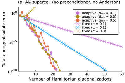
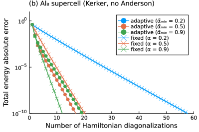
Figure 1: SCF convergence for a randomized aluminium supercell (8 atoms) without Anderson acceleration and using simple mixing (top) as well as Kerker mixing(bottom). The adaptive scheme converges robustly even in the unpreconditioned case, without requiring the manual selection of a step.

To investigate the influence of the choice of a suboptimal preconditioner on the convergence for both the fixed damping and adaptive damping strategies we considered three aluminium test systems: two elongated bulk supercells with 8 or 40 atoms as well as a surface with 40 atoms and a portion of vacuum of identical size. For the elongated supercells both the initial guess as well as the atomic positions were slightly rattled.

The results are summarized in the first segment of Table 1. For the small Al8 system, where Anderson acceleration was not used, representative convergence curves are shown in Figure 1. Due to the well-known charge-sloshing behavior, SCF iterations on such metallic systems are ill-conditioned. Without preconditioning small fixed damping values $\alpha$ are thus required to obtain convergence, with only a small window of damping values being able to achieve a convergence within 100 Hamiltonian applications. On the other hand in combination with the matching Kerker preconditioning strategy Kerker (1981) large fixed damping values generally converge more quickly.

In contrast the adaptive damping strategy is much less sensitive to the choice of the minimal trial damping $\widetilde{\alpha}_{\text{min}}$. Moreover, it leads to a much improved convergence for the case without suitable preconditioning while still maintaining similar costs if Kerker mixing is employed.

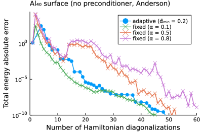
Figure 2: SCF convergence without preconditioning for an elongated supercell of an aluminium surface with 40 aluminium atom and a vacuum portion of equal size. A fixed step of $\alpha=0.1$ was optimal here, but the adaptive scheme gets very close performance without manual stepsize selection.

These observations carry over to cases including Anderson acceleration and larger aluminium systems, see Figure 2 for a representative computation on an aluminium surface. Notice that Kerker mixing is extremely badly suited for the large aluminium surface, such that convergence is not obtained in 100 Hamiltonian for any of the damping strategies, see Reference Herbst and Levitt, 2020 for a better preconditioner in such inhomogeneous systems. Overall employing adaptive damping therefore makes the reliability and efficiency of the SCF less dependent on the choice of the preconditioning strategy, while not requiring the user to manually select a damping parameter.

IV.2 Strong nonlinear effects: Gallium arsenide

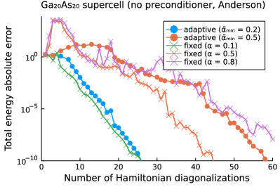
Figure 3: Elongated gallium arsenide supercell (20 gallium and 20 arsenide atoms) with slightly randomized atomic positions. For all cases, simple mixing and Anderson acceleration are employed.

In previous work we identified elongated supercells of gallium arsenide with slightly perturbed atomic positions to be a simple system that still exhibits strong nonlinear effects when the SCF is far from convergence Herbst and Levitt (2020). In the convergence profiles of these systems this manifests by the error shooting up abruptly with Anderson failing to quickly recover. In Figure 3, for example, the error increases steeply between Hamiltonian diagonalizations 3 and 6 for the fixed-damping approaches with stepsizes beyond $0.1$. It should be noted that this behavior is an artefact of the interplay of Anderson acceleration and damped SCF iterations on these systems, which is not observed in case Anderson acceleration is not employed. For more details see the discussion of the gallium arsenide case in Ref. Herbst and Levitt, 2020.

For the calculations employing a fixed damping strategy only small damping values of $\alpha=0.1$ are able to prevent this behavior. Already slightly larger damping values noticably increase the number of Hamiltonian diagonalizations required to reach convergence (compare Table 1), and thus a careful selection of the damping value is in order for such systems. In contrast the proposed adaptive damping strategy with our baseline minimal trial damping of $\widetilde{\alpha}_{\text{min}}=0.2$ automatically detects the unsuitable Anderson steps and downscales them. As a result an optimal or near-optimal cost is obtained without any manual parameter tuning. For comparison, we also display in Figure 3 the results with a large value of $\widetilde{\alpha}_{\text{min}}=0.5$, which prevents the damping algorithm to avoid the nonlinear effects.

IV.3 Challenging transition-metal compounds

In this section we discuss two types of transition-metal systems. First, we consider a selection of smaller primitive unit cells, including the mixed iron-nickel fluoride FeNiF6 as well a number of Heusler-type alloy structures, see the third group of Table 1. These structures were found found in the course of high-throughput computations to be difficult to converge Bercx and Marzari (2020). Moving to larger systems we considered an elongated chromium supercell with a single vacancy defect as well as a layered iron-tungsten system, see the fourth group of Table 1. Both test cases were taken from previous studies Winkelmann et al. (2020); Marks (2021) on SCF algorithms.

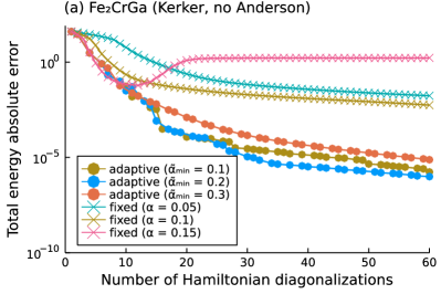
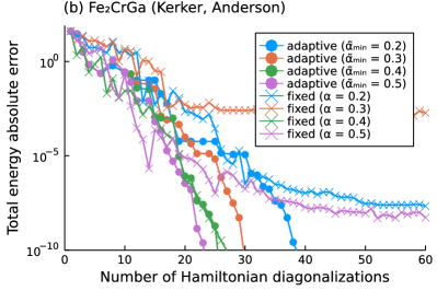
Figure 4: Convergence of the Fe2CrGa Heusler alloy with Kerker mixing without Anderson acceleration (top) and with Anderson acceleration (bottom). Notice that the SCF calculations do not necessarily converge to the same local SCF minimum.

In particular the Heusler compounds are known to exhibit rich and unusual magnetic and electronic properties. From our test set, for example, Fe2MnAl shows halfmetallic behaviour, i.e. a vanishing density of states at the Fermi level in only the minority spin channel Belkhouane et al. (2015). Other compounds, such as Mn2RuGa or CoFeMnGa show an involved pattern of ferromagnetic and antiferromagnetic coupling of the neighboring transition-metal sites Wollmann et al. (2015); Shi et al. (2020). Such effects are closely linked to the $d$-orbitals forming localized states near the Fermi level He et al. (2018); Jiang and Yang (2021) and imply that there are a multiple accessible spin configurations, which are close in energy. Unfortunately these two properties also make Heusler compounds difficult to converge using standard methods. First, localized states near the Fermi level are a source of ill-conditioning for the SCF fixed-point problem Herbst and Levitt (2020), with no cheap and widely applicable preconditioning strategy being available. Second, the abundance of multiple spin configurations implies a more involved SCF energy landscape with multiple SCF minima. On such a landscape convergence may easily “hesitate” between different local minima or stationary points. Furthermore the setup of an appropriate initial guess, which ideally guides the SCF towards the final spin ordering requires human expertise and is hard to automatise in the high-throughput setting. Albeit not fully appropriate for the systems we consider, we followed the guess setup, which has also been used in the aforementioned high-throughput procedure Bercx and Marzari (2020), namely to start the calculations with an initial guess based on ferromagnetic (FM) spin ordering.

As a result in our tests, calculations on Heusler systems without Anderson acceleration require very small fixed damping values below $0.1$ even if the Kerker preconditioner is used, see Figure 4 (a). The adaptive damping strategy improves the convergence behavior and in agreement with our previous results partially corrects for the mismatch in preconditioner and initial guess. Still, convergence is extremely slow.

An acceptable convergence is only accessible in combination with Anderson acceleration. However, the Anderson-accelerated fixed-damping SCF is very susceptible to the chosen damping $\alpha$, see Figure 4 (b). In particular the lowest-energy SCF minimum is only found within 100 Hamiltonian diagonalizations for $\alpha=0.4$, $\alpha=0.7$, $\alpha=0.8$ and $\alpha=1.0$. Other fixed damping values initially converge, but then convergence stagnates and the error only reduces very slowly beyond around $30$ diagonalizations.

We investigated the source of this pathological behavior by restarting the iterations after stagnation. This did not noticeably alter the behavior, eliminating the possibility that the history of the iterates within the Anderson acceleration scheme somehow “jam” the SCF into stagnation in the strongly nonlinear regime — as can happen for instance in nonlinear conjugate gradient methods Hager and Zhang (2006). Another possibility is that the iterations somehow got into a particularly rough region of SCF energy landscape between multiple stationary points, which is simply hard to escape. However, this is not the case either. For instance on the Fe2CrGa system with a fixed damping of $0.3$, the restarted iterations did converge quickly using an Anderson scheme with a small maximal conditioning of $10^{2}$ for the linear least squares problem. It would therefore appear that this phenomenon is due to inadequate regularization of the least squares problem. We expect more sophisticated techniques for controlling the Anderson history Chupin et al. (2020) to be worth investigating for such systems in the future.

Because of this stagnation issue we found Anderson-accelerated SCF iterations to become unreliable for our transition-metal test systems: for fixed damping values below $\alpha=0.5$, hardly any calculation converges. Notably, due to the non-trivial interplay with the Anderson scheme, this result is the exact opposite to our theoretical developments on damped SCF iterations in Section II.3, which suggested to reduce the damping to achieve reliable convergence.

Overall the transition-metal cases emphasize the difficulty in manually choosing an appropriate fixed damping. For a number of cases the window of converging damping values is rather narrow, e.g. consider Fe2CrGa, FeNiF6 or Mn3Si (with the FM guess) and in our tests only a single damping value of $\alpha=0.8$ fortitiously manages to converge all systems.

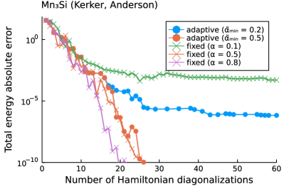
Figure 5: Convergence of the Mn3Si Heusler compound with Kerker mixing and Anderson acceleration and starting from a ferromagnetically ordered initial guess. Small dampings are susceptible to stagnation induced by Anderson instabilities.

In contrast the proposed adaptive damping strategy with our baseline value of $\widetilde{\alpha}_{\text{min}}=0.2$ is less susceptible to the stagnation issue. Across the unit cells and extended transition-metal systems we considered we observed only a convergence failure in one test case, namely the Mn3Si Heusler alloy with the FM guess, see Figure 5. For some test cases, adaptive damping did cause a noticeable computational overhead: in extreme cases (such as Fe2CrGa or Fe2MnAl) the number of required Hamiltonian diagonalizations almost doubles. However, it should be emphasized that no user adjustments were needed to obtain these results, even though adaptive damping has been constructed on the here invalid principle that smaller damping increases reliability.

Yet even on cases where Anderson instabilities cause non-convergence of the adaptive scheme, fine-tuning is possible. Increasing the minimal trial damping from $\widetilde{\alpha}_{\text{min}}=0.2$ to $\widetilde{\alpha}_{\text{min}}=0.5$, for example, increases the minimal step size and thus lowers the risk of Anderson stagnation. For all transition-metal cases we considered $\widetilde{\alpha}_{\text{min}}=0.5$ strictly reduces the number of diagonalizations required to reach convergence compared to $\widetilde{\alpha}_{\text{min}}=0.2$, see for example Figure 4 (b). Moreover this parameter adjustment even resolves the convergence issues of Mn3Si, see Figure 5. If manual intervention is possible another option is to incorporating prior knowledge of the final ground state electronic structure into the initial guess. For the Mn3Si case, for example, an improved initial guess based on an antiferromagnetic spin ordering (AFM) between adjacent manganese layers simplifies the SCF problem, such that both a larger range of fixed damping values as well as the adaptive damping strategy give rise to converging calculations.

V Conclusion

We proposed a new linesearch strategy for SCF computations, based on an efficient approximate model for the energy as a function of the damping. Our algorithm follows four general principles: (a) the algorithm should need no manual intervention from the user; (b) it should be combinable with known effective mixing techniques such as preconditioning and Anderson acceleration; (c) in “easy” cases where convergence with a fixed damping is satisfactory it should not slow down too much; and (d) it should be possible to relate it to schemes with proved convergence guarantees. We demonstrated that our proposed scheme fulfills all these objectives. With our default parameter choice of $\widetilde{\alpha}_{\text{min}}=0.2$ the resulting adaptively damped SCF algorithm is able to converge all of the “easy” cases faster or almost as fast as the fixed-damping method with the best damping. Simultaneously it is more robust than the fixed-damping method on the “hard” cases we considered, such as elongated bulk metals and metal surfaces without proper preconditioning or Heusler-type transition-metal alloys. In particular the latter kind of systems feature a very irregular convergence behavior with respect to the damping parameter, making a robust manual damping selection very challenging. In practice the classification between “easy” and “hard” cases may well depend on the considered system and the details of the computational setup, e.g. the employed mixing and acceleration techniques. However, our scheme makes no assumptions about the details how a proposed SCF step has been obtained. We therefore believe adaptive damping to be a black-box stabilisation technique for SCF iterations, which applies beyond the Anderson-accelerated setting we have considered here.

Still, our results on these “hard” cases also highlight poorly-understood limitations of the commonly used Anderson acceleration process. For example, despite following standard recommendations to increase Anderson robustness, we frequently observe SCF iterations to stagnate. A more thorough understanding of this effect would be an interesting direction for future research.

Our scheme was applied to semilocal density functionals in a plane-wave basis set. It is not specific to plane-wave basis sets, and we expect it to be similarly efficient in other “large” basis sets frequently used in condensed-matter physics. For atom-centered basis sets, like those common in quantum chemistry, direct mixing of the density matrix is feasible, and likely more efficient. Our scheme does not apply directly to hybrid functionals, where orbitals or Fock matrices have to be mixed also; an extension to this case would be an interesting direction for future research.

Appendix: mathematical proofs

Lemma 1.

Let

$$H_{*}=\sum_{i=1}^{N_{\rm b}}\varepsilon_{i}|\phi_{i}\rangle\langle\phi_{i}|$$ (48)

with orthonormal $\phi_{i}$ and non-decreasing $\varepsilon_{i}$. Let $f:{\mathbb{R}}\to{\mathbb{R}}$ be a real analytic function in a neighborhood of $[\varepsilon_{1},\varepsilon_{N_{\rm b}}]$. Then the map $H\mapsto f(H)$ is analytic in a neighborhood of $H_{*}$, and

$${\bf df}(H_{*})\cdot\delta H=\sum_{i=1}^{N_{\rm b}}\sum_{j=1}^{N_{\rm b}}\frac{f(\varepsilon_{i})-f(\varepsilon_{j})}{\varepsilon_{i}-\varepsilon_{j}}\langle\phi_{i},\delta H\phi_{j}\rangle|\phi_{i}\rangle\langle\phi_{j}|$$ (49)

with the convention that $\frac{f(\varepsilon_{i})-f(\varepsilon_{i})}{\varepsilon_{i}-\varepsilon_{i}}=f^{\prime}(\varepsilon_{i})$.

Proof of Lemma 1.  This is a classical result, known as the Daleckii-Krein theorem in linear algebra; see for instance Higham Higham (2008). To keep this paper self-contained, we follow here the proof in Levitt Levitt (2020) in the analytic case. Since $f$ is analytic on $[\varepsilon_{1},\varepsilon_{N_{\rm b}}]$, it is analytic in a complex neighborhood. Let $\mathcal{C}$ be a positively oriented contour enclosing $[\varepsilon_{1},\varepsilon_{N_{\rm b}}]$. Then, for $H$ close enough to $H_{*}$, we have

$$f(H)=\frac{1}{2\pi i}\oint_{\mathcal{C}}f(z)\frac{1}{z-H}dz$$ (50)

and analyticity of $f$ follows. For $\delta H$ small enough,

$$f(H_{*}+\delta H)$$ (51)

$$=\frac{1}{2\pi i}\oint_{\mathcal{C}}f(z)\frac{1}{z-H_{*}-\delta H}dz$$

$$\approx f(H_{*})+\frac{1}{2\pi i}\oint_{\mathcal{C}}f(z)\frac{1}{z-H_{*}}\delta H\frac{1}{z-H_{*}}dz$$

$$=f(H_{*})+\frac{1}{2\pi i}\oint_{\mathcal{C}}{}\sum_{i=1}^{N_{\rm b}}\sum_{j=1}^{N_{\rm b}}\frac{f(z)\langle\phi_{i},\delta H\phi_{j}\rangle}{(z-\varepsilon_{i})(z-\varepsilon_{j})}|\phi_{i}\rangle\langle\phi_{j}|dz$$

$$=f(H_{*})+\sum_{i=1}^{N_{\rm b}}\sum_{j=1}^{N_{\rm b}}\frac{f(\varepsilon_{i})-f(\varepsilon_{j})}{\varepsilon_{i}-\varepsilon_{j}}\langle\phi_{i},\delta H\phi_{j}\rangle|\phi_{i}\rangle\langle\phi_{j}|$$

where $\approx$ means up to terms of order $O\left(\|\delta H\|^{2}\right)$. ∎

Proof of Theorem 1.  If $\alpha_{0}\leq 1$, $H_{n}$ belongs to the convex hull spanned by $H_{0}$ and $\{H_{\rm KS}(f_{\rm FD}(H)),H\in\mathcal{H}\}$. On this compact set $X$, $f_{\rm FD}$, ${\mathcal{I}}$ and their derivatives are bounded. We have for all $H\in X$

$${\mathcal{I}}(H+\alpha(H_{\rm KS}-H))$$ (52)

$$={\mathcal{I}}(H)-\alpha\langle\bm{\Omega}^{-1}(H_{\rm KS}-H),(H_{\rm KS}-H)\rangle+O(\alpha^{2})$$

$$={\mathcal{I}}(H)-\alpha\langle\bm{\Omega}\nabla{\mathcal{I}}(H),\nabla{\mathcal{I}}(H)\rangle+O(\alpha^{2})$$

where in this expression the functions $\bm{\Omega}$ and $H_{\rm KS}$ are evaluated at $f_{\rm FD}(H)$, and the constant in the $O(\alpha^{2})$ term is uniform in $n$. It follows that for $\alpha_{0}$ small enough, there is $c>0$ such that

$${\mathcal{I}}(H_{n+1})\leq{\mathcal{I}}(H_{n})-\alpha c\|\nabla{\mathcal{I}}(H_{n})\|^{2},$$ (53)

and therefore $\nabla{\mathcal{I}}(H_{n})\to 0$, so that $H_{\rm KS}(f_{\rm FD}(H_{n}))-H_{n}\to 0$.

We now proceed as in Levitt (2012). Let ${\mathcal{I}}_{*}=\lim_{n\to\infty}{\mathcal{I}}(H_{n})$. The set $\Gamma=\{H\in X,$ ${\mathcal{I}}(H)=\lim_{n\to\infty}{\mathcal{I}}(H_{n})\}$ is non-empty and compact. Furthermore, $d(H_{n},\Gamma)\to 0$; if this was not the case, we could extract by compactness of $X$ a subsequence at finite distance of $\Gamma$ converging to a $H_{*}\in X$ satisfying ${\mathcal{I}}(H_{*})=\lim_{n\to\infty}{\mathcal{I}}(H_{n})$, which would imply that $H_{*}\in\Gamma$, a contradiction.

At every point $H$ of $\Gamma$, by analyticity there is a neighborhood of $H$ in $\mathcal{H}$ such that the Łojasiewicz inequality

$$|{\mathcal{I}}(H^{\prime})-{\mathcal{I}}_{*}|^{1-\theta_{H}}\leq\kappa_{H}\|\nabla{\mathcal{I}}(H^{\prime})\|$$ (54)

holds for some constants $\theta_{H}\in(0,1/2]$, $\kappa_{H}>0$ Levitt (2012); Lojasiewicz (1965). By compactness, we can extract a finite covering of these neighborhoods, and obtain a Łojasiewicz inequality with universal constants $\theta\in(0,1/2],\kappa>0$ in a neighborhood of $\Gamma$. Therefore, for $n$ large enough, using the concavity inequality $x^{\theta}\leq y^{\theta}+\theta y^{\theta-1}(x-y)$ with $x={\mathcal{I}}(H_{n+1})-{\mathcal{I}}_{*}$, $y={\mathcal{I}}(H_{n})-{\mathcal{I}}_{*}$, we get

$$\|\nabla{\mathcal{I}}(H_{n})\|^{2} \leq\frac{1}{\alpha c}{{\mathcal{I}}(H_{n})-{\mathcal{I}}(H_{n+1})}$$ (55)

$$\leq\frac{1}{\theta\alpha c}({\mathcal{I}}(H_{n})-{\mathcal{I}}_{*})^{1-\theta}$$

$$\hskip 28.45274pt\cdot\Big{[}\left({\mathcal{I}}(H_{n})-{\mathcal{I}}_{*}\right)^{\theta}-({\mathcal{I}}(H_{n+1})-{\mathcal{I}}_{*})^{\theta}\Big{]}$$

$$\leq\frac{\kappa}{\theta\alpha c}\|\nabla{\mathcal{I}}(H_{n})\|$$

$$\hskip 28.45274pt\cdot\Big{[}({\mathcal{I}}(H_{n})-{\mathcal{I}}_{*})^{\theta}-({\mathcal{I}}(H_{n+1})-{\mathcal{I}}_{*})^{\theta}\Big{]}$$

$$\|\nabla{\mathcal{I}}(H_{n})\| \leq\frac{\kappa}{\theta\alpha c}\Big{[}({\mathcal{I}}(H_{n})-{\mathcal{I}}_{*})^{\theta}-({\mathcal{I}}(H_{n+1})-{\mathcal{I}}_{*})^{\theta}\Big{]}$$

It follows that $\|\nabla{\mathcal{I}}(H_{n})\|$ is summable, and therefore that $\|H_{n+1}-H_{n}\|$ is; this implies convergence of $H_{n}$ to some $H_{*}$. When $\theta=1/2$ (or, in light of (22), when $\bm{d^{2}{\mathcal{E}}}(f_{\rm FD}(H_{*}))$ is positive definite), we can get exponential convergence Levitt (2012). ∎

Note that the bounds used in the proof of the above statement (for instance, on $\alpha_{0}$) are extremely pessimistic, since they rely on the fact that the set of possible $P$ is bounded, and therefore all density matrices of the form $f_{\rm FD}(H_{\rm KS}(P))$ have occupations bounded away from $0$ and $1$, which results in bounded derivatives for ${\rm Tr}(s(P))$. A more careful analysis is needed to obtain better bounds (for instance, bounds that are better behaved in the zero temperature limit).

Proof of Theorem 2. From (52) it is easily seen that the linesearch process stops in a finite number of iterations, independent on $n$. This ensures that there is $\alpha_{\rm min}>0$ such that $\alpha_{\rm min}\leq\alpha_{n}\leq\alpha_{\rm max}$. From (26) it follows that a similar inequality to (53) holds, and the rest of the proof proceeds as in that of Theorem 1.

References

- Woods et al. (2019) N. D. Woods, M. C. Payne, and P. J. Hasnip, Journal of Physics: Condensed Matter 31, 453001 (2019).
- Lehtola et al. (2020) S. Lehtola, F. Blockhuys, and C. Van Alsenoy, Molecules 25, 1218 (2020).
- Jain et al. (2016) A. Jain, Y. Shin, and K. A. Persson, Nature Reviews Materials 1 (2016), 10.1038/natrevmats.2015.4.
- Alberi et al. (2019) K. Alberi, M. B. Nardelli, A. Zakutayev, L. Mitas, S. Curtarolo, A. Jain, M. Fornari, N. Marzari, I. Takeuchi, M. L. Green, M. Kanatzidis, M. F. Toney, S. Butenko, B. Meredig, S. Lany, U. Kattner, A. Davydov, E. S. Toberer, V. Stevanovic, A. Walsh, N.-G. Park, A. Aspuru-Guzik, D. P. Tabor, J. Nelson, J. Murphy, A. Setlur, J. Gregoire, H. Li, R. Xiao, A. Ludwig, L. W. Martin, A. M. Rappe, S.-H. Wei, and J. Perkins, Journal of Physics D: Applied Physics 52, 013001 (2019).
- Luo et al. (2021) S. Luo, T. Li, X. Wang, M. Faizan, and L. Zhang, WIREs Computational Molecular Science 11 (2021), 10.1002/wcms.1489.
- Curtarolo et al. (2012) S. Curtarolo, W. Setyawan, G. L. Hart, M. Jahnatek, R. V. Chepulskii, R. H. Taylor, S. Wang, J. Xue, K. Yang, O. Levy, M. J. Mehl, H. T. Stokes, D. O. Demchenko, and D. Morgan, Computational Materials Science 58, 218 (2012).
- Jain et al. (2011) A. Jain, G. Hautier, C. J. Moore, S. Ping Ong, C. C. Fischer, T. Mueller, K. A. Persson, and G. Ceder, Computational Materials Science 50, 2295 (2011).
- Huber et al. (2020) S. P. Huber, S. Zoupanos, M. Uhrin, L. Talirz, L. Kahle, R. Häuselmann, D. Gresch, T. Müller, A. V. Yakutovich, C. W. Andersen, F. F. Ramirez, C. S. Adorf, F. Gargiulo, S. Kumbhar, E. Passaro, C. Johnston, A. Merkys, A. Cepellotti, N. Mounet, N. Marzari, B. Kozinsky, and G. Pizzi, Scientific Data 7 (2020), 10.1038/s41597-020-00638-4.
- Feng and Cameron (2007) W. Feng and K. Cameron, Computer 40, 50 (2007).
- Feng et al. (2008) W. Feng, X. Feng, and R. Ge, IT Professional 10, 17 (2008).
- Herbst and Levitt (2020) M. F. Herbst and A. Levitt, Journal of Physics: Condensed Matter (2020), 10.1088/1361-648x/abcbdb.
- Cancès (2000) E. Cancès, “SCF algorithms for HF electronic calculations,” (Springer Berlin Heidelberg, 2000) pp. 17–43.
- Cancès and Le Bris (2000) E. Cancès and C. Le Bris, International Journal of Quantum Chemistry 79, 82 (2000).
- Kudin et al. (2002) K. N. Kudin, G. E. Scuseria, and E. Cancès, The Journal of Chemical Physics 116, 8255 (2002), http://aip.scitation.org/doi/pdf/10.1063/1.1470195 .
- Francisco et al. (2004) J. B. Francisco, J. M. Martınez, and L. Martınez, The Journal of chemical physics 121, 10863 (2004).
- Francisco et al. (2006) J. B. Francisco, J. M. Martínez, and L. Martínez, Journal of Mathematical Chemistry 40, 349 (2006).
- Cancès et al. (2021) E. Cancès, G. Kemlin, and A. Levitt, SIAM Journal on Matrix Analysis and Applications 42, 243 (2021).
- Marzari et al. (1997) N. Marzari, D. Vanderbilt, and M. C. Payne, Physical Review Letters 79, 1337 (1997).
- Freysoldt et al. (2009) C. Freysoldt, S. Boeck, and J. Neugebauer, Physical Review B 79, 241103 (2009).
- Marks (2021) L. D. Marks, Journal of Chemical Theory and Computation 17, 5715 (2021).
- Marks and Luke (2008) L. Marks and D. Luke, Physical Review B 78, 075114 (2008).
- Gonze (1996) X. Gonze, Physical Review B 54, 4383 (1996).
- Mermin (1965) N. D. Mermin, Physical Review 137, A1441 (1965).
- Methfessel and Paxton (1989) M. Methfessel and A. Paxton, Physical Review B 40, 3616 (1989).
- Adler (1962) S. L. Adler, Physical Review 126, 413 (1962).
- Wiser (1963) N. Wiser, Physical Review 129, 62 (1963).
- Dederichs and Zeller (1983) P. H. Dederichs and R. Zeller, Physical Review B 28, 5462 (1983).
- Kerker (1981) G. P. Kerker, Physical Review B 23, 3082 (1981).
- Walker and Ni (2011) H. Walker and P. Ni, SIAM Journal on Numerical Analysis 49, 1715 (2011), https://doi.org/10.1137/10078356X .
- Chupin et al. (2020) M. Chupin, M.-S. Dupuy, G. Legendre, and E. Séré, (2020), 2002.12850v1 .
- Saad (2003) Y. Saad, Iterative Methods for Sparse Linear Systems, 2nd ed., edited by Y. Saad (SIAM Publishing, 2003).
- Kresse and Furthmüller (1996) G. Kresse and J. Furthmüller, Physical Review B 54, 11169 (1996).
- Herbst et al. (2021) M. F. Herbst, A. Levitt, and E. Cancès, Proc. JuliaCon Conf. 3, 69 (2021).
- Herbst and Levitt (2021a) M. F. Herbst and A. Levitt, “Density-functional toolkit (DFTK), version v0.3.10,” (2021a), https://dftk.org.
- Perdew et al. (1996) J. P. Perdew, K. Burke, and M. Ernzerhof, Physical Review Letters 77, 3865 (1996).
- Lehtola et al. (2018) S. Lehtola, C. Steigemann, M. J. Oliveira, and M. A. Marques, SoftwareX 7, 1 (2018).
- Goedecker et al. (1996) S. Goedecker, M. Teter, and J. Hutter, Physical Review B 54, 1703 (1996).
- Herbst and Levitt (2021b) M. F. Herbst and A. Levitt, “Computational scripts and raw data for the presented numerical tests,” (2021b), https://github.com/mfherbst/supporting-adaptive-damping.
- Bercx and Marzari (2020) M. Bercx and N. Marzari, Private communication (2020).
- Winkelmann et al. (2020) M. Winkelmann, E. Di Napoli, D. Wortmann, and S. Blügel, Physical Review B 102 (2020), 10.1103/physrevb.102.195138.
- Belkhouane et al. (2015) M. Belkhouane, S. Amari, A. Yakoubi, A. Tadjer, S. Méçabih, G. Murtaza, S. Bin Omran, and R. Khenata, Journal of Magnetism and Magnetic Materials 377, 211 (2015).
- Wollmann et al. (2015) L. Wollmann, S. Chadov, J. Kübler, and C. Felser, Physical Review B 92 (2015), 10.1103/physrevb.92.064417.
- Shi et al. (2020) B. Shi, J. Li, C. Zhang, W. Zhai, S. Jiang, W. Wang, D. Chen, Y. Yan, G. Zhang, and P.-F. Liu, Physical Chemistry Chemical Physics 22, 23185 (2020).
- He et al. (2018) J. He, S. S. Naghavi, V. I. Hegde, M. Amsler, and C. Wolverton, Chemistry of Materials 30, 4978 (2018).
- Jiang and Yang (2021) S. Jiang and K. Yang, Journal of Alloys and Compounds 867, 158854 (2021).
- Hager and Zhang (2006) W. W. Hager and H. Zhang, Pacific Journal of Optimization 2, 35 (2006).
- Higham (2008) N. J. Higham, Functions of matrices: theory and computation (SIAM, 2008).
- Levitt (2020) A. Levitt, Archive for Rational Mechanics and Analysis 238, 901 (2020).
- Levitt (2012) A. Levitt, ESAIM: Mathematical Modelling and Numerical Analysis 46, 1321 (2012).
- Lojasiewicz (1965) S. Lojasiewicz, Lectures Notes IHES (Bures-sur-Yvette) (1965).