ParSNIP: Generative Models of Transient Light Curves with Physics-Enabled Deep Learning

Abstract

We present a novel method to produce empirical generative models of all kinds of astronomical transients from datasets of unlabeled light curves. Our hybrid model, that we call ParSNIP, uses a neural network to model the unknown intrinsic diversity of different transients and an explicit physics-based model of how light from the transient propagates through the universe and is observed. The ParSNIP model predicts the time-varying spectra of transients despite only being trained on photometric observations. With a three-dimensional intrinsic model, we are able to fit out-of-sample multiband light curves of many different kinds of transients with model uncertainties of 0.04–0.06 mag. The representation learned by the ParSNIP model is invariant to redshift, so it can be used to perform photometric classification of transients even with heavily biased training sets. Our classification techniques significantly outperform state-of-the-art methods on both simulated (PLAsTiCC) and real (PS1) datasets with 2.3$\times$ and 2$\times$ less contamination respectively for classification of Type Ia supernovae. We demonstrate how our model can identify previously-unobserved kinds of transients and produce a sample that is 90% pure. The ParSNIP model can also estimate distances to Type Ia supernovae in the PS1 dataset with an RMS of $0.150\pm 0.007$ mag compared to $0.155\pm 0.008$ mag for the SALT2 model on the same sample. We discuss how our model could be used to produce distance estimates for supernova cosmology without the need for explicit classification.

1 Introduction

Upcoming surveys such as the Legacy Survey of Space and Time (LSST; Ivezić et al., 2019) that will be conducted at the Vera C. Rubin Observatory, and the Nancy Grace Roman Space Telescope (Spergel et al., 2015) will obtain light curves for millions of astronomical transients. These large datasets will enable many novel science applications. The number of observed Type Ia supernovae (SNe Ia) will increase by more than two orders of magnitude compared to current samples (LSST Science Collaboration et al., 2009; Scolnic et al., 2018). These large samples of SNe Ia will be used to constrain cosmological parameters both by improving measurements of the expansion history of the universe and by performing novel measurements of local peculiar velocity field (Graziani et al., 2020). These surveys will also observe large numbers of other kinds of transients, such as superluminous supernovae (SLSN), which will be helpful both to elucidate the origins of these transients (Villar et al., 2018) and to use them as new cosmological probes (Scovacricchi et al., 2016). It is also likely that new kinds of rare transients that have not previously been observed will be discovered in the datasets from these surveys.

All of these science applications rely on being able to extract information from light curves and distinguish between light curves of different kinds of transients. Observations can be compared directly to simulations and theory (Kerzendorf et al., 2021), but these models are not currently accurate enough to characterize observed light curves at the precision required for many science applications. For SNe Ia, a range of different empirical models have been created to describe their light curves and spectra (Guy et al., 2007; Saunders et al., 2018; Léget et al., 2020; Mandel et al., 2020). These are generative models in that they predict the full time-varying spectrum of a transient in terms of a small number of parameters whose distribution is reasonably well known.

These models all include explicit descriptions of how the light propagates through the universe and is observed on a detector. Propagation effects include redshifting of the light from the transient, dust along the line of sight, and luminosity variation due to effects such as weak gravitational lensing. A light curve can be observed with different cadences, with different telescopes, in different bandpasses, at different signal-to-noises, or at different times. All of these effects will change the observed light curve for a transient, but they do not affect the intrinsic physics of the underlying transient. We therefore refer to them as “symmetries”. By explicitly handling these symmetries, the previously-described models of SNe Ia obtain consistent values of the model parameters when fitting light curves observed under different conditions. In particular, these models can obtain consistent estimates of the luminosity when fitting light curves at different redshifts which is essential for estimating distances to SNe Ia.

Similar models do not exist for other kinds of transients. Instead, previous work using light curves of non-SNe Ias has typically focused on extracting features from the light curves rather than building a generative model. Features can be extracted by fitting an empirical functional form to the light curve (Bazin et al., 2009; Sanders et al., 2015), by fitting parameters of a theoretical model to match the light curve (Guillochon et al., 2018), by estimating a smooth approximation to the light curve from which arbitrary empirical features can be measured (Lochner et al., 2016; Boone, 2019; Alves et al., 2021), or by using a neural network (Muthukrishna et al., 2019; Möller & de Boissière, 2020). These methods produce a large number of features that can be used to characterize a given light curve, but these features are not typically invariant to the symmetries of how the light curve was observed. In particular, the features produced by all of these models tend to be highly dependent on redshift. This is a major challenge for science applications such as photometric classification where labeled datasets tend to be heavily biased towards bright, low-redshift transients (Lochner et al., 2016; Boone, 2019).

In this work, we address these challenges by building a generative model of all transient light curves that is invariant to observing conditions. Most techniques that have previously been used to build generative models of SNe Ia assume that the diversity of SNe Ia can be described by a simple linear model. Such models provide a good description of most normal SNe Ia, but they fail to describe peculiar SNe Ia (Boone et al., 2021a, b) and are not flexible enough to describe most other kinds of transients. Furthermore, the techniques used to build these models require large datasets of well-measured light curves and spectra (Betoule et al., 2014) that are not available for transients other than SNe Ia.

Instead, we learn a generative model directly from large samples of light curves using a modified version of a variational autoencoder (VAE; Kingma & Welling, 2014). A VAE learns a low-dimensional representation of its input that we call a latent space. First, an encoder model uses variational inference to approximate the posterior distribution over the latent space for a given input. A generative model, also referred to as a decoder, then reconstructs the input given a point in the latent space. The VAE can be trained by applying both the encoder and decoder to a given input and by comparing the original input to the reconstructed one.

Autoencoders have previously been applied to astronomical light curves (Naul et al., 2018; Pasquet et al., 2019; Martínez-Palomera et al., 2020; Villar et al., 2020, 2021) and shown to be effective for tasks such as photometric classification and outlier identification. However, these models do not include explicit descriptions of observing symmetries, so the same transient observed under different conditions (e.g. redshift) will be assigned to different locations in the latent space. In this work, we produce a hybrid physics-VAE model where we use a neural network to describe the intrinsic time-varying spectra of astronomical transients and an explicit physical model for known symmetries. Our model produces a three-dimensional representation of the intrinsic diversity of transients that is insensitive to observing conditions, including redshift. We call the resulting model “ParSNIP” (Parameterization of SuperNova Intrinsic Properties).

We describe the datasets that we use for this work in Section 2. In Section 3, we describe the ParSNIP model and how it is trained. We evaluate the performance of the ParSNIP model as a generative model in Section 4 and show how it is able to learn the full time-varying spectra for transients despite only being trained on light curve data. In Section 5, we show how the ParSNIP model achieves state-of-the-art performance for tasks such as photometric classification, identification of new transients, or cosmological distance estimation. Finally, in Section 6 we discuss how the ParSNIP model can be applied to other datasets and how it could be improved.

2 Dataset

We evaluate the techniques described in this work on two different datasets of supernova-like light curves. First, we use a dataset of observed supernova-like light curves from the Pan-STARRS1 Medium-Deep Survey (PS1) (Chambers et al., 2016), the details of which are described in Villar et al. (2020). This dataset contains 2,885 light curves with host-galaxy redshifts of which 557 have spectroscopically-confirmed types. The light curves were observed in the Pan-STARRS g, r, i, and z bandpasses with a cadence of $\sim$7 days per filter.

We also evaluate the ParSNIP model on the PLAsTiCC dataset of simulated light curves described in (Kessler et al., 2019). This dataset contains 3,006,109 simulated supernova-like light curves with observations in the Rubin Observatory’s u, g, r, i, z, and y bandpasses, and the authors aimed to simulate a realistic dataset of light curves from three years of operation of the Rubin Observatory. This simulation consists of two distinct surveys. The vast majority of the light curves (2,972,316) are from the Wide-Fast-Deep (WFD) survey which covers around half of the sky with observations roughly twice per week in at least one of the six bandpasses. 33,793 light curves are from the Deep-Drilling-Fields (DDF) survey which covers $\sim$50 deg² with significantly deeper and more frequent observations. The authors of the PLAsTiCC dataset also simulated a spectroscopic followup strategy which produces type labels for 5,153 of the light curves in this dataset. This labeled dataset is highly biased towards bright transients, and has a mean redshift of 0.32 compared to 0.50 for the full dataset.

For this analysis, we assume that the redshifts of all of the transients are known. This assumption is not required for our analysis, but it does simplify our methodology. We will discuss how our methods can be applied to datasets where the redshift is not available in Section 6.3.

We restrict our analysis to supernova-like light curves. By this, we mean that we consider any extragalactic light curves where there is an excess of flux for a single well-defined time period, and where the light curve has a stable background level before and after this time period. The PS1 dataset that we use was already restricted to these kinds of light curves. For the PLAsTiCC dataset, we reject all of the galactic and AGN light curves but keep all other kinds of transients.

2.1 Preprocessing

To preprocess our light curves, we first make a rough estimate of the time of maximum light of the light curve by taking the median time of the five highest signal-to-noise observations in the light curve. In each bandpass, we estimate the background level using a biweight estimator (Beers et al., 1990) on all observations at least 250 days from our estimated time of maximum light. We subtract this estimate of the background level from each light curve. For the PS1 dataset, we also correct the light curves for Milky Way extinction using the dust map from Schlafly & Finkbeiner (2011).

Neural networks typically perform better if their inputs have a limited range, but flux values can vary over many orders of magnitude. To address this, we normalize the brightness of each light curve by its maximum flux in observations in any band with a signal-to-noise of at least five. After this procedure, most flux values lie between zero and one. We record the normalization scale, and use it in future analyses such as distance estimation.

We find that the statistical uncertainties that are reported for both the PLAsTiCC and PS1 datasets heavily underestimate the true uncertainties for very high signal-to-noise observations. This is partially due to uncertainties in our background subtraction procedure. To prevent these underestimated uncertainties from having excessively large weights in our model, we add an error floor of 0.01 to all of our flux uncertainties when training the model. With our normalization, this roughly corresponds to an error floor of 1% of the peak flux.

Astronomical light curves are typically sparsely sampled, but most neural network architectures require inputs that are sampled on an evenly-spaced grid. To be able to use these architectures, we evaluate our light curves on a grid following a procedure similar to the one described in Pasquet et al. (2019). Note that astronomical observations from a given telescope typically only occur during a short time interval each night when the target is near the zenith. All observations of the same target will be separated in time by some integer number of sidereal days with residuals of only $\sim$1 hour. We can therefore evaluate the light curve on a grid of sidereal days and preserve almost all of the temporal information.

For each transient, we build a grid of observations that has a length of 300 sidereal days centered on the estimated time of maximum light. The grid has rows for the flux and inverse flux variance in each bandpass. For nights where the transient was observed in a given bandpass, we include the observed flux value and inverse flux variance in the grid. For nights when the transient was not observed, we simply input zero for both the flux and inverse flux variance. We also include one row in the grid for the redshift, with the same value repeated at all times. After this procedure, our light curves are represented by a two-dimensional grid of size $300\times(2N+1)$ where $N$ is the number of bandpasses that we are modeling. We can then use standard neural network architectures to process our light curves.

3 Methods

3.1 Overview

The overall design goal for our model is to build a representation of the diversity of transients that disentangles intrinsic diversity related to the physics of the transient from diversity related to the symmetries of how the transient was observed. A transient should be assigned the same intrinsic representation regardless of how it was observed. In particular, we would like for out model to be invariant to redshift, meaning that a transient is assigned the same intrinsic representation regardless of the redshift that it is observed at.

Many different approaches exist for modeling disentangled representations with autoencoders (Tschannen et al., 2018). These approaches mostly rely on either using a supervised training procedure (which would require labels that we do not have) (e.g. Kulkarni et al., 2015) or using regularization to encourage an implicit disentangled representation (e.g. Higgins et al., 2017). We adopt an approach similar to that of spatial-VAE (Bepler et al., 2019) where we generate a disentangled representation by explicitly including known symmetries in our generative model.

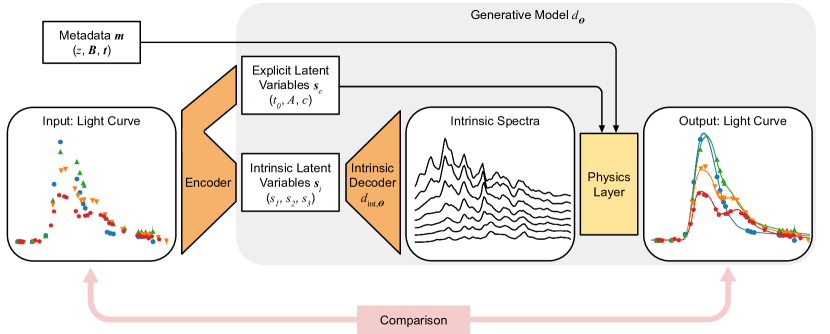
Our generative model first uses a neural network to predict the intrinsic spectra of a given transient as a function of three intrinsic latent variables. The intrinsic spectra are then passed through a physics layer that explicitly models how the light propagates through the universe and is observed. The physics layer also takes as input a set of explicit latent variables and metadata describing the observing conditions. A schematic overview of our model is shown in Figure 1.

Figure 1: Schematic overview of the ParSNIP model. An encoder model predicts the posterior distribution over a set of latent variables for a given input light curve. We label a subset of these latent variables as intrinsic latent variables, and use them as input to an intrinsic decoder model that predicts the full intrinsic time-varying spectrum of the transient. A physics layer then describes how light propagates through the universe and is observed on a detector. The physics layer takes as input a set of explicit latent variables and metadata describing the observing conditions. The encoder and intrinsic decoder are implemented as neural networks. The physics layer uses only physical relations with known functional forms and it has no free model parameters.

3.2 Variational Autoencoders

To build this model, we developed a modified version of a VAE (Kingma & Welling, 2014). As traditionally formulated, a VAE is used to model some observed random variables $\bm{y}$ in terms of some unobserved random variables $\bm{s}$. We assume that $\bm{s}$ are drawn from some prior distribution $p_{\bm{\theta}}(\bm{s})$, and that $\bm{y}$ are then drawn from the conditional distribution $p_{\bm{\theta}}(\bm{y}|\bm{s})$. These distributions are assumed to be part of some family of distributions parameterized by the hyperparameters $\bm{\theta}$.

The posterior distribution $p_{\bm{\theta}}(\bm{s}|\bm{y})$ is in general intractable. Instead of modeling it directly, in a VAE we instead assume that the posterior can be parameterized using some family of distributions $q_{\bm{\phi}}(\bm{s}|\bm{y})$ with hyperparameters $\bm{\phi}$. As shown in Kingma & Welling (2014), the marginal likelihood of a given observation $\bm{y}$ is then bounded by:

$$\log p_{\bm{\theta}}(\bm{y}) \geq\mathbb{E}_{q_{\bm{\phi}}(\bm{s}|\bm{y})}\left[\log p_{\bm{\theta}}(\bm{y}|\bm{s})\right]$$

$$\indent-D_{KL}(q_{\bm{\phi}}(\bm{s}|\bm{y})||p_{\bm{\theta}}(\bm{s}))$$ (1)

The right side of this equation is referred to as the “evidence lower bound” or ELBO. The first term of the ELBO captures the likelihood of the data under our model, and can be interpreted as the reconstruction error of the model. The second term represents the Kullback-Leibler divergence (Kullback & Leibler, 1951) between the approximate posterior $q_{\bm{\phi}}(\bm{s}|\bm{y})$ and the prior $p_{\bm{\theta}}(\bm{s})$, and is effectively a constraint on the form of the approximate posterior.

Typically, an isotropic multivariate Gaussian is assumed for the prior over the latent representation $\bm{s}$:

$$p_{\bm{\theta}}(\bm{s})=\mathcal{N}(\bm{0},\bm{I})$$ (2)

and $p_{\bm{\theta}}(\bm{y}|\bm{s})$ is assumed to be described by a Gaussian distribution with a diagonal covariance matrix whose mean is given by some deterministic function $d_{\theta}(\bm{s})$:

$$p_{\bm{\theta}}(\bm{y}|\bm{s})=\mathcal{N}(d_{\bm{\theta}}(\bm{s}),\sigma_{\bm{y}}^{2}\bm{I})$$ (3)

Finally, we assume that $q_{\bm{\phi}}(\bm{s}|\bm{y})$ is described by a Gaussian distribution with a diagonal covariance matrix:

$$q_{\bm{\phi}}(\bm{s}|\bm{y})=\mathcal{N}(\mu_{\bm{\phi}}(\bm{y}),\sigma_{\bm{\phi}}(\bm{y})^{2}\bm{I})$$ (4)

where $\mu_{\bm{\phi}}(\bm{y})$ and $\sigma_{\bm{\phi}}(\bm{y})$ are some deterministic functions of $\bm{y}$. The validity of this assumption will be discussed in Section 6.5.

Training a VAE then consists of finding appropriate functions for $d_{\bm{\theta}}(\bm{s})$, $\mu_{\bm{\phi}}(\bm{y})$, and $\sigma_{\bm{\phi}}(\bm{y})$ that maximize the ELBO in Equation 1. These functions are typically implemented as neural networks. A VAE has an architecture that resembles a classical autoencoder. The function $\mu_{\bm{\phi}}(\bm{y})$ is analogous to the encoder that takes a set of observations $\bm{y}$ and outputs a location in the latent representation $\bm{s}$. $d_{\bm{\theta}}(\bm{s})$ can be interpreted as a decoder that generates a forward model of the observations from the latent representation. The full decoder model of the VAE given by

$$p_{\bm{\theta}}(\bm{y},\bm{s})=p_{\bm{\theta}}(\bm{y}|\bm{s})p_{\bm{\theta}}(\bm{s})$$ (5)

is a generative model.

3.3 Incorporating Symmetries into Variational Autoencoders

In this work we modify the standard VAE architecture to explicitly incorporate symmetries into our model. Note that the functions $d_{\bm{\theta}}(\bm{s})$, $\mu_{\bm{\phi}}(\bm{y})$, and $\sigma_{\bm{\phi}}(\bm{y})$ are arbitrary functions. Rather than implementing these purely as neural networks, we instead use a hybrid implementation where we explicitly model symmetries of the observations where the functional form is known, and where we use neural networks for parts of the model whose functional forms are a priori unknown.

Formally, we identify the subset of latent variables that represent known symmetries of the model as “explicit latent variables”, and we label them $\bm{s}_{e}$. We call the remaining latent variables that represent diversity whose functional form is unknown “intrinsic latent variables”, and we label them $\bm{s}_{i}$. Then $\bm{s}=\{\bm{s}_{e},\bm{s}_{i}\}$. We also allow for additional metadata of the observations $\bm{m}$ that describe known observing conditions (e.g. the time that an observation was taken at). With these definitions, we model the decoder as

$$d_{\bm{\theta}}(\bm{s}_{i},\bm{s}_{e},\bm{m})=f_{1}(\bm{s}_{e},\bm{m},d_{\text{int},\bm{\theta}}(f_{2}(\bm{s}_{e},\bm{s}_{i},\bm{m})))$$ (6)

where $d_{\text{int},\bm{\theta}}$ is an arbitrary function that models the intrinsic diversity. $f_{1}$ and $f_{2}$ are fixed functions that apply known symmetries to the inputs and outputs of $d_{\text{int},\bm{\theta}}$.

To model transient light curves, we choose to use explicit functional forms for the amplitude of the light curve $A$, the color (capturing dust reddening of the light curve) $c$, and a reference time for the light curve $t_{0}$. Each observation also has associated metadata for the redshift of the light curve $z$, the time of the observation $\bm{t}$, and the bandpass that was used for the observation $\bm{B}(\lambda)$. In our formalism, we have $\bm{s}_{e}=\{A,c,t_{0}\}$ and $\bm{m}=\{z,\bm{t},\bm{B}(\lambda)\}$. We incorporate the known effects of each of these terms on astronomical observations into the $f_{1}$ and $f_{2}$ functions to produce the following decoder

$$d_{\bm{\theta}}(\bm{s}_{i},A,c,t_{0},z,\bm{t},\bm{B}(\lambda))$$ (7)

$$=\int d\lambda\cdot A\cdot\bm{B}(\lambda)\cdot C(c,\frac{\lambda}{1+z})\cdot d_{\text{int},\bm{\theta}}\left(\frac{\bm{t}-t_{0}}{1+z},\frac{\lambda}{1+z},\bm{s}_{i}\right)$$

where $C(c,\lambda)$ is a fixed dust extinction law that is applied in the rest frame, and $\bm{B}(\lambda)$ are the bandpasses used for each observation with known throughput. We choose to use the color law $C(c,\lambda)$ from Fitzpatrick & Massa (2007) in this work with $R_{V}=3.1$ as implemented in the extinction package (Barbary, 2016). $d_{\text{int},\bm{\theta}}$ is then effectively modeling the time-evolution of the rest frame spectrum of the transient.

The SALT2 model that is often used to fit SNe Ia (Guy et al., 2007) is actually a special case of the general model described in Equation 7 with the a single intrinsic latent parameter $x_{1}$ describing the width of the light curve, i.e. $\bm{s}_{i}=\{x_{1}\}$. For SALT2, the intrinsic diversity is modeled by a linear sum of two spline template functions $M_{0}(\lambda,t)$ and $M_{1}(\lambda,t)$:

$$d_{\text{int},\text{SALT2}}(\bm{t},\lambda,x_{1})=M_{0}(\lambda,\bm{t})+x_{1}M_{1}(\lambda,\bm{t})$$ (8)

The SALT2 model provides a good description of most SNe Ia, but its model of intrinsic diversity is linear which is insufficient for some SNe Ia (Boone et al., 2021a, b) and most other kinds of transients.

3.4 Modeling Spectra with a Neural Network

In order to model a wide range of transients, we choose to implement $d_{\text{int},\bm{\theta}}$ as a multilayer perceptron (MLP). This function takes as input both the time of an observation and the intrinsic latent variables $\bm{s}_{i}$. A large part of the spectrum is typically needed to compute bandpass photometry, so for computational reasons we choose to predict the full restframe spectrum with the MLP on a grid of wavelength elements rather than having the wavelength as an additional input. Synthetic photometry can then be computed by numerically evaluating the integral in Equation 7. Labeling the index of each restframe wavelength bin as $n$, our implementation of the decoder can then be written as

$$d_{\bm{\theta}}(\bm{s}_{i},A,c,t_{0},z,\bm{t},\bm{B}(\lambda))$$ (9)

$$=\sum_{n}A\cdot\bm{B}^{\prime}_{n}\cdot C(c,\lambda^{\prime}_{n})\cdot d_{\text{int},\bm{\theta},n}\left(\frac{\bm{t}-t_{0}}{1+z},\bm{s}_{i}\right)$$

Here $\lambda^{\prime}_{n}$ is the central rest-frame wavelength for bin $n$. $\bm{B}^{\prime}_{n}$ are the integrated bandpasses for bin $n$ which can be computed by integrating the bandpasses over each wavelength bin

$$\bm{B}^{\prime}_{n}=\int_{\lambda^{\prime}_{n,\text{min}}}^{\lambda^{\prime}_{n,\text{max}}}d\lambda\cdot\bm{B}((1+z)\lambda)$$ (10)

We choose to use a grid of 300 spectral elements with rest frame wavelengths that are logarithmically-spaced between 1,000 and 11,000 Å. Logarithmically-spaced wavelength elements simplify computing the integrated bandpasses $\bm{B}^{\prime}_{n}$ because redshifting the bandpass is equivalent to a translation of the wavelength elements. We precompute the integrated bandpasses $\bm{B}^{\prime}_{n}$ by numerically evaluating the integral in Equation 10 with 51 times oversampling. With this configuration, we find that the numerical uncertainties in our synthetic photometry are $\sim$0.0002 mag which is much smaller than typical measurement uncertainties.

To summarize, we implement $d_{\text{int},\bm{\theta}}$ as an MLP that takes as inputs the intrinsic latent variables $\bm{s}_{i}$ and a time. The output of this MLP is a restframe spectrum on a grid of 300 spectral elements. We then use an explicit physics model of host-galaxy dust, redshift, and the bandpasses of the telescope to calculate synthetic photometry from the predicted spectrum and compare with observations. The MLP has several hyperparameters, namely the number of layers, width of each layer, and activation function. The values of these hyperparameters will be discussed in Section 3.11.

With this architecture, the full decoder model $d_{\bm{\theta}}$ naturally handles all of the previously-described symmetries of how the transient was observed. We can evaluate the full model in different bandpasses or at different redshifts without making any changes to the intrinsic model or to the intrinsic latent variables $\bm{s}_{i}$. This is a major difference from previous autoencoder models that predict the light curve in specific bands directly, and that therefore have a representation where the intrinsic properties are entangled with properties of how the observations were taken (e.g. Pasquet et al., 2019; Villar et al., 2020).

3.5 Symmetry-Aware Encoders

We choose to model the posterior distribution of the latent variables for a given light curve as a Gaussian distribution with a diagonal covariance matrix, as shown in Equation 4. We assume a $\mathcal{N}(\bm{0},\bm{I})$ prior for the intrinsic latent variables. For the color $c$, we assume a weak prior of $\mathcal{N}(0,0.3^{2})$ which is much larger than the true dust distribution. Similarly, we assume a weak prior of $\mathcal{N}(0,(20~{}\text{days})^{2})$ for the reference time $t_{0}$ which should be much wider than the uncertainty from the estimated times of maximum light from the preprocessing step in Section 2.1. As will be discussed in Section 3.7, we marginalize over the amplitude and evaluate its posterior directly so it is ultimately not predicted by our encoder.

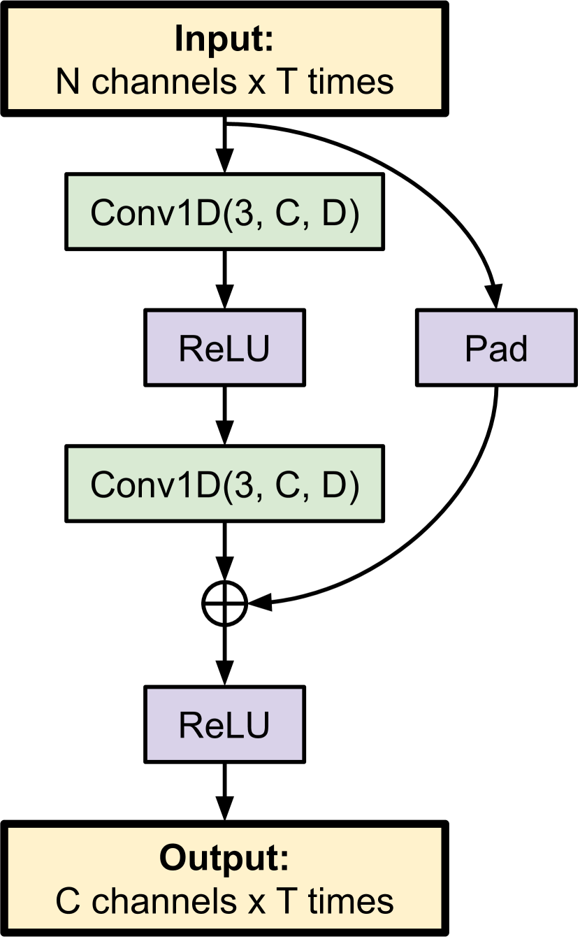
We implement the encoder using residual blocks with convolutional layers (He et al., 2016). Each block has two convolutional layers with a kernel size of 3, and we use ReLU activation functions. A schematic of each block is shown in Figure 2. We chain a series of seven these blocks together with increasing dilation sizes so that after all seven blocks the receptive field of the network contains the full light curve. In a traditional VAE, the posteriors of the latent variables would be predicted using fully connected layers. While such a network should be theoretically capable of representing the encoding functions for our model, in practice, we find that these networks are very unstable and difficult to train. To address this challenge, we add custom layers that are aware of the symmetries in our data to predict the explicit latent variables.

Figure 2: Architecture of the residual blocks used for the encoder of our model. Each block takes as input a 2D array consisting of $N$ channels at $T$ times. Two one-dimensional convolutional layers are applied along the time dimension with a kernel size of 3 and a dilation of $D$ elements. The input is then padded with zeros in the channel dimension and added with the output of the second convolutional layer to produce a 2D output with $C$ channels at $T$ times. We label this block as “ResidualBlock(D, C)”.

3.6 A Time-Invariant Encoder

The main challenge for convergence is computing the reference time $t_{0}$ for a light curve. At the start of training, the decoder will not be producing functions that look light light curves, so the gradient of the loss function with respect to $t_{0}$ will not be meaningful and the training will progress very slowly if at all. We address this by constructing a novel neural network architecture that is mathematically invariant to time translation.

The encoder predicts the hyperparameters $\mu$ and $\sigma^{2}$ describing the posterior distributions over the latent variables in our model. To predict the mean reference time $\mu_{t_{0}}$, we require our encoder to be a time-equivariant function, i.e. a function $f(t)$ that satisfies

$$f(t+\Delta t)=f(t)+\Delta t$$ (11)

For all of the other model hyperparameters, we require our encoder to be a time-invariant function, i.e. one that satisfies:

$$f(t+\Delta t)=f(t)$$ (12)

Convolutional layers on their own are equivariant: if the input to a convolutional layer is shifted, the output is identical but shifted by the same amount as the input. By applying a series of the residual blocks shown in Figure 2 without applying any pooling operations, we obtain an output that is mathematically equivariant to any shift in the input light curve by an integer number of days. The output of this layer is a two-dimensional array that has a length that is identical to the length of the input light curve (in our case 300 days) and 200 channels.

To produce a time-invariant function, we throw away all of the time information by applying a global max-pooling layer to this array. This operation involves taking the maximum value of the array over the time dimension to collapse it in the time dimension and produce a one-dimensional array with 200 channels. We use fully-connected layers over the collapsed array to predict all of the hyperparameters $\mu$ and $\sigma^{2}$ describing the posterior distributions over the latent variables in our model except for the mean reference time $\mu_{t_{0}}$. This procedure is mathematically invariant to any shift in time of the input light curves by an integer number of days.

To product a time-equivariant function, we begin with the previously-discussed (300 days) $\times$ (200 channels) array that was output from the residual blocks. We use a fully-connected layer applied to each bin in the time dimension individually to collapse the channel dimension and obtain a one-dimensional vector $v$ with a single value for each of the 300 time bins. We then apply a softmax transformation to this vector to obtain a 300-dimensional vector that sums to one. The entries in this vector can be thought of as weights for whether $\mu_{t_{0}}$ appears in a specific bin. We predict the value of $\mu_{t_{0}}$ by taking the dot product of this vector with the index of each element in the vector (i.e. a vector of increasing integers from 1 to 300).

$$\mu_{t_{0}}=\text{SoftMax}[v]\times\text{Index}[v]$$ (13)

Mathematically, if the input light curve is shifted by some integer number of days, then this function outputs a value for $\mu_{t_{0}}$ that is incremented by the same number of days as desired. We call this layer a “time-indexing layer”. By combining the time-indexing layer with the global max-pooling layer, we produce an encoder that is mathematically invariant to a translation in the input of any integer number of days with appropriate transformations for all of the latent variables. Note that we do not force the reference time to correspond with any specific feature of the light curve other than having a weak prior on the time of maximum light. We allow the model to automatically determine a relevant definition of reference time on its own.

3.7 Marginalizing Over the Amplitude

With the time-indexing layer the model is able to converge and give reasonable predictions. However, we find empirically that it is challenging for the model to predict the amplitude $A$. The amplitude corresponds to an overall scaling of the model, and is degenerate with a global scale of all of the outputs. We find that we can significantly improve the convergence of the model by modifying the architecture to marginalize over the amplitude rather than have it as an explicit parameter. To do this, note that given all of the other latent parameters $\bm{s}^{\prime}$, we can analytically evaluate the conditional posterior distribution of $A$ as:

$$p(A|\bm{s}^{\prime},\bm{y})=\frac{p(\bm{y}|\bm{s}^{\prime},A)p(A|\bm{s}^{\prime})}{p(\bm{y}|\bm{s}^{\prime})}$$ (14)

Here $p(\bm{y}|\bm{s}^{\prime})$ is a constant that does not depend on $A$. Assuming a Jeffreys (flat) prior for $p(A|\bm{s}^{\prime})$, this becomes:

$$p(A|\bm{s}^{\prime},\bm{y}) \propto p(\bm{y}|\bm{s}^{\prime},A)$$ (15)

$$\propto\prod\exp\left(-\frac{(\bm{y}-A\cdot d_{\bm{\theta}}(\bm{s}^{\prime},A=1))^{2}}{2\sigma_{\bm{y}}^{2}}\right)$$ (16)

$$=\frac{1}{\sqrt{2\pi\sigma_{A}^{2}}}\exp\left(-\frac{(A-\mu_{A})^{2}}{2\sigma_{A}^{2}}\right)$$ (17)

where:

$$\sigma_{A}^{2} =\frac{1}{\sum d_{\bm{\theta}}(\bm{s}^{\prime},A=1)^{2}/\sigma_{\bm{y}}^{2}}$$ (18)

$$\mu_{A} =\frac{\sum\bm{y}\cdot d_{\bm{\theta}}(\bm{s}^{\prime},A=1)/\sigma_{\bm{y}}^{2}}{\sum d_{\bm{\theta}}(\bm{s}^{\prime},A=1)^{2}/\sigma_{\bm{y}}^{2}}$$ (19)

We can then evaluate the log-likelihood $\log p_{\bm{\theta}}(\bm{y}|\bm{s}^{\prime})$ necessary for the VAE loss function in Equation 1 as:

$$\log p_{\bm{\theta}}(\bm{y}|\bm{s}^{\prime}) =\int dA\cdot p(\bm{y}|\bm{s}^{\prime},A)\cdot p(A|\bm{s}^{\prime})$$ (20)

$$=\int dA\cdot p(\bm{y}|\bm{s}^{\prime},A)+C$$ (21)

where $C$ is some arbitrary normalization constant that can be ignored because it will not affect the minimization. We estimate this integral numerically using importance sampling with $A$ drawn from its posterior distribution shown in Equation 17. As is typically done when training deep learning models, while training we use a single sample for our numerical estimate of the integral.

With this procedure, we analytically marginalize over the amplitude $A$ and it is no longer an explicit parameter of our model. The Jeffreys prior that we impose on $p(A|\bm{s}^{\prime})$ is improper, which means that we are not learning a generative model for the amplitude. This is not a problem for most science applications as discussed in Section 6.4, and a similar approach is taken for most generative models of SNe Ia (e.g. SALT2; Guy et al., 2007). We find that this model that marginalizes over the amplitude is much easier to train than a model where the amplitude is an explicit parameter.

3.8 Regularization of the Spectra

As discussed in Section 3.3, we are training our model to predict the full spectra of transients. We are only training using photometry in this work, which means that we are effectively performing a deconvolution. As a result, the high-frequency components of the spectra will not be well-constrained. To prevent the model from adding high-frequency noise to the spectra, we add a regularization term to our loss function following a procedure similar to the one used by Crenshaw & Connolly (2020) for estimating galaxy spectra from photometry. Given the set of wavelength bins with index $n$, we apply a penalty on the flux difference between adjacent bins given by:

$$\eta\sum_{i}\left(\frac{d_{\text{int},\bm{\theta},n}(\bm{t},\bm{s}_{i})-d_{\text{int},\bm{\theta},n+1}(\bm{t},\bm{s}_{i})}{d_{\text{int},\bm{\theta},n}(\bm{t},\bm{s}_{i})+d_{\text{int},\bm{\theta},n+1}(\bm{t},\bm{s}_{i})}\right)^{2}$$ (22)

Here $\eta$ is a tunable parameter that can be adjusted to determine the strength of the regularization. We apply this penalty to the full spectra that are predicted at every time where we have an observation. We find empirically that a value of $\eta=0.001$ results in a reasonable balance between reducing noise and oversmoothing the spectrum. We find that this regularization term contributes only $\sim$0.01% to the loss function at the end of training for both of the datasets that we consider.

3.9 Augmentation

As shown in Boone (2019), augmentation can be used to generate a wide range of different light curves from observations of a single transient. When training our model, we apply a series of different random transformations to our data. These transformations are all applied independently, and we choose different transformations in each epoch.

• Shift the observations by a constant offset sampled from a Normal[0, 20 days] distribution.

• Scale the observations by a constant factor sampled from a Lognormal[0, 0.5] distribution.

• Drop observations randomly, with the fraction to drop sampled from a Uniform[0, 0.5] distribution.

• With probability 50%, add noise to the observations with a standard deviation sampled from a Lognormal[-4, 1] distribution.

These transformations produce a wide range of light curves, with some resembling the original light curves and others at much lower signal-to-noises with significantly fewer observations. In contrast to Boone (2019), we do not attempt to augment our light curves in redshift as that cannot be done without making assumptions about the shape of the spectrum. We also do not attempt to reproduce the observational properties of the instrument. Instead, we simply attempt to cover a wide range of signal-to-noises ranging from the original values to signal-to-noises well-below the detection threshold.

3.10 The ParSNIP model

We combine all of the different elements described in this Section to build a hybrid physics-VAE model that can describe transient light curves. We call this model “ParSNIP” (Parametrization of SuperNova Intrinsic Properties). A schematic of the full ParSNIP architecture is shown in Figure 3.

Figure 3: Architecture of the ParSNIP model.

We implemented this model in PyTorch (Paszke et al., 2019). We fit the model separately to the PS1 and PLAsTiCC datasets of transient light curves described in Section 2 using the Adam optimizer (Kingma & Ba, 2015) with a learning rate of $10^{-3}$ and batch sizes of $128$. We use the ReduceLROnPlateau feature in PyTorch to scale the learning rate by a factor of $0.5$ whenever the optimizer fails to reduce the loss function after 10 epochs, and we train until the learning rate is decreased to below $10^{-5}$. This training procedure takes approximately 300 epochs. The computation times and requirements for both training and inference are discussed in Section 6.1.

3.11 Hyperparameters

Our model has many different hyperparameters that can be tuned, including the architecture of the network and the parameters of the optimizer. We trained 56 models on the PS1 dataset using a wide range of different hyperparameter values. We trained on 90% of the dataset, and kept 10% back for validation. We find that the model is not highly sensitive to most hyperparameters other than the learning rate, with the loss function typically varying by $<5\%$. The results are consistent for the training and validation sets. When the model performs similarly well on two different configurations, we choose the one that is more computationally efficient. We show the range of hyperparameter values that we considered along with the optimal values from our tests in Table 1.

Table 1: Hyperparameter optimization for the ParSNIP model. We show the range of values considered for each hyperparameter along with the value that resulted in the model with the smallest loss function in bold. When arrays are given, each element in the array refers to the hyperparameter value for a different block in the architecture. The optimal configuration is shown in Figure 3.

Hyperparameter	Value
Batch size	16, 32, 64, 128, 256, 512
Learning rate	$10^{-4}$, $2\times 10^{-4}$, $5\times 10^{-4}$, $\bm{10^{-3}}$, $2\times 10^{-3}$, $5\times 10^{-3}$, $10^{-2}$
Scheduler factor	0.1, 0.2, 0.5
Encoder convolutional block types	Conv1d, ResidualBlock
Encoder convolutional block widths	[20, 40, 60, 80, 100, 100, 100]
	[40, 80, 120, 160, 200, 200, 200]
	[32, 64, 128, 128, 128, 128, 128]
	[32, 64, 128, 256, 256, 256, 256]
	[32, 64, 128, 256, 512, 512, 512]
Encoder fully connected block sizes	100, 128, 200, 256, 400, 512
Decoder architecture	[100]
	[50, 100]
	[100, 200]
	[40, 80, 160]
	[64, 128, 256]
	[32, 64, 128, 256]

3.12 Dimensionality of the Intrinsic Latent Representation

Another important hyperparameter is the dimensionality of the intrinsic latent representation. We trained the ParSNIP model with varying numbers of intrinsic dimensions and with all of the other hyperparameters kept at their optimal values shown in Table 1. For each model, we evaluated the VAE loss function shown in Equation 1 on both the training and validation subsets of the PS1 dataset. The results of this procedure are shown in Figure 4.

Figure 4: VAE loss function for different dimensionalities of the intrinsic latent representation. For each number of dimensions we train three models (shown as black dots), and we shown the mean value of the loss function across all three models with colored markers. Beyond three dimensions we see little improvement in the VAE loss function.

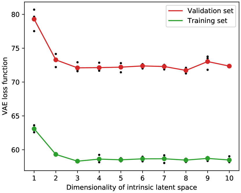
We find that the loss function improves when increasing the dimensionality up to three for both the training and validation sets, but there is little benefit from adding more dimensions beyond three. For models with large numbers of dimensions, we find that most of the dimensions are not used by the VAE, and it simply outputs uninformative $\mathcal{N}(\bm{0},\bm{1})$ posteriors for all of the transients in some dimensions. We choose to use a three-dimensional model for the rest of our experiments.

4 Model Performance

4.1 Reproducing Light Curves

To study how well our model can reproduce light curves, we trained the ParSNIP model on 90% of the light curves in the PS1 dataset described in Section 2 with a randomly selected 10% of the light curves held out for validation. We show examples of the models for different light curves in the validation subset in Figure 5. We find that the ParSNIP model is able to generalize well on the PS1 dataset with accurate models for the vast majority of transients.

Figure 5: Examples of out-of-sample predictions of the ParSNIP model on the validation subset of the PS1 dataset. These light curves were not included in the dataset that was used to train the model. Each panel shows the predictions for a different light curve. The observations are shown as individual points with their uncertainties, and the different colors correspond to the different bands as shown in the legend. The mean model predictions are shown as a solid line, and the 1-sigma uncertainties from varying the VAE latent parameters are shown with shaded contours.

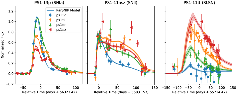
We calculated the model residuals for all of the observations in our dataset. For the PS1 training set, we find that the model residuals are consistent with the statistical uncertainties which suggests that may we have somewhat overfit the training set. For the validation set, we find that the distribution of the residuals has a tight core with a dispersion of $\sim$0.06 mag when statistical uncertainties are taken into account. We do however see large residuals for some light curves, particularly ones of transient types that are not well represented in the training set. For observations with a statistical uncertainty of less that 0.05 mag, we find that 94% of observations have residuals of less than 0.2 mag, and $99.2$% of observations have residuals of less than 0.5 mag.

We performed the same comparison for a version of the ParSNIP model trained on 90% of the light curves in the PLAsTiCC dataset. In this case, we find that the model residuals have a tight core with a dispersion of $\sim$0.04 mag when statistical uncertainties are taken into account. For observations with a statistical uncertainty of less than 0.05 mag, we find that 97% of observations have residuals of less than 0.2 mag and $99.7$% of observations have residuals of less than 0.5 mag, with no major differences between the training and validation sets. The PLAsTiCC dataset was simulated and the subset that we used to train the model contains more than 100 times as many transients as the PS1 dataset which likely explains the difference in training/validation performance between the PS1 and PLAsTiCC datasets. Overall, we find that the ParSNIP model is able to produce good models for the vast majority of the light curves in both datasets.

4.2 The ParSNIP Intrinsic Latent Space

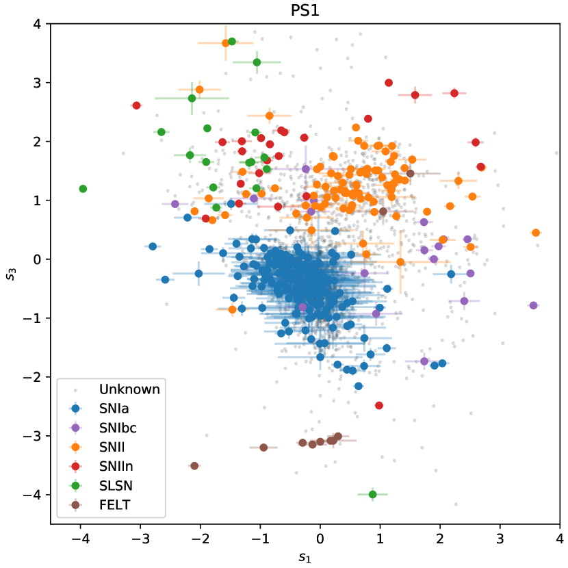
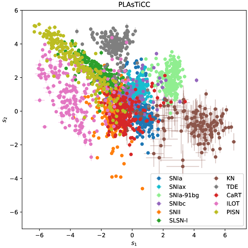
As described in Section 3.3, the ParSNIP model learns a three dimensional intrinsic latent space $\bm{s}_{i}$ describing the intrinsic diversity of transients. To study the structure of the learned latent spaces, we look at where transients with known labels are located in the latent space for both of our datasets. The results of this procedure are shown in Figure 6. Most of the different transient types are well separated despite the fact that the type labels were not used when training the ParSNIP model.

Figure 6: Visualization of the intrinsic latent spaces learned when trained on the PS1 (left panel) and PLAsTiCC (right panel) datasets. We show two of the $\bm{s}_{i}$ latent variables for each transient in the dataset, and we color each transient by its type if known. We limit this plot to show a maximum of 200 transients for each type to highlight rarer types. Despite the fact that the types were not used when training the ParSNIP model, the model groups transients of the same type at similar locations in the latent space. Note that these plots show only two dimensions of the intrinsic latent space: each light curve also has measurements of another $\bm{s}_{i}$ latent variable, color, and amplitude.

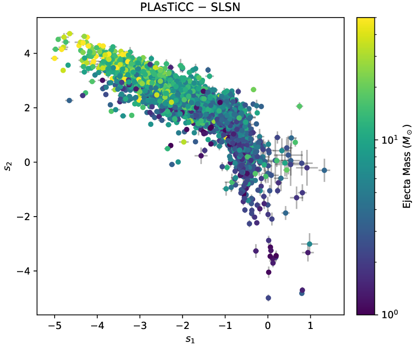
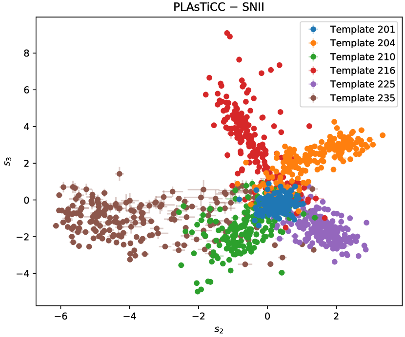
For transients of the same type, we find that differences in the ParSNIP intrinsic latent variables $\bm{s}_{i}$ correspond to differences in the intrinsic properties of the transients. This can easily be see using the PLAsTiCC dataset where all of the parameters that were used for simulating each light curve are known. In the left panel of Figure 7, we show that the ParSNIP latent space of superluminous supernovae is capturing the variation in ejecta mass that went into the simulations. The SNe II were simulated using a small number of discrete templates, and we show where light curves simulated from some of these templates are located in the latent space in the right panel of Figure 7. The ParSNIP model identifies these discrete templates and clusters light curves simulated from each of them in the latent space.

Figure 7: Examples of diversity of the ParSNIP intrinsic representations for transients of the same type in the PLAsTiCC dataset. Left panel: The variation of ParSNIP $s_{1}$ and $s_{2}$ latent variables for superluminous supernovae is explained by differences in the ejecta mass parameter (shown in color) that went into the simulations. Right panel: Some of the Type II supernovae in the PLAsTiCC dataset were simulated using discrete templates. We show the $s_{2}$ and $s_{3}$ latent variables for light curves simulated from six of these templates, and find that the light curves simulated from each template cluster at similar locations in the ParSNIP intrinsic latent space.

As discussed in Section 3, the ParSNIP model was constructed to produce an intrinsic latent space that is invariant to how the light curve was observed. As expected, we find that well-measured light curves simulated with similar parameters are embedded at very similar locations in the intrinsic latent space even when those light curves are observed at different redshifts, with different brightnesses, or with different amounts of host galaxy dust. There are no major correlations between any of these properties of the observations and the intrinsic latent variables $\bm{s}_{i}$.

To demonstrate the invariance of the ParSNIP model to redshift, we show the recovered intrinsic latent space for the PLAsTiCC dataset in different redshift slices in Figure 8. We find that the recovered latent space is almost identical in all of the different redshift slices. There are minor differences across redshift bins for some of the transient types. For example, the SNe II have a much broader distribution in the lower redshift bins compared to the higher redshift bins. These differences are due to Malmquist bias rather than a limitation of the ParSNIP model. At low redshifts nearly all SNe II are detected, but at high redshifts only the SNe II that are intrinsically very bright are detected. For the PLAsTiCC dataset, this means that at low redshifts the SNe II come from a wide range of templates giving a wide distribution in latent space, but at high redshifts the majority of the observed SNe II come from a single template (number 235) and are clustered tightly in the latent space.

Figure 8: Visualization of the intrinsic latent space learned for the PLAsTiCC dataset in different redshift ranges. The redshift range of each panel is shown above the panel. In each panel, we show the $s_{1}$ and $s_{2}$ latent variables for 200 transients of each type, and we color each point by its type. The ParSNIP model was constructed to produce an intrinsic latent space that is invariant to observing conditions such as redshift, and we find that the latent spaces are nearly identical in each of the different redshift slices. The slight differences such as the narrowing of the SNe II distribution at high redshifts are due to Malmquist bias rather than a limitation of the ParSNIP model. Note that some transient types have a limited redshift range in the PLAsTiCC simulations so they do not appear in some of the redshift slices.

4.3 Comparison with SALT2

The SALT2 model (Guy et al., 2007) is commonly used to model the light curves of SNe Ia. This model is a linear model with one parameter $x_{1}$ describing the variability in the observed widths of SN Ia light curves, and a second parameter $c$ describing the differences in color (which will capture host galaxy dust). As described in Section 3.3, the ParSNIP model is effectively a generalization of the SALT2 model. In this subsection, we compare the performance of both of these models for SNe Ia. Note that the PLAsTiCC SN Ia light curves were simulated using SALT2. For a fair comparison, we only consider the version of the ParSNIP model that was trained on real PS1 light curves and is thus independent of SALT2.

We investigated whether the latent space that the ParSNIP model learns for SNe Ia captures the $x_{1}$ and $c$ parameters of the SALT2 model. To do this, we fit the SALT2 model to all of the light curves that were labeled as SNe Ia in the PS1 dataset and compared the results with the ParSNIP model on the same subset of light curves. We limited our comparison to light curves that are well-fit by SALT2, which we define as having a fit that converges, a best-fit SALT2 $x_{1}$ parameter between $-5$ and $+5$, an uncertainty on $x_{1}$ of less than 0.5, an uncertainty on SALT2 $c$ of less than 0.1, and at least one observation before maximum light.

The ordering of the intrinsic latent variables $\bm{s}_{i}$ in the ParSNIP model is arbitrary. To effectively compare our parameterization of the intrinsic diversity to $x_{1}$, we solve for the linear combination of the ParSNIP latent variables $\bm{s}_{i}$ that best models $x_{1}$:

$$x_{1}^{\text{ParSNIP}}=\gamma_{0}+\sum_{n}\gamma_{n}s_{i,n}$$ (23)

We solve for the coefficients $\gamma_{n}$ that minimize the sum of squared differences between $x_{1}^{\text{ParSNIP}}$ and $x_{1}$. Note that we do not include measurement uncertainties in this procedure because both the SALT2 and ParSNIP models were fit to the same observations and the uncertainties on the $\bm{s}_{i}$ and $x_{1}$ latent variables are likely very highly correlated. The results of this procedure are shown in the left panel of Figure 9.

Figure 9: Reproducing the SALT2 model parameters from the ParSNIP latent space. Left panel: SALT2 $x_{1}$ as a function of the best-fit linear combination of the ParSNIP intrinsic latent variables $s_{i}$. Right panel: SALT2 color as a function of the ParSNIP color with a constant offset. The one-to-one line is shown in blue in both plots. We are able to recover both SALT2 $x1$ and $c$ from the ParSNIP latent space with high accuracy.

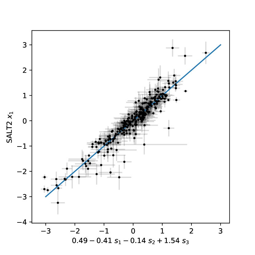
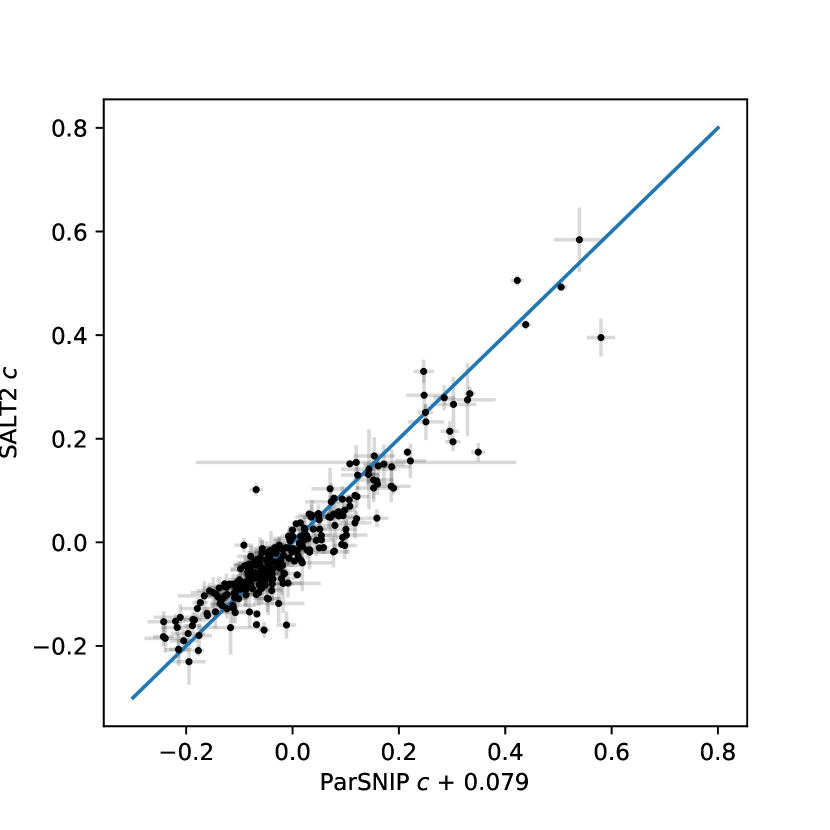
In the right panel of Figure 9, we show the SALT2 $c$ parameter in terms of the ParSNIP $c$ parameter. We include a constant offset in this comparison given by the difference in the median colors between both datasets to account for different arbitrary zeropoints. We are able to accurately predict the SALT2 $x_{1}$ and $c$ parameters from the ParSNIP latent space for all of these SNe Ia, with 88% and 89% of the variance explained respectively. The residuals from the predictions for $x_{1}$ have an NMAD of 0.24 and a standard deviation of 0.34. The differences between the ParSNIP $c$ and SALT2 $c$ values have an NMAD of 0.037 mag and a standard deviation of 0.044 mag. The differences between the ParSNIP $c$ and SALT2 $c$ values are highly correlated with the $s_{3}$ parameter ($\rho$=0.64) which simply reflects the fact that the color zeropoint is arbitrary and can vary across the parameter space. Our prediction of SALT $c$ could be further improved if this were taken into account. To summarize, given the location of an SN Ia in the ParSNIP latent space we are able to accurately predict its SALT2 parameters. This implies that the ParSNIP latent space contains all of the information that is captured by the SALT2 parameterization of SNe Ia.

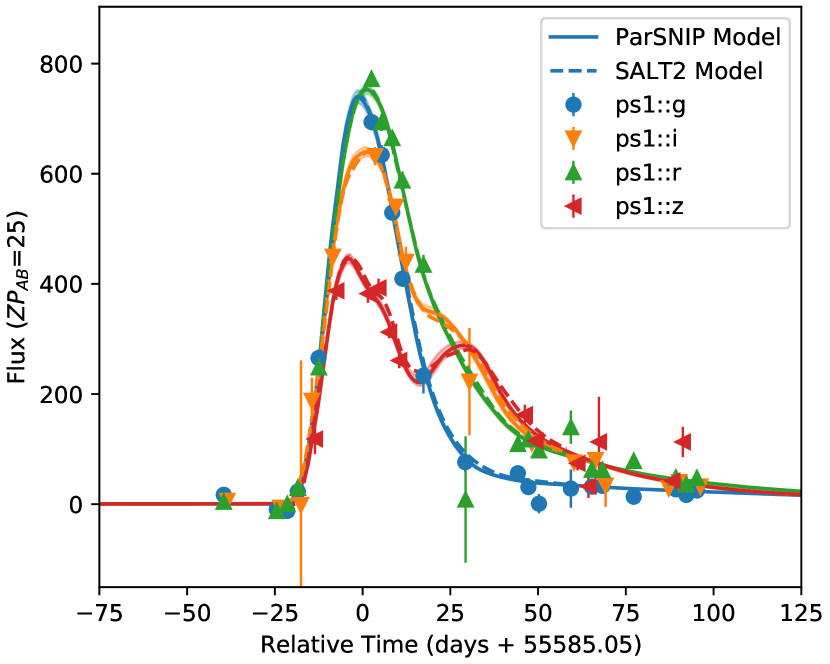
We compared how well the SALT2 and ParSNIP models are able to reproduce light curves. An example of the light curve fits of both models to PS1-11bk is shown in the top panel of Figure 10. The quality of the light curve fits are comparable. For the training set (validation set), we find a median reduced $\chi^{2}$ of 1.42 (1.68) for ParSNIP fits to SNe Ia and 1.40 (1.21) for SALT2 fits. Note that for SALT2 we found the exact maximum likelihood values of the model parameters by fitting the model to the light curves. For the ParSNIP model, we instead used the encoder to approximate the maximum-a-posteriori values of the model parameters. All of the ParSNIP reduced $\chi^{2}$ values would decrease if a full fit were performed to find the true maximum likelihood values of the model parameters. Nevertheless, we find that the ParSNIP model is achieving comparable reconstruction performance to the SALT2 model despite being trained on a much lower quality dataset.

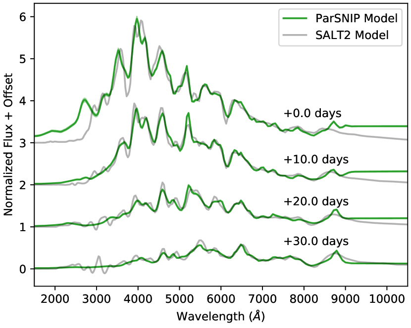
Both SALT2 and ParSNIP predict the full spectral time series of the light curves that they fit. We compare the predicted spectra for PS1-11bk at a range of different times in the lower panel of Figure 10. The SALT2 model was trained using spectra of a large number of SNe Ia and is known to provide a good description of the spectra of SNe Ia. In contrast, the ParSNIP model was trained using only photometric observations. Nevertheless, the ParSNIP model accurately reproduces all of the major spectral features of SNe Ia as seen in the SALT2 model. The ParSNIP model does have some non-physical behavior at UV and IR wavelengths (as does SALT2) where the PS1 bandpasses have limited coverage. This could be improved by including additional followup observations in the training. We discuss this further in Section 6.7. We stress that the ParSNIP model was able to learn the spectrum of an SN Ia by effectively deconvolving photometric observations of SNe Ia at a wide range of different redshifts, and no spectra were included in the training dataset.

Figure 10: Comparison of the SALT2 and ParSNIP models for the SN Ia PS1-11bk. Top panel: Comparison of the light curves. The ParSNIP model is shown with solid lines, and the SALT2 model is shown with a dashed line. Bottom panel: Comparison of the spectra predicted by both models at a range of different times. We find good agreement between the SALT2 and ParSNIP models other than in the UV and IR regions that are not covered by many observations.

4.4 Models of Other Kinds of Transients

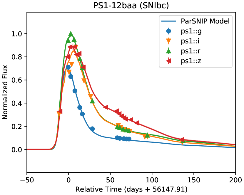
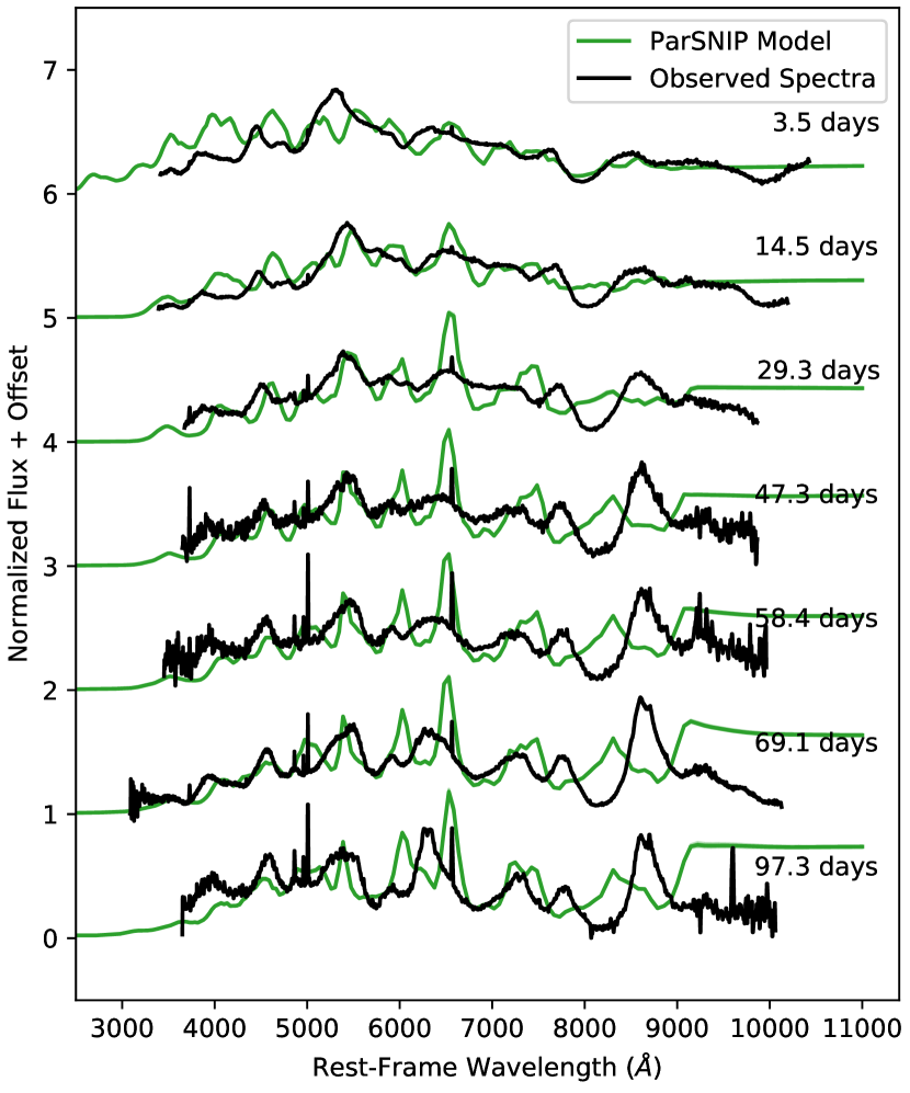
While empirical models such as SALT2 have been previously developed for SNe Ia, models of other kinds of transients are typically much more primitive due to the lack of spectroscopic observations and more complex variability. Our techniques produce a generative model for the spectral time series of all of these transients. To evaluate the performance of these models, we compare the spectral time series predicted by ParSNIP to observed spectra for two different core-collapse supernovae: PS1-12cht, a Type IIn supernova and PS1-12baa, a peculiar Type Ic supernova. We retrieved spectra for these two supernovae from the Open Supernova Catalog (Guillochon et al., 2017). Both of these supernovae are from classes that are not well-sampled in the PS1 dataset, so we show results from a run where these supernovae were included in the training of the ParSNIP model.

Figure 11: Comparison of the ParSNIP model to observed spectra of core-collapse supernovae. The left two panels show the model and data for PS1-12cht, a Type IIn supernova, and the right two panels show the model and data for PS1-12baa, a peculiar Type Ic supernova. The top two panels show the observed PS1 photometry and the ParSNIP model fit to that photometry. The bottom two panels show observed spectra for each of these supernovae from PESSTO (Smartt et al., 2015) and LOSS (Shivvers et al., 2019) respectively along with spectra from the ParSNIP model evaluated at the same phases. We normalize all of the spectra to the flux at 6000Å. We find that the broad structure of the ParSNIP predicted spectra agree well with the observed spectra despite the fact that the ParSNIP model was only trained using photometry.

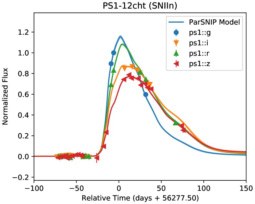
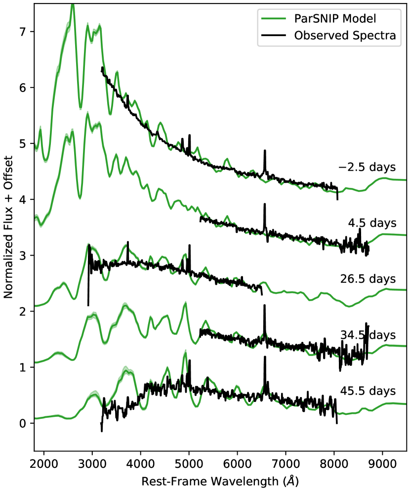
In the left panel of Figure 11, we show the light curve and spectra of PS1-12cht, a Type IIn supernova. These spectra were obtained by the PESSTO collaboration (Smartt et al., 2015) and are relatively featureless. We find that the ParSNIP model produces good predictions of the overall shape of the spectra and the photometry, although we do see some ringing of the spectra at bluer wavelengths.

In the right panel of Figure 11, we show the light curve and spectra of PS1-12baa, a peculiar Type Ic supernova. These spectra were obtained by the LOSS collaboration (Shivvers et al., 2019). The spectra of this supernova show many different emission lines, especially at later times. The ParSNIP model predictions agree well with the observed spectra at early times and reproduce most of the observed spectral features. At later times, we find that the ParSNIP model is able to predict the broad structure of the spectrum, but it struggles to predict the exact locations and widths of all of the emission lines.

This is not surprising: the ParSNIP model was only trained on photometry, so the estimates of the spectra come from effectively deconvolving the photometry of many transients at different redshifts. PS1-12baa is a peculiar Type Ic supernova, and there are very few examples of similar supernovae in the PS1 dataset. The deconvolved spectra are therefore not very well constrained. This could be addressed by training on a larger dataset, such as the one that the Rubin Observatory will produce, or by including spectra or additional followup observations in the training process. These options are discussed in Section 6.7.

4.5 Comparison with Simulations

The PLAsTiCC dataset was simulated, so we can compare the spectra predicted by the ParSNIP model directly to those that were used in the simulation. The result of this procedure is shown for well-measured light curves of a range of different types of transients in Figure 12. Some classes, such as Type II supernovae, were simulated using several different models with very different spectral properties. We find that the ParSNIP model is able to identify the different models and recover the underlying spectral time series for each of them.

Figure 12: Comparison of the spectra predicted by the ParSNIP model to the true spectra in the PLAsTiCC simulations. Each panel shows the simulated spectra for a given transient in grey at a range of different times. The spectra predicted by the ParSNIP model for that transient are shown in green. The titles of each panel indicate the type of transient and model that was used for the simulation. We find that the ParSNIP model is able to accurately recover the spectral time series of all of these different kinds of transients despite only being trained on photometry.

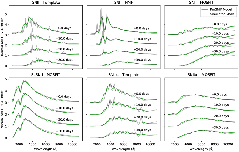
The spectra that are recovered by the ParSNIP model tend to be overly smooth compared to the input simulations. This is primarily due to the fact that we are learning the spectra by deconvolving photometry. The regularization term described in Section 3.8 can be adjusted to recover more of the spectral features, but this comes at the cost of introducing additional noise into the model. In practice, we find that they choice of regularization term has little impact on the final photometry because all of the high frequency information is lost after the convolution with the bandpass.

5 Applications

There are many different applications for a generative model of all transient light curves. We discuss three of them in this section. In Section 5.1, we show how the ParSNIP model can be used to perform photometric classification even with heavily biased training sets. In Section 5.4, we demonstrate a novel method of searching for new kinds of transients. In Section 5.5, we show how the ParSNIP model can be used to estimate cosmological distances to SNe Ia.

5.1 Photometric Classification

Upcoming surveys such as the LSST with the Rubin Observatory will obtain photometric observations of millions of transients, but will only have the spectroscopic resources to obtain spectroscopy of and label a small fraction of these transients. Traditional classification techniques only use this small dataset of labeled transients for training (e.g. Lochner et al. (2016); Boone (2019)). In contrast, autoencoder-based methods can learn a low-dimensional representation from the much larger dataset of both labeled and unlabeled transients. This representation is a set of very informative features which can be used to train a photometric classifier on the small labeled dataset. This approach has previously been demonstrated in Pasquet et al. (2019) and Villar et al. (2020).

The main advantage of ParSNIP over previous autoencoders is that the representation that it learns was constructed to disentangle intrinsic properties of transients from properties describing how transients were observed. In particular, the intrinsic representation is disentangled from redshift. The labeled training sets tend to be heavily biased towards low-redshift transients, so redshift is not a good feature to use for classification. Pasquet et al. (2019) attempted to construct a similar representation using a contrastive loss function that adds a penalty when transients with the same label have very different representations. This technique is effective, but requires a representative sample of labeled high redshift transients that is often not available. In contrast, ParSNIP can generate such a representation with only the unlabeled dataset because it is a full generative model.

To perform photometric classification with ParSNIP, we first augment each light curve in the training set 100 times following the procedure in Section 3.9. Note that we do not perform redshift augmentation as in Boone (2019), we only use augmentation to obtain light curves at a wide range of signal-to-noises and observing conditions. We then perform inference using the ParSNIP model to estimate the latent representations for all of the transients in the augmented training set. We convert the amplitude measured by the ParSNIP model to a pseudo-luminosity $L$ using the cosmological parameters from Planck Collaboration et al. (2020) with the following formula:

$$L=-2.5\log_{10}(A)-\mu_{\text{Planck20}}(z)+25$$ (24)

The offset of 25 comes from the fact that the input fluxes for both the ParSNIP and PLAsTiCC datsets were measured on the AB system with a zeropoint of 25. We refer to $L$ as a pseudo-luminosity because it contains an arbitrary offset from the unknown zeropoint of the ParSNIP model. This offset will be identical for all light curves with the same intrinsic representation. We use the full ParSNIP representation as the features for our classifier, consisting of the intrinsic latent variables $s_{1}$, $s_{2}$, $s_{3}$, the pseudo-luminosity $L$, and the color $c$. We also include the predicted uncertainties on all of these measurements and the uncertainty on the reference time for a total of eleven features. We do not include redshift as an explicit feature as the redshift distributions of the labeled and unlabeled datasets tend to be very different, although the redshift is used to calculate the luminosity.

We train a gradient boosted decision tree on these features using the lightgbm package (Ke et al., 2017). When training this classifier, we weight each transient in the training set so that the sum of weights for each label is equal and so that the average weight across all transients is one. We use the default hyperparameter values from lightgbm with a multi_logloss objective function, except that we set the min_child_weight parameter to 1000 to avoid overfitting the augmented light curves. We train the classifiers with 10-fold cross validation: we train each classifier on 90% of the data and evaluate the model on the remaining 10%. We repeat this procedure ten times to obtain ten separate classifiers and out-of-sample predictions for all of the transients in the training set. To avoid data leakage, we ensure that all augmentations of the same light curve are in the same fold for this procedure. For the unlabeled dataset, we generate predictions by averaging over the outputs of all of the classifiers.

5.2 Photometric Classification on the PS1 Dataset

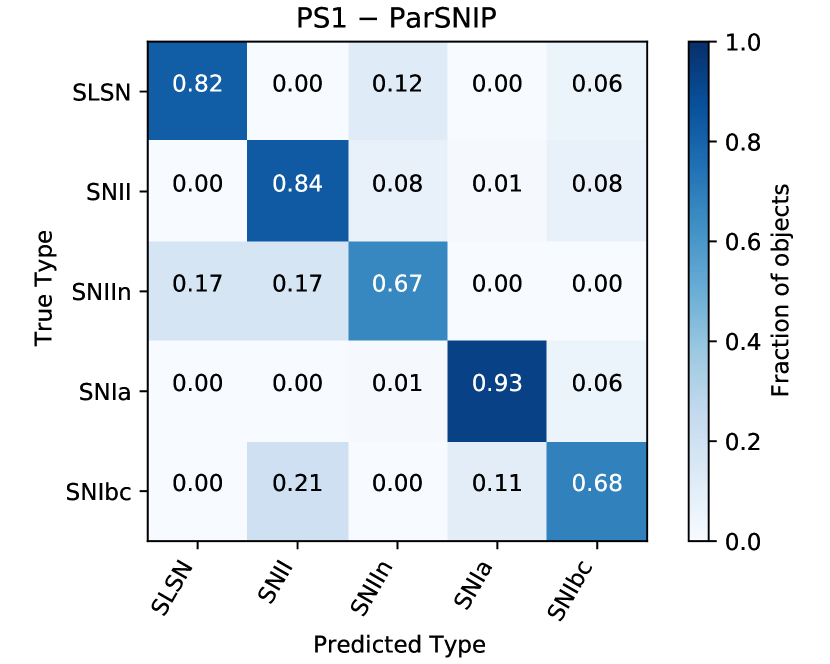
For the PS1 dataset, we only have labels for a subset of 557 transients. We predict the labels for each of these transients using 10-fold cross-validation. In Figure 13, we show a confusion matrix for this dataset. Each row of the confusion matrix shows what fraction of the transients of a given type are assigned to each label by the classifier. We find that the ParSNIP model is able to accurately classify all of the different types of transients in this dataset, with 63% to 92% of the transients of each type being correctly identified in a five-way classification.

Our results are a significant improvement from both the SuperRAENN (Villar et al., 2020) and Superphot (Hosseinzadeh et al., 2020) models that have previously been applied to this dataset. We achieve an overall accuracy of 89% for the five-way classification compared to 87% for SuperRAENN on the same dataset. For the metric of the“macro-average completeness” defined in Villar et al. (2020) (the mean of the diagonal terms in the confusion matrix), we achieve a value of 79% with ParSNIP compared to 69% for both SuperRAENN and Superphot. For a two-way classification of SNe Ia compared to all other labels, we achieve a macro-averaged completeness of 96% compared to 92% for SuperRAENN. This implies that a sample of SNe Ia that was photometrically classified with ParSNIP would have $\sim$2 times less contamination than a sample classified with SuperRAENN.

These predictions were all made through cross-validation, so the classifiers were evaluated on datasets that have very similar properties to the datasets that they were trained on. The major advantage of ParSNIP over previous models is that its representation is invariant to symmetries such as redshift, and it is designed to perform well even when the training set differs significantly from the dataset that the classifier is applied to. We expect that the improvement in performance of ParSNIP over previous models such as SuperRAENN or Superphot will be even larger when applied to the non-representative datasets such as the ones that will be produced by the Rubin Observatory or the Rubin Space Telescope. Unfortunately it is impossible to test this performance on real data since we do not have access to the true labels for the higher redshift transients, although we can test it on simulations.

Figure 13: Confusion matrix for the cross-validated ParSNIP predictions on the PS1 dataset. Each entry shows the fraction of transients of the type labeled on the left side of the plot that are assigned the corresponding type labeled on the bottom of the plot.

5.3 Photometric Classification on the PLAsTiCC Dataset

The PLAsTiCC dataset is a simulation of the LSST light curve sample, and has a labeled training set that is highly nonrepresentative of the full dataset. We compare the performance of the ParSNIP model for classification of the PLAsTiCC light curves to the performance of the Avocado model (Boone, 2019) that was the best performing classifer in the PLAsTiCC challenge (Hložek et al., 2020). In the version of ParSNIP discussed in this work, we assume that we know the redshift of each transient but this information was not available in the original PLAsTiCC dataset. For a fair comparison, we retrained the Avocado classifier using the true redshifts instead of photometric redshifts. We show the confusion matrices for both the ParSNIP and Avocado classifiers in Figure 14.

Figure 14: Confusion matrices for the ParSNIP (left panel) and Avocado (right panel) predictions on the PLAsTiCC test set. Each entry shows the fraction of transients of the type labeled on the left side of the plot that are assigned the corresponding type labeled on the bottom of the plot. We find that the ParSNIP model has similar or better performance than the Avocado model for every kind of transient.

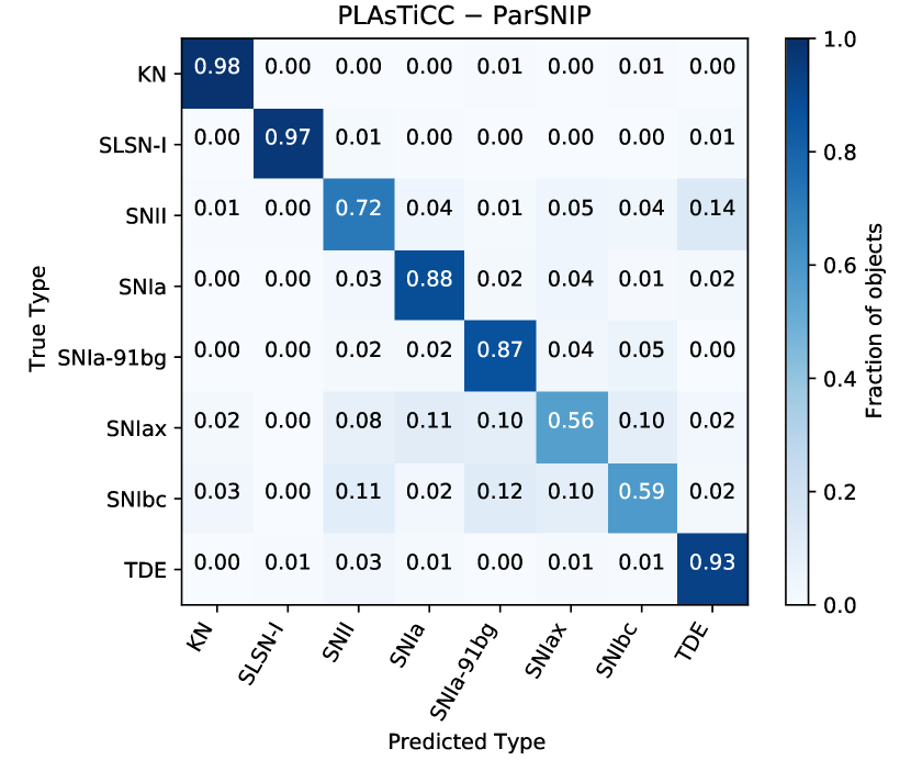
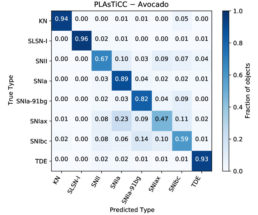
The ParSNIP model achieves similar or better performance than Avocado for each of the different kinds of transients. We evaluated the weighted log-loss metric developed for the PLAsTiCC challenge (Malz et al., 2019) limited to the subset of transient types used in this analysis. Avocado scores 0.599 on this metric while ParSNIP scores 0.535 which is a major improvement. To illustrate how this difference in performance will affect astrophysical analyses, we evaluated the receiver operating characteristic (ROC) curve for both of these classifiers for SNe Ia. This curve measures the true positive rate (the fraction of SNe Ia that are correctly classified as SNe Ia) as a function of the false positive rate (the fraction of non-SNe Ia that are misclassified as SNe Ia) for different thresholds of the classifier output. We show the ROC curve for both the ParSNIP and Avocado classifiers in Figure 15.

Figure 15: Receiver operating characteristic (ROC) curve for SN Ia classification on the PLAsTiCC dataset. The ParSNIP model (shown in blue) performs significantly better than the Avocado model (shown in orange), especially for thresholds corresponding to low false positive rates that are most interesting for supernova cosmology analyses.

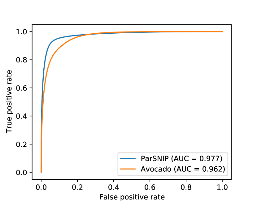
Measuring the Area Under the ROC Curve (AUC) (the integral of this curve), we find a value of 0.977 for the ParSNIP model compared to 0.962 for the Avocado model. The improvement of the ParSNIP model mainly comes from a major reduction in the false positive rate for true positive rates below $\sim 90\%$. For a true positive rate of 50%, the ParSNIP model has a false positive rate of only 0.44% which is 2.3 times smaller than the false positive rate of 1.04% for the Avocado model. We find similar results for any true positive rate below 0.9. This is of particular importance for cosmology analyses with SNe Ia where it is more important to have a clean dataset than include all transients that were discovered. A SN Ia cosmology analysis that uses the ParSNIP model for classification will have 2.3 times less contamination from other supernova types compared to an analysis that uses the Avocado model.

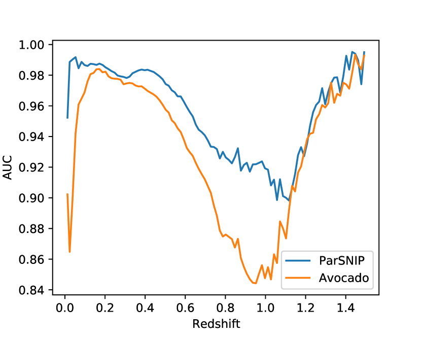
Finally, we evaluated the performance of both the ParSNIP and Avocado models as a function of redshift. We evaluated the AUC for classification of SNe Ia in 100 evenly-spaced redshift bins between redshifts of 0 and 1.5. The results for both the Avocado and ParSNIP models are shown in Figure 16. We find that the ParSNIP model is stable across different redshifts, and outperforms the Avocado model at all redshifts. Of particular note is the decrease in performance for the Avocado model at very low redshifts where we would expect to have very high signal-to-noise and well-measured light curves. The Avocado model attempts to augment the training dataset by simulating light curves at redshifts that are more representative of the full dataset, but struggles to produce good simulations of very low redshift transients because light curves at those redshifts are much higher signal-to-noise than most of the light curves in the training set. Fundamentally, the Avocado augmentation process must be heavily tuned for each dataset that it is applied to in order to minimize differences between the training and test sets.

In contrast, the ParSNIP model builds a redshift-independent representation of light curves from the full dataset, and is mostly agnostic to differences in the redshift distributions between the training and full datasets. Other than definitions of the bandpasses, there are no instrument-specific elements of the ParSNIP model. The same ParSNIP model was able to fit both the PLAsTiCC and PS1 datasets. We find that the ParSNIP model has good performance at all redshifts without the need for procedures such as redshift augmentation.

Figure 16: AUC for classification of SNe Ia as a function of redshift for both the ParSNIP model (shown in blue) and Avocado model (shown in orange) on the PLAsTiCC dataset. The ParSNIP model outperforms the Avocado model at all redshifts.

5.4 Detecting Novel Transients

Upcoming surveys such as LSST will produce samples of transients that are more than two orders of magnitude larger than current samples, and could contain entirely new kinds of “novel” transients that have never been previously observed. Previous work on detecting novel transients has typically focused on identifying transients that are in some way different from the bulk of the sample (Pruzhinskaya et al., 2019; Ishida et al., 2019; Martínez-Galarza et al., 2021; Villar et al., 2021) without considering what was previously known about transients. As a result, these methods typically produce a sample of transients that consists mostly of rare transients (e.g. superluminous supernovae) rather than ones that have truly never been observed.

In this work, we instead explore an alternative approach to anomaly detection enabled by the ParSNIP model that takes prior knowledge into account. The ParSNIP model was constructed so that transients with the same intrinsic properties are embedded at the same location in the intrinsic latent space regardless of how they were observed. Assuming that we have known labels for some subset of the transients in a given dataset, we can identify novel transients by finding unlabeled transients whose locations in the ParSNIP latent space are different from those of the transients in the labeled subset. Note that this approach cannot be used with most previously-used feature extraction methods because their features are correlated with properties of the observations such as redshift.

We demonstrate this approach on the PLAsTiCC dataset. The authors of the PLAsTiCC dataset included several different kinds of transients in the full PLAsTiCC dataset that were not present in the labeled training set, including pair-instability supernovae (PISN), intermediate luminosity optical transients (ILOT), and calcium-rich transients (CaRT) (Kessler et al., 2019). As can be seen in Figure 6, the PISNe and ILOTs are well-separated from all other kinds of transients in the ParSNIP latent space. We generate an augmented version of the PLAsTiCC training set with 100 realizations of each light curve following the procedure described in Section 3.9 to cover a wide range of different observing conditions. For each transient in the full dataset, we then calculate the Euclidean distance between the ParSNIP intrinsic latent variables $\bm{s}_{i}$ of that transient and the nearest transient in the augmented training dataset. This distance measure can be interpreted as a novelty score, where transients with large distances are very different from all of the transients in the training set.

Of the top 100 transients ranked by this novelty score, 87 are ILOTs and 3 are PISNe, meaning that 90% of the transients in this sample of “novel transients” are in fact a new kind of transient that isn’t present in the labeled training set. For comparison, Villar et al. (2021) use an isolation forest on the same dataset. They obtain a sample of rare transients that is 95% pure according to their definition, but the vast majority of these rare transients are superluminous supernovae, examples of which are available in the training set, and only $<5$% of the transients in their sample come from the types that are not included in the training dataset. We stress that these are two entirely different approaches to anomaly detection. Which one is more applicable will depend on the science goals of a given project. However, the ParSNIP representation enables alternative approaches to anomaly detection that can take prior knowledge into account.

The methodology that we demonstrated here is very simple, and we only considered the intrinsic ParSNIP representation. More advanced techniques could also take advantage of luminosity, color, and redshift information or even additional information such as properties of the host galaxies. They could also look at the density of transients in each of the training and full datasets. In practice, the detection of novel transients should involve a feedback loop where resources are dedicated to followup candidates, and where these are then added back into the training set. This form of “active learning” is discussed in detail in Ishida et al. (2019) and an application to isolation forests for anomaly detection is discussed in Ishida et al. (2021). The ParSNIP model is ideally suited to being used with these techniques. It extracts a robust representation of transients in an unsupervised manner, so it can be trained on unlabeled datasets containing novel transients. Furthermore, the representation only consists of a small number of parameters, so it is very computationally efficient to use the ParSNIP representation instead of other feature extraction methods that can produce tens or hundreds of features.

5.5 Estimating Distances to SNe Ia

One major application of the SALT2 model is estimating distances to transients. As a similar generative model, the ParSNIP model can also be used for distance estimation. SALT2 and ParSNIP both estimate the brightnesses of transients relative to some arbitrary zeropoint that can vary over the latent space. By subtracting off the zeropoint, we obtain a distance estimate. For SALT2, the zeropoint is typically modelled using a linear function of the SALT2 $x_{1}$ and $c$ parameters resulting in the following model for estimating distances

$$\mu_{\textrm{SALT2}}=M+\alpha x_{1}+\beta c$$ (25)

For ParSNIP, we use a similar model with linear corrections for all of the intrinsic latent variables

$$\mu_{\textrm{ParSNIP}}=M+\alpha_{1}s_{1}+\alpha_{2}s_{2}+\alpha_{3}s_{3}+\beta c$$ (26)

We fit for the values of $M$, $\alpha_{i}$ and $\beta$ in both of these models by comparing the estimated distance moduli to the distance moduli from the corresponding redshifts using the cosmological parameters from Planck Collaboration et al. (2020). In both cases, we use the sample of PS1 SNe Ia with good SALT2 fits described in Section 4.3. We use Chauvenet’s criterion to reject SNe Ia that are large outliers for either model which removes 8 of the 265 SNe Ia in our sample. For the same set of SNe Ia, we find that the RMS of the SALT2 distance estimates is $0.155\pm 0.008$ mag and the RMS of the ParSNIP distance estimates is $0.150\pm 0.007$ mag. When looking at only the core of the distribution, we find that ParSNIP is able to estimate distances with an NMAD of $0.126\pm 0.009$ mag compared to $0.139\pm 0.011$ mag for SALT2. Hence, the ParSNIP model can be used to estimate accurate distances to SNe Ia, and it performs slightly better than the SALT2 model for distance estimation on this sample of SNe Ia.

One important caveat is that precision cosmology analyses require a thorough understanding of light curve modeling uncertainties to avoid biases. SALT2 includes an explicit description of the model covariance at every time/wavelength that can be used to identify regions of the spectrum where the model is unreliable, such as the UV/IR as seen in Figure 10. The ParSNIP model uncertainties for Type Ia supernova light curves should be thoroughly investigated and understood before using ParSNIP in precision cosmology analyses.

6 Discussion

6.1 Computational Requirements

All of the training and inference in this work was done using an NVIDIA GeForce RTX 2080 Ti GPU. Training a new model takes approximately 2 hours for the PS1 dataset and 23 hours for the PLAsTiCC dataset. The training time could also be decreased significantly by adjusting the learning rate scheduler without having a major impact on model performance. Inference takes approximately 11 seconds for the PS1 dataset or 2 hours for the full PLAsTiCC dataset of over 3 million light curves. The model can also be trained and evaluated on a CPU. When running on 8 cores of an AMD Ryzen Threadripper 3970X, we find that the performance is roughly 6 times slower than the numbers quoted previously for the GPU.

These computational times are not prohibitive even for large surveys such as LSST. With a single GPU, the ParSNIP model could be retrained on a near nightly basis and used to perform inference on the entire dataset of LSST light curves. We can perform inference at a rate of approximately 500 LSST light curves per second with a single GPU, so inference could easily be performed live on the LSST alert stream.

6.2 Supernova Cosmology Without Classification

As discussed in Section 5.1, surveys such as LSST will rely on photometric classification to identify samples of SNe Ia. Previous cosmological analyses with photometrically-classified SNe Ia have used one model to identify whether a transient is an SN Ia, and a second model to estimate the distance to that transient assuming that it is an SN Ia (Hlozek et al., 2012; Jones et al., 2018). As a result, the distance estimates for any non SNe Ia that leak into the sample are heavily biased.

The ParSNIP model can be used both for classifying transients (as discussed in Section 5.1 and estimating distances (as discussed in Section 5.5), so these two steps could be done simultaneously in a supernova cosmology analysis. As part of the cosmology fit, one would fit for the distance modulus zeropoint across the ParSNIP latent representation as we did for the SN Ia subset in Section 5.5. Fitting distances to all transients will require a more complex zeropoint model than the simple linear one that we used for SNe Ia because some transients have much larger ranges of dispersion in luminosity.

Given such a zeropoint model, distances estimates to individual transients could be obtained by marginalizing over the latent representation using the posterior distribution from the ParSNIP model. This procedure would effectively marginalize over all of the different kinds of transients that each light curve is compatible with, and would estimate distances to all transients, not just SNe Ia. This procedure would reduce many of the biases present in current cosmology analyses with photometrically-classified supernovae because it estimates distances to non-SNe Ia using a model trained on those transients rather than a model trained on SNe Ia. We plan on developing such a model in future work.

6.3 Photometric Redshifts

The current implementation of the ParSNIP model relies on spectroscopic redshifts. These redshifts will not be available for all transients, and this is especially true when surveys are in progress. In principle, the redshift could be treated as an additional explicitly-modeled latent variable in the VAE. Upcoming experiments such as the Rubin Observatory or the Roman Space Telescope will have photometric redshift models for the host galaxies of most of the transients they observe, and these could be used as a prior for the VAE. This kind of analysis would rely on understanding the posteriors of the photometric redshift models and would have to be tuned to specific experiments.

We also find that the encoder is not very sensitive to changes in the input redshift. We performed inference on the PS1 dataset with noise added to all of the input redshifts with a standard deviation of 0.05 mag. The recovered intrinsic representation coordinates change with an RMS of 0.20, 0.10, and 0.11 for $s_{1}$, $s_{2}$, and $s_{3}$ respectively. These differences are negligible for applications such as photometric classification. Photometric redshifts could therefore likely be used directly as inputs to a pretrained ParSNIP model without a significant degradation in performance.

6.4 Latent Variable Priors

The ParSNIP model learns priors on the intrinsic latent variables, but we assumed fixed weak priors on the explicitly-modeled latent variables. We made this assumption because the light curve datasets that the model was trained on are highly biased. Astronomical surveys have some limiting magnitude beyond which they will not detect transients, so the populations of observed transients are biased towards brighter, bluer, and lower-redshift transients. By using a fixed weak prior, we make no assumptions about these biases and they can be corrected for in further analyses if necessary.

The explicitly-modeled latent variables tend to be very well constrained. For the PS1 dataset, the median posterior uncertainty on the reference time is 0.7 days compared to the prior of 20 days, the median uncertainty on the color is 0.049 compared to the prior of 0.3, and the median uncertainty on the amplitude is 3%. All of these variables are well constrained even for low signal-to-noise light curves, so the choice of prior has minimal impact on the posterior distributions. Applications such as photometric classification or distance estimation only depend on the posterior distributions, so they will not be significantly impacted by different choices of the prior distribution.

Simulating new light curves from the ParSNIP model is one application that does require knowledge of the prior distributions of the explicitly-modeled latent variables. These prior distributions could be estimated directly from a large dataset of light curves by explicitly modeling the selection functions, although this would be very challenging. Alternatively, the prior distributions can simply be estimated from theoretical or empirical models as was done for the PLAsTiCC simulations.

6.5 Latent Variable Posteriors

The decoder of the ParSNIP model is a generative model with a well-defined likelihood. The encoder model uses variational inference to approximate the posterior distribution over the latent variables for a given light curve, but it is also possible to evaluate this posterior distribution directly. In particular, optimizers can be used to find the maximum-a-posteriori values of the latent variables for a given light curve, and techniques such as Markov chain Monte Carlo (MCMC) can be used to sample from the posterior distribution directly. These approaches are currently used in supernova cosmology analyses with models such as SALT2, and provide much more detailed information about the posteriors but tend to be very computationally intensive. We added an interface for the ParSNIP model to the SNCosmo package (Barbary et al., 2016) that implements several methods of fitting light curves and evaluating posteriors.

When training ParSNIP model using variational inference, we assumed that the posterior of the latent variables can be described by a Gaussian distribution with a diagonal covariance matrix. To test this assumption, we used the emcee (Foreman-Mackey et al., 2013) implementation of MCMC in SNCosmo to draw a large number of samples from the posterior distributions of individual light curves. An example of the sampled posterior distribution for a typical light curve from the PLAsTiCC dataset is shown in Figure 17.

Figure 17: Example of the posterior distributions of the latent variables in the ParSNIP model for a typical light curve in the PLAsTiCC dataset, sampled with MCMC. Each panel shows the distribution for two different latent variables, and the diagonal panels show the histograms of individual latent variables.

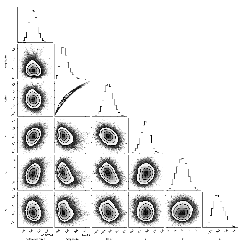
We find that the posterior distributions over the latent variables other than amplitude are typically well-described by a Gaussian distribution with a diagonal covariance matrix, and the predicted means and standard deviations that we obtain from variational inference are generally consistent with the true posterior distributions. This statement holds even for light curves that are only partially sampled, and we do not see any evidence of multi-modal posterior distributions. The amplitude and color latent variables are always highly correlated which justifies our decision to marginalize over the amplitude as described in Section 3.7. In general, we find that the posteriors estimated by variational inference are reasonably accurate, but it may be desirable to evaluate the full posteriors for applications such as supernova cosmology that require very high precision.

6.6 Applying the ParSNIP Model to Other Kinds of Light Curves

The model described in this paper was designed to be applied to short-lived transient light curves, and should not be applied to other kinds of light curves without modifications. In particular, the preprocessing procedure described in Section 2.1 roughly aligns and scales all of the light curves assuming that they have a well-defined maximum. This is not a valid assumption for sources such as variable stars or active galactic nuclei. We also subtract the background level of each light curve using observations away from maximum light, and we constrain the model to only output positive flux values. None of these assumptions are fundamental to the ParSNIP model, and they should all be adjusted as appropriate if applying the model to other kinds of light curves (e.g. not subtracting the background for variable stars).

6.7 Including Additional Observations in the Training

In this work we assumed that we only have photometry available for all of the light curves in our sample. Large spectroscopic followup campaigns are planned for most upcoming surveys. As an example, the 4MOST consortium projects that they will obtain 30,000 spectra of live transients (Swann et al., 2019). These spectra could be used to train the ParSNIP model. The ParSNIP model already predicts the spectra at every phase when the model is compared to photometry, and these model spectra could instead be compared to observed spectra directly.

When trained only on photometry, the ParSNIP model is required to learn spectra by deconvolving the photometry. Including spectra of even a subset of the transients would constrain the underlying spectral model. This would be especially helpful for rare transients, such as PS1-12baa discussed in Section 4.4, where there is limited photometry of similar transients to constrain the positions and widths of spectral features.

Additional followup photometry in different bands could similarly be included to constrain the model at wavelengths where spectral coverage is typically lacking, especially the UV and IR bands. Including a modest amount of IR photometry in the ParSNIP training dataset would allow ParSNIP to learn a coarse IR spectral model. Such models only currently exist for Type Ia supernovae, but are essential for simulating and planning upcoming experiments such as the Roman Space Telescope.

6.8 Combining Light Curves from Multiple Surveys

Transient light curves have been collected by many different surveys, and the ParSNIP model could be improved by training on a larger sample of light curves observed by different instruments. The neural network in the decoder of the ParSNIP model predicts spectra, and we explicitly compute photometry from those spectra using the known bandpasses for an instrument. As a result, the ParSNIP decoder can be used to predict the photometry for any instrument or bandpass without any modification to the architecture or neural network weights.

The ParSNIP encoder, on the other hand, treats all of the individual bandpasses separately. Nevertheless, it can operate on multiple instruments by adding additional channels to the input representing the individual bandpasses from each instrument. For instrument/bandpass combinations in which a transient was not observed, we input zero at all times. With this approach, the model can be trained simultaneously on light curves from different surveys to produce a single latent representation and decoder model that can be applied to all surveys. We tested this approach by training the ParSNIP model simultaneously on the PS1 and PLAsTiCC datasets. We found that the resulting model had a similar performance to the models trained on the individual datasets, and transients with the same label in both datasets are encoded at similar locations in the intrinsic representation.

7 Conclusions

The ParSNIP model developed in this work is a novel generative model that describes how the spectra of transients evolve over time. This model combines both a neural network to describe the intrinsic diversity of transients and an explicit physics model of how light from transients propagates through the universe and is observed. It can be trained using only a large dataset of light curves without requiring spectra or labels.

We demonstrated the effectiveness of our model both on both real (PS1) and simulated (PLAsTiCC) data. With a three-parameter intrinsic representation, we are able to reproduce out-of-sample light curves with model uncertainties of $\sim$0.06 mag for the PS1 dataset and $\sim$0.04 mag for the PLAsTiCC dataset. We also find that we are able to accurately predict the spectra of the transients despite only training on photometry. The ParSNIP model can estimate the distances to well-observed light curves of SNe Ia with an uncertainty of $0.150\pm 0.007$ mag compared to $0.155\pm 0.008$ mag for the SALT2 model on the same sample of SNe Ia.

Our model achieves state-of-the-art results for photometric classification. It produces an intrinsic representation that is independent of redshift, which means that it not highly sensitive to the biases in training sets that are a major challenge for other methods. For classification of SNe Ia, the ParSNIP model produces a sample that has 2 times less contamination compared to the SuperRAENN model on the PS1 dataset, and 2.3 times less contamination compared to the Avocado model on the PLAsTiCC dataset. The performance of the ParSNIP model is stable across all redshifts and does not require the use of techniques such as redshift augmentation. Our model can also be used to detect novel transients. In a simulated dataset, of 100 novel transients suggested by our algorithm, 90% of them are a new kind of transient that had never previously been observed.

All of the results in this paper can be reproduced with the publicly available parsnip software package . This package contains instructions for how to access all of the data that was used in our analyses. It also contains Jupyter notebooks that can be used to reproduce all of the figures in this paper.

References

- Alves et al. (2021) Alves, C. S., Peiris, H. V., Lochner, M., et al. 2021, arXiv e-prints, arXiv:2107.07531. https://arxiv.org/abs/2107.07531
- Astropy Collaboration et al. (2013) Astropy Collaboration, Robitaille, T. P., Tollerud, E. J., et al. 2013, A&A, 558, A33, doi: 10.1051/0004-6361/201322068
- Astropy Collaboration et al. (2018) Astropy Collaboration, Price-Whelan, A. M., Sipőcz, B. M., et al. 2018, AJ, 156, 123, doi: 10.3847/1538-3881/aabc4f
- Barbary (2016) Barbary, K. 2016, extinction v0.3.0, Zenodo, doi: 10.5281/zenodo.804967
- Barbary et al. (2016) Barbary, K., Biswas, R., Goldstein, G., et al. 2016, sncosmo, Zenodo, doi: 10.5281/zenodo.592747
- Bazin et al. (2009) Bazin, G., Palanque-Delabrouille, N., Rich, J., et al. 2009, A&A, 499, 653, doi: 10.1051/0004-6361/200911847
- Beers et al. (1990) Beers, T. C., Flynn, K., & Gebhardt, K. 1990, AJ, 100, 32, doi: 10.1086/115487
- Bepler et al. (2019) Bepler, T., Zhong, E., Kelley, K., Brignole, E., & Berger, B. 2019, in Advances in Neural Information Processing Systems, ed. H. Wallach, H. Larochelle, A. Beygelzimer, F. d'Alché-Buc, E. Fox, & R. Garnett, Vol. 32 (Curran Associates, Inc.). https://proceedings.neurips.cc/paper/2019/file/5a38a1eb24d99699159da10e71c45577-Paper.pdf
- Betoule et al. (2014) Betoule, M., Kessler, R., Guy, J., et al. 2014, A&A, 568, A22, doi: 10.1051/0004-6361/201423413
- Boone (2019) Boone, K. 2019, AJ, 158, 257, doi: 10.3847/1538-3881/ab5182
- Boone et al. (2021a) Boone, K., Aldering, G., Antilogus, P., et al. 2021a, ApJ, 912, 70, doi: 10.3847/1538-4357/abec3c
- Boone et al. (2021b) —. 2021b, ApJ, 912, 71, doi: 10.3847/1538-4357/abec3b
- Chambers et al. (2016) Chambers, K. C., Magnier, E. A., Metcalfe, N., et al. 2016, arXiv e-prints, arXiv:1612.05560. https://arxiv.org/abs/1612.05560
- Crenshaw & Connolly (2020) Crenshaw, J. F., & Connolly, A. J. 2020, AJ, 160, 191, doi: 10.3847/1538-3881/abb0e2
- Fitzpatrick & Massa (2007) Fitzpatrick, E. L., & Massa, D. 2007, ApJ, 663, 320, doi: 10.1086/518158
- Foreman-Mackey (2016) Foreman-Mackey, D. 2016, The Journal of Open Source Software, 1, 24, doi: 10.21105/joss.00024
- Foreman-Mackey et al. (2013) Foreman-Mackey, D., Hogg, D. W., Lang, D., & Goodman, J. 2013, PASP, 125, 306, doi: 10.1086/670067
- Graziani et al. (2020) Graziani, R., Rigault, M., Regnault, N., et al. 2020, arXiv e-prints, arXiv:2001.09095. https://arxiv.org/abs/2001.09095
- Guillochon et al. (2018) Guillochon, J., Nicholl, M., Villar, V. A., et al. 2018, ApJS, 236, 6, doi: 10.3847/1538-4365/aab761
- Guillochon et al. (2017) Guillochon, J., Parrent, J., Kelley, L. Z., & Margutti, R. 2017, ApJ, 835, 64, doi: 10.3847/1538-4357/835/1/64
- Guy et al. (2007) Guy, J., Astier, P., Baumont, S., et al. 2007, A&A, 466, 11, doi: 10.1051/0004-6361:20066930
- He et al. (2016) He, K., Zhang, X., Ren, S., & Sun, J. 2016, in 2016 IEEE Conference on Computer Vision and Pattern Recognition (CVPR), 770–778, doi: 10.1109/CVPR.2016.90
- Higgins et al. (2017) Higgins, I., Matthey, L., Pal, A., et al. 2017, in 5th International Conference on Learning Representations, ICLR 2017, Toulon, France, April 24-26, 2017, Conference Track Proceedings (OpenReview.net). https://openreview.net/forum?id=Sy2fzU9gl
- Hložek et al. (2020) Hložek, R., Ponder, K. A., Malz, A. I., et al. 2020, arXiv e-prints, arXiv:2012.12392. https://arxiv.org/abs/2012.12392
- Hlozek et al. (2012) Hlozek, R., Kunz, M., Bassett, B., et al. 2012, ApJ, 752, 79, doi: 10.1088/0004-637X/752/2/79
- Hosseinzadeh et al. (2020) Hosseinzadeh, G., Dauphin, F., Villar, V. A., et al. 2020, ApJ, 905, 93, doi: 10.3847/1538-4357/abc42b
- Hunter (2007) Hunter, J. D. 2007, Computing in Science & Engineering, 9, 90, doi: 10.1109/MCSE.2007.55
- Ishida et al. (2019) Ishida, E. E. O., Beck, R., González-Gaitán, S., et al. 2019, MNRAS, 483, 2, doi: 10.1093/mnras/sty3015
- Ishida et al. (2021) Ishida, E. E. O., Kornilov, M. V., Malanchev, K. L., et al. 2021, A&A, 650, A195, doi: 10.1051/0004-6361/202037709
- Ivezić et al. (2019) Ivezić, Ž., Kahn, S. M., Tyson, J. A., et al. 2019, ApJ, 873, 111, doi: 10.3847/1538-4357/ab042c
- Jones et al. (2018) Jones, D. O., Scolnic, D. M., Riess, A. G., et al. 2018, ApJ, 857, 51, doi: 10.3847/1538-4357/aab6b1
- Jones et al. (2001) Jones, E., Oliphant, T., Peterson, P., et al. 2001, SciPy: Open source scientific tools for Python. http://www.scipy.org/
- Ke et al. (2017) Ke, G., Meng, Q., Finley, T., et al. 2017, in Advances in Neural Information Processing Systems 30, ed. I. Guyon, U. V. Luxburg, S. Bengio, H. Wallach, R. Fergus, S. Vishwanathan, & R. Garnett (Curran Associates, Inc.), 3146–3154
- Kerzendorf et al. (2021) Kerzendorf, W. E., Vogl, C., Buchner, J., et al. 2021, ApJ, 910, L23, doi: 10.3847/2041-8213/abeb1b
- Kessler et al. (2019) Kessler, R., Narayan, G., Avelino, A., et al. 2019, PASP, 131, 094501, doi: 10.1088/1538-3873/ab26f1
- Kingma & Ba (2015) Kingma, D. P., & Ba, J. 2015, in 3rd International Conference on Learning Representations, ICLR 2015, San Diego, CA, USA, May 7-9, 2015, Conference Track Proceedings, ed. Y. Bengio & Y. LeCun. http://arxiv.org/abs/1412.6980
- Kingma & Welling (2014) Kingma, D. P., & Welling, M. 2014, in 2nd International Conference on Learning Representations, ICLR 2014, Banff, AB, Canada, April 14-16, 2014, Conference Track Proceedings, ed. Y. Bengio & Y. LeCun. http://arxiv.org/abs/1312.6114
- Kluyver et al. (2016) Kluyver, T., Ragan-Kelley, B., Pérez, F., et al. 2016, in Positioning and Power in Academic Publishing: Players, Agents and Agendas, ed. F. Loizides & B. Schmidt, IOS Press, 87 – 90
- Kulkarni et al. (2015) Kulkarni, T. D., Whitney, W. F., Kohli, P., & Tenenbaum, J. 2015, in Advances in Neural Information Processing Systems, ed. C. Cortes, N. Lawrence, D. Lee, M. Sugiyama, & R. Garnett, Vol. 28 (Curran Associates, Inc.). https://proceedings.neurips.cc/paper/2015/file/ced556cd9f9c0c8315cfbe0744a3baf0-Paper.pdf
- Kullback & Leibler (1951) Kullback, S., & Leibler, R. A. 1951, The Annals of Mathematical Statistics, 22, 79 , doi: 10.1214/aoms/1177729694
- Léget et al. (2020) Léget, P. F., Gangler, E., Mondon, F., et al. 2020, A&A, 636, A46, doi: 10.1051/0004-6361/201834954
- Lochner et al. (2016) Lochner, M., McEwen, J. D., Peiris, H. V., Lahav, O., & Winter, M. K. 2016, ApJS, 225, 31, doi: 10.3847/0067-0049/225/2/31
- LSST Science Collaboration et al. (2009) LSST Science Collaboration, Abell, P. A., Allison, J., et al. 2009, arXiv e-prints, arXiv:0912.0201. https://arxiv.org/abs/0912.0201
- Malz et al. (2019) Malz, A. I., Hložek, R., Allam, T., J., et al. 2019, AJ, 158, 171, doi: 10.3847/1538-3881/ab3a2f
- Mandel et al. (2020) Mandel, K. S., Thorp, S., Narayan, G., Friedman, A. S., & Avelino, A. 2020, arXiv e-prints, arXiv:2008.07538. https://arxiv.org/abs/2008.07538
- Martínez-Galarza et al. (2021) Martínez-Galarza, J. R., Bianco, F. B., Crake, D., et al. 2021, MNRAS, doi: 10.1093/mnras/stab2588
- Martínez-Palomera et al. (2020) Martínez-Palomera, J., Bloom, J. S., & Abrahams, E. S. 2020, arXiv e-prints, arXiv:2005.07773. https://arxiv.org/abs/2005.07773
- Möller & de Boissière (2020) Möller, A., & de Boissière, T. 2020, MNRAS, 491, 4277, doi: 10.1093/mnras/stz3312
- Muthukrishna et al. (2019) Muthukrishna, D., Narayan, G., Mandel, K. S., Biswas, R., & Hložek, R. 2019, PASP, 131, 118002, doi: 10.1088/1538-3873/ab1609
- Naul et al. (2018) Naul, B., Bloom, J. S., Pérez, F., & van der Walt, S. 2018, Nature Astronomy, 2, 151, doi: 10.1038/s41550-017-0321-z
- Pasquet et al. (2019) Pasquet, J., Pasquet, J., Chaumont, M., & Fouchez, D. 2019, A&A, 627, A21, doi: 10.1051/0004-6361/201834473
- Paszke et al. (2019) Paszke, A., Gross, S., Massa, F., et al. 2019, in Advances in Neural Information Processing Systems, ed. H. Wallach, H. Larochelle, A. Beygelzimer, F. d'Alché-Buc, E. Fox, & R. Garnett, Vol. 32 (Curran Associates, Inc.). https://proceedings.neurips.cc/paper/2019/file/bdbca288fee7f92f2bfa9f7012727740-Paper.pdf
- Pedregosa et al. (2011) Pedregosa, F., Varoquaux, G., Gramfort, A., et al. 2011, Journal of Machine Learning Research, 12, 2825
- Planck Collaboration et al. (2020) Planck Collaboration, Aghanim, N., Akrami, Y., et al. 2020, A&A, 641, A6, doi: 10.1051/0004-6361/201833910
- Pruzhinskaya et al. (2019) Pruzhinskaya, M. V., Malanchev, K. L., Kornilov, M. V., et al. 2019, MNRAS, 489, 3591, doi: 10.1093/mnras/stz2362
- Sanders et al. (2015) Sanders, N. E., Betancourt, M., & Soderberg, A. M. 2015, ApJ, 800, 36, doi: 10.1088/0004-637X/800/1/36
- Saunders et al. (2018) Saunders, C., Aldering, G., Antilogus, P., et al. 2018, ApJ, 869, 167, doi: 10.3847/1538-4357/aaec7e
- Schlafly & Finkbeiner (2011) Schlafly, E. F., & Finkbeiner, D. P. 2011, ApJ, 737, 103, doi: 10.1088/0004-637X/737/2/103
- Scolnic et al. (2018) Scolnic, D. M., Jones, D. O., Rest, A., et al. 2018, ApJ, 859, 101, doi: 10.3847/1538-4357/aab9bb
- Scovacricchi et al. (2016) Scovacricchi, D., Nichol, R. C., Bacon, D., Sullivan, M., & Prajs, S. 2016, MNRAS, 456, 1700, doi: 10.1093/mnras/stv2752
- Shivvers et al. (2019) Shivvers, I., Filippenko, A. V., Silverman, J. M., et al. 2019, MNRAS, 482, 1545, doi: 10.1093/mnras/sty2719
- Smartt et al. (2015) Smartt, S. J., Valenti, S., Fraser, M., et al. 2015, A&A, 579, A40, doi: 10.1051/0004-6361/201425237
- Spergel et al. (2015) Spergel, D., Gehrels, N., Baltay, C., et al. 2015, arXiv e-prints, arXiv:1503.03757. https://arxiv.org/abs/1503.03757
- Swann et al. (2019) Swann, E., Sullivan, M., Carrick, J., et al. 2019, The Messenger, 175, 58, doi: 10.18727/0722-6691/5129
- Tschannen et al. (2018) Tschannen, M., Bachem, O., & Lucic, M. 2018, arXiv e-prints, arXiv:1812.05069. https://arxiv.org/abs/1812.05069
- van der Walt et al. (2011) van der Walt, S., Colbert, S. C., & Varoquaux, G. 2011, Computing in Science and Engineering, 13, 22, doi: 10.1109/MCSE.2011.37
- Villar et al. (2021) Villar, V. A., Cranmer, M., Berger, E., et al. 2021, ApJS, 255, 24, doi: 10.3847/1538-4365/ac0893
- Villar et al. (2018) Villar, V. A., Nicholl, M., & Berger, E. 2018, ApJ, 869, 166, doi: 10.3847/1538-4357/aaee6a
- Villar et al. (2020) Villar, V. A., Hosseinzadeh, G., Berger, E., et al. 2020, ApJ, 905, 94, doi: 10.3847/1538-4357/abc6fd