Asynchronous Massive Access in Multi-cell Wireless Networks Using Reed-Muller Codes

Abstract

Providing connectivity to a massive number of devices is a key challenge in 5G wireless systems. In particular, it is crucial to develop efficient methods for active device identification and message decoding in a multi-cell network with fading, path loss, and delay uncertainties. This paper presents such a scheme using second-order Reed-Muller (RM) sequences and orthogonal frequency-division multiplexing (OFDM). For given positive integer $m$, a codebook is generated with up to $2^{m(m+3)/2}$ codewords of length $2^{m}$, where each codeword is a unique RM sequence determined by a matrix-vector pair with binary entries. This allows every device to send $m(m+3)/2$ bits of information where an arbitrary number of these bits can be used to represent the identity of a node, and the remaining bits represent a message. There can be up to $2^{m(m+3)/2}$ different identities. Using an iterative algorithm, an access point can estimate the matrix-vector pairs of each nearby device, as long as not too many devices transmit in the same frame. It is shown that both the computational complexity and the error performance of the proposed algorithm exceed another state-of-the-art algorithm. The device identification and message decoding scheme developed in this work can serve as the basis for grant-free massive access for billions of devices with hundreds of simultaneously active devices in each cell.

I Introduction

One of the promises of 5G wireless communication systems is to support large scale machine- type communication (MTC), that is, to provide connectivity to a massive number of devices as in the Internet of Things [1, 2, 3]. In massive MTC scenarios, the connection density will be up to $10^{6}$ devices per square kilometer [4]. A key characteristic of MTC is that the user traffic is typically sporadic so that in any given time interval, only a small fraction of devices are active. Also, short packets are the most common form of traffic generated by sensors and devices in MTC. This requires a fundamentally different design than that for supporting sustained high-rate mobile broadband communication.

A variety of effective multiple access techniques have been adopted in the previous and current cellular networks, such as frequency division multiple access (FDMA), time division multiple access (TDMA), code division multiple access (CDMA), and orthogonal frequency division multiple access (OFDMA) [5]. For these systems, resource blocks are orthogonally divided in time, frequency, or code domains. This makes signal detection at the access point (AP) fairly simple because the interference between adjacent blocks is minimized. However, due to the limitation of the number of orthogonal resource blocks, it can only support a limited number of devices. To provide connectivity to a massive number of devices, an information-theoretic paradigm called many-user access has been studied in [6, 7]. It was shown to be asymptotically optimal for active users to simultaneously transmit their identification signatures followed by their message bearing codewords. Further, various massive access schemes have been proposed; see examples [11, 12, 13, 29, 9, 10, 22, 26, 23, 24, 25, 18, 14, 15, 16, 19, 20, 21, 27, 28, 8, 30, 32, 33, 17, 31, 34] and references therein.

Indeed, active device identification and channel estimation are initial steps to enable message decoding in MTC. Due to the sporadic traffic in MTC, these problems are usually cast as neighbor discover or compressed sensing problems [35, 9, 10, 17, 8, 11, 12, 13, 14, 15, 16, 36, 37, 38, 41, 40, 39]. When the channel coefficients are known at the AP, several compressed sensing schemes were proposed for active device identification [41, 40, 39]. Further, approximate message passing (AMP)-based algorithms were applied for joint active device identification and channel estimation [14, 11, 12, 13, 15, 16]. In addition, greedy compressed sensing algorithm was designed for sparse signal recovery based on orthogonal matching pursuit [36, 37].

Another approach to the active device identification is slotted ALOHA. Recently, an enhanced random access scheme called coded slotted ALOHA was proposed in [42, 43], where each message is repeatedly sent over multiple slots, and information is passed between slots to recover messages lost due to collision. These works assume synchronized transmission and perfect interference cancelation. The asynchronous model has been studied in [44, 45]. It is pointed in [46] that slotted ALOHA only supports the detection of a single device within each slot. Instead, the authors in [46] proposed the $T$-fold ALOHA scheme such that the decoder can simultaneously decode up to $T$ messages in the same slot. By combining with serial interference cancellation, the performance of the $T$-fold ALOHA scheme is further improved in [47]. And [48, 33] proposed the $T$-fold ALOHA based random access scheme for handing Rayleigh fading channels and asynchronous transmission.

To identify the active device from an enormous number of potential users in the system, each device must be assigned a unique sequence. For a given positive integer $m$, a Reed-Muller (RM) code book is generated with up to $2^{m(m+3)/2}$ codewords of length $2^{m}$. The code book size is so large that every user is assigned a different signature in any practical system. Given this, RM sequence-based massive access schemes were proposed in [10, 9, 28, 27, 30, 29, 49]. In [27], a chirp detection algorithm for deterministic compressed sensing based on RM codes and associated functions was proposed. The authors in [28] have further enhanced the chirp detection algorithm with the slotting and patching framework. However, the algorithm in [28] works only for the additive white Gaussian noise (AWGN) channel (the channel estimation problem is thus not considered therein). For fading channels, an iterative RM device identification and channel estimation algorithm is adopted in [29] based on the derived nested structured of RM codes. In our previous work [49], we extend the real codebook used in [29] to the full codebook, which encodes more bits with little performance loss. In addition, when the number of active devices is large, the performance of the algorithm in [29] degrades dramatically. In contrast, by adopting slotting and message passing, the algorithm in [49] performs gracefully as the number of active devices increases. It can be proved that the worst-case complexities of RM codes-based detection algorithms are sub-linear in the number of codewords, which makes it an attractive algorithm for message decoding in MTC. The above RM detection algorithms are based on the assumption that the signals are synchronized. However, due to propagation delays in the practical environment, asynchrony cannot be ignored.

In this paper, we investigate the joint device identification/decoding and channel estimation in an asynchronous setting. By removing the unrealistic assumption of fully synchronous transmissions, the proposed scheme is an important step towards a practical design. In addition, 5G cellular systems are expected to deploy a large number of antennas to take advantage of massive multiple-input multiple-output (MIMO) technologies. Massive MIMO has been extensively studied to enable massive connectivity [11, 12, 13, 14, 15, 16, 50, 51, 52]. It can take advantage of the increased spatial degrees of freedom to support a large number of devices simultaneously. Since the user traffic is sporadic in MTC, [11, 12, 13, 14, 15, 16] proposes to formulate the device identification problem based on compressed sensing and thereby can be solved by the computationally efficient AMP algorithm. And a new pilot random access protocol called strongest-user collision resolution is proposed in [50, 51] to solve the intra-cell pilot collision in crowded massive MIMO systems. We note that algorithms using random codes and/or AMP type of decoding do not scale to millions of potential devices. Moreover, the preceding algorithms are based on the assumption that the signals are synchronized. As far as we know, there has been no research publications on asynchronous massive access with a large number of users and antennas. To fill this gap, we investigate asynchronous massive access in a multi-cell wireless network using Reed-Muller codes with many receive antennas which has the potential to support billions of potential devices in the network.

The main contributions are summarized as follows:

• Compared with the algorithms in [28, 27, 30, 29, 49] where transmitted signals are synchronized, we extend the algorithms to an asynchronous case where the arbitrary delays of each device are estimated based on the derived relationship between an RM sequence and its subsequences.

• To enhance the performance, we extend the RM detection algorithms to the case where the AP is deployed with a large number of antennas.

• We further describe an enhanced RM coding scheme with slotting and bit partition. The corresponding detection algorithm is referred to as Algorithm 1. We show that the computational complexity and performance of Algorithm 1 are notably improved, which makes it one important step closer to a practical algorithm.

• While many papers in the literature study massive access, this work is one of the few that can truly accommodate billions of devices and more.

The remainder of this paper is organized as follows. The system model is presented in Section II. Section III outlines the relationship between the RM sequence and its subsequences, which is the basis of the RM asynchronous decoding algorithm. Section IV displays the enhanced RM decoding algorithm utilizing slotting, message passing, and bit partition. Further, the computation complexity analysis is given in Section V. Section VI presents the numerical results, while Section VII concludes the paper.

Throughout the paper, boldface uppercase letters stand for matrices while boldface lowercase letters represent column vectors. The superscripts $(\cdot)^{\rm T}$, $(\cdot)^{*}$, and $(\cdot)^{\dagger}$ denote the transpose, complex conjugate, and conjugate transpose operator, respectively. The complex number field is denoted by $\mathbb{C}$. $\|\boldsymbol{x}\|_{p}$ denotes the $p$-norm of a vector $\boldsymbol{x}$, ${\|\boldsymbol{X}\|}_{F}$ denotes the Frobenius norm of a matrix $\boldsymbol{X}$, and $|A|$ denotes the cardinality of set $A$. $\boldsymbol{I}_{n}$ denotes an $n\times n$ identity matrix. $\lceil x\rceil$ represents the rounding function, which returns the smallest integer greater than $x$. $\odot$ means element-wise multiplication and ${\rm Arg}(\cdot)\in[-\pi,\pi)$ gives the phase angle of a complex number.

II System Model

II-A Transmission Scheme

Let $\Phi$ denote a large but finite set of devices on the plane with area $S$, where each device is equipped with one antenna. Further we denote ${\cal K}\subseteq\Phi$ as the active device set on the plane, each of which has $B$ bits to be sent. Due to the sporadic traffic in MTC, the number of active devices in a given time interval is far less than the total number of devices, i.e., $|{\cal K}|\ll|\Phi|$.

Prior to transmission, a message of $B$ bits is partitioned into $2^{d}$ sub-blocks, where the $j$-th sub-block consists $B_{j}$ information bits such that $\sum_{j=1}^{2^{d}}B_{j}=B$. To patch the information bits in different sub-blocks together, we adopt the tree encoder proposed in [55]. Specifically, the tree encoder appends $l_{j}$ parity bits to sub-block $j$, where the appended check bits satisfy random parity constraints associated with the message bits contained in the previous sub-blocks ($l_{1}=0$ in all cases). These parity check bits are needed to patch the information bits in different patches together, but they do not serve the purpose of transmitting the information. All the sub-blocks have the same size, i.e., $B_{j}+l_{j}=J$.

Assume there are $2^{p}$ time slots. Each active device randomly selects 2 slots to send its $J$ bits. We use $p$ bits to encode the location of the primary slot. And we use an arbitrary subset of size $p$ to encode a translate, which gives the secondary slot location when it is added to the primary slot location. To distinguish the primary and secondary slots, we fix a single check bit in the information bits to be 0 for the primary slot and 1 for the secondary slot. Thus deducing 1 bit from the total number of bits transmitted. Besides, in this paper, we deal with asynchronous transmission. To estimate the device delay, we assume two information bits to be zeros (To be specified in Section IV-B).

Fig. 1 depicts the transmission scheme where we set $d=1$ and $K=4$ for simplicity. In Fig. 1, each device has $B$ information bits to be sent. The information bits is first divided into $2^{d}$ sub-blocks. Each sub-block contains $B_{j}$ information bits, along with $l_{j}$ parity bits such that $J=B_{j}+l_{j}$. Then each device sent 2 copies of the $J$ bits in 2 randomly selected slots within the $2^{p}$ slots. Finally we perform the proposed decoding scheme and use tree decoder to patch together the information in different sub-blocks.

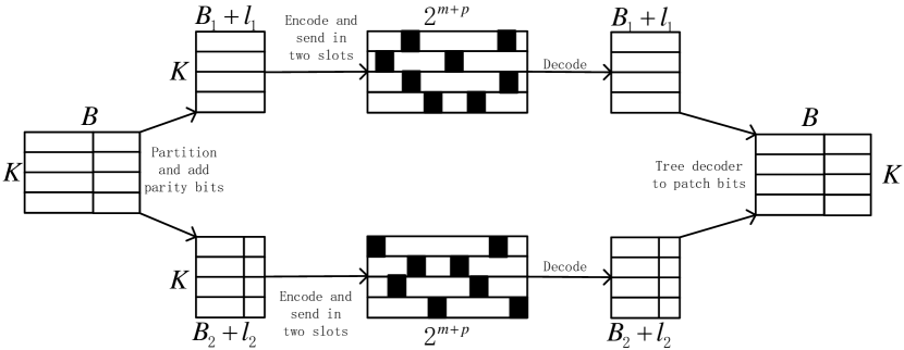
Figure 1: Illustration of the transmission scheme. We set $d=1$ and $K=4$ for simplicity.

II-B Encoding

Our approach is to encode these $J$ bits in each slot to a length $N=2^{m}$ second-order RM codes. A length $2^{m}$ second-order RM sequence is determined by a symmetric binary matrix $\boldsymbol{P}^{m}\in{\mathbb{Z}}_{2}^{m\times m}$ and a binary vector $\boldsymbol{b}^{m}\in{\mathbb{Z}}_{2}^{m}$. Since $\boldsymbol{P}^{m}$ is determined by $\frac{1}{2}m(m+1)$ bits and $\boldsymbol{b}^{m}$ is determined by $m$ bits, each sequence encodes $\frac{1}{2}m(m+3)$ bits. Given the matrix-vector pair $(\boldsymbol{P}^{m},\boldsymbol{b}^{m})$, the $n$-th entry of the RM sequence $\boldsymbol{X}^{m}$ can be written as [28]

$$\begin{split}X^{m}_{n}={\iota}^{2(\boldsymbol{b}^{m})^{\rm T}\boldsymbol{a}_{n-1}^{m}+(\boldsymbol{a}_{n-1}^{m})^{\rm T}\boldsymbol{P}^{m}\boldsymbol{a}_{n-1}^{m}},\quad n=1,\cdots,N,\end{split}$$ (1)

where $\iota^{2}=-1$, $\boldsymbol{a}_{n-1}^{m}$ is the $m$-bit binary expression of $(n-1)$. Eq. (1) indicates that $X^{m}_{n}\in\{1,-1,\iota,-\iota\}$.

In this case, we have

$$J=\frac{1}{2}m(m+1)+p-3.$$ (2)

Further, the number of information bits is written as

$$B=2^{d}\left(\frac{1}{2}m(m+3)+p-3\right)-\sum\limits_{j=1}^{2^{d}}l_{j}$$ (3)

II-C Channel Model

In this paper, we consider OFDM modulation where each symbol consists of $N$ subcarriers. Denote the frequency samples of device $k$ as $X_{k,n}^{m}$ where $n=1,2,\cdots,N$ is the subcarrier index. As explained before, $X_{k,n}^{m}$ is a RM sequence generated by (1). The time-domain OFDM symbol of device $k$ can be written as

$$x_{k}(t)=\sqrt{\gamma}\sum_{n=1}^{N}X_{k,n}^{m}{\rm e}^{2\pi\iota\Delta fnt},\quad t\in\left[0,\frac{1}{\Delta f}+\tau_{\rm max}\right],$$ (4)

where $\Delta f$ is the carrier spacing and the symbol duration is $1/\Delta f$ and $\tau_{\rm max}$ is the maximum device delay. $X_{k,n}^{m}$ is device $k$’s sample to be transmitted in subcarrier $n$. $\gamma$ denotes the transmit power.

We denote ${\cal K}_{i}$ as the active device set that transmitted in time slot $i$. Let $K=|{\cal K}|,K_{i}=|{\cal K}_{i}|$, we have $K_{i}\approx 2K/2^{p}$ since each device randomly choose 2 slots in the $2^{p}$ time slots. Without loss of generality, we assume the index of the active devices in slot $i$ is ${\cal K}_{i}=\{1,2,\cdots,K_{i}\}$. We focus on one AP equipped with $r$ antennas, and assume that the AP is located at the origin of the plane. The receive signal of the $l$-th antenna of the AP at time slot $i$ is written as

$$y_{l,i}(t) =\sum_{k=1}^{K_{i}}h_{k,l}x_{k}(t-\tau_{k})+z_{l,i}(t),$$ (5)

where $\boldsymbol{h}_{k}=[h_{k,1},\cdots,h_{k,r}]^{\rm T}$ is the channel vector between device $k$ and the AP and $z_{l}(t)$ is additive white Gaussian noise; $\tau_{k}$ is the transmission delay and $x_{k}(t)$ is the transmit signal of device $k$.

Then the AP samples at time $\frac{1}{\Delta f}\frac{u}{N},u=1,\cdots,N+\left\lceil\tau_{\rm max}N\Delta f\right\rceil$. The total number of samples in each slot is thus $N+M$ where $M=\left\lceil\tau_{\rm max}N\Delta f\right\rceil$ is the length of cyclic prefix. Furthermore, the total codelength can be written as

$$C=2^{d+p}(N+M).$$ (6)

Then the AP discard the first $M$ cyclic prefix in the OFDM symbol to form the discrete-time receive signal

$$y_{l,i}(u)=\sqrt{\gamma}\sum_{k=1}^{K_{i}}h_{k,l}\sum_{n=1}^{N}X_{k,n}^{m}{\rm e}^{-\iota\Delta_{k}n}{\rm e}^{\iota\frac{2\pi}{N}nu}+z_{l,i}(u),\quad u=1,\cdots,N,$$ (7)

where $\Delta_{k}=2\pi\Delta f\tau_{k}$ is the normalized delay; $z_{l,i}(u)\sim{\cal CN}(0,1)$. We assume the normalized delay is uniformly distributed in $\Delta_{k}\in[-\pi,\pi]$.

Performing $N$ point DFT on $[y_{l,i}(1),\cdots,y_{l,i}(N)]^{\rm T}$ yields

$$Y_{l,i}^{m}(n) =\sqrt{\gamma}\sum_{k=1}^{K_{i}}h_{k,l}\frac{1}{N}\sum_{u=1}^{N}{\rm e}^{-\iota\frac{2\pi}{N}nu}\sum_{v=1}^{N}X_{k,v}{\rm e}^{-\iota\Delta_{k}v}{\rm e}^{\iota\frac{2\pi}{N}uv}+Z_{l,n}^{m}(u)$$ (8)

$$=\sqrt{\gamma}\sum_{k=1}^{K_{i}}h_{k,l}X_{k,n}{\rm e}^{-\iota\Delta_{k}n}+Z_{l,i}^{m}(n),$$ (9)

where

$$Z_{l,i}^{m}(n) =\frac{1}{N}\sum_{u=1}^{N}{\rm e}^{-\iota\frac{2\pi}{N}nu}z_{l,i}(u)\sim{\cal CN}(0,1).$$ (10)

and $n=1,\cdots,N$ and $l=1,\cdots,r$.

Let $\boldsymbol{Y}_{i}^{m}(n)=[Y_{1,i}^{m}(n),\cdots,Y_{r,i}^{m}(n)]^{\rm T}$. For simplicity, denote $\boldsymbol{Y}_{i}^{m}=\left[\boldsymbol{Y}_{i}^{m}(1),\cdots,\boldsymbol{Y}_{i}^{m}(N)\right]$ as the DFT results in slot $i$.

II-D Propagation Model and Cell Coverage

Consider a multiaccess channel with active devices distributed across the plane according to a homogeneous Poisson point process with intensity $\lambda$. The number of active devices on the plane with its area equal to $S$ is a Poisson random variable with mean $\lambda S\approx|\cal K|$.

We further divide the active device set ${\cal K}$ into in-cell device set (neighbor) and out-of-the-cell device set (non-neighbor) of the AP according to the nominal SNR between the AP and the devices. If the nominal SNR between a device and the AP is larger than a threshold, then this device is considered an in-cell device of the AP. The purpose of the AP is to identify all in-cell devices and/or decode their messages, where transmissions from out-of-the-cell devices are regarded as interference.

The small-scale fading between the device and the AP is modeled by an independent Rayleigh random variable with unit mean. The large-scale fading is modeled by the free-space path loss which attenuates over distance with some path loss exponent $\alpha>2$.

Let $D_{k}$ and $\boldsymbol{G}_{k}=[G_{k,1},\cdots,G_{k,r}]^{\rm T}$ denotes the distance and the small scale Rayleigh fading gain between device $k,k=1,2,\cdots,K$, and the AP, respectively. Then the channel gain between device $k$ and the $l$-th antenna of the AP is expressed as

$$\begin{split}|h_{k,l}|^{2}=D_{k}^{-\alpha}G_{k,l},\end{split}$$ (11)

where the phase of $h_{k,l}$ is uniformly distributed on $[0,2\pi)$.

The coverage of the AP can be defined in many different ways. According to [53], device $k$ and the AP are neighbors of each other if the channel gain exceeds a certain threshold $\theta$. Assume device $k$ and the AP are neighbors, i.e., $D_{k}^{-\alpha}\|\boldsymbol{G}_{k}\|_{1}>r\theta$, we have $D_{k}<\left({\frac{\|\boldsymbol{G}_{k}\|_{1}}{r\theta}}\right)^{1/{\alpha}}$. Under the assumption that all devices form a p.p.p., for given $\boldsymbol{G}_{k}$, device $k$ is uniformly distributed in a disk centered at the AP with radius $\left({\frac{\|\boldsymbol{G}_{k}\|_{1}}{r\theta}}\right)^{1/{\alpha}}$. The average number of neighbors of the AP is calculated as

$$K^{*} =\mathbb{E}_{\boldsymbol{\Phi}}\left\{\sum\limits_{k\in\boldsymbol{\Phi}}1(D_{k}^{-\alpha}\|\boldsymbol{G}_{k}\|_{1}\geq r\theta)\right\}$$ (12)

$$=2\pi\lambda\int_{0}^{\infty}\int_{0}^{\infty}1(gs^{-\alpha}\geq r\theta)s\frac{1}{\Gamma(r)}g^{r-1}{\rm e}^{-g}{\rm d}s{\rm d}g$$ (13)

$$=2\pi\lambda\int_{0}^{\infty}\int_{0}^{\left(\frac{g}{r\theta}\right)^{\frac{1}{\alpha}}}s\frac{1}{\Gamma(r)}g^{r-1}{\rm e}^{-g}{\rm d}s{\rm d}g$$ (14)

$$=\pi\lambda\int_{0}^{\infty}\left(\frac{g}{r\theta}\right)^{\frac{2}{\alpha}}\frac{1}{\Gamma(r)}g^{r-1}{\rm e}^{-g}{\rm d}g$$ (15)

$$=\pi\lambda(r\theta)^{-\frac{2}{\alpha}}\frac{\Gamma\left(\frac{2}{\alpha}+r\right)}{\Gamma(r)}$$ (16)

where $\Gamma(\cdot)$ is the Gamma function and $1(\cdot)$ is the indicator function. Eq. (16) indicates that $K^{*}$ is an increasing function of $r$.

In addition, the sum power of all out-of-the-cell devices can be derived as

$$\sigma^{2} =\mathbb{E}_{\boldsymbol{\Phi}}\left\{\sum\limits_{k\in\boldsymbol{\Phi}}1(D_{k}^{-\alpha}\|\boldsymbol{G}_{k}\|_{1}<r\theta)\gamma D_{k}^{-\alpha}\|\boldsymbol{G}_{k}\|_{1}\right\}$$ (17)

$$=2\pi\lambda\gamma\int_{0}^{\infty}\int_{0}^{\infty}gs^{-\alpha}1(gr^{-\alpha}<r\theta)s\frac{1}{\Gamma(r)}g^{r-1}{\rm e}^{-g}{\rm d}s{\rm d}g$$ (18)

$$=2\pi\lambda\gamma\int_{0}^{\infty}\int_{\left(\frac{g}{r\theta}\right)^{\frac{1}{\alpha}}}^{\infty}s^{1-\alpha}\frac{1}{\Gamma(r)}g^{r}{\rm e}^{-g}{\rm d}s{\rm d}g$$ (19)

$$=\frac{2\pi\lambda\gamma}{\alpha-2}\int_{0}^{\infty}\left(\frac{g}{r\theta}\right)^{\frac{2-\alpha}{\alpha}}\frac{1}{\Gamma(r)}g^{r}{\rm e}^{-g}{\rm d}g$$ (20)

$$=(r\theta)^{1-2/\alpha}\frac{2\pi\lambda\gamma}{(\alpha-2)}\frac{\Gamma\left(\frac{2}{\alpha}+r\right)}{\Gamma(r)}$$ (21)

III A Property of RM Sequences

Before given the decoding algorithm, we first derive a property of RM sequence, which is the basis of our decoding algorithm.

Let $m$ be a given positive number. Let $\boldsymbol{b}^{s}=[b^{m}_{1},b_{2}^{m},\cdots,b_{s}^{m}]^{\rm T}$ be a binary $s$-tuple. For $s=2,\cdots,m$, we have

$$\begin{split}\boldsymbol{b}^{s}=\left[\begin{array}[]{c}\boldsymbol{b}^{s-1}\\ b_{s}^{m}\end{array}\right].\end{split}$$ (22)

Furthermore, let $P^{1}=[\beta^{m}_{1}]$. For $s=2,\cdots,m$, let the $s\times s$ binary matrix $\boldsymbol{P}^{s}$ be defined recursively as

$$\begin{split}\boldsymbol{P}^{s}=\left[\begin{array}[]{cccc}\boldsymbol{P}^{s-1}&\boldsymbol{\eta}^{s}\\ (\boldsymbol{\eta}^{s})^{\rm T}&\beta^{m}_{s}\end{array}\right]\end{split},$$ (23)

where $[\beta^{m}_{1},\beta_{2}^{m},\cdots,\beta_{s}^{m}]^{\rm T}$ is the main diagonal elements of $\boldsymbol{P}^{s}$, and $\boldsymbol{\eta}^{s}$ is a length $s-1$ column vector.

We have the following result.

Proposition 1.

Given a length-$2^{m}$ RM sequence, its order $s$ and $s-1$ sub-sequences satisfy

$$\begin{split}\left\{\begin{array}[]{l}X^{s}_{2n}=V_{n}^{s-1}X_{n}^{s-1}\\ X^{s}_{2n-1}=X_{n}^{s-1}\end{array}\right.,\quad n=1,\cdots,2^{s-1},s=2,\cdots,m\end{split}$$ (24)

where

$$V_{n}^{s-1} =(-1)^{b_{s}^{m}+\frac{1}{2}\beta_{s}^{m}+(\boldsymbol{\eta}^{s})^{\rm T}\boldsymbol{a}_{n-1}^{s-1}}.$$ (25)

The vector $[V_{1}^{s-1},\cdots,V_{2^{s-1}}^{s-1}]^{\rm T}$ is a length-$2^{s-1}$ Walsh sequence with frequency $\boldsymbol{\eta}^{s}$.

Proof:

Recall $a_{n}^{s}$ is the $s$-bit expression of $n$. For $n=1,\cdots,2^{s-1}$, the vector $\boldsymbol{a}_{2n-1}^{s}$ can be decomposed as

$$\begin{split}\boldsymbol{a}_{2n-1}^{s}=\left[\begin{array}[]{c}\boldsymbol{a}_{n-1}^{s-1}\\ 1\end{array}\right].\end{split}$$ (26)

Consequently

$$2(\boldsymbol{b}^{s})^{\rm T}\boldsymbol{a}_{2n-1}^{s}+(\boldsymbol{a}_{2n-1}^{s})^{\rm T}\boldsymbol{P}^{s}\boldsymbol{a}_{2n-1}^{s}$$

$$=\left[\begin{array}[]{cc}\left(\boldsymbol{a}_{n-1}^{s-1}\right)^{\rm T}&1\end{array}\right]\left[\begin{array}[]{cccc}\boldsymbol{P}^{s-1}&\boldsymbol{\eta}^{s}\\ (\boldsymbol{\eta}^{s})^{\rm T}&\beta^{m}_{s}\end{array}\right]\left[\begin{array}[]{c}\boldsymbol{a}_{n-1}^{s-1}\\ 1\end{array}\right]+2(\boldsymbol{b}^{s})^{\rm T}\left[\begin{array}[]{c}\boldsymbol{a}_{n-1}^{s-1}\\ 1\end{array}\right]$$ (34)

$$=2(\boldsymbol{b}^{s-1})^{\rm T}\boldsymbol{a}_{n-1}^{s-1}\!+2b_{s}^{m}\!+\beta_{s}^{m}+\!2(\boldsymbol{\eta}^{s})^{\rm T}\boldsymbol{a}_{n-1}^{s-1}\!+\left(\boldsymbol{a}_{n-1}^{s-1}\right)^{\rm T}\!\boldsymbol{P}^{s-1}\boldsymbol{a}_{n-1}^{s-1}.$$ (35)

Substituting (35) into (1) yields

$$X^{s}_{2n} =X_{n}^{s-1}\iota^{2b_{s}^{m}+\beta_{s}^{m}+2(\boldsymbol{\eta}^{s})^{\rm T}\boldsymbol{a}_{n-1}^{s-1}}$$ (36)

$$=V_{n}^{s-1}X_{n}^{s-1}.$$ (37)

Likewise, the binary vector $\boldsymbol{a}_{2j-2}^{s}$ can be decomposed as

$$\begin{split}\boldsymbol{a}_{2n-2}^{s}=\left[\begin{array}[]{c}\boldsymbol{a}_{n-1}^{s-1}\\ 0\end{array}\right]\end{split}.$$ (38)

Then the exponent of $X^{s}_{2n-1}$ is expressed as

$$2(\boldsymbol{b}^{s})^{\rm T}\boldsymbol{a}_{2n-2}^{s}+(\boldsymbol{a}_{2n-2}^{s})^{\rm T}\boldsymbol{P}^{s}\boldsymbol{a}_{2n-2}^{s}$$

$$=\left[\begin{array}[]{cc}\left(\boldsymbol{a}_{n-1}^{s-1}\right)^{\rm T}&0\end{array}\right]\left[\begin{array}[]{cccc}\boldsymbol{P}^{s-1}&\boldsymbol{\eta}^{s}\\ (\boldsymbol{\eta}^{s})^{\rm T}&\beta_{s}^{m}\end{array}\right]\left[\begin{array}[]{c}\boldsymbol{a}_{n-1}^{s-1}\\ 0\end{array}\right]+2(\boldsymbol{b}^{s})^{\rm T}\left[\begin{array}[]{c}\boldsymbol{a}_{n-1}^{s-1}\\ 0\end{array}\right]$$ (46)

$$=2(\boldsymbol{b}^{s-1})^{\rm T}\boldsymbol{a}_{n-1}^{s-1}+\left(\boldsymbol{a}_{n-1}^{s-1}\right)^{\rm T}\boldsymbol{P}^{s-1}\boldsymbol{a}_{n-1}^{s-1}.$$ (47)

Substituting (47) into (1) yields

$$\begin{split}X^{s}_{2n-1}=X_{n}^{s-1}.\end{split}$$ (48)

∎

Remark 1: The structure of the derived RM sequence is similar to that of given in [29]. The differences are two folds: 1) given the code length $2^{m}$, compared with the structure given in [29], the structure given in this paper allows us to send $2m$ more bits of information; 2) the way we splitting the sequences is different.

IV Device Identification/Decoding and Channel Estimation

In this section, we propose a novel RM asynchronous detection algorithm for active device detection and channel estimation that leverages Proposition 1.

IV-A RM Asynchronous Detection Algorithm

According to Fig. 1, the AP decodes the messages in different sub-blocks in a sequential manner. In each sub-block, the AP decodes the messages slot-by-slot. Since each device transmits in 2 time slots, the message decoded in the previous time slot will be propagated to another time slot to eliminate its interference.

The detailed algorithm is summarized as in Algorithm 1.

Algorithm 1: RM asynchronous detection algorithm.

Input: the received signal $[\boldsymbol{Y}^{q}_{1},\cdots,\boldsymbol{Y}^{q}_{2^{p}}]$, the average number of devices $K_{\rm max}$ in each

slot.

for $patch=1:2^{d}$ do

Set $\boldsymbol{P}=[\ ]$, $\boldsymbol{b}=[\ ]$, $slot=[\ ],\boldsymbol{h}=[\ ]$, $\boldsymbol{\Delta}=[\ ]$, $t=0$.

for $i=1:2^{p}$ do

$k\leftarrow 0$.

for $j=1:s$ do

if $slot[j]=i$ do

Remove the interference of device $j$ in slot $i$ and update $\boldsymbol{Y}^{q}_{i}$ according to (51).

$t\leftarrow t+1$.

end if

end for

$(\hat{\boldsymbol{P}}^{m},\hat{\boldsymbol{b}}^{m},\hat{\boldsymbol{h}},\hat{\Delta})\leftarrow{\bf findPb}\ (\boldsymbol{Y}_{i}^{q})$.

Denote $k_{1}$ as the number of detected messages in slot $i$.

for $j=1:k_{1}$

if $(\hat{\boldsymbol{P}}_{j}^{m},\hat{\boldsymbol{b}}_{j}^{q})$ are not recorded in $(\boldsymbol{P},\boldsymbol{b})$ do

$t\leftarrow t+1$.

$\boldsymbol{P}[:,:,t]\leftarrow\hat{\boldsymbol{P}}_{j}^{m}$.

$\boldsymbol{b}[:,t]\leftarrow\hat{\boldsymbol{b}}_{j}^{m}$.

$\boldsymbol{h}[:,t]\leftarrow\hat{\boldsymbol{h}}_{j}$.

$\boldsymbol{\Delta}[t]\leftarrow\hat{\Delta}_{j}$.

Calculate the translate according to $\left(\hat{\boldsymbol{P}}_{j}^{q},\hat{\boldsymbol{b}}_{j}^{q}\right)$ and update $slot[s]$.

end if

end for

end for

Record $\boldsymbol{P},\boldsymbol{b},\boldsymbol{h}$, and $\boldsymbol{\Delta}$ in each sub-block.

end for

Output: Using tree decoder to patch the information bits together and output.

The findPb algorithm in Algorithm 1 returns all the messages transmitted in slot $i$, including the information bits $(\boldsymbol{P},\boldsymbol{b})$, the channel vector $\boldsymbol{h}$, and the device delay $\Delta$. The findPb algorithm decodes the messages transmitted in slot $i$ in a sequential manner. Assume the channel gain of device $k\in\{1,\cdots,K_{i}\}$ is the biggest. We will show that device $k$ can be first estimated from the received signal (9). After device $k$ is detected, the AP performs successive interference cancellation (SIC) to remove the interference of device $k$ to detect the remaining devices. This requires the AP to estimate not only the matrix-vector pair $(\boldsymbol{P}_{k}^{m},\boldsymbol{b}_{k}^{m})$, but also the device delay $\Delta_{k}$. In this paper, to estimate the device delay, we let

$$b_{l,m}^{m}=\beta_{l,m}^{m}=0,\quad l=1,\cdots,K_{i}.$$ (49)

For simplicity, let $\boldsymbol{\Delta}_{k}^{m}=[\Delta_{k,1}^{m},\cdots,\Delta_{k,m}^{m}]$, where

$$\Delta_{k,l}^{m}={\rm Arg}\left({\rm e}^{2^{l-1}j\Delta_{k}}\right),\quad l=1,\cdots,m.$$ (50)

In the next section, we show how to estimate the messages of device $k$.

IV-B The findPb Algorithm

According to (22) and (23), the matrix-vector pair $(\boldsymbol{P}^{m},\boldsymbol{b}^{m})$ is determined by $(\boldsymbol{\eta}^{s},b_{s}^{m},\beta_{s}^{m}),s=m,\cdots,2$ and $(b_{1}^{m},\beta_{1}^{m})$. Specifically, the matrix-vector pair of the $k$th device $(\boldsymbol{P}_{k}^{m},\boldsymbol{b}_{k}^{m})$ will be estimated recursively. We will show that the algorithm first estimates $\boldsymbol{\eta}_{k}^{m}$, then $(\boldsymbol{\eta}_{k}^{m-1},b_{k,m-1}^{m},\beta_{k,m-1}^{m})$, and finally the channel coefficient $\boldsymbol{h}_{k}$, $(b_{k,1}^{m},\beta_{k,1}^{m})$, and ${\Delta}_{k}$.

Then the receiver signal in slot $i$ is updated as

$$\boldsymbol{Y}_{i}^{m}(n)\leftarrow\boldsymbol{Y}_{i}^{m}(n)-\sqrt{\gamma}\boldsymbol{h}_{k}X_{k,n}^{m}{\rm e}^{-j\Delta_{k}n},$$ (51)

for detecting the remaining devices.

IV-B1 Estimation of $(\boldsymbol{\eta}_{k}^{m},\Delta_{k,1}^{m})$

From (9) and (24), when $n=1,\cdots,2^{m-1}$, we have

$$\boldsymbol{Y}_{i}^{m}(2n) =\sqrt{\gamma}\sum_{k=1}^{K_{i}}\boldsymbol{h}_{k}X_{k,2n}^{m}{\rm e}^{-2j\Delta_{k}n}+\boldsymbol{Z}_{i}^{m}(2n)$$ (52)

$$=\sqrt{\gamma}\sum_{k=1}^{K_{i}}\boldsymbol{h}_{k}V_{k,n}^{m-1}X_{k,n}^{m-1}{\rm e}^{-2j\Delta_{k}n}+\boldsymbol{Z}_{i}^{m}(2n),$$ (53)

and

$$\boldsymbol{Y}_{i}^{m}(2n-1) =\sqrt{\gamma}\sum_{k=1}^{K_{i}}\boldsymbol{h}_{k}X_{k,2n-1}^{m}{\rm e}^{-j\Delta_{k}(2n-1)}+\boldsymbol{Z}_{i}^{m}(2n-1)$$ (54)

$$=\sqrt{\gamma}\sum_{k=1}^{K_{i}}\boldsymbol{h}_{k}X_{k,n}^{m-1}{\rm e}^{-j\Delta_{k}(2n-1)}+\boldsymbol{Z}_{i}^{m}(2n-1).$$ (55)

Define $\tilde{Y}_{n}^{m-1}=[\boldsymbol{Y}_{i}^{m}(2n)]^{\rm T}[\boldsymbol{Y}_{i}^{m}(2n-1)]^{*}$ for $n=1,\cdots,2^{m-1}$, (53) and (55) lead to

$$\tilde{Y}_{n}^{m-1} =\gamma\sum_{k=1}^{K_{i}}\left\|\boldsymbol{h}_{k}X_{k,n}^{m-1}\right\|^{2}V_{k,n}^{m-1}{\rm e}^{-j\Delta_{k}}+\tilde{Z}_{n}^{m-1}$$ (56)

$$=\gamma\sum_{k=1}^{K_{i}}\|\boldsymbol{h}_{k}\|^{2}V_{k,n}^{m-1}{\rm e}^{-j\Delta_{k}}+\tilde{Z}_{n}^{m-1},$$ (57)

where

$$\begin{split}\tilde{Z}_{n}^{m-1}&=\gamma\sum_{l=1}^{K_{i}}\sum_{k\neq l}\boldsymbol{h}_{k}^{\rm T}V_{k,n}^{m-1}X_{k,n}^{m-1}(\boldsymbol{h}_{l}X_{l,n}^{m-1})^{*}{\rm e}^{-2j\Delta_{k}n}{\rm e}^{j\Delta_{l}(2n-1)}\\ &+\sqrt{\gamma}\sum_{k=1}^{K_{i}}\boldsymbol{h}_{k}^{\rm T}V_{k,n}^{m-1}X_{k,n}^{m-1}{\rm e}^{-2j\Delta_{k}n}(\boldsymbol{Z}_{i}^{m}(2n-1))^{*}\\ &+\sqrt{\gamma}(\boldsymbol{Z}_{i}^{m}(2n))^{\rm T}\sum_{l=1}^{K_{i}}(\boldsymbol{h}_{l}X_{l,n}^{m-1}{\rm e}^{-j\Delta_{k}(2n-1)})^{*}+(\boldsymbol{Z}_{i}^{m}(2n))^{\rm T}(\boldsymbol{Z}_{i}^{m}(2n-1))^{*}.\end{split}$$ (58)

The first term in the right-hand side of (57) is a linear combination of Walsh functions $V_{k,n}^{m-1},k=1,2,\cdots,K$, with frequency $\boldsymbol{\eta}^{m}_{k}$, which can be recovered by applying Walsh-Hadamard Transformation (WHT). The second term, $\tilde{Z}_{n}^{m-1}$, is a linear combination of chirps, which can be considered to be distributed across all Walsh functions to equal degree, and therefore these cross-terms appear as a uniform noise floor.

Let the Hadamard matrix be $\boldsymbol{W}^{m}=\left[\boldsymbol{w}_{1}^{m},\boldsymbol{w}_{2}^{m},\cdots,\boldsymbol{w}_{2^{m}}^{m}\right]^{\rm T}$ and its $(l,n)$-th elements are $\boldsymbol{W}_{l,n}^{m}=(-1)^{(\boldsymbol{a}_{l-1}^{m})^{\rm T}{\boldsymbol{a}_{n-1}^{m}}}$. Denote the WHT transformation as $\boldsymbol{t}^{m-1}=\boldsymbol{W}^{m-1}\tilde{\boldsymbol{Y}}^{m-1}$, where $\tilde{\boldsymbol{Y}}^{m-1}=[\tilde{Y}_{1}^{m-1},\cdots,\tilde{Y}_{2^{m-1}}^{m-1}]$. The $l$-th entry of $\boldsymbol{t}^{m-1}$ can be written as

$$t_{l}^{m-1} =(\boldsymbol{w}_{l}^{m-1})^{\rm T}\tilde{\boldsymbol{Y}}^{m-1}$$ (59)

$$=\sum_{n=1}^{2^{m-1}}(-1)^{(\boldsymbol{a}_{l-1}^{m-1})^{\rm T}{\boldsymbol{a}_{n-1}^{m-1}}}\left(\gamma\sum_{k=1}^{K_{i}}\|\boldsymbol{h}_{k}\|^{2}V_{k,n}^{m-1}{\rm e}^{-j\Delta_{k}}\!+\!\tilde{Z}_{n}^{m-1}\right)$$ (60)

$$=\gamma\sum_{n=1}^{2^{m-1}}(-1)^{\left(\boldsymbol{a}_{l-1}^{m-1}\right)^{\rm T}{\boldsymbol{a}_{j-1}^{m-1}}}\sum_{k=1}^{K_{i}}{\rm e}^{-j\Delta_{k}}\|\boldsymbol{h}_{k}\|^{2}(-1)^{b_{k,m}^{m}+\frac{1}{2}\beta_{k,m}^{m}+(\boldsymbol{\eta}_{k}^{m})^{\rm T}\boldsymbol{a}_{n-1}^{m-1}}$$

$$+\sum_{n=1}^{2^{m-1}}(-1)^{(\boldsymbol{a}_{l-1}^{m-1})^{\rm T}{\boldsymbol{a}_{n-1}^{m-1}}}\tilde{Z}_{n}^{m-1}$$ (61)

Equation (61) can be further written as

$$t_{l}^{m-1} =\gamma\sum_{k=1}^{K}(-1)^{b_{k,m}^{m}+\frac{1}{2}\beta_{k,m}^{m}}{\rm e}^{-j\Delta_{k}}\|\boldsymbol{h}_{k}\|^{2}\sum_{n=1}^{2^{m-1}}(-1)^{\left(\boldsymbol{\eta}_{k}^{m}+\boldsymbol{a}_{l-1}^{m-1}\right)^{\rm T}{\boldsymbol{a}_{n-1}^{m-1}}}$$

$$+\sum_{n=1}^{2^{m-1}}(-1)^{(\boldsymbol{a}_{l-1}^{m-1})^{\rm T}{\boldsymbol{a}_{n-1}^{m-1}}}\tilde{Z}_{n}^{m-1}.$$ (62)

Equation (62) indicates that, if we have $\boldsymbol{\eta}_{k}^{m}=\boldsymbol{a}_{l-1}^{m-1}$, peaks will appear at frequency $\boldsymbol{\eta}^{m}_{k},k\in\{1,2,\cdots,{K_{i}}\}$, where the maximum value is ${\rm e}^{-j\Delta_{k}}2^{m-1}\gamma|\boldsymbol{h}_{k}|^{2}$. On this basis, $\boldsymbol{\hat{\eta}}_{k}^{m}$ can be recovered by searching the largest absolute value of $\boldsymbol{t}^{m-1}$ and $V_{k,n}^{m-1}$ can be estimated based on $\boldsymbol{\hat{\eta}}_{k}^{m}$.

Furthermore, since $b_{k,m}^{m}=\beta_{k,m}^{m}=0$, the delay of device $k$ can be recovered by the phase angle of the maximum value.

$${\hat{\Delta}}_{k,1}^{m}=-{\rm Arg}(\max\boldsymbol{t}^{m-1}).$$ (63)

IV-B2 Estimation of $(\boldsymbol{\eta}_{k}^{m-1},b_{k,m-1}^{m},\beta_{k,m-1}^{m},{\Delta}_{k,2}^{m})$

After recovering $(\boldsymbol{\hat{\eta}}_{k}^{m},{\hat{\Delta}}_{k,1}^{m})$, we next estimate $(\boldsymbol{\eta}_{k}^{m-1},b_{k,m-1}^{m},\beta_{k,m-1}^{m},{\Delta}_{k,2}^{m})$ in a similar way. Define

$$\boldsymbol{Y}_{i}^{m-1}(n)=\frac{1}{2}\left({{\rm e}^{-j\hat{\Delta}_{k,1}^{m}}\boldsymbol{Y}_{i}^{m}(2n-1)}+({\hat{V}}_{k,n}^{m-1})^{*}\boldsymbol{Y}_{i}^{m}(2n)\right).$$ (64)

Under the assumption that ${\hat{\boldsymbol{V}}}_{k}^{m-1}$ and ${\hat{\Delta}}_{k,1}^{m}$ are correctly estimated, according to (53) and (55), $\boldsymbol{Y}_{i}^{m-1}(n)$ is further expressed as

$$\boldsymbol{Y}_{i}^{m-1}(n)\! =\sqrt{\gamma}\boldsymbol{h}_{k}X_{k,n}^{m-1}{\rm e}^{-2j\Delta_{k}n}\!+\boldsymbol{A}_{i}^{m-1}(n)+\boldsymbol{Z}_{i}^{m-1}(n),$$ (65)

where the term

$$\boldsymbol{A}^{m-1}_{i}(n)=\frac{\sqrt{\gamma}}{2}\sum_{l\neq k}\!\boldsymbol{h}_{l}X_{l,n}^{m-1}\!{\rm e}^{-2j\Delta_{l}n}\left({\rm e}^{-j(\hat{\Delta}_{k,1}^{m}-{\Delta}_{l})}+(\hat{V}_{k,n}^{m-1})^{*}V_{l,n}^{m-1}\right)$$ (66)

consists of all interferences from other devices which are all second order RM sequences and

$$\boldsymbol{Z}_{i}^{m-1}(n)=\frac{1}{2}\left((\hat{V}_{k,n}^{m-1})^{*}\boldsymbol{Z}_{i}^{m}(2n)+{\rm e}^{-j\hat{\Delta}_{k,1}^{m}}\boldsymbol{Z}_{i}^{m}(2n-1)\right)\sim{\cal CN}\left(\boldsymbol{0},\frac{1}{2}\boldsymbol{I}\right),$$ (67)

i.e., the variance of the channel noise is reduced by half. Besides, we have

$$\left\|\frac{1}{2}\boldsymbol{h}_{l}\left({\rm e}^{-j(\hat{\Delta}_{k,1}^{m}-{\Delta}_{l})}+(\hat{V}_{k,n}^{m-1})^{*}V_{l,n}^{m-1}\right)\right\|\leq\|\boldsymbol{h}_{l}\|$$ (68)

which indicates that the equivalent channel gain of the interferences is reduced.

When $n=1,\cdots,2^{m-2}$, applying Proposition.1 on (65) leads to

$$\boldsymbol{Y}_{i}^{m-1}(2n)\! =\sqrt{\gamma}\boldsymbol{h}_{k}X_{k,2n}^{m-1}{\rm e}^{-4j\Delta_{k}n}\!+\boldsymbol{A}^{m-1}_{i}({2n})+\boldsymbol{Z}_{i}^{m-1}(2n)$$ (69)

$$=\sqrt{\gamma}\boldsymbol{h}_{k}V_{k,n}^{m-2}X_{k,n}^{m-2}{\rm e}^{-4j\Delta_{k}n}\!+\boldsymbol{A}^{m-1}_{i}(2n)+\boldsymbol{Z}_{i}^{m-1}(2n),$$ (70)

and

$$\boldsymbol{Y}_{i}^{m-1}(2n-1) =\sqrt{\gamma}\boldsymbol{h}_{k}X_{k,2n-1}^{m-1}{\rm e}^{-2j\Delta_{k}(2n-1)}+\boldsymbol{A}^{m-1}_{i}(2n-1)+\boldsymbol{Z}_{i}^{m-1}(2n-1)$$ (71)

$$=\sqrt{\gamma}\boldsymbol{h}_{k}X_{k,n}^{m-2}{\rm e}^{-2j\Delta_{k}(2n-1)}+\boldsymbol{A}^{m-1}_{i}(2n-1)+\boldsymbol{Z}_{i}^{m-1}(2n-1),$$ (72)

Let $\tilde{Y}_{n}^{m-2}=[\boldsymbol{Y}_{i}^{m-1}(2n)]^{\rm T}[\boldsymbol{Y}_{i}^{m-1}(2n-1)]^{*}$, we have

$$\tilde{Y}_{n}^{m-2} ={\gamma}\|\boldsymbol{h}_{k}\|^{2}V_{k,n}^{m-2}{\rm e}^{-2j\Delta_{k}}\!+\tilde{Z}_{n}^{m-2}$$ (73)

where

$$V_{k,n}^{m-2}=(-1)^{b_{k,m-1}^{m}+\frac{1}{2}\beta_{k,m-1}^{m}+(\boldsymbol{\eta}_{k}^{m-1})^{\rm T}\boldsymbol{a}_{n-1}^{m-2}}$$ (74)

and

$$\tilde{Z}_{n}^{m-2}=(\sqrt{\gamma}\boldsymbol{h}_{k}V_{k,n}^{m-2}X_{k,n}^{m-2}{\rm e}^{-4j\Delta_{k}n})^{\rm T}[\boldsymbol{A}^{m-1}_{i}(2n-1)+\boldsymbol{Z}_{i}^{m-1}(2n-1)]^{*}$$

$$+[\boldsymbol{A}^{m-1}_{i}(2n)+\boldsymbol{Z}_{i}^{m-1}(2n)]^{\rm T}[\sqrt{\gamma}\boldsymbol{h}_{k}X_{k,n}^{m-2}{\rm e}^{-2j\Delta_{k}(2n-1)}\!+\boldsymbol{A}^{m-1}_{i}(2n\!-\!1)+\boldsymbol{Z}_{i}^{m-1}(2n\!-\!1)]^{*}.$$ (75)

Similar to (57), applying WHT on $\tilde{\boldsymbol{Y}}^{m-2}=[\tilde{Y}_{1}^{m-2},\cdots,\tilde{Y}_{2^{m-2}}^{m-2}]^{\rm T}$ yields

$$t_{l}^{m-2} =(\boldsymbol{w}_{l}^{m-2})^{\rm T}\tilde{\boldsymbol{Y}}^{m-2}$$ (76)

$$=\sum_{n=1}^{2^{m-2}}(-1)^{(\boldsymbol{a}_{l-1}^{m-2})^{\rm T}{\boldsymbol{a}_{n-1}^{m-2}}}\left(\gamma\|\boldsymbol{h}_{k}\|^{2}V_{k,n}^{m-2}{\rm e}^{-2j\Delta_{k}}\!+\!\tilde{Z}_{n}^{m-2}\right)$$ (77)

$$=\gamma(-1)^{b_{k,m-1}^{m}+\frac{1}{2}\beta_{k,m-1}^{m}}{\rm e}^{-2j\Delta_{k}}\|\boldsymbol{h}_{k}\|^{2}\sum_{n=1}^{2^{m-2}}(-1)^{\left(\boldsymbol{\eta}_{k}^{m-1}+\boldsymbol{a}_{l-1}^{m-2}\right)^{\rm T}{\boldsymbol{a}_{n-1}^{m-2}}}$$

$$+\sum_{n=1}^{2^{m-2}}(-1)^{(\boldsymbol{a}_{l-1}^{m-2})^{\rm T}{\boldsymbol{a}_{n-1}^{m-2}}}\tilde{Z}_{n}^{m-2}.$$ (78)

Equation (78) indicates that $\boldsymbol{\hat{\eta}}_{k}^{m-1}$ can be recovered by searching the maximum value of the result. Comparing (57) and (73), we know that $\boldsymbol{\hat{\eta}}_{k}^{m-1}$ is more likely to be correctly estimated than $\boldsymbol{\hat{\eta}}_{k}^{m}$ because the variance of channel noise is reduced by half.

Moreover, we have

$$(-1)^{b_{k,m-1}^{m}+\frac{1}{2}\beta_{k,m-1}^{m}}=\left\{\begin{array}[]{rc}-i&\ {\rm if}\ (b_{k,m-1}^{m},\beta_{k,m-1}^{m})=(1,1),\\ -1&\ {\rm if}\ (b_{k,m-1}^{m},\beta_{k,m-1}^{m})=(1,0),\\ i&\ {\rm if}\ (b_{k,m-1}^{m},\beta_{k,m-1}^{m})=(0,1),\\ 1&\ {\rm if}\ (b_{k,m-1}^{m},\beta_{k,m-1}^{m})=(0,0).\end{array}\right.$$ (83)

Since $\Delta_{k}\approx\hat{\Delta}_{k,1}^{m}$, equation (83) indicates that $(b_{k,m-1}^{m},\beta_{k,m-1}^{m})$ can be estimated by the polarity of the largest value of ${\rm e}^{2j{\hat{\Delta}}_{k,1}^{m}}\boldsymbol{t}^{m-2}$. For example, if the real part of the maximum value is positive and greater than the absolute value of the imaginary part, then we have $(b_{k,m-1}^{m},\beta_{k,m-1}^{m})=(0,0)$.

Further, $V_{k,n}^{m-2}$ is recovered through

$$\begin{split}{\hat{V}}_{k,n}^{m-2}=(-1)^{\hat{b}_{k,m-1}^{m}+\frac{1}{2}\hat{\beta}_{k,m-1}^{m}+(\boldsymbol{\hat{\eta}}_{k}^{m-1})^{\rm T}\boldsymbol{a}_{n-1}^{m-2}},\end{split}$$ (84)

and

$${\hat{\Delta}}_{k,2}^{m}=-{\rm Arg}\left\{(\max\boldsymbol{t}^{m-1})\left[(-1)^{\hat{b}_{k,m-1}^{m}+\frac{1}{2}\hat{\beta}_{k,m-1}^{m}}\right]^{*}\right\}.$$ (85)

IV-B3 Estimation of Channel Coefficient $(b_{k,1}^{m},\beta_{k,1}^{m},h_{k})$

We continue these process until all the estimates $\left(\boldsymbol{\hat{\eta}}_{k}^{s},{\hat{b}}_{k,s}^{m},{\hat{\beta}}_{k,s}^{m}\right),s\in\{2,\cdots,m\}$ and $\hat{\Delta}_{k,m-1}^{m}$ are obtained. We have ${\rm e}^{j\hat{\Delta}_{k,m-1}^{m}}\approx{\rm e}^{2^{m-2}j{\Delta}_{k}}$.

According to (65), the received sequence in the last layer can be written as

$$\boldsymbol{Y}_{i}^{1}(n) =\sqrt{\gamma}\boldsymbol{h}_{k}X_{k,n}^{1}{\rm e}^{-2^{m-1}j\Delta_{k}n}+\boldsymbol{A}_{i}^{1}(n)+\boldsymbol{Z}_{i}^{1}(n),\qquad n=1,2,$$ (86)

where the term $\boldsymbol{A}_{i}^{1}(n)$ consists of all interferences from other devices which are all second order RM sequences and $\boldsymbol{Z}_{i}^{1}(n)\sim{\cal}(\boldsymbol{0},\frac{1}{2^{m-1}}\boldsymbol{I})$.

Accordingly, we have

$$\boldsymbol{Y}_{i}^{1}(1) =\sqrt{\gamma}\boldsymbol{h}_{k}X_{k,1}^{1}{\rm e}^{-2^{m-1}j\Delta_{k}}+\boldsymbol{A}_{i}^{1}(1)+\boldsymbol{Z}_{i}^{1}(1)$$ (87)

$$=\sqrt{\gamma}\boldsymbol{h}_{k}{\rm e}^{-2^{m-1}j\Delta_{k}}+\boldsymbol{A}_{i}^{1}(1)+\boldsymbol{Z}_{i}^{1}(1)$$ (88)

and

$$\boldsymbol{Y}_{i}^{1}(2) =\sqrt{\gamma}\boldsymbol{h}_{k}X_{k,2}^{1}{\rm e}^{-2^{m}j\Delta_{k}}+\boldsymbol{A}_{i}^{1}(2)+\boldsymbol{Z}_{i}^{1}(2)$$ (89)

$$=\sqrt{\gamma}\boldsymbol{h}_{k}(-1)^{b_{k,1}^{m}+\frac{1}{2}\beta_{k,1}^{m}}{\rm e}^{-2^{m}j\Delta_{k}}+\boldsymbol{A}_{i}^{1}(2)+\boldsymbol{Z}_{i}^{1}(2)$$ (90)

Similar to previous processing, define $\tilde{Y}_{1}^{0}=(\boldsymbol{Y}_{i}^{1}(2))^{\rm T}(\boldsymbol{Y}_{i}^{1}(1))^{*}$, we have

$$\tilde{Y}_{1}^{0}={\gamma}|\boldsymbol{h}_{k}|^{2}(-1)^{b_{k,1}^{m}+\frac{1}{2}\beta_{k,1}^{m}}{\rm e}^{-2^{m-1}j\Delta_{k}}+\tilde{Z}_{1}^{0},$$ (91)

where

$$\tilde{Z}_{1}^{0} =(\sqrt{\gamma}\boldsymbol{h}_{k}(-1)^{b_{k,1}^{m}+\frac{1}{2}\beta_{k,1}^{m}}{\rm e}^{-2^{m}j\Delta_{k}}+\boldsymbol{A}_{i}^{1}(2)+\boldsymbol{Z}_{i}^{1}(2))^{\rm T}(\boldsymbol{A}_{i}^{1}(1)+\boldsymbol{Z}_{i}^{1}(1))^{*}$$ (92)

$$+(\boldsymbol{A}_{i}^{1}(2)+\boldsymbol{Z}_{i}^{1}(2))^{\rm T}(\sqrt{\gamma}\boldsymbol{h}_{k}{\rm e}^{-2^{m-1}j\Delta_{k}})^{*}$$ (93)

According to (91), $(b_{k,1}^{m},\beta_{k,1}^{m})$ can be estimated by the polarity of ${\rm e}^{2j\hat{\Delta}_{k,m-1}^{m}}\tilde{Y}_{1}^{0}$. And $\hat{\Delta}_{k,m}^{m}$ can be estimated as

$$\hat{\Delta}_{k,m}^{m}=-{\rm Arg}\left(\tilde{Y}_{1}^{0}\left((-1)^{\hat{b}_{k,1}^{m}+\frac{1}{2}\hat{\beta}_{k,1}^{m}}\right)^{*}\right).$$ (94)

Moreover, the channel coefficient $\boldsymbol{h}_{k}$ can be estimated as

$$\sqrt{\gamma}\hat{\boldsymbol{h}}_{k}=\frac{1}{2}\left({\boldsymbol{Y}_{i}^{1}(1){\rm e}^{j\hat{\Delta}_{k,m}^{m}}+\left((-1)^{\hat{b}_{k,1}^{m}+\frac{1}{2}\hat{\beta}_{k,1}^{m}}\right)^{*}{\rm e}^{2j\hat{\Delta}_{k,m}^{m}}\boldsymbol{Y}_{i}^{1}(2)}\right).$$ (95)

Note that we can infer $\hat{\boldsymbol{h}}_{k}$ from (95) if the AP knows the value of $\gamma$, but we only need to know the product of the two.

IV-B4 Estimation of $\Delta_{k}$

So far, the matrix-vector pair $\left(\hat{\boldsymbol{P}}_{k}^{m},\hat{\boldsymbol{b}}_{k}^{m}\right)$, the corresponding channel coefficient ${\hat{\boldsymbol{h}}}_{k}$, and ${\boldsymbol{\hat{\Delta}}}_{k}^{m}$ has been completely estimated. In addition, $\hat{\boldsymbol{X}}_{k}^{m}$ can be obtained through (1). To estimate the remaining devices, however, we still need to estimate $\Delta_{k}$ to remove the interference of device $k$ according to (51).

Let $\hat{\Delta}_{k,l}^{m}=\Delta_{k,l}^{m}+\delta_{k,l}^{m},l=1,\cdots,m$, where $\delta_{k,l}^{m}$ indicates the estimated error. Typically, $\{{\delta}_{k,l}^{m}\},l=1,\cdots,m$ is a small number. Thus ${\hat{\Delta}}_{k}$ can be estimated through ${\hat{\Delta}}_{k,1}^{m}$ directly, i.e., ${\hat{\Delta}}_{k}={\hat{\Delta}}_{k,1}^{m}$. Then, to remove the interference of device $k$ according to (51), a straightforward way of evaluating the phase angle $n\hat{\Delta}_{k},n=1,\cdots,N,$ is

$${\rm Arg}({\rm e}^{jn\hat{\Delta}_{k,1}^{m}})={\rm Arg}({\rm e}^{jn\delta_{k,1}^{m}}{\rm e}^{jn\Delta_{k,1}^{m}}).$$ (96)

However, in this way, the error of the phase angle between $n\hat{\Delta}_{k}$ and $n\Delta_{k}$ becomes $n\delta_{k,1}^{m}$, which will become large for large $n$.

Since we know the error $\{{\delta}_{k,l}^{m}\},l=1,\cdots,m$ is a small number. We can estimate $\hat{\Delta}_{k}$ through $\boldsymbol{{\hat{\Delta}}}_{k}^{m}$ instead of just $\hat{\Delta}_{k,1}^{m}$. Let $\boldsymbol{{\tilde{\Delta}}}_{k}^{m}=\left[{{\tilde{\Delta}}}_{k,1}^{m},\cdots,{{\tilde{\Delta}}}_{k,m}^{m}\right]$ where

$${{\tilde{\Delta}}}_{k,l}^{m}={\rm Arg}\left({\rm e}^{j2^{l-1}\left({\hat{\Delta}}_{k,1}^{m}-e_{k}^{m}\right)}\right),\quad l=1,\cdots,m.$$ (97)

Here $e_{k}^{m}$ is expected to be the estimation error $\delta_{k,1}^{m}$ that takes values around 0, and can be evaluated as

$$e_{k}^{m}=\operatorname*{arg\,min}\left\{\left\|{\hat{{\boldsymbol{\Delta}}}_{k}^{m}}-{\tilde{{\boldsymbol{\Delta}}}_{k}^{m}}\right\|\right\}.$$ (98)

. Then $\hat{\Delta}_{k}$ is estimated as

$$\hat{\Delta}_{k} =\hat{\Delta}_{k,1}^{m}-e_{k}^{m}.$$ (99)

IV-B5 The findPb Algorithm

According to the analysis from Section IV-B1 to Section IV-B4, the detailed algorithm is summarized as in Algorithm 2.

Algorithm 2: findPb function.

Input: the received signal $\boldsymbol{Y}^{m}_{i}$, the maximum number of active devices $K_{\rm max}$.

while $\|\boldsymbol{Y}^{q}_{i}\|_{F}>\varepsilon$ and $k<K_{\rm max}$ do

$k\leftarrow k+1$.

for $s=m,m-1,\cdots,2$ do

Split $\boldsymbol{Y}^{s}_{i}$ into two partial sequences similar to (53) and (55).

Perform the element-wise conjugate multiplication according to (57).

Perform WHT and recover $\hat{\boldsymbol{\eta}}^{s}$ by the binary index of the largest component.

if $s=m$ do

Set $\hat{b}_{k,m}^{m}=0,\hat{\beta}_{k,m}^{m}=0$ and recover $\Delta_{k,1}^{m}$ according to (63).

else do

Recover $(\hat{b}_{k,s}^{m},\hat{\beta}_{k,s}^{m})$, $\hat{\boldsymbol{v}}_{k}^{s-1}$, and $\Delta_{k,2}^{m}$ according to (83) – (85), respectively.

end if

Calculate $\boldsymbol{Y}^{s-1}_{i}$ according to (64).

end for

Recover $(\hat{b}_{k,1}^{m},\hat{\beta}_{k,1}^{m})$ according to (83) and (91).

Add $(\hat{\boldsymbol{P}}_{k}^{m},\hat{\boldsymbol{b}}_{k}^{m})$ to the decoded set.

Calculate the codeword $\hat{\boldsymbol{X}}_{k}^{m}$ according to $(\hat{\boldsymbol{P}}_{k}^{m},\hat{\boldsymbol{b}}_{k}^{m})$ and estimate $\sqrt{\gamma}\hat{\boldsymbol{h}}_{k}$ according to (95).

Recover $\hat{\Delta}_{k}$ according to (99).

Remove the interference of device $k$ and update $\boldsymbol{Y}^{m}_{i}$ according to (51).

Break and delete the detected message if $\|\boldsymbol{Y}^{m}_{i}\|_{F}$ becomes larger after removing device $k$.

end while

Output: $\left(\hat{\boldsymbol{P}}_{l}^{m},\hat{\boldsymbol{b}}_{l}^{m}\right)$, ${\hat{\Delta}}_{l}$, and $\hat{\boldsymbol{h}}_{l}$ for $l=1,2,\cdots,k$.

V Computational Complexity Analysis

In Algorithm 1, there are $2^{d}$ sub-blocks. In each sub-block, there are $2^{p}$ time slots, each of which is length $2^{m}$. Thus the total number of iterations in Algorithm 1 is $2^{p+d}$. In each iteration, Algorithm 1 calls Algorithm 2 to return all the messages that transmitted in the given sub-block and slots. And the computational complexity of Algorithm 1 mainly comes from the calling of Algorithm 2 in each iteration.

For Algorithm 2, it iterates at most $K_{\rm max}$ times to obtain $K_{\rm max}$ messages. The most expensive operations in each iteration come from two parts: matrix-vector pair estimation through fast WHT and the generation of the RM code through (1). We consider the number of multiplication operations required to run the algorithm, where the number of addition operations is similar to it. For matrix-vector pair estimation, the number of multiplication operations required in each iteration is on the order of $\sum_{s=2}^{m}{\cal O}((s-1+r)2^{s-1})={\cal O}((m+r-2)2^{m})$. Similarly, in each iteration, the complexity of generating the Reed-Muller code when a matrix-vector pair $\left(\hat{\boldsymbol{P}}^{m},\hat{\boldsymbol{b}}^{m}\right)$ is found is ${\cal O}((m^{2}+2m)2^{m})$. In summary, the worst-case complexity of Algorithm 2 is on the order of ${\cal O}\left\{K_{\rm max}2^{m}\left(m^{2}+3m+r-2\right)\right\}$.

Since the number of sub-blocks is $2^{d}$ and the number of slots in each sub-block is $2^{p}$, the complexity of Algorithm 1 is thus ${\cal O}\left\{2^{d+p}K_{\rm max}2^{m}\left[m^{2}+3m+r-2\right]\right\}$. In practice, the maximum number of neighbors of the AP in each slot in Algorithm 2 is set to $K_{\rm max}=\left\lceil\frac{6K^{*}}{2^{p}}r^{\frac{1}{4}}\right\rceil$. Accordingly, the complexity of Algorithm 1 is ${\cal O}\left\{6K^{*}2^{d+m}r^{\frac{1}{4}}\left(m^{2}+3m+r-2\right)\right\}$.

However, we should emphasize that the above analysis of complexity is the worst case. Actually, the number of iterations of Algorithm 2 is mainly determined by $\varepsilon$, not $K_{\rm max}$. If the active devices transmitted in the given slot is decoded, it is likely that the energy of the received signal is smaller than $\varepsilon^{2}$. Besides, since each active device transmits randomly, the number of active devices in each slot is three times smaller than $K_{\rm max}$ on average. This also indicates that our algorithm does not need to know the number of active devices in each slot; furthermore, there is no need to know the total number of active devices.

VI Numerical Results

VI-A Definition of Error Metrics

We first define the false alarm rate and the miss rate. These are our main performance metrics.

Denote $A^{*}\subset\{1,2,\cdots,2^{B}\}$ as the index of the messages transmitted by in-cell devices of the AP. We have $|A^{*}|=K^{*}$. And let $A\subset\{1,2,\cdots,2^{B}\}$ denotes the index of the output messages of the algorithm. The set relationship is depicted in Fig. 2.

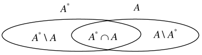
Figure 2: The set relationship.

In our algorithm, the AP does not know the number of its in-cell devices $K^{*}$. In this case, the algorithm output all the detected messages in $A$. Accordingly, we define the false alarm rate in this phase as

$$\begin{split}\frac{|A\backslash A^{*}|}{|A|},\end{split}$$ (100)

and the miss rate as

$$\begin{split}\frac{|A^{*}\backslash A|}{|A^{*}|}.\end{split}$$ (101)

The false alarm rate and miss rate reflect the error performance of the algorithm when the number of devices in the AP is unknown.

VI-B Simulation Parameter Setting

The detailed simulation parameters are listed in Table I. We consider a $500\times 500$ ${\rm m}^{2}$ rectangle where the devices are randomly distributed in the plane. According to [4], the number of devices on the plane with area 0.25 ${\rm km}^{2}$ can be up to $|\Phi|=2.5\times 10^{5}$, however, only a small part of them are active. In this paper, we consider the number of active devices $K$ ranges from 1000 to 8000, i.e., $K\in[1000,8000]$.

According to (12), we have $K^{*}\approx 1.11\times 10^{-2}K$ when $r=1$. And $K^{*}\approx 1.25\times 10^{-2}K$ when $r=16$. Assuming $K=1000$, we have $K^{*}\approx 11$ when $r=1$ and $K^{*}\approx 13$ when $r=16$. Assuming $K=8000$, we have $K^{*}\approx 89$ when $r=1$ and $K^{*}\approx 100$ when $r=16$. The AP aims to decode the messages transmitted by its neighbor, while the messages transmitted by its non-neighbor are treated as interference.

TABLE I: Simulation Parameters.

Parameters	Value
Channel gain threshold $\theta$	$10^{-6}$
Path-loss exponent $\alpha$	$4$
Transmit SNR of each device $\gamma$	60 dB
Average number of detected devices in each slot $K_{\rm max}$	$\left\lceil\frac{6K^{*}}{2^{p}}r^{\frac{1}{4}}\right\rceil$
The square area of the device distribution region $S$	$500\times 500\ {\rm m}^{2}$
Carrier spacing $\Delta f$	15 kHz
Maximum device delay $\tau_{\rm max}$	10 $\upmu$s

VI-C Synchronous Transmission

In this subsection, we set $\tau_{\rm max}=0$, i.e., the transmissions of different devices are synchronized. In this case, a state-of-the-art algorithm using RM codes is the list RM_LLD algorithm given in [29]. In [29], the author uses only the subset of the RM codewords; thus encodes fewer bits, namely $B=\frac{1}{2}(d+m+p)(d+m+p+1)$. Note that the algorithm proposed in [29] applies only for single antenna case. In our algorithm, we set $r=1,4,16$, respectively. For fair comparison, we set the codelength to be $C=2^{12}=4,096$ in both algorithms. In this case, the number of information bits in [29] is $B=\frac{1}{2}\times 12\times(12-1)=66$ bits. To make the transmit bits comparable, we set $d=0,m=10,p=2$ in our scheme. Since the number of slots is small, in our scheme, each messages randomly chooses one of the 4 slots for transmitting. Accordingly, the number of transmit bits of Algorithm 1 is $B=\frac{1}{2}m(m+3)+p=67$ bits, which is comparable with [29].

Fig. 3 illustrates the miss rate and false alarm rate of both algorithms. In Fig. 3, the horizontal axis is the number of neighbors of the AP $K^{*}$ and the total number of active devices $K$ when $r=1$, respectively. The author in [29] assume that the AP knows the number of its neighbors, thus the miss rate equals to the false alarm rate for the algorithm in [29]. In our algorithm, the AP does not need to know the number of its neighbors. Fig. 3 shows that the performance of Algorithm 1 improves as the number of receiving antennas increases. Fig. 3 demonstrates that Algorithm 1 outperforms the list RM_LLD algorithm when the number of active devices is larger than 2000. But the performance of the list RM_LLD algorithm is better when the number of active devices is smaller than 2000, i.e., the number of neighbors of the AP is less than 22. This is because the codelength in our algorithm is divided into 4 slots to reduce the number of active devices in each slot. However, when the number of active users is small (for example, below 2000), there is no need to use slotting. This suggests us that the number of slots should be reduced if the number of active devices is small. Fortunately, our algorithm can flexibly change the number of slots to deal with different situations.

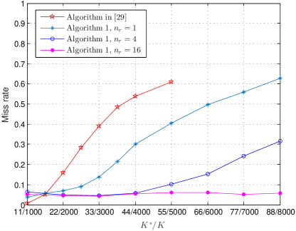
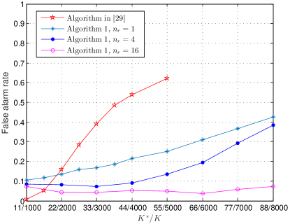
Figure 3: Performance comparison with the algorithm in [29]. (a) The miss rate and (b) the false alarm rate.

VI-D Asynchronous Transmission

In this subsection, we study the performance of Algorithm 1 under asynchronous transmission. The maximum delay is set to be $\tau_{\rm max}=10\ \upmu$s, further, the length of the cyclic prefix can be calculated as $M=\left\lceil\frac{3}{20}2^{m}\right\rceil$. We assume the normalized transmission delay $\Delta_{k}=2\pi\Delta f\tau_{k}$ is uniformly distributed in $[-\pi,\pi]$. As far as we know, this paper is the first using RM codes to handle continuous transmission delay in massive access.

Fig. 4 depicts the miss rate and false alarm rate obtained by Algorithm 1 with different number of receive antennas. We set $q=6,p=6,d=0$, which means that the number of slots and the length of each slot are both $2^{6}=64$ and $M=10$. In Fig. 4, the horizontal axis is $K^{*}$ and $K$ when $r=16$, respectively. In this case, the total number of information bits can be transmitted is $30$ bits according to (3), and the codelength is $2^{6}(2^{6}+10)=4,736$ according to (6).

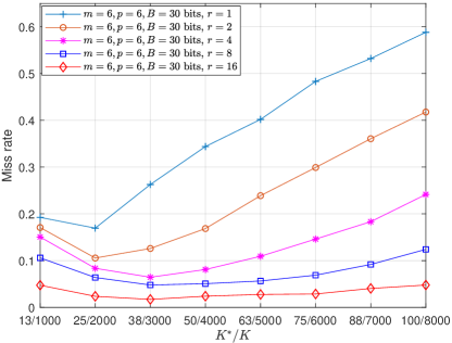
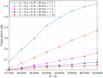
Figure 4: Performance comparison with different number of receiving antennas. (a) The miss rate and (b) the false alarm rate.

Fig. 4 shows that the performance of Algorithm 1 improves as the number of receiving antennas increases. If the number of receive antennas is increased from $r=1$ to $r=2$, the performance of Algorithm 1 will be greatly improved. However, if we further increase the number of receiving antennas, the increase of the performance is limited. Differently, we observe in Fig. 4 that the miss rate at $K=1000$ is greater than the miss rate at $K=2000$, which might appear surprising. We believe that this behavior is due to the suboptimal tuning of the parameters $\varepsilon$ and $K_{\rm max}$ in Algorithm 1. One of the advantage of Algorithm 1 is that no tuning of parameters is required. We use the same parameter choices throughout the paper. It is worth notice that both the miss rate and false alarm rate is below 0.05 when $r=16$. This indicates that we need use multiple antennas for practice use.

Fig. 5 shows the miss rate and false alarm rate versus the number of active devices with different number of information bits. The number of receive antennas is $r=16$ and $m+p=12$. For $d=0,1,2$, the number of sub-blocks is $1,2,4$, respectively, and the corresponding codelengths are $C=4,736,C=9,472$, and $C=18,944$, respectively. To patch the sub-blocks together, we add different number of parity check bits for different number of sub-blocks. These choices are made with a view of minimizing the number of bits devoted to parity check while keeping the probability of information loss in the patching process pretty low. We should emphasize that these choice are not optimal. Generally, the miss rate and the false alarm rate are related to the parity check bits. The more parity check bits, the worse the miss rate and the better the false alarm rate. We refer the reader to [55] for details of this method. Normally, the more information bits we transmit, the worse the error performance. For example, when the codelength is $18,944$, the error performance of the curve with $B=93$ bits is better than the curve with $B=121$ bits. Besides, the error performance of the curve with $B=30$ bits and $B=48$ bits are comparable, but the error performance of the curve with $B=93$ bits is much worse than that of the curve with $B=30$ bits and $B=48$ bits. This indicates two things: 1) because we need to append some parity check bits, even though we double the number of sub-blocks, the number of information bits will not double; 2) we find that only a small number of sub-blocks (up to 4) is beneficial. The error performance will be much worse if more than 4 sub-blocks are adopted, which is somewhat deviated from the implementation of using 11 sub-blocks in [54].

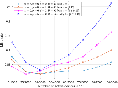
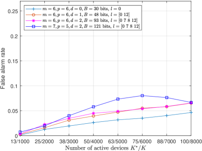
Figure 5: Performance comparison with different number of receiving antennas. (a) The miss rate and (b) the false alarm rate.

VII Conclusion

This paper has developed a new technique for asynchronous massive access using OFDM signaling and RM codes. The access points are assumed to have a large number of antennas. The proposed technique allows a flexible number of information bits and codelength. Numerical results demonstrate the effectiveness of the proposed technique as well as the gains due to a large number of antennas at the access points.

References

- [1] G. Durisi, T. Koch and P. Popovski, “Toward Massive, Ultrareliable, and Low-Latency Wireless Communication with Short Packets,” Proceedings of the IEEE, vol. 104, no. 9, pp. 1711-1726, Sept. 2016.
- [2] H. Tullberg, P. Popovski, Z. Li, M. A. Uusitalo, A. Hoglund, O. Bulakci, M. Fallgren and J. F. Monserrat, “The METIS 5G System Concept: Meeting the 5G Requirements,” IEEE Commun. Magazine, vol. 54, no. 12, pp. 132-139, December 2016.
- [3] L. Liu, E. G. Larsson, W. Yu, P. Popovski, C. Stefanovic and E. de Carvalho, “Sparse Signal Processing for Grant-Free Massive Connectivity: A Future Paradigm for Random Access Protocols in the Internet of Things,” IEEE Signal Processing Magazine, vol. 35, no. 5, pp. 88-99, Sept. 2018.
- [4] “IMT vision-Framework and overall objectives of the future development of IMT for 2020 and beyond,” Int. Telecommun. Union, Geneva, Switzerland, Recommendation ITU-R M.2083, Sep. 2015.
- [5] Y. Cai, Z. Qin, F. Cui, G. Y. Li and J. A. McCann, “Modulation and Multiple Access for 5G Networks,” IEEE Communications Surveys & Tutorials, vol. 20, no. 1, pp. 629-646, Firstquarter 2018.
- [6] X. Chen, T. Chen and D. Guo, “Capacity of Gaussian Many-Access Channels,” IEEE Trans. Inf. Theory, vol. 63, no. 6, pp. 3516-3539, June 2017.
- [7] X. Chen and D. Guo, “Many-access channels: The Gaussian case with random user activities,” in Proc. 2014 IEEE Int. Symp. Inf. Theory, Honolulu, HI, 2014, pp. 3127-3131.
- [8] A. Thompson and R. Calderbank, “Compressed Neighbour Discovery using Sparse Kerdock Matrices,” 2018 IEEE International Symposium on Information Theory (ISIT), Vail, CO, 2018, pp. 2286-2290.
- [9] L. Zhang and D. Guo, “Neighbor discovery in wireless networks using compressed sensing with Reed-Muller codes,” in Proc. 2011 Int. Symp. Modeling and Optimization of Mobile, Ad Hoc, and Wireless Netw., Princeton, NJ, 2011, pp. 154-160.
- [10] L. Zhang, J. Luo, and D. Guo, “Neighbor discovery for wireless networks via compressed sensing,” Perform. Eval., vol. 70, no. 7, pp. 457-471, 2013.
- [11] Z. Chen, F. Sohrabi and W. Yu, “Sparse Activity Detection for Massive Connectivity,” IEEE Trans. Signal Processing, vol. 66, no. 7, pp. 1890-1904, April, 2018.
- [12] L. Liu and W. Yu, “Massive Connectivity With Massive MIMO-Part I: Device Activity Detection and Channel Estimation,” IEEE Trans. Signal Processing, vol. 66, no. 11, pp. 2933-2946, June, 2018.
- [13] L. Liu and W. Yu, “Massive Connectivity With Massive MIMO-Part II: Achievable Rate Characterization,” IEEE Trans. Signal Processing, vol. 66, no. 11, pp. 2947-2959, June, 2018.
- [14] Z. Chen, F. Sohrabi and W. Yu, “Multi-Cell Sparse Activity Detection for Massive Random Access: Massive MIMO Versus Cooperative MIMO,” IEEE Trans. Wireless Commun., vol. 18, no. 8, pp. 4060-4074, Aug. 2019.
- [15] K. Senel and E. G. Larsson, “Grant-Free Massive MTC-Enabled Massive MIMO: A Compressive Sensing Approach,” IEEE Transactions on Communications, vol. 66, no. 12, pp. 6164-6175, Dec. 2018.
- [16] M. Ke, Z. Gao, Y. Wu, X. Gao and R. Schober, “Compressive Sensing-Based Adaptive Active User Detection and Channel Estimation: Massive Access Meets Massive MIMO,” IEEE Transactions on Signal Processing, vol. 68, pp. 764-779, 2020.
- [17] V. K. Amalladinne, K. R. Narayanan, J. Chamberland and D. Guo, “Asynchronous Neighbor Discovery Using Coupled Compressive Sensing,” 2019 IEEE International Conference on Acoustics, Speech and Signal Processing (ICASSP), Brighton, United Kingdom, 2019, pp. 4569-4573.
- [18] T. Jiang, Y. Shi, J. Zhang and K. B. Letaief, “Joint Activity Detection and Channel Estimation for IoT Networks: Phase Transition and Computation-Estimation Tradeoff,” IEEE Internet of Things Journal, vol. 6, no. 4, pp. 6212-6225, Aug. 2019.
- [19] J. Ahn, B. Shim, and K. B. Lee, “EP-based joint active user detection and channel estimation for massive machine-type communications,” IEEE Trans. Commun., vol. 67, no. 7, pp. 5178-5189, Jul. 2019.
- [20] X. Xu, X. Rao, and V. K. N. Lau, “Active user detection and channel estimation in uplink CRAN systems,” in Proc. Int. Conf. Commun., London, U.K., Jun. 2015, pp. 2727-2732.
- [21] X. Shao, X. Chen and R. Jia, “A Dimension Reduction-Based Joint Activity Detection and Channel Estimation Algorithm for Massive Access,” IEEE Trans. Signal Processing, vol. 68, pp. 420-435, 2020.
- [22] S. S. Kowshik, K. Andreev, A. Frolov and Y. Polyanskiy, “Energy efficient random access for the quasi-static fading MAC,” in 2019 IEEE Int. Symp. Inf. Theory (ISIT), Paris, France, 2019, pp. 2768-2772.
- [23] W. Cao, A. Dytso, Y. Shkel, G. Feng and H. V. Poor, “Sum-Capacity of the MIMO Many-Access Gaussian Noise Channel,” IEEE Trans. Commun., vol. 67, no. 8, pp. 5419-5433, Aug. 2019.
- [24] J. Ravi and T. Koch, “Capacity per Unit-Energy of Gaussian Many-Access Channels,” in Proc. 2019 IEEE Int. Symp. Inf. Theory (ISIT), Paris, France, 2019, pp. 2763-2767.
- [25] R. A. Chou and A. Yener, “The Degraded Gaussian Many-Access Wiretap Channel,” in Proc. 2019 IEEE Int. Symp. Inf. Theory (ISIT), Paris, France, 2019, pp. 672-676.
- [26] I. Zadik, Y. Polyanskiy and C. Thrampoulidis, “Improved bounds on Gaussian MAC and sparse regression via Gaussian inequalities,” in Proc. 2019 IEEE Int. Symp. Inf. Theory (ISIT), Paris, France, 2019, pp. 430-434.
- [27] S. D. Howard, A. R. Calderbank, and S. J. Searle, “A fast reconstruction algorithm for deterministic compressive sensing using second order Reed-Muller codes,” in Proc. 42nd Annu. Conf. Inf. Sci. Syst., Princeton, NJ, USA, 2008, pp. 11-15.
- [28] R. Calderbank, A. Thompson, “CHIRRUP: a practical algorithm for unsourced multiple access”, Information and Inference: A Journal of the IMA, December 2019.
- [29] J. Wang, Z. Zhang and L. Hanzo, “Joint Active User Detection and Channel Estimation in Massive Access Systems Exploiting Reed-Muller Sequences,” IEEE J. Select. Top. Sign. Proces., vol. 13, no. 3, pp. 739-752, June 2019.
- [30] H. Zhang, R. Li, J. Wang, Y. Chen and Z. Zhang, “Reed-Muller Sequences for 5G Grant-Free Massive Access,” in Proc. 2017 IEEE Global Commun. Conf., Singapore, 2017, pp. 1-7.
- [31] Q. Yu, H. Li, W. Meng and W. Xiang, “Sparse Code Multiple Access Asynchronous Uplink Multiuser Detection Algorithm,” IEEE Transactions on Vehicular Technology, vol. 68, no. 6, pp. 5557-5569, June 2019.
- [32] L. Applebaum, W. U. Bajwa, M. F. Duarte, and R. Calderbank, “Asynchronous code-division random access using convex optimization,” Physical Commun., vol. 5, no. 2, pp. 129-147, 2012.
- [33] K. Andreev, S. S. Kowshik, A. Frolov and Y. Polyanskiy, “Low Complexity Energy Efficient Random Access Scheme for the Asynchronous Fading MAC,” 2019 IEEE 90th Vehicular Technology Conference (VTC2019-Fall), Honolulu, HI, USA, 2019, pp. 1-5.
- [34] Xu Chen, Dongning Guo, and Gregory W. Wornell, “Sparse OFDM: A Compressive Sensing Approach to Asynchronous Neighbor Discovery,” arXiv preprint arXiv:1706.09387, 2017.
- [35] W. Zhu, M. Tao, X. Yuan and Y. Guan, “Deep-Learned Approximate Message Passing for Asynchronous Massive Connectivity,” IEEE Trans. Wireless Commun., vol. 20, no. 8, pp. 5434-5448, Aug. 2021.
- [36] H. F. Schepker, C. Bockelmann and A. Dekorsy, “Exploiting Sparsity in Channel and Data Estimation for Sporadic Multi-User Communication,” in Proc. 10th Int. Symp. Wireless Commun. Syst., Ilmenau, Germany, 2013, pp. 1-5.
- [37] J. Lee, G. T. Gil, and Y. H. Lee, “Channel estimation via orthogonal matching pursuit for hybrid MIMO systems in millimeter wave communications,” IEEE Trans. Commun., vol. 64, no. 6, 2370-2386, Jun. 2016.
- [38] H. Zhu and G. B. Giannakis, “Exploiting Sparse User Activity in Multiuser Detection,” IEEE Trans. Commun., vol. 59, no. 2, pp. 454-465, February 2011.
- [39] B. Shim and B. Song, “Multiuser detection via compressive sensing,” IEEE Commun. Lett., vol. 16, no. 7, pp. 972-974, Jul. 2012.
- [40] B. Wang, L. Dai, T. Mir, and Z. Wang, “Joint user activity and data detection based on structured compressive sensing for noma,” IEEE Commun. Lett., vol. 20, no. 7, pp. 1473-1476, Jul. 2016.
- [41] B. K. Jeong, B. Shim, and K. B. Lee, “MAP-based active user and data detection for massive machine-type communications,” IEEE Trans. Veh. Technol., vol. 67, no. 9, pp. 8481-8494, Sep. 2018.
- [42] E. Paolini, G. Liva and M. Chiani, “Coded Slotted ALOHA: A Graph-Based Method for Uncoordinated Multiple Access,” IEEE Trans. Inf. Theory, vol. 61, no. 12, pp. 6815-6832, Dec. 2015.
- [43] E. Casini, R. De Gaudenzi and O. Del Rio Herrero, “Contention Resolution Diversity Slotted ALOHA (CRDSA): An Enhanced Random Access Scheme for Satellite Access Packet Networks,” IEEE Trans. Wireless Commun., vol. 6, no. 4, pp. 1408-1419, April 2007.
- [44] R. De Gaudenzi, O. del Río Herrero, G. Acar and E. Garrido Barrabés, “Asynchronous Contention Resolution Diversity ALOHA: Making CRDSA Truly Asynchronous,” IEEE Transactions on Wireless Communications, vol. 13, no. 11, pp. 6193-6206, Nov. 2014.
- [45] E. Sandgren, A. Graell i Amat and F. Brännström, “On Frame Asynchronous Coded Slotted ALOHA: Asymptotic, Finite Length, and Delay Analysis,” IEEE Transactions on Communications, vol. 65, no. 2, pp. 691-704, Feb. 2017.
- [46] O. Ordentlich and Y. Polyanskiy, “Low complexity schemes for the random access Gaussian channel,” in 2017 IEEE Int. Symp. Inf. Theory (ISIT), Aachen, 2017, pp. 2528-2532.
- [47] A. Vem, K. R. Narayanan, J. Cheng and J. Chamberland, “A user-independent serial interference cancellation based coding scheme for the unsourced random access Gaussian channel,” in Proc. IEEE Inf. Theory Workshop (ITW), Kaohsiung, 2017, pp. 121-125.
- [48] S. S. Kowshik and Y. Polyanskiy, “Quasi-static fading MAC with many users and finite payload,” in Proc. 2019 IEEE Int. Symp. Inf. Theory (ISIT), Paris, France, 2019, pp. 440-444.
- [49] P. Yang, D. Guo, and H. Yang, “Massive Access in Multi-cell Wireless Networks Using Reed-Muller Codes,” arXiv preprint arXiv:2003.11568, 2020.
- [50] H. Han, Y. Li and X. Guo, “A Graph-Based Random Access Protocol for Crowded Massive MIMO Systems,” IEEE Transactions on Wireless Communications, vol. 16, no. 11, pp. 7348-7361, Nov. 2017.
- [51] E. Björnson, E. de Carvalho, J. H. Sørensen, E. G. Larsson and P. Popovski, “A Random Access Protocol for Pilot Allocation in Crowded Massive MIMO Systems,” IEEE Transactions on Wireless Communications, vol. 16, no. 4, pp. 2220-2234, April 2017.
- [52] Y. Han, B. D. Rao and J. Lee, “Massive Uncoordinated Access With Massive MIMO: A Dictionary Learning Approach,” IEEE Transactions on Wireless Communications, vol. 19, no. 2, pp. 1320-1332, Feb. 2020.
- [53] L. Zhang and D. Guo, “Virtual Full Duplex Wireless Broadcasting via Compressed Sensing,” IEEE/ACM Transactions on Networking, vol. 22, no. 5, pp. 1659-1671, Oct. 2014.
- [54] V. K. Amalladinne, A. Vem, D. K. Soma, K. R. Narayanan and J. Chamberland, “A Coupled Compressive Sensing Scheme for Unsourced Multiple Access” in Proc. 2018 IEEE International Conference on Acoustics, Speech and Signal Processing (ICASSP), Calgary, AB, 2018, pp. 6628-6632.
- [55] V. K. Amalladinne and J. Chamberland and K. R. Narayanan, “A Coded Compressed Sensing Scheme for Uncoordinated Multiple Access,” arXiv preprint arXiv:1809.04745, 2018.