Symbolic Brittleness in Sequence Models:
on Systematic Generalization in Symbolic Mathematics

Abstract

Neural sequence models trained with maximum likelihood estimation have led to breakthroughs in many tasks, where success is defined by the gap between training and test performance. However, their ability to achieve stronger forms of generalization remains unclear. We consider the problem of symbolic mathematical integration, as it requires generalizing systematically beyond the test set. We develop a methodology for evaluating generalization that takes advantage of the problem domain’s structure and access to a verifier. Despite promising in-distribution performance of sequence-to-sequence models in this domain, we demonstrate challenges in achieving robustness, compositionality, and out-of-distribution generalization, through both carefully constructed manual test suites and a genetic algorithm that automatically finds large collections of failures in a controllable manner. Our investigation highlights the difficulty of generalizing well with the predominant modeling and learning approach, and the importance of evaluating beyond the test set, across different aspects of generalization.

1 Introduction

Despite their success, recent studies reveal undesirable properties of conventional neural sequence models, such as assigning high-probabilities to unrealistic sequences (Holtzman et al. 2020; Welleck et al. 2020), susceptibility to adversarial attacks (Wallace et al. 2019), and limited generalization on symbolic tasks (Saxton et al. 2019; Nogueira, Jiang, and Li 2021), even with very large models and datasets (Henighan et al. 2020). Despite these drawbacks, Lample and Charton (2019) recently demonstrated that a standard sequence-to-sequence model, which we call a neural sequence integrator, performs surprisingly well at symbolic integration, solving problems that are beyond traditional symbolic solvers and achieving near perfect test accuracy.

Input	Integral	Prediction
$30\cos(39x)$	$\frac{10}{13}\sin(39x)$	$\frac{10}{13}\sin(39x)$	✓
$17\cos(83x)$	$\frac{17}{83}\sin(83x)$	${\color[rgb]{1,0,0}{\frac{1}{17}}\sin(83x)}$	✗
$34\cos(77x)$	$\frac{34}{77}\sin(77x)$	${\color[rgb]{1,0,0}\sin(77x)}$	✗
$x^{209}$	$\frac{1}{210}x^{210}$	$\frac{1}{210}x^{210}$	✓
$x^{764}$	$\frac{1}{765}x^{765}$	$\frac{1}{765}x^{765}$	✓
$x^{209}+x^{764}$	$\frac{1}{210}x^{210}+\frac{1}{765}x^{765}$	${\color[rgb]{1,0,0}{\frac{1}{205}x^{205}}}$	✗
$-241$	$-241x$	${\color[rgb]{1,0,0}{-239x}}-14400$	✗
$123^{x}$	$\frac{123^{x}}{\log(123)}$	${\color[rgb]{1,0,0}{\frac{123^{x}}{1+\log(123)}}}$	✗
$4^{x}+x^{465}+1$	$\frac{x^{466}}{466}+x+\frac{4^{x}}{\log(4)}$	$\frac{x^{466}}{466}+x+{\color[rgb]{1,0,0}{e^{x}}}$	✗

Table 1: Despite its impressive ability to integrate equations that are out of reach for traditional symbolic solvers, the neural sequence integrator shows deficiences in robustness (top) and compositionality (middle), and fails on adversarial problems discovered by SAGGA (bottom).

Recent studies suggest that achieving strong and systematic generalization is difficult with vanilla sequence-to-sequence methods, as they latch onto regularities in the training data, learning dataset-specific solutions that do not generalize beyond the training distribution (e.g. Agrawal, Batra, and Parikh (2016); Lake and Baroni (2018); Bahdanau et al. (2019); Hupkes et al. (2020)). Symbolic integration – finding the integral of a mathematical function – specifically requires these forms of generalization, as it involves an underlying structure that extends beyond this fixed training distribution. For instance, the rule $\int k=kx+C$ applies to all constants $k$, and the sum rule $\int f_{1}+\int f_{2}=\int(f_{1}+f_{2})$ means that integrating two functions correctly should imply integrating their sum correctly. Symbolic integration also offers a structured problem domain and a verifier for evaluating whether a proposed solution is correct, making it an effective setting for evaluating generalization. As the neural sequence integrator relies on a common recipe– a large-scale transformer trained to maximize the likelihood of a training set of input-output sequences – it is especially interesting to study whether it generalizes systematically.

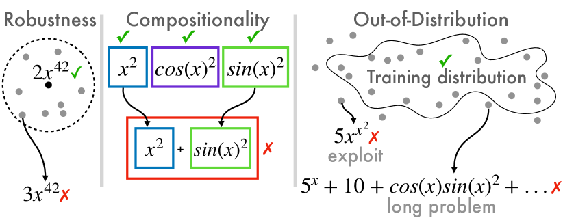
Figure 1: Illustrating robustness, compositionality, and out-of-distribution deficiencies in the neural sequence integrator.

In this paper, we find a discrepancy between the traditional notion of generalization captured by test set accuracy and the generalization needed in symbolic mathematics. While the model’s test accuracy is nearly perfect, we find this breaks down when testing its robustness, compositionality, and out-of-distribution generalization (e.g. Table 1). We describe a methodology for evaluating these aspects, by constructing problem sets and developing a genetic algorithm, SAGGA (Symbolic Archive Generator with Genetic Algorithms), that automatically discovers diverse and targeted failures. We find that successfully integrating an in-distribution problem does not imply success on nearby problems, despite being governed by the same underlying rule (robustness). Moreover, the model often succeeds on a collection of problems without being able to systematically compose those problems (compositionality), and struggles to generalize to longer problems, larger values, and functions not covered in training (out-of-distribution).

In addition to the model’s approximate mode being incorrect – i.e. the most probable sequence returned by beam search – the deficiencies are present deeper into its ranked list of candidate solutions, impacting the model’s effectiveness in a search-and-verify setting. Overall, our investigation highlights the difficulty of achieving robustness, compositionality, and out-of-distribution generalization with the predominant modeling and learning approach, and the importance of evaluating beyond the test set, across aspects of generalization that are required by the task at hand.

2 Problem Setup

Symbolic integration is the problem of finding the integral $\mathbf{y}$ of an input equation $\mathbf{x}$. For instance, $x^{2}/2$ is the integral of $x$, up to an additive constant.

Neural sequence integrator.

Lample and Charton (2019) frame symbolic integration as a sequence-to-sequence problem. In this view, input and output equations $\mathbf{x}$ and $\mathbf{y}$ are prefix-notation sequences. The neural sequence integrator uses a 6-layer transformer (Vaswani et al. 2017) to model the distribution $p_{\theta}(\mathbf{y}|\mathbf{x})=\prod_{t=1}^{T_{\mathbf{y}}}p_{\theta}(y_{t}|y_{<t},\mathbf{x})$ by training the model to maximize the log-likelihood of a set of training problems, $\arg\max_{\theta}\sum_{(\mathbf{x},\mathbf{y})\in\mathcal{D}}\log p_{\theta}(\mathbf{y}|\mathbf{x})$. Given a trained model and input $\mathbf{x}$, a set of predicted solutions ranked by a model score is obtained by beam search, denoted $\{\hat{}\mathbf{y}_{1},\ldots,\hat{}\mathbf{y}_{k}\}=f_{\theta}(\mathbf{x};k,b)$, where $b$ is beam size and $k$ is the number of candidates saved for evaluation. For brevity we omit $b$ in the discussion unless necessary.

Evaluation.

The standard practice is to evaluate a candidate $\hat{}\mathbf{y}$ by checking whether the derivative of $\hat{}\mathbf{y}$ is equivalent to $\mathbf{x}$ using a symbolic solver (e.g. Sympy). In the maximum-a-posteriori (MAP) setting, the model’s output is considered correct if its top-ranked candidate $\hat{}\mathbf{y}_{1}$ is correct. This criterion is relaxed in the search-and-verify setting, where the model’s output is considered correct if any of its $k$ candidates $\{\hat{}\mathbf{y}_{1},\ldots,\hat{}\mathbf{y}_{k}\}$ is correct. In this view, the neural network narrows the search space to a small set of candidates that are checked, trading off correctness for search and verification cost. We denote checking $k$ candidate solutions as,

$$m(\mathbf{x},f_{\theta}(\mathbf{x};k)) =\begin{cases}0&\mathbf{x}\equiv\frac{d}{dx}\hat{}\mathbf{y}_{i}\text{ for any }i\in 1\text{ to }k,\\ 1&\text{otherwise}.\end{cases}$$ (1)

In other words, $m(\cdot,\cdot)$ is 1 when the model fails to predict the correct integral, and 0 when the model succeeds. We measure the proportion of failures on problems $X=\{\mathbf{x}_{1},\ldots,\mathbf{x}_{N}\}$ using $k$ candidate solutions per problem as:

$$\texttt{Fail@k}(f_{\theta},X)=\frac{1}{N}\sum_{\mathbf{x}\in X}m(\mathbf{x},f_{\theta}(\mathbf{x};k)).$$ (2)

Fail@k is 0 when the model correctly integrates all of the problems in $X$, and increases towards 1 as it fails to integrate more problems. Evaluating a model’s performance in the MAP setting corresponds to evaluating Fail@1, while the search-and-verify setting with a budget of $k>1$ candidates uses Fail@k. We omit $k$ in $f_{\theta}(\mathbf{x};k)$ unless necessary.

2.1 Experiment Structure

We structure our investigation into three parts (Figure 1). We begin close to the model’s training distribution, evaluating robustness to small perturbations of in-distribution problems and simple functions. We then ask whether learning to integrate a collection of functions implies that the model can integrate a composition of those functions. Finally we depart from the training distribution by studying extrapolation to larger problems and values, then by finding adversarial exploits that expose gaps in the training distribution.

Experimental setup.

We use the implementation and pre-trained model from Lample and Charton (2019) for all of our experiments, specifically the FWD+BWD+IBP model which obtained top-10 accuracies of 95.6%, 99.5%, and 99.6% on their publicly available test sets. Our evaluation is based on their code, we use their utilities for inputs and outputs, and by default use beam search with beam-size 10. Following the authors, we use Sympy to check whether the derivative of a prediction is equal to the original problem. We generously count the prediction as correct if a timeout occurs. See the Apppendix for additional details.

2.2 Automatic Problem Discovery with SAGGA

Automatically finding problems that expose deficiencies requires a non-differentiable cost (Equation 1), satisfying constraints for valid equations, and finding diverse problem sets to characterize each aspect of generalization. To address these challenges, we develop SAGGA (Symbolic Archive Generation with Genetic Algorithms), a gradient-free genetic algorithm which iteratively finds diverse failures.

At each iteration, SAGGA mutates a seed set of problems by modifying each problem’s equation tree, ensuring that the resulting candidates are valid equations. The candidates are scored by a fitness function – i.e. according to whether the neural sequence integrator fails to integrate the problem and other desired constraints – and the highest-fitness candidates are saved in a problem archive. The next seed set is then formed to balance diversity and fitness, by clustering candidates and selecting the highest-fitness members of each cluster. SAGGA continues until the archive contains a target number of problems. Algorithm 1 summarizes SAGGA.

SAGGA offers control over the types of problems that it discovers through its seed problems, fitness function, and mutation strategy. We detail our choices for each kind of generalization in their respective sections, and show default settings and further implementation details in the Appendix.

Parameters: Fitness $F(f_{\theta},\mathbf{x})\rightarrow\mathbb{R}$,

mutate and seed strategies, archive size $N$.

Output: Problem archive $\mathcal{D}=\{\mathbf{x}_{1},\ldots,\mathbf{x}_{N}\}$.

$\mathcal{D}=\emptyset$

  // initial archive

$\hat{\mathbf{x}}^{(0)}_{1:M}=\texttt{seed}(\mathcal{D},\emptyset)$

  // initial seed

while $|\mathcal{D}|<N$ do

      

       // generate mutations

       $\tilde{}\mathbf{x}_{1:M^{\prime}}^{(i)}=\texttt{mutate}(\hat{\mathbf{x}}^{(i)}_{1:M})$

      

       // select problems by fitness

       $\mathbf{x}_{1:M^{\prime\prime}}^{(i)}=\texttt{select}(F,\tilde{}\mathbf{x}_{1:M^{\prime}}^{(i)})$

      

       // archive selected problems

       $\mathcal{D}=\mathcal{D}\cup\mathbf{x}_{1:M^{\prime\prime}}^{(i)}$

      

       // choose next seed

       $\hat{\mathbf{x}}^{(i+1)}_{1:M}=\texttt{seed}(\mathcal{D},F,\tilde{}\mathbf{x}_{1:M^{\prime}}^{(i)})$

Algorithm 1 SAGGA. Each seed problem denoted as $\hat{}\mathbf{x}$, mutated problem as $\tilde{}\mathbf{x}$, archived problem as $\mathbf{x}$.

3 Robust or Brittle?

First, we study whether the model’s strong test-set performance adequately represents its robustness. Robustness tells us whether the integration model systematically solves all problems in a neighborhood governed by a generalizable pattern; for instance a model that solves $\int 26x^{42}$ should solve $\int 53x^{42}$. We study problems that are nearby to those from the original test distribution, as well as to simple primitive functions that offer fine-grained, interpretable control.

A robust model is stable to small perturbations in input, meaning that it gets nearby problems $\tilde{\mathbf{x}}$ correct when it gets a problem $\mathbf{x}$ correct. Formally, let $X=\{\mathbf{x}_{1},\ldots,\mathbf{x}_{N}\}$ contain problems that the model gets correct, $\sum_{\mathbf{x}\in X}m(\mathbf{x},f_{\theta}(\mathbf{x}))=0,$ and let $\mathcal{N}_{d}(\mathbf{x})$ be a set of problems that are nearby to $\mathbf{x}$ according to a distance $d(\mathbf{x},\tilde{\mathbf{x}})$. We measure robustness by measuring failures on nearby problems,

$$\texttt{Fail@k}(f_{\theta},X_{\mathcal{N}}),$$ (3)

where $X_{\mathcal{N}}=\bigcup_{\mathbf{x}\in X}\mathcal{N}_{d}(\mathbf{x})$. We measure this quantity by varying (i) the neighborhood $\mathcal{N}_{d}(\mathbf{x})$ used to generate nearby problems, and (ii) the seed problems $X$ to consider. Below, we will refer to a problem as $\mathbf{x}$ or $f$ interchangeably.

Type	Test	Fail@50	Fail@10	Fail@1
coeff	$k_{1}\ln(k_{2}x)$	0.0	0.0	0.0
	$k_{1}x$	0.0	0.0	0.0
	$k_{1}x^{42}$	0.0	6.1	45.5
	$k_{1}\exp(k_{2}x)$	15.4	20.8	30.3
	$k_{1}\sin(k_{2}x)$	6.6	19.6	29.7
	$k_{1}\cos(k_{2}x)$	10.6	20.7	28.2
	$k_{1}\tan(k_{2}x)$	13.9	17.4	24.2
coeff	$1/k\cdot f$	5.9	12.0	13.7
coeff	$k\cdot f$	5.4	5.8	16.3
+exp	$f+e^{x}$	0.9	1.6	3.3
+ln	$f+\ln(x)$	1.9	3.2	5.3

Table 2: Robustness results with simple primitives (top) and validation problems $f$ which the model correctly integrates (bottom). Coefficients are sampled from [1, 100].

Input	Integral	Prediction
$30\cos(39x)$	$\frac{10}{13}\sin(39x)$	$\frac{10}{13}\sin(39x)$	✓
$17\cos(83x)$	$\frac{17}{83}\sin(83x)$	${\color[rgb]{1,0,0}{\frac{1}{17}}\sin(83x)}$	✗
$34\cos(77x)$	$\frac{34}{77}\sin(77x)$	${\color[rgb]{1,0,0}\sin(77x)}$	✗
$26x^{42}$	$\frac{26}{43}x^{43}$	$\frac{26}{43}x^{43}$	✓
$88x^{42}$	$\frac{88}{43}x^{43}$	${\color[rgb]{1,0,0}8x^{43}}$	✗
$53x^{42}$	$\frac{53}{43}x^{43}$	${\color[rgb]{1,0,0}(x^{44}+x)/x}$	✗

Table 3: Robustness examples. We show the model’s top prediction (beam search, size 10). Note that $(x^{44}+x)/x=x^{43}+1$; its derivative is $43x^{42}$ and is hence incorrect.

3.1 Manually Testing Robustness

To define nearby problems, we first consider manual templates which minimally perturb a problem $f$, e.g.

$$k\cdot f,\quad f+\ln x,\quad\ldots$$

These problems are nearby $f$ in the sense that a single operation is added to the problem’s equation tree, or a small number of node values are changed in the tree.

Brittleness on simple primitive functions.

We first investigate whether the neural sequence integrator is robust on simple primitive functions, since they make up more complicated functions and are frequently entered by real-world users. We use a manual neighborhood which yields,

$$X_{\mathcal{N}}=\{ k_{1}\ln(k_{2}x),\quad k_{1}\exp(k_{2}x),\quad k_{1}x,\quad k_{1}x^{42},$$

$$k_{1}\sin(k_{2}x),\quad k_{1}\cos(k_{2}x),\quad k_{1}\tan(k_{2}x)\},$$

where $k_{1}\sim\mathcal{U}(a,b)$ and $k_{2}\sim\mathcal{U}(a,b)$ are randomly sampled coefficients from a range $(a,b)$. We use $[0,100]$ which is covered by the training distribution and evaluate on 1,000 $k_{1},k_{2}$ pairs sampled without replacement for each primitive.

Table 2 shows the results. On a positive note, the neural sequence integrator is robust on the primitives $k_{1}x$ and $k_{1}\ln(k_{2}x)$. The integral of $k_{1}x$ is $\frac{k_{1}}{2}x^{2}$, so the model learned to divide by 2 for these cases. The integral of $\ln$ involves copying the coefficients into a correct template (that is, $\int k_{1}\ln(k_{2}x)=k_{1}x(\ln(k_{2}x)-1)$), and the neural sequence integrator learned this behavior.

On the other hand, the model is surprisingly brittle on the other primitives. These require dividing coefficients (e.g. $\int k_{1}\cos(k_{2}x)=\frac{k_{1}}{k_{2}}\sin(k_{2}x)$). The failure rate shows that the model has not perfectly learned the required division behavior. Moreover, despite learning a ‘division by 2’ rule for integrating $k_{1}x$, the neural sequence integrator’s failures on $k_{1}x^{42}$ indicate that it did not perfectly learn an analogous ‘division by 43’ rule. Table 3 shows examples.

Test accuracy does not imply robustness.

Next, we want to see whether the neural sequence integrator’s strong test accuracy implies that it is robust on test problems. We use the validation set, and perturb validation problems that the model correctly integrates using the neighborhoods,

$$X_{\mathcal{N}_{1}}=\{ \frac{1}{k}f,\quad k\cdot f\},\quad X_{\mathcal{N}_{2}}=\{f+e^{x},\quad f+\ln(x)\},$$

where $k\sim\mathcal{U}(1,100)$. The first set multiplies the function by a constant, while the second adds a single primitive.

Table 2 shows the results. Despite achieving perfect accuracy on the original problems, the model frequently fails under the slight perturbations. The local neighborhood around validation examples reveals deficiencies in robustness that are not evident from validation performance alone, aligning with findings in NLP tasks (Gardner et al. 2020).

3.2 Automatically Finding Robustness Failures

Next, we use SAGGA to automatically discover robustness failures in the neighborhood of a seed set of problems.

Discovering brittleness near simple problems.

First, we run SAGGA and only allow it to mutate leaves in a problem’s equation tree into a random integer. The problems are nearby in the sense that the tree’s structure is not changing, only a small number of its leaf values. We use SAGGA to mutate the leaves of seed sets of 9 polynomials $X_{\texttt{poly}}$ and 9 trigonometric functions $X_{\texttt{trig}}$, which are listed in the Appendix. We run SAGGA until it discovers 1000 failing problems, then cluster these using k-means on SciBERT embeddings (Beltagy, Lo, and Cohan 2019) of each problem.

Table 4 shows three members from three discovered problem clusters, for the polynomial and trigonometric seeds. Intuitively, each cluster shows failures in a neighborhood around a prototypical problem – for instance, on $2x^{42}+\textbf{k}$ the neural sequence integrator correctly integrates $2x^{42}+\textbf{21}$, but not the problems in Cluster 2 (e.g. $2x^{42}+\textbf{22}$). See Appendix Table 16 for more prototypes and the model’s predictions.

Curiously, each problem in a neighborhood is governed by a common template – e.g. the problems $\{-104,-136,-33\}$ are governed by $\int k=kx+C$, yet the failures suggest that the neural sequence integrator has either not inferred the template, or does not apply it across the neighborhood. To investigate this phenomenon, we show the raw model prediction in Table 5, along with its simplified version and derivative. Compared to the underlying template $\int k=kx+C$ the model’s raw output is long and complex. In contrast, the simplified version is short; we hypothesize this gap makes adhering to the template difficult.

Seed	Cluster 1	Cluster 2	Cluster 3
$X_{\texttt{poly}}$	$-104$	$2x^{42}+22$	$-47+2/x-2/x^{71}$
	$-136$	$2x^{42}+28$	$-47+2/x-31/x^{71}$
	$-33$	$2x^{42}+68$	$-71+36/x+2/x^{71}$
$X_{\texttt{trig}}$	$13\cos{19x}$	$13\cos{83x}-59$	$10\sin{47x}\cos{2x}$
	$13\cos{83x}$	$17\cos{37x}-49$	$10\sin{90x}\cos{2x}$
	$17\cos{47x}$	$17\cos{41x}-45$	$19\sin{90x}\cos{2x}$

Table 4: Example robustness problems discovered by SAGGA which the neural sequence integrator fails to integrate. See Appendix Table 16 for model predictions.

$\mathbf{x}$	Raw	Simplified	Deriv.
$-104$	$x^{2}+2x-(x+25)^{2}$	$-48x-625$	$-48$
$-136$	$x^{2}-x(x+130)+2x$	$-128x$	$-128$
$-33$	$x^{2}+x-(x+16)^{2}$	$-31x-256$	$-31$

Table 5: The raw model predictions for the problems $\mathbf{x}$ and their simplified forms. Each prediction is incorrect since its derivative is not equal to $\mathbf{x}$. The neural sequence integrator’s raw output is long and varied compared to the underlying integration rule $\int k=kx+C$.

Discovering brittleness near validation problems.

Finally, we use SAGGA to discover difficult problems that are close to a target set $X$ – in our case validation problems – according to an explicit distance $d(\mathbf{x},\tilde{\mathbf{x}})$. This allows for less hand-designing of the perturbations.

Specifically, we define a fitness which is high whenever a candidate is close to any problem in a target set $X$,

$$\text{fitness}(\mathbf{\tilde{x}}) =\left[\min_{\mathbf{x}\in X}d(\mathbf{x},\mathbf{\tilde{x}})\right]^{-1}\cdot m(\tilde{\mathbf{x}},f_{\theta}(\mathbf{\tilde{x}})).$$ (4)

We randomly sample 10 validation problems to form $X$, set SAGGA’s initial seed to $X$, and use cosine similarity of SciBERT vectors to define the distance $d(\mathbf{x},\tilde{\mathbf{x}})$. Since the distance now constrains the problems, we are free to use a wider set of mutations: changing a node’s operation, adding an argument to a node, and replacing the node with a random constant, symbol, or simple operation.

Table 6 shows example problems that SAGGA discovers around the successful validation problems, exposing a wider class of robustness failures than our preceding experiments.

Validation Problem	Nearby Failures
$-x^{2}+x+\log(4)\tan(x)$	$-x^{2}+x+\log(4)\tan(17x^{2})$
	$-x^{2}+x+\log(4)\tan(2x^{2})$
	$-x^{2}+x+\log(4)\tan(63/x^{2})$
$\sqrt{3x+3}-2$	$\sqrt{-86^{x^{2}}+62/x}-40$
	$\sqrt{14+62/x}+4$
	$\sqrt{14+62/x}-2$
$\tan(\exp(2))/18x$	$\tan(\exp(2+71/x))/18x$
	$\tan(\exp(2-46^{x}))/18x$
	$\tan(\exp(37x))/18x$

Table 6: SAGGA discovers failures around successful validation problems, within a neighborhood defined by an explicit distance. Model predictions are in Appendix Table 16.

4 Integrating Parts But Not The Whole

While the preceding section identified weaknesses in robustness – for instance, integrating $26x^{42}$ but not $88x^{42}$ – a remaining question is whether successfully integrating a collection of primitives implies that a composition of those primitives will be successfully integrated.

Compositionality refers to forming compound equations from known primitives and operations. A compositional model should correctly integrate equations of the form,

$$f=f_{1}\circ f_{2}\circ\cdots\circ f_{k},$$ (5)

where $f_{1},\ldots,f_{k}$ are equations that the model successfully integrates, and $\circ$ is a binary operation (e.g. addition). For instance, a system that integrates $x^{2}$ and $\cos x$ and is capable of addition should successfully integrate $x^{2}+\cos x$.

Formally, we say that a model is $k$-compositional with respect to equations $X$ and operation $\circ$ when it successfully integrates any combination of $k$ equations from $X$, $\sum_{\mathbf{x}\in\tilde{X}}m(\mathbf{x},f_{\theta}(\mathbf{x}))=0$, where $\tilde{X}=\{f_{1}\circ\cdots\circ f_{k}|f_{i}\in X\}$.

We evaluate $k$-compositionality with respect to addition, using simple primitive functions and validation problems. As integration is linear, $\int(f+g)=\int f+\int g$, compositionality with respect to addition is a reasonable requirement.

Input	Prediction
$x^{1/3}$	$\frac{3}{4}x^{4/3}$	✓
$x^{1/606}$	$\frac{606}{607}x^{\frac{607}{606}}$	✓
$x^{1/3}+x^{1/606}$	${\color[rgb]{1,0,0}{\frac{3}{5}x^{\frac{5}{3}}+\frac{6}{613}x^{\frac{613}{606}}}}$	✗
$x^{209}$	$\frac{1}{210}x^{210}$	✓
$x^{764}$	$\frac{1}{765}x^{765}$	✓
$x^{209}+x^{764}$	${\color[rgb]{1,0,0}{\frac{1}{205}x^{205}}}$	✗
$14\cos(58x)$	$\frac{7}{29}\sin(58x)$	✓
$46\cos(84x)$	$\frac{23}{42}\sin(84x)$	✓
$14\cos(58x)+46\cos(84x)$	${\color[rgb]{1,0,0}{\sin(59x)\cos(x)}}$	✗

Table 7: Compositionality examples. We show the model’s top prediction (beam search, width 10). The model successfully integrates the individual primitives, but not their sum.

Type	Test	Fail@50	Fail@10	Fail@1
exp(1)	$f_{1}$	00.0	00.0	00.0
exp(2)	$f_{1}+f_{2}$	70.8	72.4	84.9
exp(3)	$f_{1}+f_{2}+f_{3}$	91.3	97.5	99.5
exp(4)	$f_{1}+\ldots+f_{4}$	86.2	97.4	99.8
coeff(1)	$f_{1}$	00.0	00.0	00.0
coeff(2)	$f_{1}+f_{2}$	8.60	16.2	29.2
coeff(3)	$f_{1}+f_{2}+f_{3}$	23.8	37.5	61.0
coeff(4)	$f_{1}+\ldots+f_{4}$	23.1	38.7	60.0
valid(1)	$f_{1}$	00.0	00.0	00.0
valid(2)	$f_{1}+f_{2}$	6.80	14.5	15.0
valid(3)	$f_{1}+f_{2}+f_{3}$	21.5	36.5	43.6
valid(4)	$f_{1}+\ldots+f_{4}$	52.5	69.0	79.2

Table 8: Compositionality. Top: successful simple primitives from the robustness experiments (Table 2). Bottom: successful validation-set primitives. Despite integrating each primitive, the model struggles to integrate their sums.

Succeeding on simple primitives, failing on their sum.

We collect simple primitives from the coefficient robustness experiments that the model successfully integrates (coeff), and successful exponents $x^{c}$ or $x^{1/c}$, $c\in[0,1000]$ (exp). We randomly sample 1000 compound equations $f_{1}+\ldots+f_{k}$ for $k\in\{2,3,4\}$ and evaluate the failure rate. Table 8 shows the results. Adding two primitives gives failure rates of 29% and 85% for coefficient and exponent primitives, respectively, despite failing 0% of the time on the individual primitives. As the number of compositions increases, the failure rate increases towards 100%. Table 7 shows examples.

Succeeding on test problems, failing on their sum.

We perform a similar experiment using successful validation-set functions. We filter examples longer than 20 tokens so that composed equations are within the training domain in terms of length, and sample 1000 compound equations $f_{1}+\ldots+f_{k}$ for $k\in\{2,3,4\}$. As seen in Table 8, the failure rate grows as the number of compositions increases, similar to the simple primitives case. Maximizing the likelihood of a large training set did not yield a compositional model.

5 Departing Further From Training

The preceding experiments found problems that were nearby to, or composed directly from, in-distribution examples. In this section, we deliberately move from the model’s training distribution to evaluate its out-of-distribution generalization. First, we study extrapolation to longer equation sizes than those in its training distribution, and to integer ranges that are only sparsely covered in the training set. Then we use SAGGA to expose exotic failures and reveal problem classes that were not covered during training.

Nodes	Fail@10	Fail@1
1-15	0.4	1.6
20	1.9	10.7
25	7.2	17.2
30	24.4	37.1
35	49.0	59.2

Table 9: Extrapolation to more operator nodes under the training data generation process. Training used 1-15 nodes.

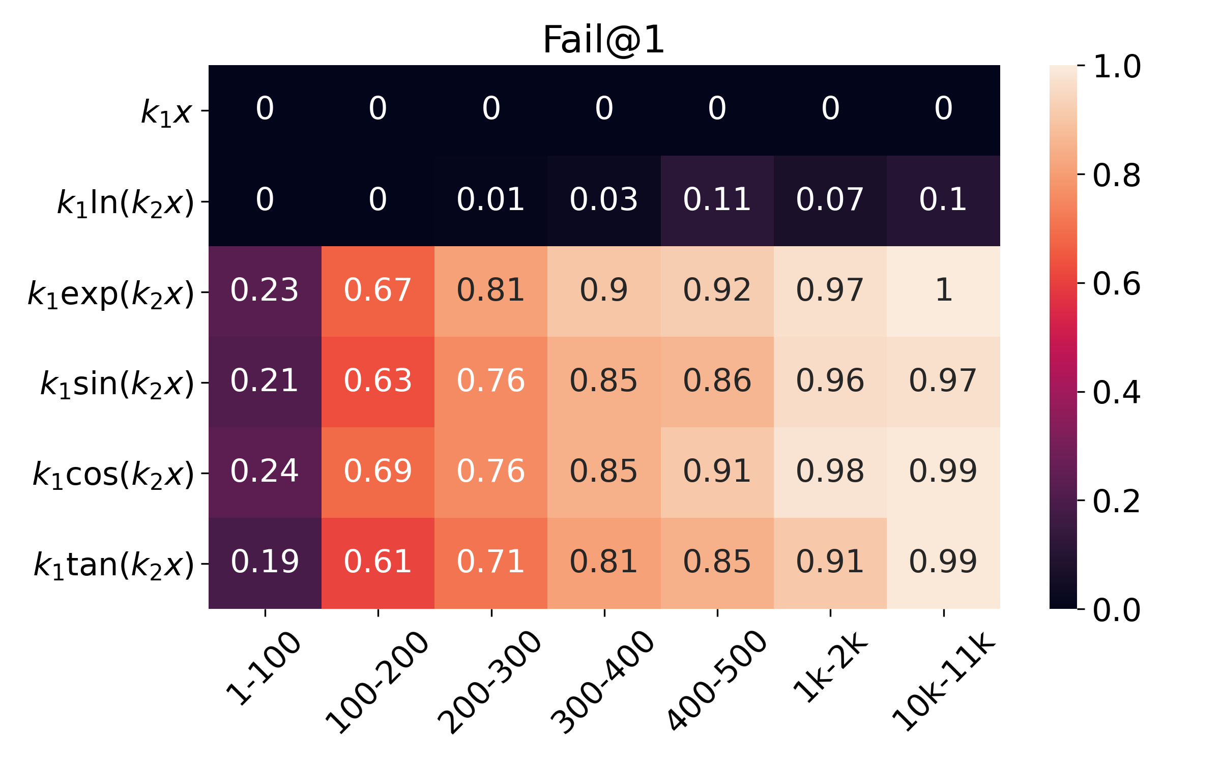
Figure 2: Integer extrapolation. Failure rates for integrating simple primitives with coefficients from the specified range.

Longer problems are more difficult.

First, we use the same data-generating process as for training, but vary its parameters to depart from the training distribution. Specifically, we test extrapolation on number of operator nodes in each equation tree, using Lample and Charton (2019)’s data generation process and varying the max_ops parameter. Table 9 shows performance when max_ops is increased past the model’s training domain (1-15). The neural sequence integrator does show some extrapolation to equation trees with more operator nodes than it was trained on, but its failure rate increases substantially as the number of nodes increases.

Larger failures on larger digits.

Next, we study performance as integer values increase, quickly going out-of-domain. Considering a sample of 200,000 sequences from the training distribution, 99.4% of the positive integers were between 1 and 100. Other ranges were non-empty but sparsely represented; for instance, 0.2% of the integers were between 100 and 200, and 0.096% between 1,000 and 2,000. Figure 2 shows performance on primitive functions with coefficients from the specified range. As in the robustness experiments, the $x$ and $\ln$ primitives perform well, showing that there is some ability to use large numbers. However, performance severely degrades for the $\texttt{exp},\texttt{sin},\texttt{cos},\texttt{tan}$ primitives as the coefficient magnitudes increase, reaching near 100% failure rates on large coefficients.

Problem	Exploit
$169\sin(4x)/x$	Uses $\mathrm{Si}(\cdot)$.
$-2\sin(42/x)$	Uses $\mathrm{Ci}(\cdot)$.
$-2\sin(185x^{2})\cos(2x)$	Uses Fresnel $\mathrm{S},\mathrm{C}$ integrals.
${357^{x^{2}}}^{x}+2\sin(2x)$	Uses incomplete gamma $\Gamma(a,x)$.
$1/(x^{48}(3x+2)^{49})$	Decoding does not terminate.

Table 10: Exploits discovered by SAGGA whose integrals use out-of-domain functions. See Appendix Table 18 for model predictions.

Cluster 1	Cluster 2	Cluster 3	Cluster 4
$119^{x}$	${-240}^{x}+2\cos{2x}$	${-100x}^{x}$	${158x}^{x^{2}}+611$
$132^{x}$	${-398}^{x}+2\cos{2x}$	${-149x}^{x}$	${256x}^{x^{2}}+191$
$136^{x}$	${-692}^{x}+2\sin{2x}$	${-151x}^{x}$	${332x}^{x^{2}}+559$

Table 11: SAGGA discovers many failures that involve $x$ in an exponent. See Appendix Table 17 for model predictions.

Discovering unsupported functionality.

Next, we run SAGGA in an unconstrained setting with all mutation types, favoring short problems using the fitness, $F(f_{\theta},\mathbf{x})=m(\mathbf{x},f_{\theta}(\mathbf{x}))\cdot\frac{1}{|\mathbf{x}|},$ which is positive when the model returns an incorrect integral for $\mathbf{x}$, and higher for shorter problems.

SAGGA discovers exploits based on the neural sequence integrator’s limited training distribution, such as problems whose integral is expressed using the Gamma function $\Gamma(\cdot)$, or the cosine integral $\mathrm{Ci}$, which are not included in its training data (Table 10). These examples are a reminder that the sequence-to-sequence paradigm determines which functions are ‘built in’ by inclusion in training data; omitted behavior is left unspecified, leaving it susceptible to exploits.

Finally, the last problem in Table 10 caused the neural sequence integrator to enter a non-terminating loop during decoding (Appendix Table 18), a known idiosyncrasy of autoregressive models with beam search (Welleck et al. 2020).

SAGGA also finds many clusters that indicate the neural sequence integrator struggles when $x$ appears in an exponent. The discovered problems in Table 11 are a microcosm of our previous findings: For the first cluster, we manually found a nearby problem, $30^{x}$, that the model gets correct; this cluster is a robustness failure. The second cluster shows how such failures cascade further as the function is composed. The final two clusters involve $x^{x}$ or $x^{x^{2}}$, which do not have analytical integrals; these clusters are exploits.

Finding problems with target properties.

Finally, we generate failures of a target length, by running SAGGA to target length 10, 20, and 40 problems. As seen in Figure 3, SAGGA converges to find problems of the target length. Based on our extrapolation experiments, we expect SAGGA to fail more often on longer equations. The right-hand plot in Figure 3 shows that it is also easier to find failures for longer equations, in that the archive grows more quickly for longer target lengths. While we visually inspect short equations for interpretability, the growth rate is a reminder that the space of failures is vast for longer equations.

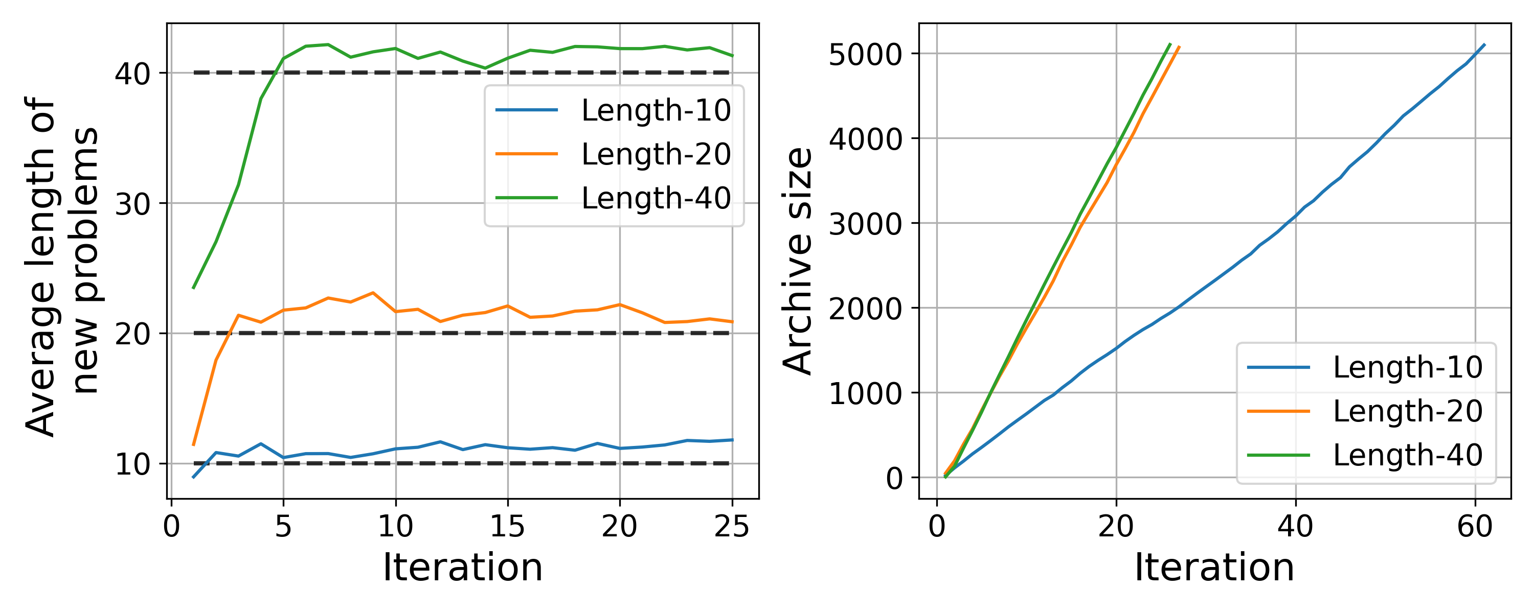
Figure 3: Left: Average length of discovered problems in each iteration, using fitness functions that promote the given length. SAGGA discovers problems of each target length. Right: SAGGA discovers longer problems at a higher rate.

6 Is it a search problem? Distinguishing between model and search errors

	$p$@1	$p$@500	$p$@{1-500}
Failures@500	0.93912	3.9$\times 10^{-6}$	0.99435
Success@500	0.91647	3.5$\times 10^{-6}$	0.99316

Table 12: Probability assigned to the top candidate ($p$@1), the 500’th candidate ($p$@500), and the mass covered by the top 500 candidates ($p$@{1-500}), in failures and successful cases (exp-robustness problems, width-500 beam search). Sequences outside of the top 500 are very improbable compared to the most probable candidate. In both cases, the top 500 candidates cover most of the probability mass.

k	Unresolved@k
1	91.6%
10	65.2%

Table 13: Percentage of failures on the FWD validation set in which the ground truth $\mathbf{y}_{*}$ is scored lower than the top beam candidate (Unresolved@1) or the bottom beam candidate (Unresolved@10), meaning that perfect search would leave the failures at level $k$ unresolved.

Both the experiments of Lample and Charton (2019) and our own generate candidate solutions from a sequence-to-sequence model using beam search. This raises the possibility that failures are due to search rather than the model: what if the highest scoring sequences are correct, but not found?

Specifically, we want to distinguish between search errors, which occur when $p_{\theta}(\mathbf{y}_{*}|\mathbf{x})\gg p(\mathbf{y}|\mathbf{x})$ but the search algorithm (e.g. beam search) does not return $\mathbf{y}_{*}$, and model errors, meaning $p_{\theta}(\mathbf{y}|\mathbf{x})\gg p(\mathbf{y}_{*}|\mathbf{x})$. Here $\mathbf{y}_{*}$ is any correct solution to problem $\mathbf{x}$.

6.1 The model is deficient: model errors.

We study simple-robustness and in-distribution problems, and find evidence of model deficiencies that would remain unresolved with perfect search.

Robustness.

First, we study the simple-primitive robustness problems (e.g. $k_{1}\exp(k_{2}x)$, see Table 2), as these short problems resulted in a small number of timeouts, allowing us to scale up search and verification. We increase the beam size to 500 candidates, and study the model’s probabilities on the 500 returned candidates and correct solutions. We refer to the candidates ranked by decreasing probability as $\mathbf{y}_{\text{beam}}^{(1)},\ldots,\mathbf{y}_{\text{beam}}^{(500)}$ (i.e. $\mathbf{y}_{\text{beam}}^{(1)}$ has the highest probability).

When a correct solution is within the 500 returned candidates, the correct solution often has much lower probability than the top candidate, $p_{\theta}(\mathbf{y}_{\text{beam}}^{(1)}|\mathbf{x})\gg p(\mathbf{y}_{*}|\mathbf{x})$. Specifically, correct solutions often appear at the bottom of the candidates (Figure 4, orange), yet on average the bottom candidate $\mathbf{y}_{\text{beam}}^{(500)}$ has probability $\approx 0.0000035$, while the top candidate $\mathbf{y}_{\text{beam}}^{(1)}$ has probability $\approx 0.92$ (Table 12). These are model deficiencies: the model is confidently incorrect, assigning very high probability to an incorrect solution at the top, and very low probability to correct solutions.

When a correct solution is not within the top 500 candidates, the model is again confidently incorrect, with the top candidate $\mathbf{y}_{\text{beam}}^{(1)}$ receiving $\approx 0.94$ probability. Improving the search algorithm – e.g. by further increasing the search budget or using an alternative to beam search – would inevitably return a low probability solution, as the 500 candidates already cover more than $99.4\%$ of the probability mass (Table 12). The findings again point to model errors.

In-distribution.

Next, we study in-distribution problems from the FWD validation set of Lample and Charton (2019). On failure cases, we test if the ground-truth $\mathbf{y}_{*}$ is scored above the top $k$ beam candidates, meaning that failure@$k$ might be resolved with perfect search–$\mathbf{y}_{*}$ was scored more highly but was simply not found. As seen in Table 13, the majority of failures – 91.6% for failure@1 and 65.2% for failure@10 – would remain unresolved with perfect search, again pointing to model deficiencies.

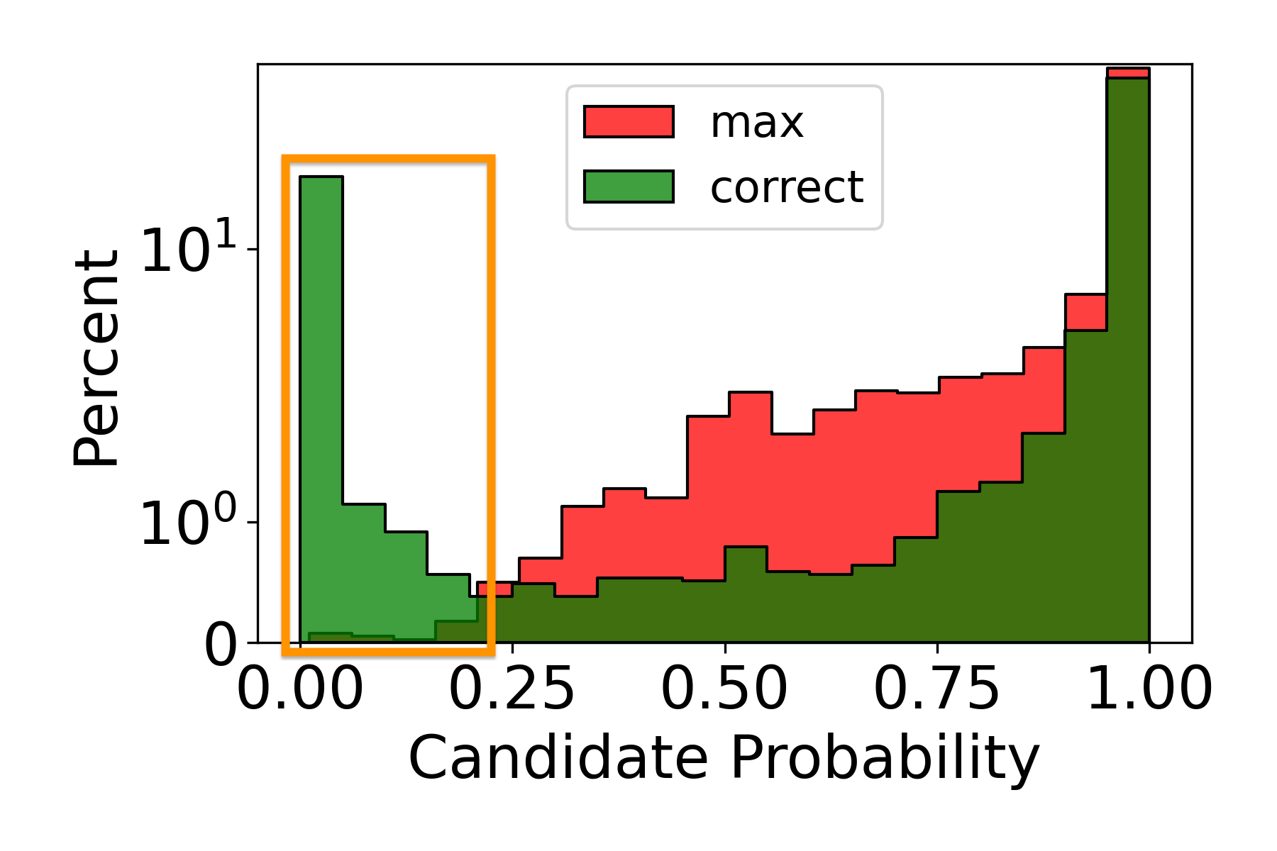
Figure 4: Probabilities assigned to the top-ranked beam candidate (max) versus correct candidates (correct) with a large search & verification budget (500 candidates). The model often assigns very low probability to correct candidates that are found by increasing the search budget; search covers up underlying model deficiencies. (exp-robustness)

6.2 Covering up deficiencies with search.

Our preceding experiments showed that the top of the model’s ranked solution list is often made up of incorrect solutions, while correct solutions deeper into the solution list are assigned very low probabilities. A natural question is whether we can simply ‘cover up’ the deficient model by enumerating and verifying even more candidates, while ignoring the model’s probabilities.

On simple robustness problems (e.g. $k_{1}\exp(k_{2}x)$), we find that large search budgets can alleviate failures, i.e. Fail@$k$ decreases as $k$ increases, for instance moving from roughly 30% failure@1 to 3% failure@500 on exp robustness (Figure 6). On more complex problems, verifying more candidates reduces the failure rate, yet our experiments do not indicate that failures approach zero for practical search budgets. For instance, in our compositionality exp experiments (Table 8), verifying 50 instead of 1 candidate reduces failures, but not below 90%. Larger search budgets quickly become impractical to verify: for compositionality exp, the verification time increases substantially, from around 5 minutes for 1 candidate to over 2 hours for 50, with worst-case verification time of 41.6 hours (Table 14). Looking ahead, developing methods that decrease search and verification cost can help to further cover up a subset of model errors, yet improving the underlying model remains a core issue.

Candidates	Verify (hrs)	Worst-case (hrs)
1	0.088	0.833
10	0.463	8.333
50	2.250	41.667

Table 14: Runtime needed to verify the 3,000-problem exponent compositionality cases (exp, Table 8) with Sympy, using $k$ candidates for $k\in\{1,10,50\}$.

7 Related Work

In this work, we study systematic generalization in sequence models applied to symbolic integration, in terms of robustness, compositionality, and extrapolation, and develop a genetic algorithm for building adversarial problem sets.

Symbolic mathematics and sequence models.

Several works study extrapolation to longer sequences and larger digits in synthetic arithmetic and basic mathematics tasks (Zaremba and Sutskever 2014; Trask et al. 2018; Saxton et al. 2019; Nogueira, Jiang, and Li 2021). Sequence models have also been applied to polynomial rewriting (Piotrowski et al. 2019; Agarwal, Aditya, and Goyal 2021), and differential system stability (Charton, Hayat, and Lample 2021). For symbolic integration, Davis (2019) argue that the neural sequence integrator’s test performance should be qualified, though without an empirical demonstration. These critiques motivate our focus on the neural sequence integrator (Lample and Charton 2019), whose performance we characterize and empirically study in terms of systematic generalization.

Systematic generalization.

Several works identify difficulties with modern methods on synthetic tasks (e.g. Lake and Baroni (2018); Bahdanau et al. (2019); Hupkes et al. (2020); Kim and Linzen (2020)) and machine translation (Raunak et al. 2019), with a focus on compositionality and extrapolation. Some methods address systematicity with inductive biases in model structure (Andreas et al. 2016; Bahdanau et al. 2019), and others through the data (Hill et al. 2020; Andreas 2020) or learning procedure (Lake 2019; Vani et al. 2021). We focus on systematic generalization deficiencies in a state-of-the-art model in a new setting – symbolic integration – with additional aspects of generalization.

Robustness and adversaries in sequence models.

Several works study robustness in NLP, including classification (Tu et al. 2020), word substitutions (Jia et al. 2019), domain shift in QA (Kamath, Jia, and Liang 2020) or topic distributions (Oren et al. 2019). Several methods find adversarial examples in NLP (Morris et al. 2020). Alzantot et al. (2018) use genetic algorithms in a classification setting, while we consider generation. Michel et al. (2019) constrain input sequences to be similar and use a gradient-based attack to swap tokens. We face a non-differentiable cost and generate large collections of failures with a wide class of mutations.

8 Conclusion

We study generalization in symbolic mathematics using the predominant modeling paradigm: a large-scale transformer trained with maximum likelihood. We find deficiencies that are not captured by test accuracy, including brittleness to small perturbations, difficulty composing known solutions, and gaps in the training distribution. We offer speculations based on our results. Due to the large space of equations, practical empirical distributions do not provide a dense sampling of individual problem types (e.g. $k_{1}\cos(k_{2}x)$), and each empirical sample contains shared biases from the underlying data generator (e.g. integer values, lengths). Thus, sparse test sets do not adequately measure systematic generalization. From a learning perspective, generic networks trained with SGD do not necessarily favor the simplest hypothesis to explain the data; thus a sparse training set yields an underconstrained hypothesis space, with hypotheses that do not strongly generalize (e.g. Table 5), causing behavior that breaks simple rules (e.g. adhering to a template or following the sum rule). We suspect that inductive biases– e.g. encoded through the training distribution, architectural components, or learning algorithm– are needed to narrow the hypotheses to those that strongly generalize.

Appendix A Additional Results

A.1 Large Search Budgets

We study the simple-primitive robustness problems (from Table 2, top), as these problems resulted in a small number of Sympy timeouts, allowing for scaling of verification. We increase the beam-width to 500 candidates, and show Fail@k for $k\in\{1,10,50,200,500\}$ in Figure 6. The top of the solution list remains brittle with the larger beam size: that is, with beam size 500 the top-ranked solutions are still frequently incorrect, supporting the findings in Table 13. However, the correct solution often exists deeper into the ranked list, i.e. Fail@k decreases as $k$ increases, ranging from 0.1 Fail@500 for cos to 3.7 Fail@500 for tan. As an illustration, Figure 6 shows the ranking of the correct solution for exp-robustness problems that had a solution in the top-500 beam candidates.

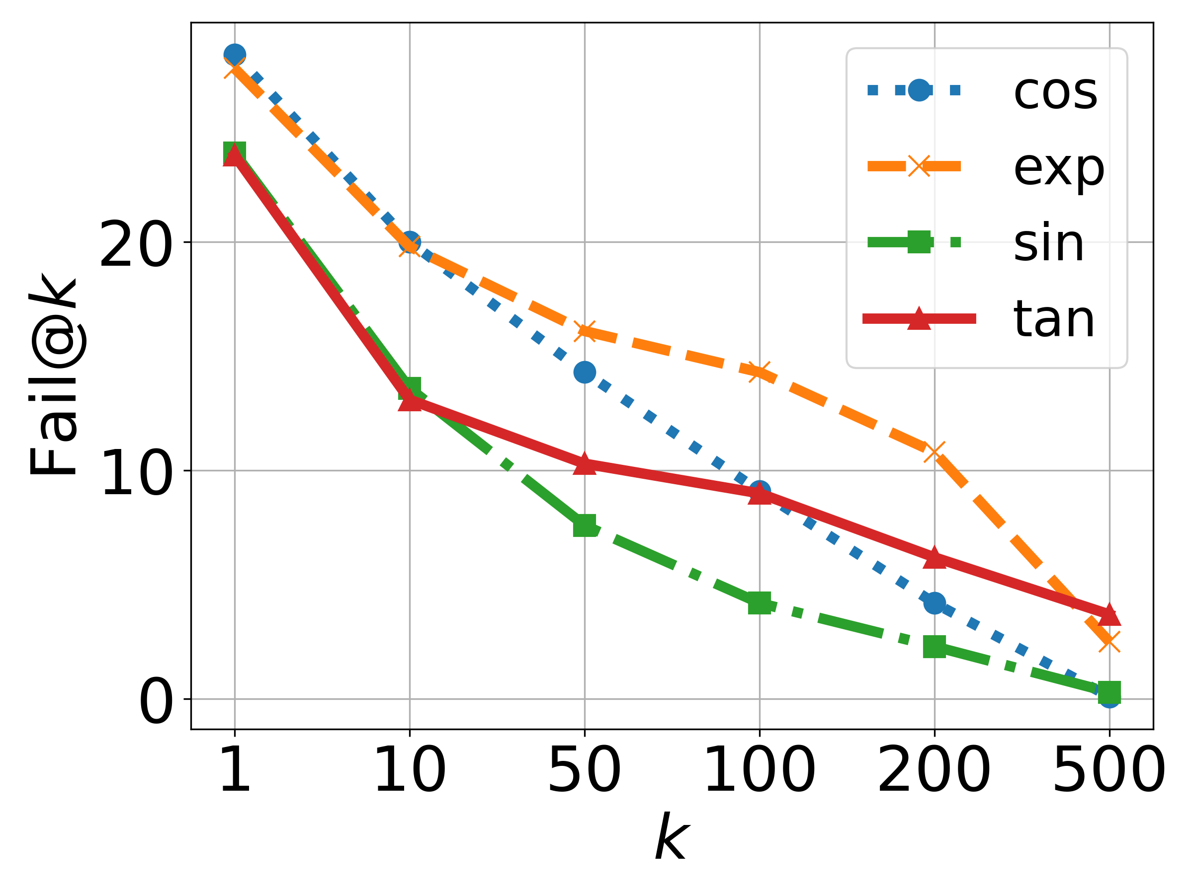
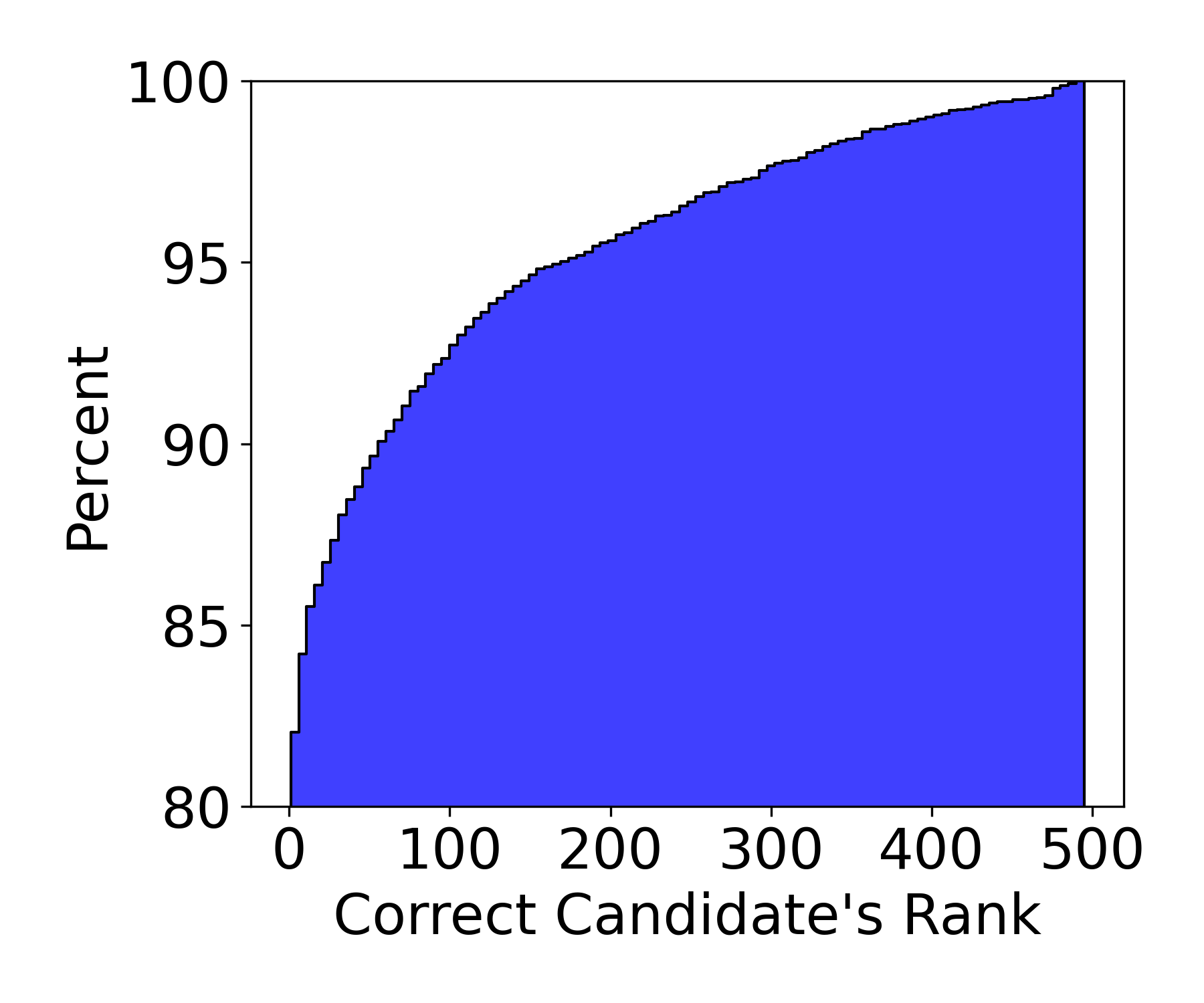
Figure 5: Fail@k with a large search-and-verify budget (500 candidates, beam search) on simple-primitive robustness problems. The model is ‘brittle’ in that the top of its ranked solution list is often made up of incorrect solutions; e.g. the top-ranked solution is incorrect around 25% of the time. However, the correct solution often exists within the model’s top 500 predictions on these problems.

Figure 6: Correct candidate’s ranking out of 500 candidates (beam search) on exp-primitive robustness problems.

A.2 Alternate Decoding Strategies

So far, we have used beam search, a deterministic search that approximately searches for the highest scoring output sequence. An alternative approach is decoding a set of sequences $\{\hat{}\mathbf{y}_{1},\ldots,\hat{}\mathbf{y}_{k}\}$ by sampling recursively from model-dependent per-token distributions, $y_{t}^{(i)}\sim q(y_{t}|y_{<t},\mathbf{x},p_{\theta})$, where each $\hat{}\mathbf{y}_{i}=(y_{1}^{(i)},\ldots,y_{T_{i}}^{(i)})$. We use the common approach of temperature sampling.

Figure 7 shows Fail@k rates for sampling 500 candidates at temperatures $\{0.6,0.8,1.0\}$, and beam search with 500 candidates, for exp-robustness problems (other simple-primitives gave similar results). Beam search outperforms sampling, which we attribute to better exploration with beam search: namely, beam search guarantees unique candidates, while sampling returns many duplicates in this setting (here, only 14 unique sequences out of 500 samples).

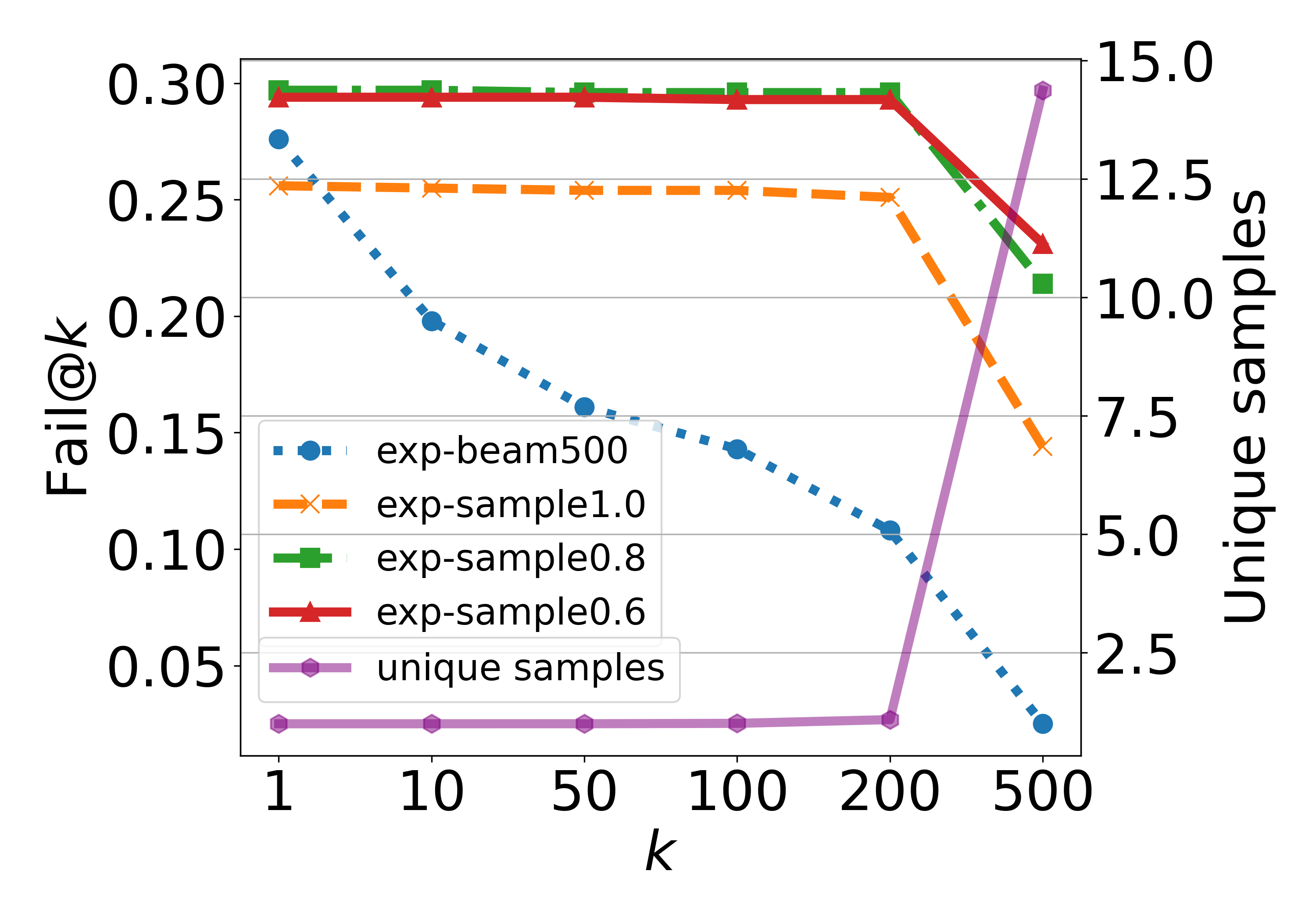
Figure 7: Comparing Fail@k using sampling vs. beam search on exp-robustness. Beam search outperforms sampling, which we attribute to better exploration with beam search: namely, beam search returns unique candidates, while sampling returns many duplicates in this setting.

A.3 SAGGA – Quantitative Summary

Table 15 provides a quantitative summary of the archives discovered with SAGGA. Figure 8 shows the rate at which SAGGA fills its archive with failure cases under different mutation strategies and fitness functions.

	Iters	Len	Nodes	Depth	1-term	2-term	3-term
General	3	15.4	7.3	3.6	64.8	24.7	10.5
General-Trig	3	21.8	11.1	4.9	55.7	36.6	7.7
Robust-Trig	4	16.4	7.7	4.5	69.9	30.1	0.0
Robust-Poly	4	23.6	12.6	3.9	17.0	24.1	43.7
Distance	3	30.0	15.0	5.4	32.6	34.2	20.2
Length-10	61	11.1	5.3	3.1	91.3	8.6	0.1
Length-20	27	21.4	10.0	4.2	58.0	35.5	6.4
Length-40	26	40.6	16.7	5.5	13.5	49.3	34.3

Table 15: Summary of the archives discovered with SAGGA for the target failure type shown on the left. Iters gives the number of SAGGA iterations needed to reach 1,000 failures, and 5,000 failures for the Length-X settings. We use the number of + operations plus 1 as a rough proxy for the number of ‘terms’ in a problem; e.g. $x^{2}+2$ has 2 terms.

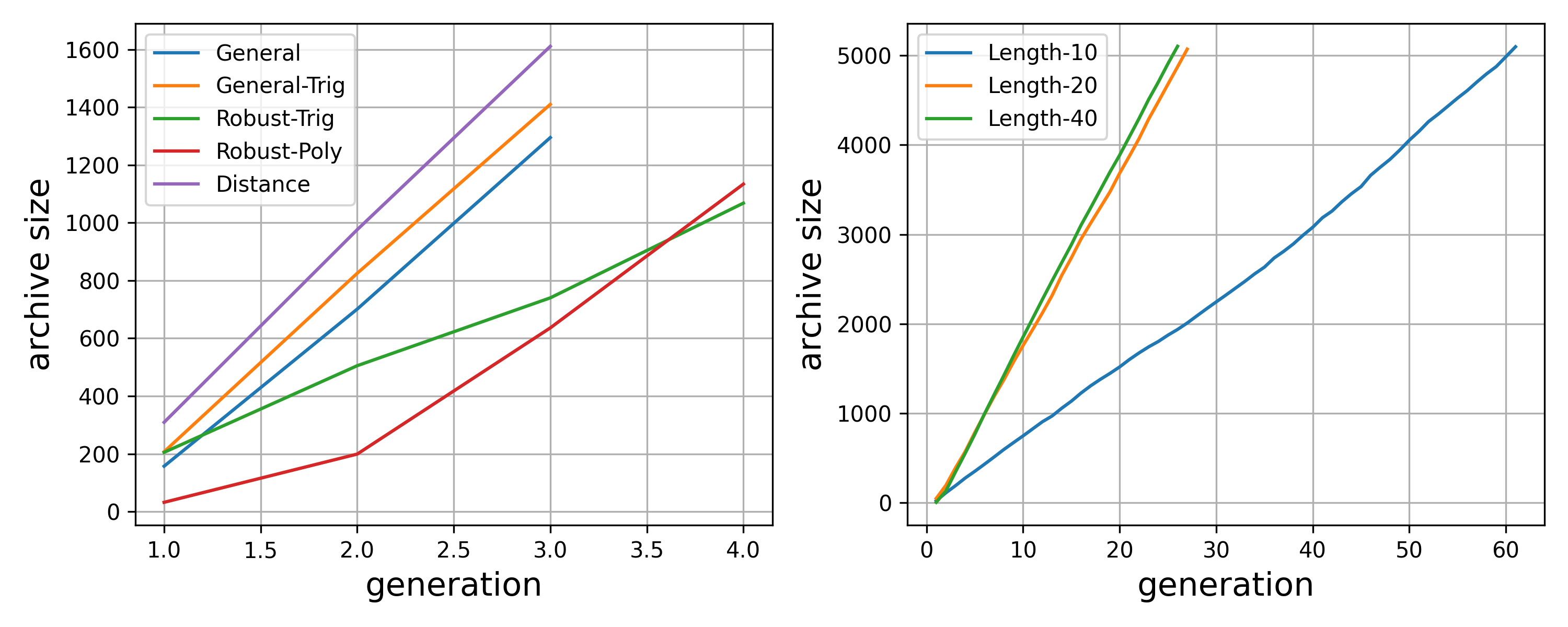
Figure 8: Cumulative failures found per iteration of SAGGA, for various mutation and fitness settings.

Appendix B Additional Experiment Details

B.1 Experimental Setup

We use the implementation and pre-trained model from Lample and Charton (2019) for all of our experiments, specifically the FWD+BWD+IBP model which obtained top-10 accuracies of 95.6%, 99.5%, and 99.6% on their publicly available test sets. Our evaluation is based on their code provided in beam_integration.ipynb. We use their utilities for inputs and outputs, and by default use beam search with beam size 10. When computing Fail@50 we use beam size 50. Following Lample and Charton (2019), we use Sympy to check whether the derivative of a prediction is equal to the original problem, simplify(derivative - f) == 0. We generously count the prediction as correct if a timeout occurs. Since Sympy’s simplify function is imperfect, there is a possibility of false negatives, which is an inherent limitation of verifying whether a solution is correct. However, an answer that is not feasibly verifiable in a search-and-verify setting is incorrect for practical purposes. In preliminary experiments, we found that additionally simplifying the derivative and the function before subtracting tended to reduce timeouts, and found that Sympy’s ability to simplify hyperbolic functions (e.g. $\sinh,\cosh$) was limited, so we discard problems with hyperbolic functions from our analysis. Future work could verify with additional libraries, and we release all predictions for inspection.

B.2 Robustness

Test accuracy does not imply robustness.

For $X_{\mathcal{N}_{1}}$ we sample 100 successful validation problems $f$ and $10$ values of $k$, while for $X_{\mathcal{N}_{2}}$ we sample 1000 successful validation problems.

B.3 Compositionality

Validation problems.

Fail@50 valid had abnormally many timeouts compared to the other experiments; for this setting only we do not consider a timeout as correct.

B.4 Extrapolation

More details of integer distribution.

As a rough picture of integer values in the training distribution, we sample 100,000 sequences from each of the FWD and BWD train sets, convert them to Sympy, and count Sympy equation tree nodes of type Integer. We find that 99.4% of the positive integers were in the range [1, 100), and that other magnitude buckets were non-empty but sparsely represented – e.g. [100, 200) had 0.2%, and [1000, 2000) had 0.096% ,and [10000, 20000) had 0.005% of the positive integers in the problem sample.

B.5 Runtime vs. Candidates

We generously stop early if a successful candidate is found, and use a 1-second timeout for Sympy; thus the results are a lower-bound on the runtime. In the worst case, for $N$ problems, without early stopping and with a $t$-second timeout, verification takes $O(ktN)$ seconds, e.g. 41.6 hours to verify 50 candidates on 3,000 problems with a 1 second timeout.

Appendix C SAGGA

Default fitness.

Unless otherwise noted, we use a fitness that favors short (and hence interpretable) problems,

$$F(f_{\theta},\mathbf{x}) =m(\mathbf{x},f_{\theta}(\mathbf{x};1))\cdot\frac{1}{|\mathbf{x}|},$$ (6)

which is positive when the model returns an incorrect integral of problem $\mathbf{x}$, and higher for shorter problems.

Mutations.

A mutation transforms a problem’s equation tree; i.e. $h(T_{\mathbf{x}})\rightarrow T^{\prime}$ where $T_{\mathbf{x}}$ is the equation tree of problem $\mathbf{x}$. SAGGA supports mutations for internal tree nodes and leaf nodes.

The internal node mutations replace a node $v_{i}$ with:

• Constant: an integer $k\sim\mathcal{U}(v_{\text{min}},v_{\text{max}})$.

• Symbol: $x$.

• Operation: $v_{i}^{\prime}\sim\{+,*,**\}$

• Add-arg: $v_{i}^{\prime}(w_{1:j},w_{j+1})$, where $w_{1:j}$ are the previous arguments to $v_{i}$ and $w_{j+1}$ is a random simple operation (see below). For instance, $\texttt{sum}(1,2)\rightarrow\texttt{sum}(1,2,3x^{2})$. If $v_{i}$ is a one-argument function, this mutation adds a new argument via a sum, e.g. $\texttt{exp}(1)\rightarrow\texttt{exp}(1+3x^{2})$.

The leaf node mutations replace a node $v_{i}$ with:

• Constant: an integer $k\sim\mathcal{U}(v_{\text{min}},v_{\text{max}})$.

• Symbol: $kx$ where $k\sim\mathcal{U}(v_{\text{min}},v_{\text{max}})$.

• Simple-op: random simple operation (see below).

Each random simple operation is of the form $k_{1}\circ x^{k}_{2}$, where $k_{1}\sim\mathcal{U}(v_{\text{min}},v_{\text{max}})$, $\circ\sim\{*,**,/\}$, $k_{2}\sim\{1,2\}$. For instance, $3x^{2}$, $5/x$.

Default settings.

Unless otherwise noted, we run SAGGA with the following default settings:

• Beam size: 10

• Evaluation $m(\mathbf{x},\cdot)$: Fail@1

• Seed size: 100

• Generation size: 1000

• Seed selection: k-means, $k=10$

• Fitness threshold $\tau$: 0.01

• Target archive size: 1000

• Integer perturbation range $v_{\text{min}},v_{\text{max}}$: [-1000, 1000]

• Mutations: all

• Seed problems: $\{1,\quad x,\quad x+1,\quad x^{2}+x+1\}$

Each generation (iteration) takes around 4 minutes on a single Quadro RTX 8000 GPU.

C.1 Robustness.

Settings.

• Integer perturbation range $v_{\text{min}},v_{\text{max}}$: [-100, 100]

• Mutations: only Constant mutations.

Seeds.

Polynomial robustness:

$$X_{\texttt{poly}}=\{ 1,2x,2/x,2x+1,2/x+1,$$

$$2x^{2}+2x+1,2x^{2}+2/x+1,$$

$$2x^{3}+2x^{2}+1,$$

$$2x^{42}+2x^{3}+2x^{2}+1\}$$

Trigonometric robustness:

$$X_{\texttt{trig}}=\{ 17\cos(83x),17\cos(83x)+1,$$

$$34\sin(77x),34\sin(77x)+1$$

$$2\cos(2x)+2x,2\cos(2x)+2x+1,$$

$$2\sin(2x)+2x,2\sin(2x)+2x+1$$

$$2\sin(2x)\cos(2x)\}$$

In these experiments, the structure of the seeds remains fixed and the integers are varied. The seed elements with non-trivial integers were selected based on the manual neighborhood experiments. Note that this simply accelerates the experiment, as the algorithm could discover these.

C.2 Out-of-distribution.

General failures. We run SAGGA in two settings. The first is with default settings (see above). The second biases the search towards trigonometric functions, using the seed,

$$X_{\texttt{trig-general}}=\{ 2\cos(2x),2\cos(2x)+1$$

$$2\sin(2x),2\sin(2x)+1$$

$$2\cos(2x)+2x,2\cos(2x)+2x+1,$$

$$2\sin(2x)+2x,2\sin(2x)+2x+1$$

$$2\sin(2x)\cos(2x)\}$$

and set the default fitness to zero unless the problem contains a trigonometric function.

Target lengths. We use the fitness,

$$F(f_{\theta},\mathbf{x}) =m(\mathbf{x},f_{\theta}(\mathbf{x};1))\cdot\frac{1}{|\mathbf{x}-\ell|},$$ (7)

where $\ell$ is the target length.

To more clearly compare growth rates, compared to the other experiments we use a smaller seed size of 50 and smaller generation size of 300, and generate 5,000 failures rather than 1,000, resulting in more iterations per algorithm setting.

x	hyp_simplified	derivative	difference
-103	-103*x	-103	0
-104	-48*x - 625	-48	56
-136	-128*x	-128	8
-33	-31*x - 256	-31	2
2*x**(42)+21	x*(2*x**42 + 903)/43	2*x**42 + 21	0
2*x**(42)+22	2*x*(x**42 + 469)/43	2*x**42 + 938/43	-8/43
2*x**(42)+28	2*x*(x**42 + 614)/43	2*x**42 + 1228/43	24/43
2*x**(42)+68	2*x*(x**42 + 1502)/43	2*x**42 + 3004/43	80/43
-47 + 2/x - 2/x**70	-47*x + 2*log(x) + 2/(69*x**69)	-47 + 2/x - 2/x**70	0
-47 + 2/x - 2/x**71	-47*x + 2*log(x) + 2/(35*x**70)	-47 + 2/x - 4/x**71	-2/x**71
-47 + 2/x - 31/x**71	-47*x + log(x**2) + x**(-60)	-47 + 2/x - 60/x**61	(31 - 60*x**10)/x**71
-71 + 36/x - 2/x**71	-71*x + 36*log(x) + 1/(17*x**70)	-71 + 36/x - 70/(17*x**71)	-36/(17*x**71)
13*cos(18*x)	13*sin(18*x)/18	13*cos(18*x)	0
13*cos(19*x)	sin(19*x)	19*cos(19*x)	6*cos(19*x)
13*cos(83*x)	sin(83*x)/17	83*cos(83*x)/17	-138*cos(83*x)/17
17*cos(47*x)	sin(47*x)	47*cos(47*x)	30*cos(47*x)
13*cos(82*x) - 59	-59*x + 13*sin(82*x)/82	13*cos(82*x) - 59	0
13*cos(83*x) - 59	-59*x + sin(83*x)/13	83*cos(83*x)/13 - 59	-86*cos(83*x)/13
17*cos(37*x) - 49	-49*x + sin(37*x)	37*cos(37*x) - 49	20*cos(37*x)
17*cos(41*x) - 45	-45*x + sin(41*x)	41*cos(41*x) - 45	24*cos(41*x)
10*sin(45*x)*cos(2*x)	-5*cos(43*x)/43 - 5*cos(47*x)/47	5*sin(43*x) + 5*sin(47*x)	0
10*sin(47*x)*cos(2*x)	-255*cos(45*x)/2201 - 215*cos(49*x)/2201	11475*sin(45*x)/2201 + 10535*sin(49*x)/2201	470*sin(45*x)/2201 - 470*si…
10*sin(90*x)*cos(2*x)	-5*cos(43*x)/44 - 5*cos(47*x)/46	215*sin(43*x)/44 + 235*sin(47*x)/46	215*sin(43*x)/44 + 235*sin(47…
19*sin(90*x)*cos(2*x)	cos(2*x)**2*cos(90*x)/2	-2*sin(2*x)*cos(2*x)*cos(90*x) - 45*sin(90*x)*…	-(43*sin(88*x)/2 + 19*sin…
-x**2 + x + log(4)*tan(x)	-x**3/3 + x**2/2 - log(4)*log(cos(x))	-x**2 + x + log(4)*sin(x)/cos(x)	0
-x**2 + x + log(4)*tan(17*x**2)	-x**3/3 + x**2/2 + log(2)*log(cos(17*x**2)…	-x**2 + 2*x*log(2)*sin(17*x**2)/cos(17*x**2) + x	(x - 1)*log(4)*tan(17*x**2)
-x**2 + x + log(4)*tan(2*x**2)	-x**3/3 + x**2/2 + log(2)*log(cos(2*x**2)…	-x**2 + 4*x*log(2)*sin(2*x**2)/cos(2*x**2) + x	(2*x - 1)*log(4)*tan(2*x**2)
-x**2 + x + log(4)*tan(63/x**2)	-x**3/3 + x**2/2 - log(2)*log(cos(63/x**2)…	-x**2 + x + 252*log(2)*sin(63/x**2)/(x**3*cos(…	(126 - x**3)*log(4)*tan(63/…
sqrt(3*x + 3) - 2	-2*x + 2*sqrt(3)*(x + 1)**(3/2)/3	sqrt(3)*sqrt(x + 1) - 2	0
sqrt(-86**(x**2) + 62/x) - 40	-40*x + acosh(86**(-x**2/2)/x)	-40 + (-86**(-x**2/2)*log(86) - 86**(-x**2/2)/…	-sqrt(-86**(x**2) + 62/x) …
sqrt(14 + 62/x) + 4	(49*x**(3/2) + 217*sqrt(x) + sqrt(7*x + 31…	(147*sqrt(x)/2 + (28 + sqrt(749)/(sqrt(x)*sqrt…	(-x*(7*x + 31)**(5/2)*sqrt(2…
sqrt(14 + 62/x) - 2	(49*x**(3/2) + 217*sqrt(x) + (-14*x + 31*…	(147*sqrt(x)/2 + (-14 + sqrt(854)/(2*sqrt(x)*s…	(x*(7*x + 31)**(5/2)*sqrt(6…
tan(exp(2))/(18*x)	log(x)*tan(exp(2))/18	tan(exp(2))/(18*x)	0
tan(26*x + 2 + exp(2))/(18*x**75)	[add, mul, div, INT-, 1, INT+, 1, 5, 1, 2, mul…	–	–
tan(exp(-9504*x**2))/(18*x)	-log(cos(exp(-9504*x**2))**(-2))/18144	44*x*exp(-9504*x**2)*sin(exp(-9504*x**2))/…	44*x*exp(-9504*x**2)*sin(…
tan(exp(-96*x))/(18*x)	-log(cos(exp(-96*x))**(-2))/1728	exp(-96*x)*sin(exp(-96*x))/(9*cos(exp(-96*x)))	(2*x - exp(96*x))*exp(-9…

Table 16: SAGGA robustness. We show the problem $\mathbf{x}$, the simplified prediction from the neural sequence integrator, its derivative, and the derivative’s difference with $\mathbf{x}$. The prediction is incorrect when the difference is not zero. When the model’s prediction does not parse successfully, we show its unparsed infix tokens. We show a nearby problem that the model gets correct in bold (either hand-selected or a validation example); all other problems are failures discovered by SAGGA.

	x	hyp_simplified	derivative	difference
0	30**x	30**x/log(30)	30**x	0
1	119**x	119**(x - 1)	119**(x - 1)*log(119)	119**(x - 1)*(-119 + log(119))
2	132**x	132**x/(1 + log(132))	132**x*log(132)/(1 + log(132))	-132**x/(1 + log(132))
3	136**x	exp(x*log(136))	exp(x*log(136))*log(136)	-136**x + exp(x*log(136))*log(136)
4	-100*x**x	-50*x**2	-100*x	-100*x + 100*x**x
5	-149*x**x	-149*x**2/2	-149*x	-149*x + 149*x**x
6	-151*x**x	-151*x**2/2	-151*x	-151*x + 151*x**x
7	158*x**(x**2) + 611	158*x**2/sqrt(x**2 + 1) + 611*x	-158*x**3/(x**2 + 1)**(3/2) + 316*x/sqrt(x**2 + 1) + 611	-158*x**3/(x**2 + 1)**(3/2) + 316*x/sqrt(x**2 + 1) - 158*x**(x**2)
8	256*x**(x**2) + 191	x*(191*x**2 + 256*x**(x**2) + 191)/(x**2 + 1)	-2*x**2*(191*x**2 + 256*x**(x**2) + 191)/(x**2 + 1)**2 + x*(382*x + 256*x**(x**2)*(2*x*log(x) + x))/(x**2 + 1) + (191*x**2 + 256*x**(x**2) + 191)/(x**2 + 1)	512*x**(x**2 + 2)*(x**2*log(x) + log(x) - 1)/(x**4 + 2*x**2 + 1)
9	332*x**(x**2) + 559	x*(559*x**2 + 332*x + 559)/(x**2 + 1)	-2*x**2*(559*x**2 + 332*x + 559)/(x**2 + 1)**2 + x*(1118*x + 332)/(x**2 + 1) + (559*x**2 + 332*x + 559)/(x**2 + 1)	332*(2*x - x**(x**2) - 2*x**(x**2 + 2) - x**(x**2 + 4))/(x**4 + 2*x**2 + 1)
10	-240**x + 2*cos(2*x)	-exp(x*log(240)) + sin(2*x)	-exp(x*log(240))*log(240) + 2*cos(2*x)	240**x - exp(x*log(240))*log(240)
11	-398**x + 2*cos(2*x)	-exp(x*log(398)) + sin(2*x)	-exp(x*log(398))*log(398) + 2*cos(2*x)	398**x - exp(x*log(398))*log(398)
12	-692**x + 2*sin(2*x)	-exp(x*log(692)) - cos(2*x)	-exp(x*log(692))*log(692) + 2*sin(2*x)	692**x - exp(x*log(692))*log(692)

Table 17: SAGGA OOD – $g(x)^{x}$. We show the problem $\mathbf{x}$ discovered by SAGGA, the simplified prediction from the neural sequence integrator, its derivative, and the derivative’s difference with $\mathbf{x}$. The prediction is incorrect when the difference is not zero. For the first cluster, we manually found a nearby problem that the model gets correct in bold; thus this cluster can be seen as a robustness failure. The second two clusters involve $x^{x}$ or $x^{x^{2}}$ which to our knowledge do not have analytical integrals (e.g. see https://www.wolframalpha.com/input/?i=integral+of+x**x); these clusters can be seen as exploits.

	x	hyp_raw	Correct Integral (Wolfram Alpha)
0	169*sin(4*x)/x	169*log(x**2)/8 - 169*cos(4*x)/4	$169\ \mathrm{Si}(4x)$
1	-2*sin(42/x)	cos(42/x)/21	$-2(-42\mathrm{Ci}(42/x)+x\sin(42/x))$
2	-2*sin(185*x**2)*cos(2*x)	4*sin(2*x)*sin(185*x**2)/3421 + 370*cos(2*x)*cos(185*x**2)/3421	-(Sqrt[Pi/370] (Cos[1/185] FresnelS[Sqrt[2/(185 Pi)] (-1 + 185 x)] + Cos[1/185] FresnelS[Sqrt[2/(185 Pi)] (1 + 185 x)] - (FresnelC[Sqrt[2/(185 Pi)] (-1 + 185 x)] + FresnelC[Sqrt[2/(185 Pi)] (1 + 185 x)]) Sin[1/185]))
3	357**(x**(2**x)) + 2*sin(2*x)	exp(x*log(2)) - cos(2*x)	No result
4	1/(x**48*(3*x+2)**49)	add, mul, div, INT-, 1, 0, 9, 0, 9, 1, 9, 9, 9, 9, 9, 9, 9, 9, 9, 9, 9, 9, 9, 5, INT+, 1, 0, 2, 4, ln, x, add, mul, div, INT+, 1, 0, 9, 0, 9, 1, 9, 9, 9, 9, 9, 9, 9, 9, 9, 9, 9, 9, 9, 9, 9, 9, 9, 9, 9, INT+, 1, 0, 2, 4, ln, add, div, INT+, 2, INT+, 3, x, mul, INT-, 1, mul, pow, add, mul, INT+, 1, 0, 0, 9, 6, 2, 9, 4, 4, 0, 0, 0, 0, 0, 0, 0, 0, 0, 0, 0, 0, 0, 0, 0, 0, 0, 0, 0, 0, 0, 0, 0, 0, 0, 0, 0, 0, 0, 0, 0, 0, 0, 0, 0, 0, 0, 0, 0, 0, 0, 0, 0, 0, 0, 0, 0, 0, 0, 0, 0, 0, 0, 0, 0, 0, 0, 0, 0, 0, 0, 0, 0, 0, 0, 0, 0, 0, 0, 0, 0, 0, 0, 0, 0, 0, 0, 0, 0, 0, 0, 0, 0, 0, 0, 0, 0, 0, 0, 0, 0, 0, 0, 0, 0, 0, 0, 0, 0, 0, 0, 0, 0, 0, 0, 0, 0, 0	See https://www.wolframalpha.com/input/? i=integral+of+1%2F%28x**48*%283*x%2B2%29**49%29

Table 18: SAGGA OOD – exploits. We show the problem $\mathbf{x}$, and the neural sequence integrator’s prediction as either raw prefix tokens or (when possible) in its infix form. All problems are failures discovered by SAGGA.

References

- Agarwal, Aditya, and Goyal (2021) Agarwal, V.; Aditya, S.; and Goyal, N. 2021. Analyzing the Nuances of Transformers’ Polynomial Simplification Abilities. arXiv:2104.14095.
- Agrawal, Batra, and Parikh (2016) Agrawal, A.; Batra, D.; and Parikh, D. 2016. Analyzing the Behavior of Visual Question Answering Models. In Proceedings of the 2016 Conference on Empirical Methods in Natural Language Processing, 1955–1960. Austin, Texas: Association for Computational Linguistics.
- Alzantot et al. (2018) Alzantot, M.; Sharma, Y.; Elgohary, A.; Ho, B.-J.; Srivastava, M.; and Chang, K.-W. 2018. Generating Natural Language Adversarial Examples. In Proceedings of the 2018 Conference on Empirical Methods in Natural Language Processing, 2890–2896. Brussels, Belgium: Association for Computational Linguistics.
- Andreas (2020) Andreas, J. 2020. Good-Enough Compositional Data Augmentation. In Proceedings of the 58th Annual Meeting of the Association for Computational Linguistics, 7556–7566. Online: Association for Computational Linguistics.
- Andreas et al. (2016) Andreas, J.; Rohrbach, M.; Darrell, T.; and Klein, D. 2016. Neural module networks. In Proceedings of the IEEE Computer Society Conference on Computer Vision and Pattern Recognition. ISBN 9781467388504.
- Bahdanau et al. (2019) Bahdanau, D.; Murty, S.; Noukhovitch, M.; Nguyen, T. H.; De Vries, H.; and Courville, A. 2019. Systematic generalization: What is required and can it be learned? In 7th International Conference on Learning Representations, ICLR 2019.
- Beltagy, Lo, and Cohan (2019) Beltagy, I.; Lo, K.; and Cohan, A. 2019. SciBERT: A Pretrained Language Model for Scientific Text. In Proceedings of the 2019 Conference on Empirical Methods in Natural Language Processing and the 9th International Joint Conference on Natural Language Processing (EMNLP-IJCNLP), 3615–3620. Hong Kong, China: Association for Computational Linguistics.
- Charton, Hayat, and Lample (2021) Charton, F.; Hayat, A.; and Lample, G. 2021. Learning advanced mathematical computations from examples. arXiv:2006.06462.
- Davis (2019) Davis, E. 2019. The Use of Deep Learning for Symbolic Integration: A Review of (Lample and Charton, 2019). arXiv:1912.05752.
- Gardner et al. (2020) Gardner, M.; Artzi, Y.; Basmov, V.; Berant, J.; Bogin, B.; Chen, S.; Dasigi, P.; Dua, D.; Elazar, Y.; Gottumukkala, A.; Gupta, N.; Hajishirzi, H.; Ilharco, G.; Khashabi, D.; Lin, K.; Liu, J.; Liu, N. F.; Mulcaire, P.; Ning, Q.; Singh, S.; Smith, N. A.; Subramanian, S.; Tsarfaty, R.; Wallace, E.; Zhang, A.; and Zhou, B. 2020. Evaluating Models’ Local Decision Boundaries via Contrast Sets. In Findings of the Association for Computational Linguistics: EMNLP 2020, 1307–1323. Online: Association for Computational Linguistics.
- Henighan et al. (2020) Henighan, T.; Kaplan, J.; Katz, M.; Chen, M.; Hesse, C.; Jackson, J.; Jun, H.; Brown, T. B.; Dhariwal, P.; Gray, S.; Hallacy, C.; Mann, B.; Radford, A.; Ramesh, A.; Ryder, N.; Ziegler, D. M.; Schulman, J.; Amodei, D.; and McCandlish, S. 2020. Scaling Laws for Autoregressive Generative Modeling. ArXiv, abs/2010.14701.
- Hill et al. (2020) Hill, F.; Lampinen, A.; Schneider, R.; Clark, S.; Botvinick, M.; McClelland, J. L.; and Santoro, A. 2020. Environmental drivers of systematicity and generalization in a situated agent. In International Conference on Learning Representations.
- Holtzman et al. (2020) Holtzman, A.; Buys, J.; Du, L.; Forbes, M.; and Choi, Y. 2020. The Curious Case of Neural Text Degeneration. In International Conference on Learning Representations.
- Hupkes et al. (2020) Hupkes, D.; Dankers, V.; Mul, M.; and Bruni, E. 2020. Compositionality Decomposed: How do Neural Networks Generalise? Journal of Artificial Intelligence Research.
- Jia et al. (2019) Jia, R.; Raghunathan, A.; Göksel, K.; and Liang, P. 2019. Certified Robustness to Adversarial Word Substitutions. In Proceedings of the 2019 Conference on Empirical Methods in Natural Language Processing and the 9th International Joint Conference on Natural Language Processing (EMNLP-IJCNLP), 4129–4142. Hong Kong, China: Association for Computational Linguistics.
- Kamath, Jia, and Liang (2020) Kamath, A.; Jia, R.; and Liang, P. 2020. Selective Question Answering under Domain Shift. In Proceedings of the 58th Annual Meeting of the Association for Computational Linguistics, 5684–5696. Online: Association for Computational Linguistics.
- Kim and Linzen (2020) Kim, N.; and Linzen, T. 2020. COGS: A Compositional Generalization Challenge Based on Semantic Interpretation. In Proceedings of the 2020 Conference on Empirical Methods in Natural Language Processing (EMNLP), 9087–9105. Online: Association for Computational Linguistics.
- Lake and Baroni (2018) Lake, B.; and Baroni, M. 2018. Still Not Systematic After All These Years: On the Compositional Skills of Sequence-To-Sequence Recurrent Networks. Iclr2018.
- Lake (2019) Lake, B. M. 2019. Compositional generalization through meta sequence-to-sequence learning. In Advances in Neural Information Processing Systems.