Risk Averse Non-Stationary Multi-Armed Bandits

Abstract

This paper tackles the risk averse multi-armed bandits problem when incurred losses are non-stationary. The conditional value-at-risk (CVaR) is used as the objective function. Two estimation methods are proposed for this objective function in the presence of non-stationary losses, one relying on a weighted empirical distribution of losses and another on the dual representation of the CVaR. Such estimates can then be embedded into classic arm selection methods such as $\epsilon$-greedy policies. Simulation experiments assess the performance of the arm selection algorithms based on the two novel estimation approaches, and such policies are shown to outperform naive benchmarks not taking non-stationarity into account.

Keywords Reinforcement learning  $\cdot$ Multi-armed bandits  $\cdot$ Tail value at risk  $\cdot$ Non-stationary rewards

1 Introduction

In a stochastic multi-armed bandits (MAB) problem, an agent is repeatedly faced with the choice of sampling from one of $K$ arms, each providing rewards drawn from an unknown distribution. The agent seeks to find proper balance between exploration and exploitation so as to optimize its objective related to rewards collected during a set of trials. Such a framework has multiple applications such as recommendation systems, advertising, finance and medical trials among others, see Bouneffouf and Rish, (2019). Classic versions of the problem are concerned with maximizing expected rewards, as in Sutton and Barto, (1998). More recent work substitute the expected reward maximisation objective with risk minimization. This is motivated by situations were an adverse outcome on any draw can have very detrimental consequences. Such risk averse MAB problems have applications in health science (e.g. medical trials), robotics and energy management, see for instance Galichet et al., (2013). Risk aversion metrics considered in the literature include for instance a mean-variance trade-off criterion (Sani et al.,, 2012), or tail risk measures such as in Yu and Nikolova, (2013). A popular example of a tail risk measure used in the context of risk averse MAB problems is the conditional value-at-risk (CVaR) introduced by Rockafellar and Uryasev, (2002), which quantifies the expected loss (i.e. minus the reward) given it exceeds a given quantile of its distribution. The present work therefore also considers the same risk measure, despite other potential choices being available such as the value-at-risk (VaR), or expectiles (Newey and Powell,, 1987). Other risk-averse MAB papers also considered the CVaR. Upper confidence bound algorithms in this context are studied by Maillard, (2013), Cassel et al., (2018), Khajonchotpanya et al., (2021). Alternative arm selection approaches in the context of risk-averse bandits include the max-min approach discussed in Galichet et al., (2013), the successive rejects relying on concentration bound guarantees of Kolla et al., 2019a , robust estimation-based algorithms in Kagrecha et al., (2020), or Thompson Sampling approaches in Chang et al., (2020) and Baudry et al., (2021).

Papers from the risk averse MAB stream mainly consider stationary problems where the loss distribution for each arm remains the same over all trials. In practice, several real-life problems involve cases where the loss distributions progressively fluctuate through time. Such changes in distributions are referred to as non-stationarities. The present work thus fills a gap from the literature by being, to the best of authors’ knowledge, the first to consider non-stationary risk averse multi-armed bandits problems. To tackle such problems, two estimation procedures for the CVaR in the presence of non-stationary losses is proposed. The first one relies on a weighted empirical distribution of losses. The second couples the dual representation of the CVaR with the traditional move-toward-target update formula to estimate expected auxiliary functions found within the latter representation. Numerical experiments show that in a non-stationary losses context, the proposed CVaR estimation methods exhibit significant outperformance over a more naive sample averaging approach not considering the evolution of distributions.

The paper is divided as follows. Section 2 describes the CVaR risk measure and outlines how related estimates of risk can be obtained. The risk averse multi-armed bandits setting is discussed in Section 3. Results from numerical experiments assessing the performance of proposed methods for a non-stationary risk averse multi-armed bandits problem are provided in Section 4. Section 5 concludes.

2 CVaR risk measure and estimation

The CVaR measure originally proposed by Rockafellar and Uryasev, (2002) is meant to measure the average loss in a set of worst-case scenarios, thereby reflecting the severity associated with extreme losses. For a loss random variable $Z$, denote its cumulative distribution function (cdf) by $F_{Z}$. The CVaR associated with a confidence level $\alpha$ can be formally defined as

$$\text{CVaR}_{\alpha}(Z) \equiv \frac{1}{1-\alpha}\int^{1}_{\alpha}q_{u}(Z)du,\quad\text{where}$$

$$q_{\alpha}(Z) \equiv \text{inf}\{z\in R:F_{Z}(z)\geq\alpha\}.$$

Typical values for $\alpha$ include $0.9$, $0.95$ and $0.99$. $q_{\alpha}(Z)$ is the quantile of confidence level $\alpha$ of the distribution $Z$. If $Z$ is an absolutely continuous random variable (i.e. it is atomless), then the CVaR possesses the following intuitive representation justifying its interpretation as the expected loss in worst-case scenarios:

$$\text{CVaR}_{\alpha}(Z)=E[Z|Z\geq q_{\alpha}(Z)].$$

Moreover, Rockafellar and Uryasev, (2002) provide the following dual representation for the CVaR which will subsequently be handy in the present work:

$$\text{CVaR}_{\alpha}(Z) = \min\limits_{c\in\mathbb{R}}\mathbb{E}[f^{\text{CVaR}}_{c,\alpha}(Z)],\quad\text{where}$$ (1)

$$f^{\text{CVaR}}_{c,\alpha}(z) \equiv c+\frac{1}{1-\alpha}(z-c)\mathds{1}_{\{z>c\}}.$$

Such dual representation expresses the CVaR through a set of unconditional expectations, which can be evaluated conveniently with typical statistical and reinforcement learning techniques. Furthermore, it is shown in Rockafellar and Uryasev, (2002) that

$$\arg\!\min\limits_{c\in\mathbb{R}}\mathbb{E}[f^{\text{CVaR}}_{c,\alpha}(Z)]=q_{\alpha}(Z),$$

which means that the minimizing auxiliary constant $c$ is the quantile of level $\alpha$ of the distribution of $Z$.

2.1 Estimation with an i.i.d sample

A required endeavour in a multi-armed bandits framework is the estimation of the objective function (the CVaR in the present case) applied to the a variable $Z$ through a sample $Z_{1},\ldots,Z_{n}$. When the sample contains independent and identically distributed (i.i.d.) observations, a straightforward approach consists in using the empirical distribution of the sample as an approximation of the true distribution of $Z$. For the CVaR risk measure, this leads to the following sample averaging formula (see for instance Troop et al.,, 2021):

$$\widehat{\text{CVaR}}^{(avg)}_{\alpha,n}(Z)=\frac{\sum_{i=1}^{n}Z_{i}\mathds{1}_{\{Z_{i}\geq\hat{q}^{n}_{\alpha}(Z)\}}}{\sum_{i=1}^{n}\mathds{1}_{\{Z_{i}\geq\hat{q}^{n}_{\alpha}(Z)\}}}.$$ (2)

where the empirical cdf of $Z$ is given by

$$\hat{F}^{n}_{Z}(z)\equiv n^{-1}\sum_{s=1}^{n}\mathds{1}_{\{Z_{s}\leq z\}},$$ (3)

and the empirical distribution quantiles are provided by

$$\hat{q}^{n}_{\alpha}(Z)\equiv\inf\{z\in\mathbb{R}:\hat{F}^{n}_{Z}(z)\geq\alpha\}=\underset{i}{\min}\{Z_{(i)}:\hat{F}^{n}_{Z}(Z_{(i)})\geq\alpha\}=Z_{(\lceil\alpha n\rceil)},$$

with $Z_{(1)},\ldots,Z_{(n)}$ being the order statistics (i.e. sample observations sorted in a non-decreasing order). Trindade et al., (2007) study among others the asymptotic behavior of such an empirical distribution-based estimator, and thereby show its consistency. This CVaR estimation approach is referred to as the sample averaging method.

2.2 Estimation under non-stationarities

When the distributions underlying observations $Z_{1},\ldots,Z_{n}$ are not identical, there is no single CVaR to estimate. In a non-startionary MAB setting, the required task would consist in estimating $\text{CVaR}_{\alpha}(Z_{n+1})$ based on the available sample, under the assumption that the fluctuation in the distribution of $Z_{t}$ between any time $t$ and $t+1$ is not too severe.

The main idea considered in the present study, which is also illustrated in Sutton and Barto, (1998), consists in putting more weight on more recent observations, since the distribution of $Z_{n+1}$ is most likely more similar to that of recent observations $Z_{n},Z_{n-1},\cdots,$ rather than to that of observations further away (e.g. $Z_{1},Z_{2},\ldots$). Therefore, consider weights $w^{(n+1)}_{1},\ldots,w^{(n+1)}_{n}$ associated with observations $Z_{1},\ldots,Z_{n}$ when predicting the CVaR for observation $Z_{n+1}$. Exponential decay could be for instance considered to assign more weight to more recent observations. For some $\lambda>0$, this can be accomplished by setting

$$w^{(n+1)}_{j}=(1-\lambda)^{n-j}\frac{1-(1-\lambda)}{1-(1-\lambda)^{n}},\quad j=1,\ldots,n,$$

which satisfies $\sum^{n}_{j=1}w^{(n+1)}_{j}=1$ and $w^{(n+1)}_{j}=(1-\lambda)w^{(n+1)}_{j+1},\,j=1,\ldots,n-1$. Therefore, a value of $\lambda$ close to zero leads to close to uniform weights across all observations, whereas a $\lambda$ close to one puts the majority of the weight on very recent observations.

This leads to a first potential estimator based on a weighted empirical distribution of losses:

$$\widehat{\text{CVaR}}^{(weight)}_{\alpha,n}(Z_{n+1}) \equiv \frac{\sum_{i=1}^{n}w^{(n+1)}_{i}Z_{i}\mathds{1}_{\{Z_{i}\geq\tilde{q}^{n}_{\alpha}(Z_{n+1})\}}}{\sum_{i=1}^{n}w^{(n+1)}_{i}\mathds{1}_{\{Z_{i}\geq\tilde{q}^{n}_{\alpha}(Z_{n+1})\}}},\quad\text{where}$$ (4)

$$\tilde{F}^{n}_{Z_{n+1}}(z) \equiv \sum_{s=1}^{n}w^{(n+1)}_{s}\mathds{1}_{\{Z_{s}\leq z\}},$$

$$\tilde{q}^{n}_{\alpha}(Z_{n+1}) \equiv \inf\{z\in\mathbb{R}:\tilde{F}^{n}_{Z_{n+1}}(z)\geq\alpha\}.$$

This method is referred to as the weighted empirical estimation approach.

An issue with that approach is that the stage-$t$ quantile estimate $\hat{q}^{t}_{\alpha}(Z_{t+1})$ fluctuates across stages $t$. Thus (4) cannot lead to a simple recursive formula linking $\widehat{\text{CVaR}}^{(weight)}_{\alpha,n}(Z_{n+1})$ and $\widehat{\text{CVaR}}^{(weight)}_{\alpha,n-1}(Z_{n})$. It would be convenient to include exponential weighting within the following recursive approach outlined in Sutton and Barto, (1998):

$$\text{New estimate}=\text{Past estimate}+\text{Learning rate}\times(\text{Target}-\text{Past estimate}).$$ (5)

Advantages of using an algorithm along the lines of (5) are that (i) it works well in an on-line fashion, e.g. if updates need to be run in parallel and/or in real-time, and (ii) it doesn’t require storing the entire history of losses incurred unlike (4). Such recursive update formula works conveniently when the objective function to estimate is an expected value. This is where the dual representation of the CVaR becomes useful. Indeed, denote by $\mathcal{E}_{n,c,\alpha}$ the estimate of the quantity $\mathbb{E}[f^{\text{CVaR}}_{c,\alpha}(Z_{n+1})]$ found in (1). Then, because $\mathcal{E}_{n,c,\alpha}$ is an expectation, a recursion of the type (5) can be obtained through

$$\mathcal{E}_{n+1,c,\alpha}\equiv\mathcal{E}_{n,c,\alpha}+\lambda\left(f^{CVaR}_{c,\alpha}(Z_{n})-\mathcal{E}_{n,c,\alpha}\right),\quad n=1,2,\ldots$$ (6)

for some $\lambda>0$ with given starting values $\mathcal{E}_{1,c,\alpha}$, which leads to the following estimate of the $\text{CVaR}_{\alpha}$ due to (1):

$$\widehat{\text{CVaR}}^{(recurs)}_{\alpha,n}(Z_{n+1})\equiv\underset{c\in\mathbb{R}}{\min}\,\mathcal{E}_{n,c,\alpha}.$$ (7)

Such an estimation approach is referred to as the dual recursive estimation method. Similarly to the weighted empirical estimation approach, the higher the value for $\lambda$, the more impact recent observations have on estimates relatively to earlier observations. Estimates (4) and (7) are not identical; this can be seen for instance with $\mathcal{E}_{n,c,\alpha}$, $n>0$ depending on starting values $\mathcal{E}_{1,c,\alpha}$, unlike $\widehat{\text{CVaR}}^{(weight)}_{\alpha,n}(Z_{n+1})$ in (4).

3 Multi-armed bandits setting

In the multi-armed bandits setting, there are $K$ arms which can be sampled, and the loss provided by arm $i$, at stage $t$ (if it is sampled) is denoted $Y_{t,i}$, $t=1,\ldots,T$. Denote by $F_{Y_{t,i}}$ the cdf of such reward. Different goals can be pursued in such context. In pure exploration problems, the goal is simply to attempt identifying the least risky arm (i.e. the one with the smallest CVaR_α with $\alpha$ being given in the problem) within $T$ trials. In other problems, the performance associated with losses incurred over the $T$ stages is important and the objective is to reduce the amount of extreme losses incurred during the run, where the run is defined as the action of going through all time stages and incurring associated losses. To achieve the desired goal, the agent must select on each stage $t$ an arm (i.e. an action), which is denoted by $a_{t}$. The set of all actions is characterized by a policy which maps available information into an action. Thus a policy $\pi=\{\pi_{t}\}^{T}_{t=1}$ contains the sequence of mappings $\pi_{t}:(a_{1},Y_{1,a_{1}},\ldots,a_{t-1},Y_{t-1,a_{t-1}})\rightarrow p_{t}$, $t=1,\ldots,T$, where $p_{t}$ is the random vector containing probabilities of selecting any action in $\{1,\ldots,K\}$ at stage $t$.

For simplicity and due to their popularity, $\epsilon$-greedy policies are considered in the present study. These entail that in a given stage $t$, the greedy action (i.e. the one with the smallest estimated CVaR) is selected with probability $1-\epsilon$, and otherwise with probability $\epsilon$ an action is randomly sampled across all arms (including the greedy one). Defining an i.i.d. sequence $\{H_{t}\}^{T}_{t=1}$ of Bernoulli$(\epsilon)$ random variables where $H_{t}$ is independent from previous losses and actions $\left(a_{1},Y_{1,a_{1}}\right),\ldots,\left(a_{t-1},Y_{t-1,a_{t-1}}\right)$, actions underlying the $\epsilon$-greedy policy can be represented as

$$a_{t}=H_{t}A_{t}+(1-H_{t})\hat{a}^{*}_{t}$$

where $A_{t}$ is uniformly sampled among $\{1,\ldots,K\}$ independently of previous realized actions and losses, and $\hat{a}^{*}_{t}$ is the greedy actions defined as

$$\hat{a}^{*}_{t}\equiv\underset{i=1,\ldots,K}{\arg\!\min}\,\widehat{\text{CVaR}}_{\alpha,t-1}(Y_{t,i}).$$ (8)

Each estimation method for the CVaR therefore leads to a different estimate of the greedy action. Larger values of $\epsilon$ are associated with more exploration, forcing the agent to try non-greedy actions more often to refine knowledge about their distributions, whereas a smaller $\epsilon$ entails more exploitation by generating losses from actions deemed less risky based on current estimates. In the presence of non-stationary losses, exploration is even more important as older estimates eventually become obsolete due to changes in the loss distributions. Note that to form the estimate $\widehat{\text{CVaR}}_{\alpha,t-1}(Y_{t,i})$ in (8), the estimator (either (2), (4) or (7)) is applied on the set of observed losses provided by arm $i$: $\mathcal{S}^{t}_{i}\equiv\{Y_{u,i}:a_{u}=i,\,u=1,\ldots,t-1\}$.

The objective in subsequent numerical experiments consists in empirically detailing the performance of the various estimation methods (including the choice of parameter $\lambda$) when embedded in the $\epsilon$-greedy policy. The first strategy considered, which acts as a benchmark, is the application of the sample averaging method (2). Algorithm 1 provides the pseudo-code for the $\epsilon$-greedy policy under such a method to estimate the CVaR for all arms.

Algorithm 1 Sample averaging estimation algorithm

1:Inputs: $\alpha\in(0,1)$, $\lambda>0$, $\epsilon\in(0,1)$

2:Loop over all stages $t$

3:      Sample $H_{t}\sim$ Bernoulli$(\epsilon)$

4:      If $H_{t}=0$

5:          $a_{t}\leftarrow\underset{i=1,\ldots,K}{\arg\!\min}\hskip 2.84544pt\widehat{\text{CVaR}}^{(avg)}_{\alpha,t-1}(Y_{t,i})$

6:      Else

7:          Sample $a_{t}$ uniformly from $\{1,\ldots,K\}$

8:      Observe $Y_{t,a_{t}}$, the time-$t$ reward from arm $a_{t}$

9:      Calculate $\widehat{\text{CVaR}}^{(avg)}_{\alpha,t}(Y_{t+1,a_{t}})$ by applying (2) on sample $\mathcal{S}_{a_{t}}^{t}$

10:      $\widehat{\text{CVaR}}^{(avg)}_{\alpha,t}(Y_{t+1,i})\leftarrow\widehat{\text{CVaR}}^{(avg)}_{\alpha,t-1}(Y_{t,i})$ for all arms $i\neq a_{t}$

For the weighted empirical estimation approach, the algorithm considered is the exact same as Algorithm 1, except that (4) is applied on line 9 instead.

The performance of the proposed estimation strategy (6)-(7) allowing to consider non-stationarities is also assessed. In theory, (7) requires having the estimate of $\mathcal{E}^{(i)}_{t,c,\alpha}$ for all $c\in\mathbb{R}$ and for all arms $i$ (as each arm must have distinct values in a MAB setting, hence the added superscript). In practice, estimates can only be stored for a finite number of values for $c$. Therefore, a grid $\mathbb{G}\equiv\{c_{1},\ldots,c_{M}\}$ containing all values that are considered for $c$ is introduced, and the following approximation is applied during the implementation of the method:

$$\underset{c\in\mathbb{R}}{\min}\,\mathcal{E}^{(i)}_{t,c,\alpha}\approx\underset{c\in\mathbb{G}}{\min}\,\mathcal{E}^{(i)}_{t,c,\alpha},$$

which should be valid provided that the grid $\mathbb{G}$ is sufficiently fine and its range is sufficiently large.

Algorithm 2 outlines the pseudo-code for the application of the $\epsilon$-greedy policy used in conjunction with estimation method (6)-(7). The approach considered involves refining values of $\mathcal{E}^{(i)}_{t,c,\alpha}$ for all $c\in\mathbb{G}$ whenever an action $i$ is sampled.

Algorithm 2 Dual recursive estimation algorithm

1:Inputs: $\alpha\in(0,1)$, $\lambda>0$, $\epsilon\in(0,1)$, grid $\mathbb{G}$, initial estimates $\mathcal{E}_{1,c,\alpha}$ for all $c\in\mathbb{G}$

2:Loop over all stages $t$:

3:      Sample $H_{t}\sim$ Bernoulli$(\epsilon)$

4:      If $H_{t}=0$

5:          $a_{t}\leftarrow\underset{i=1,\ldots,K}{\arg\!\min}\,\underset{c\in\mathbb{G}}{\min}\,\mathcal{E}^{(i)}_{t,c,\alpha}$

6:      Else

7:          Sample $a_{t}$ uniformly from $\{1,\ldots,K\}$

8:      Observe $Y_{t,a_{t}}$, the time-$t$ reward from arm $a_{t}$

9:      Loop over all arms $i\neq a_{t}$ and all $c\in\mathbb{G}$,

10:          $\mathcal{E}^{(i)}_{t+1,c,\alpha}\leftarrow\mathcal{E}^{(i)}_{t,c,\alpha}$

11:      Loop over all c $\in\mathbb{G}$:

12:         $\textit{Target}_{c}\leftarrow c+\frac{1}{1-\alpha}(Y_{t,a_{t}}-c)\mathds{1}_{\{Y_{t,a_{t}}>c\}}$

13:          $\mathcal{E}^{(a_{t})}_{t+1,c,\alpha}\leftarrow\mathcal{E}^{(a_{t})}_{t,c,\alpha}+\lambda\left(Target_{c}-\mathcal{E}^{(a_{t})}_{t,c,\alpha}\right)$

Remark 3.1

An important concern extensively studied in the MAB literature is the identification of performance guarantees, for instance through concentration bounds. Concentration bounds on CVaR estimates and related results under various assumptions are provided among others in Brown, (2007), Wang and Gao, (2010), Kolla et al., 2019b and Prashanth et al., (2020). However, given the non-stationary nature of losses considered in the present work, the derivation of general concentration bounds coping with any possible form of non-stationarity is impossible, explaining why a simple exploratory simulation experiment rather than full-blown mathematical derivations are applied subsequently for performance analysis.

4 Numerical Experiments

This section details numerical experiments conducted to assess the performance of aforementioned policies in the context of risk averse non-stationary multi-armed bandits problem. The experiments take the form of Monte Carlo simulations and are exploratory (i.e. limited scope) in nature.

4.1 Multi-armed testbed setting

Experiments conducted in this section are analogous to the multi-armed testbed simulation performed in Chapter 2 of Sutton and Barto, (1998). Several runs of the multi-arm bandits problem are simulated with the various competing policies. Performance metrics for each policy are calculated for each separate run, and are then aggregated across the runs to obtain the performance assessment.

In the experiment, $1,\!000$ runs are produced, with each run containing $2,\!000$ stages (i.e. time steps). $K=8$ arms are considered. The confidence level of the CVaR is set to $\alpha=0.90$. The exploration rate $\epsilon=0.05$ is used in $\epsilon$-greedy policies.

For the dual recursive estimation approach (6)-(7), initial estimates of expected values of auxiliary losses are set to $\mathcal{E}^{(i)}_{1,c,\alpha}=0$ for all arms $i=1,\ldots,K$ and all $c$ in the grid $\mathbb{G}$. The grid $\mathbb{G}$ used in experiments contains $2,\!000$ equally spaced points ranging from $-100$ to $350$. The following learning rates/weight decay values for $\lambda$ are tested: $0.01$, $0.05$, $0.1$, $0.2$, $0.3$, $0.4$, $0.5$, $0.6$, $0.7$, $0.8$, $0.9$, $0.95$, $0.99$.

Note that the true initial CVaR for each of the arms is always slightly higher than 0 for loss distributions considered in the experiment as detailed subsequently. Hence, setting $\mathcal{E}^{(i)}_{1,c,\alpha}=0$ for all arms $i=1,\ldots,K$ leads to optimistic initial values, which tends to force some exploration in early steps, see Sutton and Barto, (1998).

The specification of the evolution of loss distributions across time is provided subsequently. The three CVaR estimation strategies embedded in $\epsilon$-greedy strategies that are tested are the sample averaging method (2), the weighted empirical estimation (4) and the dual recursive estimation (5).

4.2 Performance metrics

To assess the performance of the various CVaR estimation methods and corresponding policies, three metrics are considered. At stage $t$ of a given run, the cumulative hit rate $\mathcal{H}_{t}$ is defined as the percentage of stages in a given run where the action with the smallest current CVaR was sampled:

$$\mathcal{H}_{t}\equiv t^{-1}\sum_{u=1}^{t}\mathds{1}_{\{a^{*}_{t}=a_{t}\}},\quad\text{where }a^{*}_{t}\equiv\underset{i\in\{1,\ldots,K\}}{\arg\!\min}\,\text{CVaR}_{\alpha}(Y_{t,i}).$$

A higher cumulative hit rate indicates better identification of the least risky action. A second metric considered is the regret $\mathcal{R}_{t}$ defined as

$$\mathcal{R}_{t}\equiv-\sum_{u=1}^{t}\left(\min\limits_{i\in\{1,\ldots,K\}}\text{CVaR}_{\alpha}(Y_{u,i})-\text{CVaR}_{\alpha}(Y_{u,a_{t}})\right).$$

For enhanced interpretability, the average regret $\bar{\mathcal{R}}_{t}=t^{-1}\mathcal{R}_{t}$ is reported instead of the cumulative regret in subsequent experiments. Finally, an empirical (unconditional) CVaR metric relying on the sample averaging method (2) is defined as

$$\mathcal{C}_{t}\equiv\frac{\sum_{u=1}^{t}Y_{u,a_{u}}\mathds{1}_{\{Y_{u,a_{u}}\geq\hat{q}^{t}_{\alpha}(Y)\}}}{\sum_{u=1}^{t}\mathds{1}_{\{Y_{u,a_{u}}\geq\hat{q}^{t}_{\alpha}(Y)\}}}$$

where

$$q^{t}_{\alpha}(Y)\equiv\text{inf}\{y\in R:\hat{F}^{t}_{Y}(y)\geq\alpha\}$$

and $\hat{F}^{t}_{Y}$ is the empirical distribution obtained with the run’s loss sample $\{Y_{1,a_{1}},\ldots,Y_{t,a_{t}}\}$. The empirical CVaR metric represents a measurement of overall risk faced across all trials, instead of looking at performance trial by trial. To compute the cumulative hit rate and regret, exact knowledge of the optimal action along with its associated CVaR are required, unlike the empirical CVaR which only depends on observed losses. Note that choosing the action with the smallest CVaR on each stage $t$ does not necessarily corresponds to the sequence of actions $\{a_{t}\}^{T}_{t=1}$ leading to the smallest empirical distribution CVaR across all stages. The latter could be calculated based on a dynamic program based on knowledge of loss distributions on each stage, see for instance Godin, (2016), but this complex calculation is not pursued here; the main focus is stage by stage performance, and therefore the metric $\mathcal{C}_{t}$ is merely used as an informal performance indicator rather than the objective function to be optimized.

4.3 Simulation experiment

In the simulation experiment all arms produce losses that are normally distributed, with slowly varying parameters. For each arm, the expected value of the loss distribution is randomly generated at the onset of a run based on a uniform distribution, and it remains fixed for the entire run duration. Conversely, the loss distribution standard deviation is also randomly generated at the run onset from a uniform distribution, but it varies progressively on each time step based on an exponential auto-regressive model. In any given run, such dynamics are summarized by the following equations:

$$Y_{t,i} \sim \mathcal{N}(\mu_{i},\sigma^{2}_{t,i}),\quad t=1,\ldots,T,$$

$$\sigma_{t,i}^{2} = \sigma_{t-1,i}^{2}\exp(\epsilon_{t,i}),\quad t=1,\ldots,T,$$

with random shocks $\{\epsilon_{t,i}\}_{t=1}^{T}$, $i=1,\ldots,8$ forming normal i.i.d. sequences driving the evolution of loss distribution variances, thereby generating non-stationarity. Distributions considered for the generation of random variables $\epsilon_{t,i}$, $t=1,\ldots,T$, $\mu_{i}$ and $\sigma^{2}_{0,i}$ are exhibited in Table 1. Unif(a,b) denotes a uniform distribution on the $[a,b]$ interval.

Table 1: Loss distribution parameters specification

arm 1	arm 2	arm 3	arm 4
$\mu_{1}\sim Unif(0,2)$	$\mu_{2}\sim Unif(0,2)$	$\mu_{3}\sim Unif(0,2)$	$\mu_{4}\sim Unif(0,2)$
$\sigma_{0,1}\sim Unif(1,2)$	$\sigma_{0,2}\sim Unif(1,2)$	$\sigma_{0,3}\sim Unif(1,2)$	$\sigma_{0,4}\sim Unif(1,2)$
$\epsilon_{t,1}\sim\mathcal{N}(0,0.08870^{2})$	$\epsilon_{t,2}\sim\mathcal{N}(0,0.08871^{2})$	$\epsilon_{t,3}\sim\mathcal{N}(0,0.08872^{2})$	$\epsilon_{t,4}\sim\mathcal{N}(0,0.08873^{2})$
arm 5	arm 6	arm 7	arm 8
$\mu_{5}\sim Unif(0,2)$	$\mu_{6}\sim Unif(0,2)$	$\mu_{7}\sim Unif(0,2)$	$\mu_{8}\sim Unif(0,2)$
$\sigma_{0,5}\sim Unif(1,2)$	$\sigma_{0,6}\sim Unif(1,2)$	$\sigma_{0,7}\sim Unif(1,2)$	$\sigma_{0,8}\sim Unif(1,2)$
$\epsilon_{t,5}\sim\mathcal{N}(0,0.08874^{2})$	$\epsilon_{t,6}\sim\mathcal{N}(0,0.08874^{2})$	$\epsilon_{t,7}\sim\mathcal{N}(0,0.08872^{2})$	$\epsilon_{t,8}\sim\mathcal{N}(0,0.08873^{2})$

Simulation parameters from Table 1 are chosen such that the loss distributions for all arms are sufficiently close to each other to allow the optimal arm to change within a run instead of constantly having a single arm dominating the others throughout entire runs. The evolution of the CVaR for each of the eight arms across the $10,\!000$ stages within a single simulated run is illustrated in Figure 1. Recall that the CVaR_α of a normally distributed random variable $Y$ with mean $\mu$ and standard deviation $\sigma$ is

$$\text{CVaR}_{\alpha}(Y)=\mu+\sigma\dfrac{\phi\left(\Phi^{-1}(\alpha)\right)}{1-\alpha}$$

with $\Phi$ and $\phi$ being respectively the cdf and the density function (pdf) of a standard normal random variable. In Figure 1, each panel corresponds to an arm, with the red color representing the arm that is optimal on a given stage. The optimal arm indeed varies throughout the run.

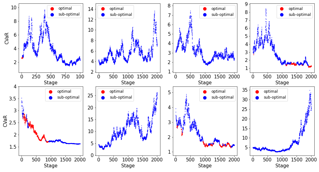
Figure 1: Evolution of the loss distribution CVaR_0.9 for all arms in a simulated run.

Notes: Each panel exhibits the evolution of the loss distribution CVaR_0.9 for one of the eight arms over the 2,000 stages in a single simulated run. The red color denotes the arm that is optimal (i.e. having the smallest CVaR_0.9) on a given stage.

First, to assess the impact of the choice of the step size $\lambda$ within the dual recursive estimation method or the weight exponential decay rate $\lambda$ in the weighted empirical estimation, a sensitivity analysis is conducted by comparing the time-$T$ (i.e. final) performance metrics for various choices of $\lambda$. Results are provided in Figure 2. Note that the set of generated losses over all arms and stages in a given run (i.e. $\{Y_{t,i}\}^{T}_{t=1}$, $i=1,\ldots,8$) is shared by the different values of $\lambda$ and the different estimation methods to reduce the impact of randomness when comparing the performance of different methods and hyperparameters.

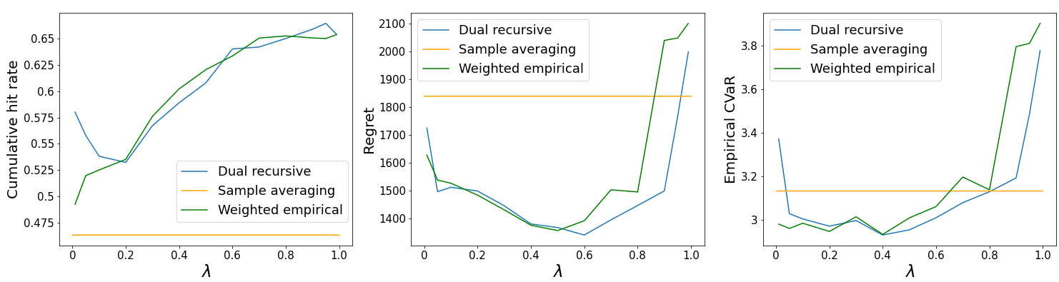
Figure 2: Performance versus parameter $\lambda$ (averaged over 1000 runs)

Notes: Time-$T$ performance metrics are reported for various choices of the parameter $\lambda$ for the three estimation methods under the slowly-varying loss distributions experiment detailed in Section 4.3. Parameter $\lambda$ corresponds to an exponential weight decay rate for the weighted empirical estimation, and to a learning rate for the dual recursive estimation. The orange curve corresponds to the sample averaging method (2), the green curve to the weighted empirical estimation method (4), and the blue curve to the dual recursive approach (7). Left panel: cumulative hit rate $\mathcal{H}_{t}$. Middle panel: average regret $\bar{\mathcal{R}}_{t}$. Right panel: empirical CVaR $\mathcal{C}_{t}$.

The orange curve representing the sample averaging method is flat since such method does not depend on any step size related parameter $\lambda$. For both the dual recursive and weighted empirical estimation methods, values around $\lambda=0.5$ seem to provide near-optimal results with respect to the regret and empirical CVaR performance metrics, and good results for the cumulative hit rate. Such value $\lambda=0.5$ is therefore retained for further tests. Compared to values often used in traditional reinforcement learning algorithms, the step size $\lambda=0.5$ could be considered quite large. The good performance associated with such value in the present framework is potentially due to the following: (i) there are not many observations available in the tail of the distribution for each arm, and thus extreme risk quantification requires larger step sizes associated with quicker and stronger updates, and (ii) non-stationarities require the use of larger step sizes than in stationary problems to put larger emphasis on most recent losses.

The performance of the three algorithms with a step size of $\lambda=0.5$ is now compared. The various performance metrics are reported in Figure 3 for all stages $t$ and all three estimation algorithms.

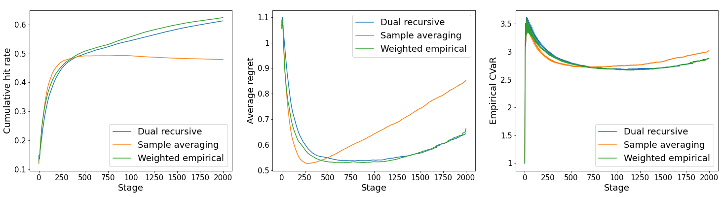
Figure 3: Evolution of performance metrics over time stages $t$ with $\lambda=0.5$ (averaged over 1000 runs)

Notes: Time-$t$ performance metrics are reported over the various stages $t$ for the three estimation methods under the slowly-varying loss distributions experiment detailed in Section 4.3. The orange curve corresponds to the sample averaging method (2), the green curve to the weighted empirical estimation method (4), and the blue curve to the dual recursive approach (7). Left panel: cumulative hit rate $\mathcal{H}_{t}$. Middle panel: average regret $\bar{\mathcal{R}}_{t}$. Right panel: empirical CVaR $\mathcal{C}_{t}$.

The weighted averaging (green curve) and dual recursive (blue curve) algorithms clearly outperform the sample averaging (orange curve) in the long run, which is not surprising given the presence of non-stationary losses. Moreover, the performance of the dual recursive approach and the weighted averaging approach is quite similar. Nevertheless, the ability to use the dual recursion formula on-line without needing to store all observed losses can compel a user to use this method for problems with a large number of stages requiring a quick implementation.

5 Conclusion

The present paper is the first to introduce action selection methods in the context of non-stationary risk averse multi-armed bandits problems. The objective function considered is the CVaR. Two approaches for its estimation on the various arms are proposed in the context of non-stationarity, one relying on a weighted empirical distribution of losses, and another based on the dual representation of the CVaR involving a recursive update formula. Such recursive formula is convenient if the multi-armed bandits problem is applied in an on-line setting, as it can be paralellized and it does not require storing the history of incurred losses for all arms. Conversely, the approach based on the weighted loss distributions possesses the advantage of not depending on arbitrary initial estimates. The proposed methods are benchmarked against a sample averaging estimator for the CVaR disregarding the potential non-stationary nature of loss distributions within an exploratory simulation experiments with slowly evolving loss distributions. The experiment reveals that the two proposed methods clearly outperform the naive sample averaging benchmark when losses are non-stationary. Moreover, the optimal step size $\lambda$ in the dual recursive estimation update formula (or alternatively the optimal weight decay parameter $\lambda$ in the weighted empirical estimation) is quite large, much above values that are often considered in a stationary case where the objective function is the expectation. Finally, for a suitably chosen parameter $\lambda$, the two non-stationary estimation methods seem to produce similar performance, without one clearly dominating the other.

As future research, it could be interesting to see if extreme value theory (see for instance McNeil et al.,, 2015) could be used in the context of non-stationary risk averse bandits when confidence levels close to one are considered. Such an approach is applied in the context of stationary bandits in Troop et al., (2019), but its extension to the non-stationary case might be non-trivial. Time varying thresholds in the peaks-over-threshold approach as in Kyselỳ et al., (2010) could be contemplated as method to tackle this problem. Furthermore, a second interesting research avenue would be the derivation of concentration bounds on CVaR estimates based on assumptions limiting the magnitude of loss distributions fluctuations.

References

- Baudry et al., (2021) Baudry, D., Gautron, R., Kaufmann, E., and Maillard, O. (2021). Optimal Thompson Sampling strategies for support-aware CVaR bandits. In International Conference on Machine Learning, pages 716–726. PMLR.
- Bouneffouf and Rish, (2019) Bouneffouf, D. and Rish, I. (2019). A survey on practical applications of multi-armed and contextual bandits. arXiv preprint arXiv:1904.10040.
- Brown, (2007) Brown, D. B. (2007). Large deviations bounds for estimating conditional value-at-risk. Operations Research Letters, 35(6):722–730.
- Cassel et al., (2018) Cassel, A., Mannor, S., and Zeevi, A. (2018). A general approach to multi-armed bandits under risk criteria. In Conference On Learning Theory, pages 1295–1306. PMLR.
- Chang et al., (2020) Chang, J. Q., Zhu, Q., and Tan, V. Y. (2020). Risk-constrained Thompson Sampling for CVaR bandits. arXiv preprint arXiv:2011.08046.
- Galichet et al., (2013) Galichet, N., Sebag, M., and Teytaud, O. (2013). Exploration vs exploitation vs safety: Risk-aware multi-armed bandits. In Asian Conference on Machine Learning, pages 245–260. PMLR.
- Godin, (2016) Godin, F. (2016). Minimizing CVaR in global dynamic hedging with transaction costs. Quantitative Finance, 16(3):461–475.
- Kagrecha et al., (2020) Kagrecha, A., Nair, J., and Jagannathan, K. (2020). Statistically robust, risk-averse best arm identification in multi-armed bandits. arXiv preprint arXiv:2008.13629.
- Khajonchotpanya et al., (2021) Khajonchotpanya, N., Xue, Y., and Rujeerapaiboon, N. (2021). A revised approach for risk-averse multi-armed bandits under CVaR criterion. Operations Research Letters, 49(4):465–472.
- (10) Kolla, R. K., Jagannathan, K., et al. (2019a). Risk-aware multi-armed bandits using conditional value-at-risk. arXiv preprint arXiv:1901.00997.
- (11) Kolla, R. K., Prashanth, L., Bhat, S. P., and Jagannathan, K. (2019b). Concentration bounds for empirical conditional value-at-risk: The unbounded case. Operations Research Letters, 47(1):16–20.
- Kyselỳ et al., (2010) Kyselỳ, J., Picek, J., and Beranová, R. (2010). Estimating extremes in climate change simulations using the peaks-over-threshold method with a non-stationary threshold. Global and Planetary Change, 72(1-2):55–68.
- Maillard, (2013) Maillard, O.-A. (2013). Robust risk-averse stochastic multi-armed bandits. In International Conference on Algorithmic Learning Theory, pages 218–233. Springer.
- McNeil et al., (2015) McNeil, A. J., Frey, R., and Embrechts, P. (2015). Quantitative risk management: concepts, techniques and tools-revised edition. Princeton university press.
- Newey and Powell, (1987) Newey, W. K. and Powell, J. L. (1987). Asymmetric least squares estimation and testing. Econometrica: Journal of the Econometric Society, pages 819–847.
- Prashanth et al., (2020) Prashanth, L., Jagannathan, K. P., and Kolla, R. K. (2020). Concentration bounds for CVaR estimation: The cases of light-tailed and heavy-tailed distributions. In ICML, pages 5577–5586.
- Rockafellar and Uryasev, (2002) Rockafellar, R. T. and Uryasev, S. (2002). Conditional value-at-risk for general loss distributions. Journal of Banking & Finance, 26(7):1443–1471.
- Sani et al., (2012) Sani, A., Lazaric, A., and Munos, R. (2012). Risk-aversion in multi-armed bandits. In Advances in Neural Information Processing Systems, pages 3275–3283.
- Sutton and Barto, (1998) Sutton, R. S. and Barto, A. G. (1998). Introduction to reinforcement learning, volume 135. MIT press Cambridge.
- Trindade et al., (2007) Trindade, A. A., Uryasev, S., Shapiro, A., and Zrazhevsky, G. (2007). Financial prediction with constrained tail risk. Journal of Banking & Finance, 31(11):3524–3538.
- Troop et al., (2019) Troop, D., Godin, F., and Yu, J. Y. (2019). Risk-averse action selection using extreme value theory estimates of the CVaR. arXiv preprint arXiv:1912.01718.
- Troop et al., (2021) Troop, D., Godin, F., and Yu, J. Y. (2021). Bias-corrected peaks-over-threshold estimation of the CVaR. arXiv preprint arXiv:2103.05059.
- Wang and Gao, (2010) Wang, Y. and Gao, F. (2010). Deviation inequalities for an estimator of the conditional value-at-risk. Operations Research Letters, 38(3):236–239.
- Yu and Nikolova, (2013) Yu, J. Y. and Nikolova, E. (2013). Sample complexity of risk-averse bandit-arm selection. In IJCAI, pages 2576–2582.