Constructing Prediction Intervals Using the Likelihood Ratio Statistic

Statistical prediction plays an important role in many decision processes such as university budgeting (depending on the number of students who will enroll), capital budgeting (depending on the remaining lifetime of a fleet of systems), the needed amount of cash reserves for warranty expenses (depending on the number of warranty returns), and whether a product recall is needed (depending on the number of potentially life-threatening product failures). In statistical inference, likelihood ratios have a long history of use for decision making relating to model parameters (e.g., in evidence-based medicine and forensics). We propose a general prediction method, based on a likelihood ratio (LR) involving both the data and a future random variable. This general approach provides a way to identify prediction interval methods that have excellent statistical properties. For example, if a prediction method can be based on a pivotal quantity, our LR-based method will often identify it. For applications where a pivotal quantity does not exist, the LR-based method provides a procedure with good coverage properties for both continuous or discrete-data prediction applications.

1 Introduction

1.1 Background

Prediction is a fundamental part of statistical inference. Prediction intervals are important for assessing the uncertainty of future random variables and have applications in business, engineering, science, and other fields. For example, manufacturers require prediction intervals for the number of warranty claims to assure that there are sufficient cash reserves and spare parts to make repairs; engineers use historical data to compute prediction intervals for the remaining lifetime of systems.

Suppose that the available data are denoted by $\boldsymbol{X}_{n}$, and that we want to predict a random variable denoted by $Y$ (also known as the predictand). We use a parametric distribution to model the data and the predictand. Specifically, we consider the case where $\boldsymbol{X}_{n}=\{X_{1},\dots,X_{n}\}$ corresponds to a sample of $n$ independent and identically distributed random variables with common density/mass function $f(\cdot;\boldsymbol{\theta})$. The density $f(\cdot;\boldsymbol{\theta})$ depends on a vector $\boldsymbol{\theta}$ of unknown parameters. The predictand $Y$ is a scalar random variable with conditional density $g(\cdot|\boldsymbol{x}_{n};\boldsymbol{\theta})$, where $\boldsymbol{X}_{n}=\boldsymbol{x}_{n}$ is the observed sample. If $Y$ is independent of $\boldsymbol{X}_{n}$, then $g(\cdot|\boldsymbol{x}_{n};\boldsymbol{\theta})=g(\cdot;\boldsymbol{\theta})$; further if $Y$ has the same distribution as the data, then $g(\cdot;\boldsymbol{\theta})=f(\cdot;\boldsymbol{\theta})$. The goal is to obtain information about the unknown parameters $\boldsymbol{\theta}$ from the data $\boldsymbol{X}_{n}$ to construct a prediction interval for the predictand $Y$.

We use $\text{PI}_{1-\alpha}(\boldsymbol{X}_{n})$ to denote a prediction interval for $Y$ with a nominal confidence level of $1-\alpha$. Letting $\Pr_{\boldsymbol{\theta}}(\cdot|\boldsymbol{X}_{n})$ be conditional probability given $\boldsymbol{X}_{n}$, the conditional coverage probability of $\text{PI}_{1-\alpha}(\boldsymbol{X}_{n})$ is

$$\text{CP}[\text{PI}_{1-\alpha}(\boldsymbol{X}_{n})|\boldsymbol{X}_{n}]=\Pr{}_{\!\boldsymbol{\theta}}\left[Y\in\text{PI}_{1-\alpha}(\boldsymbol{X}_{n})|\boldsymbol{X}_{n}\right].$$

We can obtain the unconditional coverage probability by taking the expectation of the conditional coverage probability $\text{CP}[\text{PI}_{1-\alpha}(\boldsymbol{X}_{n})|\boldsymbol{X}_{n}]$ with respect to $\boldsymbol{X}_{n}$,

$$\text{CP}[\text{PI}_{1-\alpha}(\boldsymbol{X}_{n})]=\Pr{}_{\!\boldsymbol{\theta}}[Y\in\text{PI}_{1-\alpha}(\boldsymbol{X}_{n})]=\text{E}_{\boldsymbol{\theta}}\left\{\text{CP}[\text{PI}_{1-\alpha}(\boldsymbol{X}_{n})|\boldsymbol{X}_{n}]\right\}.$$

Unlike the conditional coverage probability, which is a random variable, the unconditional coverage probability is a fixed property of a prediction interval procedure. Hence, the unconditional coverage probability is used to evaluate a prediction interval method and the term “coverage probability” is used to denote the unconditional coverage probability unless stated otherwise. If $\text{CP}[\text{PI}_{1-\alpha}(\boldsymbol{X}_{n})]=1-\alpha$, we say the prediction method is exact; if $\text{CP}[\text{PI}_{1-\alpha}(\boldsymbol{X}_{n})]\to 1-\alpha$ as $n\to\infty$, we say the prediction method is asymptotically correct.

1.2 Related Literature

Some prediction interval methods are based on a pivotal or an approximate pivotal quantity. The main idea is to find a function of $\boldsymbol{X}_{n}$ and $Y$, say $q(\boldsymbol{X}_{n},Y)$, that has a distribution that is free of parameters $\boldsymbol{\theta}$ (or approximately so for large samples). Then, the distribution of $q(\boldsymbol{X}_{n},Y)$ can be used to construct a $1-\alpha$ prediction region for $Y$ as

$$\mathcal{P}_{1-\alpha}(\boldsymbol{x}_{n})=\left\{y:q(\boldsymbol{x}_{n},y)\leq q_{n,1-\alpha}\right\},$$

where $\boldsymbol{X}_{n}=\boldsymbol{x}_{n}$ denotes the observed value of sample and $q_{n,1-\alpha}$ is the $1-\alpha$ quantile of $q(\boldsymbol{X}_{n},Y)$ (i.e., $\Pr{}_{\!\boldsymbol{\theta}}\left[q(\boldsymbol{X}_{n},Y)\leq q_{n,1-\alpha}\right]=1-\alpha$). If $q(\boldsymbol{x}_{n},y)$ is a monotone function of $y$, then $\mathcal{P}_{1-\alpha}(\boldsymbol{x}_{n})$ provides a one-sided prediction bound; if $-q(\boldsymbol{x}_{n},y)$ is a unimodal function of $y$, then $\mathcal{P}_{1-\alpha}(\boldsymbol{x}_{n})$ becomes a (two-sided) prediction interval. Relevant references of this pivotal method include Cox, (1975), Atwood, (1984), Beran, (1990), Barndorff-Nielsen and Cox, (1996), Nelson, (2000), Lawless and Fredette, (2005), and Fonseca et al., (2012).

One implementation of the pivotal method is through a hypothesis test. Cox, (1975) and Cox and Hinkley, (1979, Page 243) suggested to construct prediction intervals by inverting a hypothesis test, and gave examples with distributions having simple test statistics. Suppose the data $\boldsymbol{X}_{n}$ and the predictand $Y$ have densities $f(\boldsymbol{x}_{n};\boldsymbol{\theta})$ and $g(y;\boldsymbol{\theta}^{\dagger})$ governed by real-valued $\boldsymbol{\theta}$ and $\boldsymbol{\theta}^{\dagger}$, respectively, and a hypothesis test can be found for the null hypothesis $\boldsymbol{\theta}=\boldsymbol{\theta}^{\dagger}$. Let $w_{\alpha}$ be a critical region for the test $H_{0}:\boldsymbol{\theta}=\boldsymbol{\theta}^{\dagger}$ with size $\alpha$. For critical region $\omega_{\alpha}$ we have the probability statement

$$\Pr\left[(\boldsymbol{X}_{n},Y)\in w_{\alpha}\right]=\alpha.$$

Then for $\boldsymbol{X}_{n}=\boldsymbol{x}_{n}$, a $1-\alpha$ prediction region for $Y$ can be defined as

$$\mathcal{P}_{1-\alpha}(\boldsymbol{x}_{n})=\{y:(\boldsymbol{x}_{n},y)\not\in w_{\alpha}\}.$$ (1)

Thus, for the critical region defined in (1), we have that for all $\boldsymbol{\theta}$

$$\Pr{}_{\!\boldsymbol{\theta}}\left[Y\in\mathcal{P}_{1-\alpha}(\boldsymbol{X}_{n})\right]=1-\alpha,$$

so that (1) defines an exact prediction procedure for $Y$. In (1), one could also potentially use a critical region $w_{\alpha}\equiv w_{\alpha,n}$ having size $\alpha$ asymptotically (i.e., $\lim_{n\to\infty}\Pr_{\theta}\left[(\boldsymbol{X}_{,}Y)\in w_{\alpha}\right]=\alpha$); then (1) becomes an asymptotically correct $1-\alpha$ prediction region for $Y$.

Cox and Hinkley, (1979, pp. 245) illustrated this test-based prediction region (1) with the normal distribution. Suppose $\boldsymbol{X}_{n}$ is an independent random sample from $\text{Norm}(\mu,\sigma)$ and $Y$ is a further independent random variable with the same distribution. By assuming that $\boldsymbol{X}_{n}\sim\text{N}(\mu_{1},\sigma)$ and $Y\sim\text{N}(\mu_{2},\sigma)$, a test statistic for the null hypothesis $H_{0}:\mu_{1}=\mu_{2}$ is

$$t=\frac{\bar{X}_{n}-Y}{s\sqrt{(n+1)/n}}\sim t_{n-1},$$ (2)

where $s^{2}=\sum_{i=1}^{n}(X_{i}-\bar{X}_{n})^{2}/(n-1)$ and $t_{n-1}$ denotes a $t$-random variable with $n-1$ degrees of freedom. This corresponds to the form of a two-sample $t$-test that is often used for comparison of means. Then a $1-\alpha$ equal-tailed (i.e., equal probability of being outside either endpoint) prediction interval based on inverting the $t$-test is

$$\text{PI}_{1-\alpha}(\boldsymbol{X}_{n})=\left[\bar{X}_{n}-t_{n-1,\alpha/2}s\sqrt{(n+1)/n},\,\bar{X}_{n}+t_{n-1,\alpha/2}s\sqrt{(n+1)/n}\right],$$

where $t_{n-1,\alpha}$ denotes the $\alpha$ quantile of a $t_{n-1}$ distribution.

As a contrast to the pivotal prediction method, Bjørnstad, (1990) reviewed an alternative prediction method called the predictive likelihood method. The main idea of the predictive likelihood method is to obtain an approximate density for $Y$ by eliminating the unknown parameters in the joint likelihood (or density) of the data and the predictand $(\boldsymbol{X}_{n},Y)$. The resulting predictive likelihood then provides a type of distribution for computing a prediction interval for $Y$ given $\boldsymbol{X}_{n}=\boldsymbol{x}_{n}$. For example, a Bayesian predictive distribution for $Y$ involves steps of integrating out the unknown parameters of a posterior distribution based on the joint likelihood of the data and the predictand.

1.3 Motivations

As reviewed in Section 1.2, prediction intervals can be constructed by inverting hypothesis tests for parameters. However, the construction of such tests often needs to be tailored to each problem, where the determination of an appropriate hypothesis test is an essential step in the construction of such prediction intervals. For example, in the normal distribution example, we obtain the prediction interval by inverting a $t$-test. However, in many cases, there is no well-known or clear hypothesis test, making it difficult to implement a test-based method for obtaining prediction intervals. As a remedy, the purpose of this paper is to propose a general prediction method based on inverting a type of LR test. The advantage of the LR approach is that this principle applies broadly to different settings where prediction intervals are needed—and particularly for cases where an appropriate test statistic or pivotal quantity is not available or obvious for the need. In addition, we will demonstrate that this general method has desirable statistical properties.

1.4 Overview

This paper is organized as follows. Sections 2–5 focus on predictions with continuous data. Section 2 describes how to construct a prediction interval by formulating a certain LR statistic. Section 3 discusses situations where the proposed prediction method provides exact coverage, while Section 4 shows that, more broadly, that the method is generally (under weak conditions) guaranteed to provide asymptotically correct coverage (i.e., improving coverage properties with increasing sample sizes). Section 5 discusses some further details about constructing a suitable LR test. Section 6 focuses on applying the proposed method to prediction problems involving discrete data. Section 7 describes how the proposed LR prediction method compares and differs from predictions based on predictive likelihood methods (mentioned in Section 1.2). Section 8 concludes by describing potential areas for future research.

2 A General Method

In Section 2.1, we show how to construct general (not necessarily equal-tailed) two-sided prediction intervals with an LR statistic. Section 2.2 describes how to construct one-sided prediction intervals by using an LR and how this method can also be applied to calibrate equal-tailed two-sided prediction intervals. In this section, we assume that both the data $\boldsymbol{X}_{n}$ and the predictand $Y$ are continuous. For clarity in the exposition and ease of presentation, we further assume that $Y\sim g(\cdot;\boldsymbol{\theta})$ is independent of $\boldsymbol{X}_{n}\sim f(\cdot;\boldsymbol{\theta})$ and has the same distribution/density (i.e., $g(\cdot;\boldsymbol{\theta})=f(\cdot;\boldsymbol{\theta})$).

2.1 Prediction Intervals Based on an LR Test

Nelson, (2000) proposed a prediction interval method for predicting the number of failures in a future inspection of a sample of units, based on a likelihood ratio test in combination with the Wilks’ theorem. Although Nelson, (2000) only considered a specific prediction problem, we extend the principle of LR-based prediction interval statistics to a more general setting. The approach may also be viewed as a generalization of test-based prediction intervals explained in Cox and Hinkley, (1979), using an LR in the role of the test statistic.

2.1.1 Reduced and Full Models

Recalling its traditional use for parametric inference, the LR test provides a general approach for comparing two nested models for data (or parameter configurations) based on the observed data $\boldsymbol{X}_{n}=\boldsymbol{x}_{n}$. The null hypothesis about the parameters corresponds to a reduced model, which is nested within a larger full model (i.e., a parameter subset of the full model). Let $\mathcal{L}_{n}(\boldsymbol{\theta};\boldsymbol{x}_{n})$ be the likelihood function for the full model having a parameter space $\Theta$ and suppose that the reduced model (corresponding to the null hypothesis) has a constrained parameter space $\Theta_{0}\subset\Theta$. The LR for testing the null hypothesis $H_{0}:\boldsymbol{\theta}\in\Theta_{0}$ is then

$$\Lambda_{n}=\frac{\sup_{\boldsymbol{\theta}\in\Theta_{0}}\mathcal{L}_{n}(\boldsymbol{\theta};\boldsymbol{x}_{n})}{\sup_{\boldsymbol{\theta}\in\Theta}\mathcal{L}_{n}(\boldsymbol{\theta};\boldsymbol{x}_{n})},$$

and the log-LR statistic is $-2\log\Lambda_{n}$. Generally, the distribution of $\Lambda_{n}$ or $-2\log\Lambda_{n}$ needs to be determined, either analytically, through approximate large-sample distributional results, or through Monte Carlo simulation. Then, such a distribution can be used to determine the critical region for the LR test of the null hypothesis or relatedly a confidence interval/region for parameters. For example, if the reduced model is true, and if Wilks’ theorem (cf. Wilks, (1938)) applies (as it does under particular regularity conditions), the asymptotic distribution of the log-LR statistic is given by $-2\log\Lambda_{n}\xrightarrow{d}\chi^{2}_{d}$ as the sample size $n\to\infty$, where $\chi_{d}^{2}$ denotes a chi-square random variable with $d$ degrees of freedom and where $d$ is the difference in the lengths of $\Theta$ and $\Theta_{0}$. The latter large sample chi-square distribution approximation is often used to calibrate the critical region of an LR test.

As we describe next, a log-LR statistic for model parameters can be modified to provide a log-LR statistic for a future random variable $Y$ in a general manner, which in turn can be used to construct prediction intervals for $Y$. To outline the approach, suppose the available $\boldsymbol{X}_{n}$ represent an iid sample with common density $f(\cdot;\boldsymbol{\theta})$ and $Y$ denotes a future random variable with the same density $f(\cdot;\boldsymbol{\theta})$ ($Y$ is again independent of $\boldsymbol{X}_{n}$ here). A log-LR statistic for $Y$ can then be broadly framed as a type of parameter $\boldsymbol{\theta}$ comparison involving full vs reduced models for the joint distribution $(\boldsymbol{X}_{n},Y)$. While $f(\cdot;\boldsymbol{\theta})$ denotes the true marginal density for both the data $\boldsymbol{X}_{n}$ and the predictand $Y$ (with parameter space $\boldsymbol{\theta}\in\Theta$), the main idea is to define a hypothesis test regarding an enlarged (and fictional) parameter space $\Theta_{E}\equiv\{(\boldsymbol{\theta},\boldsymbol{\theta_{y}})\}$, where the data $X_{n}$ have a common density $f(\cdot;\boldsymbol{\theta})$, where the predictand $Y$ has a density $f(\cdot;\boldsymbol{\theta}_{y})$, say, and where $\boldsymbol{\theta}$ and $\boldsymbol{\theta}_{y}$ differ in exactly one pre-selected component when $(\boldsymbol{\theta},\boldsymbol{\theta}_{y})\in\Theta_{E}$. For example, supposing $\boldsymbol{\theta}=(\theta_{1},\ldots,\theta_{k})\in\Theta$ consists of $k\geq 1$ components, then we choose exactly one parameter component, say $\theta_{\ell}$, from among $\{\theta_{1},\ldots,\theta_{k}\}$ to vary and subsequently define $\boldsymbol{\theta}_{y}\in\Theta$ to match $\boldsymbol{\theta}\in\Theta$, except for the component $\ell$, which is $\theta_{\ell}$ for $\boldsymbol{\theta}$ but $\theta_{\ell,y}$ say in $\boldsymbol{\theta}_{y}$. This framework sets up a comparison of a contrived full model ($\boldsymbol{X}_{n}\sim f(\cdot;\boldsymbol{\theta})$ marginally and $Y\sim f(\cdot;\boldsymbol{\theta}_{y})$ for ($\boldsymbol{\theta},\boldsymbol{\theta}_{y})\in\Theta_{E}$) versus a reduced model ($\boldsymbol{\theta}_{y}=\boldsymbol{\theta}\in\Theta$), where the parameter space of the reduced model is nested within $\Theta_{E}$ with the constraint $\boldsymbol{\theta}=\boldsymbol{\theta}_{y}$.

The purpose of this contrived LR test is not to conduct hypothesis tests of parameters—as we already know that the reduced model is a true model—but to construct a predictive root (i.e., a test statistic containing $\boldsymbol{X}_{n}$ and $Y$), which will be used to predict $Y$. In particular, the extra degree of freedom between the parameter spaces of the full model and the reduced model is used to identify the predictand $Y$ when formulating a log-LR statistic for $\boldsymbol{\theta}=\boldsymbol{\theta}_{y}$. For example, in the case of data from a normal distribution $\boldsymbol{X}_{n},Y\sim\text{Norm}(\mu,\sigma)$, we may define a full model as $\boldsymbol{X}_{n}\sim\text{Norm}(\mu,\sigma)$ and $Y\sim\text{Norm}(\mu_{y},\sigma)$ for parameters $\boldsymbol{\theta}=(\mu,\sigma)$ and $\boldsymbol{\theta}_{y}=(\mu_{y},\sigma)\in\mathbb{R}\times(0,\infty)$, where the reduced model $\boldsymbol{\theta}_{y}=\boldsymbol{\theta}$ corresponds to the true underlying model $\boldsymbol{X}_{n},Y\sim\text{Norm}(\mu,\sigma)$ in prediction.

Let the joint likelihood function for $(\boldsymbol{X}_{n},Y)$ be

$$\mathcal{L}(\boldsymbol{\theta},\boldsymbol{\theta}_{y};\boldsymbol{x}_{n},y)=f(y;\boldsymbol{\theta}_{y})\prod_{i=1}^{n}f(x_{i};\boldsymbol{\theta})$$

under the full model and suppose the maximum likelihood (ML) estimators of $(\boldsymbol{\theta},\boldsymbol{\theta}_{y})$ are estimable under both the reduced ($\boldsymbol{\theta}=\boldsymbol{\theta}_{y}$) and the full ($(\boldsymbol{\theta},\boldsymbol{\theta}_{y})\in\Theta_{E}$) models. Then the joint LR statistic based on $(\boldsymbol{X}_{n},Y)$ is

$$\Lambda_{n}(\boldsymbol{X}_{n},Y)=\frac{\sup_{\boldsymbol{\theta}=\boldsymbol{\theta}_{y}\in\Theta}\mathcal{L}(\boldsymbol{\theta},\boldsymbol{\theta}_{y};\boldsymbol{X}_{n},Y)}{\sup_{(\boldsymbol{\theta},\boldsymbol{\theta}_{y})\in\Theta_{E}}\mathcal{L}(\boldsymbol{\theta},\boldsymbol{\theta}_{y};\boldsymbol{X}_{n},Y)}$$ (3)

for the test of $\boldsymbol{\theta}=\boldsymbol{\theta}_{y}$. The LR statistic in (3) and its distribution can then be applied to obtain prediction intervals for the future predictand $Y$ based on observed data values $\boldsymbol{X}_{n}=\boldsymbol{x}_{n}$. Note that the construction (3) depends on which parameter from $\boldsymbol{\theta}$ is selected to vary in defining $\boldsymbol{\theta}_{y}$. Typically, this selected parameter will be a mean-type parameter for purposes of identifying $Y$ in the LR statistic (3); more details about this selection are given in Section 5.

2.1.2 Determining the Distribution of the LR

The next step is to determine a critical region as in (1) so that we can compute the prediction region for $Y$, based on the LR statistic $\Lambda_{n}(\boldsymbol{X}_{n},Y)$ from (3). This, however, requires the distribution of $\Lambda_{n}(\boldsymbol{X}_{n},Y)$ (or $-2\log\Lambda_{n}(\boldsymbol{X}_{n},Y)$). There are three potential approaches for determining or approximating the distribution of $-2\log\Lambda_{n}(\boldsymbol{X}_{n},Y)$.

The first approach is to obtain the distribution of $-2\log\Lambda_{n}(\boldsymbol{X}_{n},Y)$ analytically. For illustration, consider the situation with an iid sample $\boldsymbol{X}_{n}\sim\text{Norm}(\theta,\sigma)$ where $\sigma$ is known and the future random variable $Y$ is from the same distribution. Here there is one parameter $\theta\equiv\mu$ where the full model is $\boldsymbol{X}_{n}\sim\text{Norm}(\mu,\sigma)$ and $Y\sim\text{Norm}(\mu_{y},\sigma)$ for $(\mu,\mu_{y})\in\mathbb{R}^{2}$ in the LR construction of (3); the corresponding log-LR statistic for $Y$ based on $\boldsymbol{X}_{n}$ is then

$$-2\log\Lambda_{n}(\boldsymbol{X}_{n},Y)=\frac{n}{n+1}\left(\frac{Y-\bar{X}_{n}}{\sigma}\right)^{2}\sim\chi^{2}_{1}.$$

Then, a $1-\alpha$ prediction region for $Y$ given $\boldsymbol{X}_{n}=\boldsymbol{x}_{n}$ is

$$\begin{split}\mathcal{P}_{1-\alpha}(\boldsymbol{x}_{n})&=\left\{y:-2\log\Lambda_{n}(\boldsymbol{x}_{n},y)\leq\chi^{2}_{1,1-\alpha}\right\}\\ &=\left\{y:\bar{x}_{n}-\sigma\sqrt{\frac{n+1}{n}\chi^{2}_{1,1-\alpha}}\leq y\leq\bar{x}_{n}+\sigma\sqrt{\frac{n+1}{n}\chi^{2}_{1,1-\alpha}}\right\}\\ &=\left\{y:\bar{x}_{n}-z_{1-\alpha/2}\sigma\sqrt{\frac{n+1}{n}}\leq y\leq\bar{x}_{n}+z_{1-\alpha/2}\sigma\sqrt{\frac{n+1}{n}}\right\}\end{split}$$

where $\chi_{1,1-\alpha}^{2}$ is the $1-\alpha$ quantile of $\chi^{2}_{1}$ and $z_{1-\alpha/2}=\sqrt{\chi^{2}_{1,1-\alpha}}$ is the $1-\alpha/2$ quantile of a standard normal variable. In this example, because $-2\log\Lambda_{n}(\boldsymbol{X}_{n},Y)$ is a unimodal function of $Y$, the prediction region $\mathcal{P}_{1-\alpha}(\boldsymbol{x}_{n})$ leads to a prediction interval and the LR prediction method has exact coverage probability because the log-LR statistic is a pivotal quantity (i.e., $\chi_{1}^{2}$-distributed).

The second approach for approximating the distribution of $-2\log\Lambda_{n}(\boldsymbol{X}_{n},Y)$, when applicable, is to use Wilks’ theorem. Under the conditions given in Wilks, (1938), the LR statistic $-2\log\Lambda_{n}(\boldsymbol{X}_{n},Y)\xrightarrow{d}\chi_{d}^{2}$, where $d$ is the difference in the dimensions of the full and reduced models ($d=1$ in our prediction interval construction). Similarly, the $1-\alpha$ prediction region based on Wilks’ theorem is

$$\mathcal{P}_{1-\alpha}(\boldsymbol{x}_{n})=\left\{y:-2\log\Lambda_{n}(\boldsymbol{x}_{n},y)\leq\chi^{2}_{d,1-\alpha}\right\}.$$

Wilks’ theorem, however, does not apply in all prediction problems. There exist important cases, particularly with discrete data, where the Wilks’ result is valid for the log-LR statistic $-2\log\Lambda_{n}(\boldsymbol{X}_{n},Y)$ in prediction and the chi-square-calibrated prediction region above is then appropriate; this is described in Section 6. When Wilks’ theorem does not apply, an alternative limiting distribution may still exist as illustrated in Section 4.

The third approach, which is the most general one, is to use parametric bootstrap. If $\lambda_{1-\alpha}$ is the $1-\alpha$ quantile of $\Lambda_{n}(\boldsymbol{X}_{n},Y)$, then we have the following prediction region

$$\mathcal{P}_{1-\alpha}(\boldsymbol{x}_{n})=\left\{y:-2\log\Lambda_{n}(\boldsymbol{x}_{n},y)\leq\lambda_{1-\alpha}\right\}.$$

The idea of this approach is to use a parametric bootstrap re-creation of the data $(\boldsymbol{X}_{n}^{*},Y^{*})$, which leads to a distribution for a bootstrap version $-2\log\Lambda_{n}(\boldsymbol{X}_{n}^{*},Y^{*})$ of the log-LR statistic. Then, the $1-\alpha$ quantile of the bootstrap distribution, say $\lambda_{1-\alpha}^{*}$, is used to approximate the unknown quantile $\lambda_{1-\alpha}$ of the true sampling distribution of $-2\log\Lambda_{n}(\boldsymbol{X}_{n},Y)$. Then the resulting parametric bootstrap prediction region is

$$\mathcal{P}_{1-\alpha}(\boldsymbol{x}_{n})=\left\{y:-2\log\Lambda_{n}(\boldsymbol{x}_{n},y)\leq\lambda_{1-\alpha}^{\ast}\right\}.$$ (4)

An algorithm for implementing a Monte Carlo (i.e., simulation-based) approximation of the parametric bootstrap is as follows.

1. Compute an estimate corresponding to a consistent estimator of $\boldsymbol{\theta}$ (usually the ML estimate) using observed data $\boldsymbol{X}_{n}=\boldsymbol{x}_{n}$, denoted by $\widehat{\boldsymbol{\theta}}_{n}$ (recall the data model is that the $\boldsymbol{X}_{n}$ are iid $f(\cdot;\boldsymbol{\theta})$.)

2. Generate a bootstrap sample $\boldsymbol{x}_{n}^{\ast}$ and $y^{\ast}$ as iid observations drawn from $f(\cdot;\widehat{\boldsymbol{\theta}})$.

3. Evaluate the LR in (3) using bootstrap pair $(\boldsymbol{x}_{n}^{\ast},y^{\ast})$ to get $\lambda^{\ast}\equiv-2\log\Lambda_{n}(\boldsymbol{x}_{n}^{\ast},y^{\ast})$.

4. Repeat steps 2–3 $B$ times to obtain $B$ realizations of $\lambda^{\ast}$ as $\{\lambda^{\ast}_{b}\}_{b=1}^{B}$.

5. Use the $1-\alpha$ sample quantile of $\{\lambda^{\ast}_{b}\}_{b=1}^{B}$ as $\lambda_{1-\alpha}^{\ast}$ in (4) and compute the prediction region.

The prediction region $\mathcal{P}_{1-\alpha}(\boldsymbol{x}_{n})$ in (4) is a prediction interval when $\Lambda_{n}(\boldsymbol{x}_{n},y)$ is a unimodal function of $y$ for a given data set $\boldsymbol{X}_{n}=\boldsymbol{x}_{n}$.

Such prediction intervals generally do not have equal-tail probabilities. In many applications, however, the cost of the predictand being greater than the upper bound is different than having it being less than the lower bound. In such cases, it is better to have a prediction interval with equal-tail probabilities. This can be achieved by calibrating separately the lower and upper one-sided $1-\alpha/2$ prediction bounds and putting them together to provide a two-sided $1-\alpha$ equal-tail-probability prediction interval. The next section shows how to construct a one-sided prediction bound using the LR in (3).

2.2 Constructing One-Sided Prediction Bounds

Suppose that the LR $\Lambda_{n}(\boldsymbol{x}_{n},y)$ is a unimodal function of $y$ based on observed data $\boldsymbol{X}_{n}=\boldsymbol{x}_{n}$. This is a common property (holding with probability 1) in most prediction problems. Note that a two-sided prediction interval (4) for $Y$ based on $\boldsymbol{X}_{n}=\boldsymbol{x}_{n}$ is defined by a horizontal line drawn through the curve of $-2\log\Lambda_{n}(\boldsymbol{x}_{n},y)$ (as a function of $y$) at an appropriate threshold $\lambda_{1-\alpha}$, as shown in Figure 1.

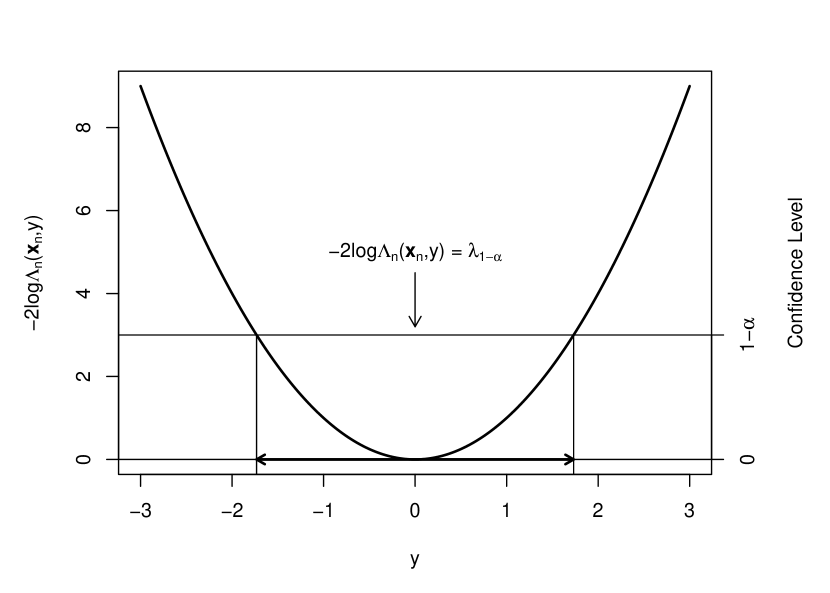
Figure 1: Example of log-LR statistic (as a function of $y$) for given data $\boldsymbol{x}_{n}$, which is an illustration of the prediction interval procedure in (4).

Here we describe a method for calibrating one-sided bounds directly, without resorting to (4) by adjusting the log-LR curve so that it becomes a monotone function. For a given data set $\boldsymbol{X}_{n}=\boldsymbol{x}_{n}$, let $y_{0}\equiv y_{0}(\boldsymbol{x}_{n})$ denote the value of $y$ that maximizes $\Lambda_{n}(\boldsymbol{x}_{n},y)$, where $\Lambda_{n}(\boldsymbol{x}_{n},y_{0})=1$ at $y_{0}$. Define a signed log-LR statistic $\zeta_{n}(\boldsymbol{x}_{n},y)$ based on (3) as

$$\zeta_{n}(\boldsymbol{x}_{n},y)\equiv(-1)^{\text{I}(y\leq y_{0})}\left[-2\log\Lambda_{n}(\boldsymbol{x}_{n},y)\right]=\left\{\begin{array}[]{ll}2\log\Lambda_{n}(\boldsymbol{x}_{n},y)\in(-\infty,0]&\mbox{$y\leq y_{0}$}\\ -2\log\Lambda_{n}(\boldsymbol{x}_{n},y)\in[0,\infty)&\mbox{$y\geq y_{0}$},\\ \end{array}\right.$$ (5)

where $\text{I}(\cdot)$ denotes the indicator function. That is, $(-1)^{\text{I}(y\leq y_{0})}\left[-2\log\Lambda_{n}(\boldsymbol{x}_{n},y)\right]$ is a signed version of the log-LR statistic $-2\log\Lambda_{n}(\boldsymbol{x}_{n},y)$ which, unlike the latter statistic, is an increasing function of $y$ and is negative when $y<y_{0}$ (but positive when $y>y_{0}$). Hence, to set a one-sided bound for $Y$, we calibrate the signed log-LR statistic $\zeta_{n}(\boldsymbol{x}_{n},y)$ which has a one-to-one correspondence to $y$-values when $\Lambda_{n}(\boldsymbol{x}_{n},y)$ is unimodal (unlike $\Lambda_{n}(\boldsymbol{x}_{n},y)$ itself).

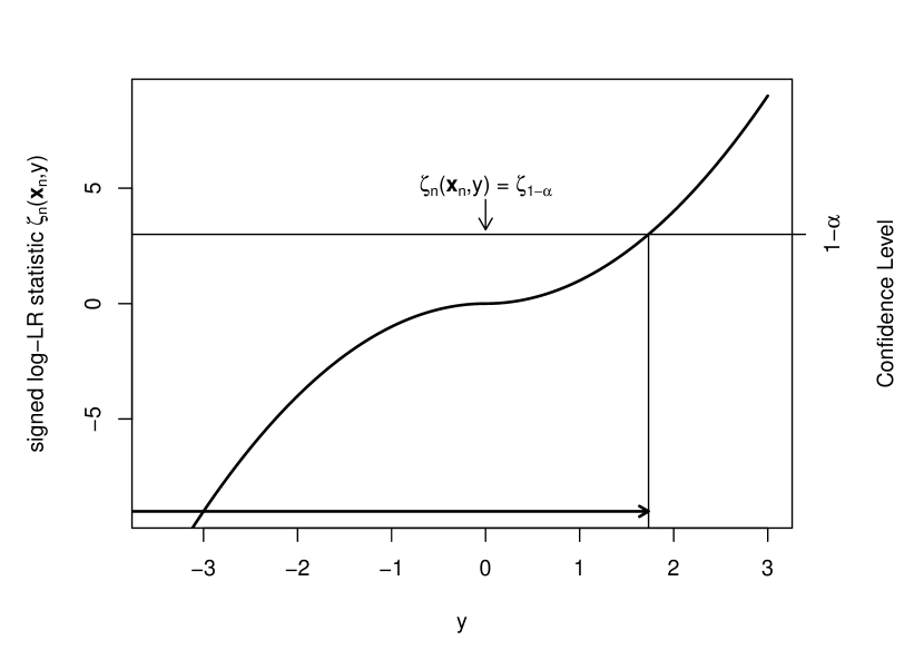
Figure 2: An illustration of the one-sided prediction bound procedure in (6).

Note that if the $1-\alpha$ quantile of the distribution of $\zeta_{n}(\boldsymbol{X}_{n},Y)$, denoted by $\zeta_{1-\alpha}$, were known, we could set a $1-\alpha$ upper prediction bound for $Y$ given $\boldsymbol{X}_{n}=\boldsymbol{x}_{n}$ as

$$\tilde{y}_{1-\alpha}(\boldsymbol{x}_{n})\equiv\sup\{y\in\mathbb{R}:\zeta_{n}(\boldsymbol{x}_{n},y)\leq\zeta_{1-\alpha}\}.$$ (6)

Figure 2 provides a graphical illustration of (6), illustrating the resulting prediction region. Similar to the third approach in Section 2.1.2, we can approximate the quantile $\zeta_{1-\alpha}^{\ast}$ using the $1-\alpha$ quantile of $\zeta_{n}(\boldsymbol{X}_{n}^{\ast},Y^{\ast})$, which is the bootstrap version of the signed log-LR statistic. Then, a bootstrap prediction bound is obtained by replacing $\zeta_{1-\alpha}$ with $\zeta_{1-\alpha}^{\ast}$ in (6), and the $1-\alpha$ upper prediction bound $\tilde{y}_{1-\alpha}(\boldsymbol{x}_{n})$ is defined as

$$\tilde{y}_{1-\alpha}(\boldsymbol{x}_{n})=\sup_{y\in\mathbb{R}}\left\{y:\zeta_{n}(\boldsymbol{x}_{n},y)\leq\zeta_{1-\alpha}^{\ast}\right\}.$$ (7)

Constructing the $1-\alpha$ lower prediction bound $\underaccent{\tilde}{y}_{1-\alpha}(\boldsymbol{x}_{n})$ is similar, and the $1-\alpha$ lower prediction bound is

$$\underaccent{\tilde}{y}_{1-\alpha}(\boldsymbol{x}_{n})=\sup_{y\in\mathbb{R}}\left\{y:\zeta_{n}(\boldsymbol{x}_{n},y)\leq\zeta_{\alpha}^{\ast}\right\}.$$ (8)

The following algorithm describes how to compute the $1-\alpha$ upper (and lower) prediction bound $\tilde{y}_{1-\alpha}(\boldsymbol{x}_{n})$ (and $\underaccent{\tilde}{y}_{\alpha}(\boldsymbol{x}_{n})$) using a Monte Carlo approximation of the bootstrap distribution $\zeta_{n}(\boldsymbol{X}_{n}^{\ast},Y^{\ast})$ and the bootstrap quantile $\zeta_{1-\alpha}^{\ast}$ (and $\zeta_{\alpha}^{\ast}$).

1. Compute $\widehat{\boldsymbol{\theta}}_{n}$ using the observed data $\boldsymbol{X}_{n}=\boldsymbol{x}_{n}$.

2. Simulate a sample $\boldsymbol{x}_{n}^{\ast}$ using a parametric bootstrap with $\widehat{\boldsymbol{\theta}}_{n}$ and compute $y_{0}(\boldsymbol{x}_{n}^{\ast})$.

3. Simulate $y^{\ast}$ from distribution $f(\cdot;\widehat{\boldsymbol{\theta}}_{n})$ and compute

   $$\zeta^{\ast}\equiv\zeta_{n}(\boldsymbol{x}_{n}^{\ast},y^{\ast})=(-1)^{\text{I}[y^{\ast}\leq y_{0}(\boldsymbol{x}_{n}^{\ast})]}\left[-2\log\Lambda_{n}(\boldsymbol{x}_{n}^{\ast},y^{\ast})\right].$$

4. Repeat steps 2–3 $B$ times to obtain $B$ realizations of $\zeta^{\ast}$ as $\{\zeta_{i}^{\ast}\}_{i=1}^{B}$.

5. Use the $1-\alpha$ (or $\alpha$) sample quantile from $\{\zeta_{i}^{\ast}\}_{i=1}^{B}$ as $\zeta_{1-\alpha}^{\ast}$ (or $\zeta_{\alpha}^{\ast}$) in (7) (or (8)) to compute the $1-\alpha$ upper (or lower) prediction bound.

Note that, in the algorithm for one-side bounds, one can simultaneously keep track of bootstrap statistics $\lambda^{\ast}=\left|\xi^{\ast}\right|$ for computing the two-sided bounds in (4) (i.e., the same resamples can be used).

3 Exact Results

The LR-based prediction method can often uncover and exploit pivotal quantities involving the data $\boldsymbol{X}_{n}$ and the predictand $Y$ when these exist. In these cases, the LR statistic is pivotal, often emerging as a function of another pivotal quantity from $(\boldsymbol{X}_{n},Y)$. Consequently, in these cases, prediction intervals or bounds for $Y$ based on the LR-statistic (3) will have exact coverage, when either based on the direct distribution of LR statistic (when available analytically) or more broadly when based on a bootstrap. In this section, we provide more explanation about when the LR prediction method is exact, beginning with some illustrative examples.

Exponential Distribution: Suppose the data $X_{1},\dots,X_{n}$ and future predictand $Y$ are iid $\text{Exp}(\theta)$ with mean $\theta>0$. Letting $\widehat{\theta}_{\boldsymbol{x}_{n},y}\equiv\left(\sum_{i=1}^{n}x_{i}+y\right)/(n+1)$, and $\widehat{\theta}_{\boldsymbol{x}_{n}}\equiv\sum_{i=1}^{n}x_{i}/n$ based on data $\boldsymbol{X}_{n}=\boldsymbol{x}_{n}$ and a given value $y>0$ of $Y$, then the LR statistic (3) is

$$\Lambda_{n}(\boldsymbol{x}_{n},y)=\frac{\widehat{\theta}^{-n-1}_{\boldsymbol{x}_{n},y}\exp\left[-\frac{\sum_{i=1}^{n}x_{i}+y}{\widehat{\theta}_{\boldsymbol{x}_{n},y}}\right]}{\widehat{\theta}_{\boldsymbol{x}_{n}}^{-n}\exp\left[-\frac{\sum_{i=1}^{n}x_{i}}{\widehat{\theta}_{\boldsymbol{x}_{n}}}\right]y^{-1}\exp\left(-\frac{y}{y}\right)}=\frac{y\widehat{\theta}_{\boldsymbol{x}_{n}}^{n}}{\widehat{\theta}_{\boldsymbol{x}_{n},y}^{n+1}}=\frac{\left(\frac{\bar{x}_{n}}{y}\right)^{n}}{\left[\frac{n}{n+1}\frac{\bar{x}_{n}}{y}+\frac{1}{n+1}\right]^{n+1}},$$

which is a function of the pivotal quantity $\bar{X}_{n}/Y$ and a unimodal function of $y$. Thus, the LR prediction method is exact (when based on the $F$-distribution of $\bar{X}_{n}/Y\sim F_{n,1}$ or the bootstrap as in (4)), and the prediction region becomes a prediction interval.

Normal Distribution: Let $X_{1},\dots,X_{n},Y\sim\text{Norm}(\mu,\sigma)$, where both $\mu\in\mathbb{R}$ and $\sigma>0$ are unknown. We construct the full model by allowing the predictand $Y$ to have a different location parameter $\mu$: $X_{1}\dots,X_{n}\sim\text{Norm}(\mu,\sigma)$ and $Y\sim\text{Norm}(\mu_{y},\sigma)$ (i.e., $\boldsymbol{\theta}=(\mu,\sigma)$ and $\boldsymbol{\theta}_{y}=(\mu_{y},\sigma)$). Then for the full model, the ML estimators are

$$\widehat{\mu}=\bar{X}_{n},\quad\widehat{\mu}_{y}=Y,\quad\widehat{\sigma}=\sqrt{\frac{\sum_{i=1}^{n}(X_{i}-\bar{X}_{n})^{2}}{n+1}},$$

while for the reduced model $\theta=\theta_{y}$, the ML estimators are

$$\widehat{\mu}=\frac{\sum_{i=1}^{n}X_{i}+Y}{n+1},\quad\widehat{\sigma}=\sqrt{\frac{\sum_{i=1}^{n}(X_{i}-\widehat{\mu})^{2}+(Y-\widehat{\mu})^{2}}{n+1}}.$$

Then the resulting LR statistic (3) is

$$\Lambda_{n}(\boldsymbol{X}_{n},Y)=\left(1+\frac{n^{2}+1}{n^{2}-1}\frac{t^{2}}{n}\right)^{-(n+1)/2}$$ (9)

where

$$t\equiv\frac{\bar{X}_{n}-Y}{s}\sqrt{\frac{n}{n+1}},$$

and $s^{2}\equiv\sum_{i=1}^{n}(X_{i}-\bar{X}_{n})^{2}/(n-1)$. Here, $t\sim t_{n-1}$ has the same $t$-test statistic form as in (2). Hence, the LR is pivotal and also $\Lambda_{n}(\boldsymbol{x}_{n},y)$ is a unimodal function of $y$. Thus the resulting prediction interval procedure has exact coverage probability when based on the bootstrap as in (4) (or using the $t_{n-1}$ distribution here).

In fact, the results for the normal distribution can be generalized to the (log-)location-scale family, which contains many other important distributions. Theorem 1 says that, by allowing the location parameter of the predictand to be different from that of the data to create a full versus reduced model comparison, the resulting LR statistic (3) is a pivotal quantity so that the prediction method is exact.

Theorem 1.

(i) Suppose the LR-statistic (3) is a pivotal quantity. Then, the corresponding $1-\alpha$ prediction region (4) for $Y$ based on the parametric bootstrap will have exact coverage. That is,

$$\Pr\left[Y\in\mathcal{P}_{1-\alpha}(\boldsymbol{X}_{n})\right]=1-\alpha.$$

(ii) Suppose also that both the data $X_{1},\dots,X_{n}$ and $Y$ are from a location-scale distribution with density $f(\cdot;\mu,\sigma)=\phi\left[(x-\mu)/\sigma\right]$ with parameters $\boldsymbol{\theta}=(\mu,\sigma)\in\mathbb{R}\times(0,\infty)$. In the LR construction (3), suppose the full model involves parameters $\boldsymbol{\theta}=(\mu,\sigma)$ and $\boldsymbol{\theta}_{y}=(\mu_{y},\sigma)$ (i.e., $X_{1},\dots,X_{n}\sim f(\cdot;\mu,\sigma)$ and $Y\sim f(\cdot;\mu_{y},\sigma)$). Then the LR statistic $\Lambda_{n}(\boldsymbol{X}_{n},Y)$ (or $-2\log\Lambda_{n}(\boldsymbol{X}_{n},Y)$) is a pivotal quantity and the result of Theorem 1(i) holds.

The proof is given in Section A of supplementary material.

Remark 1. If the LR statistic $\Lambda_{n}(\boldsymbol{x}_{n},y)$ is a unimodal function of $y\in\mathbb{R}$ with probability 1 (as determined by $\boldsymbol{X}_{n}$) and if the signed LR-statistic $\zeta_{n}(\boldsymbol{X}_{n},Y)$ is a pivotal quantity, then the Theorem 1(i) result (i.e., exact coverage) also applies for one-sided prediction bounds based on parametric bootstrap. For (log-)location-scale distributions as in Theorem 1(ii), the signed LR-statistic $\zeta_{n}(\boldsymbol{X}_{n},Y)$ is a pivot.

We next provide some illustrative examples.

Simple Regression: We consider the simple linear regression model $Y\sim\text{Norm}(\beta_{0}+\beta_{1}x,\sigma)$ with given $x$ and data $Y_{1},\dots,Y_{n}$ that satify $Y_{i}\sim\text{Norm}(\beta_{0}+\beta_{1}x_{i},\sigma)$ where $x_{i},i=1,\dots,n$. Similar to the normal distribution example, it is natural to choose $\beta_{0}+\beta_{1}x$ to construct the “full” model. In fact, choosing $\beta_{0}$ or $\beta_{1}$ gives the same log-LR statistic as $\beta_{0}+\beta_{1}x$, which is given by

$$(n+1)\log\left(1+\frac{1}{n-2}T^{2}\right),$$

where $T$ matches the standard statistic for normal theory predictions (i.e., a studentized version of $Y-\widehat{\beta}_{0}-\widehat{\beta}_{1}x$) having a $t$-distribution with $n-2$ degrees of freedom.

Two-Parameter Exponential Distribution: Suppose $X_{1},\dots,X_{n},Y$ are independent observations from a two-parameter exponential distribution $\text{Exp}(\mu,\beta)$. That is, $(X_{i}-\mu)/\beta\sim\text{Exp}(1)$ with location and scale parameters as $\boldsymbol{\theta}=(\mu,\beta)$. Hence, under Theorem 1, the LR $\Lambda_{n}(\boldsymbol{X}_{n},Y)$ is a pivotal quantity and bootstrap-calibrated prediction regions for $Y$ are exact. In fact, an exact form of the LR-statistic may be determined as

$$\Lambda_{n}(\boldsymbol{x}_{n},y)=\left[\frac{\sum_{i=1}^{n}x_{i}+y-(n+1)\min\{x_{(1)},y\}}{\sum_{i=1}^{n}x_{i}-nx_{(1)}}\right]^{n+1}$$

based on given positive data $\boldsymbol{x}_{n}=(x_{1},\ldots,x_{n})$ where $x_{(1)}$ denotes the first order statistic. Note that $\Lambda_{n}(\boldsymbol{x}_{n},y)$ is a unimodal function of $y$ given $\boldsymbol{X}_{n}=\boldsymbol{x}_{n}$ (with probability 1); hence, one-sided prediction bounds for $Y$ based on a parametric bootstrap will also have exact coverage by Remark 1. Replacing $\boldsymbol{x}_{n}$ and $y$ with corresponding random variables $\boldsymbol{X}_{n}$ and $Y$ in (3) gives

$$\Lambda_{n}(\boldsymbol{X}_{n},Y)\stackrel{{\scriptstyle d}}{{=}}\left[\frac{\sum_{i=1}^{n}E_{i}+T-(n+1)\min\{E_{(1)},T\}}{\sum_{i=1}^{n}E_{i}-nE_{(1)}}\right]^{n+1},$$

where $E_{1},\dots,E_{n},T$ denote iid $\text{Exp}(1)$ random variables and $E_{(1)}$ is the first order statistic of $E_{1},\dots,E_{n}$; this verifies that $\Lambda_{n}(\boldsymbol{X}_{n},Y)$ is indeed a pivotal quantity for the exponential data case, as claimed in Theorem 1. Thus this prediction interval procedure is exact when parametric bootstrap is used to obtain the distribution of $\Lambda_{n}(\boldsymbol{X}_{n},Y)$.

Uniform Distribution: Suppose $X_{1},\dots,X_{n},Y$ are iid $\text{Unif}(0,\theta)$, which is a one-parameter scale family. The LR statistic (3) has a form

$$\Lambda_{n}(\boldsymbol{x}_{n},y)=\frac{(x_{(n)}/y)^{n}}{[\max(x_{(n)}/y,1)]^{n+1}},$$ (10)

where $x_{(n)}$ denotes the maximum of $\{x_{1},\dots,x_{n}\}$. Hence, $\lambda_{n}(\boldsymbol{x}_{n},y)$ is a unimodal function $y$ given $\boldsymbol{X}_{n}=\boldsymbol{x}_{n}$ (with probability 1) and $\Lambda_{n}(\boldsymbol{X}_{n},Y)$ can also be seen to be a pivotal quantity as

$$\frac{X_{(n)}}{Y}=\frac{X_{(n)}/\theta}{Y/\theta}\stackrel{{\scriptstyle d}}{{=}}\frac{\max\{U_{1},\dots,U_{n}\}}{U_{0}},$$

where $U_{0},U_{1},\dots,U_{n}$ denote iid $\text{Unif}(0,1)$ variables. Hence, by Theorem 1(i) and Remark 1, both the two-sided prediction interval procedure (4) as well as the one-sided bound procedures (7)-(8) based on bootstrap have exact coverage. That is, bootstrap simulation provides an effective and unified means for estimating the distribution of $\Lambda_{n}(\boldsymbol{x}_{n},y)$ and constructing prediction intervals.

4 General Results

Section 3 discusses cases where the LR prediction method is exact, particularly when the construction (3) results in a pivotal quantity. For some prediction problems, however, the LR statistic may not be a pivotal quantity, as the next example illustrates.

Gamma Distribution: Let $X_{1},\dots,X_{n},Y$ denote iid random variables from a gamma density $f(x;\alpha,\beta)=\beta^{-\alpha}x^{\alpha-1}\exp(-x/\beta)/{\Gamma(\alpha)}$, $x>0$, with scale $\beta>0$ and shape $\alpha>0$ parameters. In the LR construction (3) with parameters $\boldsymbol{\theta}=(\beta,\alpha)$, suppose the full model involves parameters $\boldsymbol{\theta}$ and $\boldsymbol{\theta}_{y}=(\beta_{y},\alpha)$ or $X_{1},\dots,X_{n}\sim\text{Gamma}(\alpha,\beta)$ and $Y\sim\text{Gamma}(\alpha,\beta_{y})$. The LR statistic is then given by

$$\Lambda_{n}(\boldsymbol{x}_{n},y)=\frac{\sup_{\alpha}[\Gamma(\alpha)]^{-n}[(n\bar{x}_{n}+y)/(n+1)]^{-\alpha(n+1)}(y\prod_{i=1}^{n}x_{i})^{\alpha-1}}{\sup_{\alpha}[\Gamma(\alpha)]^{-n}[n\bar{x}_{n}]^{-\alpha n}(y/\alpha)^{-\alpha}(y\prod_{i=1}^{n}x_{i})^{\alpha-1}}.$$

Unlike the previous examples, the LR statistic is no longer a pivotal quantity. However, we can use the bootstrap method to approximate the distribution for $\Lambda_{n}(\boldsymbol{X}_{n},Y)$. A small simulation study was conducted to investigate the coverage probability of the LR prediction method. Figure 3 shows the coverage probability of 90% and 95% one-sided prediction bounds for a future gamma variate based on the LR prediction method (i.e., (7) and (8)), and compares the LR prediction method with other methods. Sample size values $n=4,5,6,7,8,9,10,30,50,70,90,100$ were used. Without loss of generality, the scale parameter was set to $\beta=1$, and the shape parameter values $\alpha=1,2,3$ were used. $N=2000$ Monte Carlo samples were used to compute the coverage probability and $B=2000$ bootstrap samples were used to approximate the distribution of the signed log-LR statistic.

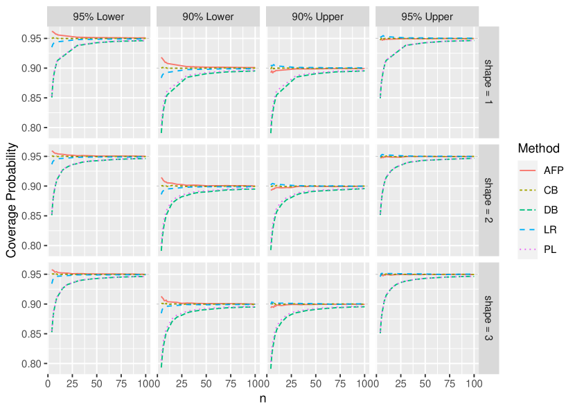
Figure 3: Coverage probabilities for predicting a gamma random variable versus the sample size $n$ for the $90\%$ and $95\%$ one-sided prediction bounds: Approximate Fiducial Prediction (AFP) (Chen and Ye, 2017), Calibration Bootstrap (CB) (Beran, 1990), Direct-Bootstrap (DB) (Harris, 1989), Likelihood Ratio Prediction (LR) (cf. (7), and (8)); Plug-in (PL) Methods.

The simulation results show that the calibration-bootstrap method has the best coverage while the LR prediction and the approximate fiducial (or GPQ) methods also work well. When $n=4$, the difference between the true coverage of the LR prediction method and the nominal level (combined with Monte Carlo error) is less than $2\%$. When the sample size $n$ increases, the discrepancy quickly shrinks. This illustrtates that even when the LR statistic has a complicated and non-pivotal distribution, using parameteric bootstrap can be effective and useful.

Theorem 2, given next, shows that the LR prediction method, combined with bootstrap calibration is asymptotically correct for continuous prediction problems under general conditions. The theorem consists of two parts: the first part establishes that the log-LR statistic $-2\log\Lambda_{n}(\boldsymbol{X}_{n},Y)$ has a limit distribution as $n\to\infty$. However, this limit distribution will sometimes not be chi-square as in Wilks’ theorem and may even depend on one or more of the parameters. Nevertheless, the second part of Theorem 2 establishes that the bootstrap version of the log-LR statistic $-2\log\Lambda_{n}(\boldsymbol{X}_{n}^{\ast},Y^{\ast})$ can capture the distribution of $-2\log\Lambda_{n}(\boldsymbol{X}_{n},Y)$. Consequently, $1-\alpha$ bootstrap-based prediction regions (4) for $Y$ will have coverage probabilities that converge to the correct coverage level $1-\alpha$ as the sample size $n$ increases.

Theorem 2.

Suppose a random sample $\boldsymbol{X}_{n}$ of size $n$ and a predictand $Y$ (independent of $\boldsymbol{X}_{n}$) have a common density $f(\cdot;\boldsymbol{\theta})$, and that the LR construction (3) is used with $\boldsymbol{\theta}=(\theta,\boldsymbol{\theta}^{\prime})$ and $\boldsymbol{\theta}_{y}=(\theta_{y},\boldsymbol{\theta}^{\prime})$ having common parameters $\boldsymbol{\theta}^{\prime}$ (and real-valued parameters $\theta,\theta_{y}$ that may differ). Then, under mild regularity conditions (detailed in the supplement),

1. As $n\to\infty$,

   $$-2\log\Lambda_{n}(\boldsymbol{X}_{n},Y)\xrightarrow{d}-2\log\left[\frac{f(Y;\boldsymbol{\theta}_{0})}{\sup_{\theta_{y}}f(Y;\theta_{y},\boldsymbol{\theta}_{0}^{\prime})}\right],$$

   where $\boldsymbol{\theta}_{0}=(\theta_{0},\boldsymbol{\theta}_{0}^{\prime})$ denotes the true value of the parameter vector $\boldsymbol{\theta}$.

2. The bootstrap provides an asymptotically consistent estimator of the distribution of the log-LR statistic; that is,

   $$\sup_{\lambda\in\mathbb{R}}\left|\Pr{}_{\!\ast}(-2\log\Lambda_{n}^{\ast}\leq\lambda)-\Pr\left(-2\log\Lambda_{n}\leq\lambda\right)\right|\xrightarrow{p}0,$$

   where $\Pr{}_{\!\ast}$ is the bootstrap induced probability and $\Lambda^{\ast}_{n}\equiv\Lambda_{n}(\boldsymbol{X}_{n}^{\ast},Y^{\ast})$.

Remark 2. Similar to Remark 1, if $\Lambda_{n}(\boldsymbol{X}_{n},y)$ is a unimodal function of $y$ (with probability 1 or with probability approaching 1 as $n\to\infty$), then the signed log-LR statistic converges as well

$$(-1)^{\text{I}[Y\leq y_{0}(X_{n})]}\left[-2\log\Lambda_{n}(\boldsymbol{X}_{n},Y)\right]\stackrel{{\scriptstyle d}}{{\rightarrow}}\begin{cases}2\log\left[\frac{f(Y;\boldsymbol{\theta}_{0})}{\sup_{\theta_{y}}f(Y;\theta_{y},\boldsymbol{\theta}^{\prime}_{0})}\right],&Y\leq m_{0}.\\ -2\log\left[\frac{f(Y;\boldsymbol{\theta}_{0})}{\sup_{\theta_{y}}f(Y;\theta_{y},\boldsymbol{\theta}^{\prime}_{0})}\right],&Y>m_{0}.\end{cases}$$

where $m_{0}$ is maximizer of ${f(y;\boldsymbol{\theta}_{0})}/{\sup_{\theta_{y}}f(y;\theta_{y},\boldsymbol{\theta}^{\prime}_{0})}$ over $y$. The bootstrap approximation for the signed log-LR statistic is also valid asymptotically. The proof is described in the supplementary material along with a proof of Theorem 2.

We use two examples to illustrate Theorem 2. In the uniform example of Section 3, if $\theta_{0}>0$ denotes the true parameter value (i.e., $Y\sim\mbox{Unif}(0,\theta_{0})$), then the limit distribution in Theorem 2(i) for the log-LR statistic is

$$-2\log\Lambda_{n}(\boldsymbol{X}_{n},Y)\xrightarrow{d}-2\log\left(\frac{Y}{\theta_{0}}\right),$$ (11)

which has a $\chi^{2}_{2}$ distribution. This result can be alternatively verified by using the LR in (10) to determine that

$$\Lambda_{n}(\boldsymbol{X}_{n},Y)=\frac{(X_{(n)}/Y)^{n}}{[\max(X_{(n)}/Y,1)]^{n+1}}=\frac{Y}{X_{(n)}}\frac{(X_{(n)}/Y)^{n+1}}{\left[\max(X_{(n)}/Y,1)\right]^{n+1}}\xrightarrow{d}\text{Unif}(0,1)$$

from which $-2\log\Lambda_{n}(\boldsymbol{X}_{n},Y)\xrightarrow{d}\chi_{2}^{2}$ follows. While $\Lambda_{n}(\boldsymbol{X}_{n},Y)$ is a pivotal quantity for any $n\geq 1$ (so that bootstrap calibration is exact by Theorem 1), Theorem 2 shows that the bootstrap also captures the limiting distribution of the log-LR statistic $\chi_{2}^{2}$ in (11).

To consider a distribution with more than one parameter, we re-visit the gamma distribution example in this section. Using Theorem 2, the limit distribution is

$$\begin{split}-2\log\Lambda_{n}(\boldsymbol{X}_{n},Y)&\xrightarrow{d}-2\log\left[\frac{f(Y;\beta_{0},\alpha_{0})}{\sup_{\beta}f(Y;\beta,\alpha_{0})}\right]\\ &=-2\log\left[\left(\frac{Y}{\beta_{0}}\right)^{\alpha_{0}}\exp\left(-\frac{Y}{\beta_{0}}+\alpha_{0}\right)\right]\\ &=2(Z-\alpha_{0})-2\alpha_{0}\log(Z),\end{split}$$ (12)

where $Z\equiv Y/\beta_{0}\sim\text{Gamma}(\alpha_{0},1)$. Even though the log-LR statistic (3) depends on the shape parameter $\alpha_{0}$ in this example, a bootstrap approximation for the distribution of the log-LR statistic is asymptotically correct by Theorem 2. This is demonstrated numerically through the coverage behavior of Figure 3.

In addition to the bootstrap (Theorem 2 (ii)), the limit distribution of the log-LR statistic in Theorem 2 (i) (as well as that of the signed log-LR statistic $\zeta_{n}$ from Remark 2) may also be used as an alternative approach to construct prediction intervals. That is, we may use the $1-\alpha$ quantile of the limit distribution in Theorem 2 (i) to replace the quantile $\lambda_{1-\alpha}$ in (4) (corresponding to the finite sampling distribution of the log-LR statistic). For example, in the uniform prediction example above, the limit distribution is $\chi_{2}^{2}$ from (11) and an approximate $1-\alpha$ prediction region for $Y$ would be $\{y:-2\log\Lambda_{n}(\boldsymbol{x}_{n},y)\leq\chi^{2}_{2,1-\alpha}\}$, which has asymptotically correct coverage by Theorem 2 (i). As another example from the gamma prediction case, we can use the $1-\alpha$ quantile of the limit distribution in (12) to replace $\lambda_{1-\alpha}$ in (4). This limit distribution, however, depends on the unknown shape parameter $\alpha_{0}$ in (12), which differs from the uniform case where the log-LR statistic has a limit distribution in (11) that is free of unknown parameters. However, in prediction cases such as the gamma distribution, where the limit distribution of log-LR statistic from Theorem 2 (i) does depend on unknown parameters, we can still approximate and use the limit distribution by replacing any unknown parameters with consistent estimators. To illustrate with gamma predictions, we may estimate the unknown shape parameter $\alpha_{0}$ in (12) with the ML estimate $\widehat{\alpha}$ from the data $\boldsymbol{X}_{n}=\boldsymbol{x}_{n}$ and compute the $1-\alpha$ quantile of the “plug-in” version of the limit distribution $2(Z-\widehat{\alpha})-2\widehat{\alpha}\log(Z)$. Such use of the limit distribution of the log-ratio statistic (Theorem 2 (i)), possibly with plug-in estimation, can be computationally simpler than parametric bootstrap and may have advantages for large sample sizes or when the numerical costs of repeated ML estimation (i.e., as in bootstrap) are prohibitive.

5 How to Choose the Full Model

When $\boldsymbol{\theta}$ is a parameter vector, construction of the LR statistic depends on which parameter component in $\boldsymbol{\theta}$ is varied to create $\boldsymbol{\theta}_{y}$ in a full model, where $(\boldsymbol{\theta},\boldsymbol{\theta}_{y})$ again differ in exactly one component. Our recommendation is to choose a parameter that is most readily identifiable from a single observation. In other words, we can envision maximizing $f(y|\boldsymbol{\theta})$, the density of one observation, with respect to a single unknown parameter of our choice, with all remaining parameters fixed at arbitrary values; the parameter that represents the simplest single maximization step of $f(y|\boldsymbol{\theta})$ corresponds to a good parameter choice in the LR construction and choosing such a parameter can simplify computation. Under some one-to-one reparameterization, if necessary, such a parameter is often given by the mean or the median of the model density $f(y|\boldsymbol{\theta})$ that can naturally be identified through a single observation $Y$. This approach is also supported by Theorem 2 where the limiting distribution of the LR statistic is determined by a single-parameter maximization. We provide some examples in the rest of this section.

Normal Distribution: For $\text{Norm}(\mu,\sigma)$ with unknown $\mu,\sigma$, consider maximizing the normal density $f(y;\mu,\sigma)$ of a single observation $Y$ with respect to one parameter while the other parameter is fixed. If choosing $\mu$, then we can estimate $\mu$ simply as $\widehat{\mu}_{y}=y$. However, if choosing $\sigma$, we have $\widehat{\sigma}_{y}^{2}=(y-\mu)^{2}$, which is less simple. More technically, the LR construction for the normal model then eventually involves a complicated estimation of the remaining parameter $\mu$ (from a “full” model sample $x_{1},\dots,x_{n},y$) as the maximizer of $-2\log|y-\mu|-n\log[\sum_{i=1}^{n}(x_{i}-\mu)^{2}]$, which can exhibit numerical sensitivity in the value of $y$. We have seen in Section 3 that choosing the mean parameter $\mu$ gives a LR statistic with a nice form and coverage properties, but choosing $\sigma$ results in a much less tractable LR statistic.

Gamma Distribution: For a gamma distribution with shape $\alpha$ and scale $\beta$, we select the parameter that most easily maximizes a single gamma density $f(y;\alpha,\beta)$ when the other parameter is fixed. Choosing $\beta$ is simpler than choosing $\alpha$ because the maximizer of the gamma pdf with respect to $\beta$ is $\widehat{\beta}=\alpha/y$ while choosing $\alpha$ does not yield a closed-form maximizer. Also, choosing $\alpha$ leads to a more complicated LR statistic and a less tractable limit distribution, from Theorem 2. Alternatively, to more closely align parameter choice in the gamma distribution with parameter identification from one observation, we use another parameterization $(\alpha\beta,\alpha)$ and choose the mean $\alpha\beta$ (i.e., estimated as $y$ analogously to the normal case). This choice will produce the same LR statistic as choosing $\beta$ in the parameterization $(\beta,\alpha)$. Hence, choosing a parameter with the simplest stand-alone maximization step in a parameterization and choosing a parameter based on identifiability considerations (e.g., means) in a second parameterization are related concepts.

Generalized Gamma Distribution: The (extended) generalized gamma distribution, using the Farewell and Prentice, (1977) parameterization (see also Section 4.13 of Meeker et al., 2021) has (on the log scale) a location $\mu$, a scale $\sigma$, and a shape parameter $\lambda$ with a pdf given by

$$f(y;\mu,\sigma,\lambda)=\begin{cases}\dfrac{|\lambda|}{\sigma y}\phi_{lg}[\lambda\omega+\log(\lambda^{-2});\lambda^{-2}]\quad&\text{if}\quad\lambda\neq 0\\ \dfrac{1}{\sigma y}\phi_{\text{norm}}(\omega)&\text{if}\quad\lambda=0,\end{cases}$$

where $y>0$, $\omega=[\log(y)-\mu]/\sigma$, $-\infty<\mu<\infty$, $-\infty<\lambda<\infty$, $\sigma>0$, $\phi_{\text{norm}}(\cdot)$ is the pdf of $\text{Norm}(0,1)$, and $\phi_{lg}(z;\kappa)=\exp\left[\kappa z-\exp(z)\right]/{\Gamma(\kappa)}$. When considering the maximization of a single density $f(y;\mu,\sigma,\lambda)$ for one of the three parameters (with others fixed), the ML estimator of $\mu$ has the simplest form as $\widehat{\mu}=\log(y)$. Hence, we choose $\mu$ to construct the “full” model. A small simulation study was done to investigate the coverage probability of one-sided prediction bounds. Fixing the location parameter at $\mu=0$ and the scale parameter at $\sigma=1$ without loss of generality, we consider four different levels for the shape parameter $\lambda=0.5,1,1.5,2$. The Monte Carlo sample size was set as $N=2000$; the bootstrap sample size was set as $B=2000$. The data sample sizes are $n=30,35,40,45,50,55,60,70,80,90,100$. Figure 4 shows the coverage probabilities for the LR prediction method and for the plug-in method (where the unknown parameters are replaced with the ML estimates) versus the sample size. We can see that the LR method has good coverage probability and consistently outperforms the plug-in method. Also, the coverage probability of the LR method, if not close to the nominal confidence level, is conservative. The plug-in method, however, is always anti-conservative in this simulation study.

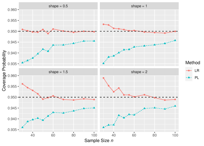
Figure 4: Coverage probabilities of 95% upper bounds using LR prediction method (LR) and naive plug-in method (PL) versus the sample size $n$.

6 Discrete Distributions

Prediction methods for discrete distributions are less well developed when compared to those for continuous distributions. Many methods (e.g., the calibration-bootstrap method proposed by Beran, 1990) that generally work in continuous settings are not applicable for certain discrete data models. This section presents three prediction applications based on discrete distributions and shows that the LR prediction method not only works for discrete distributions but also has performance comparable to existing methods that were especially tailored to these particular discrete prediction problems. Because the LR prediction method is a generally applicable method for prediction, the good performance of the method against specialized alternatives in these discrete cases is also suggestive that the LR approach may apply well in other prediction problems.

6.1 Binomial Distribution

We consider the prediction problem where there are two independent binomial samples with the same probability $p$. The initial sample $X$ has a distribution $\text{Binom}(n,p)$ and the predictand $Y$ has a distribution $\text{Binom}(m,p)$. Both $n$ and $m$ are known, and note here that the data and predictand have related, though not identical, distributions (unlike predictions in Sections 3-4 with continuous $Y$). The goal is to construct a prediction interval for $Y$ given observed data $X=x$.

Using the fact that the conditional distribution of $X$ given the sum $X+Y$ does not depend on the parameter $p$, Thatcher, (1964) proposed a prediction method based on the cdf of the hypergeometric distribution. Faulkenberry, (1973) proposed a similar method using the conditional distribution of $Y$ given the sum $X+Y$, which is also free of the parameter $p$. Nelson, (1982) proposed a different approach using the asymptotic normality of an approximate pivotal statistic. However, numerical studies in Wang, (2008) and Krishnamoorthy and Peng, (2011) showed that Nelson’s method has poor coverage probability, and proposed alternative prediction methods using asymptotic normality (e.g., based on inverting a score-like statistic instead of a Wald-like statistic).

To construct prediction intervals using the LR prediction method, the reduced model is that $X$ and $Y$ have the same parameter $p$ while the full model allows $X$ and $Y$ to have a different $p$ in the construction (3). The LR statistic is then

$$\Lambda_{n,m}(x,y)=\frac{\text{dbinom}(x,n,\widehat{p}_{xy})\times\text{dbinom}(y,m,\widehat{p}_{xy})}{\text{dbinom}(x,n,\widehat{p}_{x})\times\text{dbinom}(y,m,\widehat{p}_{y})}=\frac{(\widehat{p}_{xy})^{x+y}(1-\widehat{p}_{xy})^{n+m-x-y}}{(\widehat{p}_{x})^{x}(1-\widehat{p}_{x})^{n-x}(\widehat{p}_{y})^{y}(1-\widehat{p}_{y})^{m-y}},$$

where dbinom is the binomial pmf, $\widehat{p}_{x}=x/n$, $\widehat{p}_{y}=y/m$, and $\widehat{p}_{xy}=(x+y)/(n+m)$. The asymptotic distribution of the log-LR statistic is $-2\log\Lambda_{n,m}(X,Y)\xrightarrow{d}\chi^{2}_{1}$ as $n\to\infty$ and $m\to\infty$; this theoretical result is explained further in Section 6.4 for discrete data. The prediction region is defined as

$$\mathcal{P}_{1-\alpha}(x)=\{y:-2\log\Lambda_{n,m}(x,y)\leq\chi_{1,1-\alpha}^{2}\},$$ (13)

which gives an approximate $1-\alpha$ prediction interval procedure that has, asymptotically, equal-tail probabilities.

Due to the discrete nature of data here, we can further refine the LR prediction method by making a continuity correction at the extreme values $x=0$ or $x=n$ and $y=0$ or $y=m$. We first define $x^{\prime}\equiv x+0.5\text{I}_{x=0}-0.5\text{I}_{x=n}$ and $y^{\prime}\equiv y+0.5\text{I}_{y=0}-0.5\text{I}_{y=m}$ and further define $\widehat{p}^{\prime}_{x}\equiv x^{\prime}/n$, $\widehat{p}^{\prime}_{y}\equiv y^{\prime}/m$, and $\widehat{p}^{\prime}_{xy}\equiv(x^{\prime}+y^{\prime})/(n+m)$. The corrected LR statistic is then

$$\Lambda_{n,m}^{\prime}(x,y)=\frac{(\widehat{p}_{xy}^{\prime})^{x^{\prime}+y^{\prime}}(1-\widehat{p}_{xy}^{\prime})^{n+m-x^{\prime}-y^{\prime}}}{(\widehat{p}_{x}^{\prime})^{x^{\prime}}(1-\widehat{p}_{x}^{\prime})^{n-x^{\prime}}(\widehat{p}_{y}^{\prime})^{y^{\prime}}(1-\widehat{p}_{y}^{\prime})^{m-y^{\prime}}}.$$

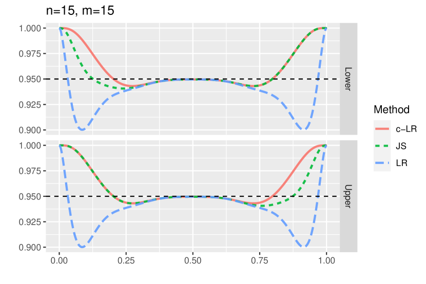
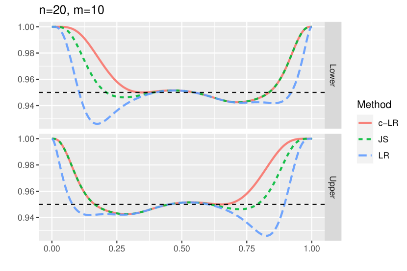
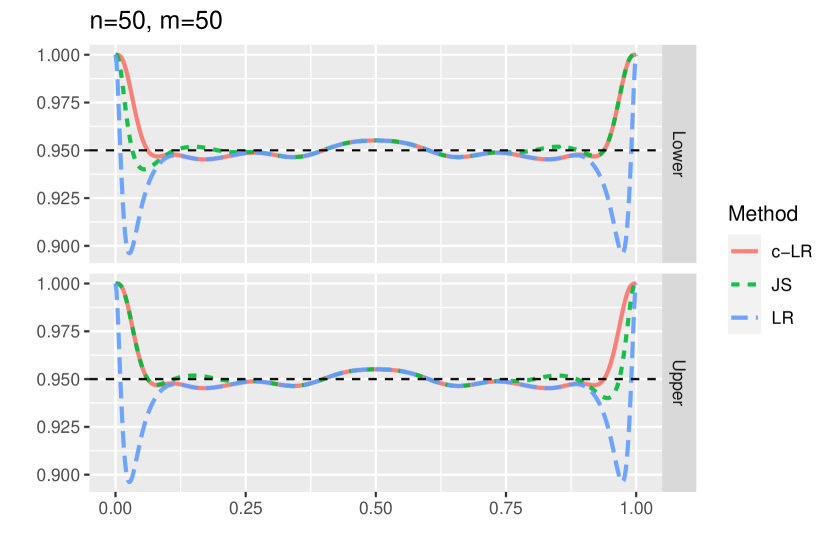
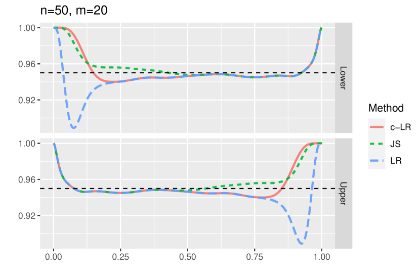
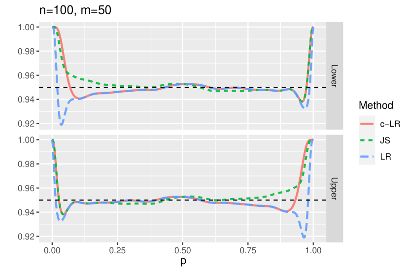
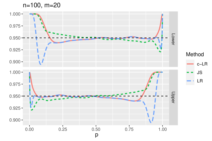
Figure 5: Coverage probabilities of 95% lower and upper prediction bounds using corrected LR prediction method (c-LR), joint sample prediction method (JS), and LR prediction method (LR) as a function of $p$.

A numerical study was done to investigate the coverage probability of the LR prediction methods and we also used the joint sampling prediction method as a benchmark for comparison because of its good coverage probability (cf. Krishnamoorthy and Peng, 2011). The results in Figure 5 show that the original LR prediction method can have poor coverage for small sample sizes (e.g., $n=15$) when $p$ is near 0 or 1. However, with the continuity correction, the coverage probability of the corrected LR prediction method is comparable to that of the joint sampling prediction method. Unlike the joint sampling prediction method though, the LR prediction method is a general approach, which applies outside binomial prediction problems and has not been specifically designed for this purpose. The numerical results here aim to provide evidence that the LR prediction method can be a generally effective procedure for prediction.

6.2 Poisson Distribution

Suppose $X\sim\text{Poi}(n\lambda)$ and $Y\sim\text{Poi}(m\lambda)$, where $n$ and $m$ are known positive integers and $\lambda>0$ is unknown. The goal is to construct prediction intervals for $Y$ based on data $X=x$. Similar to the binomial example, one can construct prediction intervals using the fact that the conditional distribution of $X$ or $Y$ given $X+Y$ is binomial while Nelson, (1982) and Krishnamoorthy and Peng, (2011) proposed alternative methods using a Wald-like approximate pivotal quantity.

To construct prediction intervals using the LR prediction method, the reduced model for the LR statistic (3) is that $X$ and $Y$ have the same $\lambda$ parameter while for the full model, $X$ and $Y$ may not have the same $\lambda$ parameter. The LR statistic is given by

$$\Lambda_{n,m}(x,y)=\frac{\text{dpois}(x,n\widehat{\lambda}_{xy})\times\text{dpois}(y,m\widehat{\lambda}_{xy})}{\text{dpois}(x,n\widehat{\lambda}_{x})\times\text{dpois}(y,m\widehat{\lambda}_{y})}=\frac{\exp\left[-(n+m)\widehat{\lambda}_{xy}\right](n\widehat{\lambda}_{xy})^{x}(m\widehat{\lambda}_{xy})^{y}}{\exp\left(-n\widehat{\lambda}_{x}-m\widehat{\lambda}_{y}\right)(n\widehat{\lambda}_{x})^{x}(m\widehat{\lambda}_{y})^{y}},$$

where $\widehat{\lambda}_{xy}=(x+y)/(n+m)$, $\widehat{\lambda}_{x}=x/n$, $\widehat{\lambda}_{y}=y/m$, and dpois is the Poisson pmf. The prediction interval can be obtained using the same procedure in (13); see Section 6.4 for justification. We can also refine the LR prediction method with a continuity correction at the extremes $x=0$ or $y=0$ by letting $x^{\prime}\equiv x+0.5\text{I}_{x=0}$ and $y^{\prime}\equiv y+0.5\text{I}_{y=0}$. Then define $\widehat{\lambda}_{xy}^{\prime}\equiv(x^{\prime}+y^{\prime})/(n+m)$, $\widehat{\lambda}^{\prime}_{x}\equiv x^{\prime}/n$, and $\widehat{\lambda}_{y}^{\prime}\equiv y^{\prime}/m$ so that the corrected LR statistic is

$$\Lambda_{n,m}^{\prime}(x,y)=\frac{\exp\left[-(n+m)\widehat{\lambda}_{xy}^{\prime}\right](n\widehat{\lambda}_{xy}^{\prime})^{x^{\prime}}(m\widehat{\lambda}_{xy}^{\prime})^{y^{\prime}}}{\exp\left(-n\widehat{\lambda}_{x}^{\prime}-m\widehat{\lambda}_{y}^{\prime}\right)(n\widehat{\lambda}_{x}^{\prime})^{x^{\prime}}(m\widehat{\lambda}_{y}^{\prime})^{y^{\prime}}}.$$

A numerical study was done to investigate the coverage probability of the proposed methods. Similar to the binomial example, the joint sampling method from Krishnamoorthy and Peng, (2011) was used for comparison because of its good coverage properties. Figure 6 shows that the continuity correction improves the poor coverage of the LR prediction method when $\lambda$ is small. The coverage probability of the corrected LR prediction method is comparable to that of the joint sampling method. In the bottom-right subplot of Figure 6, the corrected method has better performance than the joint sampling method. Again, unlike the joint sampling prediction method, the LR prediction method is general and not specifically designed for Poisson predictions.

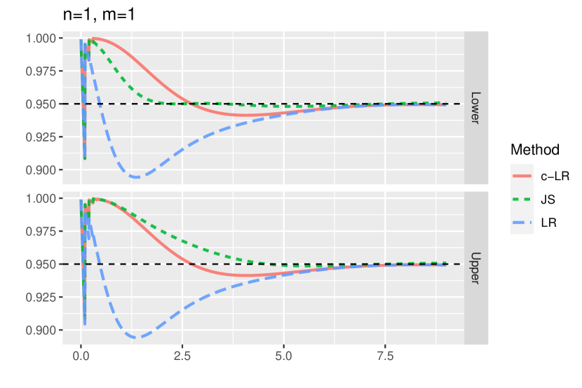
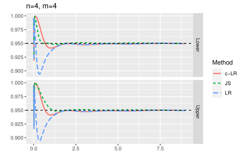
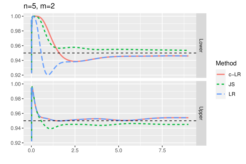
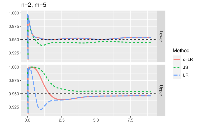
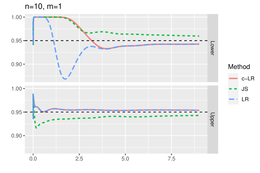
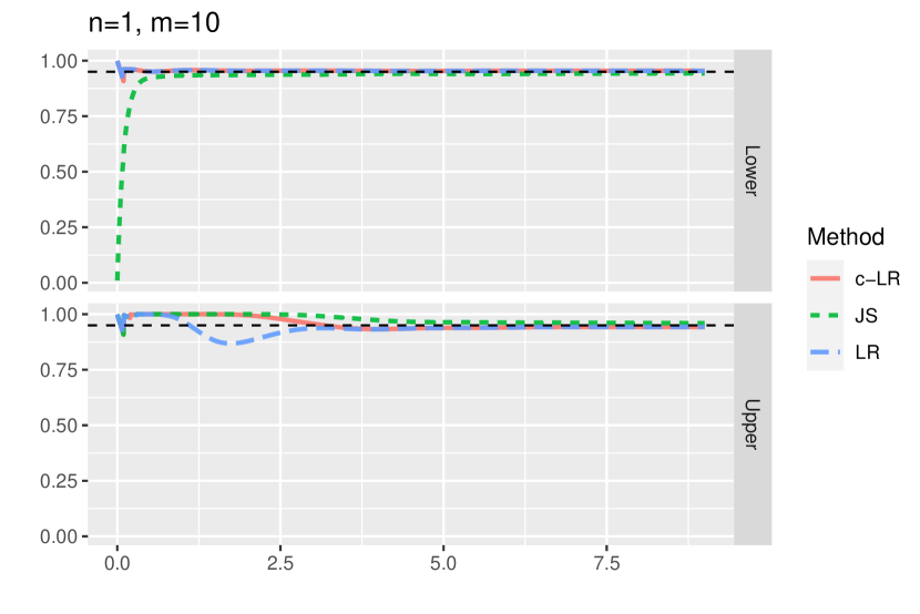
Figure 6: Coverage probabilities of 95% Poisson lower and upper prediction bounds using the corrected LR prediction method (c-LR), joint sample prediction method (JS), and LR prediction method (LR) as a function of $\lambda$.

6.3 Predicting the Number of Future Events

Suppose $n$ units start service at time $t=0$ and that the lifetime of each unit has a continuous parametric distribution with cdf $F(t;\boldsymbol{\theta})$ and density $f(t;\boldsymbol{\theta})$. At a data freeze date, the unfailed units have accrued $t_{c}$ time units of service (e.g., hours or months in service) while $r_{n}$ failures have occurred and the failure times (all less than $t_{c}$) are known. A prediction interval for the number of failures that will occur in the interval $(t_{c},t_{w}]$ $(t_{w}>t_{c},)$ is required. This problem is called within sample prediction because the predictand and the observed Type-I censored data are from the same sample. The within-sample prediction and related problems have been studied in Escobar and Meeker, (1999) using a calibration method. Similar problems have been studied in Nelson, (2000) and Nordman and Meeker, (2002) based on an LR statistic without calibration. Tian et al., (2020) showed that the simple plug-in method (where ML estimates replace the unknown parameters in the distribution of the predictand and the $\alpha/2$ and $1-\alpha/2$ quantiles of the resulting distribution define an approximate $1-\alpha$ prediction interval procedure) is not asymptotically correct and proposed three alternative methods, based on parametric bootstrap samples, that are asymptotically correct. In this paper, we propose another solution based on an LR statistic, that does not require bootstrap samples.

Suppose that a random sample $T_{1},\dots,T_{n}\sim F(t;\boldsymbol{\theta})$ is observed under Type-I censoring with $r_{n}=\sum_{i=1}^{n}\text{I}(T_{i}\leq t_{c})$ censored units (failures). The predictand is the number $Y=\sum_{i=1}^{n}\text{I}(t_{c}\leq T_{i}\leq t_{w})$ of events occurring in the future interval $(t_{c},t_{w}]$. For the $n-r_{n}$ units surviving at $t_{c}$, the conditional probability of each unit to fail in $(t_{c},t_{w}]$, given that the unit survived to $t_{c}$, is given by

$$p\equiv\Pr\left(t_{c}<T_{1}\leq t_{w}|T_{1}>t_{c}\right).$$ (14)

6.3.1 Implementing the LR Prediction Method

To implement the LR prediction method, we specify a reduced model versus full model comparison in order to construct an LR statistic analogous to (3). Such models will be formulated in terms of the value (14) of the conditional probability $p$ for the interval $(t_{c},t_{w}]$, recalling that the predictand $Y$ is the number of failures (out of $n-r_{n}$ possible) that will occur in this interval. For the reduced model, we assume that the time-to-failure process is governed by $F(t;\boldsymbol{\theta})$ in the interval $(0,t_{w}]$ and that the conditional probability (14) of a failure in $(t_{c},t_{w}]$ is

$$p=\frac{F(t_{w};\boldsymbol{\theta})-F(t_{c};\boldsymbol{\theta})}{1-F(t_{c};\boldsymbol{\theta})}.$$

The likelihood function for the reduced model is

$$\mathcal{L}_{1}(\boldsymbol{\theta};\boldsymbol{t}_{n},y)=\binom{n-r_{n}}{y}\prod_{i=1}^{r}f(t_{(i)};\boldsymbol{\theta})\left[F(t_{w};\boldsymbol{\theta})-F(t_{c};\boldsymbol{\theta})\right]^{y}\left[1-F(t_{w};\boldsymbol{\theta})\right]^{n-y-r_{n}}.$$ (15)

For the full model, $F(t;\boldsymbol{\theta})$ will still be the time-to-failure distribution in the interval $(0,t_{c}]$ but not $(t_{c},t_{w}]$, so that the value (14) of the conditional probability $p\in(0,1]$ becomes one additional parameter. The likelihood function for the full model is

$$\mathcal{L}_{2}(\boldsymbol{\theta},p;\boldsymbol{t}_{n},y)=\binom{n-r_{n}}{y}\prod_{i=1}^{r}f(t_{(i)};\boldsymbol{\theta})p^{y}(1-p)^{n-y-r_{n}}.$$ (16)

By maximizing the likelihood functions in (15) and (16), the LR statistic is

$$\Lambda_{n}(\boldsymbol{t}_{n},y)=\frac{\sup_{\boldsymbol{\theta}}L_{1}(\boldsymbol{\theta};\boldsymbol{t}_{n},y)}{\sup_{\boldsymbol{\theta},p}L_{2}(\boldsymbol{\theta},p;\boldsymbol{t}_{n},y)}.$$

The asymptotic (as $n\to\infty$) distribution of $-2\log\Lambda_{n}(\boldsymbol{T}_{n},Y)$ is $\chi_{1}^{2}$, because the full model has one more parameter than the reduced model and standard regularity conditions hold (see also Section 6.4). An approximate $1-\alpha$ prediction region is defined as

$$\{y:-2\log\Lambda_{n}(\boldsymbol{t}_{n},y)\leq\chi_{1,1-\alpha}^{2}\},$$ (17)

where $\chi_{1,1-\alpha}^{2}$ is the $1-\alpha$ quantile of the $\chi_{1}^{2}$ distribution. Because $\Lambda_{n}(\boldsymbol{t}_{n},y)$ is a unimodal function of $y$, the prediction region in (17) provides the desired approximate prediction interval.

6.3.2 A Simulation Study

A simulation study was done to examine the coverage probability of the LR prediction method for the within-sample prediction problem. We simulated Type-I censored data with censoring time $t_{c}$ using the Weibull distribution

$$F(t;\beta,\eta)=1-\exp\left[-\left(\frac{t}{\eta}\right)^{\beta}\right],\quad t>0.$$

Then we constructed prediction intervals for the number of failures in the future time interval $(t_{c},t_{w}]$ using several methods: plug-in, LR, direct-bootstrap, GPQ-bootstrap, and calibration-bootstrap methods. As mentioned earlier, the plug-in method, which replaces the unknown parameter $\boldsymbol{\theta}=(\beta,\eta)$ with a consistent estimate $\widehat{\boldsymbol{\theta}}_{n}$, fails to provide asymptotically correct prediction intervals (cf. Tian et al., 2020). The last three methods are from Tian et al., (2020) and have been established to be asymptotically correct.

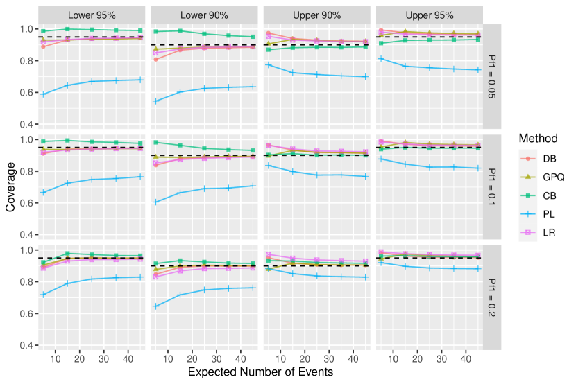
Figure 7: Coverage probabilities versus expected number of events (failures) for the direct-bootstrap (DB), GPQ-bootstrap (GPQ), calibration-bootstrap (CB), LR, and plug-in (PL) methods when $d=0.1$ and $\beta=2$.

The factors for this simulation study include

1. The probability that a unit fails before the censoring time $t_{c}$: $p_{f1}=F(t_{c};\beta,\eta)$.

2. The expected number of failures at the censoring time $t_{c}$: $\text{E}(r)=np_{f1}$.

3. The probability of a unit fails in the future time interval $(t_{c},t_{w}]$: $d\equiv p_{f2}-p_{f1}$, where $p_{f2}=F(t_{w};\beta,\eta)$.

4. The Weibull shape parameter: $\beta$.

We set the Weibull scale parameter as $\eta=1$ and, for other factors, we use the following factor levels: (i) $p_{f1}=0.05,0.1,0.2$; (ii) $\text{E(r)}=5,15,25,35,45$; (iii) $d=0.1,0.2$; (iv) $\beta=0.8,1,2,4$. For the methods which involve bootstrap simulation, the bootstrap sample size is $B=5000$. The unconditional coverage probability is computed by averaging $N=5000$ conditional coverage probabilities (i.e., the Monte Carlo sample size is $N=5000$).

Figure 7 compares the coverage probabilities for the plug-in, direct-bootstrap, GPQ-bootstrap, calibration-bootstrap, and LR prediction methods when $d=0.1$ and $\beta=2$. We can see that the LR, direct-bootstrap, and GPQ-bootstrap prediction method have similar coverage probabilities for within-sample prediction, where the latter two methods rely on bootstrap and the LR interval does not. That is, the LR prediction method based on chi-square calibration has the advantage of being computationally easier than the direct-bootstrap or GPQ-bootstrap methods for this prediction problem, while providing comparable performance. This pattern is consistent in the simulation results of other factor combinations (given in the online supplementary material). While we have considered the LR prediction method for within-sample prediction for illustration and comparison, the LR prediction method is again general and not specific to within-sample prediction.

6.4 Validating the Asymptotic Distribution

In Sections 6.1–6.3, we construct the prediction intervals for certain discrete predictands $Y$ using the fact that the log-LR statistic has a chi-square limit with 1 degree of freedom in these prediction problems. This section provides justification for these asymptotic results.

The prediction problems in Sections 6.1 and 6.2 are similar in that the predictand $Y$ (as a $\text{Binom}(m,p)$ or $\text{Pois}(m\lambda)$ random variable) can be seen to have the same distribution as a sum of iid variables in both cases (i.e., $m$ iid $\text{Bern}(p)$ or $\text{Pois}(\lambda)$ random variables). As a consequence, the log-LR statistic from Section 6.1, constructed on the basis of using $X\sim\mbox{Binom}(n,p)$ to predict $Y\sim\mbox{Binom}(m,p)$, is the same as the log-LR statistic given in Theorem 3 based on the $X_{1},\ldots,X_{n}$ and $Y_{1},\ldots,Y_{m}$ being iid $\mbox{Binom}(1,p)$. A similar statement holds for the Poisson prediction problem from Section 6.2. Hence, the chi-square limit for the log-LR statistic in Sections 6.1 and 6.2 follows from Theorem 3 below. We provide Theorem 3 as a general result with standard regularity conditions given in the supplementary material. For the prediction problem in Section 6.3, the proof is similar to that of Theorem 3. See Section A.3 of the online supplementary material for details.

Theorem 3.

Suppose $X_{1},\dots,X_{n}$ are iid random variables with common density $f(\cdot;\theta_{1})$ and, independently, $Y_{1},\dots,Y_{m}$ are iid random variables with a common density $f(\cdot;\theta_{2})$, where $\theta_{1},\theta_{2}\in\Theta$ denote real-valued parameters. Suppose further that mild regularity conditions hold (as described in Section A.2 of the supplement). Then, if $\theta_{1}=\theta_{2}$, the log-LR statistic for testing $\theta_{1}=\theta_{2}$ has a limiting chi-square distribution with 1 degree of freedom as $n,m\to\infty$; that is,

$$-2\log\left\{\frac{\sup_{\theta}\left[\prod_{i=1}^{n}f(x_{i};\theta)\prod_{j=1}^{m}f(y_{i};\theta)\right]}{\left[\sup_{\theta_{1}}\prod_{i=1}^{n}f(x_{i};\theta_{1})\right]\left[\sup_{\theta_{2}}\prod_{i=1}^{m}f(y_{i};\theta_{2})\right]}\right\}\stackrel{{\scriptstyle d}}{{\rightarrow}}\chi_{1}^{2}.$$

7 Comparison with the Predictive Likelihood Methods

The predictive likelihood method, introduced in Section 1.2, is an important prediction method. While having similar-sounding names, the LR prediction method for prediction is different than the predictive likelihood method. The LR prediction method may be classified as a type of test-based method (cf. Section 1.2) for prediction intervals which also share connections to approximate pivotal quantities (though technically, the LR statistic may not always be pivotal, even asymptotically, as shown in Section 4, although its limiting distribution may then be estimated by bootstrap). This section describes two specific types of predictive likelihood methods. However, these predictive likelihood methods can fail to provide desirable prediction intervals in some prediction problems, where the LR prediction method emerges as having better properties.

7.1 Profile Predictive Likelihood Method

The profile predictive likelihood $\widetilde{\mathcal{L}}_{p}(\boldsymbol{x}_{n},y)$ function for $y$ given data values $\boldsymbol{X}_{n}=\boldsymbol{x}_{n}$ is obtained by maximizing out the parameters in the joint likelihood function,

$$\widetilde{\mathcal{L}}_{p}(\boldsymbol{x}_{n},y)\equiv\sup_{\boldsymbol{\theta}}f(y;\boldsymbol{\theta})\prod_{i=1}^{n}f(x_{i};\boldsymbol{\theta}).$$

Then, the predictive likelihood is normalized to give a predictive density function for $Y$,

$$f_{p}(y;\boldsymbol{x}_{n})=\frac{\widetilde{\mathcal{L}}_{p}(\boldsymbol{x}_{n},y)}{\int_{-\infty}^{\infty}\widetilde{\mathcal{L}}_{p}(\boldsymbol{x}_{n},y)dy},$$

which is viewed as univariate distribution depending on $\boldsymbol{X}_{n}=\boldsymbol{x}_{n}$ for calibrating prediction intervals for $Y$. Note that $\widetilde{\mathcal{L}}(\boldsymbol{x}_{n},y)$ is the numerator of the LR statistic in (3) so that the process of obtaining the profile predictive likelihood may be viewed as a step in constructing LR-based prediction intervals. However, in some prediction problems, discussed next, the profile predictive likelihood does not lead to an exact prediction interval for the predictand $Y$ when the LR prediction method does.

To illustrate this, consider a sample $\boldsymbol{X}_{n}$ from a normal distribution, and consider constructing prediction intervals for a future random variable $Y$ from the same distribution. From Lejeune and Faulkenberry, (1982), the profile predictive likelihood for $Y$ given data $\boldsymbol{X}_{n}=\boldsymbol{x}_{n}$ (i.e., the distribution to be used for predicting $Y$, as implied by the profile predictive likelihood density) is given by the distribution of

$$\bar{x}_{n}+s\sqrt{\frac{n^{2}-1}{n^{2}}}T,$$

where $\bar{x}_{n}$ is the sample mean, $s^{2}$ is the sample variance, and $T$ is an independent random variable having a $t$-distribution with $n$ degrees of freedom. However, in order for the profile predictive likelihood method to produce an exact prediction interval for $Y$, the degrees of freedom for the $t$-distribution of $T$ above should be $n-1$ instead of $n$ (see (2)). Consequently, the profile predictive likelihood method is not exact in this example. The LR prediction method, however, has exact coverage for this prediction problem, as shown in Section 3.

7.2 Approximate Predictive Likelihood Method

Davison, (1986) proposed an approximate predictive likelihood method that involves maximizing likelihood functions. Let $\widehat{\boldsymbol{\theta}}$ be the maximizer of $\mathcal{L}(\boldsymbol{\theta};\boldsymbol{x}_{n})$, which is the likelihood function for data $\boldsymbol{x}_{n}$ alone and $\widehat{\boldsymbol{\theta}}_{y}$ be the maximizer of the joint likelihood function for $\boldsymbol{X}_{n}$ and $Y$, say $\mathcal{L}(\boldsymbol{\theta};\boldsymbol{x}_{n},y)$. Then the approximate predictive likelihood is defined as

$$\widetilde{\mathcal{L}}(\boldsymbol{x}_{n},y)=\frac{\mathcal{L}(\widehat{\boldsymbol{\theta}}_{y};\boldsymbol{x}_{n},y)|J_{1}(\widehat{\boldsymbol{\theta}})|^{1/2}}{\mathcal{L}(\widehat{\boldsymbol{\theta}};\boldsymbol{x}_{n})|J_{2}(\widehat{\boldsymbol{\theta}}_{y})|^{1/2}},$$

where $J_{1}(\boldsymbol{\theta})$ is the minus Hessian of $\log\mathcal{L}(\boldsymbol{\theta};\boldsymbol{x}_{n})$, $J_{2}(\boldsymbol{\theta})$ is the minus Hessian of $\log\mathcal{L}(\boldsymbol{\theta};\boldsymbol{x}_{n},y)$, and $|\cdot|$ is the determinant.

Suppose that $\boldsymbol{X}_{n}$ and $Y$ are mutually independent with a common exponential distribution. From Davison, (1986), the approximate predictive likelihood for $Y$ is

$$\widetilde{\mathcal{L}}(\boldsymbol{x}_{n},y)\propto\left(\sum_{i=1}^{n}x_{i}\right)^{n-1}\left(\sum_{i=1}^{n}x_{i}+y\right)^{-n}.$$

Then, prediction intervals for $Y$ are computed from density on $y\in(0,\infty)$, which is obtained by normalizing $\widetilde{\mathcal{L}}(\boldsymbol{x}_{n},y)$ with respect to $y$. Moreover, as noted by Hall et al., (1999), the approximate predictive likelihood method is not exact here and has a coverage probability error of order $O(1/n)$. For the LR prediction method, however, the LR statistic (3) is

$$\Lambda_{n}(\boldsymbol{x}_{n},y)=\left(\frac{n\bar{x}_{n}+y}{\bar{x}_{n}}\right)^{n}\frac{n\bar{x}_{n}+y}{y}$$

which, in this case, is a function of a pivotal quantity $Y/\bar{X}_{n}$. This implies that the LR prediction method, based on bootstrap calibration, for example, has exact coverage probability, according to Theorem 1 (see also Section 3).

8 Concluding Remarks

In this paper, we propose a general prediction procedure based on inverting an LR test. The construction of the LR test requires enlarging the parameter space to create a quasi “full model.” To compute prediction intervals, we need to find the distribution of the LR statistic. Apart from finding the distribution of the LR statistic analytically when possible, we may use chi-square distribution to calibrate its distribution when Wilks’ theorem is applicable; we have demonstrated this for predictions involving discrete random variables. Furthermore, we can use a parametric bootstrap as a general approach to approximate the distribution of the LR statistic, particularly in those cases where Wilks’ theorem does not apply. The proposed method will generally discover a pivotal quantity if one exists. In such cases, the procedure will have exact coverage probability. When a pivotal quantity is not available, we have shown that the LR method is asymptotically correct. When the LR statistic is unimodal (as a function of $y$), then the proposed prediction region will correspond to an interval. Relatedly, when the LR statistic is again unimodal, we provide an approach in Section 2.2 to compute one-sided bounds in a computationally efficient manner (which is related to, but simpler than, working directly from the two-sided intervals in Section 2.1 in determining the endpoint for a one-sided bound). While not encountered in any work for this paper, when the LRS is not unimodal, the prediction regions in Section 2.1 are still valid but these regions may be a union of several disconnected intervals and the algorithm of Section 2.2 for finding one-sided bounds will not be applicable; one-sided bounds then need to be determined from the prediction regions of Section 2.1.

We see several potential future research topics and list three below: (a) we only consider scalar random variables for prediction in this paper, but the proposed LR prediction framework could be extended to construct 2-d (or even higher dimensional) prediction regions using the same method as in (4). The main change is that $\boldsymbol{Y}$ in the joint likelihood function $\mathcal{L}(\boldsymbol{X}_{n},\boldsymbol{Y})$ becomes a random vector. (b) The proposed prediction framework could be applied to problems involving complicated data with regressors. Examples include data with different types of censoring, mixed linear models, and generalized linear model structures. (c) The LR prediction method could also be extended to dependent data. We discuss an example involving dependence in Section 6.3. But in future research, we might apply the LR prediction method to problems with non-trivial dependence structure such as time series or Markov Random Fields.

References

- Atwood, (1984) Atwood, C. L. (1984). Approximate tolerance intervals, based on maximum likelihood estimates. Journal of the American Statistical Association, 79:459–465.
- Barndorff-Nielsen and Cox, (1996) Barndorff-Nielsen, O. E. and Cox, D. R. (1996). Prediction and asymptotics. Bernoulli, 2:319–340.
- Beran, (1990) Beran, R. (1990). Calibrating prediction regions. Journal of the American Statistical Association, 85:715–723.
- Bjørnstad, (1990) Bjørnstad, J. F. (1990). Predictive likelihood: a review. Statistical Science, 5:262–265.
- Chen and Ye, (2017) Chen, P. and Ye, Z.-S. (2017). Approximate statistical limits for a gamma distribution. Journal of Quality Technology, 49:64–77.
- Cox, (1975) Cox, D. R. (1975). Prediction intervals and empirical Bayes confidence intervals. Journal of Applied Probability, 12:47–55.
- Cox and Hinkley, (1979) Cox, D. R. and Hinkley, D. V. (1979). Theoretical Statistics. CRC Press.
- Davison, (1986) Davison, A. C. (1986). Approximate predictive likelihood. Biometrika, 73:323–332.
- Escobar and Meeker, (1999) Escobar, L. A. and Meeker, W. Q. (1999). Statistical prediction based on censored life data. Technometrics, 41:113–124.
- Farewell and Prentice, (1977) Farewell, V. T. and Prentice, R. L. (1977). A study of distributional shape in life testing. Technometrics, 19:69–75.
- Faulkenberry, (1973) Faulkenberry, G. D. (1973). A method of obtaining prediction intervals. Journal of the American Statistical Association, 68:433–435.
- Fonseca et al., (2012) Fonseca, G., Giummolè, F., and Vidoni, P. (2012). Calibrating predictive distributions. Journal of Statistical Computation and Simulation, 84:373–383.
- Hall et al., (1999) Hall, P., Peng, L., and Tajvidi, N. (1999). On prediction intervals based on predictive likelihood or bootstrap methods. Biometrika, 86:871–880.
- Harris, (1989) Harris, I. R. (1989). Predictive fit for natural exponential families. Biometrika, 76:675–684.
- Krishnamoorthy and Peng, (2011) Krishnamoorthy, K. and Peng, J. (2011). Improved closed-form prediction intervals for binomial and Poisson distributions. Journal of Statistical Planning and Inference, 141:1709–1718.
- Lawless and Fredette, (2005) Lawless, J. F. and Fredette, M. (2005). Frequentist prediction intervals and predictive distributions. Biometrika, 92:529–542.
- Lejeune and Faulkenberry, (1982) Lejeune, M. and Faulkenberry, G. D. (1982). A simple predictive density function. Journal of the American Statistical Association, 77:654–657.
- Meeker et al., (2021) Meeker, W. Q., Escobar, L. A., and Pascual, F. G. (2021). Statistical Methods for Reliability Data, Second Edition. Wiley.
- Nelson, (1982) Nelson, W. (1982). Applied Life Data Analysis. Wiley.
- Nelson, (2000) Nelson, W. (2000). Weibull prediction of a future number of failures. Quality and Reliability Engineering International, 16:23–26.
- Nordman and Meeker, (2002) Nordman, D. J. and Meeker, W. Q. (2002). Weibull prediction intervals for a future number of failures. Technometrics, 44:15–23.
- Thatcher, (1964) Thatcher, A. R. (1964). Relationships between Bayesian and confidence limits for predictions. Journal of the Royal Statistical Society: Series B (Methodological), 26:176–192.
- Tian et al., (2020) Tian, Q., Meng, F., Nordman, D., and Meeker, W. (2020). Predicting the number of future events. Journal of the American Statistical Association. DOI:10.1080/01621459.2020.1850461.
- Wang, (2008) Wang, H. (2008). Coverage probability of prediction intervals for discrete random variables. Computational Statistics & Data Analysis, 53:17–26.
- Wilks, (1938) Wilks, S. S. (1938). The large-sample distribution of the likelihood ratio for testing composite hypotheses. Annals of Mathematical Statistics, 9:60–62.