Stellar Population Astrophysics (SPA) with the TNG

Stock 2 is a little-studied open cluster that shows an extended main-sequence turnoff (eMSTO). In order to investigate this phenomenon and characterise the cluster itself we performed high-resolution spectroscopy in the framework of the Stellar Population Astrophysics (SPA) project. We employed the High Accuracy Radial velocity Planet Searcher in North hemisphere spectrograph (HARPS-N) at the Telescopio Nazionale Galileo (TNG). We completed our observations with additional spectra taken with the Catania Astrophysical Observatory Spectrograph (CAOS). In total we observed 46 stars (dwarfs and giants), which represent, by far, the largest sample collected for this cluster to date. We provide the stellar parameters, extinction, radial and projected rotational velocities for most of the stars. Chemical abundances for 21 species with atomic numbers up to 56 have also been derived. We notice a differential reddening in the cluster field whose average value is 0.27 mag. It seems to be the main responsible for the observed eMSTO, since it cannot be explained as the result of different rotational velocities, as found in other clusters. We estimate an age for Stock 2 of 450$\pm$150 Ma which corresponds to a MSTO stellar mass of $\approx$2.8 M_☉. The cluster mean radial velocity is around 8.0 km s^-1. We find a solar-like metallicity for the cluster, [Fe/H]=$-$0.07$\pm$0.06, compatible with its Galactocentric distance. MS stars and giants show chemical abundances compatible within the errors, with the exceptions of Barium and Strontium, which are clearly overabundant in giants, and Cobalt, which is only marginally overabundant. Finally, Stock 2 presents a chemical composition fully compatible with that observed in other open clusters of the Galactic thin disc.

1 Introduction

During the last years, a large number of young and intermediate-age stellar clusters (with ages up to around two billion years) have been discovered in the Magellanic Clouds (MCs) exhibiting extended main-sequence turnoffs (eMSTOs, Mackey & Broby Nielsen, 2007; Milone et al., 2009; Li et al., 2017; Milone et al., 2018). Among them, the youngest ones ($\tau$ $\leq$ 700 Ma) also display split main sequences (MSs, Bastian et al., 2017; Correnti et al., 2017; Li et al., 2017; Milone et al., 2018), similar to those observed in the old globular clusters of the Milky Way (MW). These features are not a peculiarity only of the MCs clusters but they have recently been found in Galactic open clusters as well (Marino et al., 2018a; Cordoni et al., 2018; Piatti & Bonatto, 2019; Li et al., 2019; Sun et al., 2019). This fact, which appears to be quite common, leads us to critically reconsider the assumption that colour-magnitude diagrams (CMDs) of open clusters can be reproduced by a single isochrone, as a consequence of an unique and homogeneous stellar population, as it was thought until now. This has led, for instance, to the use of the so-called isochrone cloud to fit the CMDs of cluster displaying eMSTOs (Johnston et al., 2019).

It has been observed that the magnitude of the eMSTO/split MS phenomenon is related to the cluster age (Niederhofer et al., 2015; Cordoni et al., 2018), which would imply that behind it exists an evolutionary effect. Stellar rotation is accepted as the main responsible (Marino et al., 2018b; Sun et al., 2019). By comparing observed and synthetic CMDs, split MSs have been explained by the coexistence of two stellar populations with different rotation rates (D’Antona et al., 2015; Milone et al., 2016). One of them, which includes around two-thirds of the total MS stars, consists of fast rotators and forms the so-called red MS (rMS), while the other one, the blue MS (bMS), is composed of the slow-rotating stars. Additionally, in the area of the CMDs around the MSTO, fast rotators are brighter than the slow ones. This picture has been confirmed directly from the measurement of projected rotational velocities ($v$ sin i) among eMSTO stars in both MCs (Dupree et al., 2017; Marino et al., 2018b) and MW open clusters (Sun et al., 2019).

However, the rotation alone is not always able to explain the observational behaviour and in certain situations an age spread, resulting from a prolonged star formation history or multiple star formation episodes, is also required (Goudfrooij et al., 2017; Gossage et al., 2019). Nonetheless, this is not the case for open clusters, whose mass is well below that considered necessary to originate multiple populations (Krumholz et al., 2019; Gratton et al., 2019). Alternatively, according to D’Antona et al. (2017) the rotational braking due to tidal interactions between the components of close binaries from a single stellar population of coeval stars, may also produce a distribution of rotational velocities capable to reproduce the eMSTOs and split MSs observed in the CMDs. A greater number of observations are necessary to elucidate and constrain the role of each of these mechanisms, or any other that is still hidden underneath, that allows us to fully understand this phenomenon.

Here we report the analysis of a large sample of stars, both on the MS and giants in the nearby and poorly studied open cluster Stock 2. It is a dispersed cluster discovered by Stock (1956) located in the Orion spiral arm, [$\alpha$(2000) = 2h15m, $\delta$(2000) = +59^∘16^′, $\ell$ = 133.334^∘, $b$ = -1.694^∘], roughly in the same line of sight as the double cluster $h$ $\&$ $\chi$ Persei, but considerably closer to the Sun. However, despite its proximity, physical parameters for this cluster such as age or chemical composition are not precisely known. According to the literature (Stock, 1956; Krzeminski & Serkowski, 1967; Robichon et al., 1999; Spagna et al., 2009) the distance to Stock 2 ranges between 300 and 350 pc, although the most recent studies, based on the second $Gaia$ data release, place it at about 400 pc (Cantat-Gaudin et al., 2018; Reddy & Lambert, 2019). The average reddening is $E(B-V)$ $\approx$ 0.35, but it seems to be variable across the cluster field (Krzeminski & Serkowski, 1967; Spagna et al., 2009; Ye et al., 2021).

Regarding the age, it is still not precisely known. On the one hand, the cluster might be coeval or slightly older than the Pleiades (100–275 Ma, e.g. Krzeminski & Serkowski, 1967; Robichon et al., 1999; Reddy & Lambert, 2019; Ye et al., 2021) but on the other hand, Sciortino et al. (2000), from the analysis of the cluster X-ray luminosity function, found it to have and age similar to the Hyades ($\tau\simeq$ 625 Ma). Spagna et al. (2009), based on the TO region shape and the distribution of the giants on the CMD, reported an age within the 200–500 Ma range. Thus, the age of Stock 2 is still a debated issue and represents a challenging task. Recently, Reddy & Lambert (2019) performed the first detailed spectroscopic analysis of this cluster so far. They took high-resolution spectra of three red giants, from which they estimated a solar-like mean metallicity ([Fe/H]=$-$0.06$\pm 0.03$) and the chemical abundances for 23 elements. Ye et al. (2021) obtained a similar value ([Fe/H]=$-$0.04$\pm 0.15$) from LAMOST mid-resolution spectra of almost 300 likely members. They also found that Stock 2 is a massive cluster ($\approx$ 4000 M_☉).

The present paper is part of the Stellar Population Astrophysics (SPA) project, an ongoing Large Programme running on the 3.6-m Telescopio Nazionale Galileo (TNG) at the Roque de los Muchachos Observatory (La Palma, Spain). SPA is an ambitious project whose aim is to reveal the star formation and chemical enrichment history of the Galaxy, obtaining an age-resolved chemical map of the solar neighbourhood and the Galactic thin disc. More than 500 nearby, representative stars are being observed at high resolution in the optical and near-infrared bands by combining the High Accuracy Radial velocity Planet Searcher in North hemisphere spectrograph (HARPS-N) and GIANO-B spectrographs (see Origlia et al., 2019, for more details on SPA). In this work, we combine high-resolution spectroscopy, archival photometry and the $Gaia$ early third data release ($Gaia$-eDR3, Gaia Collaboration et al., 2021) in order to investigate the properties of Stock 2, paying special attention to the upper MS and MSTO. The analysis of stellar parameters, CMDs, and the Lithium abundance are of great importance to constrain the cluster age. The paper is structured as follows. In Sect. 2 we present our observations and explain the criterium followed to select our targets. Then, in Sect. 3 we describe our spectral analysis and display the results derived: radial velocities, atmospheric parameters and chemical abundances. The determination of the extinction and the analysis of the CMDs are detailed in Sect. 4 and Sect. 5, respectively. The discussion and comparison of our results with the literature are conducted in Sect. 6. Finally, we summarise our results and present our conclusions in Sect. 7.

2 Observations and targets selection

With the aim of studying the cluster and determine its properties, we observed a sample of representative stars among the bona-fide members (with an assigned membership probability of $P$=1) from Cantat-Gaudin et al. (2018). The only exception is the brightest giant, star g1, for which Cantat-Gaudin et al. (2018) report a membership probability of $P$=0.8. We targeted initially the giants, to determine the cluster metallicity and detailed abundances, as we did for other clusters in SPA, for which we mainly selected red clump stars, to have a sample as homogeneous as possible (see Casali et al., 2020; Zhang et al., 2021). These stars, orange circles in Fig. 1, are labelled as ‘g’ in Table 1. By examining the $Gaia$-DR2 CMD (since the $Gaia$-eDR3 was not available when we prepared our observations) we realised that the cluster exhibited an eMSTO/split MS, something that was not clearly visible in pre-existing photometry, due to field contamination. In order to study it we selected as targets also the brightest stars in the upper MS, close to the turn-off (TO) point (green triangles in Fig. 1 and labelled as ‘to’ in Table 1) as well as MS stars following three different sequences to sample the blue MS (bMS, blue circles and ‘b’), red MS (rMS, red circles and ‘r’) and the upper envelope of the main sequence, which is the region mostly populated by binary and multiple stars (black circles and ‘u’). The numbering used throughout this paper consists, for each of these series, of assigning a sequential number beginning with the brightest star. In total, we acquired high-resolution spectra for 46 stars in several observational runs which are described below (see Table 1).

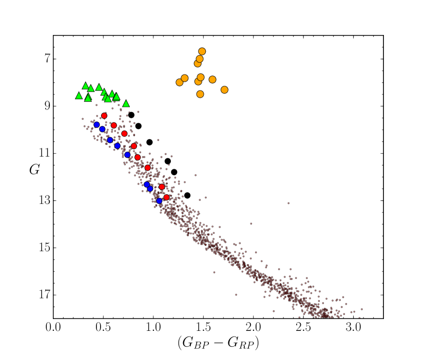
Figure 1: $G/(G_{\textrm{BP}}-G_{\textrm{RP}})$ diagram for Stock 2. Members from Cantat-Gaudin et al. (2018) are marked with light brown dots. Stars observed with CAOS in this work are represented with green triangles while those observed with HARPS-N appear as circles with different colours, as explained in the text.

2.1 Spectroscopy

We used HARPS-N (Cosentino et al., 2014) to observe the ten cluster giants on November 5 and 6, 2018. HARPS-N is an échelle spectrograph mounted at the 3.6-m TNG telescope at El Roque de los Muchachos Observatory (La Palma, Spain). It is fibre-fed from the Nasmyth B focus and covers the wavelength range from 3870 Å to 6910 Å providing a resolving power of $R=115\,000$. Later, still with the same equipment, we took spectra for 24 MS stars from 16 to 19 December 2018 and from 13 to 15 January 2019. The instrument’s pipeline was used to reduce these spectra.

We completed the TNG observations by collecting additional spectra for the 14 brightest stars of the upper MS around the TO point. Observations were carried out between 29 and 31 October 2020 with the Catania Astropysical Observatory Spectrograph (CAOS, Spanò et al., 2006; Leone et al., 2016). CAOS is an échelle spectrograph mounted on the 0.91-m telescope at M. G. Fracastoro station (Serra La Nave, Mt Etna (Italy)) which provides a resolution of $R=55\,000$. It is fibre-fed from the Cassegrain focus and covers, in 81 orders, the wavelength range from 3875 Å to 6910 Å. These spectra were reduced by employing the iraf packages following standard procedures. The log of the observations can be found in Table 1. This table displays the spectrograph used, the heliocentric Julian day at mid exposure (HJD), the exposure time ($t_{\textrm{exp}}$, which is the sum of all exposures of the same star), an estimate of the average signal-to-noise ratio per pixel achieved at 6500 Å ($S/N$) and the HD (or Tycho, or 2MASS) designation (Name).

Table 1: Observation log.

Star	Name	HJD	$t_{\textrm{exp}}$ (s)	$S/N^{a}$
HARPS-N
b1	HD 13967	58469.459	3000	111
b2	HD 13100	58469.420	3000	99
b3	TYC 3698-2381-1	58471.426	3600	98
b4	TYC 3699-1132-1	58472.519	7200	90
b5	TYC 3698-2224-1	58499.390	3800	82
b6	TYC 3698-483-1	58498.383	5400	58
b7	J02192173+5927303b	58470.375	9600	64
b8	J02204032+5923204b	58497.360	5400	30
r1	HD 12920	58499.473	1900	99
r2	TYC 3698-861-1	58469.498	3000	93
r3	TYC 3698-645-1	58471.506	3600	103
r4	TYC 3698-2739-1	58471.644	4800	67
r5	TYC 3697-479-1	58499.438	3800	78
r6	J02134650+5923569b	58498.450	5400	74
r7	TYC 3697-1499-1	58470.514	9600	61
r8	J02131100+5945191b	59178.387	6300	46
u1	HD 13699	58469.381	2400	147
u2	TYC 3698-1363-1	58469.537	3000	108
u3	TYC 3698-1420-1	58471.562	4800	95
u4	TYC 3698-1703-1	59131.598	3680	65
u5	J02134467+5933039b	59131.687	5520	73
u6	J02162746+5954309b	59131.748	4200	28
g1	HD 15498	58428.407	700	264
g2	HD 14346	58428.390	700	232
g3	HD 13437	58428.468	1400	346
g4	HD 13207	58428.450	1400	255
g5	HD 14403	58428.487	1400	282
g6	HD 12650	58428.423	1400	248
g7	HD 15665	58429.341	1400	242
g8	HD 14415	58428.505	1400	255
g9	HD 13655	58429.359	1400	211
g10	HD 13134	58429.378	1400	192
CAOS
to1	HD 14183	59152.498	2400	164
to2	HD 14161	59152.567	2700	153
to3	HD 12184	59152.529	2700	164
to4	HD 14025	59152.601	2700	89
to5	HD 13518	59153.510	2400	114
to6	HD 15240	59152.474	3000	70
to7	HD 13591	59153.541	2700	97
to8	HD 14946	59154.361	3000	69
to9	HD 14579	59153.615	2700	81
to10	HD 13909	59154.489	3000	153
to11	HD 13688	59153.576	2700	80
to12	HD 15315	59154.404	3000	115
to13	HD 13899	59154.526	3000	153
to14	HD 13606	59154.323	3000	45

Notes. ^a Signal-to-noise ratio per pixel at 6500 Å. ^b 2MASS designation.

2.2 Archival data

As mentioned above we started our investigation based on the work conducted by Cantat-Gaudin et al. (2018). From the analysis of $Gaia$-DR2 data they identified 1209 members for Stock 2. In the astrometric space, they located the cluster at ($\mu_{\alpha*}$, $\mu_{\delta}$, $\varpi$) = (15.966, $-$13.627, 2.641) $\pm$ (0.650, 0.591, 0.076), clearly standing out from the background (as seen in Fig. 2, which highlights the stars observed in this work). According to the spatial distribution of its members (Fig. 3) Cantat-Gaudin et al. (2018) placed the cluster centre at $\alpha$(2000) = 2h15m25.44s, $\delta$(2000) = +59^∘31^′19.2^′′, at a distance $\Delta(\alpha,\delta)$=(25.4^s,15.3^′) from the nominal value. Stock 2 is a dispersed cluster and half of its members ($r_{\textrm{50}}$) are found within a radius of 1.03^∘ around the centre, with the most distant ones positioned almost 4^∘ away. As a result, none of the photometric datasets existing in the literature cover its entire extension. For this reason, to complement our spectroscopy and the $Gaia$ data we resorted to all-sky photometric surveys. We used $JHK_{\textrm{S}}$ magnitudes from the 2MASS catalogue in the near infrared wavelength (Skrutskie et al., 2006) as well as $BVg^{\prime}r^{\prime}i^{\prime}$ optical bands from the APASS catalogue (Henden et al., 2016). In some cases, for the brightest stars for which the APASS photometry is not reliable we also made use of the values listed in the ASCC2.5 catalogue (Kharchenko & Roeser, 2009). The combination of all these data allowed us to analyse the CMDs of the cluster, as will be explained later in Sect. 5. All the astrometric and photometric data available for the stars observed in this work are summarised in Tables 9 and 10 in the appendix of the paper.

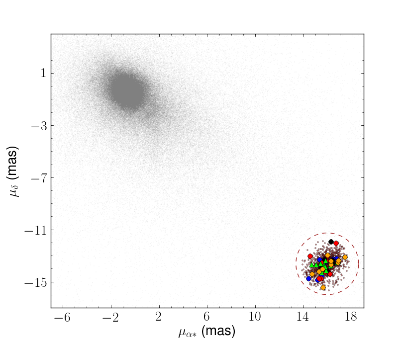
Figure 2: Proper-motion diagram in the field of Stock 2. The ellipse (brown dashed line) is centred in the average proper motions of the cluster and has semi axes of 4 times the sigmas of the $\mu_{\alpha*}$ and $\mu_{\delta}$ distributions of the cluster members according to Cantat-Gaudin et al. (2018). It represents the cluster extent in the astrometric space. Grey dots are field stars whereas the rest of the symbols are the same as those in Fig. 1.

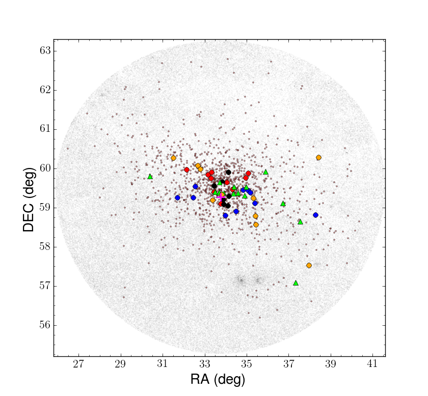
Figure 3: Sky region around Stock 2. Grey dots are the sources with $G$ $\leq$ 16 mag within a radius of 240 $\arcmin$ around the cluster nominal centre (magenta cross). Cluster members identified by Cantat-Gaudin et al. (2018) are represented by black points whereas the cluster centre derived from them is the white cross. Coloured circles and green triangles are the objects observed in this work (see Fig. 1) with the HARPS-N and CAOS spectrographs, respectively. The overdensities visible at RA$\sim 35^{\circ}$ and DEC$\sim 57^{\circ}$ correspond to $h$ & $\chi$ Per double cluster.

3 Spectral analysis

3.1 Radial velocity

We started the spectroscopic analysis by measuring the heliocentric radial velocity (RV) of the observed objects. For this purpose we cross-correlated our spectra against synthetic templates by employing the task fxcor contained in the iraf packages. When examining the cross-correlation function (CCF) we identified some multiple systems (SB2 or SB3) among the stars forming our sample namely, r4, u1 and u2. Therefore, in the upper sequence, we found only two binaries out of the six candidates, although the remaining four could be single-lined systems (SB1). Additionally, star u3 might also have a close companion since it shows a discrepant RUWE $Gaia$ parameter for a single source ($\approx$ 3.3). For the remaining single stars results are listed in the last column of Table 2. As can be seen, RVs show a large dispersion, with values ranging from $-$16.5 to $+$15.7 km s^-1. This is likely a consequence of the $v$ sin $i$ distribution. Indeed, while for slow rotators (e.g. giants and stars in the lower main-sequence) is possible determine precise RVs, for rapid rotators, instead, it is not. This is specially relevant for the hottest stars in our sample, located at the upper MS close to the TO point. These stars, with spectral types A, in addition to rotating rapidly, display far fewer features in their spectra, which broaden and reduce the intensity of the CCF peak. For this reason, to calculate the average RV for the cluster we only took the stars whose $v$ sin $i$¡50 km s^-1 into account. In this way, from 21 members, we derived an average value of $RV$=7.5$\pm$3.3 km s^-1. On the other hand, $Gaia$-DR2 (since the eDR3 does not provided new values) gives RV for 194 objects among the members listed in Cantat-Gaudin et al. (2018). The average value, after applying a 3$\sigma$-clipping filter to ignore outliers, is $RV_{\textrm{GDR2}}$=9.5$\pm$3.3 km s^-1 (which becomes 8.0 km s^-1 if, instead, the error-weighted mean is calculated). If we consider only the giants, the weighted average of our values is $RV$=7.9$\pm$1.4 km s^-1 (where we have assumed the weighted standard deviation as uncertainty), which is in close agreement with the above estimate.

3.2 Atmospheric parameters

To determine the stellar atmospheric parameters of our targets we used the rotfit code (Frasca et al., 2006) adapted to the SPA project workframe, as previously done (see e.g. Frasca et al., 2019; Casali et al., 2020). The code provides us not only with atmospheric parameters such as effective temperature ($T_{\textrm{eff}}$), surface gravity ($\log\,g$) and iron abundance ([Fe/H], as a proxy of the metallicity) but also with an estimate of the spectral type (SpT) and the projected rotational velocity ($v\,\sin\,i$). It should be noted that the last is a key parameter for the research we are conducting in this work. rotfit is based on a $\chi^{2}$ minimization of the difference between the target spectrum and a grid of templates. This difference is evaluated in 28 spectral segments of 100 Å each. Then, the final parameters are obtained by averaging the results of the individual regions, weighting them according to the $\chi^{2}$ and the information contained in each spectral segment. As template spectra we selected a collection of high-resolution spectra of real stars with well-known parameters taken with ELODIE ($R$ = 42 000). This grid of templates is the same as that used in the $Gaia$-ESO Survey by the Catania node (Smiljanic et al., 2014; Frasca et al., 2015). A more detailed description of our methodology can be found in Frasca et al. (2019).

For all the single stars, the results are displayed in Table 2. We obtained for this cluster an average solar metallicity of [Fe/H]=0.00$\pm$0.08, which was calculated as the weighted mean of the values for the spectra analyzed with rotfit. The error reflects the standard deviation of the individual values around the cluster mean.

rotfit is optimised to be used with FGK-type targets. Therefore, for hotter stars we used a different approach based on a grid of synthetic spectra computed as described in Sect. 3.3, for which we adopted an Opacity Distribution Function (ODF) computed for solar abundances. To determine $T_{\rm eff}$ and $\log g$ we used the wings and the cores of Balmer lines, while a region around the Mg ii$\lambda$4481 line has been used to derive the $v\sin i$. Due to the rapid stellar rotation, spectral lines are very broadened and shallow and then very difficult to measure, thus we have chosen to adopt [Fe/H] = 0.

Table 2: Stellar parameters derived for the single stars.

Star	$T_{\textrm{eff}}$ (K)	$\log\,g$	[Fe/H]	Sp T	$v\sin\,i$ (km s-1)	RV (km s-1)
b1	8500 $\pm$ 300	4.10 $\pm$ 0.20	0.00a	A1 Vb	140 $\pm$  15	13.44 $\pm$ 2.69
b2	8700 $\pm$ 200	4.00 $\pm$ 0.20	0.00a	A0 Vb	34.3 $\pm$ 4.7	9.37 $\pm$ 0.68
b3	7700 $\pm$ 300	4.07 $\pm$ 0.23	$-$0.19 $\pm$ 0.18	A7 V	280 $\pm$  30	15.65 $\pm$ 9.16
b4	7800 $\pm$ 300	4.09 $\pm$ 0.21	$-$0.21 $\pm$ 0.16	A7 V	120 $\pm$  15	8.03 $\pm$ 2.85
b5	7289 $\pm$ 252	4.05 $\pm$ 0.22	$-$0.16 $\pm$ 0.13	A9 IV	220 $\pm$  20	6.43 $\pm$ 8.04
b6	6132 $\pm$   91	4.11 $\pm$ 0.14	0.00 $\pm$ 0.10	F9 IV-V	21.9 $\pm$ 0.7	8.47 $\pm$ 0.23
b7	6092 $\pm$   73	4.20 $\pm$ 0.10	0.07 $\pm$ 0.10	F8 V	4.0 $\pm$ 1.0	$-$4.27 $\pm$ 0.10
b8	5841 $\pm$   86	4.42 $\pm$ 0.12	0.06 $\pm$ 0.08	G1 V	2.2 $\pm$ 1.7	5.74 $\pm$ 0.11
r1	8000 $\pm$ 250	3.90 $\pm$ 0.20	0.00a	A1 Vb	250 $\pm$ 30	$-$1.42 $\pm$ 6.35
r2	8300 $\pm$ 300	3.80 $\pm$ 0.30	0.00a	A1 Vb	230 $\pm$ 30	0.62 $\pm$ 3.09
r3	8800 $\pm$ 300	3.90 $\pm$ 0.20	0.00a	A0b	40 $\pm$   9	$-$3.69 $\pm$ 0.54
r5	7607 $\pm$ 279	4.11 $\pm$ 0.20	$-$0.09 $\pm$ 0.12	F0 III	135 $\pm$ 15	13.75 $\pm$ 5.81
r6	6851 $\pm$ 138	4.14 $\pm$ 0.11	$-$0.07 $\pm$ 0.09	F4 V	13.3 $\pm$1.0	9.65 $\pm$ 0.24
r7	6332 $\pm$ 163	4.04 $\pm$ 0.15	$-$0.06 $\pm$ 0.11	F7 IV	42 $\pm$   2	3.55 $\pm$ 0.83
r8	6086 $\pm$   73	4.20 $\pm$ 0.10	0.07 $\pm$ 0.10	F8 V	8.5 $\pm$0.8	9.02 $\pm$ 0.14
u3	7603 $\pm$ 299	4.01 $\pm$ 0.21	$-$0.13 $\pm$ 0.12	A8 V	53 $\pm$   6	9.26 $\pm$ 0.86
u4	8300 $\pm$ 300	4.10 $\pm$ 0.20	0.00a	B8 Vb	85 $\pm$ 10	$-$4.96 $\pm$ 0.29
u5	6449 $\pm$ 152	4.09 $\pm$ 0.16	$-$0.07 $\pm$ 0.11	F6 IV	44 $\pm$   1	3.38 $\pm$ 0.75
u6	6534 $\pm$ 131	4.11 $\pm$ 0.15	$-$0.05 $\pm$ 0.10	F8 V	41 $\pm$   1	2.27 $\pm$ 0.76
g1	4530 $\pm$   86	2.14 $\pm$ 0.10	0.01 $\pm$ 0.09	K1 III	1.6 $\pm$ 1.5	9.78 $\pm$ 0.12
g2	4760 $\pm$ 111	2.69 $\pm$ 0.14	0.02 $\pm$ 0.10	K0 III	7.6 $\pm$ 0.6	8.11 $\pm$ 0.13
g3	4937 $\pm$ 114	2.51 $\pm$ 0.35	0.04 $\pm$ 0.08	G8 III	6.1 $\pm$ 0.7	8.36 $\pm$ 0.13
g4	4977 $\pm$ 117	2.82 $\pm$ 0.18	0.04 $\pm$ 0.08	G8 III	1.7 $\pm$ 1.5	8.37 $\pm$ 0.11
g5	5061 $\pm$   56	2.99 $\pm$ 0.19	0.04 $\pm$ 0.07	G8 III	5.4 $\pm$ 1.2	9.20 $\pm$ 0.12
g6	5002 $\pm$ 110	2.96 $\pm$ 0.20	0.03 $\pm$ 0.07	G8 III	1.9 $\pm$ 1.6	7.10 $\pm$ 0.10
g7	5058 $\pm$   56	2.97 $\pm$ 0.20	0.03 $\pm$ 0.07	G8 III	2.7 $\pm$ 1.6	8.45 $\pm$ 0.11
g8	5065 $\pm$   56	3.00 $\pm$ 0.19	$-$0.03 $\pm$ 0.09	G8 III	5.2 $\pm$ 1.3	7.86 $\pm$ 0.11
g9	5062 $\pm$   56	3.00 $\pm$ 0.19	0.00 $\pm$ 0.09	G8 III	4.6 $\pm$ 1.4	4.38 $\pm$ 0.11
g10	5066 $\pm$   56	3.01 $\pm$ 0.19	$-$0.03 $\pm$ 0.09	G8 III	4.5 $\pm$ 0.9	8.66 $\pm$ 0.11
to1c	9300 $\pm$ 300	4.5 $\pm$ 0.2	0.00a	A1 Vb	80 $\pm$ 10	4.0 $\pm$ 11.7
to2	9100 $\pm$ 300	4.3 $\pm$ 0.2	0.00a	A2 IVb	60 $\pm$ 10	6.7 $\pm$   7.0
to3	9000 $\pm$ 300	4.1 $\pm$ 0.2	0.00a	A2 Vb	133 $\pm$ 10	2.8 $\pm$   7.7
to4	8300 $\pm$ 400	3.5 $\pm$ 0.2	0.00a	A1 Vb	199 $\pm$ 20	4.0 $\pm$ 10.0
to5	9000 $\pm$ 400	4.0 $\pm$ 0.2	0.00a	A1 Vb	108 $\pm$ 10	3.0 $\pm$   9.6
to6	9100 $\pm$ 300	4.3 $\pm$ 0.2	0.00a	A0 Vb	245 $\pm$ 25	9.3 $\pm$ 10.6
to7	8800 $\pm$ 400	4.5 $\pm$ 0.2	0.00a	A1 IVb	165 $\pm$ 15	10.3 $\pm$   1.7
to8	8800 $\pm$ 300	4.5 $\pm$ 0.2	0.00a	A1 Vb	94 $\pm$ 10	5.6 $\pm$   5.9
to9	8000 $\pm$ 400	3.5 $\pm$ 0.2	0.00a	A3 Vb	211 $\pm$ 20	0.4 $\pm$ 21.5
to10	9100 $\pm$ 300	4.4 $\pm$ 0.2	0.00a	A0 IVb	83 $\pm$ 10	7.4 $\pm$   4.8
to11	8800 $\pm$ 300	3.9 $\pm$ 0.2	0.00a	A0 IVb	11 $\pm$   5	8.3 $\pm$   0.1
to12	8800 $\pm$ 400	4.0 $\pm$ 0.2	0.00a	A0 Vb	228 $\pm$ 20	4.5 $\pm$   8.3
to13	8500 $\pm$ 400	3.6 $\pm$ 0.2	0.00a	A0 Vb	236 $\pm$ 25	8.2 $\pm$   8.3
to14	8800 $\pm$ 300	4.5 $\pm$ 0.2	0.00a	A0 Vb	144 $\pm$ 14	7.5 $\pm$   6.5

Notes. ^a Solar ODF adopted. ^b Spectral types adopted from SIMBAD. ^c Possible SB2 system.

3.3 Chemical abundances

In order to calculate the elemental abundances of our (single) targets we made use of the spectral synthesis technique (Catanzaro et al., 2011, 2013), as we already did within the SPA project previously (Frasca et al., 2019). As a starting point, we took the atmospheric parameters obtained with rotfit to compute 1D Local Thermodynamic Equilibrium (LTE) atmospheric models with the atlas9 code (Kurucz, 1993a, b). Then, we generated the corresponding synthetic spectra by using the radiative transfer code synthe (Kurucz & Avrett, 1981). As an optimization code we exploited ad hoc idl routines based on the amoeba minimization algorithm to find the best solution by minimizing the $\chi^{2}$ of the differences between the synthetic spectra and the observed ones. At this point, to check the validity of the input parameters we let them vary. We always found that the best solution is consistent with the rotfit values reported in Table 2, so we adopted them for the subsequent analysis. Once we checked the parameters we started to determine the abundances. We focused our analysis on 39 spectral regions of 50 Å each between 4400 and 6800 Å. In this way we derived the chemical abundances of 22 elements of atomic number up to 56, namely, C, O, Na, Mg, Al, Si, S, Ca, Sc, Ti, V, Cr, Mn, Fe, Co, Ni, Cu, Zn, Sr, Y, Zr, and Ba. For the hottest stars, those around the TO point observed with CAOS, it has been impossible to provide reliable abundances. These A-type stars, with effective temperatures above 8000 K, rotate with moderate/high velocities which prevent the analysis of the few spectral lines observed in their spectra. In fact, the bluest part of the spectra is not sufficiently well exposed even for classification purposes so we took the spectral types from the SIMBAD database.

Individual abundances for each star are listed, according to the standard notation $A($X$)=\log\,$[n(X)/n(H)] + 12, in Tables 11 and 12 for MS stars and giants, respectively. Additionally, the cluster mean abundances for each element, in terms of [X/H], are reported in Table 3. They have been calculated by means of the weighted average of each star, using the individual errors as weight. The abundances are expressed referring to the solar value that we obtained by applying the same procedure to a HARPS-N spectrum of Ganymede (see table 5 in Frasca et al., 2019).

For what concerns iron, with the exception of the hottest and fast rotating stars for which we can not measure its abundance, we found an average [Fe/H]=$-$0.13$\pm$0.08. This value is slightly lower than that derived by using rotfit but still compatible within the errors. In any case, for clarity’s sake, hereinafter we adopted the weighted mean of both values (obtained from rotfit and synthe, respectively) as the iron content of the cluster, i.e. [Fe/H]=$-$0.07$\pm$0.06.

We find that abundances derived from giants and dwarfs are compatible within the errors for all the elements except for Ba and Sr, which are clearly overabundant in giants (0.48 and 0.38 dex, respectively), and Co, which is only marginally overabundant. For the remaining elements significant discrepancies are not seen. Only for Na, V, and Cu differences are $\geq$ 0.15 dex, but still consistent with each other. Stock 2 shows solar weighted-mean ratios for $\alpha$-elements ([$\alpha$/Fe]=0.04$\pm$0.05, without including the O) and iron-group elements ([X/Fe]=0.03$\pm$0.03) while for the heaviest elements, without taking into account Sr and Ba, the cluster exhibits a supersolar ratio ([$s$/Fe]=0.17$\pm$0.04).

Table 3: Average chemical abundances ([X/H]) for Stock 2 obtained with synthe.

Element	Total	MS stars	Giants
C	$-$0.08 $\pm$ 0.05	$-$0.08 $\pm$ 0.05	…
O	$-$0.20 $\pm$ 0.03	$-$0.20 $\pm$ 0.03	…
Na	$+$0.14 $\pm$ 0.14	$+$0.08 $\pm$ 0.14	$+$0.23 $\pm$ 0.14
Mg	$-$0.20 $\pm$ 0.10	$-$0.25 $\pm$ 0.10	$-$0.15 $\pm$ 0.10
Al	$-$0.13 $\pm$ 0.15	$-$0.18 $\pm$ 0.16	$-$0.12 $\pm$ 0.15
Si	$+$0.05 $\pm$ 0.08	$+$0.03 $\pm$ 0.09	$+$0.07 $\pm$ 0.09
S	$+$0.05 $\pm$ 0.10	$+$0.00 $\pm$ 0.11	$+$0.14 $\pm$ 0.11
Ca	$-$0.04 $\pm$ 0.09	$-$0.02 $\pm$ 0.09	$-$0.09 $\pm$ 0.10
Sc	$+$0.01 $\pm$ 0.13	$+$0.00 $\pm$ 0.13	$+$0.03 $\pm$ 0.14
Ti	$-$0.06 $\pm$ 0.12	$-$0.08 $\pm$ 0.12	$-$0.01 $\pm$ 0.13
V	$+$0.06 $\pm$ 0.10	$+$0.14 $\pm$ 0.11	$-$0.03 $\pm$ 0.11
Cr	$+$0.02 $\pm$ 0.15	$-$0.04 $\pm$ 0.15	$+$0.09 $\pm$ 0.15
Mn	$-$0.07 $\pm$ 0.15	$-$0.09 $\pm$ 0.16	$-$0.05 $\pm$ 0.15
Fe	$-$0.13 $\pm$ 0.08	$-$0.15 $\pm$ 0.09	$-$0.10 $\pm$ 0.09
Co	$+$0.01 $\pm$ 0.05	$+$0.08 $\pm$ 0.06	$-$0.09 $\pm$ 0.06
Ni	$-$0.04 $\pm$ 0.10	$-$0.01 $\pm$ 0.10	$-$0.07 $\pm$ 0.11
Cu	$-$0.22 $\pm$ 0.10	$-$0.16 $\pm$ 0.10	$-$0.31 $\pm$ 0.11
Zn	$-$0.16 $\pm$ 0.09	$-$0.20 $\pm$ 0.10	$-$0.13 $\pm$ 0.09
Sr	$+$0.09 $\pm$ 0.15	$-$0.02 $\pm$ 0.15	$+$0.46 $\pm$ 0.16
Y	$+$0.11 $\pm$ 0.04	$+$0.12 $\pm$ 0.04	$+$0.06 $\pm$ 0.06
Zr	$+$0.00 $\pm$ 0.14	$+$0.01 $\pm$ 0.15	$-$0.01 $\pm$ 0.14
Ba	$-$0.11 $\pm$ 0.09	$-$0.20 $\pm$ 0.09	$+$0.18 $\pm$ 0.09

4 Reddening and SED fitting

With the aim of determining the interstellar extinction ($A_{V}$) of our sources, as well as the luminosity ($L$), we resorted to the spectral energy distribution (SED) fitting method. From optical and NIR photometric data publicly available we built the corresponding SED, which was fitted with BT-Settl synthetic spectra (Allard, 2014). For each target, we assumed its $Gaia$-eDR3 parallax as well as the atmospheric parameters ($T_{\textrm{eff}}$ and $\log\,g$) obtained in Sect. 3.2, leaving the stellar radius ($R$) and $A_{V}$ as free parameters. These parameters were then obtained by $\chi^{2}$ minimization and the stellar luminosity was calculated as $L$=4 $\pi$ $R^{2}$ $\sigma$ $T_{\textrm{eff}}^{4}$. An example of this fitting is shown in Fig. 4. The errors on $A_{V}$ and $R$ are found by the minimization procedure considering the 1-$\sigma$ confidence level of the $\chi^{2}$ map, but we have also taken the error on $T_{\rm eff}$ into account .

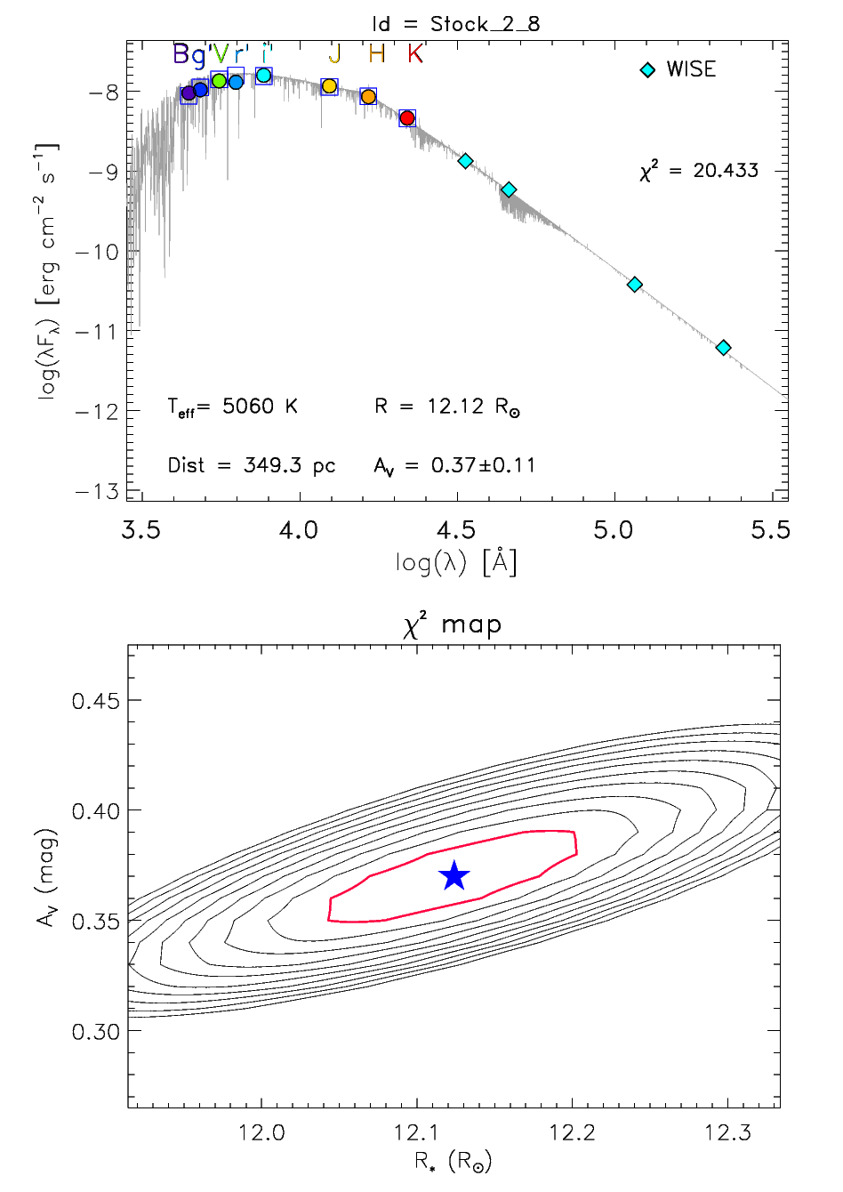
Figure 4: Top: Example of a SED fitting (star g8). Bottom: $\chi^{2}$-contour map of the fitting. The red contour corresponds to the 1-$\sigma$ confidence level.

The $A_{V}$ values thus obtained are reported in Table 4. In total, we provide results for 42 stars, whose $A_{V}$ range from 0.37 to 1.93 mag, with an average of $A_{V}$=0.84$\pm$0.34, where the error is the standard deviation. This extinction corresponds to $E(B-V)$=0.27$\pm$0.11 when assuming a standard reddening law with $R_{V}$=3.1. The high dispersion confirms the existence of a noticeable differential reddening across the observed field, as described in previous studies (Krzeminski & Serkowski, 1967; Spagna et al., 2009). Indeed, our value is compatible within the errors with that mostly accepted for the cluster, $E(B-V)\approx$0.35 (Ye et al., 2021).

Alternatively, we evaluated the reddening from the colour excess definition, that is, by comparing observed and intrinsic colours for each star. For this purpose we used the 2MASS photometric data shown in Table 10, since they are more suitable than the optical ones as they are less affected by the extinction. The intrinsic colours were adopted from the spectral types (Table 2) according to the calibrations of Straižys & Lazauskaitė (2009). In this way, from 43 stars, we obtained an average cluster reddening of $E(B-V)$=0.26$\pm$0.11, which shows an excellent agreement with the value derived from the SED fitting. This agreement is especially remarkable considering that photometric calibrations do not take the effect of the rotational velocity on the colour into account.

Table 4: Results of the SED fitting.

Star	$A_{V}$ (mag)	$R$ (R☉)	$L$ (L☉)
b1	0.65 $\pm$ 0.17	2.23 $\pm$ 0.03	23.4 $\pm$ 3.2
b2	0.77 $\pm$ 0.08	2.12 $\pm$ 0.04	23.2 $\pm$ 2.1
b3	0.42 $\pm$ 0.22	1.85 $\pm$ 0.02	10.9 $\pm$ 1.7
b4	0.73 $\pm$ 0.24	1.80 $\pm$ 0.03	10.7 $\pm$ 1.6
b5	0.77 $\pm$ 0.25	1.64 $\pm$ 0.03	6.8 $\pm$ 0.9
b6	0.45 $\pm$ 0.10	1.15 $\pm$ 0.02	1.7 $\pm$ 0.1
b7	0.47 $\pm$ 0.09	1.08 $\pm$ 0.02	1.4 $\pm$ 0.1
b8	0.46 $\pm$ 0.11	0.98 $\pm$ 0.02	1.0 $\pm$ 0.1
r1	0.53 $\pm$ 0.25	2.84 $\pm$ 0.05	29.7 $\pm$ 4.4
r2	0.85 $\pm$ 0.19	2.45 $\pm$ 0.03	25.7 $\pm$ 3.7
r3	1.28 $\pm$ 0.09	2.37 $\pm$ 0.03	30.2 $\pm$ 4.1
r5	1.06 $\pm$ 0.22	1.68 $\pm$ 0.03	8.5 $\pm$ 1.2
r6	0.94 $\pm$ 0.17	1.55 $\pm$ 0.02	4.8 $\pm$ 0.3
r7	0.86 $\pm$ 0.16	1.21 $\pm$ 0.02	2.1 $\pm$ 0.2
r8	0.82 $\pm$ 0.07	1.06 $\pm$ 0.01	1.4 $\pm$ 0.1
u3	1.29 $\pm$ 0.23	2.55 $\pm$ 0.04	19.6 $\pm$ 3.0
u4	1.93 $\pm$ 0.20	1.91 $\pm$ 0.03	15.5 $\pm$ 2.2
u5	1.23 $\pm$ 0.16	1.77 $\pm$ 0.02	4.9 $\pm$ 0.4
u6	1.51 $\pm$ 0.10	1.23 $\pm$ 0.02	2.5 $\pm$ 0.2
g1	0.40 $\pm$ 0.30	29.84 $\pm$ 1.55	337.6 $\pm$ 31.1
g2	0.58 $\pm$ 0.31	24.85 $\pm$ 0.48	285.4 $\pm$ 27.2
g3	0.66 $\pm$ 0.27	21.27 $\pm$ 0.30	242.6 $\pm$ 22.5
g4	0.82 $\pm$ 0.26	17.36 $\pm$ 0.23	166.9 $\pm$ 15.7
g5	0.53 $\pm$ 0.13	14.99 $\pm$ 0.20	132.7 $\pm$ 5.9
g6	1.15 $\pm$ 0.25	18.30 $\pm$ 0.21	188.5 $\pm$ 16.6
g7	0.85 $\pm$ 0.12	15.62 $\pm$ 0.24	144.0 $\pm$ 6.7
g8	0.37 $\pm$ 0.11	12.12 $\pm$ 0.17	86.8 $\pm$ 3.9
g9	1.43 $\pm$ 0.08	15.78 $\pm$ 0.26	147.0 $\pm$ 6.8
g10	0.90 $\pm$ 0.08	12.33 $\pm$ 0.13	90.5 $\pm$ 3.9
to2	0.78 $\pm$ 0.14	4.58 $\pm$ 0.05	129.3 $\pm$ 16.9
to3	0.59 $\pm$ 0.15	4.38 $\pm$ 0.08	113.3 $\pm$ 15.1
to4	0.65 $\pm$ 0.34	4.50 $\pm$ 0.09	86.4 $\pm$ 16.7
to5	1.00 $\pm$ 0.20	4.42 $\pm$ 0.09	115.2 $\pm$ 20.5
to6	0.37 $\pm$ 0.17	3.11 $\pm$ 0.07	59.8 $\pm$ 7.9
to7	1.04 $\pm$ 0.22	4.39 $\pm$ 0.06	104.0 $\pm$ 18.9
to8	0.48 $\pm$ 0.17	3.54 $\pm$ 0.05	67.6 $\pm$ 9.1
to9	0.77 $\pm$ 0.36	4.59 $\pm$ 0.08	77.8 $\pm$ 15.5
to10	0.90 $\pm$ 0.13	3.96 $\pm$ 0.07	96.9 $\pm$ 12.7
to11	1.06 $\pm$ 0.19	4.22 $\pm$ 0.12	95.9 $\pm$ 13.3
to12	0.61 $\pm$ 0.24	3.62 $\pm$ 0.10	70.7 $\pm$ 12.9
to13	0.93 $\pm$ 0.27	4.13 $\pm$ 0.11	80.2 $\pm$ 15.1
to14	1.23 $\pm$ 0.22	4.03 $\pm$ 0.15	87.8 $\pm$ 12.4

5 Colour-magnitude diagrams

With the aim of investigating the age of the cluster we combined archival photometry with the spectroscopy obtained in this work. We made use of the most widespread procedure, the so-called isochrone-fitting method. It consists of finding the age-dependent model, isochrone, that best reproduces the cluster evolutionary snapshot reflected in its CMD. In a first step, it was necessary to construct the CMD. We did it in three different photometric systems (optical, 2MASS and $Gaia$-eDR3), highlighting our targets in Fig. 5, according to the criterium described in Sect. 2. We took advantage of the reddening previously obtained ($E(B-V)$=0.27, Sect. 4) to draw the following diagrams: $M_{V}$/$(B-V)_{0}$, $M_{K_{\textrm{S}}}$/$(J-K_{\textrm{S}})_{0}$ and $G$/$(G_{BP}-G_{RP})$. Individual distances, derived from the inversion of their parallaxes, were also taken into account. Individual zero-point offset corrections, with an average value around $-$33 $\mu$as, were applied to the published $Gaia$-eDR3 parallaxes following the recommendations outlined by Lindegren et al. (2021). Then, in a second step, we drew PARSEC isochrones (Bressan et al., 2012) for different ages computed at the metallicity found in this work ([Fe/H]=$-$0.07, see Sect. 3.3). With the intention of ensuring the reliability of the fit, we selected, among the list of members identified by Cantat-Gaudin et al. (2018), only those with a membership probability sufficiently high (i.e. $P\geq$0.7). Additionally, on this sample we imposed a quality cutoff, taking only the objects whose error on parallax is below 0.1 mas, i. e. with an uncertainty less than 5$\%$. In total we considered 1016 cluster members with $Gaia$-eDR3 photometry. We did a cross-match of our member list with the APASS (Henden et al., 2016) and 2MASS (Skrutskie et al., 2006) catalogues and then we selected only the stars with good-quality photometry. In the first case this meant stars with errors on both $V$ and $(B-V)$ ¡ 0.1 mag, while in the second case, just the stars without any ‘$U$’ photometric flag assigned. In total 409 and 955 objects were retrieved, respectively. The resulting diagrams are displayed in Fig. 5.

When building the first CMD ($M_{V}$/$(B-V)_{0}$) we immediately realised the wrong position of the brightest stars, among which were many of our targets. For these stars the APASS photometry provide errors above one magnitude or even not quantified. With this purpose we resorted to the ASCC2.5 catalogue (Kharchenko & Roeser, 2009) from which we took $V$ and $(B-V)$ for stars brighter than $V$=10, after scaling both photometric datasets. Then, we dereddened the CMD (left panel of Fig. 5) by applying individual corrections to the stars for which we have spectra and the average value to the rest of stars. Finally, we plotted the isochrone that best reproduces the CMD based on a visual inspection, from which we obtained for the cluster a log $\tau$=8.65$\pm$0.15 (equivalent to an age of 450$\pm$150 Ma). In this case, the error reflects the interval of isochrones that gives a good fit. With this age the MSTO stellar mass is $\approx$2.8 M_☉. In general, stars occupy positions close to the isochrone and only the TO stars seem to be slightly away from it.

Regarding the 2MASS CMD, the fit is quite good and all stars match the isochrone rather well, with the exception of the star g1. It is the brightest in the cluster and shows a position away from the the rest of the giants. As it is so bright, it is close to saturate and its photometry, flagged in the catalogue as ‘$EDD$’, has errors in each band of around 0.2 mag. Therefore, its anomalous $(J-K)$ colour could simply be an instrumental effect. Some residual dispersion is still observed for the MS stars, although the correction for reddening has been applied; moreover in the NIR the reddening is lower than at optical wavelengths and should play a minor role on the CMD. After the reddening correction, no clear eMSTO/split MS is apparent in the CMD. Giants show a dispersion in magnitude greater than it would be expected from their atmospheric parameters, which are very similar to each other.

In the last diagram, the $Gaia$-eDR3 CMD, since the dereddening of the $Gaia$ photometry is not a trivial task, the isochrone (and not the stars as in the previous CMDs) was reddened using the average extinction obtained in Sect. 4. A distance modulus of 7.87, which corresponds to the distance derived by Cantat-Gaudin et al. (2018), was applied. The fit is also good and stars lie along the isochrone.

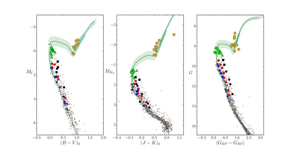
Figure 5: Colour-magnitudes diagrams for Stock 2 in three different photometric systems: Left: $M_{V}$/$(B-V)_{0}$, photometric data from the APASS catalogue; Centre: $M_{K_{\textrm{S}}}$/$(J-K_{\textrm{S}})_{0}$ (2MASS) and Right: $G$/$(G_{BP}-G_{RP})$ ($Gaia$-eDR3). Colours and symbols are the same as those in Fig. 1. The green line and the shaded area are the best-fitting isochrone within the uncertainties (log $\tau$=8.65$\pm$0.15).

6 Discussion

One of the objectives of this research was to determine the age of the cluster. Now, based on $Gaia$-eDR3 individual parallaxes for the cluster members and the extinction derived from the SED fitting we were able to build suitable CMDs, in which the cluster age was obtained via the isochrone-fitting method. By analysing the dereddened 2MASS CMD, which is less affected by the interstellar dust than the ones at optical wavelengths used in past works, we can asses that Stock 2 is a moderately young open cluster of 450$\pm$150 Ma. Therefore, it is somewhat younger than the Hyades and clearly older than the Pleiades. This confirms the results of Spagna et al. (2009) and Sciortino et al. (2000) over older studies (e.g. Krzeminski & Serkowski, 1967).

The RVs obtained by us are, in general, compatible within the errors with those found in the literature, as displayed in Table 5 for stars in common with Mermilliod et al. (2008), who measured RVs for red giants in open clusters, and Reddy & Lambert (2019). Although Mermilliod et al. (2008) claimed binarity for g3 and g9, we have not seen any feature in their spectra that might confirm it, as also Reddy & Lambert (2019) concluded. However, given the discrepancies for the latter, perharps it might be a long-period variable. Figure 6 shows the stars for which we have derived their RV compared, when possible, to the values obtained by $Gaia$-DR2. We remark the excellent agreement for the slow rotators, especially in the case of giant stars. For fast rotators, instead, as we already noted, our errors are very large and results are not very reliable; for most of them $Gaia$-DR2 does not provide any RV.

Table 5: Comparison of the RV (km s^-1) derived in this work and in the literature.

Star	Me08	$Gaia$-DR2	Reddy19	This work
g3	9.6 $\pm$ 1.3	8.5 $\pm$ 0.2	8.8 $\pm$ 0.1	8.4 $\pm$ 0.1
g4	8.1 $\pm$ 0.4	8.4 $\pm$ 0.1	8.6 $\pm$ 0.1	8.4 $\pm$ 0.1
g9	7.8 $\pm$ 0.8	4.7 $\pm$ 0.2	4.4 $\pm$ 0.1	4.4 $\pm$ 0.1

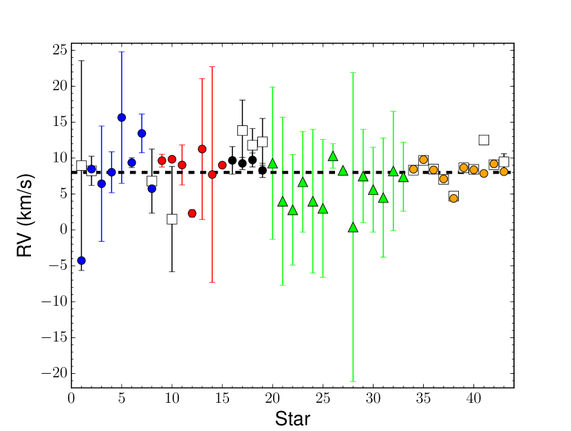
Figure 6: Comparison of the RVs obtained in this work (symbols and colours as in previous figures) with those of $Gaia$-DR2 (open squares). The dashed line shows the cluster average value, $RV$=8.0 km s^-1.

Regarding the atmospheric parameters, as already mentioned, Reddy & Lambert (2019) conducted the only spectroscopy-based paper devoted to Stock 2. Their study is based on high-resolution spectra ($R$=60 000) of three of the cluster giants. These stars, which have also been observed by us, are g3 (numbered as 43 in their work), g4 (1011) and g9 (1082). Our temperatures and metallicities are slightly larger but still in agreement with their values, within the errors. Instead, gravities are only marginally compatible. Both datasets are compared in Table 6. These discrepancies probably can be explained because of the different methodology followed. In this work we employed spectral fitting while their approach was based on the equivalent width (EW) analysis.

Table 6: Comparison of the atmospheric parameters derived in this work with those of the literature.

Star	This work			Reddy & Lambert (2019)
	$T_{\textrm{eff}}$ (K)	$\log\,g$	[Fe/H]	$T_{\textrm{eff}}$ (K)	$\log\,g$	[Fe/H]
g3	4937 $\pm$ 114	2.51 $\pm$ 0.35	0.04 $\pm$ 0.08	4925 $\pm$ 50	2.0 $\pm$ 0.1	$-$0.07 $\pm$ 0.03
g4	4977 $\pm$ 117	2.82 $\pm$ 0.35	0.04 $\pm$ 0.08	4900 $\pm$ 50	2.3 $\pm$ 0.1	$-$0.05 $\pm$ 0.04
g9	5062 $\pm$ 56	2.98 $\pm$ 0.18	0.00 $\pm$ 0.09	5050 $\pm$ 50	2.6 $\pm$ 0.1	$-$0.06 $\pm$ 0.03

With the aim of checking the consistency of our results, we plot the Kiel and HR diagrams in Fig. 7. The former is a reddening-free diagnostic whereas in the latter, extinction has been taken into account when calculating the luminosity. The location of the stars in the HR diagram is better than in the Kiel diagram, where gravities lie away with respect to those of the isochrone around 0.2 dex, as already came out in the comparison with results from Reddy & Lambert (2019). Additionally, TO stars show a large dispersion in this diagram. This is very likely a consequence of the poor accuracy of the gravity determinations for these A-type stars, which have a moderate or fast rotation. On the contrary, in the HR diagram these stars are placed more closely clustered around the TO point, as it is expected. The fit is also better for MS stars and especially good for giants, which fall on the isochrone.

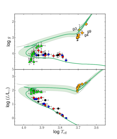
Figure 7: Kiel and HR diagrams for Stock 2. Symbols and colours are the same as those in Fig. 5.

6.1 Chromospheric emission and lithium abundance

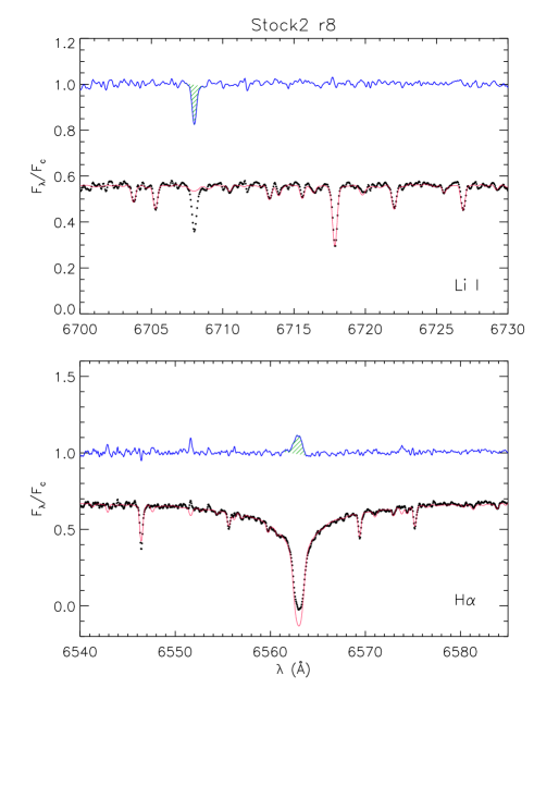
Figure 8: Subtraction of the non-active, lithium-poor template (red line) from the spectrum of Stock2 r8 (black dots), which reveals the chromospheric emission in the H$\alpha$ core (blue line in the bottom panel) and emphasizes the Li i $\lambda$6708 Å absorption line, removing the nearby blended lines (top panel). The green hatched areas represent the excess H$\alpha$ emission (bottom panel) and Li i absorption (top panel) that were integrated to obtain $EW_{\rm H\alpha}^{em}$ and $EW_{\rm Li}$, respectively.

For stars cooler than about 6500 K and with an age from a few ten to a few hundred Ma, the level of magnetic activity (e.g. the emission in the cores of lines formed in the chromosphere) and the atmospheric lithium abundance can be used to estimate the age (see, e.g., Jeffries, 2014; Frasca et al., 2018, and references therein). The best diagnostics of chromospheric emission in the wavelength range covered by HARPS-N are Ca ii H&K and Balmer H$\alpha$ lines. However, the S/N ratio at 3900 Å is very low, so that we can only use the H$\alpha$ for this purpose. The templates produced by rotfit with rotationally broadened spectra of non-active, lithium-poor stars were subtracted from the observed spectra of the targets to measure the excess emission in the core of the H$\alpha$ line ($EW_{\rm H\alpha}^{em}$) and the equivalent width of the Li i $\lambda$6708 Å absorption line ($EW_{\rm Li}$), removing the blends with nearby lines.

Table 7: H$\alpha$, Li i$\lambda$6708 Å equivalent widths and lithium abundance for the targets cooler than 7000 K.

Star	$T_{\rm eff}$	$EW_{\rm H\alpha}^{em}$	err	$EW_{\rm Li}$	err	$A$(Li)
	(K)	(mÅ)		(mÅ)		(dex)
b6	6132	143	24	63	6	$2.68^{+0.10}_{-0.10}$
b7	6092	$\dots$	$\dots$	¡3	$\dots$	$<$1.27
b8	5841	72	31	145	12	$2.93^{+0.11}_{-0.10}$
r6	6851	$\dots$	$\dots$	54	5	$3.03^{+0.12}_{-0.13}$
r7	6332	50	15	9	6	$1.91^{+0.31}_{-0.56}$
r8	6086	110	17	89	10	$2.88^{+0.10}_{-0.11}$
u5	6449	38	13	32	6	$2.55^{+0.18}_{-0.20}$
u6	6534	93	37	15	10	$2.23^{+0.32}_{-0.55}$

Figure 8 shows an example of the subtraction procedure used to measure the equivalent width of H$\alpha$ and lithium lines, $EW_{\rm H\alpha}^{em}$ and $EW_{\rm Li}$. These quantities were measured on the subtracted spectra by integrating the residual emission and absorption profiles, as shown by the green dashed areas in Fig. 8, and are reported in Table 7.

A simple method to get an estimate of a star’s age independent of that derived from isochrones is to compare its position in a diagram that plots lithium abundance, $A$(Li), versus $T_{\rm eff}$ with the upper envelopes of clusters with a known age. We calculated the lithium abundance, $A$(Li), from our values of $T_{\rm eff}$, $\log g$, and $EW_{\rm Li}$ by interpolating the curves of growth of Lind et al. (2009), which span the $T_{\rm eff}$ range 4000–8000 K and $\log g$ from 1.0 to 5.0 and include non-LTE corrections. In Fig. 9 we show the lithium abundance as a function of $T_{\rm eff}$ along with the upper envelopes of the distributions of some young open clusters shown by Sestito & Randich (2005). Apart from the large errors of $A$(Li), which take into account both the $T_{\rm eff}$ and $EW_{\rm Li}$ errors, Fig. 9 shows that all the targets are located close or below the Hyades upper envelope, compatible with an age $\approx$ 600 Ma. The only exception is the coldest target, b8, which lies between the upper envelopes of the Pleiades ($\approx$ 100 Ma) and NGC 6475 ($\approx$ 300 Ma), which suggests an age $\lesssim 300$ Ma for this star. However, for stars with $T_{\rm eff}$¿6000 K the upper envelopes are very close to each other, which hampers the estimation of the cluster’s age with this method. Lithium abundances for colder stars, where the envelopes separate more, would be extremely useful in clarifying this point. Unfortunately, the combination of very high resolution and telescope size did not permit to reach the low main sequence. Hopefully, large samples of fainter stars will be acquired, e.g. by the survey WEAVE (Dalton et al., 2020) due to start soon at the 4.2-m William Herschel Telescope.

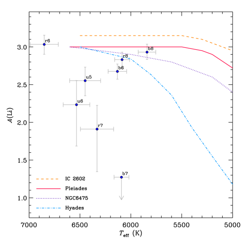
Figure 9: Lithium abundance as a function of $T_{\rm eff}$. The upper envelopes of $A$(Li) for IC 2602 ($age\approx$ 30 Ma), Pleiades ($\approx$ 100 Ma), NGC 6475 ($\approx$ 300 Ma), and Hyades ($\approx$ 600 Ma) clusters adapted from Sestito & Randich (2005) are overplotted.

6.2 Galactic metallicity gradient

Open clusters are good tracers of the radial metallicity distribution of the Galaxy (i.e. the so-called Galactic gradient). To see how the metallicity derived for Stock 2 in this work compares with the general gradient, we collected a sample of homogeneously analysed clusters from the $Gaia$-ESO iDR5 and iDR6 (Baratella et al., 2020; Magrini et al., 2021) and the APOGEE DR16 surveys (Donor et al., 2020). From the latter we only took clusters with data derived from two or more stars and closer than 15 kpc. In addition, open clusters from Alonso-Santiago et al. (2017, 2018, 2019, 2020) are also added to the sample along with those previously investigated within the SPA project (Frasca et al., 2019; D’Orazi et al., 2020; Casali et al., 2020; Zhang et al., 2021). In total, for this comparison we gathered more than a hundred clusters, ten of which are in common among different datasets. Figure 10 shows the location of Stock 2 in the Galactic gradient. Galactocentric distances have been taken from Cantat-Gaudin et al. (2018), which obtained their distances from the $Gaia$-DR2 parallaxes, taking as a reference for the solar value $R_{\sun}$=8.34 kpc. The metallicity, in terms of iron abundance, was referenced to $A$(Fe)=7.45 dex (Grevesse et al., 2007). The metallicity found in this work is compatible with that expected for its position.

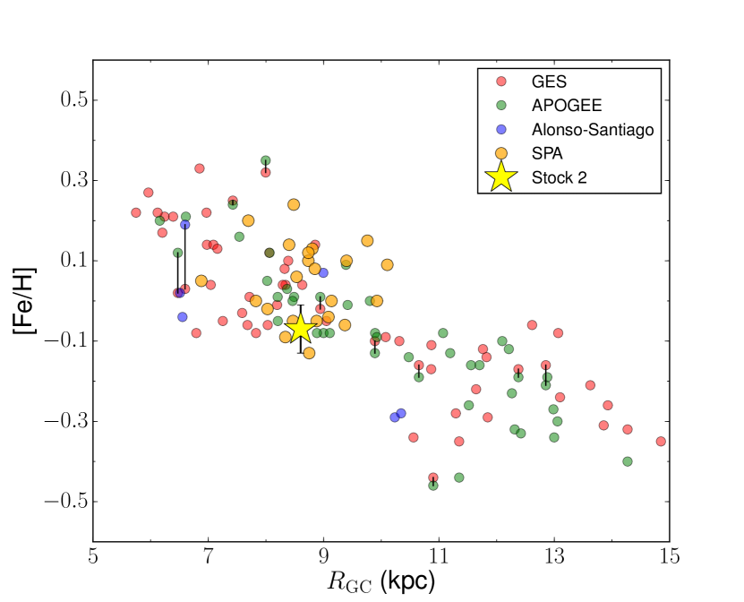
Figure 10: Radial metallicity gradient from open clusters studied in the framework of the $Gaia$-ESO (Baratella et al., 2020; Magrini et al., 2021, red circles) and APOGEE (Donor et al., 2020, green circles) surveys. Other similar clusters analysed by Alonso-Santiago et al. (2017, 2018, 2019, 2020, blue circles) are also added along to those previously investigated in the SPA project (Frasca et al., 2019; D’Orazi et al., 2020; Casali et al., 2020; Zhang et al., 2021, orange circles). Black lines link results for the same cluster provided by different authors. The star-symbol represents Stock 2.

6.3 Chemical composition and Galactic trends

Regarding the abundances, we compared our results (separately for MS stars and giants) to those of Reddy & Lambert (2019), with which we have 17 chemical elements in common. For the comparison, the values from Reddy & Lambert (2019) have been scaled to our solar references. In Fig. 11 the differences of the abundance ratios ([X/H]), this work minus literature, are displayed. As expected, differences are smaller for giants (on average, $\Delta$[X/H]=0.07 dex) than for MS stars (0.12 dex). With the only exception of Y, the chemical composition of all the giants is fully compatible with that obtained by Reddy & Lambert (2019). On the other hand, for MS stars, abundances for Na, V, Co, Zn, Y and Ba are somewhat different.

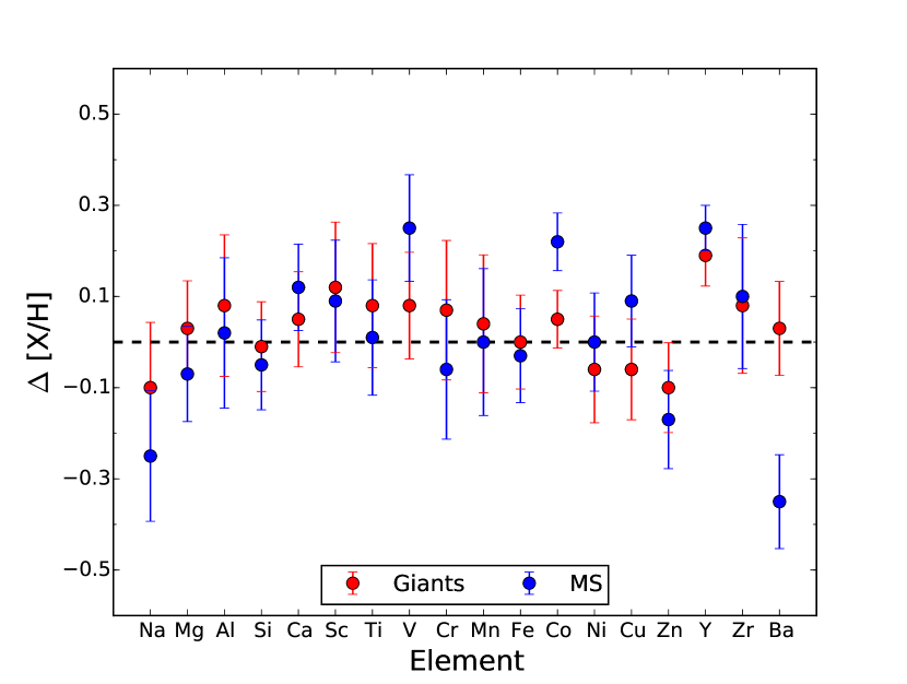
Figure 11: Differences between our mean abundances, for giants and MS stars, and those by Reddy & Lambert (2019). The error bars are the quadratic sum of the uncertainties reported in both studies for each element.

Finally, as we have done above in relation to the metallicity gradient, we contrast the abundances obtained in this work with those of the comparison clusters selected before. We completed the sample by adding the $Gaia$-ESO DR4 abundances (Magrini et al., 2017, 2018) for the clusters in common with Magrini et al. (2021). In total, we have in common with them up to 18 chemical elements, out of which the ratios [X/Fe] versus [Fe/H] are displayed in Fig. 12 for 16 chemical elements. The remaining two are O and Ba but since for these elements, the measure of the abundances is conditioned by the evolutionary state of the stars (see Sect. 3.3), we discarded them from the comparison. In general, Stock 2 shows a chemical composition compatible with that of the Galactic thin disc, as supported by the agreement with the observed chemical trends traced by more than a hundred open clusters. Only the abundance of Cu is sligthtly below these trends, but it is still compatible with them.

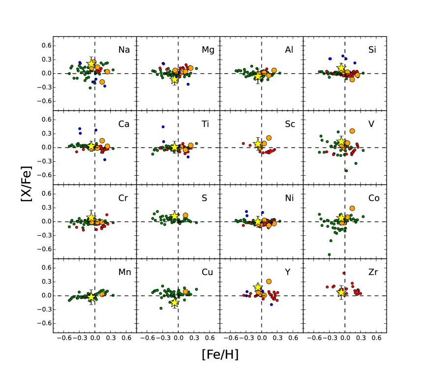
Figure 12: Abundance ratios [X/Fe] vs. [Fe/H]. Symbols and colours are the same as in Fig. 10. The dashed lines indicate the solar value.

6.4 Rotational velocity, reddening and eMSTO

We investigated the relationship between $v$ sin $i$ and the eMSTO phenomenon. As mentioned in Sect. 2, we selected our targets following in the CMD of Fig. 1 three different sequences along the MS: blue, red and the upper envelope. Among all the stars observed in this work around 40$\%$ rotate rapidly (with $v$ sin $i$ ¿ 100 km s^-1). As can be seen in Table 2, in general, the fastest rotators are found among the brightest stars in each sequence but also a large scatter of velocities is detected. According to the literature (Dupree et al., 2017; Marino et al., 2018b; Sun et al., 2019) the bMS should be populated by stars that rotate slower than those in the rMS. However, this is not what we observe in this work. Significant differences are not found in the mean $v$ sin $i$ of both sequences. In addition, for those single stars in the group in which we expected to find binaries (the upper envelope sequence), their $v$ sin $i$ are smaller than in the two other series, despite being redder even than the rMS stars (see Table 8).

Table 8: Mean projected rotational velocities (km s^-1) and reddening along MS stars. N is the number of stars in each category.

MS sequence (N)	$v$ sin $i$	$A_{V}$
	(km s-1)	(mag)
bMS (8)	103 $\pm$ 106	0.59 $\pm$ 0.15
rMS (7)	100 $\pm$   98	0.91 $\pm$ 0.23
uMS (4)	57 $\pm$   22	1.49 $\pm$ 0.32

To interpret this phenonomenon the contribution of the reddening should not be ignored. The cluster average value obtained in this work is compatible within the errors with that expected for its position according to the extinction maps obtained by Lallement et al. (2019). However, as noted above, its value varies considerably across the cluster field. For illustrative purposes only, in Fig. 13 we mapped the distribution of $A_{G}$ in the cluster region from its members. Since $Gaia$-eDR3 does not provide these values, we took them from $Gaia$-DR2. For slightly more than half of the members identified by Cantat-Gaudin et al. (2018), specifically for 673 stars, their $A_{G}$ were available. In order to derive individual values for the remaining objects we calculated them as the distance-weighted average of the values of the five closest members. Once we estimated the $A_{G}$ for all the members we started to construct the chart. In a first step, a grid of points covering the spatial distribution of the cluster members was generated. These points were spaced every 30$\arcsec$ in both RA and DEC. Then, in a second step, the $A_{G}$ of all the members distant up to 3$\arcmin$ from each point was averaged. The resulting spatial distribution of the cluster members, colour-coded according to their $A_{G}$, is shown in Fig. 13. It displays how variable is the reddening across the cluster field, which is likely the result of the low Galactic latitude and the large extension that it occupies in the sky.

For each of the sequences in which we grouped our MS stars, we calculated the average $v$ sin $i$ and $A_{V}$. These quantities, together with their standard deviations, are quoted in Table 8. Although our sample is not statistically large, our data suggest that rotational velocity cannot explain the observed eMSTO, while the reddening is the most likely responsible for it.

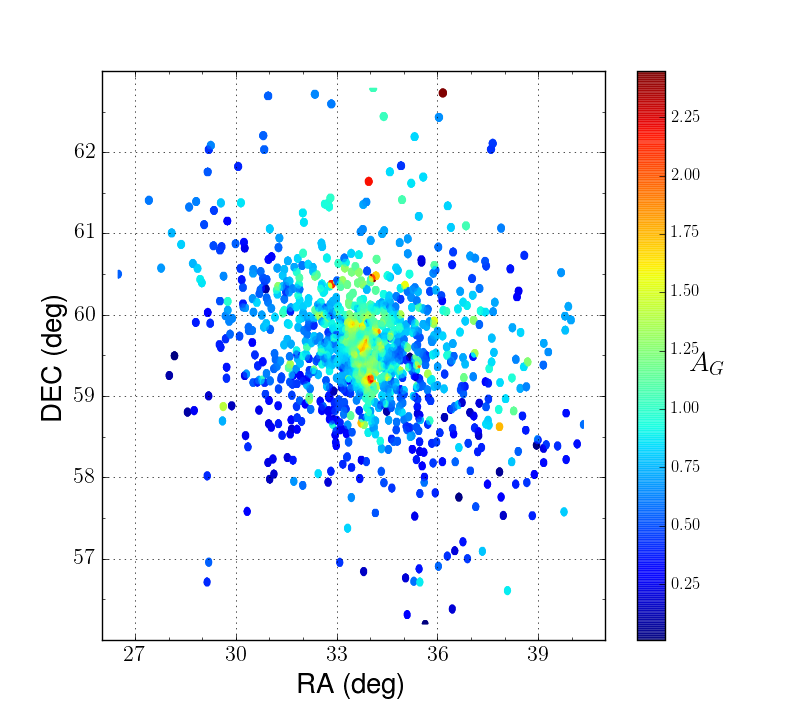
Figure 13: Interstellar extinction ($A_{G}$) towards Stock 2, as traced by the cluster members.

7 Conclusions

We have conducted this research in the framework of the SPA project with the aim of continuing to improve our knowlegde of the solar neighbourhood. This work is focused on Stock 2, a nearby and little-studied open cluster. We performed its detailed study from high-resolution spectroscopy complemented with archival photometry and $Gaia$-eDR3 data. Our sample, by far the largest to date, is composed of 46 bona-fide members, including both giants and MS stars. Among the latter, in order to study the eMSTO phenomenon, we selected the brightest stars around the TO point and many others following three different sequences to cover the spread observed in the CMDs.

We found three double spectrum binaries in our sample. For the rest of the stars we measured their radial and projected rotational velocities and derived the extinction and their atmospheric parameters. In addition, we carried out the chemical analysis for 29 stars observed with HARPS-N providing the abundances of 22 elements.

We found that half of the MS stars are fast rotators, with $v$ sin $i$¿100 km s^-1. However, the distribution of slow and fast rotators along the bMS, rMS and uMS sequences is random, which discards the rotational velocity as the cause of the observed eMSTO. Additionally, cluster members are disseminated over a wide region of the sky (up to $\approx$13^∘ $\times$ 8^∘) and differential reddening plays an important role in shaping the CMDs. We found an average reddening in the cluster field of $E(B-V)$=0.27$\pm$0.11. Its large dispersion (consistent with the $Gaia$-DR2 value, $E(G_{\textrm{BP}}-G_{\textrm{RP}})$=0.40$\pm$0.18) confirms the existence of a variable reddening across the field of Stock 2.

The reddening also makes it difficult to obtain an accurate age for the cluster. However, from the isochrone-fitting on the dereddened 2MASS CMD, which is the one less affected by the extintcion, we derived a value of 450$\pm$150 Ma. This age implies a mass at the MSTO of $\approx$2.8 M_☉. The analysis of the abundance of lithium indicates an age similar to the Hyades ($\sim 600$ Ma), although the coolest observed member could be as young as 300 Ma. Spectroscopic observations of a larger sample of members with a lower $T_{\rm eff}$ is needed to settle this point. We expect very useful data from large spectroscopic surveys that will start in the near future, such as WEAVE. The cluster RV derived from the giants is $\approx$8.0 km s^-1. Stock 2 shows a solar-like metallicity, [Fe/H]=$-$0.07$\pm$0.06, fully compatible within the errors with that expected for its Galactocentric distance.

Finally, we performed a detailed study of the cluster chemical composition by determining the abundances of C, odd-Z elements (Na, Al), $\alpha$-elements (O, Mg, Si, S, Ca, Ti), iron-peak elements (Sc, V, Cr, Mn, Co, Ni, Cu, Zn) and $s$-elements (Sr, Y, Zr, Ba). MS stars exhibit a chemical composition compatible within the errors with the giants. Only for Co and particularly for Ba and Sr diferences are significant, being the abundances of Ba and Sr clearly higher in giants. We conclude our research claiming the consistency of its chemical composition with that of the thin disc. This is supported by the values of its ratios [X/Fe] that are on the Galactic trends displayed by open clusters in the $Gaia$-ESO and APOGEE surveys. Finally, the cluster shows solar-like mean ratios for the $\alpha$ ([$\alpha$/Fe]=0.04$\pm$0.05) and the iron-peak [iron-peak/Fe]=0.03$\pm$0.03 elements while for the heaviest elements (without including the Ba and Sr abundances) exhibits a mild overabundance with respect to the Sun, [$s$/Fe]=0.17$\pm 0.04$.

Appendix A Additional material

Table 9: $Gaia$-eDR3 astrometric data and distance from the nominal cluster centre for the stars observed spectroscopically in this work.

Star	$Gaia$ ID	RA	DEC	$r$	$\mu_{\alpha*}$	$\mu_{\delta}$	$\varpi$
		(J2000)	(J2000)	($\arcmin$)	(mas yr-1)	(mas yr-1)	(mas)
b1	459178703132426240	34.48311854134	58.90486243904	31.3	14.999	$-$14.611	2.6447
b2	507116585468397056	32.54413370951	59.54252695750	40.4	16.301	$-$13.214	2.6388
b3	459194783490756864	35.39133923387	59.11965513235	51.2	15.578	$-$13.764	2.6504
b4	458990239966637952	38.27197917057	58.81579898105	142.1	14.407	$-$14.858	2.6463
b5	506840844266935936	33.97434127517	58.80312503169	28.7	15.721	$-$13.472	2.6606
b6	459222236921401728	35.07063047584	59.44654655126	41.8	15.405	$-$14.625	2.7479
b7	507255909903255552	34.84053716405	59.45844918367	35.3	15.780	$-$13.580	2.7361
b8	459218938386541952	35.16801877868	59.38902174977	44.0	15.332	$-$13.384	2.6124
r1	507146783374181632	32.13145197747	59.96836576552	64.7	14.563	$-$13.005	2.6649
r2	507365246896272896	35.06444839762	59.87623805527	54.2	15.155	$-$14.354	2.7007
r3	507252993628942720	34.05459164780	59.64717386226	24.6	15.341	$-$14.737	2.5698
r4	506860674140167040	33.76117606478	59.09963634588	10.0	15.939	$-$13.423	2.6602
r5	507320132561058816	33.33222692914	59.90338605120	40.3	15.592	$-$13.631	2.6496
r6	507292679128459648	33.44378542242	59.39912184483	12.3	16.482	$-$12.394	2.6718
r7	507314566281391872	33.15504274024	59.84529344667	39.1	15.737	$-$14.351	2.7005
r8	507310202594666368	33.29582016188	59.75533553578	32.4	16.054	$-$14.473	2.6604
u1	506860055662585216	33.90923584021	59.09157220960	11.6	16.294	$-$13.680	2.6885
u2	507226674069510656	34.15492336642	59.29460623870	12.5	16.491	$-$11.897	2.6186
u3	507222619614549120	34.08846836495	59.05499281394	16.4	15.477	$-$14.016	2.5316
u4	507300478788942336	33.82852920703	59.65770807066	23.6	15.742	$-$13.342	2.6230
u5	507296046382572544	33.43614454737	59.55110040542	19.6	15.850	$-$14.199	2.6847
u6	507327451184397568	34.11443819490	59.90860513398	40.1	15.392	$-$13.980	2.7318
g1	458067680993514880	37.96122969562	57.53016943124	168.4	15.583	$-$15.372	2.8234
g2	459199662573391104	35.31451183206	59.24791059241	48.0	15.336	$-$14.112	2.6734
g3	506910564480154624	33.36994098675	59.19599825280	12.4	16.185	$-$13.613	2.7007
g4	507507702367267584	32.79846557813	59.98091354856	51.7	15.907	$-$12.985	2.6480
g5	459118882826608640	35.40906474613	58.78418769010	58.8	15.333	$-$14.185	2.6013
g6	507214579443494144	31.49382702819	60.27836579355	91.2	16.730	$-$13.491	2.6515
g7	465132764751065984	38.41778408960	60.29074433497	153.7	14.627	$-$14.373	2.6353
g8	459112148318029056	35.44132561197	58.57339552018	66.9	16.175	$-$12.680	2.8040
g9	507240967720664576	33.81963029733	59.33494934281	4.6	17.456	$-$13.180	2.6970
g10	507520106232760320	32.66560224473	60.07874260771	58.8	16.211	$-$13.392	2.6178
to1	459223645670638080	34.96867177658	59.52776540690	40.4	15.741	$-$14.267	2.6547
to2	459214196742707328	34.89578467837	59.30823843080	35.2	15.511	$-$13.763	2.6627
to3	507833157812702464	30.38334220690	59.80312184848	107.3	16.747	$-$13.447	2.5536
to4	507254264940286848	34.59497162300	59.37600203694	26.7	15.436	$-$13.684	2.6403
to5	507289792902722560	33.50346335389	59.40154837538	11.1	16.080	$-$13.635	2.6827
to6	458031294029981056	37.33987184386	57.08988530288	173.0	15.551	$-$14.335	2.7773
to7	507289036996187392	33.67587890681	59.39470155470	8.0	16.136	$-$13.725	2.6887
to8	459047616427062656	36.71980324154	59.11633877589	91.7	15.411	$-$14.421	2.6387
to9	459349814627528832	35.90280215246	59.92113484362	76.3	15.000	$-$13.755	2.6427
to10	507270860693863552	34.39585873306	59.53594422822	25.5	15.508	$-$13.984	2.6759
to11	507242926225718656	33.88222527863	59.38491919641	8.2	15.570	$-$13.842	2.7249
to12	458972682139718400	37.53662882225	58.64313669405	123.0	14.500	$-$13.693	2.5444
to13	507233683456274176	34.36804763539	59.36682677450	19.9	15.643	$-$13.655	2.6301
to14	507299104399421696	33.71937266885	59.64359860910	22.6	15.665	$-$13.787	2.6654

Table 10: Photometry for the stars observed spectroscopically in this work.

Star	$V$	$(B-V)$	$J$	$H$	$K_{\textrm{S}}$	$G$	$(G_{\textrm{BP}}-G_{\textrm{RP}})$
b1	9.968	0.290	9.239	9.079	9.028	9.789	0.429
b2	10.067	0.287	9.278	9.191	9.158	9.976	0.484
b3	10.443	0.381	9.673	9.542	9.493	10.438	0.562
b4	10.760	0.432	9.801	9.653	9.594	10.681	0.638
b5	11.223	0.493	10.081	9.891	9.871	11.061	0.731
b6	12.459	0.684	11.132	10.795	10.705	12.308	0.927
b7	12.650	0.696	11.244	10.925	10.913	12.483	0.958
b8	13.204	0.781	11.676	11.344	11.210	13.000	1.049
r1	9.522	0.340	8.679	8.576	8.530	9.410	0.502
r2	10.019	0.355	8.992	8.919	8.820	9.825	0.602
r3	10.271	0.492	9.215	9.102	9.022	10.165	0.705
r4	10.835	0.563	9.622	9.401	9.358	10.691	0.800
r5	11.280	0.650	10.108	9.873	9.808	11.172	0.835
r6	11.793	0.675	10.414	10.127	10.045	11.602	0.937
r7	12.610	0.855	11.124	10.739	10.657	12.405	1.075
r8	13.075	0.891	11.481	11.079	11.035	12.854	1.122
u1	9.559	0.564	8.359	8.277	8.158	9.379	0.770
u2	10.085	0.569	8.752	8.553	8.460	9.849	0.844
u3	10.725	0.680	9.315	9.119	9.017	10.529	0.952
u4	11.570	0.867	9.889	9.689	9.573	11.334	1.132
u5	12.078	0.923	10.277	10.000	9.855	11.784	1.198
u6	13.111	1.000	11.074	10.776	10.652	12.769	1.334
g1	7.132	1.348	4.764	3.920	3.730	6.689	1.476
g2	7.492	1.233	5.167	4.597	4.449	7.006	1.454
g3	7.633	1.189	5.394	4.889	4.718	7.199	1.433
g4	8.222	1.234	5.915	5.367	5.213	7.782	1.466
g5	8.201	1.085	6.153	5.657	5.520	7.819	1.306
g6	8.402	1.410	5.878	5.286	5.148	7.879	1.582
g7	8.401	1.192	6.117	5.593	5.438	7.960	1.441
g8	8.359	1.003	6.410	5.916	5.813	7.999	1.252
g9	8.892	1.342	6.195	5.632	5.450	8.309	1.701
g10	8.975	1.144	6.639	6.131	5.986	8.497	1.458
to1	8.220	0.215	7.606	7.669	7.585	8.134	0.317
to2	8.291	0.297	7.517	7.476	7.411	8.194	0.447
to3	8.324	0.236	7.662	7.650	7.571	8.241	0.369
to4	8.527	0.342	7.666	7.568	7.534	8.399	0.501
to5	8.585	0.407	7.655	7.557	7.518	8.475	0.580
to6	8.632	0.182	8.171	8.143	8.094	8.551	0.248
to7	8.704	0.445	7.683	7.613	7.552	8.575	0.619
to8	8.666	0.222	8.042	8.031	7.991	8.583	0.340
to9	8.734	0.437	7.727	7.591	7.509	8.585	0.625
to10	8.708	0.357	7.859	7.783	7.729	8.605	0.514
to11	8.779	0.429	7.747	7.701	7.613	8.633	0.620
to12	8.744	0.219	8.121	8.125	8.045	8.656	0.340
to13	8.812	0.347	7.886	7.798	7.750	8.679	0.537
to14	9.041	0.477	7.906	7.815	7.698	8.883	0.719

Table 11: Chemical abundances, expressed as $A(X)$=log[$n(X)/n(H)$]+12, for MS stars in Stock 2.

X	b1	b2	b4	b5	b6	b7	b8	r3
C	8.66 $\pm$ 0.09	8.67 $\pm$ 0.18	8.47 $\pm$ 0.08	8.65 $\pm$ 0.17	$\dots$	8.32 $\pm$ 0.11	$\dots$	8.35 $\pm$ 0.15
O	8.57 $\pm$ 0.13	8.53 $\pm$ 0.11	8.41 $\pm$ 0.16	$\dots$	$\dots$	$\dots$	$\dots$	8.29 $\pm$ 0.15
Na	$\dots$	$\dots$	6.42 $\pm$ 0.15	6.44 $\pm$ 0.15	6.29 $\pm$ 0.15	6.23 $\pm$ 0.09	6.26 $\pm$ 0.04	6.15 $\pm$ 0.13
Mg	7.54 $\pm$ 0.07	7.55 $\pm$ 0.15	7.52 $\pm$ 0.13	7.60 $\pm$ 0.15	7.33 $\pm$ 0.05	7.40 $\pm$ 0.09	7.47 $\pm$ 0.13	7.53 $\pm$ 0.12
Al	$\dots$	$\dots$	$\dots$	$\dots$	$\dots$	6.10 $\pm$ 0.15	6.30 $\pm$ 0.10	$\dots$
Si	7.56 $\pm$ 0.19	7.66 $\pm$ 0.12	7.57 $\pm$ 0.10	$\dots$	7.46 $\pm$ 0.15	7.44 $\pm$ 0.09	7.58 $\pm$ 0.05	7.59 $\pm$ 0.11
S	7.29 $\pm$ 0.15	$\dots$	7.23 $\pm$ 0.15	$\dots$	$\dots$	7.41 $\pm$ 0.15	$\dots$	7.45 $\pm$ 0.15
Ca	6.33 $\pm$ 0.16	6.12 $\pm$ 0.14	6.19 $\pm$ 0.11	6.37 $\pm$ 0.10	6.48 $\pm$ 0.12	6.31 $\pm$ 0.15	6.35 $\pm$ 0.12	$\dots$
Sc	3.38 $\pm$ 0.10	3.19 $\pm$ 0.15	3.24 $\pm$ 0.15	$\dots$	3.01 $\pm$ 0.15	2.99 $\pm$ 0.13	3.18 $\pm$ 0.07	3.19 $\pm$ 0.15
Ti	4.91 $\pm$ 0.17	4.85 $\pm$ 0.19	5.00 $\pm$ 0.17	$\dots$	4.99 $\pm$ 0.15	4.76 $\pm$ 0.06	4.89 $\pm$ 0.11	4.62 $\pm$ 0.10
V	4.21 $\pm$ 0.15	4.09 $\pm$ 0.14	4.13 $\pm$ 0.15	$\dots$	3.96 $\pm$ 0.15	3.81 $\pm$ 0.19	4.08 $\pm$ 0.18	4.41 $\pm$ 0.15
Cr	5.54 $\pm$ 0.11	5.73 $\pm$ 0.14	5.56 $\pm$ 0.12	$\dots$	5.53 $\pm$ 0.14	5.50 $\pm$ 0.11	5.68 $\pm$ 0.15	5.59 $\pm$ 0.14
Mn	5.41 $\pm$ 0.15	5.43 $\pm$ 0.14	5.35 $\pm$ 0.15	5.35 $\pm$ 0.15	5.20 $\pm$ 0.16	5.17 $\pm$ 0.15	5.42 $\pm$ 0.20	5.35 $\pm$ 0.15
Fe	7.49 $\pm$ 0.19	7.61 $\pm$ 0.12	7.02 $\pm$ 0.15	7.40 $\pm$ 0.10	7.39 $\pm$ 0.15	7.31 $\pm$ 0.10	7.25 $\pm$ 0.12	7.06 $\pm$ 0.18
Co	4.88 $\pm$ 0.15	$\dots$	4.88 $\pm$ 0.15	4.88 $\pm$ 0.10	5.00 $\pm$ 0.15	4.71 $\pm$ 0.15	4.89 $\pm$ 0.18	5.07 $\pm$ 0.09
Ni	6.28 $\pm$ 0.14	6.50 $\pm$ 0.09	6.07 $\pm$ 0.17	$\dots$	6.12 $\pm$ 0.14	6.02 $\pm$ 0.17	6.07 $\pm$ 0.11	6.25 $\pm$ 0.20
Cu	$\dots$	$\dots$	$\dots$	$\dots$	$\dots$	4.07 $\pm$ 0.11	4.00 $\pm$ 0.16	$\dots$
Zn	$\dots$	$\dots$	4.31 $\pm$ 0.15	$\dots$	4.32 $\pm$ 0.15	4.32 $\pm$ 0.06	$\dots$	4.58 $\pm$ 0.15
Sr	2.86 $\pm$ 0.15	3.05 $\pm$ 0.13	3.01 $\pm$ 0.15	$\dots$	2.90 $\pm$ 0.15	3.02 $\pm$ 0.13	2.90 $\pm$ 0.10	2.90 $\pm$ 0.04
Y	2.26 $\pm$ 0.19	2.57 $\pm$ 0.19	2.30 $\pm$ 0.11	$\dots$	2.14 $\pm$ 0.08	2.21 $\pm$ 0.19	2 .19 $\pm$ 0.09	2.25 $\pm$ 0.11
Zr	$\dots$	$\dots$	2.56 $\pm$ 0.15	$\dots$	2.56 $\pm$ 0.15	2.64 $\pm$ 0.11	2.76 $\pm$ 0.15	2.40 $\pm$ 0.16
Ba	1.84 $\pm$ 0.15	2.64 $\pm$ 0.12	1.63 $\pm$ 0.19	$\dots$	1.97 $\pm$ 0.15	2.03 $\pm$ 0.19	2.09 $\pm$ 0.15	1.95 $\pm$ 0.11
X	r5	r6	r7	r8	u3	u4	u5	u6
C	8.66 $\pm$ 0.11	8.50 $\pm$ 0.13	8.61 $\pm$ 0.15	8.27 $\pm$ 0.08	8.41 $\pm$ 0.15	8.42 $\pm$ 0.11	8.07 $\pm$ 0.15	8.62 $\pm$ 0.17
O	8.45 $\pm$ 0.08	8.79 $\pm$ 0.18	$\dots$	$\dots$	8.65 $\pm$ 0.04	8.78 $\pm$ 0.11	$\dots$	$\dots$
Na	$\dots$	6.44 $\pm$ 0.15	6.11 $\pm$ 0.14	6.13 $\pm$ 0.08	6.21 $\pm$ 0.14	$\dots$	6.29 $\pm$ 0.09	6.20 $\pm$ 0.17
Mg	7.44 $\pm$ 0.13	7.40 $\pm$ 0.10	7.40 $\pm$ 0.13	7.43 $\pm$ 0.11	7.32 $\pm$ 0.11	7.59 $\pm$ 0.06	7.56 $\pm$ 0.15	7.42 $\pm$ 0.10
Al	$\dots$	6.45 $\pm$ 0.10	$\dots$	6.50 $\pm$ 0.10	$\dots$	$\dots$	$\dots$	6.30 $\pm$ 0.15
Si	7.58 $\pm$ 0.18	7.48 $\pm$ 0.12	7.43 $\pm$ 0.15	7.51 $\pm$ 0.09	7.33 $\pm$ 0.12	7.61 $\pm$ 0.15	7.61 $\pm$ 0.19	7.45 $\pm$ 0.17
S	$\dots$	7.38 $\pm$ 0.12	7.33 $\pm$ 0.19	7.19 $\pm$ 0.20	7.35 $\pm$ 0.08	7.29 $\pm$ 0.15	$\dots$	7.20 $\pm$ 0.14
Ca	6.35 $\pm$ 0.19	6.20 $\pm$ 0.09	6.33 $\pm$ 0.11	6.42 $\pm$ 0.10	6.12 $\pm$ 0.17	6.27 $\pm$ 0.12	6.37 $\pm$ 0.18	6.31 $\pm$ 0.11
Sc	3.13 $\pm$ 0.10	2.93 $\pm$ 0.10	3.23 $\pm$ 0.17	3.06 $\pm$ 0.12	3.19 $\pm$ 0.09	3.07 $\pm$ 0.11	3.13 $\pm$ 0.10	3.18 $\pm$ 0.15
Ti	4.75 $\pm$ 0.05	4.82 $\pm$ 0.14	4.73 $\pm$ 0.15	4.91 $\pm$ 0.12	4.56 $\pm$ 0.14	4.73 $\pm$ 0.10	4.99 $\pm$ 0.13	4.61 $\pm$ 0.14
V	4.04 $\pm$ 0.14	3.98 $\pm$ 0.16	4.23 $\pm$ 0.11	4.01 $\pm$ 0.16	4.05 $\pm$ 0.08	4.17 $\pm$ 0.19	4.22 $\pm$ 0.15	4.06 $\pm$ 0.16
Cr	5.52 $\pm$ 0.16	5.48 $\pm$ 0.11	5.34 $\pm$ 0.12	5.61 $\pm$ 0.09	5.29 $\pm$ 0.11	5.64 $\pm$ 0.09	5.63 $\pm$ 0.08	5.28 $\pm$ 0.11
Mn	4.97 $\pm$ 0.13	5.13 $\pm$ 0.14	5.27 $\pm$ 0.11	5.39 $\pm$ 0.17	5.05 $\pm$ 0.13	5.10 $\pm$ 0.15	5.48 $\pm$ 0.14	5.22 $\pm$ 0.15
Fe	7.20 $\pm$ 0.10	7.15 $\pm$ 0.14	7.14 $\pm$ 0.12	7.43 $\pm$ 0.08	7.10 $\pm$ 0.15	7.37 $\pm$ 0.16	7.33 $\pm$ 0.13	7.18 $\pm$ 0.15
Co	5.23 $\pm$ 0.15	5.10 $\pm$ 0.20	5.16 $\pm$ 0.09	4.89 $\pm$ 0.18	5.00 $\pm$ 0.20	5.03 $\pm$ 0.15	5.32 $\pm$ 0.11	4.91 $\pm$ 0.08
Ni	6.08 $\pm$ 0.15	5.90 $\pm$ 0.11	5.91 $\pm$ 0.17	6.12 $\pm$ 0.18	6.00 $\pm$ 0.11	6.25 $\pm$ 0.17	6.21 $\pm$ 0.08	5.97 $\pm$ 0.17
Cu	4.17 $\pm$ 0.15	4.30 $\pm$ 0.15	4.11 $\pm$ 0.15	4.08 $\pm$ 0.04	$\dots$	$\dots$	$\dots$	4.24 $\pm$ 0.15
Zn	$\dots$	4.22 $\pm$ 0.11	4.15 $\pm$ 0.13	4.43 $\pm$ 0.10	$\dots$	$\dots$	$\dots$	4.35 $\pm$ 0.15
Sr	$\dots$	2.93 $\pm$ 0.10	$\dots$	3.00 $\pm$ 0.04	2.89 $\pm$ 0.04	2.87 $\pm$ 0.15	$\dots$	3.03 $\pm$ 0.15
Y	$\dots$	2.29 $\pm$ 0.11	2.50 $\pm$ 0.05	2.28 $\pm$ 0.19	2.48 $\pm$ 0.04	2.24 $\pm$ 0.19	2.20 $\pm$ 0.15	2.00 $\pm$ 0.15
Zr	2.56 $\pm$ 0.14	2.66 $\pm$ 0.14	2.62 $\pm$ 0.17	2.70 $\pm$ 0.19	2.82 $\pm$ 0.08	$\dots$	$\dots$	2.57 $\pm$ 0.14
Ba	1.61 $\pm$ 0.16	1.89 $\pm$ 0.14	1.91 $\pm$ 0.08	2.03 $\pm$ 0.08	1.39 $\pm$ 0.14	2.06 $\pm$ 0.04	2.14 $\pm$ 0.18	2.05 $\pm$ 0.13

Table 12: Chemical abundances, expressed as $A(X)$=log[$n(X)/n(H)$]+12, for giants in Stock 2.

X	g1	g2	g3	g4	g5	g6	g7	g8	g9	g10
Na	6.35 $\pm$ 0.08	6.38 $\pm$ 0.15	6.56 $\pm$ 0.13	6.49 $\pm$ 0.13	6.39 $\pm$ 0.10	6.56 $\pm$ 0.15	6.50 $\pm$ 0.10	6.31 $\pm$ 0.10	6.46 $\pm$ 0.13	6.35 $\pm$ 0.06
Mg	7.59 $\pm$ 0.12	7.52 $\pm$ 0.13	7.58 $\pm$ 0.09	7.55 $\pm$ 0.03	7.51 $\pm$ 0.12	7.54 $\pm$ 0.06	7.63 $\pm$ 0.15	7.47 $\pm$ 0.15	7.71 $\pm$ 0.18	7.52 $\pm$ 0.16
Al	6.37 $\pm$ 0.08	6.46 $\pm$ 0.09	6.41 $\pm$ 0.02	6.48 $\pm$ 0.17	6.56 $\pm$ 0.13	6.41 $\pm$ 0.12	6.48 $\pm$ 0.14	6.56 $\pm$ 0.13	6.68 $\pm$ 0.10	6.50 $\pm$ 0.10
Si	7.63 $\pm$ 0.09	7.58 $\pm$ 0.12	7.60 $\pm$ 0.12	7.57 $\pm$ 0.13	7.54 $\pm$ 0.09	7.58 $\pm$ 0.11	7.57 $\pm$ 0.12	7.48 $\pm$ 0.12	7.57 $\pm$ 0.11	7.54 $\pm$ 0.13
S	$\dots$	$\dots$	7.49 $\pm$ 0.13	7.41 $\pm$ 0.18	7.54 $\pm$ 0.15	7.47 $\pm$ 0.15	7.47 $\pm$ 0.15	7.47 $\pm$ 0.16	7.47 $\pm$ 0.26	7.44 $\pm$ 0.12
Ca	6.24 $\pm$ 0.15	6.20 $\pm$ 0.15	6.28 $\pm$ 0.15	6.30 $\pm$ 0.15	6.30 $\pm$ 0.14	6.25 $\pm$ 0.10	6.21 $\pm$ 0.12	6.22 $\pm$ 0.15	6.20 $\pm$ 0.15	6.11 $\pm$ 0.15
Sc	3.09 $\pm$ 0.07	3.18 $\pm$ 0.14	3.21 $\pm$ 0.12	3.24 $\pm$ 0.12	3.16 $\pm$ 0.10	3.16 $\pm$ 0.13	3.23 $\pm$ 0.12	3.23 $\pm$ 0.14	3.23 $\pm$ 0.14	3.16 $\pm$ 0.13
Ti	4.78 $\pm$ 0.15	4.77 $\pm$ 0.15	4.94 $\pm$ 0.15	4.90 $\pm$ 0.10	4.86 $\pm$ 0.13	4.94 $\pm$ 0.15	4.87 $\pm$ 0.11	4.79 $\pm$ 0.15	4.84 $\pm$ 0.14	4.79 $\pm$ 0.15
V	3.90 $\pm$ 0.16	3.93 $\pm$ 0.09	3.97 $\pm$ 0.15	3.94 $\pm$ 0.15	3.90 $\pm$ 0.13	3.90 $\pm$ 0.15	3.97 $\pm$ 0.15	3.88 $\pm$ 0.12	3.96 $\pm$ 0.08	3.88 $\pm$ 0.12
Cr	5.64 $\pm$ 0.12	5.65 $\pm$ 0.13	5.70 $\pm$ 0.12	5.73 $\pm$ 0.12	5.62 $\pm$ 0.07	5.72 $\pm$ 0.12	5.73 $\pm$ 0.12	5.63 $\pm$ 0.05	5.68 $\pm$ 0.12	5.65 $\pm$ 0.14
Mn	5.29 $\pm$ 0.10	5.30 $\pm$ 0.12	5.34 $\pm$ 0.11	5.29 $\pm$ 0.10	5.34 $\pm$ 0.08	5.31 $\pm$ 0.09	5.28 $\pm$ 0.11	5.28 $\pm$ 0.13	5.27 $\pm$ 0.11	5.28 $\pm$ 0.11
Fe	7.30 $\pm$ 0.19	7.30 $\pm$ 0.13	7.45 $\pm$ 0.09	7.35 $\pm$ 0.14	7.29 $\pm$ 0.11	7.40 $\pm$ 0.13	7.31 $\pm$ 0.12	7.34 $\pm$ 0.12	7.28 $\pm$ 0.15	7.30 $\pm$ 0.14
Co	4.83 $\pm$ 0.13	4.87 $\pm$ 0.07	4.81 $\pm$ 0.10	4.83 $\pm$ 0.14	4.87 $\pm$ 0.13	4.82 $\pm$ 0.13	4.82 $\pm$ 0.11	4.85 $\pm$ 0.13	4.93 $\pm$ 0.13	4.78 $\pm$ 0.12
Ni	6.04 $\pm$ 0.11	6.00 $\pm$ 0.15	6.17 $\pm$ 0.13	6.17 $\pm$ 0.14	6.09 $\pm$ 0.14	6.19 $\pm$ 0.14	6.20 $\pm$ 0.13	6.03 $\pm$ 0.13	6.09 $\pm$ 0.15	6.00 $\pm$ 0.09
Cu	3.88 $\pm$ 0.15	3.96 $\pm$ 0.14	4.11 $\pm$ 0.15	3.99 $\pm$ 0.15	3.96 $\pm$ 0.11	3.96 $\pm$ 0.15	3.99 $\pm$ 0.12	3.90 $\pm$ 0.11	3.93 $\pm$ 0.15	3.87 $\pm$ 0.15
Zn	4.53 $\pm$ 0.15	4.25 $\pm$ 0.09	4.42 $\pm$ 0.12	4.35 $\pm$ 0.08	4.32 $\pm$ 0.10	4.47 $\pm$ 0.10	4.55 $\pm$ 0.12	4.49 $\pm$ 0.09	4.39 $\pm$ 0.10	4.33 $\pm$ 0.15
Sr	3.03 $\pm$ 0.20	3.31 $\pm$ 0.13	3.53 $\pm$ 0.13	3.43 $\pm$ 0.10	3.51 $\pm$ 0.10	3.31 $\pm$ 0.14	3.36 $\pm$ 0.14	3.46 $\pm$ 0.11	3.30 $\pm$ 0.15	3.43 $\pm$ 0.10
Y	2.37 $\pm$ 0.13	2.40 $\pm$ 0.12	2.36 $\pm$ 0.13	2.30 $\pm$ 0.13	2.36 $\pm$ 0.12	2.23 $\pm$ 0.13	2.13 $\pm$ 0.15	2.34 $\pm$ 0.14	2.21 $\pm$ 0.13	2.39 $\pm$ 0.18
Zr	2.59 $\pm$ 0.15	2.71 $\pm$ 0.05	2.62 $\pm$ 0.08	2.64 $\pm$ 0.12	2.66 $\pm$ 0.12	2.59 $\pm$ 0.05	2.64 $\pm$ 0.14	2.62 $\pm$ 0.14	2.66 $\pm$ 0.12	2.64 $\pm$ 0.14
Ba	2.47 $\pm$ 0.18	2.42 $\pm$ 0.05	2.34 $\pm$ 0.06	2.30 $\pm$ 0.04	2.25 $\pm$ 0.09	2.47 $\pm$ 0.14	2.47 $\pm$ 0.14	2.47 $\pm$ 0.10	2.40 $\pm$ 0.18	2.42 $\pm$ 0.12

References

- Allard (2014) Allard, F. 2014, in Exploring the Formation and Evolution of Planetary Systems, ed. M. Booth, B. C. Matthews, & J. R. Graham, Vol. 299, 271–272
- Alonso-Santiago et al. (2018) Alonso-Santiago, J., Marco, A., Negueruela, I., et al. 2018, A&A, 616, A124
- Alonso-Santiago et al. (2020) Alonso-Santiago, J., Negueruela, I., Marco, A., Tabernero, H. M., & Castro, N. 2020, A&A, 644, A136
- Alonso-Santiago et al. (2017) Alonso-Santiago, J., Negueruela, I., Marco, A., et al. 2017, MNRAS, 469, 1330
- Alonso-Santiago et al. (2019) Alonso-Santiago, J., Negueruela, I., Marco, A., et al. 2019, A&A, 631, A124
- Baratella et al. (2020) Baratella, M., D’Orazi, V., Carraro, G., et al. 2020, A&A, 634, A34
- Bastian et al. (2017) Bastian, N., Cabrera-Ziri, I., Niederhofer, F., et al. 2017, MNRAS, 465, 4795
- Bressan et al. (2012) Bressan, A., Marigo, P., Girardi, L., et al. 2012, MNRAS, 427, 127
- Cantat-Gaudin et al. (2018) Cantat-Gaudin, T., Jordi, C., Vallenari, A., et al. 2018, A&A, 618, A93
- Casali et al. (2020) Casali, G., Magrini, L., Frasca, A., et al. 2020, A&A, 643, A12
- Catanzaro et al. (2011) Catanzaro, G., Ripepi, V., Bernabei, S., et al. 2011, MNRAS, 411, 1167
- Catanzaro et al. (2013) Catanzaro, G., Ripepi, V., & Bruntt, H. 2013, MNRAS, 431, 3258
- Cordoni et al. (2018) Cordoni, G., Milone, A. P., Marino, A. F., et al. 2018, ApJ, 869, 139
- Correnti et al. (2017) Correnti, M., Goudfrooij, P., Bellini, A., Kalirai, J. S., & Puzia, T. H. 2017, MNRAS, 467, 3628
- Cosentino et al. (2014) Cosentino, R., Lovis, C., Pepe, F., et al. 2014, in Society of Photo-Optical Instrumentation Engineers (SPIE) Conference Series, Vol. 9147, Ground-based and Airborne Instrumentation for Astronomy V, ed. S. K. Ramsay, I. S. McLean, & H. Takami, 91478C
- Dalton et al. (2020) Dalton, G., Trager, S., Abrams, D. C., et al. 2020, in Society of Photo-Optical Instrumentation Engineers (SPIE) Conference Series, Vol. 11447, Society of Photo-Optical Instrumentation Engineers (SPIE) Conference Series, 1144714
- D’Antona et al. (2015) D’Antona, F., Di Criscienzo, M., Decressin, T., et al. 2015, MNRAS, 453, 2637
- D’Antona et al. (2017) D’Antona, F., Milone, A. P., Tailo, M., et al. 2017, Nature Astronomy, 1, 0186
- Donor et al. (2020) Donor, J., Frinchaboy, P. M., Cunha, K., et al. 2020, AJ, 159, 199
- D’Orazi et al. (2020) D’Orazi, V., Oliva, E., Bragaglia, A., et al. 2020, A&A, 633, A38
- Dupree et al. (2017) Dupree, A. K., Dotter, A., Johnson, C. I., et al. 2017, ApJ, 846, L1
- Frasca et al. (2019) Frasca, A., Alonso-Santiago, J., Catanzaro, G., et al. 2019, A&A, 632, A16
- Frasca et al. (2015) Frasca, A., Biazzo, K., Lanzafame, A. C., et al. 2015, A&A, 575, A4
- Frasca et al. (2018) Frasca, A., Guillout, P., Klutsch, A., et al. 2018, A&A, 612, A96
- Frasca et al. (2006) Frasca, A., Guillout, P., Marilli, E., et al. 2006, A&A, 454, 301
- Gaia Collaboration et al. (2021) Gaia Collaboration, Brown, A. G. A., Vallenari, A., et al. 2021, A&A, 649, A1
- Gossage et al. (2019) Gossage, S., Conroy, C., Dotter, A., et al. 2019, ApJ, 887, 199
- Goudfrooij et al. (2017) Goudfrooij, P., Girardi, L., & Correnti, M. 2017, ApJ, 846, 22
- Gratton et al. (2019) Gratton, R., Bragaglia, A., Carretta, E., et al. 2019, A&A Rev., 27, 8
- Grevesse et al. (2007) Grevesse, N., Asplund, M., & Sauval, A. J. 2007, Space Sci. Rev., 130, 105
- Henden et al. (2016) Henden, A. A., Templeton, M., Terrell, D., et al. 2016, VizieR Online Data Catalog, II/336
- Jeffries (2014) Jeffries, R. D. 2014, in EAS Publications Series, Vol. 65, EAS Publications Series, 289–325
- Johnston et al. (2019) Johnston, C., Aerts, C., Pedersen, M. G., & Bastian, N. 2019, A&A, 632, A74
- Kharchenko & Roeser (2009) Kharchenko, N. V. & Roeser, S. 2009, VizieR Online Data Catalog, I/280B
- Krumholz et al. (2019) Krumholz, M. R., McKee, C. F., & Bland-Hawthorn, J. 2019, ARA&A, 57, 227
- Krzeminski & Serkowski (1967) Krzeminski, W. & Serkowski, K. 1967, ApJ, 147, 988
- Kurucz (1993a) Kurucz, R. 1993a, ATLAS9 Stellar Atmosphere Programs and 2 km/s grid. Kurucz CD-ROM No. 13. Cambridge, 13
- Kurucz (1993b) Kurucz, R. L. 1993b, in Astronomical Society of the Pacific Conference Series, Vol. 44, IAU Colloq. 138: Peculiar versus Normal Phenomena in A-type and Related Stars, ed. M. M. Dworetsky, F. Castelli, & R. Faraggiana, 87
- Kurucz & Avrett (1981) Kurucz, R. L. & Avrett, E. H. 1981, SAO Special Report, 391
- Lallement et al. (2019) Lallement, R., Babusiaux, C., Vergely, J. L., et al. 2019, A&A, 625, A135
- Leone et al. (2016) Leone, F., Avila, G., Bellassai, G., et al. 2016, AJ, 151, 116
- Li et al. (2017) Li, C., de Grijs, R., Deng, L., & Milone, A. P. 2017, ApJ, 844, 119
- Li et al. (2019) Li, C., Sun, W., de Grijs, R., et al. 2019, ApJ, 876, 65
- Lind et al. (2009) Lind, K., Asplund, M., & Barklem, P. S. 2009, A&A, 503, 541
- Lindegren et al. (2021) Lindegren, L., Bastian, U., Biermann, M., et al. 2021, A&A, 649, A4
- Mackey & Broby Nielsen (2007) Mackey, A. D. & Broby Nielsen, P. 2007, MNRAS, 379, 151
- Magrini et al. (2021) Magrini, L., Lagarde, N., Charbonnel, C., et al. 2021, A&A, 651, A84
- Magrini et al. (2017) Magrini, L., Randich, S., Kordopatis, G., et al. 2017, A&A, 603, A2
- Magrini et al. (2018) Magrini, L., Spina, L., Randich, S., et al. 2018, A&A, 617, A106
- Marino et al. (2018a) Marino, A. F., Milone, A. P., Casagrande, L., et al. 2018a, ApJ, 863, L33
- Marino et al. (2018b) Marino, A. F., Przybilla, N., Milone, A. P., et al. 2018b, AJ, 156, 116
- Mermilliod et al. (2008) Mermilliod, J. C., Mayor, M., & Udry, S. 2008, A&A, 485, 303
- Milone et al. (2009) Milone, A. P., Bedin, L. R., Piotto, G., & Anderson, J. 2009, A&A, 497, 755
- Milone et al. (2016) Milone, A. P., Marino, A. F., D’Antona, F., et al. 2016, MNRAS, 458, 4368
- Milone et al. (2018) Milone, A. P., Marino, A. F., Di Criscienzo, M., et al. 2018, MNRAS, 477, 2640
- Niederhofer et al. (2015) Niederhofer, F., Georgy, C., Bastian, N., & Ekström, S. 2015, MNRAS, 453, 2070
- Origlia et al. (2019) Origlia, L., Dalessandro, E., Sanna, N., et al. 2019, A&A, 629, A117
- Piatti & Bonatto (2019) Piatti, A. E. & Bonatto, C. 2019, MNRAS, 490, 2414
- Reddy & Lambert (2019) Reddy, A. B. S. & Lambert, D. L. 2019, MNRAS, 485, 3623
- Robichon et al. (1999) Robichon, N., Arenou, F., Mermilliod, J.-C., & Turon, C. 1999, A&A, 345, 471
- Sciortino et al. (2000) Sciortino, S., Micela, G., Favata, F., Spagna, A., & Lattanzi, M. G. 2000, A&A, 357, 460
- Sestito & Randich (2005) Sestito, P. & Randich, S. 2005, A&A, 442, 615
- Skrutskie et al. (2006) Skrutskie, M. F., Cutri, R. M., Stiening, R., et al. 2006, AJ, 131, 1163
- Smiljanic et al. (2014) Smiljanic, R., Korn, A. J., Bergemann, M., et al. 2014, A&A, 570, A122
- Spagna et al. (2009) Spagna, A., Cossu, F., Lattanzi, M. G., & Massone, G. 2009, Mem. Soc. Astron. Italiana, 80, 129
- Spanò et al. (2006) Spanò, P., Leone, F., Bruno, P., et al. 2006, Memorie della Societa Astronomica Italiana Supplementi, 9, 481
- Stock (1956) Stock, J. 1956, ApJ, 123, 258
- Straižys & Lazauskaitė (2009) Straižys, V. & Lazauskaitė, R. 2009, Baltic Astronomy, 18, 19
- Sun et al. (2019) Sun, W., de Grijs, R., Deng, L., & Albrow, M. D. 2019, ApJ, 876, 113
- Ye et al. (2021) Ye, X., Zhao, J., Liu, J., et al. 2021, AJ, 161, 8
- Zhang et al. (2021) Zhang, R., Lucatello, S., Bragaglia, A., et al. 2021, arXiv e-prints, arXiv:2106.08014